Classification of amyloid status using machine learning ...adni.loni.usc.edu/adni-publications/Cattell_2016_neuroimageClin.pdf · Brain amyloid burden may be quantitatively assessed

NeuroImage: Clinical 12 (2016) 990–1003

Contents lists available at ScienceDirect

NeuroImage: Clinical

j ourna l homepage: www.e lsev ie r .com/ locate /yn ic l

Classification of amyloid status using machine learning with histogramsof oriented 3D gradients

Liam Cattella,⁎, Günther Platschb, Richie Pfeifferc, Jérôme Declerckb, Julia A. Schnabeld, Chloe Huttonb,for the Alzheimer's Disease Neuroimaging Initiative1:aInstitute of Biomedical Engineering, Department of Engineering Science, University of Oxford, UKbSiemens Molecular Imaging, Oxford, UKcPiramal Imaging, Berlin, GermanydDivision of Imaging Sciences and Biomedical Engineering, King's College London, UK

⁎ Corresponding author.E-mail address: [email protected] (L. Cattell).

1 Data used in preparation of this article were obtaineNeuroimaging Initiative (ADNI) database (adni.loni.usc.ewithin the ADNI contributed to the design and implemendata but did not participate in analysis or writing of thADNI investigators can be found at: http://adni.loni.usc.eto_apply/ADNI_Acknowledgemen_List.pdf.

http://dx.doi.org/10.1016/j.nicl.2016.05.0042213-1582/© 2016 The Authors. Published by Elsevier Inc

a b s t r a c t

Article history:Received 4 November 2015Received in revised form 28 April 2016Accepted 3 May 2016Available online 10 May 2016

Brain amyloid burden may be quantitatively assessed from positron emission tomography imaging usingstandardised uptake value ratios. Using these ratios as an adjunct to visual image assessment has been shownto improve inter-reader reliability, however, the amyloid positivity threshold is dependent on the tracer and spe-cific image regions used to calculate the uptake ratio. To address this problem, we propose a machine learningapproach to amyloid status classification, which is independent of tracer and does not require a specific set of re-gions of interest. Our method extracts feature vectors from amyloid images, which are based on histograms oforiented three-dimensional gradients. We optimised our method on 133 18F-florbetapir brain volumes, and ap-plied it to a separate test set of 131 volumes. Using the same parameter settings, we then applied our method to209 11C-PiB images and 128 18F-florbetaben images. We compared our method to classification results achievedusing two othermethods: standardised uptake value ratios and amachine learningmethod based on voxel inten-sities. Our method resulted in the largest mean distances between the subjects and the classification boundary,suggesting that it is less likely to make low-confidence classification decisions. Moreover, our method obtainedthe highest classification accuracy for all three tracers, and consistently achieved above 96% accuracy.

© 2016 The Authors. Published by Elsevier Inc. This is an open access article under the CC BY license(http://creativecommons.org/licenses/by/4.0/).

Keywords:AmyloidPositron emission tomographyFlorbetapirFlorbetabenPittsburgh compound BClassification

1. Introduction

Positron emission tomography (PET) is increasingly used to assessthe burden of fibrillar β-amyloid in patients with suspected Alzheimer'sdisease (AD). Elevated levels of β-amyloid, in the form of plaques, are apathological biomarker of the disease. The first tracer to specificallyimage these plaques in neuronal tissue was 11C-Pittsburgh Com-pound-B (11C-PiB) (Klunk et al., 2004). Due to the short half-life of car-bon-11 (20 min), the compound needs to be prepared on-site and usedimmediately. This requires a cyclotron in the hospital, which is uncom-mon, and hencemakes 11C-PiB impractical for routine clinical use. Morerecently, several other amyloid tracers have been developed using thefluorine-18 isotope, which has a longer half-life of 110 min and allows

d from the Alzheimer's Diseasedu). As such, the investigatorstation of ADNI and/or providedis report. A complete listing ofdu/wp-content/uploads/how_

. This is an open access article under

regional distribution. Three of these have recently been approved bytheUS Food andDrug Administration (FDA) for use in clinical diagnosis:18F-florbetapir, 18F-flutemetamol, and 18F-florbetaben (FDA, 2012,2013; Piramal, 2014).

Prior to regulatory approval, the FDA and EuropeanMedicines Asso-ciation (EMA) gave much attention to consistency of F-18 amyloidimage interpretation between readers (EMA Committee for MedicinalProducts for Human Use, 2013; FDA Peripheral and Central NervousSystem Drugs Advisory Committee, 2010). Consequently, thoroughreader training programmes have been developed for visual interpreta-tion. However, as reported by Frey (2015), a lack of concordance be-tween independent readers suggests the need for additional analyticalapproaches to clinical reading and reporting.

Brain amyloid burden can be evaluated quantitatively by calculatingthe ratio of tracer uptake in a set of target brain regions to non-specifictracer uptake in a reference region (Barthel et al., 2011; Fleisher et al.,2011; Jack et al., 2008; Jagust et al., 2009; Joshi et al., 2012;Villemagne et al., 2011). This ratio is known as the standardised uptakevalue ratio (SUVR). Typically, the individual SUVRs for each target re-gion are averaged to form the mean, or composite, SUVR (Rowe et al.,2008). It has been shown that incorporating this ratio as an adjunct to

the CC BY license (http://creativecommons.org/licenses/by/4.0/).

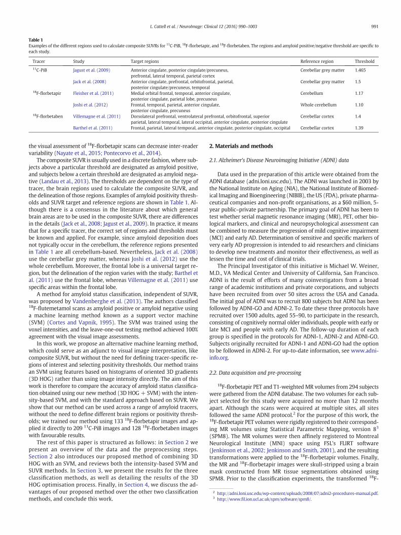
Table 1Examples of the different regions used to calculate composite SUVRs for 11C-PiB, 18F-florbetapir, and 18F-florbetaben. The regions and amyloid positive/negative threshold are specific toeach study.

Tracer Study Target regions Reference region Threshold

11C-PiB Jagust et al. (2009) Anterior cingulate, posterior cingulate/precuneus,prefrontal, lateral temporal, parietal cortex

Cerebellar grey matter 1.465

Jack et al. (2008) Anterior cingulate, prefrontal, orbitofrontal, parietal,posterior cingulate/precuneus, temporal

Cerebellar grey matter 1.5

18F-florbetapir Fleisher et al. (2011) Medial orbital frontal, temporal, anterior cingulate,posterior cingulate, parietal lobe, precuneus

Cerebellum 1.17

Joshi et al. (2012) Frontal, temporal, parietal, anterior cingulate,posterior cingulate, precuneus

Whole cerebellum 1.10

18F-florbetaben Villemagne et al. (2011) Dorsolateral prefrontal, ventrolateral prefrontal, orbitofrontal, superiorparietal, lateral temporal, lateral occipital, anterior cingulate, posterior cingulate

Cerebellar cortex 1.4

Barthel et al. (2011) Frontal, parietal, lateral temporal, anterior cingulate, posterior cingulate, occipital Cerebellar cortex 1.39

2 http://adni.loni.usc.edu/wp-content/uploads/2008/07/adni2-procedures-manual.pdf.3 http://www.fil.ion.ucl.ac.uk/spm/software/spm8/.

991L. Cattell et al. / NeuroImage: Clinical 12 (2016) 990–1003

the visual assessment of 18F-florbetapir scans can decrease inter-readervariability (Nayate et al., 2015; Pontecorvo et al., 2014).

The composite SUVR is usually used in a discrete fashion,where sub-jects above a particular threshold are designated as amyloid positive,and subjects below a certain threshold are designated as amyloid nega-tive (Landau et al., 2013). The thresholds are dependent on the type oftracer, the brain regions used to calculate the composite SUVR, andthe delineation of those regions. Examples of amyloid positivity thresh-olds and SUVR target and reference regions are shown in Table 1. Al-though there is a consensus in the literature about which generalbrain areas are to be used in the composite SUVR, there are differencesin the details (Jack et al., 2008; Jagust et al., 2009). In practice, it meansthat for a specific tracer, the correct set of regions and thresholds mustbe known and applied. For example, since amyloid deposition doesnot typically occur in the cerebellum, the reference regions presentedin Table 1 are all cerebellum-based. Nevertheless, Jack et al. (2008)use the cerebellar grey matter, whereas Joshi et al. (2012) use thewhole cerebellum. Moreover, the frontal lobe is a universal target re-gion, but the delineation of the region varies with the study; Barthel etal. (2011) use the frontal lobe, whereas Villemagne et al. (2011) usespecific areas within the frontal lobe.

A method for amyloid status classification, independent of SUVR,was proposed by Vandenberghe et al. (2013). The authors classified18F-flutemetamol scans as amyloid positive or amyloid negative usinga machine learning method known as a support vector machine(SVM) (Cortes and Vapnik, 1995). The SVM was trained using thevoxel intensities, and the leave-one-out testing method achieved 100%agreement with the visual image assessments.

In this work, we propose an alternative machine learning method,which could serve as an adjunct to visual image interpretation, likecomposite SUVR, but without the need for defining tracer-specific re-gions of interest and selecting positivity thresholds. Our method trainsan SVM using features based on histograms of oriented 3D gradients(3D HOG) rather than using image intensity directly. The aim of thiswork is therefore to compare the accuracy of amyloid status classifica-tion obtained using our new method (3D HOG+ SVM) with the inten-sity-based SVM, and with the standard approach based on SUVR. Weshow that our method can be used across a range of amyloid tracers,without the need to define different brain regions or positivity thresh-olds; we trained our method using 133 18F-florbetapir images and ap-plied it directly to 209 11C-PiB images and 128 18F-florbetaben imageswith favourable results.

The rest of this paper is structured as follows: in Section 2 wepresent an overview of the data and the preprocessing steps.Section 2 also introduces our proposed method of combining 3DHOG with an SVM, and reviews both the intensity-based SVM andSUVR methods. In Section 3, we present the results for the threeclassification methods, as well as detailing the results of the 3DHOG optimisation process. Finally, in Section 4, we discuss the ad-vantages of our proposed method over the other two classificationmethods, and conclude this work.

2. Materials and methods

2.1. Alzheimer's Disease Neuroimaging Initiative (ADNI) data

Data used in the preparation of this article were obtained from theADNI database (adni.loni.usc.edu). The ADNI was launched in 2003 bythe National Institute on Aging (NIA), the National Institute of Biomed-ical Imaging and Bioengineering (NIBIB), the US (FDA), private pharma-ceutical companies and non-profit organisations, as a $60 million, 5-year public–private partnership. The primary goal of ADNI has been totest whether serial magnetic resonance imaging (MRI), PET, other bio-logical markers, and clinical and neuropsychological assessment canbe combined to measure the progression of mild cognitive impairment(MCI) and early AD. Determination of sensitive and specific markers ofvery early AD progression is intended to aid researchers and cliniciansto develop new treatments and monitor their effectiveness, as well aslessen the time and cost of clinical trials.

The Principal Investigator of this initiative is Michael W. Weiner,M.D., VA Medical Center and University of California, San Francisco.ADNI is the result of efforts of many coinvestigators from a broadrange of academic institutions and private corporations, and subjectshave been recruited from over 50 sites across the USA and Canada.The initial goal of ADNI was to recruit 800 subjects but ADNI has beenfollowed by ADNI-GO and ADNI-2. To date these three protocols haverecruited over 1500 adults, aged 55–90, to participate in the research,consisting of cognitively normal older individuals, people with early orlate MCI and people with early AD. The follow-up duration of eachgroup is specified in the protocols for ADNI-1, ADNI-2 and ADNI-GO.Subjects originally recruited for ADNI-1 and ADNI-GO had the optionto be followed in ADNI-2. For up-to-date information, see www.adni-info.org.

2.2. Data acquisition and pre-processing

18F-florbetapir PET and T1-weighted MR volumes from 294 subjectswere gathered from the ADNI database. The two volumes for each sub-ject selected for this study were acquired no more than 12 monthsapart. Although the scans were acquired at multiple sites, all sitesfollowed the same ADNI protocol.2 For the purpose of this work, the18F-florbetapir PET volumeswere rigidly registered to their correspond-ing MR volumes using Statistical Parametric Mapping, version 83

(SPM8). The MR volumes were then affinely registered to MontrealNeurological Institute (MNI) space using FSL's FLIRT software(Jenkinson et al., 2002; Jenkinson and Smith, 2001), and the resultingtransformations were applied to the 18F-florbetapir volumes. Finally,the MR and 18F-florbetapir images were skull-stripped using a brainmask constructed from MR tissue segmentations obtained usingSPM8. Prior to the classification experiments, the transformed 18F-

992 L. Cattell et al. / NeuroImage: Clinical 12 (2016) 990–1003

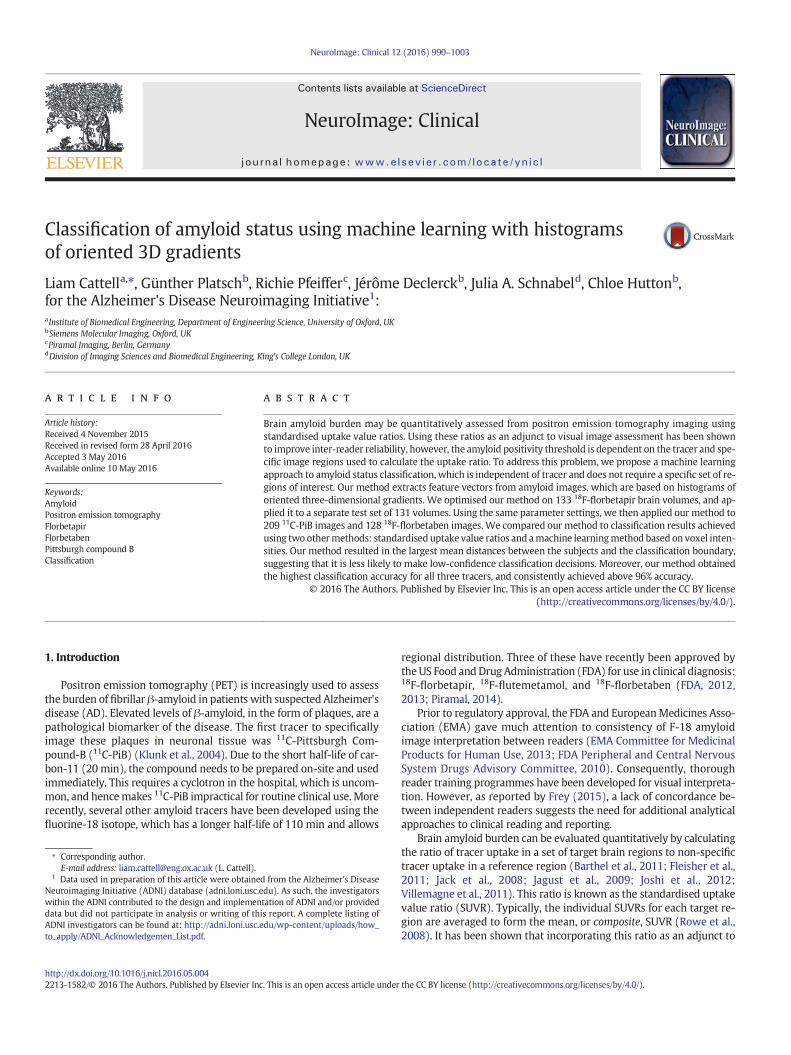
florbetapir PET brain volumes were resampled to 2 × 2 × 2 mm resolu-tion. Axial slices from examples of amyloid negative and amyloid posi-tive 18F-florbetapir brain volumes, along with their corresponding MRslices, are shown in Fig. 1(a).

In addition to the 18F-florbetapir data, 214 11C-PiB and correspond-ing T1-weighted MR volumes were downloaded from the ADNI data-base. The data belonged to 102 subjects, but even though somesubjects had multiple scans (26 subjects had one scan, 42 subjects hadtwo scans, 32 subjects had three scans, and two subjects had fourscans), each 11C-PiB/MR pair was treated independently. Each 11C-PiBvolume and its corresponding MR volume were acquired within12 months of one another. Furthermore, the 11C-PiB scans underwentthe same pre-processing as the 18F-florbetapir volumes. Example amy-loid positive and amyloid negative axial slices from the 11C-PiB datasetare shown in Fig. 1(b).

The 18F-florbetaben PET volumes and corresponding T1-weightedMR volumes were provided from the phase 2A clinical trial of 18F-florbetaben in 150participants. The participant details and imagingpro-tocols are all provided in Barthel et al. (2011). Seventeen subjects wereexcluded due to severe image artefacts in the PET orMR images. TheMRand 18F-florbetaben PET volumes were coregistered using an in-houserigid registration algorithm. The 18F-florbetaben images were then reg-istered to a PET template inMNI space using an in-house affine registra-tion algorithm and resampled to 2 × 2 × 2mm resolution. The in-houserigid and affine registration algorithms were implemented using rou-tines customised fromSiemens syngo.PETAmyloid Plaque (sPAP) quan-tification software. The resulting transformations were applied to theMR volumes. Analogously to the 18F-florbetapir and 11C-PiB, a brainmask was constructed using tissue segmentations obtained fromSPM8. Both the 18F-florbetaben PET volumes and their correspondingMR volumes were skull-stripped. Fig. 1(c) shows an example axialslice for a 18F-florbetaben amyloid negative and 18F-florbetaben amy-loid positive brain volume. The corresponding axial MR slices are alsoshown in Fig. 1(c).

2.3. Visual assessment

In this study, the gold standard amyloid status was determined foreach subject using criteria based on visual assessments from threeimage readers. Data were excluded from the study if the median ratingwas neither amyloid positive nor amyloid negative. To interpret the PETvolumes as amyloid positive or amyloid negative, the three imagereaders (one clinical expert, one senior neuro-PET researcher, and onejunior PET image analysis researcher) interpreted the images a total ofsix times. The junior researcher assessed all of the images three times,the senior neuro-PET researcher interpreted all the images twice, andthe clinical expert read all of the images once. The tracers were assessedone at a time (i.e. all 18F-florbetapir scans were interpreted before the11C-PiB scans), but for each tracer the images were presented in a ran-dom order to prevent observer memory affecting the assessments.Each reader was given instructions on how to display and interpretthe images on a set of prearranged slices, without access to the corre-sponding MR image. For the 18F-florbetapir and 18F-florbetaben scans,the instructions were based on those provided by the tracer manufac-turers (Amyvid, 2012; NeuraCeq, 2014). The only major differencewas the addition of an “equivocal” image class, for images that did notclearly fulfil the definitions of positive or negative scans. Note thatsince the reading instructions were very thorough, “equivocal” wastypically only selected when image quality was particularly poor. Theinstructions for visual assessment of 11C-PiB were based on a combina-tion of those by Suotunen et al. (2010) and Cohen et al. (2013). Again, anequivocal image class was included for images that could not be desig-nated as either amyloid positive or amyloid negative.

Using Fleiss' kappa to assess the inter-reader reliability, the siximage interpretations showed substantial agreement for all tracers(18F-florbetapir: κ=0.71, 11C-PiB: κ=0.81, 18F-florbetaben: κ=0.84).

The gold standard amyloid status was determined from the median ofthe six image interpretations. Any images for which the median inter-pretationwas not amyloid positive or amyloid negativewere discarded.In total, 30 18F-florbetapir images, five 11C-PiB images, and five 18F-florbetaben images were discarded. The final 18F-florbetapir datasetcomprised 264 subjects, the final 11C-PiB dataset consisted of 209 sub-jects, and the final 18F-florbetaben dataset contained 128 subjects. Thedemographics of these are summarised in Table 2. It should be notedthat although the inter-reader agreement and number of equivocalscans varies by tracer, this is not a reflection of the tracers themselves.The discrepancies are predominantly due to differences in image qualityand the distributions of amyloid burden.

2.4. Image analysis

In this work we compared three separate amyloid classificationmethods: our method, which uses histograms of oriented three-dimen-sional gradients as inputs to an SVM (3D HOG + SVM), another SVM-based method using image intensity directly, and SUVR. The threemethods are outlined in Sections 2.5–2.7.

2.5. Histogram of oriented 3D gradients (3D HOG)

2.5.1. Derivation of feature vectorsImage descriptors have been widely used in computer vision to de-

scribe characteristics such as texture, motion, and shapes in imagesand video sequences (Belongie and Malik, 2000; Dalal and Triggs,2005; Lowe, 1999). Given a region of interest, a descriptor representsthe region as a feature vector. By applyingmachine learning techniquesto these feature vectors, they can be used to detect objects in images.One such method, histogram of oriented gradients (HOG), has beenused successfully to detect pedestrians in static images (Dalal andTriggs, 2005). The image is partitioned into a grid of uniformly spacedcells, and the normalised histogram of image gradient orientations ineach cell forms the set of feature vectors. An illustration of HOG in twodimensions is shown in Fig. 2. The key concepts of this two-dimensionalmethod were generalised to three dimensions by Kläser et al. (2008).Although originally used for action recognition in video volumes, wehere propose to apply a similar technique to PET volumes to classifybrain amyloid status.

In order to compute histograms of oriented gradients across a PETvolume, the volume is partitioned into a uniform grid of cells ci of sizek×k×k voxels. Each cell is divided into S×S×S sub-blocks bj, and foreach sub-block the mean gradient is computed. In the same manneras Kläser et al. (2008), we calculated the mean gradient using a 3D ex-tension of the integral image (also known as a summed area table),popularised by Viola and Jones (2001). Given a volume v(x,y,z) and its

gradient ∇v ¼ ð∂v∂x ; ∂v∂y ; ∂v∂zÞT, the integral volume can be written as:

I x; y; zð Þ ¼X

x0 ≤ x;y0 ≤y;z0 ≤ z∇v x0; y0; z0ð Þ: ð1Þ

The mean 3D gradient g ¼ ðgx; gy; gzÞT within a cuboid of sizew×h×d at position (x,y,z)T is then given by:

g ¼ I xþw; yþ h; zþ dð Þ−I x; yþ h; zþ dð Þð−I xþw; y; zþ dð Þ þ I x; y; zþ dð ÞÞ− I xþw; yþ h; zð Þ−I x; yþ h; zð Þð−I xþw; y; zð Þ þ I x; y; zð ÞÞ:

ð2Þ

Following computation of the 3D gradient g , its orientation isquantised into a histogram with n discrete bins. A logical extension ofthe 2D HOG method would be to use spherical polar coordinates toquantise the 3D gradient orientations. By dividing the elevation angleand azimuth into equally sized bins, gradients are quantised using a

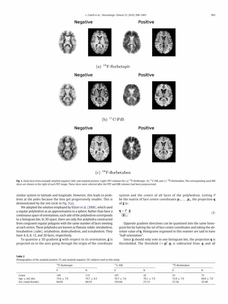
Fig. 1. Axial slices from example amyloid negative (left) and amyloid positive (right) PET volumes for (a) 18F-florbetapir, (b) 11C-PiB, and (c) 18F-florbetaben. The corresponding axial MRslices are shown to the right of each PET image. These slices were selected after the PET and MR volumes had been preprocessed.

993L. Cattell et al. / NeuroImage: Clinical 12 (2016) 990–1003

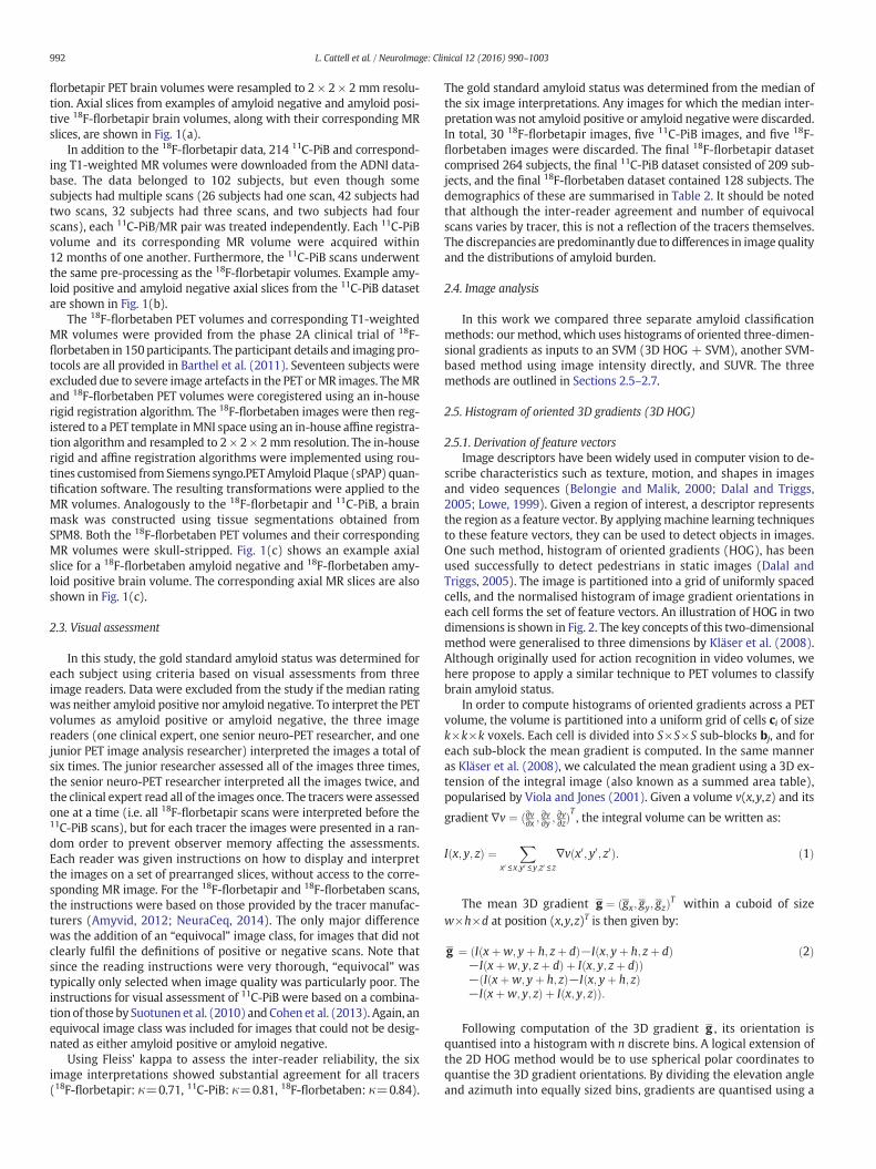
similar system to latitude and longitude. However, this leads to prob-lems at the poles because the bins get progressively smaller. This isdemonstrated by the red circle in Fig. 3(a).

We adopted the solution employed by Kläser et al. (2008),which useda regular polyhedron as an approximation to a sphere. Rather than have acontinuous space of orientations, each side of thepolyhedron correspondsto a histogram bin. In 3D space, there are only five polyhedra constructedfrom congruent regular polygonswith the same number of facesmeetingat each vertex. Thesepolyhedra are knownas Platonic solids: tetrahedron,hexahedron (cube), octahedron, dodecahedron, and icosahedron. Theyhave 4, 6, 8, 12, and 20 faces, respectively.

To quantise a 3D gradient g with respect to its orientation, g isprojected on to the axes going through the origin of the coordinate

Table 2Demographics of the amyloid positive (P) and amyloid negative (N) subjects used in this stud

18F-florbetapir 11C-

P N P

Count 149 115 167Age ± std. dev. 75.6 ± 7.6 74.7 ± 8.5 76.7Sex (male/female) 84/65 60/55 103

system and the centre of all faces of the polyhedron. Letting Pbe the matrix of face centre coordinates p1 , … ,pn, the projection qof g is:

q ¼ P � ggk k2:

ð3Þ

Opposite gradient directions can be quantised into the same histo-grambin by halving the set of face centre coordinates and taking the ab-solute value of q. Histograms organised in this manner are said to have“half-orientation”.

Since g should only vote in one histogram bin, the projection q isthresholded. The threshold t=pi

T ⋅pj is subtracted from q and all

y.

PiB 18F-florbetaben

N P N

42 53 75± 7.6 76.1 ± 7.4 72.0 ± 7.9 69.0 ± 7.0/64 27/15 27/26 35/40

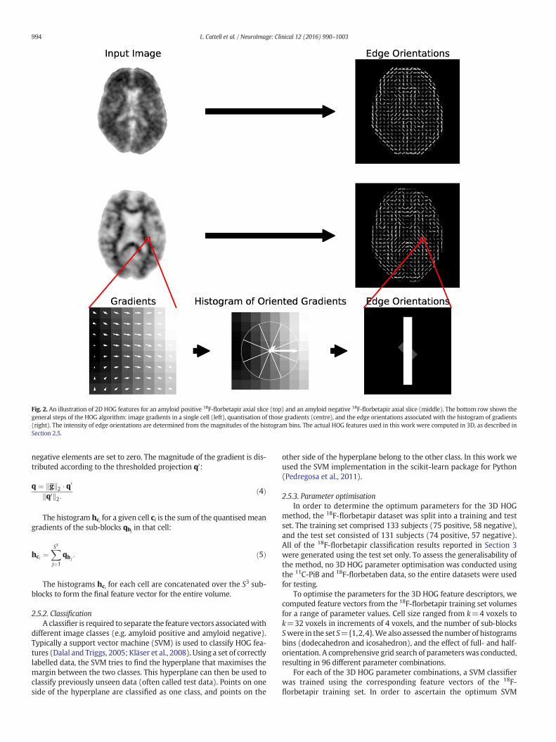
Fig. 2. An illustration of 2D HOG features for an amyloid positive 18F-florbetapir axial slice (top) and an amyloid negative 18F-florbetapir axial slice (middle). The bottom row shows thegeneral steps of the HOG algorithm: image gradients in a single cell (left), quantisation of those gradients (centre), and the edge orientations associated with the histogram of gradients(right). The intensity of edge orientations are determined from the magnitudes of the histogram bins. The actual HOG features used in this work were computed in 3D, as described inSection 2.5.

994 L. Cattell et al. / NeuroImage: Clinical 12 (2016) 990–1003

negative elements are set to zero. The magnitude of the gradient is dis-tributed according to the thresholded projection q0:

q ¼ gk k2 � q0

q0k k2:ð4Þ

The histogram hci for a given cell ci is the sum of the quantisedmeangradients of the sub-blocks qbj

in that cell:

hci ¼XS3

j¼1

qb j: ð5Þ

The histograms hci for each cell are concatenated over the S3 sub-blocks to form the final feature vector for the entire volume.

2.5.2. ClassificationA classifier is required to separate the feature vectors associatedwith

different image classes (e.g. amyloid positive and amyloid negative).Typically a support vector machine (SVM) is used to classify HOG fea-tures (Dalal and Triggs, 2005; Kläser et al., 2008). Using a set of correctlylabelled data, the SVM tries to find the hyperplane that maximises themargin between the two classes. This hyperplane can then be used toclassify previously unseen data (often called test data). Points on oneside of the hyperplane are classified as one class, and points on the

other side of the hyperplane belong to the other class. In this work weused the SVM implementation in the scikit-learn package for Python(Pedregosa et al., 2011).

2.5.3. Parameter optimisationIn order to determine the optimum parameters for the 3D HOG

method, the 18F-florbetapir dataset was split into a training and testset. The training set comprised 133 subjects (75 positive, 58 negative),and the test set consisted of 131 subjects (74 positive, 57 negative).All of the 18F-florbetapir classification results reported in Section 3were generated using the test set only. To assess the generalisability ofthe method, no 3D HOG parameter optimisation was conducted usingthe 11C-PiB and 18F-florbetaben data, so the entire datasets were usedfor testing.

To optimise the parameters for the 3D HOG feature descriptors, wecomputed feature vectors from the 18F-florbetapir training set volumesfor a range of parameter values. Cell size ranged from k=4 voxels tok=32 voxels in increments of 4 voxels, and the number of sub-blocksSwere in the set S={1,2,4}.We also assessed thenumber of histogramsbins (dodecahedron and icosahedron), and the effect of full- and half-orientation. A comprehensive grid search of parameterswas conducted,resulting in 96 different parameter combinations.

For each of the 3D HOG parameter combinations, a SVM classifierwas trained using the corresponding feature vectors of the 18F-florbetapir training set. In order to ascertain the optimum SVM

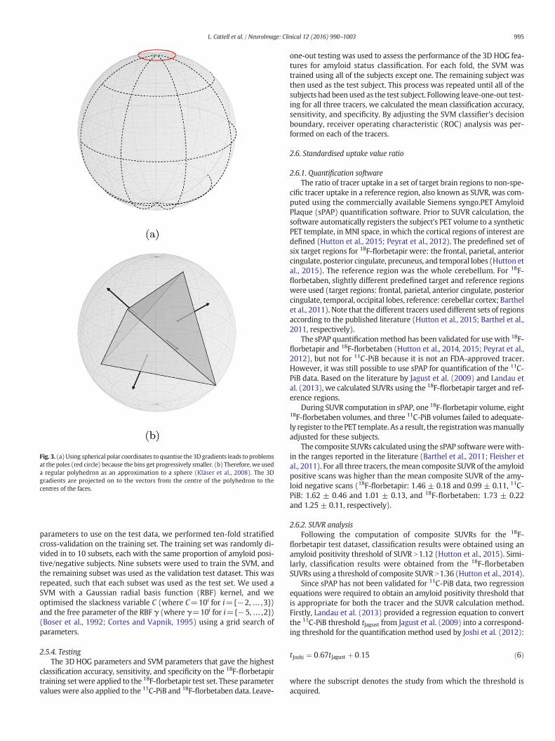
Fig. 3. (a)Using spherical polar coordinates to quantise the 3Dgradients leads to problemsat the poles (red circle) because the bins get progressively smaller. (b) Therefore, we useda regular polyhedron as an approximation to a sphere (Kläser et al., 2008). The 3Dgradients are projected on to the vectors from the centre of the polyhedron to thecentres of the faces.

995L. Cattell et al. / NeuroImage: Clinical 12 (2016) 990–1003

parameters to use on the test data, we performed ten-fold stratifiedcross-validation on the training set. The training set was randomly di-vided in to 10 subsets, each with the same proportion of amyloid posi-tive/negative subjects. Nine subsets were used to train the SVM, andthe remaining subset was used as the validation test dataset. This wasrepeated, such that each subset was used as the test set. We used aSVM with a Gaussian radial basis function (RBF) kernel, and weoptimised the slackness variable C (where C=10i for i={−2,… ,3})and the free parameter of the RBF γ (where γ=10i for i={−5,… ,2})(Boser et al., 1992; Cortes and Vapnik, 1995) using a grid search ofparameters.

2.5.4. TestingThe 3D HOG parameters and SVM parameters that gave the highest

classification accuracy, sensitivity, and specificity on the 18F-florbetapirtraining setwere applied to the 18F-florbetapir test set. These parametervalues were also applied to the 11C-PiB and 18F-florbetaben data. Leave-

one-out testing was used to assess the performance of the 3D HOG fea-tures for amyloid status classification. For each fold, the SVM wastrained using all of the subjects except one. The remaining subject wasthen used as the test subject. This process was repeated until all of thesubjects had been used as the test subject. Following leave-one-out test-ing for all three tracers, we calculated the mean classification accuracy,sensitivity, and specificity. By adjusting the SVM classifier's decisionboundary, receiver operating characteristic (ROC) analysis was per-formed on each of the tracers.

2.6. Standardised uptake value ratio

2.6.1. Quantification softwareThe ratio of tracer uptake in a set of target brain regions to non-spe-

cific tracer uptake in a reference region, also known as SUVR, was com-puted using the commercially available Siemens syngo.PET AmyloidPlaque (sPAP) quantification software. Prior to SUVR calculation, thesoftware automatically registers the subject's PET volume to a syntheticPET template, in MNI space, in which the cortical regions of interest aredefined (Hutton et al., 2015; Peyrat et al., 2012). The predefined set ofsix target regions for 18F-florbetapir were: the frontal, parietal, anteriorcingulate, posterior cingulate, precuneus, and temporal lobes (Hutton etal., 2015). The reference region was the whole cerebellum. For 18F-florbetaben, slightly different predefined target and reference regionswere used (target regions: frontal, parietal, anterior cingulate, posteriorcingulate, temporal, occipital lobes, reference: cerebellar cortex; Barthelet al., 2011). Note that the different tracers used different sets of regionsaccording to the published literature (Hutton et al., 2015; Barthel et al.,2011, respectively).

The sPAP quantificationmethod has been validated for use with 18F-florbetapir and 18F-florbetaben (Hutton et al., 2014, 2015; Peyrat et al.,2012), but not for 11C-PiB because it is not an FDA-approved tracer.However, it was still possible to use sPAP for quantification of the 11C-PiB data. Based on the literature by Jagust et al. (2009) and Landau etal. (2013), we calculated SUVRs using the 18F-florbetapir target and ref-erence regions.

During SUVR computation in sPAP, one 18F-florbetapir volume, eight18F-florbetaben volumes, and three 11C-PiB volumes failed to adequate-ly register to the PET template. As a result, the registrationwasmanuallyadjusted for these subjects.

The composite SUVRs calculated using the sPAP softwarewerewith-in the ranges reported in the literature (Barthel et al., 2011; Fleisher etal., 2011). For all three tracers, themean composite SUVR of the amyloidpositive scans was higher than the mean composite SUVR of the amy-loid negative scans (18F-florbetapir: 1.46 ± 0.18 and 0.99 ± 0.11, 11C-PiB: 1.62 ± 0.46 and 1.01 ± 0.13, and 18F-florbetaben: 1.73 ± 0.22and 1.25 ± 0.11, respectively).

2.6.2. SUVR analysisFollowing the computation of composite SUVRs for the 18F-

florbetapir test dataset, classification results were obtained using anamyloid positivity threshold of SUVR N1.12 (Hutton et al., 2015). Simi-larly, classification results were obtained from the 18F-florbetabenSUVRs using a threshold of composite SUVR N1.36 (Hutton et al., 2014).

Since sPAP has not been validated for 11C-PiB data, two regressionequations were required to obtain an amyloid positivity threshold thatis appropriate for both the tracer and the SUVR calculation method.Firstly, Landau et al. (2013) provided a regression equation to convertthe 11C-PiB threshold tJagust from Jagust et al. (2009) into a correspond-ing threshold for the quantification method used by Joshi et al. (2012):

tJoshi ¼ 0:67tJagust þ 0:15 ð6Þ

where the subscript denotes the study from which the threshold isacquired.

996 L. Cattell et al. / NeuroImage: Clinical 12 (2016) 990–1003

Hutton et al. (2015) also provided a regression equation to convertfrom the Joshi et al. (2012) method threshold into an equivalent unitfor sPAP tsPAP:

tsPAP ¼ 0:9782tJoshi þ 0:04264: ð7Þ

We can combine Eqs. (6) and (7) to get a final equation to convertbetween the 11C-PiB threshold tJagust and sPAP tsPAP:

tsPAP ¼ 0:9782 0:67tJagust þ 0:15� �þ 0:04264

≃0:6554tJagust þ 0:1894: ð8Þ

By substituting tJagust=1.465 (Jagust et al., 2009) into Eq. (8), we getan equivalent threshold for 11C-PiB in sPAP tsPAP=1.15. Consequently,following SUVR calculation in sPAP, the accuracy of amyloid status clas-sification in 11C-PiB data was assessed using an amyloid positivitythreshold of composite SUVR N1.15.

2.7. Image intensity

We compared our method and SUVR to themachine learningmeth-od proposed by Vandenberghe et al. (2013). In that work, the authorstrained a SVM on voxel intensity to classify amyloid positivity in 18F-flutemetamol images. Each image is a point in high-dimensionalspace, in which each dimension is a voxel within the brain.

To reduce the dimension of the SVM, only voxels inside the brainwere used. Once all of the images were transformed into MNI space(see Section 2.2), we constructed a brain mask using the linearMNI152 T1-weighted MR template (Mazziotta et al., 2001). The maskwas dilated by 2 mm to ensure that all of the registered PET brainswere wholly inside the mask. Prior to using the SVM, all of the imageswere normalised to have zeromean and unit variance. The SVM param-eters were then optimised using the same approach as in Section 2.5.3.The optimum parameters were applied to the 18F-florbetapir test data,as well as the 11C-PiB and 18F-florbetaben datasets. Leave-one-out test-ingwas used to assess the ability of the intensity-based SVMs to classifyamyloid status.

Fig. 4. The highest classification accuracies achieved for each of the 96 3D HOG parameter combvs. icosahedron, and half-orientation vs. full-orientation), and shows the highest classification acparameter combinations, highlighted in red, achieved the same, highest classification accuracy

3. Results

3.1. 3D HOG parameter optimisation

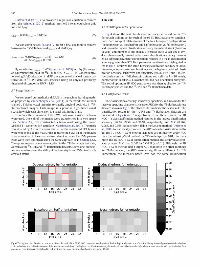
Fig. 4 shows the best classification accuracies achieved on the 18F-florbetapir training set for each of the 96 3D HOG parameter combina-tions. Each sub-plot relates to one of the four histogram configurations(dodecahedron vs. icosahedron, and half-orientation vs. full-orientation),and shows the highest classification accuracy for each cell size k (horizon-tal axis) and number of sub-blocks S (vertical axis). A cell size of k=4voxels universally resulted in the lowest classification accuracy. Howev-er, 68 different parameter combinations resulted in a mean classificationaccuracy greater than 95%. Four parameter combinations (highlighted inred in Fig. 4) achieved the same, highest classification accuracy of 98.5%.However, one parameter combination gave the highest combined classi-fication accuracy, sensitivity, and specificity (98.5%, 0.973, and 1.00, re-spectively) on the 18F-florbetapir training set: cell size k=16 voxels,number of sub-blocks S=1, icosahedron, and half-orientation histogram.This set of optimum 3D HOG parameters was then applied to the 18F-florbetapir test set, and the 11C-PiB and 18F-florbetaben data.

3.2. Classification results

The classification accuracy, sensitivity, specificity and area under thereceiver operating characteristic curve (AUC) for the 18F-florbetapir testdata are shown in Fig. 5. The black borders indicate the best results. Theclassification results for the 11C-PiB and 18F-florbetaben datasets arepresented in Figs. 6 and 7, respectively. For all three tracers, the 3DHOG + SVM classification method resulted in the largest classificationaccuracy (96.2%, 99.5%, and 96.9%, respectively) and AUC (0.962,0.988, and 0.965, respectively). Using the DeLong method (DeLong etal., 1988) to statistically compare the AUCs of each classification meth-od, the 3D HOG + SVM method achieved a significantly larger AUCthan the intensity-SVM method for 18F-florbetapir (pb0.01). Further-more, the 3D HOG + SVM classification method also achieved a signif-icantly larger AUC than SUVR for 11C-PiB (pb0.01). Although the 3DHOG + SVM method had a larger AUC than both the other methodsfor 18F-florbetaben, the AUCs were not significantly different. For 18F-florbetaben, the intensity-based SVM had the same classification

inations. Each sub-plot relates to one of the four histogram configurations (dodecahedroncuracy for each cell size k (horizontal axis) and number of sub-blocks S (vertical axis). Four(98.5%).

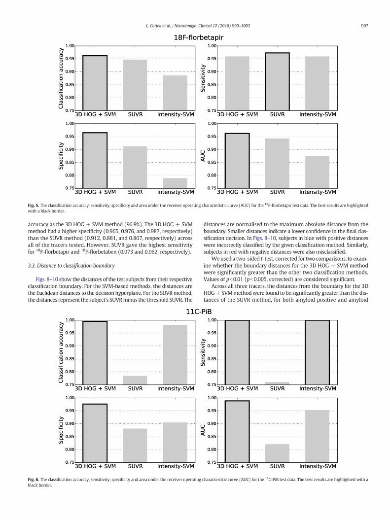
Fig. 5. The classification accuracy, sensitivity, specificity and area under the receiver operating characteristic curve (AUC) for the 18F-florbetapir test data. The best results are highlightedwith a black border.

997L. Cattell et al. / NeuroImage: Clinical 12 (2016) 990–1003

accuracy as the 3D HOG + SVM method (96.9%). The 3D HOG + SVMmethod had a higher specificity (0.965, 0.976, and 0.987, respectively)than the SUVR method (0.912, 0.881, and 0.867, respectively) acrossall of the tracers tested. However, SUVR gave the highest sensitivityfor 18F-florbetapir and 18F-florbetaben (0.973 and 0.962, respectively).

3.3. Distance to classification boundary

Figs. 8–10 show the distances of the test subjects from their respectiveclassification boundary. For the SVM-based methods, the distances arethe Euclidean distances to the decision hyperplane. For the SUVRmethod,the distances represent the subject's SUVRminus the threshold SUVR. The

Fig. 6. The classification accuracy, sensitivity, specificity and area under the receiver operatingblack border.

distances are normalised to the maximum absolute distance from theboundary. Smaller distances indicate a lower confidence in the final clas-sification decision. In Figs. 8–10, subjects in blue with positive distanceswere incorrectly classified by the given classification method. Similarly,subjects in red with negative distances were also misclassified.

We used a two-sided t-test, corrected for two comparisons, to exam-ine whether the boundary distances for the 3D HOG + SVM methodwere significantly greater than the other two classification methods.Values of pb0.01 (pb0.005, corrected) are considered significant.

Across all three tracers, the distances from the boundary for the 3DHOG+SVMmethodwere found to be significantly greater than the dis-tances of the SUVR method, for both amyloid positive and amyloid

characteristic curve (AUC) for the 11C-PiB test data. The best results are highlighted with a

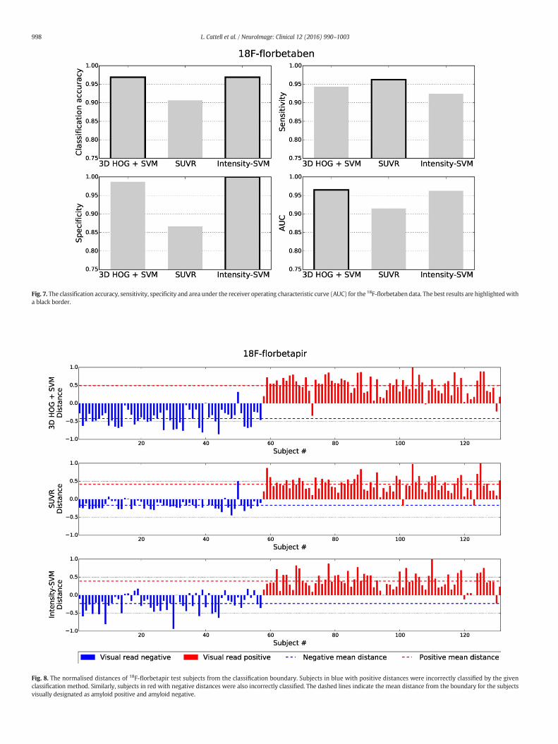
Fig. 7. The classification accuracy, sensitivity, specificity and area under the receiver operating characteristic curve (AUC) for the 18F-florbetaben data. The best results are highlightedwitha black border.

Fig. 8. The normalised distances of 18F-florbetapir test subjects from the classification boundary. Subjects in blue with positive distances were incorrectly classified by the givenclassification method. Similarly, subjects in red with negative distances were also incorrectly classified. The dashed lines indicate the mean distance from the boundary for the subjectsvisually designated as amyloid positive and amyloid negative.

998 L. Cattell et al. / NeuroImage: Clinical 12 (2016) 990–1003

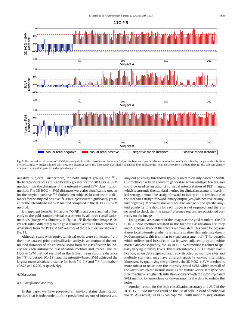
Fig. 9. The normalised distances of 11C-PiB test subjects from the classification boundary. Subjects in blue with positive distances were incorrectly classified by the given classificationmethod. Similarly, subjects in red with negative distances were also incorrectly classified. The dashed lines indicate the mean distance from the boundary for the subjects visuallydesignated as amyloid positive and amyloid negative.

999L. Cattell et al. / NeuroImage: Clinical 12 (2016) 990–1003

negative subjects. Furthermore, for both subject groups, the 18F-florbetapir distances are significantly greater for the 3D HOG + SVMmethod than the distances of the intensity-based SVM classificationmethod. The 3D HOG + SVM distances were also significantly greaterfor the amyloid positive 18F-florbetaben subjects. In contrast, the dis-tances for the amyloid positive 11C-PiB subjectswere significantly great-er for the intensity-based SVMmethod compared to the 3DHOG+SVMmethod.

It is apparent from Fig. 9 that one 11C-PiB imagewas classified differ-ently to the gold standard visual assessment by all three classificationmethods (image #9). Similarly, in Fig. 10, 18F-florbetaben image #104was classified differently to the gold standard across all three methods.Axial slices from the PET andMR volumes of these outliers are shown inFig. 11.

Although scans with equivocal visual reads were eliminated fromthe three datasets prior to classification analysis, we computed the nor-malised distances of the equivocal scans from the classification bound-ary for each automated classification method and tracer. The 3DHOG + SVM method resulted in the largest mean absolute distancefor 18F-florbetapir (0.418), and the intensity-based SVM achieved thelargest mean absolute distance for both 11C-PiB and 18F-florbetaben(0.878 and 0.700, respectively).

4. Discussion

4.1. Classification accuracy

In this paper we have proposed an amyloid status classificationmethod that is independent of the predefined regions of interest and

amyloid positivity thresholds typically used to classify based on SUVR.Our method has been shown to generalise across multiple tracers, andcould be used as an adjunct to visual interpretation of PET images,which is currently the standardmethod for clinical assessment. In a clin-ical setting, it would be straightforward to interpret the results due tothe method's straightforward, binary output (amyloid positive or amy-loid negative). Moreover, unlike SUVR, knowledge of the specific amy-loid positivity thresholds for each tracer is not required, and there isno need to check that the target/reference regions are positioned cor-rectly on the image.

Using visual assessment of the images as the gold standard, the 3DHOG + SVM method resulted in the highest classification accuracyand AUC for all three of the tracers we evaluated. This could be becauseit uses local intensity gradients as features, rather than intensity direct-ly. Conceptually, this is similar to visual assessment of 18F-florbetapir,which utilises local loss of contrast between adjacent grey and whitematter, and consequently, the 3D HOG+ SVMmethod is robust to spa-tially varying intensity levels. This is advantageous in PET image classi-fication, when data acquired, and reconstructed, at multiple sites andmultiple scanners, may have different spatially varying intensities.Moreover, by quantising the gradients, the 3D HOG + SVM method ismore robust to noise than the intensity-based SVM, which uses all ofthe voxels, which can include noise, as the feature vector. Itmay be pos-sible to achieve a higher classification accuracywith the intensity-basedSVM method by smoothing or downsampling the data to reduce thenoise.

Another reason for the high classification accuracy and AUC of the3D HOG + SVM method could be the use of cells, instead of individualvoxels. As a result, 3D HOG can cope well with minor misregistration

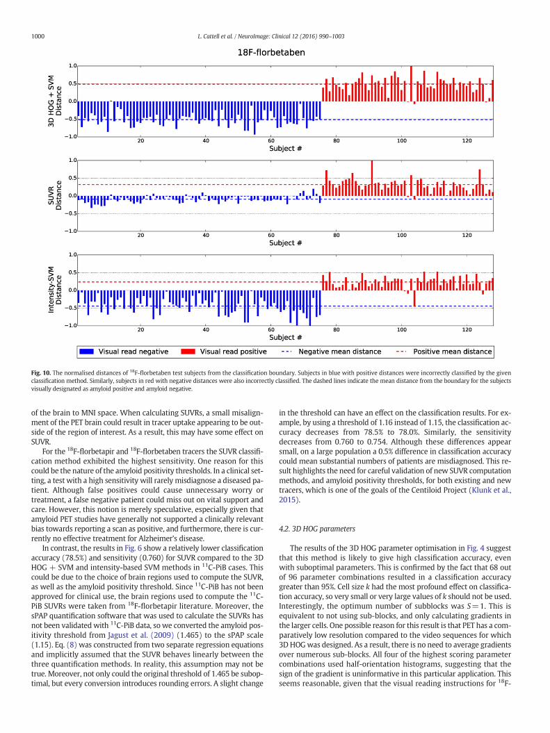
Fig. 10. The normalised distances of 18F-florbetaben test subjects from the classification boundary. Subjects in blue with positive distances were incorrectly classified by the givenclassification method. Similarly, subjects in red with negative distances were also incorrectly classified. The dashed lines indicate the mean distance from the boundary for the subjectsvisually designated as amyloid positive and amyloid negative.

1000 L. Cattell et al. / NeuroImage: Clinical 12 (2016) 990–1003

of the brain to MNI space. When calculating SUVRs, a small misalign-ment of the PET brain could result in tracer uptake appearing to be out-side of the region of interest. As a result, this may have some effect onSUVR.

For the 18F-florbetapir and 18F-florbetaben tracers the SUVR classifi-cation method exhibited the highest sensitivity. One reason for thiscould be the nature of the amyloid positivity thresholds. In a clinical set-ting, a test with a high sensitivity will rarely misdiagnose a diseased pa-tient. Although false positives could cause unnecessary worry ortreatment, a false negative patient could miss out on vital support andcare. However, this notion is merely speculative, especially given thatamyloid PET studies have generally not supported a clinically relevantbias towards reporting a scan as positive, and furthermore, there is cur-rently no effective treatment for Alzheimer's disease.

In contrast, the results in Fig. 6 show a relatively lower classificationaccuracy (78.5%) and sensitivity (0.760) for SUVR compared to the 3DHOG + SVM and intensity-based SVM methods in 11C-PiB cases. Thiscould be due to the choice of brain regions used to compute the SUVR,as well as the amyloid positivity threshold. Since 11C-PiB has not beenapproved for clinical use, the brain regions used to compute the 11C-PiB SUVRs were taken from 18F-florbetapir literature. Moreover, thesPAP quantification software that was used to calculate the SUVRs hasnot been validated with 11C-PiB data, so we converted the amyloid pos-itivity threshold from Jagust et al. (2009) (1.465) to the sPAP scale(1.15). Eq. (8) was constructed from two separate regression equationsand implicitly assumed that the SUVR behaves linearly between thethree quantification methods. In reality, this assumption may not betrue. Moreover, not only could the original threshold of 1.465 be subop-timal, but every conversion introduces rounding errors. A slight change

in the threshold can have an effect on the classification results. For ex-ample, by using a threshold of 1.16 instead of 1.15, the classification ac-curacy decreases from 78.5% to 78.0%. Similarly, the sensitivitydecreases from 0.760 to 0.754. Although these differences appearsmall, on a large population a 0.5% difference in classification accuracycould mean substantial numbers of patients are misdiagnosed. This re-sult highlights the need for careful validation of new SUVR computationmethods, and amyloid positivity thresholds, for both existing and newtracers, which is one of the goals of the Centiloid Project (Klunk et al.,2015).

4.2. 3D HOG parameters

The results of the 3D HOG parameter optimisation in Fig. 4 suggestthat this method is likely to give high classification accuracy, evenwith suboptimal parameters. This is confirmed by the fact that 68 outof 96 parameter combinations resulted in a classification accuracygreater than 95%. Cell size k had the most profound effect on classifica-tion accuracy, so very small or very large values of k should not be used.Interestingly, the optimum number of subblocks was S=1. This isequivalent to not using sub-blocks, and only calculating gradients inthe larger cells. One possible reason for this result is that PET has a com-paratively low resolution compared to the video sequences for which3D HOGwas designed. As a result, there is no need to average gradientsover numerous sub-blocks. All four of the highest scoring parametercombinations used half-orientation histograms, suggesting that thesign of the gradient is uninformative in this particular application. Thisseems reasonable, given that the visual reading instructions for 18F-

Fig. 11. PET and MR axial slices from the two images which were classified differently tothe gold standard visual assessment by all three classification methods. (a) 11C-PiBimage #9 was visually assessed as amyloid negative, but incorrectly classified aspositive. However, on closer inspection, tracer uptake was observed in the frontal region(highlighted by the red box), suggesting that the classification should be amyloidpositive. (b) 18F-florbetaben image #104 was correctly assessed as positive, butautomatically classified as amyloid negative.

1001L. Cattell et al. / NeuroImage: Clinical 12 (2016) 990–1003

florbetaben state that the images should be displayed in grey scale or in-verse grey scale (NeuraCeq, 2014).

4.3. Distance from the classification boundary

For all cases except positive 11C-PiB subjects, the 3D HOG + SVMmethod resulted in the greatest mean distances from the decisionboundary. A large distance is desirable, since points near the classifica-tion boundary represent low-confidence classification decisions.Again, one reason for the superior performance of the 3D HOG + SVMmethod could be that it utilises image gradients, rather than directvoxel intensities. The resulting invariance to spatially varying intensitylevels and noise robustness allows the two populations to be more eas-ily separated than using SUVR or the intensity-based SVM method.

The small distance between amyloid negative subjects and the SUVRthreshold supports its relatively lower specificity in Figs. 5–7. The sub-jects close to the threshold are classified with a lower confidence, andare more likely to be misclassified as false positives.

The two images that were classified differently to the gold standardvisual assessment (11C-PiB image #9 and 18F-florbetaben image #104)were visually assessed again by two of the original three readers. Al-though the 18F-florbetaben image was again assessed to be an amyloidpositive subject by the readers, the distance from the classificationboundary for the SUVR and 3D HOG + SVM classification methods

was small. This indicates that the different automatic classification deci-sion has low confidence, and that this subject is a particularly difficultborderline case. After visual reassessment of the 11C-PiB case, forwhich the gold standard amyloid status was negative, a small regionof tracer uptake was identified in the frontal lobe (highlighted by thered box in Fig. 11(a)), suggesting that the gold standard amyloid statusmay have been incorrect for this case. This highlights the importance ofusing an adjunct to visual assessment of amyloid images. In this study,the visual reads were conducted using PET volumes only. However,using MR images to help localise tracer uptake might make visual as-sessment more robust.

In this study, scans were given an “equivocal” visual assessment ifthey did not clearly fulfil the stringent definitions of amyloid positiveor amyloid negative scans. Typically, scans were only designated asequivocal when readers lacked confidence in a final classification dueto poor image quality. For this reason, equivocal scans are the type ofscans forwhich automated classification could bemost useful. Althoughthere is no gold standard to which the classification results can be com-pared, the distances of the equivocal scans from the boundary indicatethe level of confidence in the final classification of the automated classi-fication methods. The 3D HOG + SVM method achieved the largestmean absolute distance from the boundary (0.418) for the equivocal18F-florbetapir scans, suggesting a higher level of confidence in thefinal classification than the SUVR and intensity-based SVM methods.For the equivocal 11C-PiB and 18F-florbetaben scans, the intensity-based SVM method resulted in the largest mean absolute distancefrom the classification boundary (0.878 and 0.700, respectively). How-ever, due to the small sample size (only five equivocal scans for both11C-PiB and 18F-florbetaben), the distances for the intensity-basedSVMmethodwere not significantly larger (pb0.01) than those achievedby the other two classification methods.

4.4. Methodological considerations

In this study, the gold standard for amyloid status was determinedusing criteria based on consistent visual assessments from three imagereaders. Although ADNI provides a clinical diagnosis (e.g. cognitivelynormal, mild cognitive impairment, Alzheimer's disease) for each sub-ject at the time of the 18F-florbetapir and 11C-PiB scans, these diagnosesare determined using a range of clinical tests. Consequently, the visualinterpretations of the scans may not correlate with the clinical diagno-ses (Frey, 2015). For example, a subject with an amyloid negative scanmay not be clinically diagnosed as a healthy control. Since the methodsemployed in this paper focus on classification of amyloid status usingPET images only, the clinical diagnoses from ADNI were discarded.Moreover, the tracer manufacturer instructions state that a positive18F-florbetapir scan does not establish a diagnosis of Alzheimer's diseaseor other cognitive disorder (Amyvid, 2012).

For this study, the gold standard amyloid status for each scan wasobtained using the median rating from six visual assessments by threedifferent image readers. The most junior reader interpreted the imagesthree times and the most senior reader assessed the images once. Al-though the number of evaluations varied for each reader, this had littleeffect on the final gold standard visual assessments and classificationexperiments. For example, if the first assessment from each readerwere used, such that each reader only contributed one data point perscan, the gold standard classification would change for only six 11C-PiBscans and two 18F-florbetaben scans. The median visual assessmentfor both 18F-florbetaben scans would change from amyloid negative toequivocal, thus excluding the scans from our study, and reducing thesize of the dataset. Similarly, four of the 11C-PiB scans would bereclassified as equivocal scans. The median visual assessment of the re-maining two 11C-PiB scanswould change from amyloid negative to am-yloid positive. Although the gold standard classification would changefor 17 18F-florbetapir scans if the first visual assessment from each read-er were used, the median rating of all 17 scans would change to

1002 L. Cattell et al. / NeuroImage: Clinical 12 (2016) 990–1003

equivocal. Consequently, these 17 scans would have been excludedfrom this work, and therefore the effect on the classification accuraciespresented in Section 3.2 would be minimal.

In this work, we optimised the 3DHOGparameters and SVMparam-eters completely independently of the test data. We optimised the 3DHOG + SVM parameters using the 18F-florbetapir training data, andused a leave-one-out testing approach on the test data for all threetracers. Since the 3D HOG + SVM parameters were optimised using18F-florbetapir data only, the entire 11C-PiB and 18F-florbetaben datasetswere used for testing. Therefore, leave-one-out testingwas used so thatthe SVMclassifierwas always trained using data from the same amyloidPET tracer as the test data. However, if the SVM that is applied to the testdata is trained using the original 18F-florbetapir training data,4 the clas-sification accuracies for the 3D HOG + SVM method are only slightlylower than using leave-one-out testing (18F-florbetapir: 90.8%, 11C-PiB: 96.7%, 18F-florbetaben: 93.8%). In contrast, if the same approach isused to test the intensity-based SVM method, the classification accura-cies are considerably lower than using leave-one-out testing (18F-florbetapir: 56.5%, 11C-PiB: 79.9%, 18F-florbetaben: 41.4%).

In future, to fully assess the generalisability of the 3D HOG + SVMmethod, we need to analyse the classification results obtained byoptimising the 3D HOG parameters on other amyloid PET tracers than18F-florbetapir. This is the subject of ongoing research, and for clarity,we chose not to present our results here. Nevertheless, our preliminaryresults indicate that the 3D HOG + SVM method can achieve a higherclassification accuracy than SUVR and the intensity-based SVMmethod,regardless of the amyloid PET tracer used to optimise the 3D HOGparameters.

Although we used all of the 11C-PiB and 18F-florbetaben data thatwere available to us, the ADNI database contains many more 18F-florbetapir scans than were used in this work. Therefore, in future, itwould be useful to test our method on a larger dataset.

Prior to computing the 3D HOG feature vectors, we affinely regis-tered the PET volumes to MNI space to ensure that the cells generallycontained the same brain regions across all subjects. We could haveused a deformable registration algorithm, however, to keep thepre-pro-cessing steps of our method in line with the sPAP SUVR method, affineregistration was used. Furthermore, it has been shown that classifica-tion of Alzheimer's disease patients versus cognitively normal controlsusing SUVR is not affected by the registrationmethod (affine versus de-formable registration) (Cattell et al., 2015).

Many other feature descriptors have been developed in addition tohistograms of oriented gradients. For example, the Scale-Invariant Fea-ture Transform (SIFT) algorithm has been successfully used for objectrecognition in computer vision tasks (Lowe, 1999), and has also beenused in feature-based morphometry in MRI to distinguish between pa-tients with Alzheimer's disease and healthy controls (Toews et al.,2010). Nevertheless, we chose to use 3D HOG features due to their sim-plicity and speed of computation. Moreover, unlike SIFT and SpeededUp Robust Features (SURF) (Bay et al., 2006), HOG operates on adense grid of cells rather than individual points of interest. A larger setof image descriptors over a dense grid will typically offermore informa-tion than similar descriptors evaluated at a sparse set of image points.

Unlike the original intensity-based SVM method proposed byVandenberghe et al. (2013), which used a SVM with a linear kernel,we used a SVMwith aGaussian radial basis function kernel. Our primaryreason for using a non-linear kernel was because the subjects in theoriginal input space of the SVM might not be linearly separable. Al-though a linear SVM is faster to compute, and non-linear kernels cangive rise to overfitting, it has been shown that if complete model selec-tion using the Gaussian kernel has been conducted, there is no need toconsider a linear SVM (Keerthi and Lin, 2003). In this work, we

4 i.e. If a leave-one-out testing approach is not used, and the SVM used to classify the11C-PiB and 18F-florbetaben data is trained using 18F-florbetapir data.

optimised the parameters of the SVM and Gaussian kernel on the 18F-florbetapir training data only, using a grid search of parameters.

On a practical level, our 3D HOG + SVM method uses less memorythan the intensity-based SVMmethod. The 3DHOG feature vector com-prised 1500 elements, whereas the feature vector for the intensity-based method contained an element for each voxel inside the brainmask (290,409 elements in total). As the number of elements increases,so does the time taken to train the SVM. The SUVR is also very quick tocompute, but unlike ourmethod, knowledge of the underlying anatomyand disease pathology is required in order to choose suitable target andreference regions.

4.5. Conclusion

In this paper we have proposed a machine learning method foramyloid status classification based on histograms of oriented three-dimensional gradients. We compared our method to SUVRs obtainedfrom clinically validated amyloid quantification software, as well as an-other machine learning method based solely on image intensity(Vandenberghe et al., 2013). Across three separate amyloid tracers,our method achieved the highest classification accuracy and areaunder the receiver operating characteristic curve. Unlike SUVR, our 3DHOG + SVMmethod required very little recalibration between tracers,andwe showed that ourmethod has the potential to produce satisfacto-ry results even with suboptimal parameters. Moreover, the large sepa-ration between the population groups suggests that our methodmakes fewer low-confidence classification decisions. In addition, inthe future, we plan to specify a band of indecision on either side of theclassification boundary to give visual readers a measure of confidencein the automatic classification, as well as their own classificationdecision.

Acknowledgements

This work was funded by an Industrial CASE award grant from theEngineering and Physical Sciences Research Council (grant number:11440394), with sponsorship from Siemens Molecular Imaging. Wewould like to thank Piramal Imaging for supplying the 18F-florbetabendata, and corresponding MR images used in this study.

Data collection and sharing for this project was funded by theAlzheimer's Disease Neuroimaging Initiative (ADNI) (National Insti-tutes of Health Grant U01 AG024904) and DOD ADNI (Department ofDefense award number W81XWH-12-2-0012). ADNI is funded by theNational Institute on Aging, theNational Institute of Biomedical Imagingand Bioengineering, and through generous contributions from the fol-lowing: AbbVie, Alzheimer's Association; Alzheimer's Drug DiscoveryFoundation; Araclon Biotech; BioClinica, Inc.; Biogen; Bristol-MyersSquibb Company; CereSpir, Inc.; Eisai Inc.; Elan Pharmaceuticals, Inc.;Eli Lilly and Company; EuroImmun; F. Hoffmann-La Roche Ltd. and itsaffiliated company Genentech, Inc.; Fujirebio; GE Healthcare; IXICOLtd.; Janssen Alzheimer Immunotherapy Research & Development,LLC.; Johnson & Johnson Pharmaceutical Research & DevelopmentLLC.; Lumosity; Lundbeck; Merck & Co., Inc.; Meso Scale Diagnostics,LLC.; NeuroRx Research; Neurotrack Technologies; Novartis Pharma-ceuticals Corporation; Pfizer Inc.; Piramal Imaging; Servier; TakedaPharmaceutical Company; and Transition Therapeutics. The CanadianInstitutes of Health Research is providing funds to support ADNI clinicalsites in Canada. Private sector contributions are facilitated by the Foun-dation for the National Institutes of Health (www.fnih.org). The granteeorganisation is theNorthern California Institute for Research and Educa-tion, and the study is coordinated by the Alzheimer's Disease Coopera-tive Study at the University of California, San Diego. ADNI data aredisseminated by the Laboratory for Neuro Imaging at the University ofSouthern California.

1003L. Cattell et al. / NeuroImage: Clinical 12 (2016) 990–1003

References

Amyvid, 2012. Amyvid (florbetapir F 18 injection) highlights of prescribing information.http://www.accessdata.fda.gov/drugsatfda_docs/label/2012/202008s000lbl.pdf (Apr,Accessed: Jul 15, 2015).

Barthel, H., Gertz, H.J., Dresel, S., Peters, O., Bartenstein, P., Buerger, K., Hiemeyer, F.,Wittemer-Rump, S.M., Seibyl, J., Reininger, C., Sabri, O., 2011. Cerebral amyloid-βPETwith florbetaben (18F) in patients with Alzheimer's disease and healthy controls:a multicentre phase 2 diagnostic study. Lancet Neurol. 10 (5), 424–435 (May).

Bay, H., Tuytelaars, T., Van Gool, L., 2006. SURF: speeded up robust features. ECCV 2006vol. 3951, pp. 404–417.

Belongie, S., Malik, J., 2000. Matching with shape contexts. CBAIVL 2000, pp. 20–26 (Jun).Boser, B.E., Guyon, I.M., Vapnik, V.N., 1992. A training algorithm for optimal margin clas-

sifiers. COLT 1992, pp. 144–152.Cattell, L., Schnabel, J.A., Declerck, J., Hutton, C., 2015. Investigation of single- versus joint-

modality PET–MR registration for 18F-florbetapir quantification: application toAlzheimer's disease. Computational Methods for Molecular Imaging, Volume 22 ofLecture Notes in Computational Vision and Biomechanics. Springer International Pub-lishing, pp. 197–205.

Cohen, A.D., Mowrey, W., Weissfeld, L.A., Aizenstein, H.J., McDade, E., Mountz, J.M., Nebes,R.D., Saxton, J.A., Snitz, B., DeKosky, S., Williamson, J., Lopez, O.L., Price, J.C., Mathis,C.A., Klunk, W.E., 2013. Classification of amyloid-positivity in controls: comparisonof visual read and quantitative approaches. NeuroImage 71, 207–215.

Cortes, C., Vapnik, V., 1995. Support-vector networks. Mach. Learn. 20 (3), 273–297 (Sep).Dalal, N., Triggs, D., 2005. Histograms of oriented gradients for human detection. CVPR

2005 vol. 1, pp. 886–893 (Jun).DeLong, E.R., DeLong, D.M., Clarke-Pearson, D.L., 1988. Comparing the areas under two or

more correlated receiver operating characteristic curves: a nonparametric approach.Biometrics 44 (3), 837–845.

EMA Committee for Medicinal Products for Human Use, 2013. Public assessment report:NeuraCeq florbetaben 18 F. http://www.ema.europa.eu/docs/en_GB/document_library/EPAR_-_Public_assessment_report/human/002553/WC500162593.pdf (Dec,Accessed: Jul 14, 2015).

FDA, 2012. FDA approves 18F-florbetapir PET agent. J. Nucl. Med. 53 (6), 15N.FDA, 2013. FDA press release: Vizamyl approval. http://www.fda.gov/NewsEvents/

Newsroom/PressAnnouncements/ucm372261.htm (Oct, Accessed: Jul 24, 2015).FDA Peripheral and Central Nervous System Drugs Advisory Committee, 2010o.

FDA advisory committee briefing document: new drug application 202-008Amyvid (florbetapir F 18 injection). http://www.fda.gov/downloads/Advisory%20Committees/CommitteesMeetingMaterials/Drugs/Peripheraland%20CentralNervousSystemDrugsAdvisoryCommittee/UCM240265.pdf (Dec,Accessed: Jul 14, 2015).

Fleisher, A.S., Chen, K., Liu, X., Roontiva, A., Thiyyagura, P., Ayutyanont, N., Joshi, A.D.,Clark, C.M., Mintun, M.A., Pontecorvo, M.J., Doraiswamy, P.M., Johnson, K.A.,Skovronsky, D.M., Reiman, E.M., 2011. Using positron emission tomography andflorbetapir F18 to image cortical amyloid in patients with mild cognitive impairmentor dementia due to Alzheimer disease. Arch. Neurol. 68 (11), 1404–1411.

Frey, K.A., 2015. Amyloid imaging in dementia: contribution or confusion? J. Nucl. Med.56 (3), 331–333.

Hutton, C., Declerck, J., Mintun, M., Pontecorvo, M.J., Devous Sr., M.D., Joshi, A.D., 2015.Quantification of 18F-florbetapir PET: comparison of two analysis methods. Eur.J. Nucl. Med. Mol. Imaging 42 (5), 725–732 (Apr).

Hutton, C., Sibille, L., Bullich, S., Catafau, A., Koglin, N., Pfeiffer, R., Declerck, J., 2014. Com-parison of two methods, with and without MRI, for quantification of florbetaben(18F) PET. EANM 2014 (Oct).

Jack Jr., C.R., Lowe, V.J., Senjem, M.L., Weigand, S.D., Kemp, B.J., Shiung, M.M., Knopman,D.S., Boeve, B.F., Klunk, W.E., Mathis, C.A., Petersen, R.C., 2008. 11C PiB and structuralMRI provide complementary information in imaging of Alzheimer's disease andamnestic mild cognitive impairment. Brain 131 (Pt3), 665–680 (Mar).

Jagust, W.J., Landau, S.M., Shaw, L.M., Trojanowski, J.Q., Koeppe, R.A., Reiman, E.M., Foster,N.L., Petersen, R.C., Weiner, M.W., Price, J.C., Mathis, C.A., 2009. Relationships betweenbiomarkers in aging and dementia. Neurology 73 (15), 1193–1199.

Jenkinson, M., Smith, S.M., 2001. A global optimisation method for robust affine registra-tion of brain images. Med. Image Anal. 5 (2), 143–156.

Jenkinson, M., Bannister, P.R., Brady, J.M., Smith, S.M., 2002. Improved optimisation for therobust and accurate linear registration and motion correction of brain images.NeuroImage 17 (2), 825–841.

Joshi, A.D., Pontecorvo, M.J., Clark, C.M., Carpenter, A.P., Jennings, D.L., Sadowsky, C.H.,Adler, L.P., Kovnat, K.D., Seibyl, J.P., Arora, A., Saha, K., Burns, J.D., Lowrey, M.J.,Mintun, M.A., Skovronsky, D.M., 2012. Performance characteristics of amyloid PET

with florbetapir F 18 in patients withAlzheimer's disease and cognitively normal sub-jects. J. Nucl. Med. 53 (3), 378–384 (Mar).

Keerthi, S.S., Lin, C., 2003. Asymptotic behaviors of support vector machines with Gauss-ian kernel. Neural Comput. 15 (7), 1667–1689.

Kläser, A., Marszalek, M., Schmid, C., 2008. A spatio-temporal descriptor based on 3D-gra-dients. BMVC 2008, pp. 1–10 (Sep).

Klunk, W.E., Engler, H., Nordberg, A., Wang, Y., Blomqvist, G., Holt, D.P., Bergstrom, M.,Savitcheva, I., Huang, G.F., Estrada, S., Ausen, B., Debnath, M.L., Barletta, J., Price, J.C.,Sandell, J., Lopresti, B.J., Wall, A., Koivisto, P., Antoni, G., Mathis, C.A., Langstrom, B.,2004. Imaging brain amyloid in Alzheimer's disease with Pittsburgh Compound-B.Ann. Neurol. 55 (3), 306–319 (Mar).

Klunk, W.E., Koeppe, R.A., Price, J.C., Benzinger, T.L., Devous Sr., M.D., Jagust, W.J., Johnson,K.A., Mathis, C.A., Minhas, D., Pontecorvo, M.J., Rowe, C.C., Skovronsky, D.M., Mintun,M.A., 2015. The Centiloid Project: standardizing quantitative amyloid plaque estima-tion by PET. Alzheimers Dement. 11 (1), 1–15 (Jan).

Landau, S.M., Breault, C., Joshi, A.D., Pontecorvo, M., Mathis, C.A., Jagust, W.J., Mintun, M.A.,2013. Amyloid-β imaging with Pittsburgh Compound B and florbetapir: comparingradiotracers and quantification methods. J. Nucl. Med. 54 (1), 70–77.

Lowe, D.G., 1999. Object recognition from local scale-invariant features. ICCV 1999 vol. 2,pp. 1150–1157 (Sep).

Mazziotta, J.C., Toga, A.W., Evans, A.C., Fox, P.T., Lancaster, J., Zilles, K., Woods, R., Paus, T.,Simpson, G., Pike, B., Holmes, C.J., Collins, D.L., Thompson, P., MacDonald, D., Iacoboni,M., Schormann, T., Amunts, K., Palomero-Gallagher, N., Geyer, S., Parson, L., Narr, K.,Kabani, N., LeGoualher, G., Boomsma, D., Cannon, T., Kawashima, R., Mazoyer, B.,2001. Four-dimensional probabilistic atlas of the human brain. J. Am. Med. Inform.Assoc. 8 (5), 401–430.

Nayate, A.P., Dubroff, J.G., Schmitt, J.E., Nasrallah, I., Kishore, R., Mankoff, D., Pryma, D.A.,2015. Use of standardized uptake value ratios decreases interreader variability of18F florbetapir PET brain scan interpretation. Am. J. Neuroradiol. 1–8.

NeuraCeq, 2014. NEURACEQ (florbetaben F 18 injection) highlights of prescribing informa-tion. http://www.accessdata.fda.gov/drugsatfda_docs/nda/2014/204677Orig1s000Lbl.pdf (Mar, Accessed: Jul 15, 2015).

Pedregosa, F., Varoquaux, G., Gramfort, A., Michel, V., Thirion, B., Grisel, O., Blondel, M.,Prettenhofer, P., Weiss, R., Dubourg, V., Vanderplas, J., Passos, A., Cournapeau, D.,Brucher, M., Perrot, M., Duchesnay, E., 2011. Scikit-learn: machine learning in Python.J. Mach. Learn. Res. 12, 2825–2830.

Peyrat, J.-M., Joshi, A., Mintun, M., Declerck, J., 2012. An automatic method for the quan-tification of uptake with florbetapir imaging. J. Nucl. Med. 53 (Suppl. 1), 210 (May).

Piramal, 2014. FDA approves Piramal Imaging's NeuraCeq (florbetaben F18 injection) forPET imaging of beta-amyloid neuritic plaques in the brain. http://www.piramal.com/imaging/pdf/FDA-Approval-Press-Release.pdf (Mar, Accessed: Jul 24, 2015).

Pontecorvo, M., Devous, M., Arora, A., Devine, M., Lu, M., Joshi, A., Breault, C., Skovronsky,D., Mintun, M., Heun, S., 2014. Can incorporation of a quantitative estimate of corticalto cerebellar SUVr as an adjunct to visual interpretation improve the accuracy and re-liability of florbetapir PET scan interpretation? J. Nucl. Med. Meet. Abstr. 55 (1), 245.

Rowe, C.C., Ackerman, U., Browne, W., Mulligan, R., Pike, K.L., O'Keefe, G., Tochon-Danguy,H., Chan, G., Berlangieri, S.U., Jones, G., Dickinson-Rowe, K.L., Kung, H.P., Zhang, W.,Kung, M.P., Skovronsky, D., Dyrks, T., Holl, G., Krause, S., Friebe, M., Lehman, L.,Lindemann, S., Dinkelborg, L.M., Masters, C.L., Villemagne, V.L., 2008. Imaging of am-yloid beta in Alzheimer's disease with 18F-BAY94-9172, a novel PET tracer: proof ofmechanism. Lancet Neurol. 7 (2), 129–135 (Feb).

Suotunen, T., Hirvonen, J., Immonen-Räihä, P., Aalto, S., Lisinen, I., Arponen, E., Teräs, M.,Koski, K., Sulkava, R., Seppänen, M., Rinne, J.O., 2010. Visual assessment of [11C]PIBPET in patients with cognitive impairment. Eur. J. Nucl. Med. Mol. Imaging 37 (6),1141–1147.

Toews, M., Wells III, W.M., Collins, D.L., Arbel, T., 2010. Feature-based morphometry: dis-covering group-related anatomical patterns. NeuroImage 49 (3), 2318–2327.

Vandenberghe, R., Nelissen, N., Salmon, E., Ivanoiu, A., Hasselbalch, S., Andersen, A.,Korner, A., Minthon, L., Brooks, D.J., Van Laere, K., Dupont, P., 2013. Binary classifica-tion of (18)F-flutemetamol PET using machine learning: comparison with visualreads and structural MRI. NeuroImage 64, 517–525.

Villemagne, V.L., Ong, K., Mulligan, R.S., Holl, G., Pejoska, S., Jones, G., O'Keefe, G.,Ackerman, U., Tochon-Danguy, H., Chan, J.G., Reininger, C.B., Fels, L., Putz, B., Rohde,B., Masters, C.L., Rowe, C.C., 2011. Amyloid imaging with (18)F-florbetaben inAlzheimer disease and other dementias. J. Nucl. Med. 52 (8), 1210–1217 (Aug).

Viola, P., Jones, M., 2001. Rapid object detection using a boosted cascade of simple fea-tures. CVPR 2001.