Journal of Theoretical and Applied Computer Science Vol. 6, No. 2, 2012 RAINFALL TIME SERIES FORECASTING BASED ON MODULAR RBF NEURAL NETWORK MODEL COUPLED WITH SSA AND PLS Jiansheng Wu Yu, Jimin Yu .................................................... 3 TOWARDS EXPERT-BASED MODELLING OF INTEGRATED SOFTWARE QUALITY Lukasz Radliński ........................................................... 13 IS THE CONVENTIONAL INTERVAL-ARITHMETIC CORRECT? Andrzej Piegat, Marek Landowski .............................................. 27 A CLASSIFICATION BASED APPROACH FOR PREDICTING SPRINGBACK IN SHEET METAL FORMING M. Sulaiman Khan, Frans Coenen, Clare Dixon, Subhieh El-Salhi ..................... 45 AUTO-KERNEL USING MULTILAYER PERCEPTRON Wei-Chen Cheng ........................................................... 60 COMPUTER VISION METHODS FOR IMAGE-BASED ARTISTIC IDEATION Ferran Reverter, Pilar Rosado, Eva Figueras, Miquel Àngel Planas .................... 72

Welcome message from author
This document is posted to help you gain knowledge. Please leave a comment to let me know what you think about it! Share it to your friends and learn new things together.
Transcript

Journal of Theoretical and Applied
Computer Science
Vol. 6, No. 2, 2012
RAINFALL TIME SERIES FORECASTING BASED ON MODULAR RBF NEURAL NETWORK MODEL
COUPLED WITH SSA AND PLS
Jiansheng Wu Yu, Jimin Yu . . . . . . . . . . . . . . . . . . . . . . . . . . . . . . . . . . . . . . . . . . . . . . . . . . . . 3
TOWARDS EXPERT-BASED MODELLING OF INTEGRATED SOFTWARE QUALITY
Łukasz Radliński . . . . . . . . . . . . . . . . . . . . . . . . . . . . . . . . . . . . . . . . . . . . . . . . . . . . . . . . . . . 13
IS THE CONVENTIONAL INTERVAL-ARITHMETIC CORRECT?
Andrzej Piegat, Marek Landowski . . . . . . . . . . . . . . . . . . . . . . . . . . . . . . . . . . . . . . . . . . . . . . 27
A CLASSIFICATION BASED APPROACH FOR PREDICTING SPRINGBACK IN SHEET METAL FORMING
M. Sulaiman Khan, Frans Coenen, Clare Dixon, Subhieh El-Salhi . . . . . . . . . . . . . . . . . . . . . 45
AUTO-KERNEL USING MULTILAYER PERCEPTRON
Wei-Chen Cheng . . . . . . . . . . . . . . . . . . . . . . . . . . . . . . . . . . . . . . . . . . . . . . . . . . . . . . . . . . . 60
COMPUTER VISION METHODS FOR IMAGE-BASED ARTISTIC IDEATION
Ferran Reverter, Pilar Rosado, Eva Figueras, Miquel Àngel Planas . . . . . . . . . . . . . . . . . . . . 72

Journal of Theoretical and Applied Computer Science
Scientific quarterly of the Polish Academy of Sciences, The Gdańsk Branch, Computer Science Commission
Scientific advisory board:
Chairman:
Prof. Henryk Krawczyk, Corresponding Member of Polish Academy of Sciences, Gdansk University of Technology, Poland
Members:
Prof. Michał Białko, Member of Polish Academy of Sciences, Koszalin University of Technology, Poland Prof. Aurélio Campilho, University of Porto, Portugal Prof. Ran Canetti, School of Computer Science, Tel Aviv University, Israel Prof. Gisella Facchinetti, Università del Salento, Italy Prof. André Gagalowicz, The National Institute for Research in Computer Science and Control (INRIA), France Prof. Constantin Gaindric, Corresponding Member of Academy of Sciences of Moldova, Institute of Mathematics and Computer Science, Republic of Moldova Prof. Georg Gottlob, University of Oxford, United Kingdom Prof. Edwin R. Hancock, University of York, United Kingdom Prof. Jan Helmke, Hochschule Wismar, University of Applied Sciences, Technology, Business and Design, Wismar, Germany Prof. Janusz Kacprzyk, Member of Polish Academy of Sciences, Systems Research Institute, Polish Academy of Sciences, Poland Prof. Mohamed Kamel, University of Waterloo, Canada Prof. Marc van Kreveld, Utrecht University, The Netherlands Prof. Richard J. Lipton, Georgia Institute of Technology, USA Prof. Jan Madey, University of Warsaw, Poland Prof. Kirk Pruhs, University of Pittsburgh, USA Prof. Elisabeth Rakus-Andersson, Blekinge Institute of Technology, Karlskrona, Sweden Prof. Leszek Rutkowski, Corresponding Member of Polish Academy of Sciences, Czestochowa University of Technology, Poland Prof. Ali Selamat, Universiti Teknologi Malaysia (UTM), Malaysia Prof. Stergios Stergiopoulos, University of Toronto, Canada Prof. Colin Stirling, University of Edinburgh, United Kingdom Prof. Maciej M. Sysło, University of Wrocław, Poland Prof. Jan Węglarz, Member of Polish Academy of Sciences, Poznan University of Technology, Poland Prof. Antoni Wiliński, West Pomeranian University of Technology, Szczecin, Poland Prof. Michal Zábovský, University of Zilina, Slovakia
Editorial board:
Editor-in-chief:
Dariusz Frejlichowski, West Pomeranian University of Technology, Szczecin, Poland
Managing editor:
Piotr Czapiewski, West Pomeranian University of Technology, Szczecin, Poland
Section editors:
Michaela Chocholata, University of Economics in Bratislava, Slovakia Piotr Dziurzański, West Pomeranian University of Technology, Szczecin, Poland Paweł Forczmański, West Pomeranian University of Technology, Szczecin, Poland Przemysław Klęsk, West Pomeranian University of Technology, Szczecin, Poland Radosław Mantiuk, West Pomeranian University of Technology, Szczecin, Poland Jerzy Pejaś, West Pomeranian University of Technology, Szczecin, Poland Izabela Rejer, West Pomeranian University of Technology, Szczecin, Poland
ISSN 2299-2634
The on-line edition of JTACS can be found at: http://www.jtacs.org. The printed edition is to be considered the primary one.
Publisher:
Polish Academy of Sciences, The Gdańsk Branch, Computer Science Commission
Address: Waryńskiego 17, 71-310 Szczecin, Poland
http://www.jtacs.org, email: [email protected]
Journal of Theoretical and Applied Computer Science Vol. 6, No. 2, 2012, pp. 3–12ISSN 2299-2634 http://www.jtacs.org
Rainfall time series forecasting based on Modular RBFNeural Network model coupled with SSA and PLS
Jiansheng Wu YuSchool of Information Engineering, Wuhan University of Technology, P. R. ChinaDepartment of Mathematics and Computer, Liuzhou Teacher College, P. R. [email protected]
Jimin YuSchool of Automation Institute, ChongQing University of Posts and Telecommunications, P. R. ChinaKey Laboratory Network Control and Intelligent Instrument, ChongQing University of Posts and Telecommuni-cations, P. R. [email protected]
Abstract: Accurate forecast of rainfall has been one of the most important issues in hydrological research.Due to rainfall forecasting involves a rather complex nonlinear data pattern; there are lots of novelforecasting approaches to improve the forecasting accuracy. In this paper, a new approach usingthe Modular Radial Basis Function Neural Network (M–RBF–NN) technique is presented to im-prove rainfall forecasting performance coupled with appropriate data–preprocessing techniquesby Singular Spectrum Analysis (SSA) and Partial Least Square (PLS) regression. In the process ofmodular modeling, SSA is applied for the time series extraction of complex trends and structurefinding. In the second stage, the data set is divided into different training sets by Bagging andBoosting technology. In the third stage, the modular RBF–NN predictors are produced by a differ-ent kernel function. In the fourth stage, PLS technology is used to choose the appropriate numberof neural network ensemble members. In the final stage, least squares support vector regressionis used for ensemble of the M–RBF–NN to prediction purpose. The developed RBF–NN modelis being applied for real time rainfall forecasting and flood management in Liuzhou, Guangxi.Aimed at providing forecasts in a near real time schedule, different network types were tested withthe same input information. Additionally, forecasts by M–RBF–NN model were compared to theconvenient approach. Results show that the predictions made using the M–RBF–NN approach areconsistently better than those obtained using the other method presented in this study in terms ofthe same measurements. Sensitivity analysis indicated that the proposed M-RBF-NN techniqueprovides a promising alternative to rainfall prediction.
Keywords: Singular Spectrum Analysis, Radial Basis Function Neural Network, Partial Least Square Regres-sion, Rainfall prediction, Least Squares Support Vector Regression
1. IntroductionAccurate and timely rainfall prediction is essential for planning and management of water
resources, in particular for flood warning systems because it can provide information whichhelp prevent casualties and damage caused by natural disasters [1]. For example, a floodwarning system for fast responding catchments may require a quantitative rainfall forecastto increase the lead time for warning. Similarly, a rainfall forecast provide information inadvance for many water quality problems [2]. Rainfall prediction is one of the most complex
4 Jiansheng Wu Yu, Jimin Yu
elements of the hydrology cycle and at the same time difficult to understand and to model dueto the complexity of the atmospheric processes involved and the variability of rainfall in spaceand time [3], [4].
Although a physically based approach for rainfall forecasting has had several advantagesin recent decades, given the short time scale, the small catchment area, and the massive costsassociated with collecting required meteorological data, it is not a feasible alternative in mostcases. Over the past few decades, many studies have been conducted for the quantitativerainfall forecasting using empirical models including multiple linear regression [5], time seriesmethods [6]and K–nearest–neighbor [7], and data–driven models including artificial neuralnetwork (ANN) [8], support vectors regression (SVR) [9]and fuzzy inference system [10].
Recently, the concept of coupling different models has been a very popular research topicin hydrologic forecasting, which has attracted scientists from other fields including Statistics,Machine Learning and so on. They can be broadly categorized into ensemble models andmodular (or hybrid) models. The basic idea behind ensemble models is to build several differ-ent or similar models for the same process and to integrate them together. Their success largelyarises from the fact that they lead to an improved accuracy compared to a single classificationor regression model. Typically, ensemble methods comprise two phases: a) the productionof multiple predictive models, and b) their combination. In recent work, the reduction of theensemble size has been the main point of concern [11] [12].
In this paper, unlike the previous work, one of the main purposes is to develop a ModularRadial Basis Function Neural Network (MRBF–NN) coupled with appropriate data–prepro-cessing techniques by Singular Spectrum Analysis (SSA) and Partial Least Squar (PLS) toimprove the accuracy of rainfall forecasting. The rainfall data of Liuzhou in Guangxi is pre-dicted as a case study for our proposed method. An actual case of forecasting monthly rainfallis illustrated to show the improvement in predictive accuracy and capability of generalizationachieved by our proposed MRBF–NN model.
The rest of this study is organized as follows. Section 2 describes the proposed MRBF–NN,ideas and procedures. For further illustration, this work employs the method to set up a pre-diction model for rainfall forecasting in Section 3. Discussions are presented in Section 4 andconclusions are drawn in the final Section.
2. The building process of the Modular Radial Basis Function NeuralNetworkFirstly, Singular Spectrum Analysis (SSA) is used to reduce noises in original rainfall
time series, and to reconstruct the new time series in this section. Secondly, a triple–phasenonlinear modular RBF–NN model is proposed for rainfall forecasting based on differentactivation function and training data. Then an appropriate number of RBF–NN predictors areselected from the considerable number of candidate predictors by the Partial Least Squaretechnology. Finally, selected RBF–NN predictors are combined into an aggregated neuralpredictor in terms of LS–SVR.
2.1. Singular Spectrum AnalysisThe Singular Spectrum Analysis (SSA) technique is a novel and powerful technique of
time series analysis incorporating the elements of classical time series analysis, multivariatestatistics, multivariate geometry, dynamical systems and signal processing method. Broom-head and King [13] was presented SSA because they show that the singular value decomposi-
Rainfall time series forecasting based on Modular RBF Neural Network model. . . 5
tion (SVD) is effective in reducing noises. The aim of SSA is to make a decomposition of theoriginal series into the sum of a small number of independent and interpretable componentssuch as a slowly varying trend, oscillatory components and a structure with less noise [14].
The basic SSA algorithm has two stages: decomposition and reconstruction. The de-composition stage requires embedding and singular value decomposition (SVD). Embeddingdecomposes a original time series into the trajectory matrix; SVD turns a trajectory matrixinto the decomposed trajectory matrices which will turn into the trend, seasonal, monthlycomponents, and white noises according to their singular values. The reconstruction stagedemands the grouping to make subgroups of the decomposed trajectory matrices and diago-nal averaging to reconstruct the new time series from the subgroups. The SSA algorithm isdescribed in more detail by the related literature [15] [16].
2.2. Radial Basis Function Neural Network
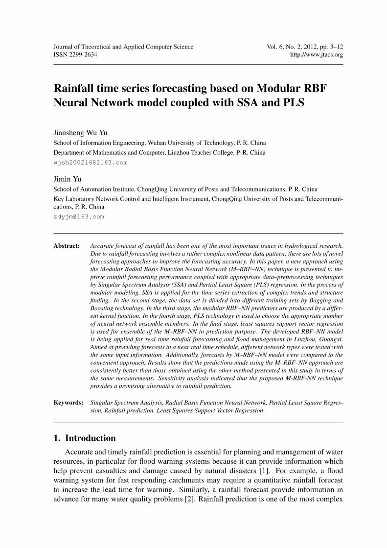
Radial basis function was introduced into the neural network literature by Broomhead andLowe [17] [18], which was motivated by the presence of many local response neurons inhuman brain. On the contrary to the other type of NN used for nonlinear regression, like backpropagation feed forward networks, it learns quickly and has a more compact topology. Thearchitecture is presented in Figure 1.
Figure 1. The RBF–NN architecture
The network is generally composed of three layers: an input layer, a single layer of non-linear processing neuron and output layer. The output of the RBF–NN is calculated accordingto
yi = fi(x) =N∑k=1
wikϕk(∥x− ck∥2), i = 1, 2, · · · ,m (1)
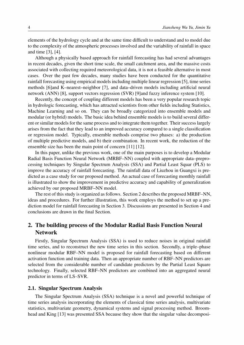
where x ∈ ℜn×1 is an input vector, ϕk(·) is a function from ℜ+ to ℜ, ∥ · ∥2 denotes theEuclidean norm, wik are the weights in the output layer, n is the number of neurons in thehidden layer, and ck ∈ ℜn×1 are the centers in the input vector space. The functional form ofϕk(·) is assumed to have been given, and some typical choices are shown in Table 1.
The training procedure of the RBF networks is a complex process. This procedure re-quires the training of all parameters including the centers of the hidden layer units (ci, i =1, 2, · · · ,m), the widths (σi) of the corresponding Gaussian functions, and the weights (ωi, i =0, 1, · · · ,m) between the hidden layer and output layer. In this paper, the orthogonal leastsquares algorithm (OLS) is used to train RBF based on the minimizing of SSE. More detailedabout the algorithm are provided by the related literature [19].
6 Jiansheng Wu Yu, Jimin Yu
Table 1. Types of kernel function name and formula
Modual Functional name Function formula
A Linear function ϕ(x) = xB Cubic approximation ϕ(x) = x3
C Thin-plate-spline function ϕ(x) = x2lnxD Guassian function ϕ(x) = exp(−x2/σ2)
E Multi-quadratic function ϕ(x) =√x2 + σ2
F Inverse multi-quadratic function ϕ(x) = 1√x2+σ2
2.3. Selecting appropriate ensemble members
When data has completed the training, each Modular RBF-NN predictor has generated itsown result. However, if there is a great number of individual members, we need to select asubset of representatives in order to improve ensemble efficiency. In this paper, the PartialLeast Square (PLS) regression technique is adopted to select appropriate ensemble members.
Partial least squares (PLS) regression analysis was developed in the late seventies by Her-man O. A. Wold [20]. PLS regression is particularly useful when we need to predict a set ofdependent variables from a (very) large set of independent variables (i.e., predictors). Inter-ested readers can be referred to [21] for more details.
2.4. Least Squares Support Vector Regression
Support vector regression (SVR) was derived form support vector machine (SVM) tech-nique. LS–SVM is a least squares modification to the Support Vector Machine [22]. WhenSVM can be used for spectral regression purpose, it is called least squares support vectorregression (LS–SVR). The major advantage of LS–SVM is that it is computationally verycheap while it still possesses some important properties of the SVM. One of the advantages ofLS–SVR is its ability to model nonlinear relationships. In this section we will briefly discussthe LS–SVR method for a regression task. For more detailed information see [23].
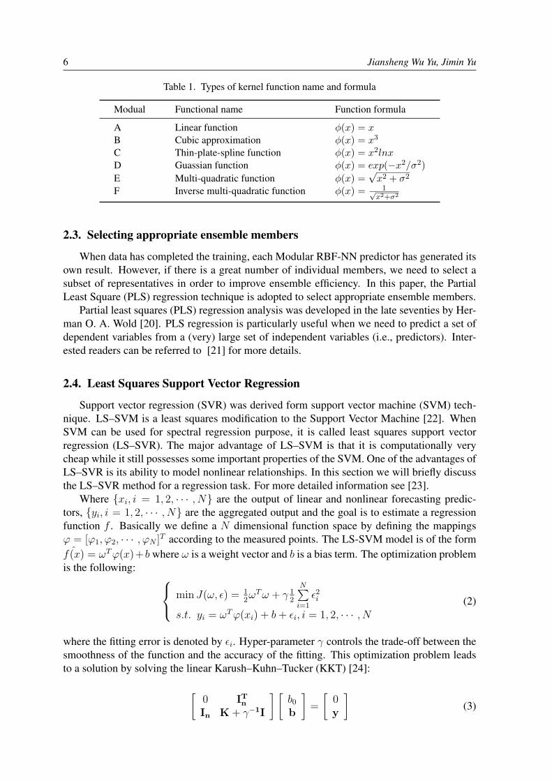
Where {xi, i = 1, 2, · · · , N} are the output of linear and nonlinear forecasting predic-tors, {yi, i = 1, 2, · · · , N} are the aggregated output and the goal is to estimate a regressionfunction f . Basically we define a N dimensional function space by defining the mappingsφ = [φ1, φ2, · · · , φN ]
T according to the measured points. The LS-SVM model is of the formˆf(x) = ωTφ(x)+b where ω is a weight vector and b is a bias term. The optimization problem
is the following: min J(ω, ϵ) = 12ωTω + γ 1
2
N∑i=1
ϵ2i
s.t. yi = ωTφ(xi) + b+ ϵi, i = 1, 2, · · · , N(2)
where the fitting error is denoted by ϵi. Hyper-parameter γ controls the trade-off between thesmoothness of the function and the accuracy of the fitting. This optimization problem leadsto a solution by solving the linear Karush–Kuhn–Tucker (KKT) [24]:
[0 ITnIn K+ γ−1I
] [b0b
]=
[0y
](3)

Rainfall time series forecasting based on Modular RBF Neural Network model. . . 7
where In is a [n × 1] vector of ones, T means transpose of a matrix or vector, γ a weightvector, b regression vector and b0 is the model offset. K is kernel function. A common choicefor the kernel function is the Gaussian function:
K(x, xi) = e∥x−xi∥
2
2σ2 (4)
2.5. The establishment of Modular RBF–NN
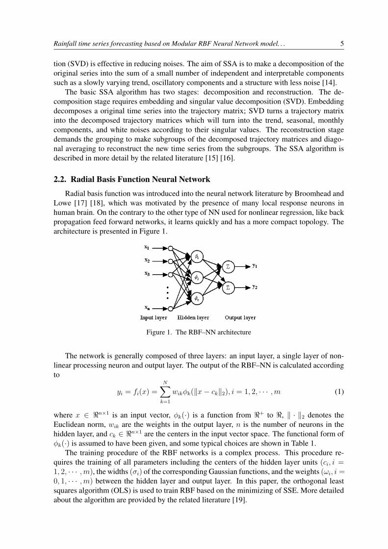
To summarize, the proposed Modular RBF–NN model consists of five main steps. Inthe process of modular modeling, firstly, SSA is applied for the time series extraction ofcomplex trends and structure finding. Secondly, the data set is divided into different trainingsets by using Bagging and Boosting technology. Thirdly, the modular RBF–NN predictorsare produced by a different kernel function. Fourthly, PLS technology is used to choosethe appropriate number of neural network ensemble members. Finally, LS–SVR is used forensemble of the M-RBF-NN to predict purpose. The basic flowchart diagram can be shownin Figure 2.
S S A P r e p r o c e s s i n g
B a g g i n g T e c h n o l o g y
T r a i n i n g S e t T R 1
R B F 1 O u t p u t
P L S S e l e c t i o n g
T r a i n i n g S e t T R 2
T r a i n i n g S e t T R M - 1
T r a i n i n g S e t T R M
R B F 3 O u t p u t
R B F 5 O u t p u t
R B F 6 O u t p u t
R B F 2 O u t p u t
R B F 4 O u t p u t
R a i n f a l l T i m e S e r i e s
L S - S V R E n s e m b l e
Figure 2. The Flowchart of the Modular RBF–NN
3. Results and discussion
3.1. Empirical data
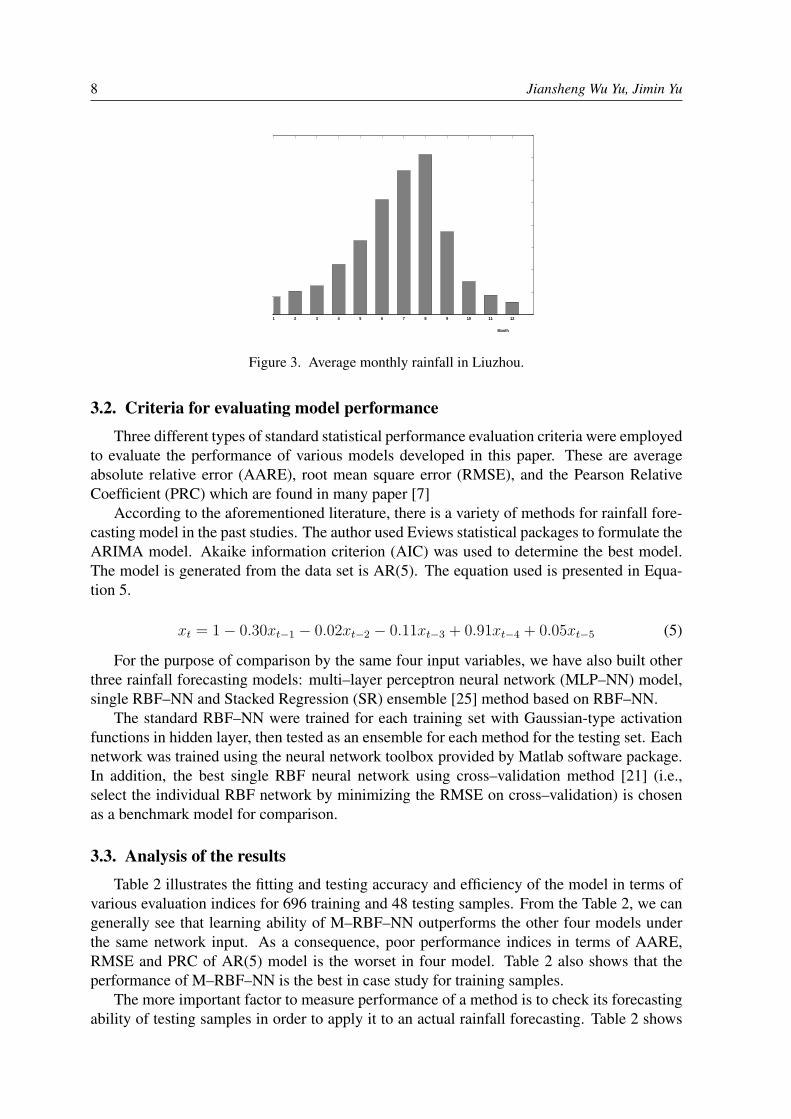
Liuzhou is one of the highly developing cities in southwest of China, and the capital andcommercial city of Guangxi. Historical monthly rainfall data was collected from 24 stationsof the Liuzhou Meteorology Administration (LMA) rain gauge networks for the period from1949 to 2010. After analyzing data, the period from January 1949 to December 2006 wasselected to train MRBF-NN models, and the data from January 2007 to December 2010 wereused as a testing set. Thus the training data set contained 696 data points in time series forMRBF–NN learning, and the other 48 data were used to test sample for MRBF–NN Gener-alization ability. Fig.3 shows the average monthly rainfall, taken over a period from 1949 to2010, in Liuzhou. There is one peak of rainfall during a year, in August.
8 Jiansheng Wu Yu, Jimin Yu
1 2 3 4 5 6 7 8 9 10 11 12
Month
Figure 3. Average monthly rainfall in Liuzhou.
3.2. Criteria for evaluating model performanceThree different types of standard statistical performance evaluation criteria were employed
to evaluate the performance of various models developed in this paper. These are averageabsolute relative error (AARE), root mean square error (RMSE), and the Pearson RelativeCoefficient (PRC) which are found in many paper [7]
According to the aforementioned literature, there is a variety of methods for rainfall fore-casting model in the past studies. The author used Eviews statistical packages to formulate theARIMA model. Akaike information criterion (AIC) was used to determine the best model.The model is generated from the data set is AR(5). The equation used is presented in Equa-tion 5.
xt = 1− 0.30xt−1 − 0.02xt−2 − 0.11xt−3 + 0.91xt−4 + 0.05xt−5 (5)
For the purpose of comparison by the same four input variables, we have also built otherthree rainfall forecasting models: multi–layer perceptron neural network (MLP–NN) model,single RBF–NN and Stacked Regression (SR) ensemble [25] method based on RBF–NN.
The standard RBF–NN were trained for each training set with Gaussian-type activationfunctions in hidden layer, then tested as an ensemble for each method for the testing set. Eachnetwork was trained using the neural network toolbox provided by Matlab software package.In addition, the best single RBF neural network using cross–validation method [21] (i.e.,select the individual RBF network by minimizing the RMSE on cross–validation) is chosenas a benchmark model for comparison.
3.3. Analysis of the resultsTable 2 illustrates the fitting and testing accuracy and efficiency of the model in terms of
various evaluation indices for 696 training and 48 testing samples. From the Table 2, we cangenerally see that learning ability of M–RBF–NN outperforms the other four models underthe same network input. As a consequence, poor performance indices in terms of AARE,RMSE and PRC of AR(5) model is the worset in four model. Table 2 also shows that theperformance of M–RBF–NN is the best in case study for training samples.
The more important factor to measure performance of a method is to check its forecastingability of testing samples in order to apply it to an actual rainfall forecasting. Table 2 shows
Rainfall time series forecasting based on Modular RBF Neural Network model. . . 9
Table 2. Performance statistics of the five models for rainfall fitting and forecasting.
Model AR(5) MLP-NN RBF-NN SR M-RBF-NN
Index Training data (from 1949 to 2006)AARE 92.90 82.63 83.84 61.74 52.64RMSE 87.85 72.14 73.14 56.69 44.25PRC 0.8403 0.8939 0.8901 0.9239 0.9612
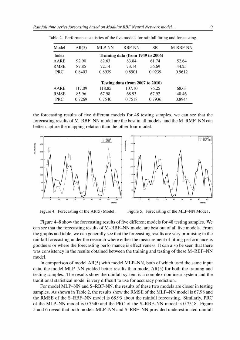
Testing data (from 2007 to 2010)AARE 117.09 118.85 107.10 76.25 68.63RMSE 85.96 67.98 68.93 67.92 48.46PRC 0.7269 0.7540 0.7518 0.7936 0.8944
the forecasting results of five different models for 48 testing samples, we can see that theforecasting results of M–RBF–NN model are the best in all models, and the M–RMF–NN canbetter capture the mapping relation than the other four model.
5 10 15 20 25 30 35 40 450
50
100
150
200
250
300
350
400
Month
Rai
nfa
ll(m
m)
ActualAR(5)
Figure 4. Forecasting of the AR(5) Model .
5 10 15 20 25 30 35 40 450
50
100
150
200
250
300
350
400
Month
Rai
nfal
l(mm
)
ActualMLP−NN
Figure 5. Forecasting of the MLP-NN Model .
Figure 4–8 show the forecasting results of five different models for 48 testing samples. Wecan see that the forecasting results of M–RBF–NN model are best out of all five models. Fromthe graphs and table, we can generally see that the forecasting results are very promising in therainfall forecasting under the research where either the measurement of fitting performance isgoodness or where the forecasting performance is effectiveness. It can also be seen that therewas consistency in the results obtained between the training and testing of these M–RBF–NNmodel.
In comparison of model AR(5) with model MLP–NN, both of which used the same inputdata, the model MLP–NN yielded better results than model AR(5) for both the training andtesting samples. The results show the rainfall system is a complex nonlinear system and thetraditional statistical model is very difficult to use for accuracy prediction.
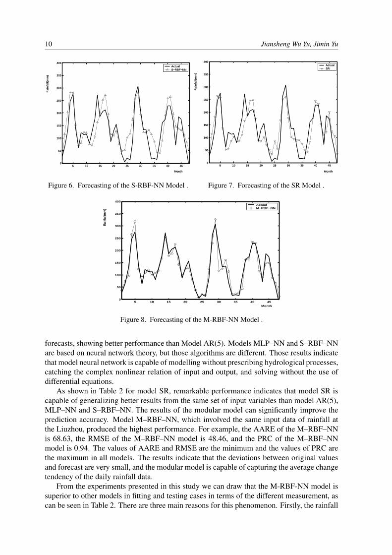
For model MLP–NN and S–RBF-NN, the results of these two models are closer in testingsamples. As shown in Table 2, the results show the RMSE of the MLP–NN model is 67.98 andthe RMSE of the S–RBF–NN model is 68.93 about the rainfall forecasting. Similarly, PRCof the MLP–NN model is 0.7540 and the PRC of the S–RBF–NN model is 0.7518. Figure5 and 6 reveal that both models MLP–NN and S–RBF–NN provided underestimated rainfall
10 Jiansheng Wu Yu, Jimin Yu
5 10 15 20 25 30 35 40 450
50
100
150
200
250
300
350
400
Month
Rai
nfal
l(mm
)
ActualS−RBF−NN
Figure 6. Forecasting of the S-RBF-NN Model .
5 10 15 20 25 30 35 40 450
50
100
150
200
250
300
350
400
Month
Rai
nfa
ll(m
m)
ActualSR
Figure 7. Forecasting of the SR Model .
5 10 15 20 25 30 35 40 450
50
100
150
200
250
300
350
400
Month
Rain
fall(
mm
)
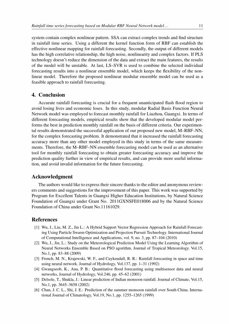
ActualM−RBF−NN
Figure 8. Forecasting of the M-RBF-NN Model .
forecasts, showing better performance than Model AR(5). Models MLP–NN and S–RBF–NNare based on neural network theory, but those algorithms are different. Those results indicatethat model neural network is capable of modelling without prescribing hydrological processes,catching the complex nonlinear relation of input and output, and solving without the use ofdifferential equations.
As shown in Table 2 for model SR, remarkable performance indicates that model SR iscapable of generalizing better results from the same set of input variables than model AR(5),MLP–NN and S–RBF–NN. The results of the modular model can significantly improve theprediction accuracy. Model M–RBF–NN, which involved the same input data of rainfall atthe Liuzhou, produced the highest performance. For example, the AARE of the M–RBF–NNis 68.63, the RMSE of the M–RBF–NN model is 48.46, and the PRC of the M–RBF–NNmodel is 0.94. The values of AARE and RMSE are the minimum and the values of PRC arethe maximum in all models. The results indicate that the deviations between original valuesand forecast are very small, and the modular model is capable of capturing the average changetendency of the daily rainfall data.
From the experiments presented in this study we can draw that the M-RBF-NN model issuperior to other models in fitting and testing cases in terms of the different measurement, ascan be seen in Table 2. There are three main reasons for this phenomenon. Firstly, the rainfall
Rainfall time series forecasting based on Modular RBF Neural Network model. . . 11
system contain complex nonlinear pattern. SSA can extract complex trends and find structurein rainfall time series. Using a different the kernel function form of RBF can establish theeffective nonlinear mapping for rainfall forecasting. Secondly, the output of different modelshas the high correlative relationship, the high noise, nonlinearity and complex factors. If PLStechnology doesn’t reduce the dimension of the data and extract the main features, the resultsof the model will be unstable. At last, LS–SVR is used to combine the selected individualforecasting results into a nonlinear ensemble model, which keeps the flexibility of the non-linear model. Therefore the proposed nonlinear modular ensemble model can be used as afeasible approach to rainfall forecasting.
4. ConclusionAccurate rainfall forecasting is crucial for a frequent unanticipated flash flood region to
avoid losing lives and economic loses. In this study, modular Radial Basis Function NeuralNetwork model was employed to forecast monthly rainfall for Liuzhou, Guangxi. In terms ofdifferent forecasting models, empirical results show that the developed modular model per-forms the best in prediction monthly rainfall on the basis of different criteria. Our experimen-tal results demonstrated the successful application of our proposed new model, M–RBF–NN,for the complex forecasting problem. It demonstrated that it increased the rainfall forecastingaccuracy more than any other model employed in this study in terms of the same measure-ments. Therefore, the M–RBF–NN ensemble forecasting model can be used as an alternativetool for monthly rainfall forecasting to obtain greater forecasting accuracy and improve theprediction quality further in view of empirical results, and can provide more useful informa-tion, and avoid invalid information for the future forecasting.
AcknowledgmentThe authors would like to express their sincere thanks to the editor and anonymous review-
ers comments and suggestions for the improvement of this paper. This work was supported byProgram for Excellent Talents in Guangxi Higher Education Institutions, by Natural ScienceFoundation of Guangxi under Grant No. 2011GXNSFE018006 and by the Natural ScienceFoundation of China under Grant No.11161029.
References[1] Wu, J., Liu, M. Z., Jin L.: A Hybrid Support Vector Regression Approach for Rainfall Forecast-
ing Using Particle Swarm Optimization and Projection Pursuit Technology. International Journalof Computational Intelligence and Applications, vol. 9, no. 3, pp. 87–104 (2010)
[2] Wu, J., Jin, L.: Study on the Meteorological Prediction Model Using the Learning Algorithm ofNeural Networks Ensemble Based on PSO agorithm. Journal of Tropical Meteorology. Vol.15,No.1, pp. 83–88 (2009)
[3] French, M. N., Krajewski, W. F., and Cuykendall, R. R.: Rainfall forecasting in space and timeusing neural network. Journal of Hydrology, Vol.137, pp. 1–31 (1992)
[4] Gwangseob, K., Ana, P. B.: Quantitative flood forecasting using multisensor data and neuralnetworks, Journal of Hydrology, Vol.246, pp. 45–62 (2001)
[5] Delsole, T., Shukla, J.: Linear prediction of Indian monsoon rainfall. Journal of Climate, Vol.15,No.1, pp. 3645–3658 (2002)
[6] Chan, J. C. L., Shi, J. E.: Prediction of the summer monsoon rainfall over South China. Interna-tional Journal of Climatology, Vol.19, No.1, pp. 1255–1265 (1999)

12 Jiansheng Wu Yu, Jimin Yu
[7] Wu, J.: A novel artificial neural network ensemble model based on K–nn nonparametric estima-tion of regression function and its application for rainfall forecasting. In Proeedings of the 2ndInternatioal Joint Conference on Computational Sciences and Optimization, eds. Lean Yu, K. K.Lai and S. K. Mishra, IEEE Computer Society Press, vol. 2, pp. 44–48, 2009.
[8] Wu, J.: A novel nonparametric regression ensemble for rainfall forecasting using particle swarmoptimization technique coupled with artificial neural network. Lecture Note in Computer Sci-ence, Vol. 5553, No. 3, pp. 49–58 (2009)
[9] Wu, J., Liu, M., Jin. L.: Least square support vector machine ensemble for daily rainfall forecast-ing bBased on linear and nonlinear rRegression. In: Zeng. Z., Wang. J.(eds.) Advance in NeuralNetwork Research & Application. LNEE, Vol. 67, pp. 55-64 (2010)
[10] Lin, G.F., Wu, M. C.: A hybrid neural network model for typhoon-rainfall forecasting. Journalof Hydrology, Vol. 375 (3–4), pp. 450-458 (2009)
[11] Banfield, R. E., Hall, L. O., Bowyer, K. W., Kegelmeyer, W. P.: Ensemble diversity measuresand their application to thinning. Information Fusion, Vol. 6, No. 1, pp. 49–62, (2005)
[12] Partalas, I., Hatzikos, E., Tsoumakas, G., Vlahavas, I.: Ensemble selection for water quality pre-diction. In Proeedings of 10th International Conference on Engineering Applications of NeuralNetworks, pp. 428–435 (2007)
[13] Broomhead, D. S., King, G. P.: Extracting Qualitative Dynamics from Experimental Data. Phys-ica D, Vol. 20, pp. 217–236 (1986)
[14] Alexandrov, T., Bianconcini, S., Dagum, E. B., Maass, P., McElroy, T. S.: A Review of SomeModern Approaches to The Problem of Trend Extraction. Technical report, US Census BureauRRS2008/03 (2008)
[15] No K. M., Singular Spectrum Analysis. Technical report, University of California (2009)[16] Golyandina, N., Nekrutkin, V., Zhigljavsky, A.: Analysis of Time Series Structure: SSA and
Related Techniques. Technical report, Chapman & Hall/crc (2001)[17] Wu, J., A Semi-parametric Regression Ensemble Model for Rainfall Forecasting Based on RBF
Neural Network, Lecture Notes in Artificial Intelligence and Computational Intelligence, Vol.6320, No.2, pp. 284–292 (2010).
[18] Moravej, Z., Vishwakarma, D. N., Singh, S. P.: Application of Radial Basis Function Neural Net-work for Differential Relaying of a Power Transformer, Computers and Electrical Engineering,Vol. 29, pp. 421–434 (2003)
[19] Ham, F. M., Kostanic, I.: Principles of Neurocomputing for Science & Engineering, theMcGraw-Hill Companies, New York (2001)
[20] Wold, S., Ruhe, A., Wold, H., Dunn, W. J.: The Collinearity Problem in Linear Regression:the Partial Least Squares Approach to Generalized Inverses. Journal on Scientific and StatisticalComputing, Vol. 5, No. 3, pp. 735–43 (1984)
[21] Pirouz, D. M.: An Overview of Partial Least Square. Technical report, The Paul Merage Schoolof Business, University of California, Irvine (2006)
[22] Suykens, J., Gestel, T., Van, J.: Least Squares Support Vector Machines, the World ScientificPublishing, Singapore (2002)
[23] Schokopf, B., Smola, A. J.: Learning with Kernels: Support Vector Machines, Regularization,Optimization, and Beyond. the MIT Press, Cambridge (2002)
[24] Wang, H., Li E., Li, G. Y., The Least Square Support Vector Regression Coupled with ParallelSampling Scheme Metamodeling Technique and Application in Sheet Forming Optimization.Materials and Design, Vol. 30, pp. 1468–1479 (2009)
[25] Yu, L.,Wang, S. Y., Lai, K. K.: A Novel Nonlinear Ensemble Forecasting Model IncorporatingGLAR and ANN for Foreign Exchange Rates. Computers & Operations Research, Vol. 32, pp.2523–2541 (2005)

Journal of Theoretical and Applied Computer Science Vol. 6, No. 2, 2012, pp. 13-26
ISSN 2299-2634 http://www.jtacs.org
Towards expert-based modelling of integrated software
quality
Łukasz Radliński
University of Szczecin, Faculty of Economics and Management
Abstract: This paper reports on a part of a project aimed at building an probabilistic model for inte-
grated software quality simulation and prediction. This paper discusses results of the ques-
tionnaire survey focused on gathering expert knowledge about the factors influencing vari-
ous features of software quality. Specifically, this analysis identifies project and process
factors of software quality, investigates relationships between quality features and their
sub-features as well as priorities for quality features. The survey has been performed
among software engineering experts and projects managers. Obtained results will be used
to calibrate that model for software quality simulation and prediction. These results also
partially deliver a general overview on how software quality features are perceived by in-
dustry.
Keywords: software quality, software process, expert knowledge, survey study, data analysis
1. Introduction
Quality is one of the main drivers in software projects. Achieving high level of software
quality is difficult without appropriate management activities that require certain inputs.
These inputs may have various sources, such as expert judgment, process data or software
metrics. They may be combined in models to enable reuse of existing knowledge in differ-
ent projects. Such models can be used for estimation, simulation and prediction of software
quality and thus extend the base for decision support.
Quality prediction models have been built since the turn of 1960’s and 1970’s. They in-
volved using a range of techniques such as regression, neural networks, decision trees, sup-
port vector machines, case-based reasoning [17]. A common feature of these models is that
they are typically focused on a single attribute of quality, such as number of defects, defect-
proneness, reliability, security, usability, maintainability, etc. [6][7][8]. Very few models
incorporate multiple software quality features.
The aim of an on-going research project is to develop a model that could be used for
simulation and prediction of integrated software quality. In this context the term ‘integra-
tion’ refers to capturing a variety of quality features, linked with each other and with a set of
influential factors, in a single model. Earlier analyses of empirical data and attempts to build
a simulation and predictive model have been published in [10][11][13][14].
The aim of this paper is to analyze the results of surveys that have been performed
among experienced project managers and software engineering experts. The goal of these
surveys was to gather opinions on factors that influence different quality features. The re-
sults of this analysis serve as one of the sources for developed simulation model.

14 Łukasz Radliński
The paper is organized as follows: Section 2 discusses the background and motivation
for this study. Section 3 considers the research approach by explaining the procedure, sum-
mary of techniques used and the questionnaire design. Section 4 provides the details of the
results of the analysis. Section 5 discusses lessons learned and threats to validity of achieved
results. Section 6 provides conclusions and ideas for future work.
2. Background and motivation
The aim of the surveys among software engineering experts and project managers was to
gather personal knowledge on the factors influencing quality features. These surveys have
been performed to calibrate a Bayesian network model for software quality prediction and
simulation. The core structure of that model has been defined in advance. Figure 1 illus-
trates the schematic of this model. The model has a modular structure, i.e., variables are
grouped into topical subnets:
• Project factors – contains various factors describing the nature of the project and its
environment, i.e. architecture, CASE tool usage, deployment platform, user interface
type, target market, used methodology, project difficulty. These project factors influ-
ence selected quality features.
• Process factors – contains various factors describing the quality of development pro-
cess. Depending on particular version of the model, this subnet may be more or less
complex. In the smallest version it contains only very few details – effort and overall
process quality, separately for each of three main development activities: specifica-
tion, development and testing. In the most complex version it contains detailed pro-
cess and people factors as discussed in Section 4.5 and illustrated in Figure 6. These
process factors influence selected quality features.
• Quality features – contains a set of interconnected high-level features reflecting
software quality.
• Quality features, sub-features and measures – contains a hierarchy of software quali-
ty where features are decomposed into a set of sub-features, and sub-features may
have detailed quantitative measures assigned. This hierarchy is based on an ISO
25010 standard [1].
• Integration of components – enables reflecting integration of software components
into larger artifacts such as sub-systems and systems and thus modeling the level of
aggregated quality features.
It is beyond the scope of this paper to discuss the details of this model. Interested readers
may find the details in [10][11][13].
The motivation for developing this model is the fact that we have not found another
model aimed at predicting/simulating such variety of factors. Typically existing models are
focused on a single feature of quality, such as maintainability [15] or defects [1][3][4]. After
extensive literature survey we found only two studies closely relevant to the one that we
have been developing.
The first of them [2], explicitly refers to the ISO 9126 standard, the predecessor of ISO
25010 standard that we have been using. However, there are two main problems with pro-
posed model. The author does not provide details on the quantitative definition of that mod-
el, i.e. probability distributions. Thus, it is difficult to validate and reuse that model. Addi-
tionally, it was developed based on the data from small student projects. Therefore, it may
be out of scope for larger industry-scale projects.

Towards expert-based modelling of integrated software quality 15
Software
Sub-system
Software Component 2
Software Component 1
Project
Factors
Process
Factors
Quality
Features
Sub-features
Measures
Quality
Features
Project
Factors
Process
Factors
Quality
Features
Sub-features
Measures
Quality
Features
Quality
Features
Figure 1. Schematic of the Integrated Model for Software Quality Prediction
The second study [16] was focused on developing a framework for building Bayesian
networks for software quality prediction. However, it is not clear if a proposed framework
can be effectively used to build models for integrated software quality prediction, i.e. where
quality features depend on other factors but also on each other, as is the case in our study.
3. Research approach
3.1. Research procedure
As mentioned earlier, the questionnaire survey is a part of a larger work aimed at devel-
oping an integrated model for software quality prediction and simulation. The main stages
of this work involve the following steps:
1. Defining the core structure of the model – results published in [10][11][13].
2. Gathering empirical data to partially calibrate the model – partial results published in
[12][14].
3. Gathering subjective expert knowledge to partially calibrate the model – this is the
core of this study.
4. Calibrating the model using a combination of results from steps 2 and 3 – future
work.
5. Validating the model – future work.
To gather subjective expert knowledge we performed a questionnaire survey among
software engineering experts and project/team managers in software projects. The surveys
have been performed as direct interviews. We choose not to perform such survey by asking
respondents to fill out questionnaire on-line for two main reasons. First, when performing a
survey to calibrate an earlier model, we observed that some respondents provided responses
without sufficient focus and understanding of questions and answers. Second, although the

16 Łukasz Radliński
core questionnaire was a formalized document we wanted respondents to give an ability to
verbally provide additional information that was impossible to be included in the question-
naire. To support this, some interviews were recorded and during other we were taking live
notes.
During the interview we presented five different versions of the model for integrated
software quality prediction. The differences between models were related to the level of de-
tails of particular sub-networks. The aim of this step was to briefly familiarize respondents
with the objective and the background of the interview. Then, during the main part of the
interview we asked respondents to fill our questionnaire forms, one-by-one. The average
duration of an interview was about 1:55 hours, the shortest took 1:25 hours and the longest
2:17 hours. The details of this questionnaire forms are discussed in Section 3.2.
We performed the interviews with eight selected respondents from six companies, of
which four are Polish branches of major international IT companies, one an IT department
of a large Polish bank, and one a systems development department of major electronics sup-
plier for automotive industry based in Germany. The subjects for these interviews were se-
lected based on their knowledge and experience in software development, in particular in
software quality. Some of them participated in earlier studies on software validation and
verification or calibration of earlier Bayesian network models.
After performing the interviews, we aggregated gathered data and performed cleaning.
At this stage we corrected obvious mistakes that even some respondents noticed during an
interview, for example the direction of the influence of particular factor on another one.
Then we performed data analysis that involved variety of analytical techniques, such as
basic measures of central tendency and variability, Spearman’s rank correlation coefficient
[9]. In addition, the analysis involved visual techniques, such as histograms, box-plots, scat-
ter-plots as well as other custom graphs. The results of these analyses will serve as the input
to the developed simulation model formally represented as a Bayesian network.
3.2. Questionnaire design
The main part of the questionnaire consists of seven groups of questions:
1. Importance of quality features – reflecting respondent’s opinion on the priority for
each quality feature expressed on a scale [0, 10].
2. Relationships between quality features – reflecting respondent’s opinion on how
strong are quality features related with each other. The lowest value ‘-5’ indicates
strong negative relationship, the value ‘0’ – no relationship, and the highest value
‘+5’ – strong positive relationship.
3. Hierarchy of quality features – reflecting respondent’s opinion on the strength of re-
lationships between each feature and a set of its individual sub-features. The same
scale as in point 2.
4. Strength of impact of development process on quality features – reflecting respond-
ent’s opinion on how each of the main processes, i.e. specification, development and
testing, influences quality features. The same scale as in point 2.
5. Relationships among detailed process factors – reflecting respondent’s opinion on
the factors that influence the aggregated process quality, separately for specification,
development and testing. The same scale as in point 2.
6. Impact of project factors on quality features – reflecting respondent’s opinion on the
presence (indicated by entering a ‘+’ sign) or absence (a ‘–‘ sign) of the impact of
seven predefined project factors on quality features.
Towards expert-based modelling of integrated software quality 17
7. Strength of impact of project factors on quality features – reflecting respondent’s
opinion on the strength of impact of seven predefined project factors on quality fea-
tures. This is an extension of point 6. The strength is expressed also on a scale
[-5, 5]. But here the scale has a different interpretation. A value ‘-5’ indicates that
with a presence of specific project factor a given quality feature is expected to have a
very low level. A value ‘+5’ indicates that with a presence of specific project factor
a given quality feature is expected to have a very high level.
Respondents were asked to provide answers as integer numbers. However, they were al-
so informed that they may provide answers as intermediate values, e.g. ‘3.5’, or as ranges,
e.g. [2-3] or [-2, 3].
4. Results
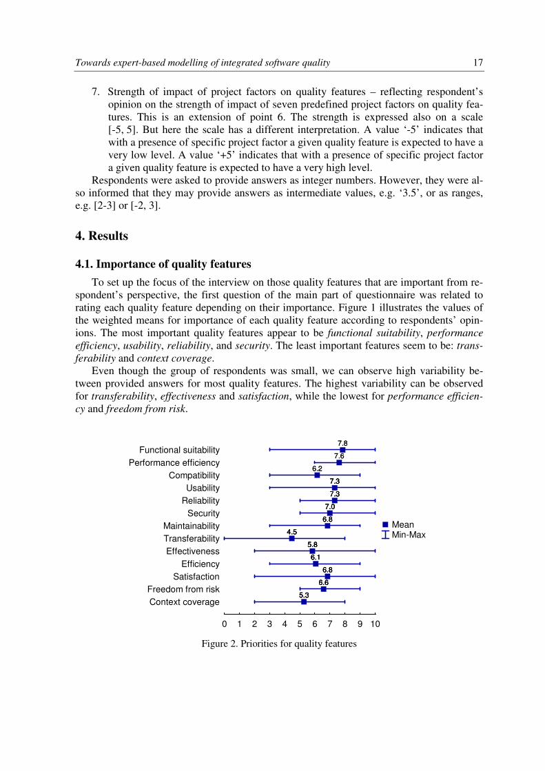
4.1. Importance of quality features
To set up the focus of the interview on those quality features that are important from re-
spondent’s perspective, the first question of the main part of questionnaire was related to
rating each quality feature depending on their importance. Figure 1 illustrates the values of
the weighted means for importance of each quality feature according to respondents’ opin-
ions. The most important quality features appear to be functional suitability, performance
efficiency, usability, reliability, and security. The least important features seem to be: trans-
ferability and context coverage.
Even though the group of respondents was small, we can observe high variability be-
tween provided answers for most quality features. The highest variability can be observed
for transferability, effectiveness and satisfaction, while the lowest for performance efficien-
cy and freedom from risk.
Mean Min-Max
5.3
6.6
6.8
6.1
5.8
4.5
6.8
7.0
7.3
7.3
6.2
7.6
7.8
5.3
6.6
6.8
6.1
5.8
4.5
6.8
7.0
7.3
7.3
6.2
7.6
7.8
0 1 2 3 4 5 6 7 8 9 10
Context coverage
Freedom from risk
Satisfaction
Efficiency
Effectiveness
Transferability
Maintainability
Security
Reliability
Usability
Compatibility
Performance efficiency
Functional suitability
5.3
6.6
6.8
6.1
5.8
4.5
6.8
7.0
7.3
7.3
Figure 2. Priorities for quality features
18 Łukasz Radliński
Quality features
Functional
suitabili
ty
Perf
orm
ance
eff
icie
ncy
Com
patibili
ty
Usabili
ty
Relia
bili
ty
Security
Main
tain
abili
ty
Tra
nsfe
rabili
ty
Eff
ectiveness
Effic
iency
Satisfa
ction
Fre
edom
fr
om
ris
k
Conte
xt
covera
ge
Functional suitability
0.48 0.47
Performance efficiency
0.77
0.68
-0.70 0.74
Compatibility
-0.79
-0.66
-0.81 -0.79 -0.55
Usability
-0.79
0.51
-0.72 0.94 0.92 0.71 -0.51 0.48
Reliability
0.77
0.81
Security 0.48
-0.66 0.51
-0.58
0.59
Maintainability 0.47 0.68
-0.55
Transferability
-0.72
-0.58
-0.61 -0.83
-0.68
Effectiveness
-0.81 0.94
-0.55 -0.61
0.90 0.71
Efficiency
-0.79 0.92
0.59
-0.83 0.90
0.66
0.51
Satisfaction
-0.70 -0.55 0.71
0.71 0.66
0.50
Freedom from risk
0.74
-0.51 0.81
-0.64
Context coverage
0.48
-0.68
0.51 0.50 -0.64
Figure 3. Spearman’ correlations between priorities of quality features
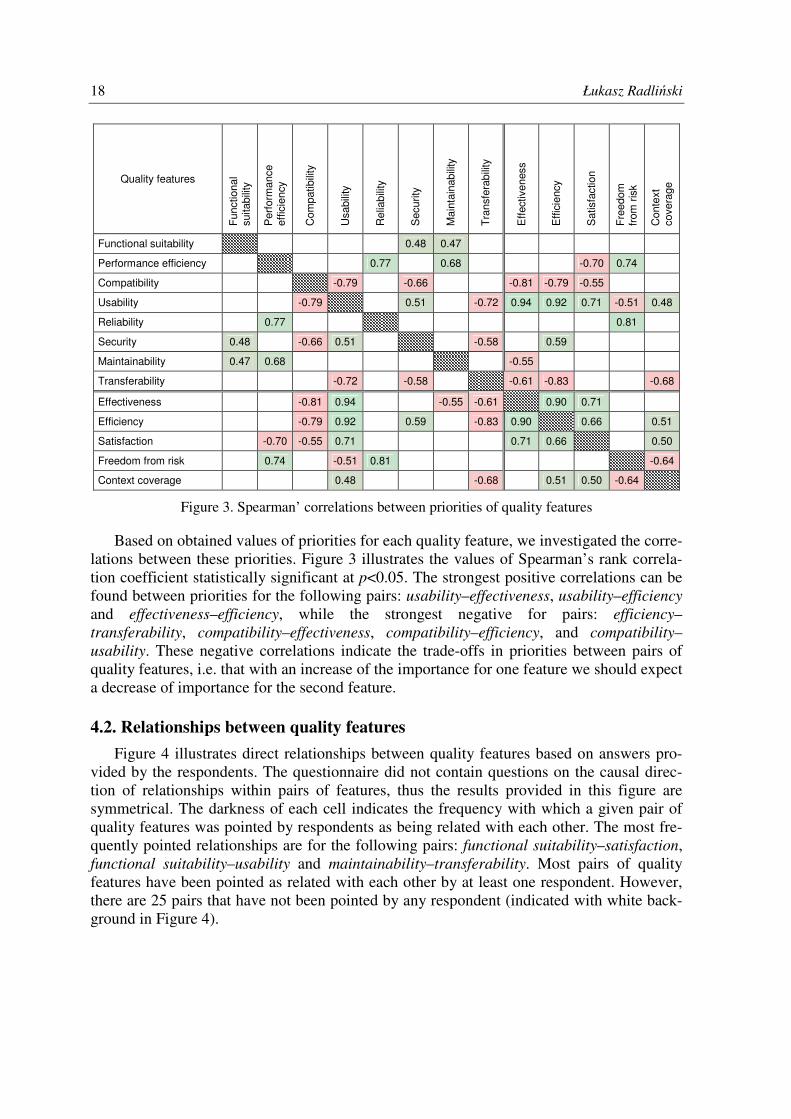
Based on obtained values of priorities for each quality feature, we investigated the corre-
lations between these priorities. Figure 3 illustrates the values of Spearman’s rank correla-
tion coefficient statistically significant at p<0.05. The strongest positive correlations can be
found between priorities for the following pairs: usability–effectiveness, usability–efficiency
and effectiveness–efficiency, while the strongest negative for pairs: efficiency–
transferability, compatibility–effectiveness, compatibility–efficiency, and compatibility–
usability. These negative correlations indicate the trade-offs in priorities between pairs of
quality features, i.e. that with an increase of the importance for one feature we should expect
a decrease of importance for the second feature.
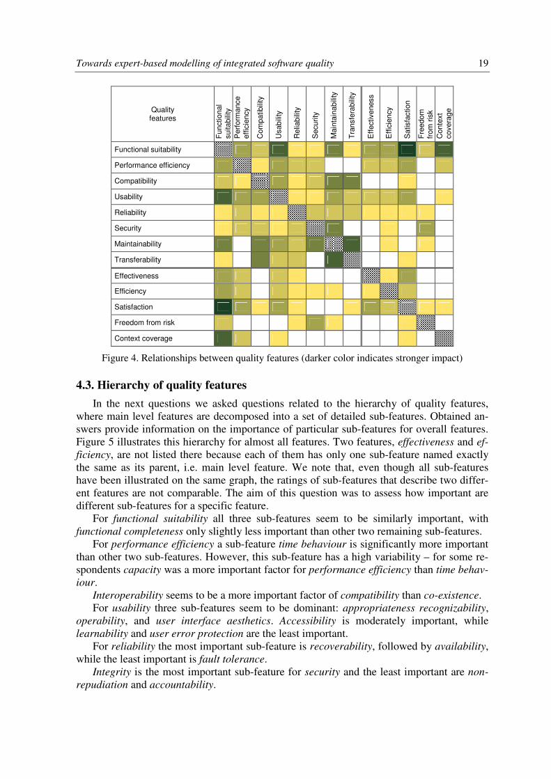
4.2. Relationships between quality features
Figure 4 illustrates direct relationships between quality features based on answers pro-
vided by the respondents. The questionnaire did not contain questions on the causal direc-
tion of relationships within pairs of features, thus the results provided in this figure are
symmetrical. The darkness of each cell indicates the frequency with which a given pair of
quality features was pointed by respondents as being related with each other. The most fre-
quently pointed relationships are for the following pairs: functional suitability–satisfaction,
functional suitability–usability and maintainability–transferability. Most pairs of quality
features have been pointed as related with each other by at least one respondent. However,
there are 25 pairs that have not been pointed by any respondent (indicated with white back-
ground in Figure 4).
Towards expert-based modelling of integrated software quality 19
Quality features
Functional
suitabili
ty
Perf
orm
ance
eff
icie
ncy
Com
patibili
ty
Usabili
ty
Relia
bili
ty
Security
Main
tain
abili
ty
Tra
nsfe
rabili
ty
Eff
ectiveness
Effic
iency
Satisfa
ction
Fre
edom
fr
om
ris
k
Conte
xt
covera
ge
Functional suitability
Performance efficiency
Compatibility
Usability
Reliability
Security
Maintainability
Transferability
Effectiveness
Efficiency
Satisfaction
Freedom from risk
Context coverage
Figure 4. Relationships between quality features (darker color indicates stronger impact)
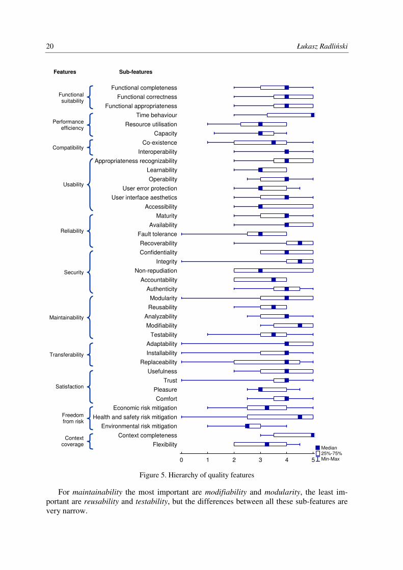
4.3. Hierarchy of quality features
In the next questions we asked questions related to the hierarchy of quality features,
where main level features are decomposed into a set of detailed sub-features. Obtained an-
swers provide information on the importance of particular sub-features for overall features.
Figure 5 illustrates this hierarchy for almost all features. Two features, effectiveness and ef-
ficiency, are not listed there because each of them has only one sub-feature named exactly
the same as its parent, i.e. main level feature. We note that, even though all sub-features
have been illustrated on the same graph, the ratings of sub-features that describe two differ-
ent features are not comparable. The aim of this question was to assess how important are
different sub-features for a specific feature.
For functional suitability all three sub-features seem to be similarly important, with
functional completeness only slightly less important than other two remaining sub-features.
For performance efficiency a sub-feature time behaviour is significantly more important
than other two sub-features. However, this sub-feature has a high variability – for some re-
spondents capacity was a more important factor for performance efficiency than time behav-
iour.
Interoperability seems to be a more important factor of compatibility than co-existence.
For usability three sub-features seem to be dominant: appropriateness recognizability,
operability, and user interface aesthetics. Accessibility is moderately important, while
learnability and user error protection are the least important.
For reliability the most important sub-feature is recoverability, followed by availability,
while the least important is fault tolerance.
Integrity is the most important sub-feature for security and the least important are non-
repudiation and accountability.
20 Łukasz Radliński
Figure 5. Hierarchy of quality features
For maintainability the most important are modifiability and modularity, the least im-
portant are reusability and testability, but the differences between all these sub-features are
very narrow.
Median 25%-75% Min-Max 0 1 2 3 4 5
Flexibility
Context completeness
Environmental risk mitigation
Health and safety risk mitigation
Economic risk mitigation
Comfort
Pleasure
Trust
Usefulness
Replaceability
Installability
Adaptability
Testability
Modifiability
Analyzability
Reusability
Modularity
Authenticity
Accountability
Non-repudiation
Integrity
Confidentiality
Recoverability
Fault tolerance
Availability
Maturity
Accessibility
User interface aesthetics
User error protection
Operability
Learnability
Appropriateness recognizability
Interoperability
Co-existence
Capacity
Resource utilisation
Time behaviour
Functional appropriateness
Functional correctness
Functional completenessFunctionalsuitability
Performance efficiency
Compatibility
Usability
Reliability
Security
Maintainability
Transferability
Satisfaction
Freedomfrom risk
Contextcoverage
Features Sub-features
Towards expert-based modelling of integrated software quality 21
For transferability all three its sub-features are on the similar level. Interestingly, all
three sub-features have very high variability and cover the whole range [0, 5] of possible
values.
Usefulness seems to be the most important factor for satisfaction, and pleasure the least
important.
For freedom from risk the most important seems to be health and safety risk mitigation
and the least important – environmental risk mitigation.
For context coverage a sub-feature context completeness seems to be significantly more
important than flexibility.
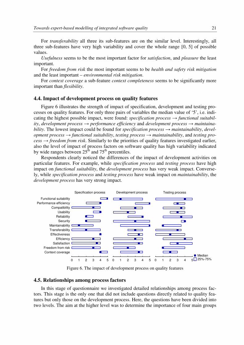
4.4. Impact of development process on quality features
Figure 6 illustrates the strength of impact of specification, development and testing pro-
cesses on quality features. For only three pairs of variables the median value of ‘5’, i.e. indi-
cating the highest possible impact, were found: specification process → functional suitabil-
ity, development process → performance efficiency and development process → maintaina-
bility. The lowest impact could be found for specification process → maintainability, devel-
opment process → functional suitability, testing process → maintainability, and testing pro-
cess → freedom from risk. Similarly to the priorities of quality features investigated earlier,
also the level of impact of process factors on software quality has high variability indicated
by wide ranges between 25th
and 75th
percentiles.
Respondents clearly noticed the differences of the impact of development activities on
particular features. For example, while specification process and testing process have high
impact on functional suitability, the development process has very weak impact. Converse-
ly, while specification process and testing process have weak impact on maintainability, the
development process has very strong impact.
Specification process
0 1 2 3 4 5
Context coverage
Freedom from risk
Satisfaction
Efficiency
Effectiveness
Transferability
Maintainability
Security
Reliability
Usability
Compatibility
Performance efficiency
Functional suitability
Development process
0 1 2 3 4 5
Testing process
Median 25%-75% 0 1 2 3 4 5
Figure 6. The impact of development process on quality features
4.5. Relationships among process factors
In this stage of questionnaire we investigated detailed relationships among process fac-
tors. This stage is the only one that did not include questions directly related to quality fea-
tures but only those on the development process. Here, the questions have been divided into
two levels. The aim at the higher level was to determine the importance of four main groups
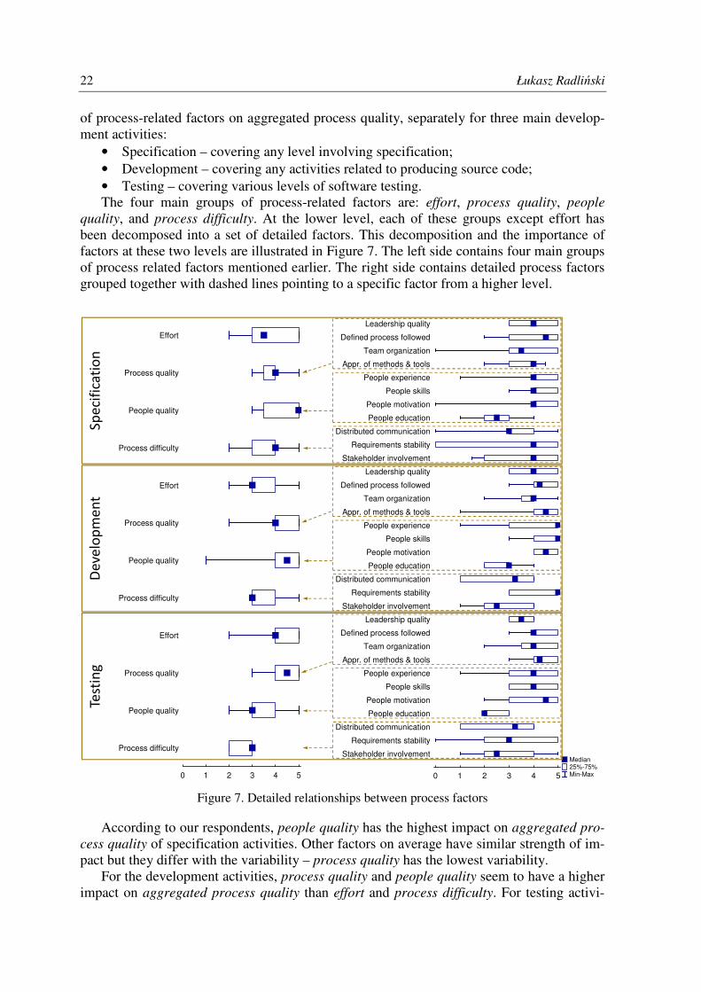
22 Łukasz Radliński
of process-related factors on aggregated process quality, separately for three main develop-
ment activities:
• Specification – covering any level involving specification;
• Development – covering any activities related to producing source code;
• Testing – covering various levels of software testing.
The four main groups of process-related factors are: effort, process quality, people
quality, and process difficulty. At the lower level, each of these groups except effort has
been decomposed into a set of detailed factors. This decomposition and the importance of
factors at these two levels are illustrated in Figure 7. The left side contains four main groups
of process related factors mentioned earlier. The right side contains detailed process factors
grouped together with dashed lines pointing to a specific factor from a higher level.
Median 25%-75% Min-Max 0 1 2 3 4 5
Stakeholder involvement
Requirements stability
Distributed communication
People education
People motivation
People skills
People experience
Appr. of methods & tools
Team organization
Defined process followed
Leadership quality
Stakeholder involvement
Requirements stability
Distributed communication
People education
People motivation
People skills
People experience
Appr. of methods & tools
Team organization
Defined process followed
Leadership quality
Stakeholder involvement
Requirements stability
Distributed communication
People education
People motivation
People skills
People experience
Appr. of methods & tools
Team organization
Defined process followed
Leadership quality
0 1 2 3 4 5
Process difficulty
People quality
Process quality
Effort
Process difficulty
People quality
Process quality
Effort
Process difficulty
People quality
Process quality
Effort
Specification
Development
Testing
Figure 7. Detailed relationships between process factors
According to our respondents, people quality has the highest impact on aggregated pro-
cess quality of specification activities. Other factors on average have similar strength of im-
pact but they differ with the variability – process quality has the lowest variability.
For the development activities, process quality and people quality seem to have a higher
impact on aggregated process quality than effort and process difficulty. For testing activi-
Towards expert-based modelling of integrated software quality 23
ties, the differences between factors are varying the most. Process quality and effort seem to
be the most important, people quality with the moderate impact, and process difficulty with
the least impact.
On the lower level (right side of Figure 7) we can also observe some differences in im-
portance of factors depending on development activities. For example, the impact of de-
tailed factors for process difficulty is varying strongly for specification activities and slightly
less for testing. However, for development activities the impact of these factors seem to be
more polarized – requirements stability significantly more important for process difficulty
than stakeholder involvement and distributed communication.
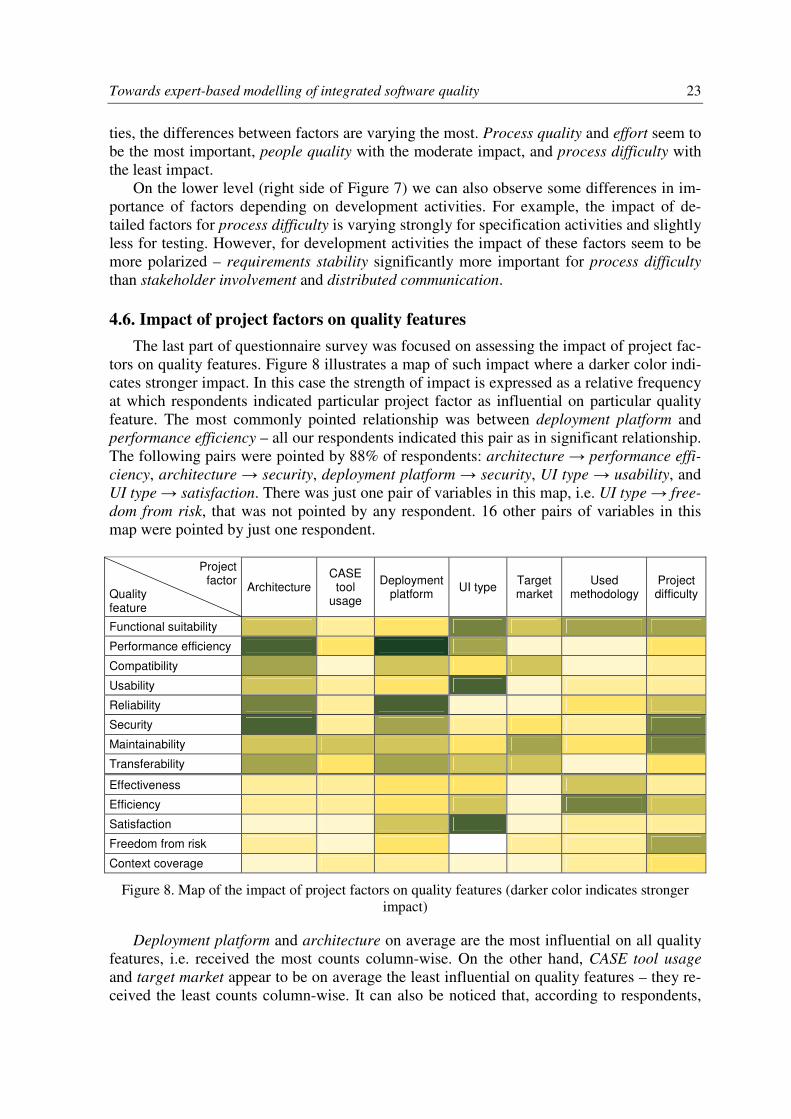
4.6. Impact of project factors on quality features
The last part of questionnaire survey was focused on assessing the impact of project fac-
tors on quality features. Figure 8 illustrates a map of such impact where a darker color indi-
cates stronger impact. In this case the strength of impact is expressed as a relative frequency
at which respondents indicated particular project factor as influential on particular quality
feature. The most commonly pointed relationship was between deployment platform and
performance efficiency – all our respondents indicated this pair as in significant relationship.
The following pairs were pointed by 88% of respondents: architecture → performance effi-
ciency, architecture → security, deployment platform → security, UI type → usability, and
UI type → satisfaction. There was just one pair of variables in this map, i.e. UI type → free-
dom from risk, that was not pointed by any respondent. 16 other pairs of variables in this
map were pointed by just one respondent.
Project
factor Quality feature
Architecture CASE
tool usage
Deployment platform
UI type Target market
Used methodology
Project difficulty
Functional suitability
Performance efficiency
Compatibility
Usability
Reliability
Security
Maintainability
Transferability
Effectiveness
Efficiency
Satisfaction
Freedom from risk
Context coverage
Figure 8. Map of the impact of project factors on quality features (darker color indicates stronger
impact)
Deployment platform and architecture on average are the most influential on all quality
features, i.e. received the most counts column-wise. On the other hand, CASE tool usage
and target market appear to be on average the least influential on quality features – they re-
ceived the least counts column-wise. It can also be noticed that, according to respondents,
24 Łukasz Radliński
these project factors have much weaker impact on the quality-in-use features – the last five
rows in Figure 8 are on average with much lighter shade than remaining top eight rows.
The questionnaire contained questions about the strength of impact of particular values
of project factors on quality features. Respondents were able either to use predefined values,
for example ‘standalone’, ‘client-server’ or ‘multi-tier’ for architecture or provide use their
own values. Because several respondents chose to use their own classification for these pro-
ject factors, obtained results cannot be easily aggregated. Such custom classifications were
typically used by single respondents.
5. Lessons learned and threats to validity
One of the main problems in this study is the low number of respondents. Thus, it is dif-
ficult to use more advanced quantitative analytical techniques that require more cases at in-
put. In addition, respondents represented diverse organizations, i.e. developing different
types of software and using different processes. However, we also note that the primary goal
of this survey was not to gather extensive knowledge on a wide range of projects and soft-
ware organizations. Instead, we were looking to analyze the variability of answers provided
by various experts.
Furthermore, the questionnaire contained questions aimed at calibrating a specific
Bayesian network model. Thus, the answers provided by our respondents may be biased and
would have been different for a model with another scope and structure.
The group of respondents was not homogeneous in terms of their background, age and
experience. For example, some respondents consider themselves more as managers than
software engineers. We also observed differences in respondents’ attitude to this survey.
Typically, those who were more strongly interested with potential usage of such model for
predictions and simulations, were also more focused on providing carefully considered an-
swers.
We informed respondents that, although the questionnaire has a structured form, re-
spondents may put additional notes or provide explanations verbally. Some respondents
used it to provide information on additional elements such as:
• Process activities – i.e. apart from specification, development and testing;
• Detailed process factors – typically related to process and people quality;
• Project factors – especially w the factors provided in the questionnaire were not rele-
vant to the nature of projects developed in their organizations.
Usually respondents provided answers inconsistent with other respondents. The differ-
ences covered not only the strength of relationships between investigated factors but also the
existence of relationship between certain pairs of factors. This exposed the general problem
of acquiring subjective knowledge and aggregating the results. The sources of these differ-
ences partially can be explained by the fact that respondents participate in developing di-
verse software projects in different software organizations. Therefore, it may not be sensible
to build a single simulation and predictive model but rather more tailored models for differ-
ent types of projects or organizations.
6. Conclusions and future work
The analysis performed in this study lead to the following conclusions:
1. There is a demand in industry to develop predictive and simulation models covering
a wider range of quality features. However, there are organizations and projects
where such models are not relevant and useful.
Towards expert-based modelling of integrated software quality 25
2. When assessing strength of impact of particular factors on quality features, most ex-
perts used a predefined set of factors, although they were able to provide other fac-
tors according to their point of view. Together with the fact that these relationships
were often seen as moderate, strong or very strong, this ensures us that the factors
that will be used in the model have been selected appropriately.
3. There is a high variability in experts’ perception on the factors that influence soft-
ware quality. While some experts may consider a particular factor as important for a
given quality feature, other experts may see such factors as not very important or
even further – as influencing with an opposite direction. Thus, it may be very diffi-
cult to aggregate these results into a single simulation and predictive model.
Overall, we believe that results discussed in this paper and the model may provide useful
support to decision makers in software projects. In future, we plan to extend this research by
combining these results from survey among software experts with more objective empirical
data, as well as to perform more detailed validation of the simulation model. Due to a high
variability of responses we also plan to investigate the possibility of developing models tai-
lored to individual needs and then to evaluate the usefulness of such models.
Acknowledgement
I would like to thank all participants of the questionnaire survey for providing useful in-
formation and additional thoughts inspiring this and further research. This work has been
supported by research funds from the Ministry of Science and Higher Education and the Na-
tional Science Centre in Poland as a research grant no. N N111 291738 for years 2010-2012.
References
[1] Abouelela M., Benedicenti L., Bayesian Network Based XP Process Modelling, Inter-
national Journal of Software Engineering and Applications, vol 1, no.3, pp. 1-15, 2010.
[2] Beaver J.M., A life cycle software quality model using Bayesian belief networks, Doc-
toral Dissertation, University of Central Florida, Orlando, FL, 2006.
[3] Fenton N., Hearty P., Neil M., Radliński Ł., Software Project and Quality Modelling
Using Bayesian Networks. In: Meziane, F., Vadera, S. (eds.) Artificial Intelligence Ap-
plications for Improved Software Engineering Development: New Prospects, Infor-
mation Science Reference, New York, pp. 1-25, 2008.
[4] Fenton N., Neil M., Marsh W., Hearty P., Radliński Ł., Krause P., On the effectiveness
of early life cycle defect prediction with Bayesian Nets, Empirical Software Engineer-
ing, vol. 13, pp. 499-537, 2008.
[5] ISO/IEC 25010:2011(E), Software engineering – Software product Quality Require-
ments and Evaluation (SQuaRE) – System and software quality models, 2011.
[6] Jones C., Applied Software Measurement: Global Analysis of Productivity and Quality,
Third Edition, McGraw-Hill, New York, 2008.
[7] Kan S. H., Metrics and Models in Software Quality Engineering, Addison-Wesley,
Boston, 2003.
[8] Lyu M., Handbook of software reliability engineering, McGraw-Hill, Hightstown, NJ,
1996.
[9] Maxwell, K.D.: Applied Statistics for Software Managers. Prentice Hall PTR, Upper
Saddle River, 2002.
[10] Radliński Ł., A conceptual Bayesian net model for integrated software quality predic-
tion, Annales UMCS, Informatica, vol. 11, no. 4, pp. 49-60, 2011.
26 Łukasz Radliński
[11] Radliński Ł., A Framework for Integrated Software Quality Prediction using Bayesian
Nets, in Proceedings of International Conference on Computational Science and Its
Applications (ICCSA 2011), Santander: Springer, 2011.
[12] Radliński Ł., Empirical Analysis of the Impact of Requirements Engineering on Soft-
ware Quality, Requirements Engineering: Foundation for Software Quality, Lecture
Notes in Computer Science, vol. 7195, Springer, Berlin-Heidelberg, pp. 232-238, 2012.
[13] Radliński Ł., Enhancing Bayesian Network Model for Integrated Software Quality
Prediction, in Proc. Fourth International Conference on Information, Process, and
Knowledge Management, Valencia, 2012, pp. 144-149.
[14] Radliński Ł., Factors of Software Quality – Analysis of Extended ISBSG Dataset,
Foundations of Computing and Decision Studies, vol. 36, no. 3-4, pp. 293-313, 2011.
[15] Van Koten C., Gray A.R., An application of Bayesian network for predicting object-
oriented software maintainability, Information and Software Technology, vol. 48,
pp. 59-67, 2006.
[16] Wagner S., A Bayesian network approach to assess and predict software quality using
activity-based quality models, In: 5th Int. Conf. on Predictor Models in Software Engi-
neering, ACM Press, New York, 2009.
[17] Zhang D., Tsai J. J. P., Machine Learning and Software Engineering, Software Quality
Journal, vol. 11, no. 2, pp. 87-119, 2003.
Journal of Theoretical and Applied Computer Science Vol. 6, No. 2, 2012, pp. 27–44ISSN 2299-2634 http://www.jtacs.org
Is the conventional interval arithmetic correct?
Andrzej PiegatFaculty of Computer Science, West Pomeranian University of Technology, Szczecin, [email protected]
Marek LandowskiInstitute of Quantitative Methods, Maritime University of Szczecin, [email protected]
Abstract: Interval arithmetic as part of interval mathematics and Granular Computing is unusually im-portant for development of science and engineering in connection with necessity of taking intoaccount uncertainty and approximativeness of data occurring in almost all calculations. Intervalarithmetic also conditions development of Artificial Intelligence and especially of automatic think-ing, Computing with Words, grey systems, fuzzy arithmetic and probabilistic arithmetic. However,the mostly used conventional Moore-arithmetic has evident weak-points. These weak-points arewell known, but nonetheless it is further on frequently used. The paper presents basic operations ofRDM-arithmetic that does not possess faults of Moore-arithmetic. The RDM-arithmetic is basedon multi-dimensional approach, the Moore-arithmetic on one-dimensional approach to intervalcalculations. The paper also presents a testing method, which allows for clear checking whetherresults of any interval arithmetic are correct or not. The paper contains many examples andillustrations for better understanding of the RDM-arithmetic. In the paper, because of volumelimitations only operations of addition and subtraction are discussed. Operations of multiplica-tion and division of intervals will be presented in next publication. Author of the RDM-arithmeticconcept is Andrzej Piegat.
Keywords: interval arithmetic, RDM-interval arithmetic, multi-dimensional interval arithmetic, intervalmathematics, interval analysis, granular computing, artificial intelligence
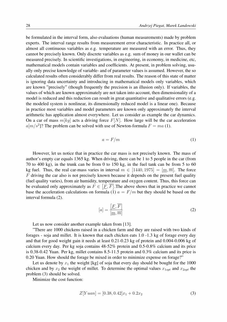
1. IntroductionInterval arithmetic comprises basic operations as addition, subtraction, multiplication and
division of intervals. With its use one can e.g. add two quantities a and b, values of which arenot precisely but only approximatively known and the approximation has form of interval, e.g.a ∈ [1, 3] and b ∈ [3, 5]. Interval arithmetic seems to be a less important area of mathematicsand many students, engineers and scientists do not use it or even do not know about its exis-tence. Meanwhile, the interval arithmetic has become a very important branch of mathematicsin consequence of realization by many engineers and scientists of the fact that for achievingmore credible problem solutions one should use any available information piece about a prob-lem. Not only numerical and precise but also all approximate data pieces should be used. Thisaim was formulated e.g. for the famous and rapidly developing Grey Systems Theory [8] byits creator Professor Yulong Deng, a theory that undoubtedly can be called ”mathematics ofthe future”. Similar aims has Granular Computing [11]. Interval approximations probably areapproximation forms the most frequently used in practice. Any technical measurement can
28 Andrzej Piegat, Marek Landowski
be formulated in the interval form, also evaluations (human measurements) made by problemexperts. The interval range results from measurement error characteristic. In practice all, oralmost all continuous variables as e.g. temperature are measured with an error. Thus, theycannot be precisely known. Only discrete variables as e.g. sum of money in our wallet can bemeasured precisely. In scientific investigations, in engineering, in economy, in medicine, etc,mathematical models contain variables and coefficients. At present, in problem solving, usu-ally only precise knowledge of variable- and of parameter values is assumed. However, the socalculated results often considerably differ from real results. The reason of this state of matteris ignoring data uncertainty and introducing in mathematical models only variables, whichare known ”precisely” (though frequently the precision is an illusion only). If variables, thevalues of which are known approximately are not taken into account, then dimensionality of amodel is reduced and this reduction can result in great quantitative and qualitative errors (e.g.the modeled system is nonlinear, its dimensionally reduced model is a linear one). Becausein practice most variables and model parameters are known only approximately the intervalarithmetic has application almost everywhere. Let us consider as example the car dynamics.On a car of mass m[kg] acts a driving force F [N ]. How large will be the car accelerationa[m/s2]? The problem can be solved with use of Newton-formula F = ma (1).
a = F/m (1)
However, let us notice that in practice the car mass is not precisely known. The mass ofauthor’s empty car equals 1365 kg. When driving, there can be 1 to 5 people in the car (from70 to 400 kg), in the trunk can be from 0 to 150 kg, in the fuel tank can be from 5 to 60kg fuel. Thus, the real car-mass varies in interval m ∈ [1440, 1975] = [m,m]. The forceF driving the car also is not precisely known because it depends on the present fuel quality(fuel quality varies), from air humidity, temperature and oxygen content. Thus, this force canbe evaluated only approximately as F ∈
[F, F
].The above shows that in practice we cannot
base the acceleration calculations on formula (1) a = F/m but they should be based on theinterval formula (2).
[a] =
[F , F
][m,m]
(2)
Let us now consider another example taken from [13].”There are 1000 chickens raised in a chicken farm and they are raised with two kinds of
forages - soja and millet. It is known that each chicken eats 1.0 -1.3 kg of forage every dayand that for good weight gain it needs at least 0.21-0.23 kg of protein and 0.004-0.006 kg ofcalcium every day. Per kg soja contains 48-52% protein and 0.5-0.8% calcium and its priceis 0.38-0.42 Yuan. Per kg, millet contains 8.5-11.5 protein and 0.3% calcium and its price is0.20 Yuan. How should the forage be mixed in order to minimize expense on forage?”
Let us denote by x1 the weight [kg] of soja that every day should be bought for the 1000chicken and by x2 the weight of millet. To determine the optimal values x1opt and x2opt theproblem (3) should be solved.
Minimize the cost function:
Z[Y uan] = [0.38, 0.42]x1 + 0.2x2 (3)

Is the conventional interval arithmetic correct? 29
subject to:x1 + x2 = 1000[1.0, 1.3][0.48, 0.52]x1 + [0.085, 0.115]x2 ≥ 1000[0.21, 0.23][0.005, 0.008]x1 + 0.003x2 ≥ 1000[0.004, 0.006]x1 ≥ 0, x2 ≥ 0
The above problem cannot be formulated and solved in terms of classical mathematicsbased on precise data knowledge. The problem can only be solved with use of Granular Com-puting [11] that among other things contains interval analysis. One can give a large numberof examples illustrating the necessity of using interval mathematics instead of the classicalmathematics of precise numbers. The interval mathematics is also necessary in various newscience branches as e.g. artificial intelligence. An important area of artificial intelligence isfuzzy arithmetic [4, 7, 12] in the frame of which an interval-based calculation method calledα-cut method is used. Next example is probabilistic arithmetic [5, 6, 16] in which operationson distribution supports require application of interval arithmetic. The arithmetic has alsobe used in the case of word-models in frame of Computing with Words [1, 17]. It is a veryimportant branch of artificial intelligence that conditions creation of the automatic thinkingsimilar to the human one. Interval arithmetic is necessary for almost all problems with uncer-tain, approximate information. However, the at present mostly used interval arithmetic type(examples can be books [3, 8, 10, 11, 13]) is further on Moore’s arithmetic [9, 10, 11], in spiteof its known faults that are tried to be improved with different, sometimes very interesting butrather generally ineffective methods [3, 15, 14]. Further on there will be presented proposalof a new interval arithmetic, which is free from faults of Moore-arithmetic. This arithmeticis based on RDM-variables (Relative-Distance-Measure variables) and on multidimensionalapproach to interval operations. To give credence to this new arithmetic type a testing methodis proposed that allows for checking calculation results delivered by any type of interval arith-metic, not only by the RDM-one.
2. Addition of intervalsAddition operation of two precise numbers a+ b = x =? can be called ”forward calcula-
tion”, because this operation can be interpreted as processing of input signals a and b realizedby certain object, Fig. 1.
Figure 1. Illustration of forward-calculations (a and b known, x unknown) and backward-calculations(a and c known, x unknown).
Forward and backward calculations in case of precise numbers do not cause any difficul-ties. If e,g. two numbers should be added: a = 2, b = 3 then a + b = x = 5 (forwardcalculation). If a = 5 and c = 9 then x = c − a = 4 (backward calculation). How-ever, difficulties appear when the values a, b, c taking part in the addition process are notprecisely but only approximately known and this approximation is of interval character, e.g.

30 Andrzej Piegat, Marek Landowski
[a] = [a, a] = [3, 5], where a and a appropriately mean the lower and upper limit of interval.For the addition operation Moore gave formula (4).
[a, a] +[b, b
]=
[a+ b, a+ b
]= [x, x] (4)
Example of addition:[0, 2] + [1, 4] = [1, 6]
Results of addition according to Moore-formula (4) are intuitively fully understandable.Let us apply the Moore-formula for a backward-calculation (5).
[0, 2] + [x, x] = [1, 6] (5)
On the basis of formula (4) formula (6) can be written that allows for the solution calcula-tion [x, x].
0 + x = 1, x = 12 + x = 6, x = 4[x] = [x, x] = [1, 4]
(6)
However, is the achieved result correct? Not quite! Let us notice, that a possible solutionof equation (5) can be the number pair a = 0 and x = 6. But the solution [x, x] = [1, 4] doesnot contain the value x = 6. It means that this solution, sometimes called in the literature[3] equation root is not correct. This example shows that the conventional Moore-arithmetichas limited possibilities an generally does not allow for backward calculations or, with otherwords, for equation solving that in practical applications occurs frequently. What is reasonof this fault? To explain this question a new concept has to be introduced. It is the conceptof RDM-variables (Relative-Distance-Measure variables). If the precise value of variable x isnot known but we know the interval [x, x] which contains this value, then a new variable αx
can be introduced that satisfies condition αx ∈ [0, 1] and the original interval can be expressedin form of (7).
x = x+ αx (x− x) , αx ∈ [0, 1] (7)
If e.g. x ∈ [3, 5] then this information can be expressed as
x = 3 + 2αx, αx ∈ [0, 1]
The interval notation (7) is illustrated by Fig. 2.
Figure 2. Illustration of meaning of the RDM-variable αx in case of a normal interval [x, x], x ≤ x.
Let us once more consider addition of two intervals (8).
[a, a] +[b, b
]= [x, x] =? (8)
Using RDM variables equation (8) can be transformed in (9).
a+ αa (a− a) + b+ αb
(b− b
)= x
αa ∈ [0, 1], αb ∈ [0, 1](9)
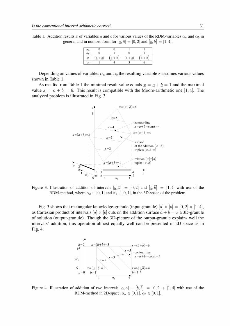
Is the conventional interval arithmetic correct? 31
Table 1. Addition results x of variables a and b for various values of the RDM-variables αa and αb ingeneral and in number-form for [a, a] = [0, 2] and
[b, b
]= [1, 4].
αa 0 0 1 1αb 0 1 0 1
x (a+ b)(a+ b
)(a+ b)
(a+ b
)x 1 4 3 6
Depending on values of variables αa and αb the resulting variable x assumes various valuesshown in Table 1.
As results from Table 1 the minimal result value equals x = a + b = 1 and the maximalvalue x = a + b = 6. This result is compatible with the Moore-arithmetic one [1, 4]. Theanalyzed problem is illustrated in Fig. 3.
Figure 3. Illustration of addition of intervals [a, a] = [0, 2] and[b, b
]= [1, 4] with use of the
RDM-method, where αa ∈ [0, 1] and αb ∈ [0, 1], in the 3D-space of the problem.
Fig. 3 shows that rectangular knowledge-granule (input-granule) [a]× [b] = [0, 2]× [1, 4],as Cartesian product of intervals [a]× [b] cuts on the addition surface a+ b = x a 3D-granuleof solution (output-granule). Though the 3D-picture of the output-granule explains well theintervals’ addition, this operation almost equally well can be presented in 2D-space as inFig. 4.
Figure 4. Illustration of addition of two intervals [a, a] +[b, b
]= [0, 2] + [1, 4] with use of the
RDM-method in 2D-space, αa ∈ [0, 1], αb ∈ [0, 1].

32 Andrzej Piegat, Marek Landowski
The knowledge granule [a]× [b] shown in Fig. 4 is cut by contour lines of constant valuesof sum a + b = x = const, e.g. a + b = 3, a + b = 4, etc. One can easily notice thatthese lines are of different length. The shortest lines are a + b = 1 and a + b = 6 (1-elementsets of solutions). The longest lines are lines corresponding to values x ∈ [3, 4]. Length of acontour line represents measure of a solutions’ set, e.g. length of the line a+ b = 3 representsmeasure of all tuples (a,b) satisfying the condition a + b = 3. The contour-lines’ length canbe interpreted as non-normalized, a priori probability density of the event a+ b = x. Subjectto assumption of the uniform distribution of probability density for variables a and b, on thebasis of Fig. 4 the distribution of a priori probability density for the addition result a+ b = xshown in Fig. 5 can be achieved.
Figure 5. Distribution of a priori probability density (Fig. 5c) of the addition result of two intervalswith use of the RDM-method achieved at assumption of uniform distributions for components a and b
(Fig. 5a and Fig. 5b).
It should be taken into account that the trapezoidal distribution from Fig. 5c was achievedat assumption of uniform distributions for components a and b in situation when experimentaldistributions are not known. Similarly, if for a coin experimental probabilities of head and tailare not known equal a priori probabilities are assumed 0.5 for head and 0.5 for tail. In thecase, when experimental distributions are known then they should be used for determining thedistribution of the sum x = a + b. Let us consider now backward calculations with use ofRDM-variables. As an example of forward calculations the addition problem as below wassolved.
[a, a] +[b, b
]= [0, 2] + [1, 4] = [x, x] = [1, 6]
In frame of backward calculations problem (10) will be considered.
[a, a] + [x, x] = [c, c][0, 2] + [x, x] = [1, 6]
(10)
This problem is illustrated by Fig. 6.As was earlier shown, application of Moore-arithmetic gives the incorrect solution [x, x] =
[1, 4]. Let us now solve this problem with use of the RDM-arithmetic. To this aim RDM-variablesare introduced αa ∈ [0, 1] and αc ∈ [0, 1] and equation (10) is appropriately transformedin (11).
a+ αa (a− a) + x = c+ αc (c− c)0 + 2αa + x = 1 + 5αc
αa ∈ [0, 1], αc ∈ [0, 1](11)

Is the conventional interval arithmetic correct? 33
Figure 6. Illustration of interval backward-calculations where intervals [a, a] and [c, c] are known andinterval [x, x] is not known.
The above equations are usual mathematical equations and can be solved with use ofclassical mathematics. The solution is given by equation (12).
x = c− a+ αc (c− c)− αa (a− a)x = 1 + 5αc − 2αa
αa ∈ [0, 1], αc ∈ [0, 1](12)
Table 2 shows values of the result x for various values of RDM-variables.
Table 2. General and numerical values of the result x of equation [a, a] + [x, x] = [c, c].
αa 0 0 1 1αc 0 1 0 1x (c− a) (c− a) (c− a) (c− a)x 1 6 -1 4
Fig. 7 shows the input granule [a, a]× [c, c] = [0, 2]× [1, 6] in 3D-space A×C, and Fig. 8the output granule in 2D-space: A×X .
Figure 7. Input-(knowledge) granule [a, a]× [c, c] = [0, 2]× [1, 6] in 3D-space A× C.
After projecting the input granule on the functional addition surface a 3D-solution granuleis achieved which is next projected on 2D-surface A×X in Fig. 8.
It should be noticed that after solving equation [0, 2]+[x, x] = [1, 6] with Moore-arithmeticthe 1-dimensional solution ([x, x] = [1, 4]) is obtained. This solution is not complete becauseit does not contain e.g. the test-point TP (0.5, 5) though this point satisfies the consideredequation [0, 2] + [x, x] = [1, 6]. The sum 0.5+ 5.0 = 5.5 is number lying in the interval [1, 6].Instead, solution (12) delivered by the RDM-arithmetic is 2-dimensional because 2 variablesαa and αc occur in it.
x = 1− 2αa + 5αc

34 Andrzej Piegat, Marek Landowski
Figure 8. Solution granule (output granule) of the interval problem [a] + [x] = [c] ([0, 2] + [x, x] =[1, 6]) achieved with use of the interval RDM-arithmetic.
Let us see in Fig. 8 that the solution granule cannot in any way be presented (described) asa 1-dimensional granule [x, x]. Thus, the conventional interval arithmetic is not able to solvebackward-calculations (equation solving). In many cases it delivers false or even paradoxicalsolutions and persons achieving these solutions are not conscious of this fact and use themin real problems. One of false conclusions suggested by Moore-arithmetic is so-called theprinciple of increasing entropy [3].
3. Interval Moore-arithmetic and the principle of increasing entropyLet us once more consider the addition-operation of intervals according to Moore-arithmetic
(13).
[a, a] +[b, b
]=
[a+ b, a+ b
][0, 2] + [1, 4] = [1, 6]
(13)
This operation is illustrated in Fig. 9.
Figure 9. Illustration of the 1-dimensional addition-way of intervals realized by conventionalMoore-arithmetic.
Let us notice that width of the resulting interval [x, x] equal in the considered case to 5 isequal to the sum of widths of the added intervals [a] and [b] i.e. (2+3). The width growingof resulting intervals intuitively is fully understandable and in the subject literature it is calledthe principle of increasing entropy. Further on a quotation from [3] is given.
”. . . the rules of interval mathematics are constructed in such a way that any arithmeticaloperation on intervals results in an interval as well. These rules conform to the well knowncommon view-point that any arithmetical operation with uncertainties should increase thetotal uncertainty (and entropy) of the system”. Now, let us consider the question, whethersuch situation is possible, that after adding two intervals a resulting interval will be achievedwith width that is smaller than widths of two components , i.e. whether a result is possible thatcontradicts the increasing entropy (uncertainty) principle? E.g. is the addition result presentedby (14) possible?
[a] + [x] = [c] = [1, 9] + [x, x] = [11, 12] (14)
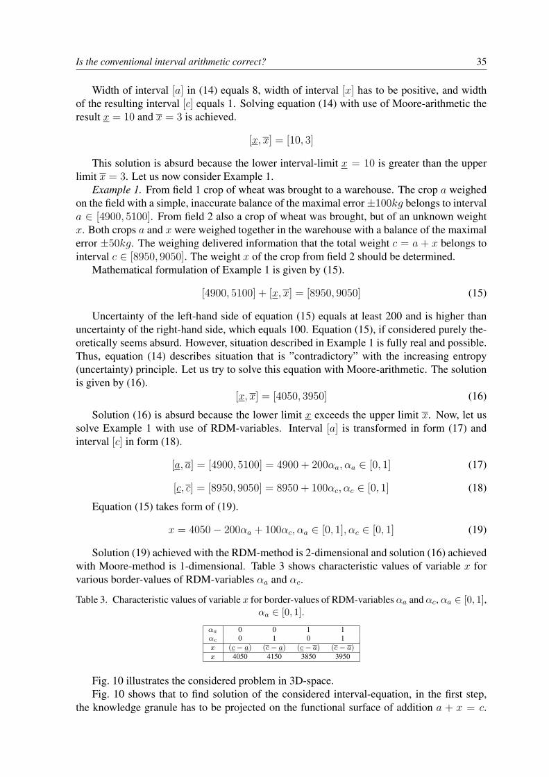
Is the conventional interval arithmetic correct? 35
Width of interval [a] in (14) equals 8, width of interval [x] has to be positive, and widthof the resulting interval [c] equals 1. Solving equation (14) with use of Moore-arithmetic theresult x = 10 and x = 3 is achieved.
[x, x] = [10, 3]
This solution is absurd because the lower interval-limit x = 10 is greater than the upperlimit x = 3. Let us now consider Example 1.
Example 1. From field 1 crop of wheat was brought to a warehouse. The crop a weighedon the field with a simple, inaccurate balance of the maximal error±100kg belongs to intervala ∈ [4900, 5100]. From field 2 also a crop of wheat was brought, but of an unknown weightx. Both crops a and x were weighed together in the warehouse with a balance of the maximalerror ±50kg. The weighing delivered information that the total weight c = a + x belongs tointerval c ∈ [8950, 9050]. The weight x of the crop from field 2 should be determined.
Mathematical formulation of Example 1 is given by (15).
[4900, 5100] + [x, x] = [8950, 9050] (15)
Uncertainty of the left-hand side of equation (15) equals at least 200 and is higher thanuncertainty of the right-hand side, which equals 100. Equation (15), if considered purely the-oretically seems absurd. However, situation described in Example 1 is fully real and possible.Thus, equation (14) describes situation that is ”contradictory” with the increasing entropy(uncertainty) principle. Let us try to solve this equation with Moore-arithmetic. The solutionis given by (16).
[x, x] = [4050, 3950] (16)
Solution (16) is absurd because the lower limit x exceeds the upper limit x. Now, let ussolve Example 1 with use of RDM-variables. Interval [a] is transformed in form (17) andinterval [c] in form (18).
[a, a] = [4900, 5100] = 4900 + 200αa, αa ∈ [0, 1] (17)
[c, c] = [8950, 9050] = 8950 + 100αc, αc ∈ [0, 1] (18)
Equation (15) takes form of (19).
x = 4050− 200αa + 100αc, αa ∈ [0, 1], αc ∈ [0, 1] (19)
Solution (19) achieved with the RDM-method is 2-dimensional and solution (16) achievedwith Moore-method is 1-dimensional. Table 3 shows characteristic values of variable x forvarious border-values of RDM-variables αa and αc.
Table 3. Characteristic values of variable x for border-values of RDM-variables αa and αc, αa ∈ [0, 1],αa ∈ [0, 1].
αa 0 0 1 1αc 0 1 0 1x (c− a) (c− a) (c− a) (c− a)x 4050 4150 3850 3950
Fig. 10 illustrates the considered problem in 3D-space.Fig. 10 shows that to find solution of the considered interval-equation, in the first step,
the knowledge granule has to be projected on the functional surface of addition a + x = c.
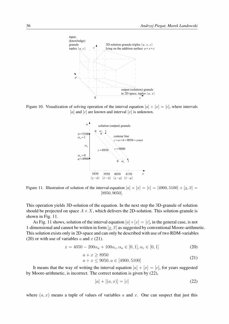
36 Andrzej Piegat, Marek Landowski
Figure 10. Visualization of solving operation of the interval equation [a] + [x] = [c], where intervals[a] and [c] are known and interval [x] is unknown.
Figure 11. Illustration of solution of the interval-equation [a] + [x] = [c] = [4900, 5100] + [x, x] =[8950, 9050].
This operation yields 3D-solution of the equation. In the next step the 3D-granule of solutionshould be projected on space A×X , which delivers the 2D-solution. This solution-granule isshown in Fig. 11.
As Fig. 11 shows, solution of the interval equation [a]+[x] = [c], in the general case, is not1-dimensional and cannot be written in form [x, x] as suggested by conventional Moore-arithmetic.This solution exists only in 2D-space and can only be described with use of two RDM-variables(20) or with use of variables a and x (21).
x = 4050− 200αa + 100αc, αa ∈ [0, 1], αc ∈ [0, 1] (20)
a+ x ≥ 8950a+ x ≤ 9050, a ∈ [4900, 5100]
(21)
It means that the way of writing the interval equation [a] + [x] = [c], for years suggestedby Moore-arithmetic, is incorrect. The correct notation is given by (22),
[a] + [(a, x)] = [c] (22)
where (a, x) means a tuple of values of variables a and x. One can suspect that just this
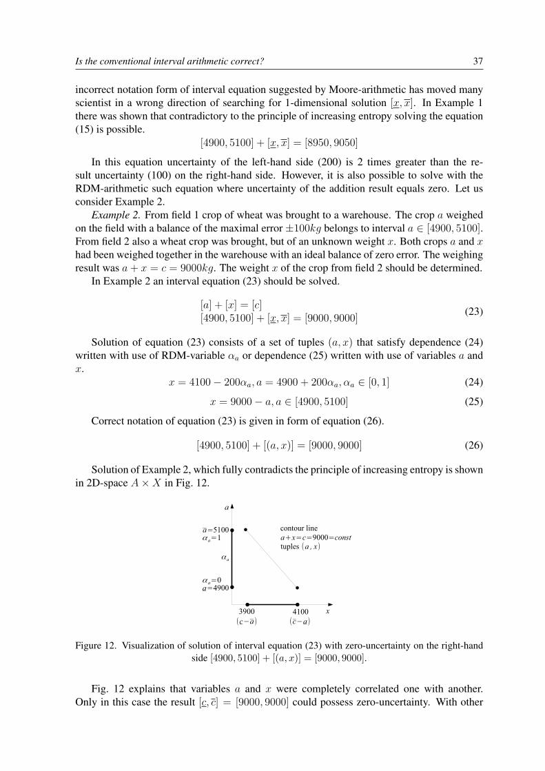
Is the conventional interval arithmetic correct? 37
incorrect notation form of interval equation suggested by Moore-arithmetic has moved manyscientist in a wrong direction of searching for 1-dimensional solution [x, x]. In Example 1there was shown that contradictory to the principle of increasing entropy solving the equation(15) is possible.
[4900, 5100] + [x, x] = [8950, 9050]
In this equation uncertainty of the left-hand side (200) is 2 times greater than the re-sult uncertainty (100) on the right-hand side. However, it is also possible to solve with theRDM-arithmetic such equation where uncertainty of the addition result equals zero. Let usconsider Example 2.
Example 2. From field 1 crop of wheat was brought to a warehouse. The crop a weighedon the field with a balance of the maximal error ±100kg belongs to interval a ∈ [4900, 5100].From field 2 also a wheat crop was brought, but of an unknown weight x. Both crops a and xhad been weighed together in the warehouse with an ideal balance of zero error. The weighingresult was a+ x = c = 9000kg. The weight x of the crop from field 2 should be determined.
In Example 2 an interval equation (23) should be solved.
[a] + [x] = [c][4900, 5100] + [x, x] = [9000, 9000]
(23)
Solution of equation (23) consists of a set of tuples (a, x) that satisfy dependence (24)written with use of RDM-variable αa or dependence (25) written with use of variables a andx.
x = 4100− 200αa, a = 4900 + 200αa, αa ∈ [0, 1] (24)
x = 9000− a, a ∈ [4900, 5100] (25)
Correct notation of equation (23) is given in form of equation (26).
[4900, 5100] + [(a, x)] = [9000, 9000] (26)
Solution of Example 2, which fully contradicts the principle of increasing entropy is shownin 2D-space A×X in Fig. 12.
Figure 12. Visualization of solution of interval equation (23) with zero-uncertainty on the right-handside [4900, 5100] + [(a, x)] = [9000, 9000].
Fig. 12 explains that variables a and x were completely correlated one with another.Only in this case the result [c, c] = [9000, 9000] could possess zero-uncertainty. With other

38 Andrzej Piegat, Marek Landowski
words, variables a and x were ideally fitted one to another. On the other hand, solutionof Example 1 shown in Fig. 11 explains that if uncertainty of the right-hand side of in-terval equation ([4900, 5100] + [(a, x)] = [8950, 9050]) is smaller than uncertainty of theleft-hand side then variables a and x are partly (not fully) correlated (are partly fitted oneto another). Moore-arithmetic is able to correctly solve only such equations [a]+[x]=[c] forwhich 1-dimensional solution [x, x] exists, for case, when both variables a and x are com-pletely not correlated (zero-correlation).
4. Operation of interval subtractionAccording to Moor’s interval arithmetic subtraction of intervals [a] − [b] = [x] should be
realized with use of formula (27).
[a, a]−[b, b
]=
[a− b, a− b
]= [x, x] (27)
Fig. 13 shows a fragment of the subtraction functional-surface a− b = x in 3D-space.
Figure 13. Fragment of the functional subtraction-surface a − b = x with contour-lines of constantdifference values a− b = x = const.
The functional subtraction-surface can be projected from 3D-space into 2D-space (A×B),what is shown in Fig. 14.
Figure 14. Projection of subtraction-surface a−b = x from 3D-space A×B×X (Fig.13) on 2D-spaceA×B.
Let us consider now Example 3 of forward-calculations.
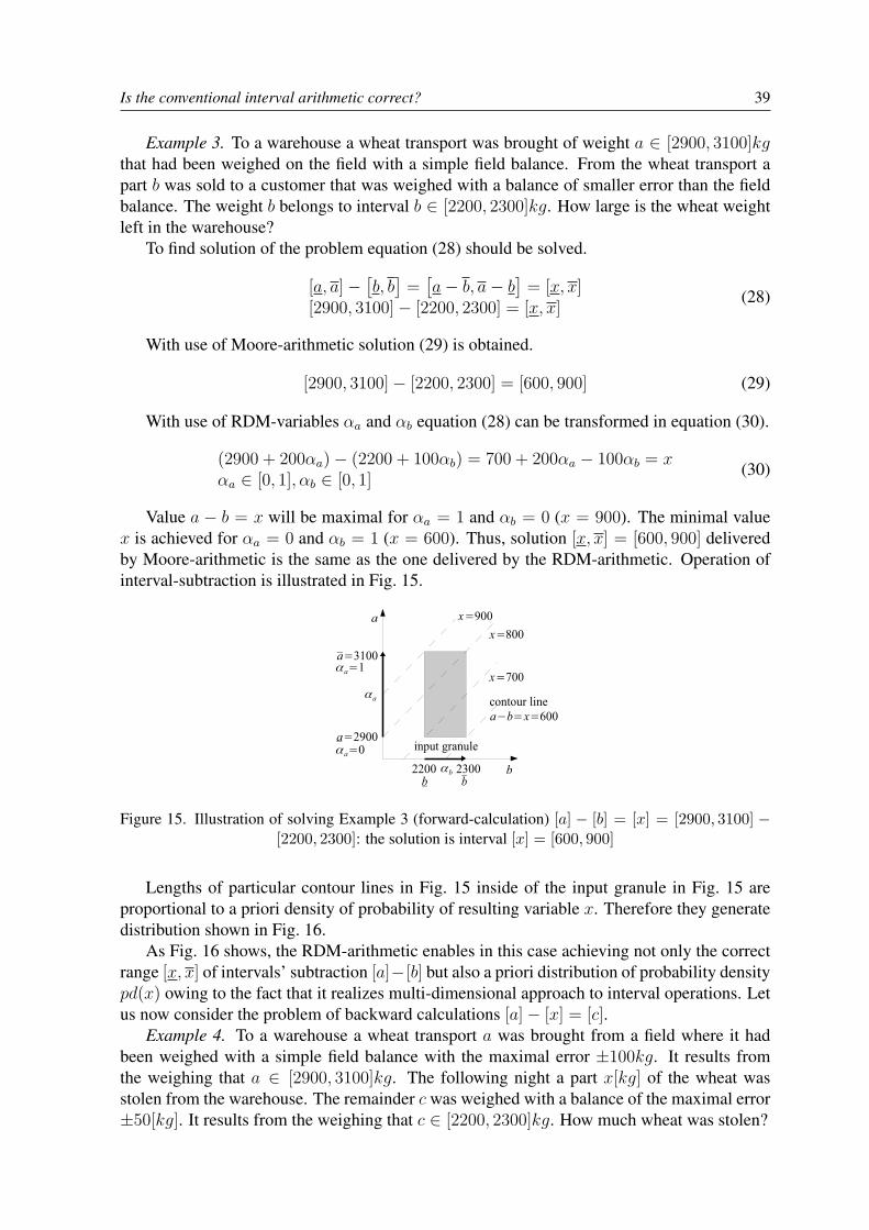
Is the conventional interval arithmetic correct? 39
Example 3. To a warehouse a wheat transport was brought of weight a ∈ [2900, 3100]kgthat had been weighed on the field with a simple field balance. From the wheat transport apart b was sold to a customer that was weighed with a balance of smaller error than the fieldbalance. The weight b belongs to interval b ∈ [2200, 2300]kg. How large is the wheat weightleft in the warehouse?
To find solution of the problem equation (28) should be solved.
[a, a]−[b, b
]=
[a− b, a− b
]= [x, x]
[2900, 3100]− [2200, 2300] = [x, x](28)
With use of Moore-arithmetic solution (29) is obtained.
[2900, 3100]− [2200, 2300] = [600, 900] (29)
With use of RDM-variables αa and αb equation (28) can be transformed in equation (30).
(2900 + 200αa)− (2200 + 100αb) = 700 + 200αa − 100αb = xαa ∈ [0, 1], αb ∈ [0, 1]
(30)
Value a − b = x will be maximal for αa = 1 and αb = 0 (x = 900). The minimal valuex is achieved for αa = 0 and αb = 1 (x = 600). Thus, solution [x, x] = [600, 900] deliveredby Moore-arithmetic is the same as the one delivered by the RDM-arithmetic. Operation ofinterval-subtraction is illustrated in Fig. 15.
Figure 15. Illustration of solving Example 3 (forward-calculation) [a] − [b] = [x] = [2900, 3100] −[2200, 2300]: the solution is interval [x] = [600, 900]
Lengths of particular contour lines in Fig. 15 inside of the input granule in Fig. 15 areproportional to a priori density of probability of resulting variable x. Therefore they generatedistribution shown in Fig. 16.
As Fig. 16 shows, the RDM-arithmetic enables in this case achieving not only the correctrange [x, x] of intervals’ subtraction [a]−[b] but also a priori distribution of probability densitypd(x) owing to the fact that it realizes multi-dimensional approach to interval operations. Letus now consider the problem of backward calculations [a]− [x] = [c].
Example 4. To a warehouse a wheat transport a was brought from a field where it hadbeen weighed with a simple field balance with the maximal error ±100kg. It results fromthe weighing that a ∈ [2900, 3100]kg. The following night a part x[kg] of the wheat wasstolen from the warehouse. The remainder c was weighed with a balance of the maximal error±50[kg]. It results from the weighing that c ∈ [2200, 2300]kg. How much wheat was stolen?

40 Andrzej Piegat, Marek Landowski
Figure 16. Distribution of a priori density of probability (pd) of subtraction result of two intervals withthe RDM-arithmetic subject to uniform distributions pd(a) and pd(b).
To answer the question with use of Moore-arithmetic equation (31) is to be solved.
[2900, 3100]− [x, x] = [2200, 2300] (31)
Solution of equation (31) is given by (32).
2900− x = 2200, x = 7003100− x = 2300, x = 800[x, x] = [800, 700]
(32)
Solution (32) is absurd because x > x that can be interpreted as negative width (x− x =700− 800 = −100) of the interval or negative entropy [3]. Now, let us solve Example 4 withuse of the RDM-arithmetic. Interval [a] can be written as
a = 2900 + 200αa, αa ∈ [0, 1].
Interval [c] can be written as
c = 2200 + 100αc, αc ∈ [0, 1].
And equation (31) can be written in form of (33)
(2900 + 200αa)− x = 2200 + 100αc
x = 700 + 200αa − 100αc, αa ∈ [0, 1], αc ∈ [0, 1](33)
Equation (33) is the mathematical solution of the problem. Table 4 shows values of vari-able x for various border values of αa and αc.
Table 4. Values of variable x for various border-values of RDM-variables αa and αc and correspondingvalues of variables a and c.αa 0 0 1 1αc 1 0 1 0x 600 700 800 900a 2900 2900 3100 3100c 2300 2200 2300 2200x 600 700 800 900
Fig. 17 presents solution granule of equation [2900, 3100] − [(a, x)] = [2200, 2300] fromExample 4.
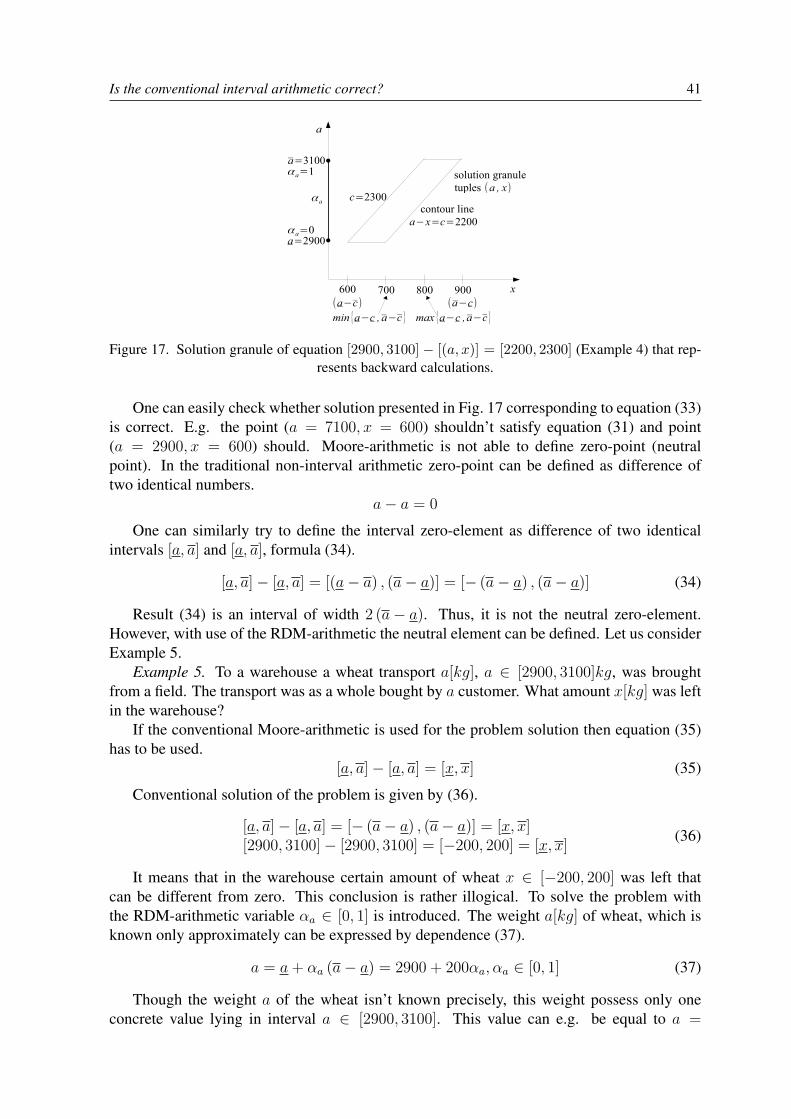
Is the conventional interval arithmetic correct? 41
Figure 17. Solution granule of equation [2900, 3100] − [(a, x)] = [2200, 2300] (Example 4) that rep-resents backward calculations.
One can easily check whether solution presented in Fig. 17 corresponding to equation (33)is correct. E.g. the point (a = 7100, x = 600) shouldn’t satisfy equation (31) and point(a = 2900, x = 600) should. Moore-arithmetic is not able to define zero-point (neutralpoint). In the traditional non-interval arithmetic zero-point can be defined as difference oftwo identical numbers.
a− a = 0
One can similarly try to define the interval zero-element as difference of two identicalintervals [a, a] and [a, a], formula (34).
[a, a]− [a, a] = [(a− a) , (a− a)] = [− (a− a) , (a− a)] (34)
Result (34) is an interval of width 2 (a− a). Thus, it is not the neutral zero-element.However, with use of the RDM-arithmetic the neutral element can be defined. Let us considerExample 5.
Example 5. To a warehouse a wheat transport a[kg], a ∈ [2900, 3100]kg, was broughtfrom a field. The transport was as a whole bought by a customer. What amount x[kg] was leftin the warehouse?
If the conventional Moore-arithmetic is used for the problem solution then equation (35)has to be used.
[a, a]− [a, a] = [x, x] (35)
Conventional solution of the problem is given by (36).
[a, a]− [a, a] = [− (a− a) , (a− a)] = [x, x][2900, 3100]− [2900, 3100] = [−200, 200] = [x, x]
(36)
It means that in the warehouse certain amount of wheat x ∈ [−200, 200] was left thatcan be different from zero. This conclusion is rather illogical. To solve the problem withthe RDM-arithmetic variable αa ∈ [0, 1] is introduced. The weight a[kg] of wheat, which isknown only approximately can be expressed by dependence (37).
a = a+ αa (a− a) = 2900 + 200αa, αa ∈ [0, 1] (37)
Though the weight a of the wheat isn’t known precisely, this weight possess only oneconcrete value lying in interval a ∈ [2900, 3100]. This value can e.g. be equal to a =
42 Andrzej Piegat, Marek Landowski
2951.67132 . . . kg. Independently of what amount a[kg] had been brought to the warehousefrom the field, the same amount a[kg] was taken by the customer. Thus, zero kg of wheat wasleft in the warehouse and, correctly, the problem should be expressed by dependence (38).
[a]− [a] = [a+ αa (a− a)]− [a+ αa (a− a)] = 0, αa ∈ [0, 1] (38)
Summarizing: there are problems in which difference of two identical intervals is preciselyequal to zero and there are problems in which difference of two identical intervals is not equalto zero and is represented by an interval [x, x]. This fact means a great difference betweenthe classical singleton-mathematics and the interval mathematics. Calculation results of thesingleton-mathematics are general and problem-independent. However, in case of intervalmathematics calculation results are problem-dependent. Thus, interval mathematics is muchmore difficult and complicated than singleton-mathematics. In Example 6 a problem will beshown, where difference of two identical intervals is not equal to zero.
Example 6. Boxer A and boxer B before fight were weighed with a balance of maximalerror±0.5kg. In case of both boxers the balance shown the same value of 85kg. It means thatthe real weight a of boxer A lies in interval a ∈ [84.5, 85.5] and the real weight b of boxerB also lies in the same interval b ∈ [84.5, 85.5]. How large is the weight difference betweenboxer A and B?
To determine this difference the difference of two intervals should be found as below.
[a, a]−[b, b
]= [84.5, 85.5]− [84.5, 85.5]
Weight of each boxer has a concrete value. Weight of boxer A can be e.g. a = 84.791 . . . kgand of boxer B can be e.g. b = 85.123 . . . kg. Probability that both weights are ideally equalis infinitely small. Weight of boxer A can be written as below.
a = a+ αa (a− a) = 84.5 + αa, αa ∈ [0, 1]
Weight of boxer B can be written as
b = b+ αb
(b− b
)= 84.5 + αb, αb ∈ [0, 1]
Thus, the weight difference is determined by formula (39).
[a]− [b] = 84.5 + αa − 84.5− αb, αa ∈ [0, 1], αb ∈ [0, 1][a]− [b] = αa − αb
[a]− [b] = [−1, 1](39)
It means that the maximal weight-difference of the boxers can reach even 1kg, in spiteof the fact that the balance shown the same weight of 85kg for both boxers. SummarizingExample 5 and Example 6 one can say that in case of interval arithmetic it is not possible togive one general formula as in the traditional singleton-arithmetic (e.g. a− a = 0, 5− 5 = 0)for subtraction of two identical intervals (e.g. [a]− [a] = [2, 3]− [2, 3]) that would be correctin all cases. In each real problem one should consider whether the real (not precisely but onlyapproximately known) subtracted values a − b, represented by intervals [a, a] and
[b, b
]are
identical or different. Thus, interval arithmetic is much more complicated than the arithmeticof precise, non-interval numbers.
Is the conventional interval arithmetic correct? 43
5. ConclusionsThe paper presented a new (according to authors’ knowledge) multi-dimensional inter-
val arithmetic based on RDM-variables for case of addition and subtraction (because of thepaper-volume limitation). Operations of multiplication and division will be described innext paper of authors. There was shown, that uncertain, approximate parameters of a sys-tem model increase its dimensionality what next increases calculation difficulties. However,the RDM-arithmetic allows for correct solutions of such problems, which can not be solvedby Moore’s interval arithmetic. It was shown in the paper that the principle of increasingentropy (uncertainty) of interval calculations is generally not true. It also was shown thatinterval arithmetic mainly realizes the task of function-extrema determining in a constrainedgranule-space. The RDM-arithmetic operations presented in the paper are only beginningof large investigations that will lead to a new multidimensional interval-mathematics whichenables solving many complicated problems containing uncertainty and approximate data,especially problems of artificial intelligence, fuzzy mathematics, probabilistic mathematics,Computing with Words etc. Especially the α-cut method used in fuzzy arithmetic will requirea revision to correctly solve equations.
References[1] Aliev, R., Pedrycz, W., Fazlollahi, B., Huseynov, O., Alizadeh, A., Guirimov, B. (2012). Fuzzy
logic-based generalized decision theory with imperfect information, Information Sciences 189,18–42.
[2] Bronstein, I.N., et al. (2004). Modern compendium of mathematics, (in Polish), WydawnictwoNaukowe PWN, Warszawa, Poland.
[3] Dymova, L. (2011). Soft computing in economics and finance, Springer–Verlag, Berlin, Heidel-berg.
[4] Hanss, M. (2005). Applied fuzzy arithmetic, Springer–Verlag, Berlin, Heidelberg.[5] Jaroszewicz, S., Korzen, M. (2012a). Arithmetic operations on independent random variables: a
numerical approach, SIAM Journal of Scientific Computing, vol. 34, No. 4, pp A1241-A1265.[6] Jaroszewicz, S., Korzen, M. (2012b). Pacal: A python package for arithmetic computations with
random variables, http://pacal.sourceforge.net/, on line: September 2012.[7] Kaufmann, A., Gupta, M.M. (1991). Introduction to fuzzy arithmetic, Van Nostrand Reinhold,
New York.[8] Liu, S., Lin Forrest, J.Y. (2010). Grey systems, theory and applications. Springer, Berlin, Heidel-
berg.[9] Moore, R.E. (1966). Interval analysis, Prentice Hall, Englewood Cliffs N.J.
[10] Moore, R.E., Kearfott, R.B., Cloud. M.J. (2009). Introduction to interval analysis. SIAM,Philadelphia.
[11] Pedrycz, W., Skowron A., Kreinovicz, V. (eds) (2008). Handbook of granular computing. Wiley,Chichester, England.
[12] Piegat, A. (2001). Fuzzy control and modeling, Springer–Verlag, Heidelberg, New York.[13] Sengupta, A., Pal, T.K. (2009). Fuzzy preference ordering of interval numbers in decision prob-
lems. Springer, Berlin, Heidelberg.[14] Sevastjanov, P., Dymova, L. (2009). A new method for solving interval and fuzzy equations:
linear case, Information Sciences 17, 925–937.[15] Sevastjanov, P., Dymova, L., Bartosiewicz, P. (2012). A framework for rule-base evidential rea-
soning in the interval settings applied to diagnosing type 2 diabets, Expert Systems with Appli-cations 39, 4190–4200.

44 Andrzej Piegat, Marek Landowski
[16] Williamson, R. (1989). Probabilistic arithmetic, Ph.D. thesis, Department of Electrical Engineer-ing, University of Queensland.
[17] Zadeh, L.A. (2002). From computing with numbers to computing with words – from manipula-tion of measurements to manipulation of perceptions. International Journal of Applied Mathe-matics and Computer Science, Vol.12, No.3, 307–324.

Journal of Theoretical and Applied Computer Science Vol. 6, No. 2, 2012, pp. 45–59ISSN 2299-2634 http://www.jtacs.org
Classification based 3-D surface analysis: predictingspringback in sheet metal forming
M. Sulaiman Khan, Frans Coenen, Clare Dixon, Subhieh El-SalhiDepartment of Computer Science, University of Liverpool, United Kingdom{mskhan,coenen,cldixon,salhi}@liverpool.ac.uk
Abstract: This paper describes an application of data mining, namely classification, with respect to 3-Dsurface analysis. More specifically in the context of sheet metal forming, especially AsymmetricIncremental Sheet Forming (AISF). The issue with sheet metal forming processes is that their ap-plication results in springback, which means that the resulting shape is not necessarily the desiredshape. Errors are introduced in a non-linear manner for a variety of reasons, but the main con-tributor is the geometry of the desired shape. A Local Geometry Matrix (LGM) representation isthus proposed that allows the capture of local 3-D surface geometries in such a way that classifiergenerators can be effectively applied. The resulting classifier can then be used to predict errorswith respect to new surfaces to be manufactured so that some correcting strategy can be applied.The reported evaluation of the proposed technique indicates that excellent results can be produced.
Keywords: classification, prediction, 3-D surface modelling
1. IntroductionData Mining classification techniques have been applied in many domains using a variety
of classifier generators. Much of the original work was directed at the classification of tabulardata. Subsequent work focused on more ambitious forms of data such a text, graph and imageclassification. The current focus is on even more challenging forms of data such as video and3-D volumes. The work described in this paper is concerned with 3-D surface classification.The challenge with these different forms of classification is not the classification techniquesthat are used, these tend to be well established, but on the nature of the data preprocessingrequired to convert the data into a form suited to the application of classifier generators. Thedata needs to be translated into a format that captures the salient features of the data but at thesame time support efficient processing.
In this paper we propose a method for capturing the nature (geometry) of 3-D surfacesin such a way that classification can be applied. More specifically we are interested in datamining techniques for identifying correlations between 3-D surfaces, and then to predict likelycorrelations with respect to “new” 3-D surfaces. To act as a focus for the work the investi-gation is directed at predicting the springback that occurs during Asymmetric IncrementalSheet Forming (AISF); a manufacturing process used to shape sheet metal. The advantagesof AISF are that it is comparatively inexpensive and does not require heating of the metal(heating introduces potential fracture points and adds an additional financial overhead). Thedisadvantage of AISF metal forming is that springback is introduced into the shape. TheAISF process commences with a desired input shape, defined in terms of a set of 3-D coor-dinates, and produces an output shape which, as a result of the process, is a “variation” of
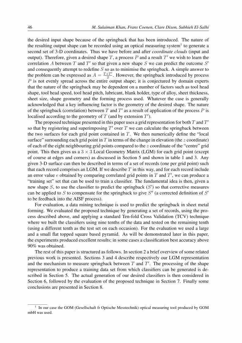
46 M. Sulaiman Khan, Frans Coenen, Clare Dixon, Subhieh El-Salhi
the desired input shape because of the springback that has been introduced. The nature ofthe resulting output shape can be recorded using an optical measuring system1 to generate asecond set of 3-D coordinates. Thus we have before and after coordinate clouds (input andoutput). Therefore, given a desired shape T , a process P and a result T ′ we wish to learn thecorrelation A between T and T ′ so that given a new shape S we can predict the outcome S ′
and consequently attempt to redefine S so as to minimise the springback. A simple answer tothe problem can be expressed as A = T+T ′
2. However, the springback introduced by process
P is not evenly spread across the entire output shape; it is conjectured by domain expertsthat the nature of the springback may be dependent on a number of factors such as tool headshape, tool head speed, tool head pitch, lubricant, blank holder, type of alloy, sheet thickness,sheet size, shape geometry and the forming process used. Whatever the case is generallyacknowledged that a key influencing factor is the geometry of the desired shape. The natureof the springback (correlation) between T and T ′ as a result of application of the process P islocalised according to the geometry of T (and by extension T ′).
The proposed technique presented in this paper uses a grid representation for both T and T ′
so that by registering and superimposing T ′ over T we can calculate the springback betweenthe two surfaces for each grid point contained in T . We then numerically define the “localsurface” surrounding each grid point in T in terms of the change in elevation (the z coordinate)of each of the eight neighbouring grid points compared to the z coordinate of the “centre” gridpoint. This then gives us a 3 × 3 Local Geometry Matrix (LGM) for each grid point (exceptof course at edges and corners) as discussed in Section 5 and shown in table 1 and 3. Anygiven 3-D surface can then be described in terms of a set of records (one per grid point) suchthat each record comprises an LGM. If we describe T in this way, and for each record includean error value e obtained by comparing correlated grid points in T and T ′, we can produce a“training set” set that can be used to train a classifier. The fundamental idea is then, given anew shape S, to use the classifier to predict the springback (S ′) so that corrective measurescan be applied to S to compensate for the springback to give S ′′ (a corrected definition of S ′
to be feedback into the AISF process).For evaluation, a data mining technique is used to predict the springback in sheet metal
forming. We evaluated the proposed technique by generating a set of records, using the pro-cess described above, and applying a standard Ten-fold Cross Validation (TCV) techniquewhere we built the classifiers using nine tenths of the data and tested on the remaining tenth(using a different tenth as the test set on each occasion). For the evaluation we used a largeand a small flat topped square based pyramid. As will be demonstrated later in this paper,the experiments produced excellent results; in some cases a classification best accuracy above90% was obtained.
The rest of this paper is structured as follows. In section 2 a brief overview of some relatedprevious work is presented. Sections 3 and 4 describe respectively our LGM representationand the mechanism to measure springback between T and T ′. The processing of the shaperepresentation to produce a training data set from which classifiers can be generated is de-scribed in Section 5. The actual generation of our desired classifiers is then considered inSection 6, followed by the evaluation of the proposed technique in Section 7. Finally someconclusions are presented in Section 8.
1 In our case the GOM (Gesellschaft fr Optische Messtechnik) optical measuring tool produced by GOMmbH was used.
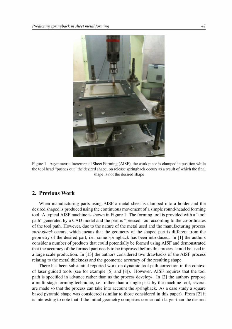
Predicting springback in sheet metal forming 47
Figure 1. Asymmetric Incremental Sheet Forming (AISF), the work piece is clamped in position whilethe tool head “pushes out” the desired shape, on release springback occurs as a result of which the final
shape is not the desired shape
2. Previous Work
When manufacturing parts using AISF a metal sheet is clamped into a holder and thedesired shaped is produced using the continuous movement of a simple round-headed formingtool. A typical AISF machine is shown in Figure 1. The forming tool is provided with a “toolpath” generated by a CAD model and the part is “pressed” out according to the co-ordinatesof the tool path. However, due to the nature of the metal used and the manufacturing processspringback occurs, which means that the geometry of the shaped part is different from thegeometry of the desired part, i.e. some springback has been introduced. In [1] the authorsconsider a number of products that could potentially be formed using AISF and demonstratedthat the accuracy of the formed part needs to be improved before this process could be used ina large scale production. In [13] the authors considered two drawbacks of the AISF processrelating to the metal thickness and the geometric accuracy of the resulting shape.
There has been substantial reported work on dynamic tool path correction in the contextof laser guided tools (see for example [5] and [8]). However, AISF requires that the toolpath is specified in advance rather than as the process develops. In [2] the authors proposea multi-stage forming technique, i.e. rather than a single pass by the machine tool, severalare made so that the process can take into account the springback. As a case study a squarebased pyramid shape was considered (similar to those considered in this paper). From [2] itis interesting to note that if the initial geometry comprises corner radii larger than the desired
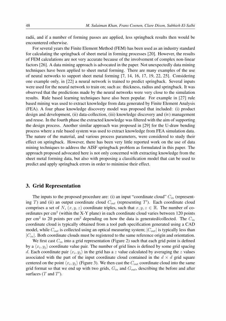
48 M. Sulaiman Khan, Frans Coenen, Clare Dixon, Subhieh El-Salhi
radii, and if a number of forming passes are applied, less springback results then would beencountered otherwise.
For several years the Finite Element Method (FEM) has been used as an industry standardfor calculating the springback of sheet metal in forming processes [20]. However, the resultsof FEM calculations are not very accurate because of the involvement of complex non-linearfactors [26]. A data mining approach is advocated in the paper. Not unexpectedly data miningtechniques have been applied to sheet metal forming. There are many examples of the useof neural networks to support sheet metal forming [7, 14, 16, 17, 19, 22, 25]. Consideringone example only, in [22] a neural network is trained to predict springback. Several inputswere used for the neural network to train on; such as: thickness, radius and springback. It wasobserved that the predictions made by the neural networks were very close to the simulationresults. Rule based learning techniques have also been popular. For example in [27] rulebased mining was used to extract knowledge from data generated by Finite Element Analysis(FEA). A four phase knowledge discovery model was proposed that included: (i) productdesign and development, (ii) data-collection, (iii) knowledge discovery and (iv) managementand reuse. In the fourth phase the extracted knowledge was filtered with the aim of supportingthe design process. Another similar approach was proposed in [29] for the U-draw bendingprocess where a rule based system was used to extract knowledge from FEA simulation data.The nature of the material, and various process parameters, were considered to study theireffect on springback. However, there has been very little reported work on the use of datamining techniques to address the AISF springback problem as formulated in this paper. Theapproach proposed advocated here is not only concerned with extracting knowledge from thesheet metal forming data, but also with proposing a classification model that can be used topredict and apply springback errors in order to minimise their effect.
3. Grid Representation
The inputs to the proposed procedure are: (i) an input “coordinate cloud” Cin (represent-ing T ) and (ii) an output coordinate cloud Cout (representing T ′). Each coordinate cloudcomprises a set of N , (x, y, z) coordinate triples, such that x, y, z ∈ R. The number of co-ordinates per cm2 (within the X-Y plane) in each coordinate cloud varies between 120 pointsper cm2 to 20 points per cm2 depending on how the data is generated/collected. The Cin
coordinate cloud is typically obtained from a tool path specification generated using a CADmodel, while Cout is collected using an optical measuring system; |Cout| is typically less than|Cin|. Both coordinate clouds must be registered to the same reference origin and orientation.
We first cast Cin into a grid representation (Figure 2) such that each grid point is definedby a 〈xi, yj〉 coordinate value pair. The number of grid lines is defined by some grid spacingd. Each coordinate pair 〈xi, yj〉 in the grid has a z value calculated by averaging the z valuesassociated with the part of the input coordinate cloud contained in the d × d grid squarecentered on the point 〈xi, yj〉 (Figure 3). We then cast the Cout coordinate cloud into the samegrid format so that we end up with two grids, Gin and Gout, describing the before and aftersurfaces (T and T ′).

Predicting springback in sheet metal forming 49
Figure 2. Example grid referenced to a centralorigin (grid spacing = d)
Figure 3. Coordinate cloud points associatedwith a grid point 〈xi, yj〉
4. Springback MeasurementA simple mechanism for establishing the degree of springback (e) at a particular grid point
is simply to measure difference between the z values in Gin and Gout (Figure 4). However, amore accurate measure is to determine the length of the surface normal from each grid pointin Gin to the point where it intersects Gout. The distance between any two three dimensionalpoints can be calculated using the point to point Euclidean distance formula:
d =√
(x2 − x1)2 + (y2 − y1)2 + (z2 − z1)2 (1)
Figure 4. Cross section at a grid line showing simple vertical springback error calculation between abefore and after shape
However, the application of equation (1) first requires knowledge of the x, y, z coordinates ofthe point where the normal intersects Gout. With respect to the work described in this paperwe have used the line plane intersection method [9] to determine the length of the normalbetween two surfaces. Using this approach we find the normal to a plane by calculating thecross product of two orthogonal vectors contained within the plane. Once we have the normalwe can calculate the equation for the line that includes the start and end points of the normaland then determine the point at which this line cuts Gout. We can then calculate the length ofthe normal separating the two planes. The process is as follows (with reference to Figure 5):
1. For each grid point in Gin first identify the four neighbouring grid points in the X and Yplanes as shown in Figure 5 (except at edges and corners where three and two neigbouringgrid points will be identified respectively).
2. Define a set of four vectors V = {v1, . . . , v4} = {〈p∅, p1〉, 〈p∅, p2〉, 〈p∅, p3〉, 〈p∅, p4〉},each described in terms of its x−y−z distance from p∅ (the origin for the vector system).

50 M. Sulaiman Khan, Frans Coenen, Clare Dixon, Subhieh El-Salhi
Figure 5. Error calculation using the line plane intersection method
3. Using the four vectors in V , four surface normals are calculated, N = {n1 . . . n4}, bydetermine the cross product between each pair of vectors: v1×v2, v2×v3, v3×v4, v4×v1.(Note that to validate a surface normal ni, the dot product of one of its associated vectorsvj and ni must be equal to zero, ni · vj = 0.)
4. For each normal n1 . . . n4 calculate the local plane equation in Gin that includes P∅ (thususing, in turn, points {p1, p∅, p2}, {p2, p∅, p3}, {p3, p∅, p4} and {p4, p∅, p1}). The planeequation is given by Equation 2.
ax+ by + cz + d = 0 (2)
5. For each plane equation identified in (4) determine the parametric equations (a set ofequations/functions which describe the x, y and z coordinates of the graph of some linein a plane) [9] of the surface normal as a straight line according to the identities given inequation 3.
x = a+ i(t), y = b+ j(t), z = c+ k(t) (3)
where t is a constant; a, b and c are the x-y-z coordinates for the point p∅; and i, j andk are the normal components. The constant t is calculated by substituting the parametricequations in plane equation 2 for x, y and z.
6. Once the parametric equations for each surface normal are found, they are then used tocompute the points of intersection of each normal with Gout.
7. We then use the coordinates for each of the four points of intersection and p∅ to calculatethe Euclidean distance (the error) between p∅ and each intersection point to give four errorvalues E = {e1 . . . e4}
8. We then assign each error a direction (-ve or +ve) based on the direction of the springback.If springback is “downwards”, a -ve direction is assigned to the error. Similarly if thespringback is “upwards” a +ve direction is assigned to the error. Note that for each pointthe direction for each of the four errors is same.
9. We now have four error values for each grid point (except at the corners and edges wherewe will have two or three respectively), we then find the “overall” error e simply by se-lecting the minimum error that is nearest to zero. The reason for selecting the minimalerror is that it gives us the nearest point to the before surface.
On completion of the process our input grid, Gin, will comprise a set of (x, y, z) coordinatesdescribing the N grid points, each with an associated springback (error) value e.

Predicting springback in sheet metal forming 51
5. Surface Representation (The Local Geometry Matrix)In this section we describe how local geometries can be represented using the concept of
a Local Geometry Matrix (LGM). From the foregoing it has already been noted that the valueof e is particularly influenced by the nature of the geometry of the desired surface (shape).We can model this according to the change in the δz value of the eight grid points surround-ing each grid point. (Of course along the edges and at the corners of the grid we will havefewer neighbouring grid points). Thus we generate n records (where n is the number of gridpoints) each typically comprising nine values, eight δz values and an associate e value. We,then coarsen the δz values by describing them using qualitative labels taken from a set L todescribe the nature of the “slope” in each of the eight neighbouring directions. Therefore wecan describe |L|8 different “local geometries” if we take orientation into consideration. Thusif we have a label set {negative, level, positive} we can describe 38 = 6561 different localgeometries.
Example 1. Considering the flattened square based pyramid shape in Figure 6 and a sectionof the surface, measuring 3× 3 grid points, covering an edge as shown, then the z coordinatematrix associated with the grid point might be as shown in Table 1. The δz values are thencalculated by subtracting the centre z value from each of the surrounding z values in turn.With respect to the example the δz matrix result would be as shown in Table 2 (the centre gridreference point always has a value of 0). We refer to this matrix as a Local Geometry Matrix(LGM). Assuming L = {negative, level, positive}, and ordering the matrix elements (gridpoints) in a clockwise direction from the top left, would give us a record of the following formwhere e is the error value associated with the grid point that the record describes:
(positive, positive, positive, level, negative, negative, negative, level, e)
where e is the error value.
Figure 6. Square Based Pyramid With Side Sec-tion (Example 1)
Figure 7. Square Based Pyramid With CornerSection (Example 2)
20 20 2010 10 100 0 0
Table 1. Z matrix for Example 1
10 10 100 0 0
-10 -10 -10
Table 2. LGM for Example 1

52 M. Sulaiman Khan, Frans Coenen, Clare Dixon, Subhieh El-Salhi
Example 2. Again considering a flattened square based pyramid shape but now looking at asection of the surface, measuring 3×3 grid points, located at the corner of the shape as shownin Figure 7, the z coordinates associated with the grid point might be as shown in Table 3. TheLGM would then be as shown in Table 4. Again assuming L = {negative, level, positive}the resulting record would be:
(positive, level, negative, negative, negative, negative, negative, level, e)
20 10 010 10 00 0 0
Table 3. Z matrix for Example 2
10 0 -100 0 -10
-10 -10 -10
Table 4. LGM for Example 2
The proposed representation can be used to capture all local geometries. Given a suitabletest shapes (in this paper we have used two flattened square based pyramid shapes, one sub-stantially larger than the other) we can associate an error value with every possible geometry.It should be noted that, at least conceptually, the use of LGMs is akin to the use of LocalBinary Patterns (LBPs) as applied in the context of image texture analysis [12, 21].
The set of error values was also discretised using a number of qualitative labels eachdescribing a particular sub-range of error values. The sub-ranges used were of equal sizeand designed to encompass the full range of error values from the recorded minimum to therecorded maximum.
6. Classifier GenerationThere are a number of classification mechanisms that can be applied to data pre-processed
in the manner described above, so as to generate a classifier that can be applied to unseen data.In the work described here we favour a classifier that generates rules. Rule base representa-tions offer two principal advantages:
1. Rule representations are intuitive; they are simple to interpret and understand.2. Because of (1), the validity of rules can be easily verified by domain experts.
It is possible to generate rules using many of the available classifier generation techniques,although some are more suited to rule generation than others. Classification Association Rule(CAR) generators directly generate rule sets. There are a number of well established CARMining (CARM) algorithms that can be adopted: examples include CPAR [28], CMAR [18]and TFPC [3, 4]. Although the principle is the same each of these operates in slightly differentmanner. It is also fairly straightforward to generate rule sets using decision tree classifiers suchas the ID3 Algorithm [24], C4.5 [23] or the MARS Algorithm [11]. Generating rules fromNeural Network based classification techniques or Support Vector Machines is less straightforward but can be done [10, 6]. Regardless of the classification algorithm adopted it wasassumed that the required input would be in the form of a set of binary valued attributes. Thusfor our representation (as describbed above) we will use |L| × 8 attributes plus a number oferror attributes. Thus if |L| = 5 the input training data will comprise 45 columns, 5 × 8attributes plus the class (error) attributes.
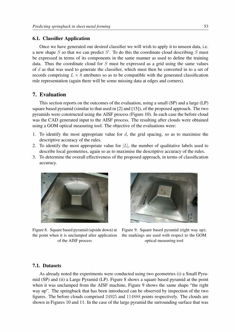
Predicting springback in sheet metal forming 53
6.1. Classifier ApplicationOnce we have generated our desired classifier we will wish to apply it to unseen data, i.e.
a new shape S so that we can predict S ′. To do this the coordinate cloud describing S mustbe expressed in terms of its components in the same manner as used to define the trainingdata. Thus the coordinate cloud for S must be expressed as a grid using the same valuesof d as that was used to generate the classifier, which must then be converted in to a set ofrecords comprising L × 8 attributes so as to be compatible with the generated classificationrule representation (again there will be some missing data at edges and corners).
7. EvaluationThis section reports on the outcomes of the evaluation, using a small (SP) and a large (LP)
square based pyramid (similar to that used in [2] and [15]), of the proposed approach. The twopyramids were constructed using the AISF process (Figure 10). In each case the before cloudwas the CAD generated input to the AISF process. The resulting after clouds were obtainedusing a GOM optical measuring tool. The objective of the evaluations were:
1. To identify the most appropriate value for d, the grid spacing, so as to maximise thedescriptive accuracy of the rules.
2. To identify the most appropriate value for |L|, the number of qualitative labels used todescribe local geometries, again so as to maximise the descriptive accuracy of the rules.
3. To determine the overall effectiveness of the proposed approach, in terms of classificationaccuracy.
Figure 8. Square based pyramid (upside down) atthe point when it is unclamped after application
of the AISF process
Figure 9. Square based pyramid (right way up);the markings are used with respect to the GOM
optical measuring tool
7.1. DatasetsAs already noted the experiments were conducted using two geometries (i) a Small Pyra-
mid (SP) and (ii) a Large Pyramid (LP). Figure 8 shows a square based pyramid at the pointwhen it was unclamped from the AISF machine, Figure 9 shows the same shape “the rightway up”. The springback that has been introduced can be observed by inspection of the twofigures. The before clouds comprised 24925 and 114888 points respectively. The clouds areshown in Figures 10 and 11. In the case of the large pyramid the surrounding surface that was
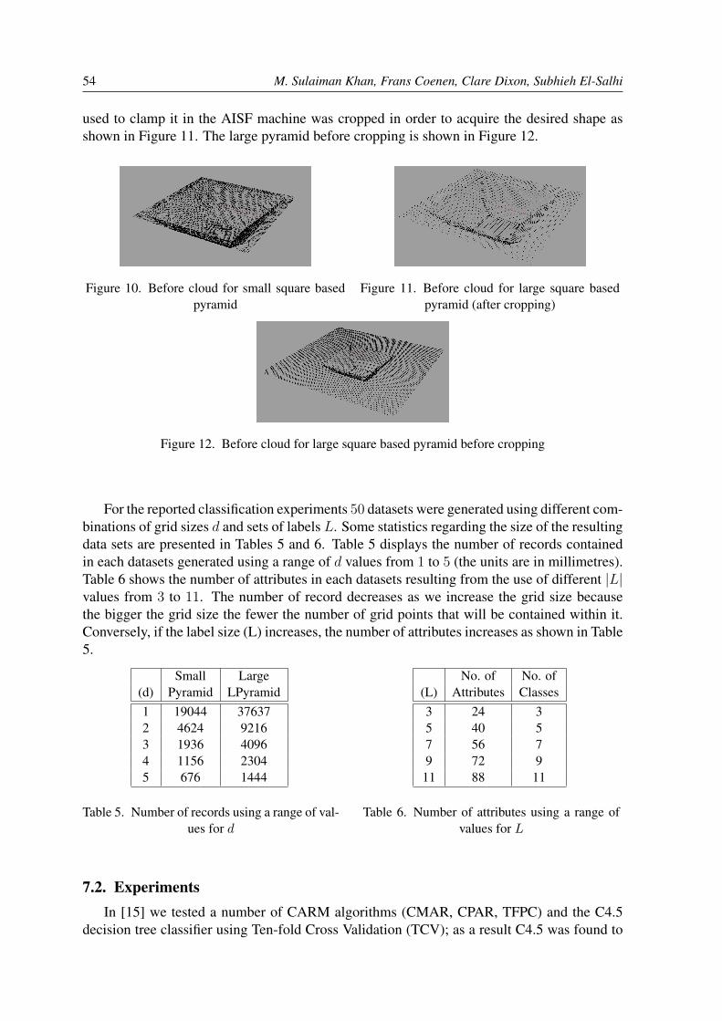
54 M. Sulaiman Khan, Frans Coenen, Clare Dixon, Subhieh El-Salhi
used to clamp it in the AISF machine was cropped in order to acquire the desired shape asshown in Figure 11. The large pyramid before cropping is shown in Figure 12.
Figure 10. Before cloud for small square basedpyramid
Figure 11. Before cloud for large square basedpyramid (after cropping)
Figure 12. Before cloud for large square based pyramid before cropping
For the reported classification experiments 50 datasets were generated using different com-binations of grid sizes d and sets of labels L. Some statistics regarding the size of the resultingdata sets are presented in Tables 5 and 6. Table 5 displays the number of records containedin each datasets generated using a range of d values from 1 to 5 (the units are in millimetres).Table 6 shows the number of attributes in each datasets resulting from the use of different |L|values from 3 to 11. The number of record decreases as we increase the grid size becausethe bigger the grid size the fewer the number of grid points that will be contained within it.Conversely, if the label size (L) increases, the number of attributes increases as shown in Table5.
Small Large(d) Pyramid LPyramid1 19044 376372 4624 92163 1936 40964 1156 23045 676 1444
Table 5. Number of records using a range of val-ues for d
No. of No. of(L) Attributes Classes3 24 35 40 57 56 79 72 911 88 11
Table 6. Number of attributes using a range ofvalues for L
7.2. ExperimentsIn [15] we tested a number of CARM algorithms (CMAR, CPAR, TFPC) and the C4.5
decision tree classifier using Ten-fold Cross Validation (TCV); as a result C4.5 was found to

Predicting springback in sheet metal forming 55
outperform the other classifiers in terms of accuracy. Thus in this paper the reported exper-iments were conducted using only the C4.5 classification algorithm with TCV. Three sets ofexperiments were performed to exhibit the applicability of the approach:
1. Training and testing the classifier using a single dataset with TCV (for both the smallpyramid and the large pyramid datasets).
2. Training the classifier on the small pyramid dataset and testing on the large pyramiddatasets.
3. Training the classifier on the large pyramid dataset and testing on the small pyramiddatasets.
The last two sets of experiment were conducted to ascertain whether a generically applicableclassifier could be produced using the advocated method described in this paper.
With respect to the first set of experiments, Tables 7 and 8 present the classification accu-racies and the AUC values for the SP and the LP datasets that were obtained using differentcombinations of d (1 to 5) and L (3 to 7) values. The results show that the accuracies obtainedusing the LP datasets are better than those obtained for the SP datasets due to the fact that theLP datasets featured less springback, thus higher accuracies but lower AUC values. The AUCvalues indicate that usage of datasets that feature higher error (springback) values results inthe generation of classifier with more true positive rules as compared to datasets that featureless springback.
SP¯
|L| = 3 |L| = 5 |L| = 7 |L| = 9 |L| = 11d = 1
Accuracy 77.715 68.478 60.875 48.918 53.025AUC 0.693 0.779 0.772 0.755 0.783
d = 2Accuracy 74.762 67.645 51.189 56.639 51.384
AUC 0.759 0.847 0.808 0.837 0.816d = 3
Accuracy 71.281 67.562 58.626 57.283 55.320AUC 0.717 0.849 0.845 0.853 0.851
d = 4Accuracy 72.751 73.529 67.734 53.460 54.844
AUC 0.723 0.891 0.870 0.841 0.838d = 5
Accuracy 71.597 69.231 65.976 63.166 54.734AUC 0.755 0.865 0.876 0.859 0.869
Table 7. C4.5 TCV Classification Results (SmallPyramid)
LP¯
|L| = 3 |L| = 5 |L| = 7 |L| = 9 |L| = 11d = 1
Accuracy 99.939 99.814 99.694 99.529 99.402AUC 0.454 0.500 0.489 0.494 0.494
d = 2Accuracy 99.001 98.991 97.536 98.221 97.797
AUC 0.491 0.488 0.495 0.492 0.494d = 3
Accuracy 99.682 96.899 98.193 96.728 97.094AUC 0.419 0.491 0.483 0.831 0.495
d = 4Accuracy 95.529 95.876 95.139 94.791 94.010
AUC 0.490 0.486 0.491 0.496 0.491d = 5
Accuracy 92.659 91.828 92.245 91.759 91.482AUC 0.652 0.906 0.906 0.935 0.912
Table 8. C4.5 TCV Classification Results (LargePyramid)
For the second set of experiments, Table 9 shows the classification accuracy and AUCvalues obtained when using the SP dataset for training and the LP dataset for testing usingdifferent combinations of d (1 to 5) and L (3 to 7) values. Similarly, for the third set of exper-iments. Table 10 shows the classification accuracy and AUC values obtained when trainingon the LP dataset and testing on the SP datasets again using different combinations of d (1 to5) and L (3 to 7) values.
The classification results presented in Tables 9 and 10 demonstrate that high AUC andaccuracies values can be achieved for different d and L combinations. From the tables thefollowing can be noted:

56 M. Sulaiman Khan, Frans Coenen, Clare Dixon, Subhieh El-Salhi
|L| = 3 |L| = 5 |L| = 7 |L| = 9 |L| = 11d = 1
Accuracy 99.939 38.067 30.954 23.788 16.027AUC 0.5 0.359 0.289 0.302 0.395
d = 2Accuracy 73.459 39.887 23.741 29.514 18.479AUC 0.475 0.249 0.405 0.3 0.698
d = 3Accuracy 92.798 96.435 77.807 91.626 65.967AUC 0.494 0.503 0.552 0.366 0.610
d = 4Accuracy 6.163 74.523 27.995 10.156 10.937AUC 0.478 0.5 0.49 0.325 0.764
d = 5Accuracy 29.917 15.443 62.574 19.598 19.252AUC 0.440 0.149 0.898 0.638 0.350
Table 9. Classification Results (Training onSmall Pyramid and Testing on Large Pyramid)
|L| = 3 |L| = 5 |L| = 7 |L| = 9 |L| = 11d = 1
Accuracy 77.667 49.291 35.538 27.972 22.768AUC 0.5 0.5 0.5 0.5 0.5
d = 2Accuracy 56.012 42.257 25.562 28.071 19.578AUC 0.5 0.5 0.5 0.5 0.5
d = 3Accuracy 55.785 47.675 33.109 31.301 24.483AUC 0.5 0.576 0.5 0.528 0.5
d = 4Accuracy 34.429 41.609 22.318 16.263 13.495AUC 0.349 0.5 0.5 0.433 0.489
d = 5Accuracy 44.082 40.384 22.337 16.272 14.793AUC 0.613 0.407 0.473 0.49 0.495
Table 10. Classification Results (Training onLarge Pyramid and Testing on Small Pyramid)
1. We can predict the springback (error) to a high level of accuracy (best accuracy of 77%for SP from Table 9, and 99.9% for LP from Table 10).
2. The decision tree classifier worked the best with respect to both pyramids.3. A high size value for |L| seems to be beneficial (the best value for |L| was |L| = 5).4. An argument can be made that a small gird size (d = 3 or d = 4) is also beneficial.
The fact that a high value for |L| is beneficial is not suprising because the greater the valueof |L| the more expressive the label descriptors. However, if |L| becomes too large there areimplications for the runtime complexity of the approach; and, more significantly, may resultin “overfitting” of the training data. Overall it can be seen that some very good accuracies andAUC values were obtained. These were very encouraging results. The experiments indicatethat we can generate classifiers (as demonstrated) for given shapes, and that this classificationapproach can provide a sound AI platform for (say) an Intelligent Process Model (IPM) thatmay be applied in the context of AISF.
8. Conclusions and PerspectivesIn this paper we have described a mechanism for discovering correlations between 3-D
surfaces. More specifically we have described a mechanism for discovering local correlationsbetween a target shape T and a shape T ′ produced as a result of the application of an AISFprocess. We have demonstrated that the mechanism we have proposed to represent localgeometries, using the LGM concept, can be used to generate accurate classifiers to predict(and consequently apply) errors in shapes produced using AISF. More generally we havedescribed a 3-D surface representation that accurately describes local geometries in such away that they are compatible with the effective and efficient generation of classifiers that maybe used for prediction purposes.
Given the above it is suggested that classification is an appropriate technology for buildingIntelligent Process Models (IPMs) for use in AISF (and similar processes). However, we be-lieve our current representation still needs further refinement. Firstly the ranging mechanisms
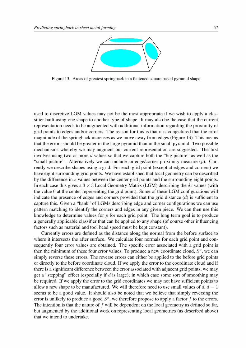
Predicting springback in sheet metal forming 57
Figure 13. Areas of greatest springback in a flattened square based pyramid shape
used to discretize LGM values may not be the most appropriate if we wish to apply a clas-sifier built using one shape to another type of shape. It may also be the case that the currentrepresentation needs to be augmented with additional information regarding the proximity ofgrid points to edges and/or corners. The reason for this is that it is conjectured that the errormagnitude of the springback increases as we move away from edges (Figure 13). This meansthat the errors should be greater in the large pyramid than in the small pyramid. Two possiblemechanisms whereby we may augment our current representation are suggested. The firstinvolves using two or more d values so that we capture both the “big picture” as well as the“small picture”. Alternatively we can include an edge/corner proximity measure (p). Cur-rently we describe shapes using a grid. For each grid point (except at edges and corners) wehave eight surrounding grid points. We have established that local geometry can be describedby the difference in z values between the center grid points and the surrounding eight points.In each case this gives a 3× 3 Local Geometry Matrix (LGM) describing the δz values (withthe value 0 at the center representing the grid point). Some of these LGM configurations willindicate the presence of edges and corners provided that the grid distance (d) is sufficient tocapture this. Given a “bank” of LGMs describing edge and corner configurations we can usepattern matching to identify the corners and edges in any given piece. We can then use thisknowledge to determine values for p for each grid point. The long term goal is to producea generally applicable classifier that can be applied to any shape (of course other influencingfactors such as material and tool head speed must be kept constant).
Currently errors are defined as the distance along the normal from the before surface towhere it intersects the after surface. We calculate four normals for each grid point and con-sequently four error values are obtained. The specific error associated with a grid point isthen the minimum of these four error values. To produce a new coordinate cloud, S ′′, we cansimply reverse these errors. The reverse errors can either be applied to the before grid pointsor directly to the before coordinate cloud. If we apply the error to the coordinate cloud and ifthere is a significant difference between the error associated with adjacent grid points, we mayget a “stepping” effect (especially if d is large); in which case some sort of smoothing maybe required. If we apply the error to the grid coordinates we may not have sufficient points toallow a new shape to be manufactured. We will therefore need to use small values of d, d = 1seems to be a good value. It should also be noted that we believe that simply reversing theerror is unlikely to produce a good S ′′, we therefore propose to apply a factor f to the errors.The intention is that the nature of f will be dependent on the local geometry as defined so far,but augmented by the additional work on representing local geometries (as described above)that we intend to undertake.
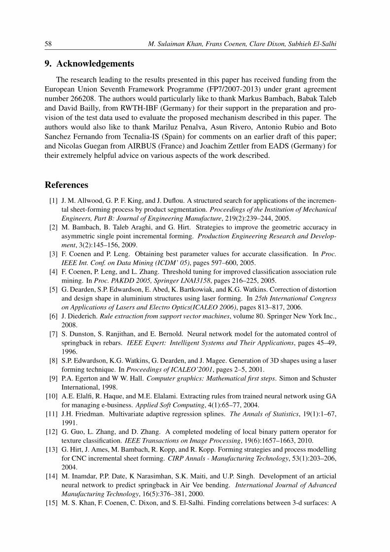
58 M. Sulaiman Khan, Frans Coenen, Clare Dixon, Subhieh El-Salhi
9. Acknowledgements
The research leading to the results presented in this paper has received funding from theEuropean Union Seventh Framework Programme (FP7/2007-2013) under grant agreementnumber 266208. The authors would particularly like to thank Markus Bambach, Babak Taleband David Bailly, from RWTH-IBF (Germany) for their support in the preparation and pro-vision of the test data used to evaluate the proposed mechanism described in this paper. Theauthors would also like to thank Mariluz Penalva, Asun Rivero, Antonio Rubio and BotoSanchez Fernando from Tecnalia-IS (Spain) for comments on an earlier draft of this paper;and Nicolas Guegan from AIRBUS (France) and Joachim Zettler from EADS (Germany) fortheir extremely helpful advice on various aspects of the work described.
References[1] J. M. Allwood, G. P. F. King, and J. Duflou. A structured search for applications of the incremen-
tal sheet-forming process by product segmentation. Proceedings of the Institution of MechanicalEngineers, Part B: Journal of Engineering Manufacture, 219(2):239–244, 2005.
[2] M. Bambach, B. Taleb Araghi, and G. Hirt. Strategies to improve the geometric accuracy inasymmetric single point incremental forming. Production Engineering Research and Develop-ment, 3(2):145–156, 2009.
[3] F. Coenen and P. Leng. Obtaining best parameter values for accurate classification. In Proc.IEEE Int. Conf. on Data Mining (ICDM’ 05), pages 597–600, 2005.
[4] F. Coenen, P. Leng, and L. Zhang. Threshold tuning for improved classification association rulemining. In Proc. PAKDD 2005, Springer LNAI3158, pages 216–225, 2005.
[5] G. Dearden, S.P. Edwardson, E. Abed, K. Bartkowiak, and K.G. Watkins. Correction of distortionand design shape in aluminium structures using laser forming. In 25th International Congresson Applications of Lasers and Electro Optics(ICALEO 2006), pages 813–817, 2006.
[6] J. Diederich. Rule extraction from support vector machines, volume 80. Springer New York Inc.,2008.
[7] S. Dunston, S. Ranjithan, and E. Bernold. Neural network model for the automated control ofspringback in rebars. IEEE Expert: Intelligent Systems and Their Applications, pages 45–49,1996.
[8] S.P. Edwardson, K.G. Watkins, G. Dearden, and J. Magee. Generation of 3D shapes using a laserforming technique. In Proceedings of ICALEO’2001, pages 2–5, 2001.
[9] P.A. Egerton and W W. Hall. Computer graphics: Mathematical first steps. Simon and SchusterInternational, 1998.
[10] A.E. Elalfi, R. Haque, and M.E. Elalami. Extracting rules from trained neural network using GAfor managing e-business. Applied Soft Computing, 4(1):65–77, 2004.
[11] J.H. Friedman. Multivariate adaptive regression splines. The Annals of Statistics, 19(1):1–67,1991.
[12] G. Guo, L. Zhang, and D. Zhang. A completed modeling of local binary pattern operator fortexture classification. IEEE Transactions on Image Processing, 19(6):1657–1663, 2010.
[13] G. Hirt, J. Ames, M. Bambach, R. Kopp, and R. Kopp. Forming strategies and process modellingfor CNC incremental sheet forming. CIRP Annals - Manufacturing Technology, 53(1):203–206,2004.
[14] M. Inamdar, P.P. Date, K Narasimhan, S.K. Maiti, and U.P. Singh. Development of an articialneural network to predict springback in Air Vee bending. International Journal of AdvancedManufacturing Technology, 16(5):376–381, 2000.
[15] M. S. Khan, F. Coenen, C. Dixon, and S. El-Salhi. Finding correlations between 3-d surfaces: A

Predicting springback in sheet metal forming 59
study in asymmetric incremental sheet forming. In Proc. Machine Learning and Data Mining inPattern Recognition (MLDM’12), Springer LNAI 7376, pages 336–379, 2012.
[16] D.J. Kim and B.M. Kim. Application of neural network and FEM for metal forming processes.International Journal of Machine Tools and Manufacture, 40(6):911–925, 1999.
[17] B. Kinsey, J. Cao, and S. Solla. Consistent and minimal springback using a stepped binderforce trajectory and neural network control. Journal of Engineering Materials and Technology,122(1113):113–118, 2000.
[18] W. Li, J. Han, and J. Pei. Cmar: Accurate and efficient classification based on multipleclass-association rules. In Proc. IEEE Int. Conf. on Data Mining (ICDM’ 05), pages 369–376,2001.
[19] K. Manabe, M. Yang, and S. Yoshihara. Artificial intelligence identification of process param-eters and adaptive control system for deep drawing process. Journal of Materials ProcessingTechnology, 80-81:421–426, 1998.
[20] N. Narasimhan and M. Lovell. Predicting springback in sheet metal forming an explicit to im-plicit sequential solution procedure. Finite Elements in Analysis and Design, 33(1):29–42, 1999.
[21] T. Ojala, M.P. Inen, and T. Maeenpae. Multiresolution gray-scale and rotation invariant textureclassification with local binary patterns. IEEE Transactions on Pattern Analysis and MachineIntelligence, 24(7):971–987, 2002.
[22] K.K. Pathak, S. Panthi, and N. Ramakrishnan. Application of neural network in sheet metalbending process. Defence Science Journal, 55(2):125–131, 2005.
[23] J. R. Quinlan. C4.5: programs for machine learning. Morgan Kaufmann Publishers Inc., 1993.[24] J.R. Quinlan. Induction of decision trees. Machine learning, 1(1):81–106, 1986.[25] R. Rufni and J. Cao. Using neural network for springback minimization in a channel forming
process. Journal of Materials and Manufacturing, 107(5):65–73, 1998.[26] J. Xu, Z. Zhang, and Y. Wu. Application of data mining method to improve the accuracy of
springback prediction in sheet metal forming. Journal of Shanghai University (English Edition),8(3):348–353, 2004.
[27] J.L. Yin and D.Y. Li. Knowledge discovery from finite element simulation data. In Proceedings of2004 International Conference on Machine Learning and Cybernetics, pages 1335–1340, 2004.
[28] X. Yin and J. Han. Cpar: Classification based on predictive association rules. In SIAM Int. Conf.on Data Mining (SDM’03), pages 331–335, 2003.
[29] S. Zhang, C. Luo, Y.H. Peng, D.Y. Li, and H.B. Yang. Study on factors affecting springbackand application of data mining in springback analysis. Journal of Shanghai Jiaotong University,E-8(2):192–196, 2003.
Journal of Theoretical and Applied Computer Science Vol. 6, No. 2, 2012, pp. 60–71ISSN 2299-2634 http://www.jtacs.org
Auto-kernel using multilayer perceptron
Wei-Chen ChengInstitute of Statistical Science, Academia Sinica, Taiwan, Republic of [email protected]
Abstract: This work presents a constructive method to train the multilayer perceptron layer after layer suc-cessively and to accomplish the kernel used in the support vector machine. Data in differentclasses will be trained to map to distant points in each layer. This will ease the mapping of thenext layer. A perfect mapping kernel can be accomplished successively. Those distant mappedpoints can be discriminated easily by a single perceptron.
Keywords: kernel function, support vector machine, multilayer perceptron
1. Introduction
The Mercer kernel function [15] has been widely used to map the data and informationonto another space, so that the data can be processed, used and manipulated in that space.The target space could have higher, lower, or even infinite dimension. In that space, onecan perform classification, principal component analysis, or clustering analysis to processthe data. The advantage is that the mapping provides the power of nonlinearity for thoselinear models to handle complex data. The mapped data can thus be applied to the traditionalanalysis algorithms. The class label of the data is not used in the design of the Mercer kernelfunction. There have been several developed Mercer kernel functions: polynomial kernel,sigmoid kernel, and Gaussian kernel using radial basis function. Those mappings have anattractive advantage that the inner product of the two mapped data can be efficiently calculatedfrom the original data with lower complexity. Therefore the trick is widely adopted and verypopular in practical applications to handle large-scale data and to accelerate the analysis.The trick has been applied to many linear models, like linear discriminative analysis [5],support vector machine [1], principal component analysis [16][18][4], and k-means. However,the trick relies on the form of inner product. In order to accelerate the computation of themapping, users have to choose one Mercer kernel function [15] among existing ones anddecide the parameters of the function, including the number of dimensions and the number ofpowers. The different settings of parameters will cause diverse results because the classifierand analyzer only process the mapped data without knowing the distribution of the data in theoriginal space. After the user chooses the Mercer kernel function, the inner cross-validationcan determine the parameters. The inner cross-validation is a process that divides the trainingdata into several chunks, uses parts of them to train the analyzer, and uses the remainingparts for validation. The process of the training and validation repeatedly tests all differentparameters thoroughly and the set of parameters which has the best result is selected. TheMercer kernel function with the set of parameters is then used for mapping all training dataonto the new space, so that the forthcoming and unseen data is analyzed in that space.
Auto-kernel using multilayer perceptron 61
The search for the parameters is in a discrete space and is independent to the analysisperformed at the mapped space. A convex property for the analyzer is therefore beneficialfor saving the computation power. The result of the mapping is nonlinear with respect to theparameters, and the nonlinearity causes difficulty for the users to perceive the outcome andhard to control the parameters by themselves.
In this work, we present a learnable mapping function and describe its learning algo-rithm [9, 10, 3, 11]. This auto-kernel function is applied to perform the task of SVM-likeclassification [1], which maximizes the margin of the separation boundary. The proposedkernel function is constructed by a MLP (multilayer perceptron) to separate data into differentclasses. Users need not to select from different types of function because the proposed kernelis capable of learning the mapping automatically. The only parameter which will affect theoutcome and has to be determined by user is the number of neurons. The number decides thepower of the auto-kernel function. The proposed classifier can be applied to multiple-classproblem.
2. Constructive auto-kernel functionWe have a dataset which consists of data patterns and labels. The pattern described here is
the training data used for constructing a model and has multiple dimensions, which are corre-sponding to the properties of that pattern. Let x denote the pattern, which is a n0-dimensionalcolumn vector and the collection of the pattern is X =
{x1,x2, . . . ,xP
}. The size of X
is the number of the pattern in the set, |X| = P . Set a label function, C : Rn0 → N,that maps each coordinate, x, to its class identification number (or class label), C (x). Thelabel is an integer from 1 to T . The pattern xp which is sampled from the space with certainprobability distribution is mapped to its label C (xp). All pairs of the patterns are classifiedinto different sets according to their labels. Let the set V contain pattern pairs that belongto the same class, V = {(xp,xq);C(xp) = C(xq)} and U contain the pairs that belongto different classes, U = {(xp,xq);C(xp) = C(xq)} . In order to minimize the risk [19],the separation boundary should be at the position that maximizes the margin of separationplane. The distance between the plane and the closest points is maximized. The networkfor implementing the mapping function has L layers. The output vector of all neurons in mthlayer is a column vector and is also the internal representation y(p,m). The superscript p meansthe input pattern is xp as well as the input layer, y(p,0) = xp. The number of neurons in themth layer is denoted by nm. The collection of all internal representations of the mth layer isYm =
{y(1,m),y(2,m), . . . ,y(P,m)
}. The representations may be the same, y(p,m) = y(q,m),
for different patterns xp = xq. They are treated to be the same when the distance betweenthem is close to zero,
∥∥y(p,m) − y(q,m)∥∥ < ϵ. This mapping is a many-to-one mapping. Set
|Ym| is to be the number of distinct representations in the set Ym. All patterns have theirinternal representations in each layer, which are the output vectors of the layers. The inter-nal representations are studied in [13]. The representations, y(p,m), are binary codes whilethe hard-limit activation function is adopted. The hyperplane of each neuron divides its in-put space, which is from the previous layer, into two partitions. All hyperplanes in a layerdivide their input space into non-overlapping decision areas, hence each area has a binarycode. The decision area has a polyhedral shape and each of the codes y(p,m) represents thepatterns in one decision area. According to the study of [13], the number of significant rep-resentations will be reduced significantly layer after layer. A significant representation meansthere exists a pattern with that representation. The mathematical expression is expressed as

62 Wei-Chen Cheng∣∣YL∣∣ ≪ . . . ≪ |Y2| ≪ |Y1| ≪ P . We expect the number of significant representation
will converge to the number of classes,∣∣YL
∣∣ = T . This makes the design possible for theauto-learning kernel function.
The upper bound of the number of neurons in the mth layer is⌈∥Ym−1∥nm−1
⌉≥ nm for
solving a general-position two-class classification problem [12]. For the number of neuronsin the first hidden layer, n1, the bound is
⌈Pn0
⌉≥ n1. With this weight design, the reduced
number in the last layer L is guaranteed,∣∣YL
∣∣ = T .The “AIR” tree [13] can be used for detecting the faulty representations of the patterns
in the hidden layer. The erroneous neurons result from that the confused patterns of twoclasses have the same code. Consequently, a single code y(p,m) = y(q,m) represents patternsin different classes, (xp,xq) ∈ U . The study shows that any back-propagation algorithmcannot correct such latent errors by adjusting the synapse weights in its succeeding layers thatnear the output layer. The front layers must be trained correctly so that their succeeding layerscan receive proper signals. In the light of this, the MLP has to be accomplished layer by layer.A bottom-up construction is hence proposed.
The mechanism of the back-propagation training [17] of the front layers has further beenstudied [13]. The main mechanism is the categorization of data pattern into different classesand therefore the value of class label is not applicable in the categorization. The study suggestsan objective function that trains the front layers successfully by using the differences betweenclasses.
The SIR (Separable Internal Representation) method in [9] provides such objective func-tion based on the differences between classes. The network can be trained layer after layerusing this objective function starting from the first hidden layer. Perfect categorization andproduction of correct signals can be accomplished for each layer [9][10]. These front layersare served, suitably, as the auto-kernel function. The auto-kernel will utilize the differencesbetween classes to train the front layers, and it will not use the class label information in itstraining process. The idea is expressed in Figure 1.
Besides the front layer, the mechanism of rear layers which are near the output layer hasalso been identified [13]. The main mechanism is the labeling. The cooperation of the frontand rear layers complete the supervised MLP. We will include a labeling sector that containsseveral layers after the auto-kernel. The outputs of the objective function for the labelingsector are the class labels. The nL-dimensional output vector of the auto-kernel function isconverted to the class label, where the C (x) dimension is 1 and all the other dimensionsare −1.
Figure 1. The idea of the implementation of neural lens
We will use the differences between classes to train each front layer starting from the firsthidden layer. A second hidden layer is added to the first hidden layer when the outputs ofthe first hidden layer cannot produce correct isolated signals for each class. However, when a

Auto-kernel using multilayer perceptron 63
hidden layer does produce correct isolated signals, it will be served as the last front layer, L,and as the output of the kernel. We expect that the number of reduced representations of thelast front layer will equal to the number of classes,
∣∣YL∣∣ = T .
3. Learning algorithm for auto-kernel functionFigure 2 shows the auto-kernel function and the labeling sector. This function consists of
layered neurons. For a pair of patterns in the same class, (xp,xq) ∈ V , the synapse weightsof each layer are adjusted by using the energy function [10],
Eatt (xp,xq) =1
2
∥∥y(p,m) − y(q,m)∥∥2
, (1)
to reduce the distance between their output vectors,∥∥y(p,m) − y(q,m)
∥∥. However, for differentclasses, (xp,xq) ∈ U , the weights are adjusted by using the energy function,
Erep (xp,xq) =−12
∥∥y(p,m) − y(q,m)∥∥2
, (2)
to increase the distance between their output vectors. The difference between classes is implic-itly used in two energies. Note that the value of the class label is not used in these two objectivefunctions. The value of the labels will be applied only in the labeling sector. The magnitude ofthe energy functions (1) and (2) are 0 ≤ Eatt (xp,xq) ≤ 2nm and−2nm ≤ Erep (xp,xq) ≤ 0.The value of (1) converges toward zero from 2nm. The value of (2) comes close to −2nm
from zero.The network is constructed layer after layer, starting from L = 1. A new hidden layer
is added, Lnew=Lold + 1, whenever Lold layers cannot accomplish the isolation. All synapseweights of the trained layers are fixed during the training of that additional layer, m = Lold+1.
The synaptic weight matrix which connects the output of the (m− 1)th layer and theinput of the mth layer, is denoted by Wm. The W1 connects the input layer and the firsthidden layer. Applying the gradient descent method to the added layer, the two energies canbe reduced efficiently during the training stage. The successfully trained network is used asthe auto-kernel function to map out the pattern, xp, in the output space, y(p,L).
Suppose there are two classes, C (x) ∈ {1, 2}. The training algorithm is as follows:
1. For the added layer Wm (Wm from W1 to WL)2. For limited epochs3. Pick two patterns in the same class, xp1 and xp2 , which satisfy the following
condition(xp1 ,xp2) = argmax
{(xi,xj)∈V }
∥∥y(i,m) − y(j,m)∥∥2
. (3)
Among all pairs of patterns in the same class, the two patterns (xp1 ,xp2) have the longestdistance in the output space of the mth layer.
4. Find the pair of patterns, xq1 and xq2 in different classes, which satisfy
(xq1 ,xq2) = argmin{(xi,xj)∈U}
∥∥y(i,m) − y(j,m)∥∥2
. (4)
The pair of patterns (xq1 ,xq2) have the shortest distance in the output space of the mthlayer.
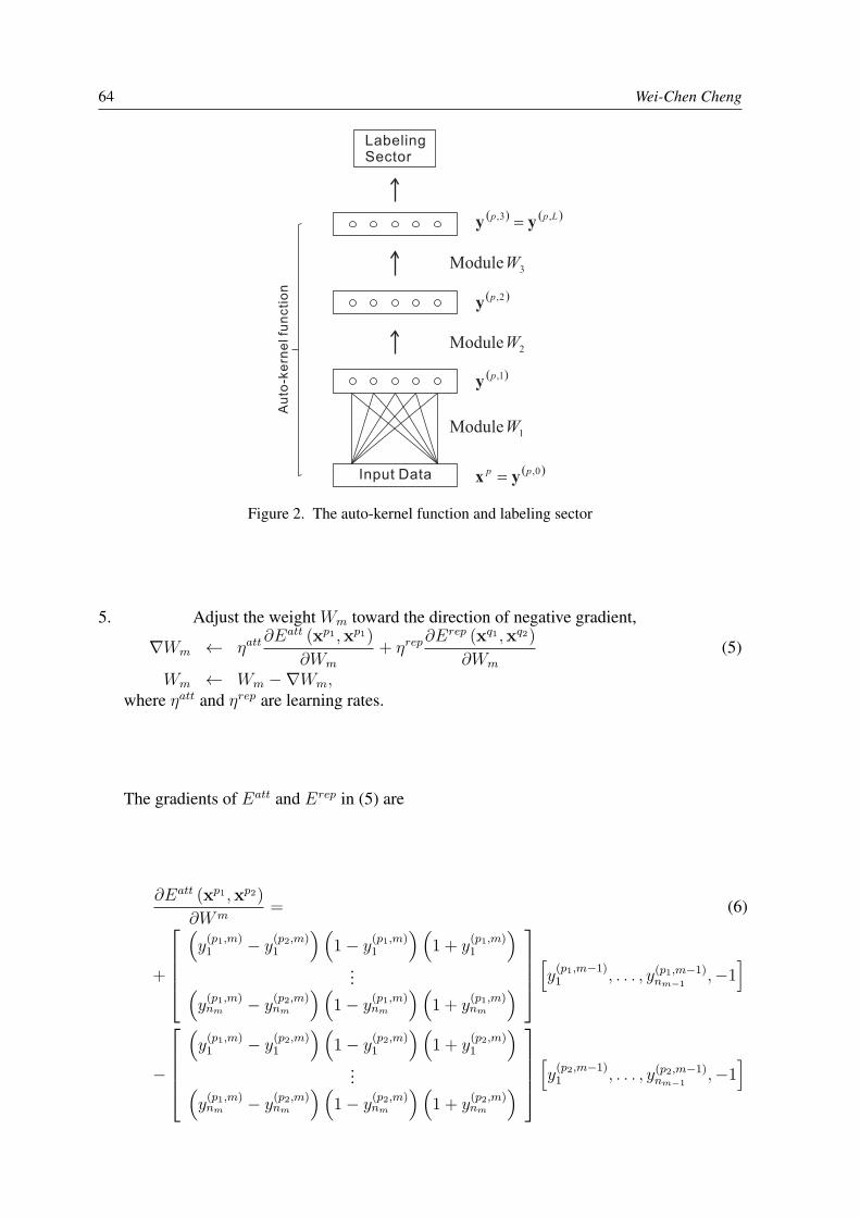
64 Wei-Chen Cheng
Figure 2. The auto-kernel function and labeling sector
5. Adjust the weight Wm toward the direction of negative gradient,
∇Wm ← ηatt∂Eatt (xp1 ,xp1)
∂Wm
+ ηrep∂Erep (xq1 ,xq2)
∂Wm
(5)
Wm ← Wm −∇Wm,where ηatt and ηrep are learning rates.
The gradients of Eatt and Erep in (5) are
∂Eatt (xp1 ,xp2)
∂Wm= (6)
+
(y(p1,m)1 − y
(p2,m)1
)(1− y
(p1,m)1
)(1 + y
(p1,m)1
)...(
y(p1,m)nm − y
(p2,m)nm
)(1− y
(p1,m)nm
)(1 + y
(p1,m)nm
)[
y(p1,m−1)1 , . . . , y(p1,m−1)
nm−1,−1
]
−
(y(p1,m)1 − y
(p2,m)1
)(1− y
(p2,m)1
)(1 + y
(p2,m)1
)...(
y(p1,m)nm − y
(p2,m)nm
)(1− y
(p2,m)nm
)(1 + y
(p2,m)nm
)[
y(p2,m−1)1 , . . . , y(p2,m−1)
nm−1,−1
]
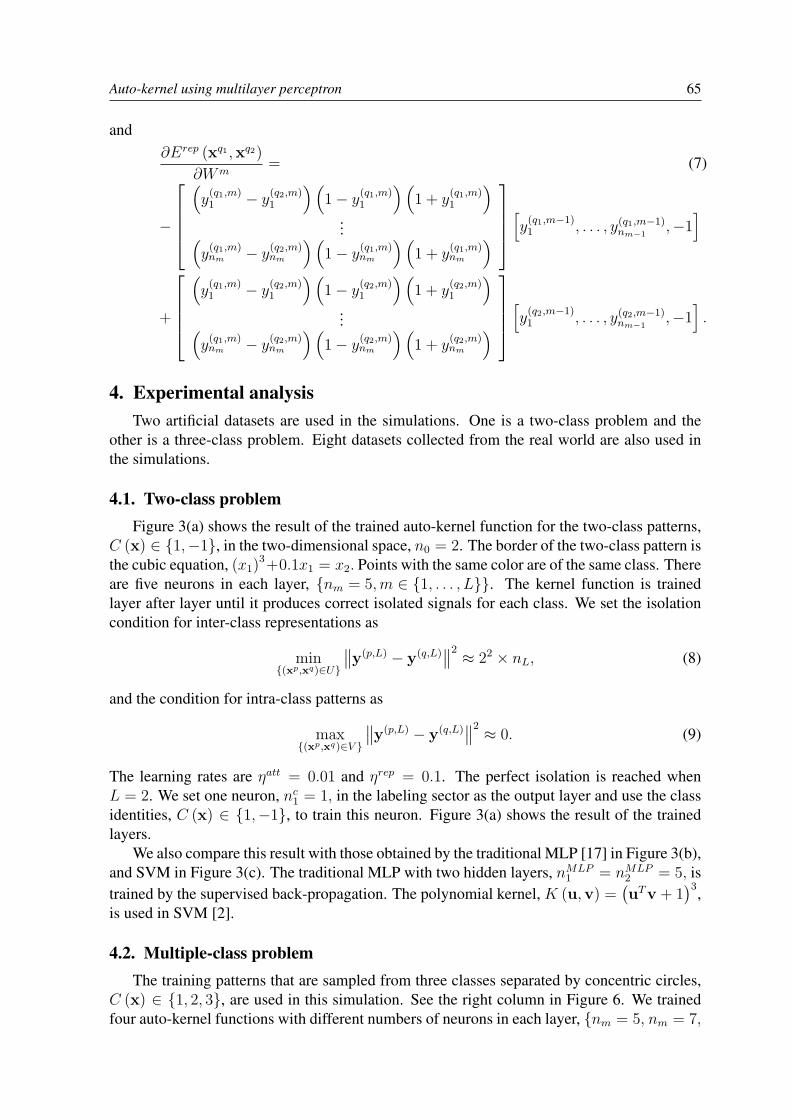
Auto-kernel using multilayer perceptron 65
and∂Erep (xq1 ,xq2)
∂Wm= (7)
−
(y(q1,m)1 − y
(q2,m)1
)(1− y
(q1,m)1
)(1 + y
(q1,m)1
)...(
y(q1,m)nm − y
(q2,m)nm
)(1− y
(q1,m)nm
)(1 + y
(q1,m)nm
)[
y(q1,m−1)1 , . . . , y(q1,m−1)
nm−1,−1
]
+
(y(q1,m)1 − y
(q2,m)1
)(1− y
(q2,m)1
)(1 + y
(q2,m)1
)...(
y(q1,m)nm − y
(q2,m)nm
)(1− y
(q2,m)nm
)(1 + y
(q2,m)nm
)[
y(q2,m−1)1 , . . . , y(q2,m−1)
nm−1,−1
].
4. Experimental analysisTwo artificial datasets are used in the simulations. One is a two-class problem and the
other is a three-class problem. Eight datasets collected from the real world are also used inthe simulations.
4.1. Two-class problemFigure 3(a) shows the result of the trained auto-kernel function for the two-class patterns,
C (x) ∈ {1,−1}, in the two-dimensional space, n0 = 2. The border of the two-class pattern isthe cubic equation, (x1)
3+0.1x1 = x2. Points with the same color are of the same class. Thereare five neurons in each layer, {nm = 5,m ∈ {1, . . . , L}}. The kernel function is trainedlayer after layer until it produces correct isolated signals for each class. We set the isolationcondition for inter-class representations as
min{(xp,xq)∈U}
∥∥y(p,L) − y(q,L)∥∥2 ≈ 22 × nL, (8)
and the condition for intra-class patterns as
max{(xp,xq)∈V }
∥∥y(p,L) − y(q,L)∥∥2 ≈ 0. (9)
The learning rates are ηatt = 0.01 and ηrep = 0.1. The perfect isolation is reached whenL = 2. We set one neuron, nc
1 = 1, in the labeling sector as the output layer and use the classidentities, C (x) ∈ {1,−1}, to train this neuron. Figure 3(a) shows the result of the trainedlayers.
We also compare this result with those obtained by the traditional MLP [17] in Figure 3(b),and SVM in Figure 3(c). The traditional MLP with two hidden layers, nMLP
1 = nMLP2 = 5, is
trained by the supervised back-propagation. The polynomial kernel, K (u,v) =(uTv + 1
)3,is used in SVM [2].
4.2. Multiple-class problemThe training patterns that are sampled from three classes separated by concentric circles,
C (x) ∈ {1, 2, 3}, are used in this simulation. See the right column in Figure 6. We trainedfour auto-kernel functions with different numbers of neurons in each layer, {nm = 5, nm = 7,
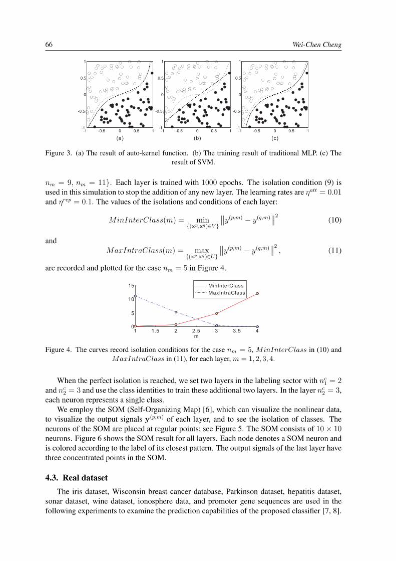
66 Wei-Chen Cheng
Figure 3. (a) The result of auto-kernel function. (b) The training result of traditional MLP. (c) Theresult of SVM.
nm = 9, nm = 11}. Each layer is trained with 1000 epochs. The isolation condition (9) isused in this simulation to stop the addition of any new layer. The learning rates are ηatt = 0.01and ηrep = 0.1. The values of the isolations and conditions of each layer:
MinInterClass(m) = min{(xp,xq)∈V }
∥∥y(p,m) − y(q,m)∥∥2
(10)
andMaxIntraClass(m) = max
{(xp,xq)∈U}
∥∥y(p,m) − y(q,m)∥∥2
, (11)
are recorded and plotted for the case nm = 5 in Figure 4.
Figure 4. The curves record isolation conditions for the case nm = 5, MinInterClass in (10) andMaxIntraClass in (11), for each layer, m = 1, 2, 3, 4.
When the perfect isolation is reached, we set two layers in the labeling sector with nc1 = 2
and nc2 = 3 and use the class identities to train these additional two layers. In the layer nc
2 = 3,each neuron represents a single class.
We employ the SOM (Self-Organizing Map) [6], which can visualize the nonlinear data,to visualize the output signals y(p,m) of each layer, and to see the isolation of classes. Theneurons of the SOM are placed at regular points; see Figure 5. The SOM consists of 10× 10neurons. Figure 6 shows the SOM result for all layers. Each node denotes a SOM neuron andis colored according to the label of its closest pattern. The output signals of the last layer havethree concentrated points in the SOM.
4.3. Real datasetThe iris dataset, Wisconsin breast cancer database, Parkinson dataset, hepatitis dataset,
sonar dataset, wine dataset, ionosphere data, and promoter gene sequences are used in thefollowing experiments to examine the prediction capabilities of the proposed classifier [7, 8].
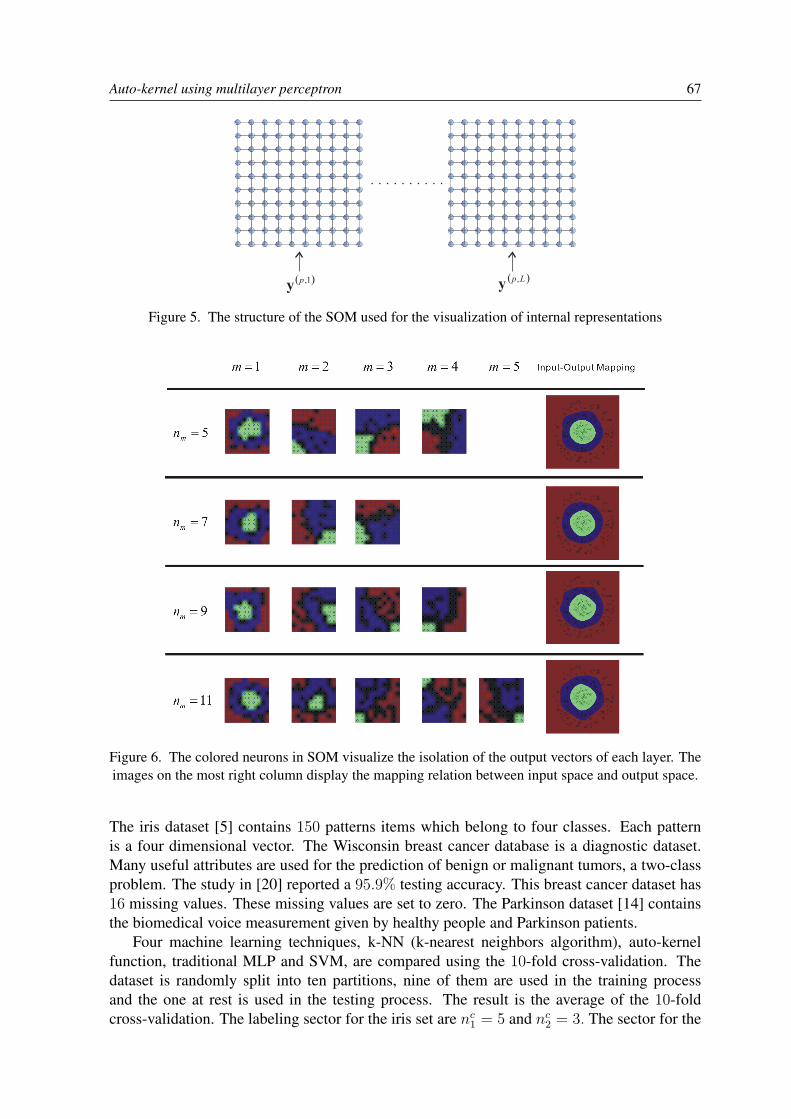
Auto-kernel using multilayer perceptron 67
Figure 5. The structure of the SOM used for the visualization of internal representations
Figure 6. The colored neurons in SOM visualize the isolation of the output vectors of each layer. Theimages on the most right column display the mapping relation between input space and output space.
The iris dataset [5] contains 150 patterns items which belong to four classes. Each patternis a four dimensional vector. The Wisconsin breast cancer database is a diagnostic dataset.Many useful attributes are used for the prediction of benign or malignant tumors, a two-classproblem. The study in [20] reported a 95.9% testing accuracy. This breast cancer dataset has16 missing values. These missing values are set to zero. The Parkinson dataset [14] containsthe biomedical voice measurement given by healthy people and Parkinson patients.
Four machine learning techniques, k-NN (k-nearest neighbors algorithm), auto-kernelfunction, traditional MLP and SVM, are compared using the 10-fold cross-validation. Thedataset is randomly split into ten partitions, nine of them are used in the training processand the one at rest is used in the testing process. The result is the average of the 10-foldcross-validation. The labeling sector for the iris set are nc
1 = 5 and nc2 = 3. The sector for the
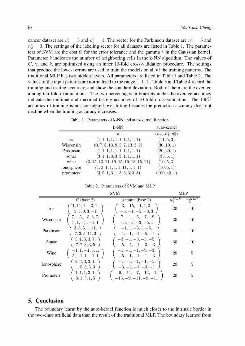
68 Wei-Chen Cheng
cancer dataset are nc1 = 5 and nc
2 = 1. The sector for the Parkinson dataset are nc1 = 5 and
nc2 = 3. The settings of the labeling sector for all datasets are listed in Table 1. The parame-
ters of SVM are the cost C for the error tolerance and the gamma γ in the Gaussian kernel.Parameter k indicates the number of neighboring cells in the k-NN algorithm. The values ofC, γ, and k, are optimized using an inner 10-fold cross-validation procedure. The settingsthat produce the lowest errors are used to train the models on all of the training patterns. Thetraditional MLP has two hidden layers. All parameters are listed in Table 1 and Table 2. Thevalues of the input patterns are normalized to the range [−1, 1]. Table 3 and Table 4 record thetraining and testing accuracy, and show the standard deviation. Both of them are the averageamong ten-fold examinations. The two percentages in brackets under the average accuracyindicate the minimal and maximal testing accuracy of 10-fold cross-validation. The 100%accuracy of training is not considered over-fitting because the prediction accuracy does notdecline when the training accuracy increases.
Table 1. Parameters of k-NN and auto-kernel function
k-NN auto-kernelk (nm, nc
1, nc2)
iris (1, 1, 1, 1, 1, 1, 1, 1, 1, 1) (11, 5, 3)Wisconsin (3, 7, 5, 13, 9, 5, 7, 13, 3, 5) (30, 10, 1)Parkinson (1, 1, 1, 1, 1, 1, 1, 1, 1, 1) (20, 20, 1)
sonar (3, 1, 1, 3, 3, 3, 1, 1, 1, 1) (35, 5, 1)wine (3, 15, 13, 11, 19, 15, 19, 13, 15, 11) (10, 5, 3)
ionosphere (1, 3, 1, 1, 1, 1, 11, 1, 1, 1) (10, 5, 1)promoters (3, 5, 1, 3, 1, 3, 3, 3, 3, 3) (100, 40, 1)
Table 2. Parameters of SVM and MLP
SVM MLPC (base 2) gamma (base 2) nMLP
1 nMLP2
iris(
1, 11, 1,−3, 1,5, 5, 9, 3,−1
) (3,−15,−1, 1, 3,−5,−1,−5,−3, 3
)20 10
Wisconsin(
7,−5,−5, 3, 7,3, 1,−3,−1, 1
) (−7,−1,−5,−7,−9,−3,−5,−3,−5, 1
)30 10
Parkinson(
3, 3, 5, 1, 11,7, 3, 5, 11, 3
) (−1, 1,−3, 1,−5,−1,−1,−1,−5,−1
)20 10
Sonar(
5, 1, 5, 3, 7,7, 7, 3, 3, 5
) (−3,−1,−3,−3,−5,−5,−5,−1,−3,−3
)30 10
Wine(−1, 1,−1, 3, 1,5,−1, 1,−1, 1
) (−1,−1,−1,−9,−3,−5,−1,−1,−1,−3
)20 5
Ionosphere(
3, 3, 3, 3, 1,1, 5, 3, 5, 3
) (−1,−1,−1,−1,−5,−3,−5,−1,−3,−1
)20 5
Promoters(
1, 1, 1, 3, 1,5, 1, 3, 1, 5
) (−9,−11,−7,−13,−7,−15,−9,−11,−9,−11
)20 5
5. ConclusionThe boundary learnt by the auto-kernel function is much closer to the intrinsic border in
the two-class artificial data than the result of the traditional MLP. The boundary learned from
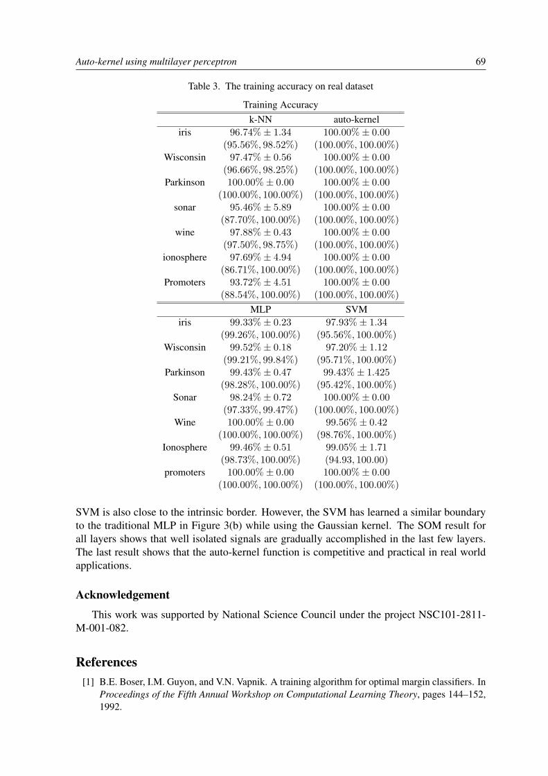
Auto-kernel using multilayer perceptron 69
Table 3. The training accuracy on real dataset
Training Accuracyk-NN auto-kernel
iris 96.74%± 1.34 100.00%± 0.00(95.56%, 98.52%) (100.00%, 100.00%)
Wisconsin 97.47%± 0.56 100.00%± 0.00(96.66%, 98.25%) (100.00%, 100.00%)
Parkinson 100.00%± 0.00 100.00%± 0.00(100.00%, 100.00%) (100.00%, 100.00%)
sonar 95.46%± 5.89 100.00%± 0.00(87.70%, 100.00%) (100.00%, 100.00%)
wine 97.88%± 0.43 100.00%± 0.00(97.50%, 98.75%) (100.00%, 100.00%)
ionosphere 97.69%± 4.94 100.00%± 0.00(86.71%, 100.00%) (100.00%, 100.00%)
Promoters 93.72%± 4.51 100.00%± 0.00(88.54%, 100.00%) (100.00%, 100.00%)
MLP SVMiris 99.33%± 0.23 97.93%± 1.34
(99.26%, 100.00%) (95.56%, 100.00%)Wisconsin 99.52%± 0.18 97.20%± 1.12
(99.21%, 99.84%) (95.71%, 100.00%)Parkinson 99.43%± 0.47 99.43%± 1.425
(98.28%, 100.00%) (95.42%, 100.00%)Sonar 98.24%± 0.72 100.00%± 0.00
(97.33%, 99.47%) (100.00%, 100.00%)Wine 100.00%± 0.00 99.56%± 0.42
(100.00%, 100.00%) (98.76%, 100.00%)Ionosphere 99.46%± 0.51 99.05%± 1.71
(98.73%, 100.00%) (94.93, 100.00)promoters 100.00%± 0.00 100.00%± 0.00
(100.00%, 100.00%) (100.00%, 100.00%)
SVM is also close to the intrinsic border. However, the SVM has learned a similar boundaryto the traditional MLP in Figure 3(b) while using the Gaussian kernel. The SOM result forall layers shows that well isolated signals are gradually accomplished in the last few layers.The last result shows that the auto-kernel function is competitive and practical in real worldapplications.
Acknowledgement
This work was supported by National Science Council under the project NSC101-2811-M-001-082.
References[1] B.E. Boser, I.M. Guyon, and V.N. Vapnik. A training algorithm for optimal margin classifiers. In
Proceedings of the Fifth Annual Workshop on Computational Learning Theory, pages 144–152,1992.
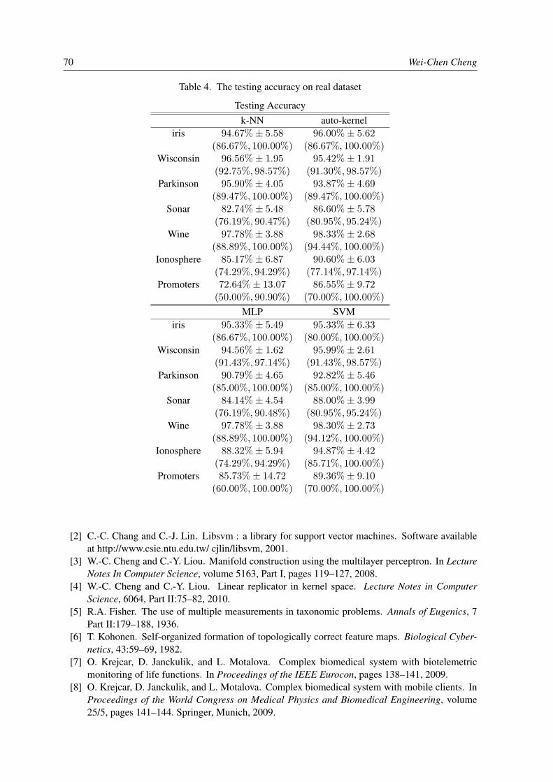
70 Wei-Chen Cheng
Table 4. The testing accuracy on real dataset
Testing Accuracyk-NN auto-kernel
iris 94.67%± 5.58 96.00%± 5.62(86.67%, 100.00%) (86.67%, 100.00%)
Wisconsin 96.56%± 1.95 95.42%± 1.91(92.75%, 98.57%) (91.30%, 98.57%)
Parkinson 95.90%± 4.05 93.87%± 4.69(89.47%, 100.00%) (89.47%, 100.00%)
Sonar 82.74%± 5.48 86.60%± 5.78(76.19%, 90.47%) (80.95%, 95.24%)
Wine 97.78%± 3.88 98.33%± 2.68(88.89%, 100.00%) (94.44%, 100.00%)
Ionosphere 85.17%± 6.87 90.60%± 6.03(74.29%, 94.29%) (77.14%, 97.14%)
Promoters 72.64%± 13.07 86.55%± 9.72(50.00%, 90.90%) (70.00%, 100.00%)
MLP SVMiris 95.33%± 5.49 95.33%± 6.33
(86.67%, 100.00%) (80.00%, 100.00%)Wisconsin 94.56%± 1.62 95.99%± 2.61
(91.43%, 97.14%) (91.43%, 98.57%)Parkinson 90.79%± 4.65 92.82%± 5.46
(85.00%, 100.00%) (85.00%, 100.00%)Sonar 84.14%± 4.54 88.00%± 3.99
(76.19%, 90.48%) (80.95%, 95.24%)Wine 97.78%± 3.88 98.30%± 2.73
(88.89%, 100.00%) (94.12%, 100.00%)Ionosphere 88.32%± 5.94 94.87%± 4.42
(74.29%, 94.29%) (85.71%, 100.00%)Promoters 85.73%± 14.72 89.36%± 9.10
(60.00%, 100.00%) (70.00%, 100.00%)
[2] C.-C. Chang and C.-J. Lin. Libsvm : a library for support vector machines. Software availableat http://www.csie.ntu.edu.tw/ cjlin/libsvm, 2001.
[3] W.-C. Cheng and C.-Y. Liou. Manifold construction using the multilayer perceptron. In LectureNotes In Computer Science, volume 5163, Part I, pages 119–127, 2008.
[4] W.-C. Cheng and C.-Y. Liou. Linear replicator in kernel space. Lecture Notes in ComputerScience, 6064, Part II:75–82, 2010.
[5] R.A. Fisher. The use of multiple measurements in taxonomic problems. Annals of Eugenics, 7Part II:179–188, 1936.
[6] T. Kohonen. Self-organized formation of topologically correct feature maps. Biological Cyber-netics, 43:59–69, 1982.
[7] O. Krejcar, D. Janckulik, and L. Motalova. Complex biomedical system with biotelemetricmonitoring of life functions. In Proceedings of the IEEE Eurocon, pages 138–141, 2009.
[8] O. Krejcar, D. Janckulik, and L. Motalova. Complex biomedical system with mobile clients. InProceedings of the World Congress on Medical Physics and Biomedical Engineering, volume25/5, pages 141–144. Springer, Munich, 2009.

Auto-kernel using multilayer perceptron 71
[9] C.-Y. Liou, H.-T. Chen, and J.-C. Huang. Separation of internal representations of the hiddenlayer. In Proceedings of the 2000 International Computer Symposium, pages 26–34, 2000.
[10] C.-Y. Liou and W.-C. Cheng. Resolving hidden representations. In Lecture Notes in ComputerScience, volume 4985, Part II, pages 254–263. Springer, Heidelberg, 2008.
[11] C.-Y. Liou and W.-C. Cheng. Forced accretion and assimilation based on self-organizing neuralnetwork. In Self Organizing Maps - Applications and Novel Algorithm Design, pages 683–702,2011.
[12] C.-Y. Liou and W.-J. Yu. Initializing the weights in multilayer network with quadratic sigmoidfunction. In Proceedings of the International Conference on Neural Information Processing,pages 1387–1392, 1994.
[13] C.-Y. Liou and W.-J. Yu. Ambiguous binary representation in multilayer neural network. InProceedings of International Conference on Neural Networks, volume 1, pages 379–384, 1995.
[14] M.A. Little, P.E. McSharry, S.J. Roberts, D.A.E. Costello, and I.M. Moroz. Exploiting nonlinearrecurrence and fractal scaling properties for voice disorder detection. BioMedical EngineeringOnLine, 6:23, 2007.
[15] J. Mercer. Functions of positive and negative type and their connection with the theory of integralequations. Philosophical Transactions of the Royal Society A, 209:415V446, 1909.
[16] L. Pearson. On lines and planes of closest fit to systems of points in space. PhilosophicalMagazine, 2(11):559–572, 1901.
[17] D.E. Rumelhart, G.E. Hinton, and R.J. Williams. Learning internal representations by errorpropagation. In Parallel Distributed Processing: Explorations in the Microstructure of Cogni-tion, volume 1, pages 318–362. Cambridge, MA: MIT Press, 1986.
[18] Bernhard Scholkopf, Alexander Smola, and Klaus-Robert Muller. Nonlinear component analysisas a kernel eigenvalue problem. Psychometrika, 10:1299–1319, 1998.
[19] Vladimir Vapnik. The nature of statistical learning theory. In Information Science and Statistics,2000.
[20] W.H. Wolberg and O.L. Mangasarian. Multisurface method of pattern separation for medicaldiagnosis applied to breast cytology. In Proceedings of the National Academy of Sciences, vol-ume 87, pages 9193–9196, 1990.
Journal of Theoretical and Applied Computer Science Vol. 6, No. 2, 2012, pp. 72–78ISSN 2299-2634 http://www.jtacs.org
Artistic ideation based on computer vision methods
Ferran Reverter, Pilar Rosado, Eva Figueras, Miquel Angel PlanasUniversity of Barcelona, Spain{freverter,efigueras}@ub.edu, {prrforma,miquelplanas}@gmail.com
Abstract: This paper analyzes the automatic classification of scenes that are the basis of the ideation andthe designing of the sculptural production of an artist. The main purpose is to evaluate the per-formance of the Bag-of-Features methods, in the challenging task of categorizing scenes whenscenes differ in semantics rather than the objects they contain. We have employed a kernel-basedrecognition method that works by computing rough geometric correspondence on a global scaleusing the pyramid matching scheme introduced by Lazebnik [7]. Results are promising, on averagethe score is about 70%. Experiments suggest that the automatic categorization of images basedon computer vision methods can provide objective principles in cataloging images.
Keywords: bag-of-features, SIFT descriptors, pyramid match kernel, artistic ideation
1. IntroductionImage representation is a very important element for image classification, annotation, seg-
mentation or retrieval. Nearly all the methods in computer vision which deals with imagecontent representation resort to features capable of representing image content in a compactway. Local features based representation can produce a versatile and robust image representa-tion capable of representing global and local content at the same time. Describing an object orscene using local features computed at interest locations makes the description robust to par-tial occlusion and image transformation. This results from the local character of the featuresand their invariance to image transformations.
The bag-of-visterms (BOV) is an image representation built from automatically extractedand quantized local descriptors referred to as visterms in the remainder of this paper. TheBOV representation, which is derived from these local features, has been shown to be one ofthe best image representations in several tasks.
The main objective of this study is assessing the performance of SIFT descriptors, BOVrepresentation and spatial pyramid matching for automatic analysis of images that are thebasis of the ideation and designing of art work. Additionally, we explore the capability of thiskind of modelization to become useful for the production of software based art.
2. Image Representation and MatchingThe BOV representation was first used [1] as an image representation for an object recog-
nition system. In the BOV representation, local descriptors fj are quantized into their respec-tive visterms vi = Q(fj) and used to represent the images from which they were extracted.The quantization process groups similar descriptors together, with the aim that the descriptorsin each resulting group arises from local patterns with similar visual appearance. The number
Artistic ideation based on computer vision methods 73
of occurrences of each visterm in a given image is the elementary feature of the BOV repre-sentation. More precisely, the BOV representation is the histogram of the various visterms’occurrences.
To construct the BOV feature vector h from an image I four steps are required. In brief, lo-cal interest points are automatically detected in the image, then local descriptors are computedover the regions defined around those local interest points (certain applications may requirethat local descriptors may be computed on a dense grid over the image instead over localinterest points). After this extraction step, the descriptors are quantized into visterms, and alloccurrences of each visterm of the vocabulary are counted to build the BOV representation ofthe image.
2.1. Feature extractionThe BOV construction requires two main design decisions: the choice of local descriptors
that we apply on our images to extract local features, and the choice of which method we useto obtain the visterms’ vocabulary. Both of these choices can influence the resulting system’sperformance. Nevertheless BOV is a robust image representation, which retains its goodperformance over a large range of parameter choices.
For better discriminative power, we utilize higher dimensional features which are SIFT(Scale Invariant Feature Transform) descriptors introduced by [2]. The SIFT descriptor is ahistogram based representation of the gradient orientations of the gray-scale image patch. Inour study, SIFT descriptors are computed at points on a regular grid with spacing 8 pixels.At each grid point the descriptors are computed over circular support patches. Our decisionto use a dense regular grid instead of interest points was based on the comparative evaluationof [3], who have shown that dense features work better for scene classification. Intuitively, adense image description is necessary to capture uniform regions such as sky, calm water, orroad surface. SIFT was also found to work best for the task of object classification [4] and[5].
2.2. Visual VocabularyIn order to obtain a text-like representation, we quantize each local descriptor s into one
of a discrete set V of visterms v according to a nearest neighbor rule:
s 7→ Q(s) = vi ↔ dist(s, vi) ≤ dist(s, vj),
for all j = 1, ...,M , where M denotes the size of the visterm set.We will call vocabulary the set V of all the visterms. The vocabulary construction is
performed through clustering. More specifically, we apply the k-means algorithm to a set oflocal descriptors extracted from training images, and keep the means as visterms. We usedthe Euclidean distance in the clustering and quantization processes, and choose the number ofclusters depending on the desired vocabulary size.
Finally, the BOV representation is constructed from local descriptors according to:
h(d) =(n(d, v1), n(d, v2), ..., n(d, vM)
)with n(d, vi), i = 1, ...,M , denotes the number of occurrences of visterm vi in image d. Toclassify an input image d represented either by the bag-of-visterms vector h(d) we employedSupport Vector Machines (SVMs).

74 Ferran Reverter, Pilar Rosado, Eva Figueras, Miquel Angel Planas
This vector-space representation of an image contains no information about spatial rela-tionships between visterms, in the same way the standard bag-of-words text representationremoves the word ordering information.
For such whole-image categorization tasks, bag-of-features methods, which representsan image as an orderless collection of local features, have recently demonstrated impressivelevels of performance. However, because these methods disregard all information about thespatial layout of the features, they have severely limited descriptive ability. In particular, theyare incapable of capturing shape or of segmenting an object from its background.
2.3. Spatial matching scheme
To overcome the limitations of the bag-of-visterms approach, a spatial pyramid matchingscheme was introduced in [8] and [7]. Informally, pyramid matching works by placing asequence of increasingly coarser grids over the feature space and taking a weighted sum ofthe number of matches that occur at each level of resolution. At any fixed resolution, twopoints are said to match if they fall into the same cell of the grid; matches found at finerresolutions are weighted more heavily than matches found at coarser resolutions.
More specifically, let X and Y be two sets of vectors in a p-dimensional feature space. Letus construct a sequence of grids at resolutions 0, ..., L such that the grid at level ℓ has 2ℓ cellsalong each dimension, for a total of D = 2pℓ cells. Let Hℓ
X and HℓY denote the histograms of
X and Y at this resolution, so that HℓX(i) and Hℓ
Y (i) are the numbers of points from X andY that fall into the ith cell of the grid. Then the number of matches at level ℓ is given by thehistogram intersection function:
I(HℓX , H
ℓY ) =
D∑i=1
min(Hℓ
X(i), HℓY (i)
).
With the aim of brevity, we will abbreviate I(HℓX , H
ℓY ) = Iℓ. Note that the number of
matches found at level ℓ also includes all the matches found at the finer level ℓ+1. Therefore,the number of new matches found at level ℓ is given by Iℓ − Iℓ+1 for ℓ = 0, ..., L − 1. Theweight associated with level ℓ is set to 1
2L−ℓ , which is inversely proportional to cell width atthat level. Intuitively, we want to penalize matches found in larger cells because they involveincreasingly dissimilar features.
Putting all the pieces together, the pyramid match kernel [8] is defined by
κL(X, Y ) =1
2LI0 +
∑ℓ=1
L1
2L−ℓ+1Iℓ.
As introduced in [8], a pyramid match kernel works with an orderless image represen-tation. It allows for precise matching of two collections of features in a high dimensionalappearance space, but discards all spatial information.
Lazebnik et all. [7] advocates an approach that has the advantage of maintaining conti-nuity with the popular ”visual vocabulary” paradigm. It performs pyramid matching in thetwo-dimensional image space, and uses traditional clustering techniques in feature space.
Specifically, we quantize all feature vectors into a set of M discrete types, visual terms,and make the simplifying assumption that only features of the same type can be matched toone another.

Artistic ideation based on computer vision methods 75
Each channel m gives us two sets of two-dimensional vectors, Xm and Ym, representingthe coordinates of features of type m found in the respective images. The final kernel is thenthe sum of the separate channel kernels:
KL(X, Y ) =M∑
m=1
κL(Xm, Ym). (1)
This approach agrees with Bag-of-visterms, in fact, it reduces to a standard bag of featureswhen L = 0.
Because the pyramid match kernel is simply a weighted sum of histogram intersections,and because cmin(a, b) = min(ca, cb) for positive numbers, we can implement (1) as a singlehistogram intersection of ”long” vectors formed by concatenating the appropriately weightedhistograms of all channels at all resolutions. For L levels and M channels, the resulting vectorhas dimensionality M
∑Lℓ 4
l = M 13(4L+1 − 1).
In summary, both the histogram intersection and the pyramid match kernel are Mercerkernels [8]. Lazebnik et all. [7] extend the pyramid match kernel to the pyramid of histogramof visual terms. Bosch et al. [6] implement a pyramid of histograms of visual terms, inspiredin the above spatial matching scheme, but using a gaussian like kernel. In this implementationthe similarity between a pair of images I and J is computed using a kernel function betweentheir pyramid of histograms of visual terms DI and DJ , with appropriate weighting for eachlevel of the pyramid:
K(DI , DJ) = exp{ 1β
∑l∈L
αldl(DI , DJ)}
where β is the average of∑
l∈L αldl(DI , DJ) over the training data, αl is the weight at whichlevel l and dl is the χ2 distance [9] between DI and DJ at pyramid level l computed using thenormalized histograms at that level.
Spatial histograms could be used as image descriptors and fed to a linear SVM classifier.Linear SVMs are very fast to train, but also limited to use an inner product to compare de-scriptors. Vedaldi and Fulkerson [10] have shown that much better results can be obtained bycomputing an explicit feature map that emulates a non linear χ2-kernel as a linear one.
3. ResultsIn this paper we propose to automatically analyze images from a database of photographs
by Dr. M.A. Planas Rossello (Professor of sculpture, University of Barcelona). The imageresolution is 480 × 480. The database consists of 150 images previously classified in 5 cate-gories: Central architecture (CA), Geometric stone (GS), Irregular stone (IS), Textured stone(TS) and Silhouettes (SI). These categories correspond to 5 different typologies identified inthe photographic images from the database. Images are the basis for the ideation and designof an artist’s sculptural work.
Figure 1 schematizes the steps in image analysis using a pyramid of histograms of visualterms. A dense grid of points is defined on the image, then local descriptors are computed overthe regions defined around those points in the grid. After this extraction step, the descriptorsare quantized into visual terms (visterms). Then, the image is represented by visterms, each
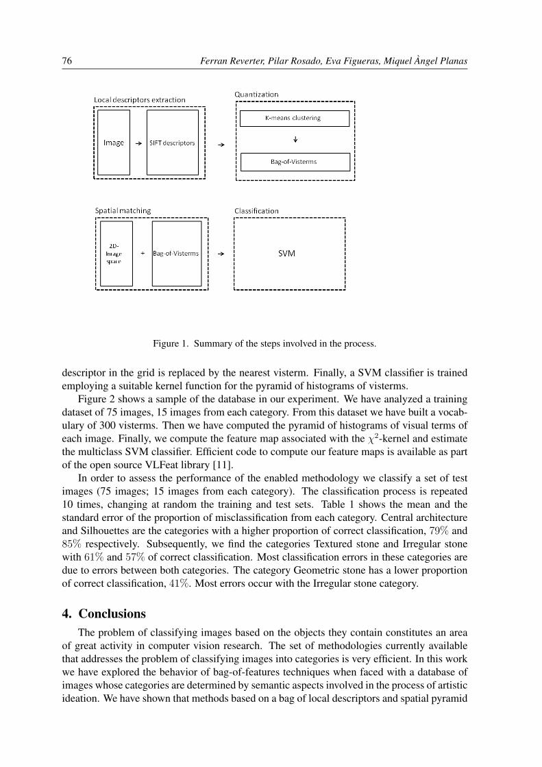
76 Ferran Reverter, Pilar Rosado, Eva Figueras, Miquel Angel Planas
Figure 1. Summary of the steps involved in the process.
descriptor in the grid is replaced by the nearest visterm. Finally, a SVM classifier is trainedemploying a suitable kernel function for the pyramid of histograms of visterms.
Figure 2 shows a sample of the database in our experiment. We have analyzed a trainingdataset of 75 images, 15 images from each category. From this dataset we have built a vocab-ulary of 300 visterms. Then we have computed the pyramid of histograms of visual terms ofeach image. Finally, we compute the feature map associated with the χ2-kernel and estimatethe multiclass SVM classifier. Efficient code to compute our feature maps is available as partof the open source VLFeat library [11].
In order to assess the performance of the enabled methodology we classify a set of testimages (75 images; 15 images from each category). The classification process is repeated10 times, changing at random the training and test sets. Table 1 shows the mean and thestandard error of the proportion of misclassification from each category. Central architectureand Silhouettes are the categories with a higher proportion of correct classification, 79% and85% respectively. Subsequently, we find the categories Textured stone and Irregular stonewith 61% and 57% of correct classification. Most classification errors in these categories aredue to errors between both categories. The category Geometric stone has a lower proportionof correct classification, 41%. Most errors occur with the Irregular stone category.
4. ConclusionsThe problem of classifying images based on the objects they contain constitutes an area
of great activity in computer vision research. The set of methodologies currently availablethat addresses the problem of classifying images into categories is very efficient. In this workwe have explored the behavior of bag-of-features techniques when faced with a database ofimages whose categories are determined by semantic aspects involved in the process of artisticideation. We have shown that methods based on a bag of local descriptors and spatial pyramid

Artistic ideation based on computer vision methods 77
CA GS IS SI TSCA 0.79(0.04) 0(0) 0.04(0.003) 0.17(0.03) 0.01(0.007)GS 0.14(0.02) 0.41(0.04) 0.31(0.05) 0.11(0.011) 0.03(0.011)IS 0.01(0.01) 0.19(0.04) 0.57(0.02) 0(0) 0.23(0.011)SI 0.11(0.01) 0.01(0.01) 0(0) 0.85(0.014) 0.03(0.011)TS 0(0) 0.01(0.01) 0.37(0.011) 0(0) 0.61(0.017)
Table 1. True category in rows and Predicted category in columns. Categories are: Central architecture(CA), Geometric stone (GS), Irregular stone (IS), Silhouettes (SI) and Textured stone (TS). Cells in the
table show the mean and the standard error, in brackets, of the proportion of misclassification.
Figure 2. A sample from the dataset of images.
matching are adequate for the classification of images whose categories are based on semanticaspects. Experiments suggest that the automatic categorization of images based on computervision methods can provide objective principles in cataloging images.
5. AcknowledgementsWe would like to thank two anonymous reviewers for helpful comments on the manuscript.
This work was partially funded by the University of Barcelona grant APPCSHUM 2011-2012.
References[1] Willamowski, J., Arregui, D., Csurka, G., Dance, C- and Fan, L. 2004. Categorizing nine vi-
sual classes using local appearance descriptors. Proceedings of LAVS Workshop, in ICPR’04.Cambridge.
[2] Lowe, D. G. 2004 Distinctive image features from scale-invariant keypoints. International Jour-nal of Computer Vision 60(2),91:110.

78 Ferran Reverter, Pilar Rosado, Eva Figueras, Miquel Angel Planas
[3] Fei-Fei, L and Perona, P. 2005. A Bayesian hierarchical model for learning natural scene cate-gories. In Proceedings of CVPR.
[4] Sivic, J., Russell, B. C., Efros, A. A., Zisserman, A., and Freeman, W. T. 2005. Discoveringobjects and their location in image collections. In Proceedings of IEEE International Conferenceon Computer Vision, Beijing.
[5] Quelhas, P., Monay, F., Odobez, J.-M., Gatica-Perez, D., Tuytelaars, T., and Gool, L. V. 2005.Modeling scenes with local descriptors and latent aspects. In Proceedings of IEEE InternationalConference on Computer Vision (ICCV), Beijing.
[6] Bosch, A., Zisserman, A., Munoz, X. 2007. Image Classification using Random Forests andFerns. In Proceedings of IEEE International Conference on Computer Vision (ICCV).
[7] Lazebnik, S., Schmid, C., and Ponce, J. 2006. Beyond bags of features: Spatial pyramid matchingfor recognizing natural scene categories. In Proceedings of CVPR.
[8] Grauman, K. and Darrel, T. 2005. The pyramid match kernel: Discriminative classification withsets of image features. In Proceedings of IEEE International Conference on Computer Vision(ICCV), Beijing.
[9] Zhang,J., Marszaek,M., Lazebnik, C., and Schmid, S. 2007. Local features and kernels for clas-sification of texture and object categories: a comprehensive study. International Journal of Com-puter Vision. DOI: 10.1007/s11263-006-9794-4.
[10] Vedaldi, A.,and Zisserman, A. 2010. Efficient Additive Kernels via Explicit Feature Maps. InProceedings of CVPR.
[11] Vedaldi, A., and Fulkerson, B. 2008. VLFeat library (http://www.vlfeat.org/).


Related Documents