Classical Noise. VI. Noise in Self-Sustained Oscillators near Threshold

PHYSICAL REVIEW VOLUME 161,. NUMBER 2 10 SEPTEMBER 1967

Classical Noise. VI. Noise in Self-Sustained Oscillators nearThreshold. *

RoBERT D. HEMPSTEADt AND MELvIN LAxBell Telephone Laboratories, ItIz~rray Hil/, New Jersey

(Received 28 March 1967)

Because of the relative narrowness of the threshold region, a general model for spectrally pure self-sustained oscillators (both classical and quantum, including gas lasers) can be reduced, in the thresholdregion, to a rotating-wave Van der Pol (RWVP) oscillator. By a scaling transformation, we reduce to thenormalized RWVP oscillator which contains only one dimensionless parameter, a net pump rate p, whichdetermines the operating point. The power spectra of phase and amplitude fluctuations and of amplitude(intensity) fluctuations in the normalized RWVP oscillator near threshold are calculated "exactly" bynumerical Fokker-Planck methods. Using the appropriate scaling transformation, our results yield thesepower spectra for any oscillator of this general type. In particular, for gas lasers our results yield the one-sided Fourier transform of (bt(t)b(0) ) (the spectrum) and of (b t(0) b(tt) b(t)b(0) )—(b"b)' (the intensityspectrum), where bt and b are the creation and destruction operators for the radiation field. Except forintensity fluctuations just above threshold, the power spectra were found to be nearly Lorentzian, withhalf-widths at half power approximately equal to the lowest nonzero temporal eigenvalue of the Fokker-Planck equation. For intensity Quctuations above threshold, the second-lowest nonzero eigenvalue wasfound to yield a significant contribution to the power spectrum as well as the lowest nonzero eigenvalue.These two eigenvalues become nearly degenerate for operation well above threshold. Thus the intensityfluctuation spectrum is Lorentzian below and well above threshold, but more complex in the thresholdregion.

1. INTRODUCTION

~

CONSIDERABLE attention has been given recently~ to the Van der Pol oscillator as a semiclassical

way of describing noise in masers and lasers. ' It hasbeen shown for the gas laser, and any other laser forwhich the atomic rate constants are fast compared tothe photon-decay constants, that the electromagnetic-Geld operators have a Markman behavior and obey"Heisenberg" equations of the rotating-wave Van derPol form" (RWVP) with quantum-noise sources thatcan be calculated from Grst principles. 4

~ The work reported here overlaps appreciably the contents ofa thesis submitted by R. D. H. to the Department of ElectricalEngineering, Massachusetts Institute of Technology in September1965, in partial fulfillment of the requirements for a Master ofScience degree. Part of this work was previously presented at theNew York meeting of the American Physical Society, Bull. Am.Phys. Soc. 11, 111 (1966).

f Present address: Physics Department, University of Illinois,Urbana, Illinois.' The importance of Van der Pol oscillators in describing lasersand laser noise has been emphasized by a number of authors:W. Lamb, Jr., Phys. Rev. 134, A1429 (1964); H. A. Haus, J.Quant. Electron. 1, 179 (1965); C. Freed and H. A. Haus, Appl.Phys. Letters 6, 85 (1965); Phys. Rev. 141, 287 (1966); J. A.Armstrong and A. W. Smith, Phys. Rev. Letters 14, 68, 208(1965); Phys. Letters 16, 38 (1965); Phys. Rev. 140, A155(1965);H. Risken, Z. Physik 191, 302 (1966).' M. Lax and W. H. Louisell, J. Quant. Electron. 3, 47 (1967).hereafter referred to as QIX (see Ref. 3).

s QIX stands for the ninth paper in a series of papers on quan-tum noise by M. Lax: QI: Phys. Rev. 109, 1921 (1958); QII:129, 2342 (1963); QIII: J. Phys. Chem. Solids 25, 487 (1964);QIV: Phys. Rev. 145, 110 (1966); QV: in Physics of QuantumElectronics, edited by P. L. Kelley, B. Lax, and P. E. Tannen-wald (McGraw-Hill Book Company, Inc. , New York, 1966)p. 735; QVI: (with D. R. Fredkin) (to be published); QVII:J. Quant. Electron. 3, 37 (1967); QVIII: H. Cheng and M. Laxin QNantum Theory of the Solid State, edited by Per-Olav Lowdin(Academic Press Inc. , New York, 1966), p. 587; QIX: (withW. H. Louisell), J. Quant. Electron. 3, 47 (1967); QX: Phys.Rev. 157, 213 (1967); QXI: (to be published); QXII: with W.H. Louisell (to be pubhshed),

~ See QIV.

With the exception of the density-matrix treatmentof Scully, Stephen and Lamb, ' previous treatmentshave made quantum-mechanical calculations of diffu-sion coefFicients and inserted them into a classicalFokker-Planck equation. ' Even then, quasilinear ap-proximations' have usually been used to avoid thesolution of the Fokker-Planck equations that consti-tute the exact description of the classical random proc-esses. For operation near the threshold of oscillation,quasilinear approximations are not valid, and one isforced to solve the Fokker-Planck equation.

Two different linearization schemes have been incommon use. The mean-value method, ' as explainedin V, deals with the real and imaginary parts of theGeM as variables and replaces a nonlinear resistanceby a mean value. For a laser, the population differenceis not treated as a fluctuating variable, but replacedby a mean value. ' In V, we suggested that this methodshould be adequate well below threshold, since the

s M. Scully, W. E. Lamb, Jr. , and M. J. Stephen, in Physics ofQNantum Electronics, edited by P. L. Kej.ley, B. Lax, and P. E.Tannenwald (McGraw-Hill Book Company, Inc. , New York,1966),p. 759; M. Scully and W. E. Lamb, Jr., Phys. Rev. Letters16, 853 (1966).

'H. Haken, Z. Physik 190, 327 (1966); H. Sauermann, ibid.188, 480 (1965); 189, 312 (1966);H. Risken, C. Schmid, and W.Weidlich, Phys. Letters 20, 489 (1966).' For a general discussion of quasilinear methods see I; for aquasilinear treatment of seH-sustained oscillators see V, the firstand fifth papers in the series on classica] noise by M. Lax: I:Rev. Mod. Phys. 32, 25 (1960); II: J. Phys. Chem. Solids 14,248 (1960); III: Rev. Mod. Phys. 38, 359 (1966); IV: 38, 541(1966); V: Bull. Am. Phys. Soc. 11, 111 (1966) and Phys. Rev.160, 290 (1967).

'W. G. Wagner and G. Birnbaum, J. Appl. Phys. 32, 1185(1961); D. E. McCumber, Phys. Rev. 130, 675 (1962); A. L.Schawlow and C. H. Townes, ibid. 112, 1940 (1958);J. A. Fleck,Jr., J. Appl. Phys. 34, 2997 (1963); R. V. Pound, Ann. Phys.(N. Y.) 1, 24 (1957); M. P. W. Strandberg, Phys. Rev. 106, 617(1957);J. Weber, Rev. Mod. Phys. 31, 681 (1959);K. H. Wells,Ann. Phys. (N. Y.) 12, 1 (1961);G. Kemeny, Phys. Rev, 133,A69 (1964); H. Risken, Z. Physik 180, 150 (1964).350

CLAS SICAL NO IS E. VI 351

nonlinear term, although crudely treated, is small com-pared to the linear term which then is dominant indetermining the over-all response. The second lineariza-tion scheme' used the amplitude and phase of the fieldvariables, and makes a quasilinear approximation inthe amplitude only. This method used, for example,by the Haken School, ' and by us' in QV, was recog-nized' in V to be valid only well above threshold.

The present paper supplies exact numerical solutionsof the Fokker-Planck equation. In the region nearthreshold, (power output within a factor of 10 of thethreshold value), we demonstrate that neither lineariza-tion scheme is sufFiciently accurate. We also demon-strate our previous conjectures that the mean-valuemethod is adequate well below threshold, and that thequasilinear method becomes increasingly accurate wellabove threshold. These qualitative conclusions are alsosuggested by Risken's" variational treatment of thelowest eigenfunctions of the Fokker-Planck operator.

The spectrum of our oscillator (for a laser, this isthe Fourier transform of (bt(t) b(0) ), where bt and b

are creation and destruction operators for the harmonicoscillator describing the field) is shown to be nearlyLorentzian. Thus the linewidth of this noise spectrumwill be determined, as demonstrated below, primarilyby the lowest eigenvalue h~ (tb for phase) of the Fokker-Planck operator for the restricted set of eigenfunctionswhich vary as exp(ip), that determine the spectrumof phase @ (and amplitude r=

~ls

~ ) fluctuations con-tained in (r(t) expLig(t)]r(0) expL —ip(0) j).

As is well known, the linewidth A„ is inversely pro-portional to the power. The proportionality constantobtained by the mean-value method (see for examplethe Schawlow-Townes' formula) is twice that obtainedby the quasilinear method. ' Our present numerical re-sults for A„display the transition from the Schawlow-Townes formula, below threshold, to the quasilinearformula above threshold.

The spectrum of intensity (pure amplitude) fluctua-tions )for a laser this is the Fourier transform of(bt(0) bt (t) b(t) b(0) )] is also demonstrated to be nearlyLorentzian except for a region just above threshold. Inthe Lorentzian region, the linewidth is determined bythe lowest nonvanishing eigenvalue A, for the phase-independent solutions of the Fokker-Planck equation.The quasilinear estimate of this linewidth, as well as A,display a minimum near threshold in agreement withexperimental measurements of amplitude fluctuations. "

See for example, W. A. Edson, Proc. IRE 48, 1454 (1960);J. A. Mullen, ibid. 48, 1467 (1960); M. E. Golay, ibid. 48, 1473(1960};P. Grivet and A. Blaquiere, in Optical Physics (JohnWiley R Sons, Inc. , New York, 1963), p. 69. See also the manyrelevant papers in P. I. Kuznetsov, R. I. Stratanovitch, and V.I. Tikhonov, Non-Linear Transformations of Stochastic Processes(Pergamon Press, Oxford, England 1965).

'o H. Risken, Z. Physik 191, 302 (1966)."C.Freed and H. A. Haus, Phys. Rev. 141, 287 {1966);J. A.

Armstrong and A. W. Smith, ibid. 140, A155 (1965); F. T.Arecchi, Phys. Rev. Letters 15, 912 (1965); F. T. Arecchi, A.Berne, and P. Bulamacchi, ibid. 16, 32 (1966); W. Martienssenand F. Spiller, Phys. Rev. 145, 285 (1966).See also Ref. 1.

The basis for our ability to apply the results of aclassical random problem to the laser, which is a quan-tum random problem, is given in QIX' by Lax andLouisell, who have set up a dynamical correspondencebetween the density matrix of the electromagneticfield p(b, bt, t) and an associated classical functionp" (p, p*, t)."The correspondence is simply that thedensity operator is to be obtained from its associatedclassical function by replacing P by ls and P* by bt

obeying the antinormal ordering rule: all b~'s are to beplaced to the right, and all b's are to be placed to theleft. The classical average of any classical function3f&"'(p, p*, t) of p and p* over the classical probabilitydistribution pt'&(p, p*, t) corresponds to the quarttutttaverage of the quantum operator M(b, bt, t) obtainedfrom M&"'(P, P*, t) by replacing P by b and P* by bt

and obeying the normal ordering rule: All bt's are tobe placed to the left, and all li's are to be placed to theright. (The relation between our ordering procedureand the classical correspondences, adopted by otherauthors are discussed, " "with references, in QIX andQX.)

In QXII, Lax and Louisell obtain a Fokker —Planckequation for p'i(P, P*, 1Vt, 1V&, t) where 1V, and 1V s arepopulations of the lower and upper laser levels, respec-tively. "For a laser in which all of the atomic responserates are fast compared to the photon rates, an adia-batic approximation for the population variables E~ and1Vs yields a Fokker-Planck equation for p&'(P, P*, t).In Appendix A we quote the Langevin process appro-priate to this Fokker-Planck process. Treatment of thenonlinearity by an expansion in

~ p ~

is shown in Ap-pendix A (a) to lead to the Van der Pol oscillator,(b) to be valid from zero photons up to a number ofphotons greatly exceeding the number at threshold.

In Appendix 8 we consider a classical circuit modelof an oscillator to demonstrate that the reduction to

» We have established in QIX that, at any one time, our "classi-cal" function p&'& (p, p~, t) is identical {aside from a factor s.) tothe P(P} function of Glauber (see Ref. 13), Sudarshan (seeRef. 14) and Klauder (see Ref. 15). Our procedure is dynamicalin that we calculate P(P, t) using a Fokker-Planck equation de-scription of the field plus reservoirs rather than using a conjec-tured steady state P(P) plus free field dynamics (Refs. 13-15).A demonstration of the full equivalence between averages oftime-ordered, normally-ordered operators in the quantum prob-lem and ordinary averages in the associated "classical" problemis established in QXI. See also M. Lax, in Brartdess Sgmmer Irsstitute in Theoretica/ Physics Lecture Notes (Gordon and Breach,Science Publishers, Inc. , New York, to be published}, Chap. 11.

'3 R. J. Glauber, Phys. Rev. 130, 2529 (1963);131,2766 (1963).'4E. C. G. Sudarshan, Phys. Rev. Letters 10, 277 (1963);

Proceedings of the Symposium on Optical &users (John Wiley andSons, Inc. , New York 1963), p. 45.

» See also J. R. Klauder, J. Math. Phys. 4, 1055 (1963); 5,177, 878 (1964) and Phys. Rev. Letters 16, 534 (1966'). For anexcellent review, see L. Mandel and E. Wolf, Rev. Mod. Phys.37, 231 (1965).

'6 See also M. Lax, in Dynamical Processes in Solid State Optics(W. A. Benjamin Tnc. , New York, 1967},p. 195. A descriptionin terms of the field, NI, and N2 is appropriate when the popula-tion equilibration times are comparable (or slower) than thoseof the field. If NI empties rapidly, a simpler description in termsof p(b, bt, fVs, t) is possible as shown in QX.

R D. HEM P STEAD AND M. LAX 161

Van der Pol form over a broad region including thresh-old is valid for nearly all "well-designed" oscillators.We define a well-designed oscillator to be one whose

output is sinusoidal rather than periodic, and whose

output is large compared to thermal noise in a similarcircuit in which all resistances are positive.

In Appendices A and 3, we show that it is possibleto scale our amplitude variable and the time in sucha way as to eliminate all parameters but a singledimensionless parameter p. For a laser, P is propor-tional to the excess of the pump rate over the threshold

pump rate. Our scaled Langevin equations are justthose of the normalized rotating wave Van der Pol(NRWVP) oscillator equations studied in V r by quasi-linear methods.

We can, therefore, for a broad class of oscillatorsstart with the NRWVP-oscillator Langevin equations.The corresponding Fokker-Planck equation is derivedusing the real and imaginary parts of the complex

amplitude of the oscillator as variables. Since we areinterested in phase and amplitude noise, a transforma-tion to the magnitude and phase of the complex ampli-tude is made in Sec. 3. In order to reduce the numberof variables in the Fokker-Planck equation, certainintegrals over the phase variable are performed sinceit is only these integrals over the probability distribu-tion which are needed. In Sec. 5 we obtain the steady-state amplitude probability distribution, which is usedto obtain the dependence of the scaled photon number(or scaled intensity) p on our dimensionless pumpparameter p. By taking the one-sided Fourier trans-form of the equation resulting from the phase integralsover the Fokker-Planck equation, we obtain an ordimary

differential equation for a Green's function whose mo-ments give directly the power spectra of phase andamplitude fluctuations and of amplitude (intensity)

fluctuations.

This linear differential equation was numericallyintegrated and the power spectra for operation nearthreshold were obtained. Appendix C is a discussionof the boundary conditions used in this numerical inte-gration.

These power spectra were found to be very nearlyLorentzian for frequencies less than, and of the orderof, the half-width at half power. This suggested theusefulness of the usual expansion' of the conditionalprobability distribution in the eigenfunctions corre-sponding to the temporal eigenvalues of the Fokker-Planck equation, since a nearly Lorentzian power spec-trum ixnplies that the contribution of the lowest non-zero eigenvalue is dominant. The half-widths at halfpower of these power spectra were found to be given

by the lowest nonzero eigenvalues. We compare theexact results to what has been called an intelligentquasilinear approximation in V.

We want to emphasize that our exact results need

2. THE LANGEVIN AND FOKKER-PLANCKEQUATIONS

Our remarks of the preceding section establish the ap-propriateness of beginning with the "reduced" Langevinequations for the normalized rotating-wave Van der Poloscillator, V LEq. (9.4) j.'r

dh/dt = [p (x'+y') ]x+—F,(t),

dy/dt =Lp—(x'+y') jy+&, (t),

(2.1)

(2.2)

where the Langevin forces P, and P„represent Gaussianwhite-noise sources with the following moments:

(P,&= (P„)=0,

only be scaled by the scaling factors given in AppendixA to give the results for a gas laser, and by the scalingfactors in Appendix 8 to give the results for a largeclass of oscillators.

The present work divers from that of previous au-

thors in the following respects:

(1) From the direct correspondence between thedensity matrix and a classical probability distributionestablished in QIX, the quantum mec-ltanicat spectrumand moments are precisely calculated in terms of thecorresponding classical spectra and moments.

(2) All results and figures shown here were obtained

by numerical integration of the appropriate Fokker-Planck equations and are esseeti atty exact.

(3) A direct calculation is made of the power spectraof phase and amplitude Quctuations and of amplitude(intensity) fiuctuations by Green's-function methods.

(4) The results are checked by eigenfunction meth-ods. For this latter purpose, numerical computationswere made of the ten lowest nonzero eigenvalues andtheir corresponding eigenfunctions. This was done bothfor the usual spectrum (phase and amplitude fluctua-

tions) and for intensity fluctuations for values of Pcovering the threshold region. Risken'e estimated (byvariational methods only) the lowest eigenvalues Ao

A, in these two series.(5) The Scully-Lamb procedure~ (even if they per-

formed a time scaling) would retain two parameterssince the discrete photon number e cannot be scaledwithout approximation. Our scaling down to a singleparameter p permits numerical solution of differentialequations exploring a one-dimensional parameter space.The Scully-Lamb procedure, as presently used, mustperform the much greater labor of exploring a two-

parameter space. Moreover, for each point in thatspace, they solve not a single second-order diGerentialequation but an X)&X system of simultaneous equa-tions where T must be large compared to the meannumber of photons.

"See M. Lax, in Brandeis Summer Institute ~e TheoreticalPhysics Lectlre Notes (Gordon and Breach Science PublishersInc., Neer York, to be published). (2.3)

&61 CLASSICAL N0 I S E. VI

Since these Langevin forces are assumed Gaussian"

(Fi(fi) ~ ~ F„(t„)&z=0 for n) 2; (2.4)

where ( )~ denotes a linked average"" and F;(t;) =F.(f,) or F„(f;).

Because our noise sources are white, this process isMarkoffian and therefore the conditional probabilityP(x, y, t

~xp yp, fp) obeys a generalized Fokker-Planck

equation LIV(5.13)g:

()P co—= 2 (—1)"(~/~a) ":LD-(a, f) P(a, f) 1, (2 5)Bt

where a=a~, a2 ~ are the set of random variables —inthis case x and y—and the diffusion coeKcients D„aredefined by

I!D„(a,t)

= pm (at)-' f p(a', tpd((a, t) (a' —a) "sa', (2.|pAt~0

where D„has ss (suppressed) subscripts, and: is a short-hand notation which tells us to multiply correspondingterms, e.g. , the moment of (ui' —ai)'(as' —as) would bewritten Bi~2 and the corresponding term in the Fokker-Planck equation would be ( —1) (8'/8'ai())as) LDiisP).The m=1 and m=2 terms correspond to the ordinaryFokker-Planck equation, and the Gaussian propertyof our Langevin forces guarantees that all higher-orderdiffusion coefFicients for our process vanish. "

To obtain the first- and second-order diffusion coefB-cients, "we must write the Langevin equations as inte-gral equations:

ax=x(f+af) —x(f)t+b, t

I LP p(s)]x(s)+F (s) }ds (2 ")t

where p(s) =—t x(s) ]'+Ly(s) $' and similarly for hy. We

now iterate these integral equations by first replacingx(s), and y(s) inside the integral by x(t) and y(t),respectively, yielding the first approximation:

t+LL t

(Ax) =Pp p(t) jx(t) At+— F,(s) ds (2.8)t

and similarly for (hy) i.

From the definition of the diffusion coeS.cients D„,Eq. (2.6), we see that hx and Ay need be calculatedto only first order in ht. Care must be exercised, how-ever, since means of products of the Langevin forcesare singular, hence nominally higher-order terms maycontain a contribution which is 6.rst order in At. Toresolve this question, we must examine

t+/est t+d t t+b, t

dSy ' ' d$22g dSy ' ' dSt t t

X(F*( )" F.(-)F.( ')" F.( ')& (29)

Since the Langevin forces are Gaussian random vari-ables

(F,(si) ~ ~ F,(s„)F„(si') ~ ~ ~ F„(s„'))

vanishes if (m+n) is odd and is equal to

(F.(») F.(») )(F.(») F.(ss) & "(F.(s=i') F,(s-') &

+all other pair decornpositions

if (s)s+I) is even. Thus, our term (2.9) vanishes if(m+ss) is odd and is of order (m+I) /2 in hf if (m+ss)is even. Hence, only products of two Langevin forcesyield terms which are erst order in At. Thus, in gen-eral, "we would have to iterate once more to calculate(dx)s, the contribution to hx of second order, in therandom forces. Because our Eqs. (2.7) have a simplestructure in which the random forces are not multi-plied by random variables, no such second-order termsarise ps Therefore, (hx)i and (dy) i are correct to firstorder in At, and we can calculate the drift coeScientsA and A„:

D.= ((hx—) i&/ht =$p x' y']x (—2.10—)

D„= ((hy) i&/—i(f=LP —x' —y'jy. (2.11)

We have used the vanishing of (F,) and (F„) whichfollows from the definition of Langevin forces. In orderto calculate the diffusion coeScients, D„and D», wemust square (hx) i, which gives us a nominally second-order expression but contains a product of Langevinforces of the type mentioned above:

1 ((Ax) i'&

2

)() In Sec. 6 of QIV, the assuinption that the Langevin forcesare Gaussian is shown to be a good approximation for lasers.

'9Linked moments, also known as Thiele semi-invariants orcumulants (see Ref. 20) are defined by III (6.8) or IV (2.5).We rewrite the latter in the form

(expfq(s) F(s)ds —1)s=ln(expfq(s) F(s)ds)

and expand both sides in powers of q{s) and compare correspond-ing terms to obtain the dehnitions of the linked moments of 6rst,second, third, etc. order. For use in (2.4), we must regard q(s)as a two-component vector function so that q(s) F(s) =-

q, (s) F (s)+q„(s)F„(s)."R. Kubo, J. Phys. Soc. Japan 17', 1100 (1962)."See IV, Sec. 3."We repeat here, for our process, the method of IV, Sec. 3 for

determI~ing the diffusion coefBcients.

t+b t t+h tds ds'(F, (s) F,(s') )=1.

2at

Similarly,

(2.12)

(2.13)

The diffusion coeKcient D,„vanishes as a result of the

» Such products of random variables times forces would haveappeared if we had worked in circular variables r, p instead ofCartesian variables x, y. Such extra terms appear in a differentway )see the last term of (3.1)g when we transform from rec-tangular to circular coordinates.

R, D. HEM P STEAD AND M. LAX

In order to calculate the spectrum of phase andamplitude Quctuations

S,( ) =2 f (s~(ps(0) )e 'dt', (4.1)

1((~) (~y) &

D+g2 ht

j ~Atds ds'(F, (s) F„(s') )=0.

26t g t(2.14)

where a=x —iy, and of amplitude (intensity) Quctu-ations,

All higher-order diGusion coefficients are computedfrom ((Ax)) (Ay) P) for m+e) 2, which will be a sum g, (p)) —2 [(a+(0)a+(t) a(t) a(0) ) (a+a)&gt,—'«dtof terms of the form 00

absence of correlation between the Langevin forces F 4. INTEGRATION OVER THE PHASE VARIABLEand Ii„:

~+a, ~ ~b, ~

(St) '+"f de. ~ fd.s;f dsi' f dst t t

X P'.(.,) "P.(s;)P„(s,') "P„(s„,') )

0&i&m; 0&j&e (2.15)

(4 2)

we must perform an integration over the phases. Thissuggests that it is not necessary to compute P, butonly the simpler quantities:

R(r, t (rp, 0; X)

From our discussion of the time integrals, we see that((Ax)& (Ay)p) is of order ', (m+-e) in t) t for (m+I)even and of order ~p (m+n+1) for (m+m) odd. Hence,all higher-order diffusion coefficients vanish, and ourprocess is a Fokker-Planck process.

Our conclusion is that the conditional probabilityP (x, y, t

~xp, yp, tp) satisfies the following Fokker-Planck

equation:

BP 8 8L(p *'——y') xPj— —L(p *'—y') yPl- —

at 8$8$82P O'P

(2.16)

The transformation to polar coordinates a=—x—iy=re '& is a natural consequence of our interest in ampli-tude noise as well as fluctuations in (x—iy). To accom-plish this transformation, we use the transformationlaws for the drift and difI'usion coeKcients given inEqs. IV(3.27) and IV(3.28):

a =a (a, t),

D,,' = (Ba /Ban) (aa„'/aa/) D),),

A,' =Ra,'/Bt+(Ba,'/Bap) Ap+(8'a /Ba Ba„)D„„;(3 1)

and preservation of normalization requires that

where

P(a', t) = JP(a, t), —

J—=det (pja;/Ba, ')

(3.2)

(3.3)

is the Jacobian of the transformation.Using the above transformation laws, the Fokker-

Planck equation in polar coordinates is found to be

3.TRANSFORMATION TO POLAR COORDINATES

d —p exp iA —

p Pr, , t rp p 0

(43)with X=1 for S„(phase) and X=O for 5, (amplitude).For X=O, 8 will be the conditional probability distribu-tion of the amplitude r.

The equation satisfied by R may be derived fromthe Fokker-Planck equation by recognizing that 8 isthe Fourier transform of P; therefore P may be ex-pressed as the inverse transform of 8. Substitutingthis expression for P into the Fokker-Planck equationyields

f

dicB, exp[ —iX(y —yp) $—

Bt

X2dX exp —iX —

p H„—— 4.4"r2

where the differential operator H„ is defined to be

B„=8/Br[r' pr r 'j+ (8'/B—r') . ——(4.5)

The inverse transform of this equation yields the de-sired equation for A.

BA/Bt =H,8 (X'/r') R—Notice, that by this procedure, we have eliminated

the phase variable from our Fokker-Planck equation.The new "probability" distribution A(r, t

~rp tp' X) is

the conditional probability distribution of the ampli-tude r when X=O and is an unnormalized distributionfor r when P =1.24

5. STEADY-STATE AMPLITUDE PROBABILITYDISTRIBUTION

The steady-state amplitude probability distribution,P(r), will be used to compute p=—(r') as a function of

BP 8 82P 1 82P=—[(" pr ~') Pj+ +- . (3.4)— —Bt Br

'4 See III for a discussion of the usefulness of defining an un-normalized probability distribution in treating nonlinear MarkoGprocesses.

CLASSICAL NOISE. VI

0= (B/Br) I fr' pr r '—)P+—(B—P/Br) J= BJ/—Br

If we regard

J=fr' pr r' jP—+(B—P/Br)

(5 1)

(5 2)

as a probability current, then (5.1) describes a conser-vation of probability. The boundary condition J=O isa detailed-balance condition which is obeyed by ourprocess.""With this boundary condition we obtain

P(r) =r exP( —4rr'+sr Pr') r exp( ——,'r'+ ,'pr') dr. -0

(5.3)

Since the experimenter measures the power outputof the laser (or any other oscillator), we must relate

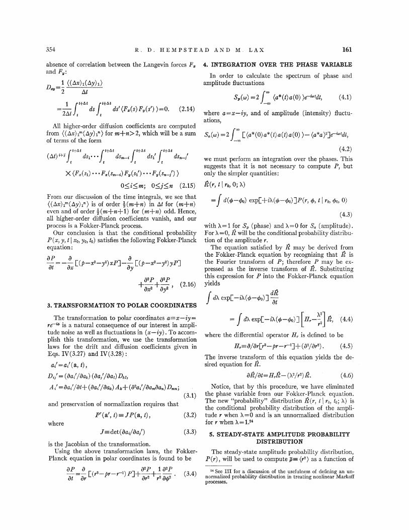
10

the dimensionless pump parameter p. This functionaldependence, shown in Fig. 1, allows the experilnenterto determine the value of our pump parameter p forhis oscillator by measuring the power output and usingthe appropriate scaling laws. We also use P(r) inSec. 6 for the calculation of the power spectra, and inthe eigenfunction expansion of Sec. 7.

As stated in Sec. 4, by setting X=O in Kq. (4.6),we obtain an equation for the conditional probabilityof the amplitude. Using the stationary property

lim P(r, t ) rp, tp) =P(r),(g—gp)-+m

and taking this limit on both sides of Eq. (4.6), weobtain an equation for P(r) .

TAnLE I. Mean intensity p= ( Ia I') and total intensity Quctu-

ation ((/1p) ') = (p') —(p) ' for NRWVP oscillator versus net pumpparameter p.

—109—8—7—6—5

—3—2—10123

56789

10

0.19270060.21240180.23637710.26609980.30375390.35268100.41816100.50880150.63896590.83270631.1283791 ~ 5779562.2252713 ' 0604904.0103585.0010896.0000707.0000038.0000009.000000

10.000000

((/1/)')

0.035860230.043269770.053108900.066492660.085210090.11221120.15249750.21471670.31379070.47389400.72676111.0880101.4987111.8154621.9584621.9945531.9995831.9999812.0000002.0000002.000000

=(*(O) (O))=( &=-1 " S~(/o) do/

2 2' (5 4)

if we use

f~ exp(io/t) do/

=B(t).QQ 2r

the power output /o=—(r') to our dimensionless pumpparameter p. Integrating r'P (r), numerically using(5.3), we obtain p as a function of p in the regionnear threshold. "The results are shown in Fig. 1 andTable I.

The integrated spectrum of phase and amplitudefluctuations using (4.1) can be written

gp) s- Similarly, the total amplitude noise, using (4.2), can

0 — i I I - I I I I I I

-10 -8 -8 -4 -2 0 2 4 8 8 'l0

NET PUMP RATE, p

FIG. 1. The mean amplitude squared (intensity) p—= ( Ia I2)

for the NRWVP oscillator is plotted as a function of the pumpparameter p. For a laser, p is the normalized mean number ofphotons (btb) /P, where P is defined by Eq. (A.13). The solidcurve gives our exact values. The upper dashed curve is the quasi-linear approximation, which was obtained as usual from (A (//) )~A((//)) =0 and yields pot, =-', Lp+(p'+g)'"g. Below threshold,the Gaussian nature of the radiation field suggests (pm)=2(p)lwhich yields pug=-,'Lp+(p'+16)'"j, an excellent approximationbelow threshold but a poor one above (lower dashed curve).

"In general J need not be zero, and detailed balance is notobeyed. See IV, Sec. 4 for an example in which 7&0. For furtherdiscussion of detailed balance see III, Sec. 78, and Ref. 17, Chap.8.

'6 For the relation between time-reversal, detailed balance andorthogonality, see Ref. 17, Chap. 8.

"The results for /o= (p) were also checked by expressing (//)in terms of error integrals

00 -1

(// ) p+ 2 //2 egl /4 e /2/2/tt

—pl&2

For p&0, we also have the continued fraction

lpl+

lpl+

Ipl+I pl+".

Higher moments can be computed directly or by the recursionformula

(pfL ) p ( m 1)+2(+ 1) (//eM—)

In particular, (//')=p(//)+2 and ((/1//)')= (//') —(p)' whichgovern total amplitude noise are plotted in V, Fig. 5 and QVII,Fig. 3 and quoted in Table I of this paper.

R. D. HEMI'STEAD AND M. I AX

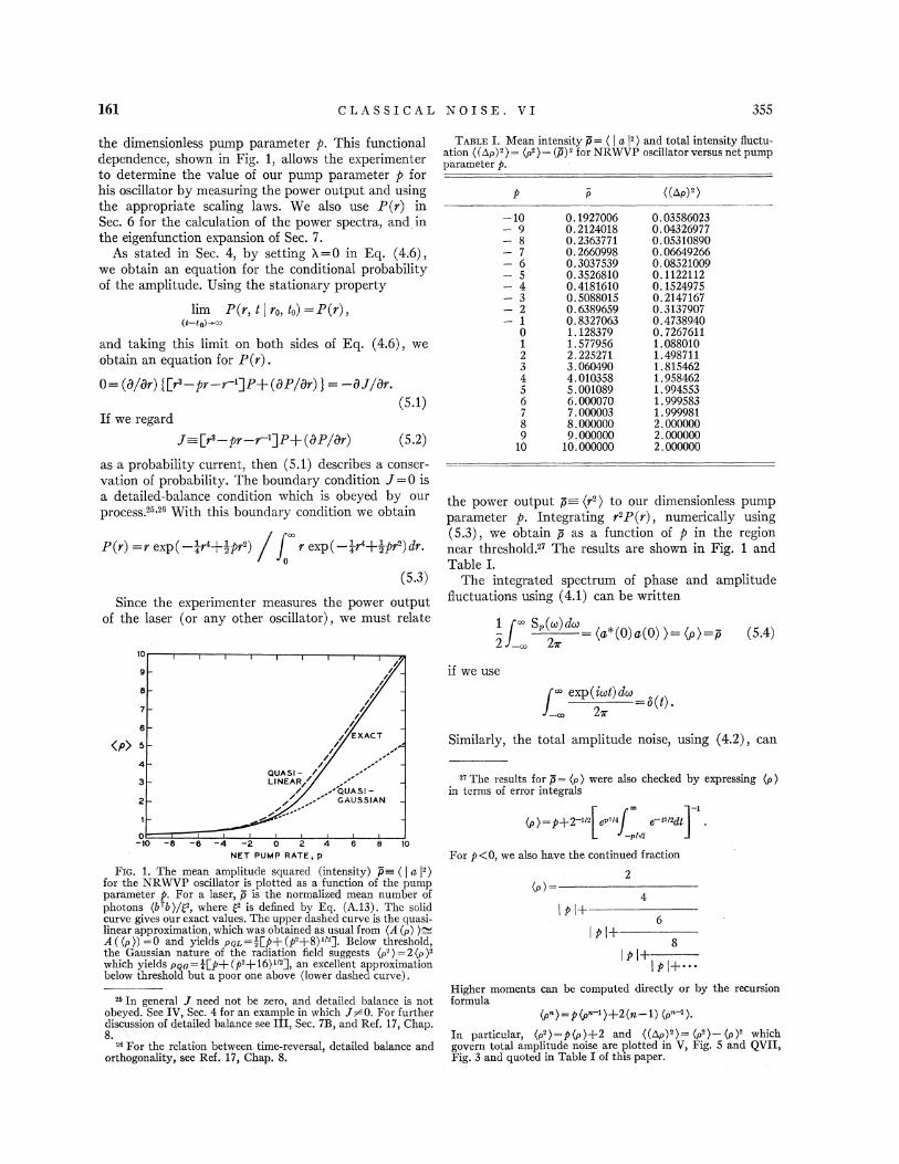
TABLE II. Spectrum Sdr (ca) for phase (and amplitude) fluctuations.

Frequency co —10Pump parameter P—1 0

00.250.51.02.05.0

10.020.050.0

100.0

0.074290.074250.074120.073610.071630.060290.038520.015760.0030680.0007916

0.82590.82050.80470.74740.58160.22810.072220.019430.0031840.0007990

1.420ie4041.3571.1990.81880.25510.074380.019560.0031870.0007992

2.6772.6182.4571.97i1.1010.27230.075220.019590.0031880.0007992

5.5355.2744.6193.0881.3330.27510.074600.019510.0031850.0007990

12.1810.858, 1794.1281.4000.26360.072580.019300.0031780.0007986

389.8367.7314.4199.080.6115.624.0331.0240.172i0.04870

~ For p=10 the correct frequency is iqth the tabulated frequency.

be written

1 S,(o)) d(p = &(~p)')=—(p') —&p)' (5 5)2 — 2Ã

The results'r for p and &(Ap)') a,re summarized inTable I.

6. CALCULATION OF THE POWER SPECTRA

We de6ne U(r) to be the homogeneous solution tothe above equation which satis6es the boundary condi-tion for G at r =0, and we define V(r) to be the homo-geneous solution which satisfies the boundary conditionfor G at r= po. The solution, G(r, rp, 'A, (d), may bewritten in terms of U(r) and V(r):

G(r, rp) =—$U(r) V(rp)/W(rp) j, r&rp

= —$U(rp) V(r)/W(rp) ), r) rp (6.4)The time integrals in Eq. (4.1) and (4.2) suggest

that we need not compute 8, which obeys a partialdiGerential equation, rather only its one-sided Fouriertransform.

where W(rp) is the Wronskian

W(r) =U(r) V'(r) V(r) U'(r)—= df r exp( —,'r'+ ', Pr'), - (6.5)

dt e-'"'A(r, t i r„0;X). (6.1)G(r, rp, X, pp) —= where A is a constant. We notice that the Wronskianis just a constant times the steady-state amplitudeprobability distribution P(r) .

The spectra S„(o)) and S,(o)) can now be computeddirectly from G(r, rp, X, o)) by the following integra-tions:

The equation obeyed by G may be obtained by takingthe one-sided Fourier transform of both sides of Eq.(4.6).

f88 x'

dt e '"'—= H„, G(r, r(), X—, o—)). (6.2)0

r' S ( )=dsef drrrrP(rr) f drrG(r, rr; 1, )0 0

d2G dG, (1—X')+ (r' pr r') —+ 3r' —p+ — —ip) G—dr dr r2

= —A(r, 0 i rp, 0; X) = t')(r r,)——dr r —p Gr ro'O, M . 6.6

0(6 5)

Equation (6.6) displays the subtraction of the t) func-tion at co =0 in the amplitude spectra, which correspondsof the Green's-function form.

The left-hand side of the above equation may be inte-grated by parts to give an inhomogeneous ordinary OO

differential equation for G: S,(o)) =4 Re drp(rp' —p) P(rp)0

7~x,z III. Spectrum S (or) for intensity Quctuations.

Frequency co

Pump parameter P1 2

01.02.05.0

10.015.020.030.050.0

100.0

0.0066800.0066650.0066220.0063360.0054890.0044890.0035770.0022630.0010410.000295

0.15710.15460.14770.11230.060790.034590.021630.010480.0039660.001014

0.27910.27290.25610.17920.087180.047360.029020.013840.0051930.001323

0.49660.48170.44210.28170.12490.065780.039850.018860.0070500.001794

0.82600.79450.71330.42010.17630.091880.055570.026310.0098460.002508

l.1581.1100.98780.56860.23950.12630.076970.036730.013830.003533

1.1011.0751.0020.69560.35430.20250.1284Oe063540.024500.006337

0.71220.70590.68780.58470.38600.25020.16920.088880.035640.009409

0.51740.51510.50840.46630.36060.26270.19110.10820.045730.01241

Oe40530.40420.40100.37980.31980.25340.19670.12040.054080.01519

CLASSICAL NOI S E, VZ 357

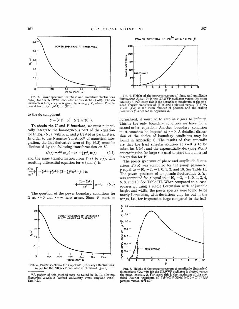
POWER SPECTRA OF t'e AT QP 0 VS P

2.0

3 1.5C1.

CA

1,0

0.5

SHOLD 250

200D

150

100

O50

I

2.0I I

4.0 6.0FREQUENCY cu

I

8.0 10.000 1 2 3 4 5 6 7 8 9 10

P

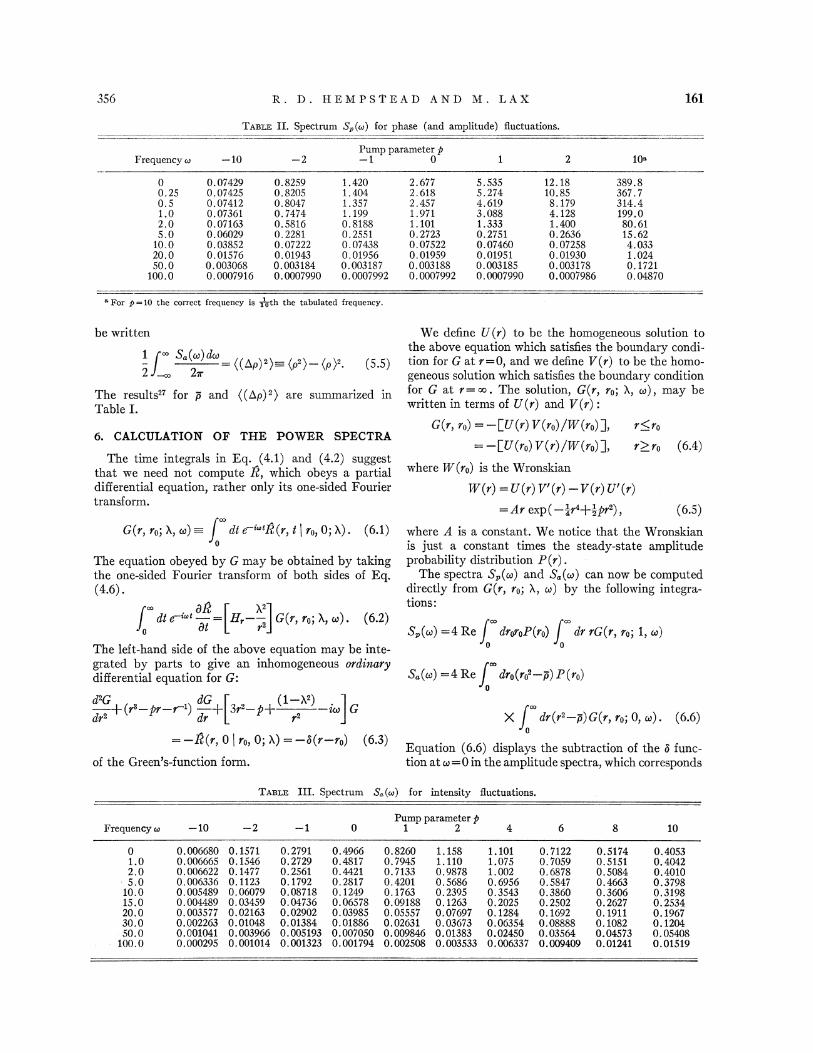
FIG. 2. Power spectrum for phase and amplitude fluctuationsS„(au) for the NRWVP oscillator at threshold (p=0). The di-mensionless frequency eo is given by co=or, ~ T, where T is ob-tained from Eqs. (A14) or (813).

to the dc component

p2 (y2)2 of (y2(f) y2(0) )To obtain the U and V' functions, we must numeri-

cally integrate the homogeneous part of the equationfor 6, Eq. (6.3), with X, ce, and p treated as parameters.In order to use Numerov's metnod" of numerical inte-gration, the first derivative term of Eq. (6.3) must beeliminated by the following transformation on U.

U(y) =y"' exp( ——',y'+-', py')N(y) (6.7)

and the same transformation from V(y) to e(y). Theresulting differential equation for se (and v) is

+ —reys+Psry4+ (2—r Ps) ys —P+s(g

(1—4Xs)+, I=0. (6.8)

The question of the power boundary conditions forQ at r=0 and r=~ now arises. Since P must be

PxG. 4. Height of the power spectrum of phase and amplitudefluctuations S„(or=0) in the NRWVP oscillator versus the meanintensity P. For lasers this is the normalized maximum of the one-sided Fourier transform of (bt(e)b(0) ) plotted versus (btb)/fe,where (btb) is the mean number of photons and the scalingparameter P is dehned in Appendix A.

normalized, it must go to zero as r goes to ininity.This is the only boundary condition we have for asecond-order equation. Another boundary conditionmust somehow be imposed at r=0. A detailed discus-sion of the choice of boundary conditions may befound in Appendix C. The results of that appendixare that the least singular solution at r=0 is to betaken for U(y), and the exponentially decaying %KBapproximation for large r is used to start the numericalintegration for t/'.

The power spectrum of phase and amplitude Quctu-ations S„(~) was computed for the pump parameter

p equal to —10, —2, —1, 0, 1, 2, and 10. See Table II.The power spectrum of amplitude fluctuations S,(co)

was computed for p equal to —10, —2, —1, 0, 1, 2, 4,6, 8, and 10. See Table III. %hen compared to a least-squares 6t using a single Lorentzian with adjustableheight and width, the power spectra were found to benearly Lorentzian, with deviations only far out in thewings, i.e., for frequencies large compared to the half-

0.5

0.4TENSITY

SHOLO

0.53C$

CA 0.2

0.1

5.0l

10.0 15.0 20.0FREQUENCY M

l 1

25.0 50.0

Fro. 3. Power spectrum for amplitude (intensity) fluctuationsSo(&o) for the NRWVP oscillator at threshold (p=0).

~SA review of this method Inay be found in D. R. Hartree,Nsssaeyeeol ANofyses (Oxford University Press, England 1958),Sec. f.23.

1.4s3

1.2

IO 1,0-I

o.e0~~0.8—tK

+~ 0.4—O.Ol

a: 0.2-O

2 3 40 I 5 B 7

PFro. $. Height of the power spectrum of amplitude (intensity)

fluctuations S (co=0) for the NRWVP oscillator is plotted versusthe mean intensity p. For lasers this is the maximum of the one-sided Fourier transform of P (bt (0)bt (t) b (1)b (0) )—(btb )'7/$4plotted versus (btb )/1st

R. D. HEMP STEAD AND M. LAX

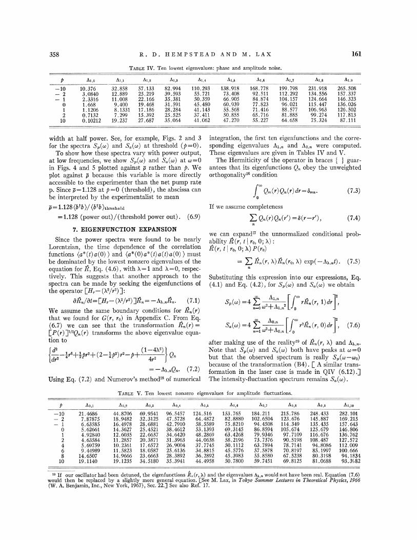
TABL,E IV. Ten lowest eigenvalues: phase and amplitude noise.

—10—2—10

210

A],o

10.3763.08402.33161.6681.12060.71320.10212

32.85812.88911.0089.4008.13317.299

19,237

312

57.13325.21922. 16619.46817.18615.39227.687

A1 3

82.99439.59335.38131.59128.28425. 52535.064

110.29355.72150.35945.48041.14337.41141.062

~1,5

138.91873.40866.90560 ' 93955.56850.85547.270

A16

168.77892.51184.87477.82371.41665.71655.227

h.1 7

199.798112.292104.15796.02188.57781.88564.658

h.1 8

231.918134.556124.664115.447106.96399.27475.324

A1 g

265.508157.337146.323136.026126.502117.81387.111

width at half power. See, for example, Figs. 2 and 3for the spectra S„(&p) and S,(cp) at threshold (p=O).

To show how these spectra vary with power output,at low frequencies, we show S„(cp) and S (&p) at cp=0in Figs. 4 and 5 plotted against p rather than p. Weplot against p because this variable is more directlyaccessible to the experimenter than the net pump ratep. Since p=1.128 at p=O (threshold), the abscissa canbe interpreted by the experimentalist to mean

p =1.128 (btb )/ (b"b )sgre, g, )p

=1.128 (power out)/(threshold power out) . (6.9)

7. EIGENFUNCTION EXPANSION

Since the power spectra were found to be nearlyLorentzian, the time dependence of the correlationfunctions (a*(t)a(0) ) and (a*(0)a*(t)a(t) a(0) ) mustbe dominated by the lowest nonzero eigenvalues of theequation for R, Eq. (4.6), with it=1 and it=0, respec-tively. This suggests that another approach to thespectra can be made by seeking the eigenfunctions ofthe operator [H, (lt'/r') j:—

BR„/Bt= [H„(lt'/r') jR„=—Ag, „R„. (—7.1)

We assume the same boundary conditions for 8„(r)that we found for G(r, rp) in Appendix C. From Eq.(6.7) we can see that the transformation 8„(r)=[P(r) Ji'Q„(r) transforms the above eigenvalue equa-tion to

I 6 1 (1—4lt')1rp+ 1prp+ (2 r pp) rp p+ Q4 2 4r'

= —Ag, „Q„. (7.2)

Using Eq. (7.2) and Numerov's method" of numerical

Q (r) Q„(r)dr = b „. (7.3)

If we assume completeness

Z Q-(r) Q-(") =b(» —"), (7 4)

we can expand'~ the unnormalized conditional prob-ability R(r, t

t rp, 0; lt):8(r, t

( rp, 0; lt) P(rp)

= g R (r, l~)R„(rp, lt) exp( —Ay, „t). (7.5)

Substituting this expression into our expressions, Eq.(4.1) and Eq. (4.2), for S„(cp) and S,(cp) we obtain

S„(cp) =4 Qn pep +At,=n

OO 2

rB„(r, 1)dr

S,(cp) =4 Qn,=l cp +Ap, m

00 2

r'8 (r, 0)dr, (7.6)

after making use of the reality" of R„(r, X) and Az, .Note that S„(cp) and S (pp) both have peaks at cp=obut that the observed spectrum is really S„(cp—cpp)

because of the transformation (B4) . [A similar trans-formation in the laser case is made in QIV (6.12).)The intensity-fluctuation spectrum remains S,(cp) .

integration, the erst ten eigenfunctions and the corre-sponding eigenvalues A~,„and Ao,„were computed.These eigenvalues are given in Tables IV and V.

The Hermiticity of the operator in braces I I guar-antees that its eigenfunctions Q„obey the unweightedorthogonality" condition

TABLE V. Ten lowest nonzero eigenvalues for amplitude fluctuations.

—10—21012468

10

&01

21.46867.878756.635855.626614.928404.635845.697599.44989

14.650719.1140

AO2

44.870618.948216.497814.362712.603511.285710.236111.582314.966619.1235

~0,8

69.954132.312528.688125.452122.663720.387117.657218.058723.666334.5180

Ao4

96.545747. 572842. 791038.461234.642031.396326.900425. 613628.389235.3941

h.o 5

124.51664.487258.558953.139348.286944 ' 063837.774534.881536.289244.4958

Ao, 6

153.76582.888075 ' 821069.314563.426858.219650. 111245.577645.398350.7800

AO7

184.211102.650494.450886.859479.934673.737663.789457.587855.858059.7451

~o,s

215.786123.676114.349105.67497.710990.519878.714170.819767.523869.8125

hog

248. 433145.887135.435125.679116.676108.48794.808685. 199780.319881.0688

~0,10

282. 101169.215157.643146.806136.762127.572112.009100.66694. 183493.3982

A"If our oscillator had been detuned, the eigenfunctions R„(r, ) ) and the eigenvalues A~, would not have been real. Equation (7.6)would then be replaced by a slightly more general equation. /See M. Lax, in Tokyo Sesaraer Lectures isc Theoretical Physics, lp66{W.A. Benjamin, Inc. , New York, 1967), Sec. 22.j See also Rei. 17.

CLASSICAL NOISE.

IoX

o

IoXlE)

o

XlE)oo

Xo

o

I

X

o

'M

I

Xo

X

o

X

o

IoXo

o

XChCV)

o

X

o

XQO

o

X

o

X

o

X8o

X

o

X

o

IoXoo

X

o

oX

o

X

o

o'

X00

o

IoX

o

X

o

CO

CI Xooo

IoX

o

IoX

o

X

o

CO'MIoX00

o

X00

o

X

ooo

Xoo

Xoo

O~ W

cd

3V

cd

C4

cd

a8O~

8C4

cd

82

.9O

O8

O

O~ ~

O

cd

O~ pf

A

CO

4

l/)

LC)

o

'M

IoXCh

o

Xooo

Xo00o

IoX

o

X00QO

o

o o

IoX

o

CO

I

X00

o

T

X

o

I

X

o

X

2o

X

00o

IoX

o

I

X

o

IoXo

o

IoX

o

I

X X o

oX

o

X

o

oIXP0

X

o

IoXoo

X

o

o

IoX

o

IoX

QO

o

oIXoo

Xo

o

oX

o

IoX

o

oIXo

o

IoX(V)

o

o7X

o

X00lPj

o

o

X

o

IoX

o

(V)

o

X

o

82V

C4

0&

~ W

C4

O

O8

A

O

O~ H

OV

O

Vcd

aCl

~D

aQ

C)

oo

X

o

X

o

l/)

o

oo

LX

o

X

o

oXoo

oo

IoX

o

lE)

o

X

o

Xolt)o

IoX

o

X

o

oX

o

00

o

Xo

o

X

o

IoX0000

o

IoXoo

uD

o

o

aI

X

o

X00oo

oIX

o

I

X00

o

7

X

o

Xoo

oTXChoo

o

o|"XCV)

oo

Xo

o

IoX00oo

X

X

o

00o

X

o

X

00o

IoX

oo

|"oX

o

4'

o

IoX

o

X00

olE)

o

IoXoo

IoX

o

IoX

o

X

o

Xo

o

o

IoXo00

o

oo

7

X00

o

X00lE)

o

oIX00

o

X

o

X

o

X00

o

X00

o

I

X X

o o

Xo

o

IoXCh

o

o'

Xoo

Xo

X

o o o oVO

o oo8o

o

o00

o o

o

o

oCh

o o o

o

o

oVO

00o

QO

00o o

oo o o

o o

R. D. HEMPSTEAD AND M. I, AX

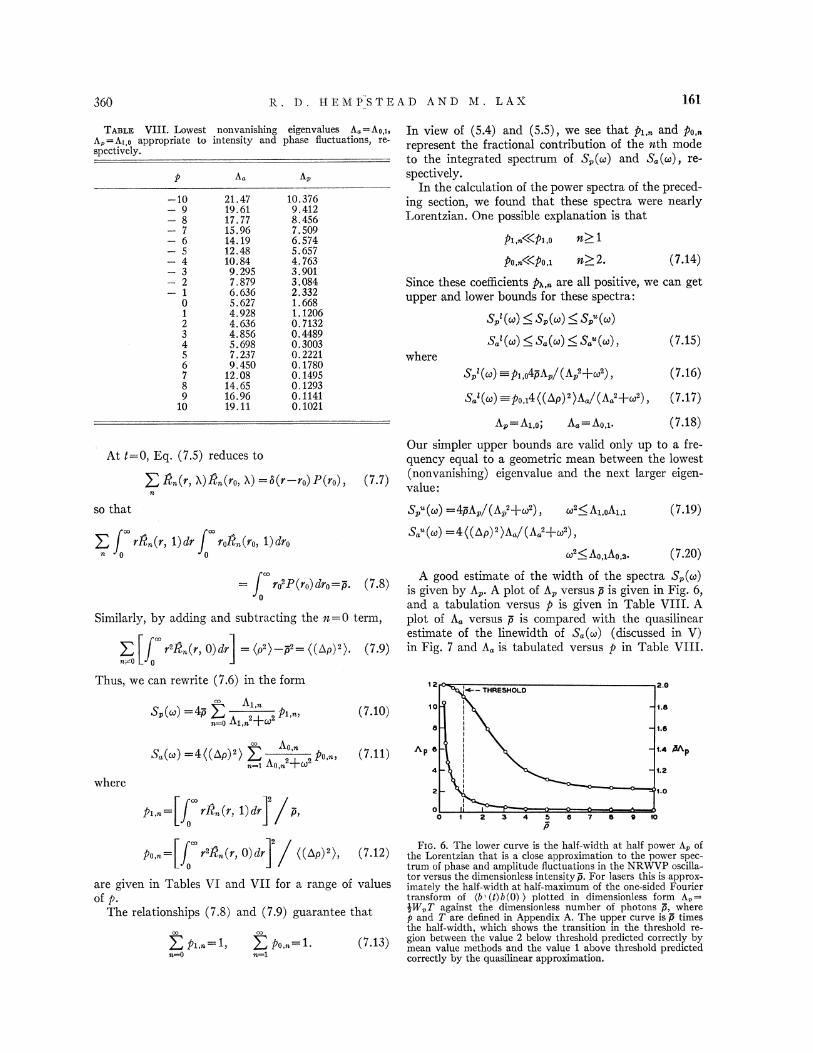
—10—9—8—7—6—54—3—2—10

23456789

10

21.4719.6117.7715.9614.1912.4810.849.2957.8796.6365.6274.9284.6364.8565.6987.2379.450

12.0814.6516.9619.11

10.3769.4128.4567.5096.5745.6574.7633.9013.0842.3321.6681.12060.71320.44890.30030.22210.17800.14950, 12930.11410.1021

TABLE VIII. Lowest nonvanishing eigenvalues A, =Ao, &,

A„=A10 appropriate to intensity and phase fluctuations, re-spectively.

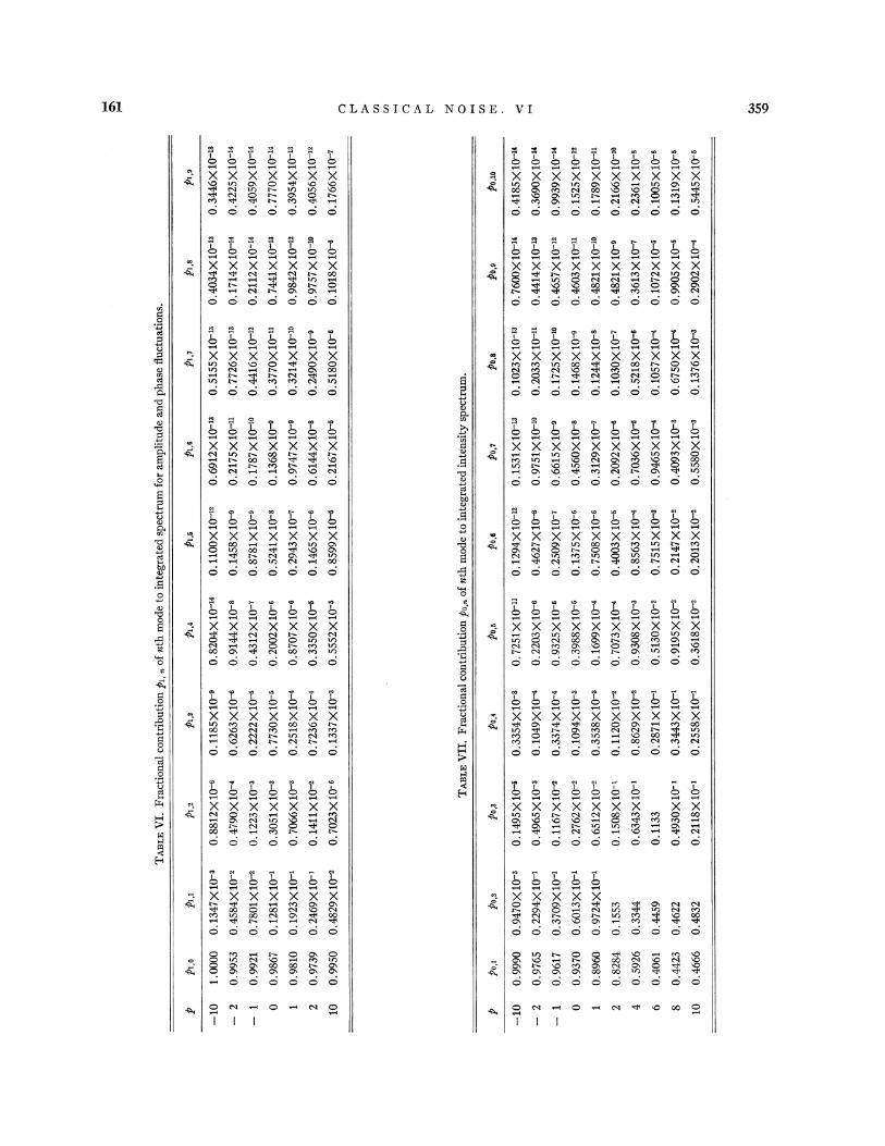
In view of (5.4) and (5.5), we see that pr, „and po,„represent the fractional contribution of the nth modeto the integrated spectrum of S„(co) and S, (oo), re-

spectively.In the calculation of the power spectra of the preced-

ing section, we found that these spectra were nearlyI.orentzian. One possible explanation is that

pi, «pi, o

po,a«po, x (7.14)

where

S,'(co) & S„(a))& S~"(co)

S.'(I) (S,((o) (S. ((v),

S„'(oo) =—p),o4pA„/(A„'+oo'),

(7.15)

(7.16)

S '( )—=po, 4((hp)')A, /(A. '+ '), (7.17)

Since these coefIicients px,„are all positive, we can getupper and lower bounds for these spectra:

h.y =Al, 0' A =A.0,l. (7.18)

At t=0, Eq. (7.5) reduces to

Q 8„(r, X)8„(ro, X) =8(r—ro)1 (ro), (7.7)

Our simpler upper bounds are valid only up to a fre-quency equal to a geometric mean between the lowest(nonvanishing) eigenvalue and the next larger eigen-value:

so that S„"(oo) =4ph.„/(A„'+oP), Or'& h.l,PA.l, l (7.19)

r8„(r, 1)dr roR„(ro, 1)dr,n 0

rooP(ro) dro= p. (7.8)

Similarly, by adding and subtracting the e=o term,

r'8„(r 0) dr = (p') —p'= ((dp)'). (7.9)n&0 0

Thus, we can rewrite (7.6) in the form

(o'& Ao, ~ho, o. (7.20)

A good estimate of the width of the spectra S„(co)is given by A„. A plot of A„versus p is given in Fig. 6,and a tabulation versus p is given in Table VIII. Aplot of A, versus p is compared with the quasilinearestimate of the linewidth of S,(~) (discussed in V)in Fig. 7 and A, is tabulated versus p in Table VIII.

Al,„So(~) =4p Q, '",pi...

n-o Al, m

(7.10) 10

where

S.(«) =4((~p)') Q,'",po. ,1 Aon +~ (7.11) Ap b —1.4 gfA&

—1.2

pl, m

0

r8„(r, 1)dr 0 1 2 3 4 5 e 7 S 9 10P

po, n

0

r'8 (r, 0)dr ((Ap)') (7 12)

P p, ,„=1,n=O

(7.13)

are given in Tables VI and VII for a range of valuesof p.

The relationships (7.8) and (7.9) guarantee that

FlG. 6. The lower curve is the half-width at half power A.„ofthe Lorentzian that is a close approximation to the power spec-trum of phase and amplitude fluctuations in the NRWVP oscilla-tor versus the dimensionless intensity p. For lasers this is approx-imately the half-width at half-maximum of the one-sided Fouriertransform of (b'(t)b(0) ) plotted in dimensionless form A~=)lV„T against the dimensionless number of photons p, wherep and T are de6ned in Appendix A. The upper curve is p timesthe half-width, which shows the transition in the threshold re-gion between the value 2 below threshold predicted correctly bymean value methods and the value 1 above threshold predictedcorrectly by the quasilinear approximation.

24

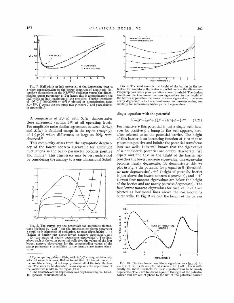
CLA S SgCAL NOISE.

50 I I I I

E IGENVALUESBARRIER HEIGHTp20 6 40

30

20

4I

II

7 s 9 102/7

lf er A of the Lorentzian thatht d ('-

en in NRWVP oscillator versus ttion to the power p

y) in thethe

h o id d Fo t fo1ttd '

d io1rate~ where 7 and p are de6ned=-'O' T versus the net pump rate p, w erehg=g g

in Appendix A.

arison of 5„"(~) with S„(~) demonstratesdo g (within 3 0 a a

noise similar agreement e w.() o d p0f 2&p&6 where differences as large as

rises from the asymptotic degener-alue for amplitudeest nonzero eigenva ue

~ ~

b b d dhis de eneracy may e es

by considering the analogy to a one- ime

50—

40-

30-

& 20-

Z 10-I-O0

-100

I I I I

2 3 5PUMP PARAMETER p

10

dinger equation with t phe otential

7.21)V = sr rs 'Pr4+ (—-'P—'—2) r'+P —4r

this otential is just a sing e mmell how-h dl, hever o po tve p

of this b

htth 1

'iveandin nite epo

s. It is well known t a ed bl d t W

h'ht fth b-ll otential are ou y

that as the eig oexpect and find thnvalue this eigenvalue

'ht f potential barrier

8 the otential or equa~ ~

no near degeneracie S 6 elg 01 ) and +10west nonzero eigenva ue,is just above the lowes

below the heightzero ei envalues are e owd t) Thnearl air wise eg

, l.tth, h„h.f h, b„„„outer wells. In Fig. 9 we plot t e eig

the height of the barrier in t pot 1 for amplitude Quctuations p

b threshold. The dashedess pump parameter p o pei envalues. As the heigcurves are t e o

owest nonzero eigenva ue, i

four lowest nonzero g . it becomesthe barrier approaches t ed 1 t nonzero eigenvalue, annearly degenerate w'

h' her airs of eigenvalues.similarly for successively ig e p

-10-

-200.1 0.5 1.0 1.5 2.0

AMPLITUDE, r2.5 3.0

p a+10

4.0

e otentia s o'

1 f r amplitude Quctua-pIG.

cillation, no near degeneractes),P q ~ o - ~ -:'Dl -t ~ "- ~ .1 ), ~ d{h ht f barrier gust above owesde enerate eigenv+o( op

es for the corresponding valueouter otential we s give

es of theth t ad -t t ( 0)pump parameter p

' tin addition to evalue.

C4

ClII

CLILOtL

a

O

1.0—.8- &

/.6 -I

I gn=24 $PEAK.2 P

0-

r 0 dr, wit pr, 'h ~(h )') using variationally

e'

d th t the lowest mode, inRisken foun ase ec e1 t 11 fth tot 1A tdid not supply a mos a a

bdb1 1' h

h db WL bt e owe

f this degeneracy was emp"The existence o isJr. (private communication),

I II

4-1.0

1 2AMPLITUDE, r

litude eigenfunctions r for'IG. 10. The two lowest amphtu e 'g.2 are plotted versus r or

for these eigenfunctions to eto th }1tof thd ate. The wave functions agreegenera

f hase to the e o.bg,rrier and are opt o p

362 R, D. HEM P STEAD AND M, LAX

i.5

t lP=+10

.9/.8 I

0.6 I.5 l4

/ \

.2 ~sr

0 2 4AMPL ITUDE, V

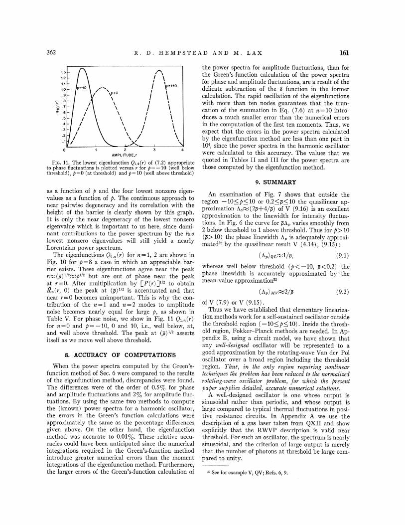
FIG. 11. The lowest eigenfunction Q1,0(r') of (7.2) appropriateto phase fIuctuations is plotted versus r for p= —10 (well belowthreshold), p=0 (at threshold) and p=10 (well above threshold)

1.2

1.0

8. ACCURACY OF COMPUTATIONS

When the power spectra computed by the Green's-function method of Sec. 6 were compared to the resultsof the eigenfunction method, discrepancies were found.The differences were of the order of 0.5%%uo for phaseand amplitude fluctuations and 2%%uo for amplitude fluc-tuations. Sy using the same two methods to computethe (known) power spectra for a harmonic oscillator,the errors in the Green's function calculations wereapproximately the same as the percentage differencesgiven above. On the other hand, the eigenfunctionmethod was accurate to 0.01%. These relative accu-racies could have been anticipated since the numericalintegrations required in the Green's-function methodintroduce greater numerical errors than the momentintegrations of the eigenfunction method. Furthermore,the larger errors of the Green's-function calculation of

as a function of p and the four lowest nonzero eigen-values as a function of p. The continuous approach tonear pairwise degeneracy and its correlation with theheight of the barrier is clearly shown by this graph.It is only the near degeneracy of the lowest nonzeroeigenvalue which is important to us here, since domi-nant contributions to the power spectrum by the tmo

lowest nonzero eigenvalues will still yield a nearlyLorentzian power spectrum.

The eigenfunctions Qs „(r) for n=1, 2 are shown inFig. 10 for p=g a, case in which an appreciable bar-rier exists. These eigenfunctions agree near the peakr~(p)'t'~p't' but are out of phase near the peakat r=0 After .multiplication by PP(r)]'t' to obtainA„(r, 0) the peak at (p)"' is accentuated and thatnear r=0 becomes unimportant. This is why the con-tribution of the m=1 and v=2 modes to amplitudenoise becomes nearly equal for large p, as shown inTable V. For pha, se noise, we show in Fig. 11 Qt,„(r)for n=0 and p= —10, 0 and 10, i.e., well below, at,and well above threshold. The peak at (p)'ts assertsitself as we move well above threshold.

the power spectra for amplitude fluctuations, than forthe Green's-function calculation of the power spectrafor phase and amplitude fluctuations, are a result of thedelicate subtraction of the 8 function in the formercalculation. The rapid oscillation of the eigenfunctionswith more than ten nodes guarantees that the trun-cation of the summation in Eq. (7.6) at n=10 intro-duces a much smaller error than the numerical errorsin the computation of the first ten moments. Thus, weexpect that the errors in the power spectra calculatedby the eigenfunction method are less than one part in104, since the power spectra in the harmonic oscillatorwere calculated to this accuracy. The values that wequoted in Tables II and III for the power spectra arethose computed by the eigenfunction method.

9. SUMMARY

An examination of Fig. 7 shows that outside theregion —10&p&10 or 0.2&p&10 the quasilinear ap-proximation A, (2p+4/p) of V (9.16) is an excellentapproximation to the linewidth for intensity fluctua-tions. In Fig. 6 the curve for pA„varies smoothly from2 below threshoM to 1 above threshold. Thus for p) 10(p) 10) the phase linewidth A„ is adequately approxi-mated" by the quasilinear result V (4.14), (9.15):

(tt.)etc=1/p, (9.1)

whereas well below threshold (p( —10, p(0.2) thephase linewidth is accurately approximated by themean-value approximation"

(Ap) srv~2/p (9 2)

''-See for example V, QV; Refs. 6, 9.

of V (7.9) or V (9.15).Thus we have established that elementary lineariza-

tion methods work for a self-sustained oscillator outsidethe threshold region ( —10&p& 10) . Inside the thresh-old region, Fokker —Planck methods are needed. In Ap-pendix 8, using a circuit model, we have shown thatany mell-designed oscillator will be represented to agood approximation by the rotating-wave Van der Poloscillator over a broad region including the thresholdregion. Thus, ie the oddly region requirirIg eoelieeurtechniques the proMem has been reduced to the nornsaHsedrotating wave oscillator -problem, for which the presentpaper supplies detaited, accurate nunMricat solutions.

A well-designed oscillator is one whose output issinusoidal rather than periodic, and whose output islarge compared to typical thermal fluctuations in posi-tive resistance circuits. In Appendix A we use thedescription of a gas laser taken from QXII and showexplicitly that the RWVP description is valid nearthreshold. For such an oscillator, the spectrum is nearlysinusoidal, and the criterion of large output is merelythat the number of photons at threshold be large com-pared to unity.

CLASSICAL NOISE. VI 363

J,= (r, -w„)/~,

J,= (r,-w„)/~,

rl F2 w12w21+2r (F1+F2 w12 w21) Ii

(A2)

The radiative rate constant m is such that the rate ofdownward transitions are 2rX2(I+1) whereas the rateof upward transitions are xX1I where S2 and X1 arethe upper and lower state populations and (I)=( ( P i2) = (number of photons). The nonradiative tran-sition rate from 1~2 is m12. The total decay rate outof state 1 (or 2) excluding the radiative rate to 2 (or 1)is F, (or F,).

Typical parameters" for a gas laser are F1, I'2 10'sec ', 2r (1/10) sec '. From the quasilinear treatmentof QVII L(6.S)—(6.7) j and Eq. (A18) below we seethat the number of photons at threshold is of order(I"2/2r)"'. The nonlinearity in Ji and J2 is of the form

(F,+2rI) ', Where

rs (rlr2 w12w21) /(F1+F2 w12 w21) i (A3)

so that near threshold mI((F, and we may expand J&

and J2 keeping terms linear in I. In this region, thenoise sources 2r J2G2 (2r/F, )G, and 2r J161 are entirelynegligible. Our Langevin process then reduces to thefolol

dP/dt = ', (1 i )Py I II -Ro —i P i'}+Gp,— (A4)

"See. D. E. McCumber, Phys. Rev. 141, 306 (1966) and Table1 of QVII.

APPENDIX A' THE LASER MODEL

In QXII, Lax and Louisell study a model for a maserin which the Fokker-Planck equation for the associ-ated classical function P(p, p*, Ni, N2, t) which corre-sponds dynamically to the density matrix of the electro-magnetic field and atomic population variables. TheLangevin equations for this Fokker-Planck process areobtained. For a gas laser, the atomic response ratesare fast compared to the photon rates so that thepopulation variables E1 and X2 follow the instantane-ous value of the radiation Geld. Thus, an adiabaticapproximation for the population variables yields aI'okker —Planck equation for the associated classicalfunction P(P, P*, t) which corresponds dynamicallyto the density matrix of the electromagnetic Geld

p(b, bt, t).The Langevin equations corresponding to the

P(P, P*, t) Fokker-Planck process are found to havethe form

dP/dt=2(1 2') pI ——y+2rE(R2+G2) J2—(Ri+Gi) J1J}

+Gp, (A1)

where n is a measure of the detuning (which we shallset equal to zero in this paper), R2=Xw2o and Ri =ownare the pump rates into the upper (2) and lower (1)states, respectively, and

where

(2r& R2(F1—w12) —Ri(F2 —w21)II=I —i

~1~2 ~1221(AS)

(2r R2(F1—w12) —Ri(I'2 —w21)R,=i—

~1~2 ~12~21

and

X i, (A6)2r ( F1+F2—w12 —w21) )

I 1I 2 12~21 )

(Gp(t)*Gp( ) )=2Dp p~(t —)

2Dp. p yn+——2rN2

R2 (1+w21R1/I'1)=Vn+~ r, 1—(w„w„/r, r,)

'

where E2 is the adiabatic value of N2 and

(A7)

(A8)

da/dr = (1 ia) a—(p 1a p—) +h(r),

(h*(r) h(r') )=4b(r —r'),by choosing

8= (Dp*p/VR2) "',

T=2 (yRpDp ep) '12,

p = rj. 'll. —

(A11)

(A12)

(A13)

(A14)

(A15)

All calculations of this paper set a=0, i.e., neglectdetuning. In Table I we find that p= ( i a i2)=1.128when p=0, so that at threshold ( i P i2) =1.128P.

To see the order of magnitude of the above expres-sions, let m12=m21=81=0, so that

whereII= (R2/Rg) —1,

R, =yr2/~

(A16)

(A17)

is the threshold pump rate. Then

P = (r,/22r) 'I'L1+ (nR,/R, ) j'I'

p =2pp+ (nR,/R, ) j-1L1—(R,/R, )).(A18)

(A19)

Thus we see that the spectrum associated with(bt (t) b (0) ) and the intensity spectrum associatedwith (bt (0) bt (t) b(t) b(0) )—(btb)' are, aside from scal-

ing factors (P and $4, respectively) just the classicalspectra associated with (a*(t)a(0) ) and (r (t) p(0) )—(p)', respectively. Moreover, one can avoid the use of(A1S (A19) if one plots not against pump rate butagainst p=1.128(btb)/(btb), h„ i.e., against the numberof photons relative to the number at threshold.

n =(exp (5(op/h T) —1g—' (A9)

describes the blackbody noise of the electromagneticfield at the frequency oro of oscillation.

Under the scale and time transformations

P=)a, t= Tr, (A10)

our equation can be made to take the canonical form

364 R. D. HEMP STEAD AND M. LAX 161

To assess the accuracy of our expansion of J& andJ2 to linear terms, we compare the ratio of the firstneglected terms to the erst retained term:

(orI/P, ) s/(7rI/I', ) =orI/P, p/(2P) .Since p is of order unity in the threshold region, we seethat the Grst neglected term has relative importance1/P 1/(number of photons at threshold). In a well-designed laser, the number of photons at threshold islarge (10' or 104) and the neglected terms are un-important.

APPENDIX B:THE CIRCUIT MODEL

%e review here a general model of a self-sustainedoscillator, and examine the reduction of its equationsof motion to the Langevin equation for the normalizedrotating-wave Van der Pol (NRWVP) oscillator s4

While this approach is motivated by the study of lasernoise by Lax and Louisell, it is to be viewed as a studyof the extent to which the noise analysis of this papermay be applied to other self-sustained oscillators. Spe-cifically, if the equation of motion of a self-sustainedoscillator is of the type studied below, with suitablescaling parameters this paper gives the power spectraof the fIuctuations in that oscillator for operation nearthe threshold of oscillation. We will find that the basisfor this generality is the relative narrowness of thethreshold region, which is analogous to a phase transi-tion.

Let us consider an oscillator that possesses no react-ance other than that associated with a tuned circuit,but which contains a nonlinear resistance" which is afunction of a control parameter D. Using the standardnotation for the circuit parameters, the equation ofmotion is

L(dI/dt) +C 'Q+R(D) I=e(t), (B1)where e(t) is a fluctuating voltage source assumed tohave the following properties:

(1) e(t) is a Gaussian random variable of meanzero, i.e., (e(t) )=0.

(2) The power spectru'm of e(t),

Re4 (e*(t)e(0) )e-*'"'dt,

is approximately independent of oo for [ to —too~

&1/A,where h. is a characteristic decay time of the circuit.

We must now examine R(D) . The control parametercould depend upon the history of the circuit. Whilethis case is common (e.g. , solid-state lasers), we shalltreat here only those oscillators for which an adiabatic

~ See V and Ref. 17.'~ The reactance and the frequency dependence of the resistance

(omitted here) were shown in V (3.22) to have the sole efI'ect ofintroducing a detuning parameter /the n in (A.11)jwhich couplesamplitude and phase Quctuations. Since the numerical work inthis paper omits detuning, we can start directly with the Eq.(8,1) rather than the more general V (3,1i),

approximation may be made which will allow us toexpress D in terms of the instuetuneols excitation ofthe circuit. "Thus,

RLD(~) 7—=RLQ(t) I(t) 7 (B2)

For a high-Q circuit the harmonic content of theoutput may be neglected. In order to identify thisharmonic content we introduce complex amplitudes aand u*. By analogy with the definition of the creationand annihilation operators of the electromagnetic field,we de6ne a and a~ to be

u =I—i~oQ; u*=I+i&ooQ, (83)where coo is the resonant frequency of the circuit. Inthe absence of fluctuations, a would contain only thenegative frequency —coo, and u* would contain onlythe positive frequency +too. The introduction of fluc-tuations smears out the power spectra of u and a*about —too and +ooo, respectively. We seek a "pure-spectrum" solution of the form

u=A exp( itoot); —u*=A* exp(+icosa), (B4)

where A and A* are to be slowly-varying functions oftime. We can now expand R(Q, I)I as a polynomial inu and u* and replace u by A exp( i&sot) a—nd u* byA* exp(i&oot) to get

R(Q, I)I= ', Q LR„( )-u P) (A*)"exp( —ingot)

n=l

+R„( ) u )') *A"exp(i~~st) 7 (BS).

We see from the equation of motion for the circuit Eq.(B1) that A and A* will be slowly varying only if weneglect terms containing exp( —ingot) and exp(i@sot)for m&2. Thus, the harmonic content of the output isneglected by taking"

R(Q, I)I~-,'Rt() u I') (u+u*) =R(

)u (')I (B6)

where Rt(~

u ~') is required to be real by the constraintthat R(Q, I)I contains no reactive part.

The equation of motion may be further simplifiedby restricting our attention to the region of operationnear threshold. If we make a Taylor-series expansionof the nonlinear resistance about the operating pointpo Lsee, e.g., V (8.19)7 where p—=

I u )' and neglect allsecond-order and higher-order terms, we obtain

R(p) =R(po)+L~R(po)/r)po7(p po) =Rop —& —(B&)

where

Ro= E~R(Po) /r)pr 7i ff =PopR(po) /r)&o7 R(Po)~—(Bs)

'6 Our results will not depend on the adiabatic approximation,since, in the vicinity of threshold, amplitude and phase Auctua-tions become slow, so that D will in general be able to followthem instantaneously.

"The choice 2( I a P) I is equivalent to assuming that the non-ljnearity depends primarily on the energy stored jn the ctrcgif. ,

365

where"

F,(t) =L'e(t) c—ostppt; F„(1)—= L'e(t) sin—tppt.

(811)

As for the laser treated in Appendix A, we canintroduce a scaling transformation to dimensionlessvariables:

a=)a', t= Tt'. (812)

The scaling can be chosen so that only one parameterp remains in the Langevin equations. This is a measureof the negative resistance in the circuit. By analogywith the laser, it is called the pump parameter. In V(Sec. 9) it is shown that the desired choice for $ andT 1s

3'= [(e') -o/2LRo]"' T'=4LV/(e') - (813)

where (e') „,is the power spectrum of the noise sourcee(t) evaluated at the resonant frequency. With thistransformation, we obtain the NRWVP oscillatorLangevin equations given in Eqs. (2.1) and (2.2),where we have dropped the primes. The pump param-eter p is defined to be II/p, and the new Langevinforces are

F,'= ( T/&) F.,and similarly for Ii„'.

(814)

"Note that the noise sources of (B.11) are those of a non-stationary process. Over a time interval dt))co0 this nonstation-ary process can be replaced, to an excellent approximation, by astationary process as discussed in V, Sec. 5. The most relevantportion of the argument is repeated here. The random forcesP, and F„of (2.1) and (2.2) are those of the "reduced" stationaryprocess whereas those of (B.til are appropriate to the originalprocess.

In order to make the rotating-wave approximation,we rewrite the equation of motion in terms of the com-plex variables a and u*:

da/dt+i(u(p+(2L) 'R(p) a=(2L) 'R(p) a*+L 'e(t).

(89)

Since u contains only frequency components centeredabout —coo, and a* appears as a driving term whichcontains frequency components centered about +ppp,we can neglect the term in a* for a suKciently high Qcircuit. Therefore, we neglect the coupling between aand u~ by neglecting the term in a* of the aboveequation and the term in u of the complex conjugateequation. This "rotating-wave approximation" mustin fact be made if we wish the solution to have noharmonic content in the absence of noise.

Substituting our linear approximation for R(p) andintroducing 2=x—iy, we obtain Langevin equationsin the variables x and y for the rotating-wave Van derPol (RWVP) oscillator:

dx/dt = —[Rp(x'+y') II]x/2L—+F,dy/dt = —[Rp(x'+y') II)y/2—L+F„, (810)

We are now in a position to treat the case wherethe noise source e(t) is not exactly white, i.e., the noisesource is not exactly delta correlated. We anticipatethat if the power spectrum of the noise source e(t) isa slowly-varying function of frequency, a Marko%andescription is approximately valid. We must, therefore,determine the diGusion coefficients. To do this, wecalculate Dx= x(t+D—t) x(—t) in the limit of At muchless than the relaxation time, 1/A, of the circuit withno negative resistance. Thus, following the iterativeprocedure of Sec. 2, the correlation of the Langevinforces enters only in the calculation of the second-orderdiffusion coefFicients. For example,

&(») i') = 8$ ds'(F, (s) F,(s') ). (815)

Substituting our definition for Ii, in terms of the noisesource e(1), Eq. (811), and introducing the powerspectrum (e') „ofe(t), we obtain

00

((»)p) =—,L2

sin'[pr(to+cop) ht](G)+Mp)

sinp[pr((o —ppp) At]

(tp tpp)

We see that if we can choose a At such that (&op)

At«A'and if the sp. ectrum (e') „ is nearly constantfor frequencies within A. of the resonant frequency,then the term in the brackets { I of Eq. (817) maybe replaced by

I I +pxht/b(pp+pip-)+8(tp —cop)], (818)

and we obtain

D„=((»)P )/2at = (e') „,/4l. '. (819)

By similar methods, discussed in V, we obtain D» ——D„and D,„=O.These are exactly the results that we wouMhave obtained if we had assumed a pure white-noisesource with a power spectrum (e') „,. This white noisevalue (819) is to be expected since we are exciting aresonant circuit so that only the frequency componentsof the noise source within the natural bandwidth A. ofthe resonant frequency will be important in excitingthe circuit. Thus, if the power spectrum of the noisesource is approximately constant over that range of

00

((») tp) =—, dtp(e') „ds ds'L2

)& exp[io& (s—s') ]-', {cos[tpp (s—s') ]+cos[tpp (s+s') ]I .

(816)

As shown in V (4.10) and V (4.11), the rapidly oscillat-ing term cos[p~p(s+s )] yields a negligible contributionif we choose At large compared to the period of theoscillation, i.e., cook)))1. With this ht, the Grst termyields

366 R. D. IIEMPS TRAD AND M. I.AX

frequencies, it must be a good approximation to re-place our noise source by white noise with a constantpower spectrum equal to the real noise source powerspectrum evaluated at the resonant frequency

From these diffusion coefBcients we see that theLangevin forces for the "reduced'"' NRWVP oscillatorhave just those correlations given in Eq. (2.3).

To see the generality of this procedure, we returnto the truncated power-series expansion of Eq. (B7).The next term in the expansion would be the second-derivative term. The ratio of the second-derivativeterm to the first-derivative term is

(p —po) L~'R( po) /rtpo' j/L~R(po) /it poj (B2O)

T=u/r~t2.

The equation for T is

(d'T/dr') +r '(d T/dr)+( p i—cv —(72/r—') ) T =O.

(C3)

(C4)

If we now scale the independent variable r by thefollowing transformation

With this approximation for q, the equation for I, Eq.(6.8), may be put into the form of Bessel's equationby the following transformations. Ke first transformto a new dependent variable

In general, our nonlinear resistance has a form

R(p) =&f(p/m), (B21)where

p= (p'+(u')'" e pxt-,'i tan —'(co/p)]

(C5)

(C6)

where p1 is a measure of the range of variation in prequired to produce an appreciable change in R(p),and f(x), f'(x) and f"(x) are all of order unity. Ourerror is then of order

(p —po)/e=(~p)/m-E((~p)')7"/pl= p /p~, (B22)

where p„ is a noise fluctuation in p. In a well-designedoscillator, the typical operating level, which is of orderp~, is made large compared to the noise p .Thus theerror due to neglecting second-derivative terms, p„/p~,will usually be small.

APPENDIX C: THE BOUNDARY CONDITION FORG(r, rp, 2, (a)

The only condition we have for a second-order equa-tion is that the probability distribution be normalized.This implies that we choose the least-singular solutionat r=0 and r=~. To do this, we must determine theasymptotic behavior of the two linearly independenthomogeneous solutions to the equation for U (and V)for small r and for large r. For convenience, we definethe coefficient of u on the right-hand side of Eq. (6.8)to be

q== —4r'+ ,' (pr4) + (2 'p-') r' —p-i(g+—(1——4&2)/4r&.

(Ci)For small r, we may approximate q by

q p i(—u+—(1—4X') /4r—' (C2)

we obtain Bessel's equation of order X. Thus, the twolinearly independent solutions for a small r are

U~ re(Pr); ——U2 ——r Yg(Pr) . (C7)

We take the least-singular solution v (r) . This is con-sistent with our detailed-balance condition in Sec. 5.

Since a similar choice of boundary conditions is nec-essary for the harmonic oscillator, our ability to calcu-late the (known) power spectra for the harmonicoscillator using the same method (and machine pro-gram) confirms the validity of our choice of boundaryconditions.

For phase and amplitude fluctuations (X=1), we findthat one solution, U1, goes to zero and the other solu-tion U2 goes to a finite, nonzero constant as r goes tozero. For amplitude fluctuations, (X=O), both U~ andU2 go to zero as r goes to zero. In both cases we takethe least-singular solution, namely U&. For phase andamplitude fluctuations this is equivalent to assumingthat the probability distribution in rectangular coordi-nates, x and y, is finite at the origin. For amplitudeRuctuations, this is equivalent to assuming that theprobability distribution in the amplitude-squared co-ordinate p is finite at the origin.

For large r, the WEB approximation is valid:

r

w+(r) =Lq(r)1 't' exp & Lq(r') Jt'dr' .

Classical Noise. VI. Noise in Self-Sustained Oscillators near Threshold

Documents