Classical Mechanics Small Oscillations

Classical Mechanics

Small Oscillations

Dipan Kumar Ghosh

UM-DAE Centre for Excellence in Basic Sciences,

Kalina Mumbai 400098

September 24, 2016

1 Introduction

When a conservative system is displaced slightly from its “stable” equilibrium position,

it undergoes oscillation. The cause of oscillation is the restoring forces which are called

into play. Restoring forces can do both positive and negative work. When the work done

is positive, the restoring forces change the potential energy into kinetic energy and when

the work done is negative, they change kinetic energy back into potential energy.

For most mechanical systems, when the system is not too far from the equilibrium, the

restoring force is proportional to the displacement (F = −kx). Such oscillators are called

linear oscillators. For linear oscillators, the oscillation frequencies are independent of the

amplitude of oscillation. Oscillator motion can be damped in the presence of resistive

forces. Resistive forces extract energy from the oscillator. For low velocities, the resistive

forces are proportional to velocity. Oscillators, whether damped or undamped, can be

driven by external agencies which continuously supply energy to the oscillator to keep it

oscillating. Such oscillators are known as “forced” or “driven” oscillators. Driven oscilla-

tors can cause amplitude of oscillation to become very large when the driving frequency

matches the natural frequency of oscillation. This is known as the phenomenon of reso-

nance.

2 Normal Modes

2.1 Equilibrium:

Consider a system with qi as the generalised coordinates. Since the system is conser-

vative, the forces acting on the system are derivable from a potential energy function

1

c©D. K. Ghosh, IIT Bombay 2

V (q1, q2, . . . , qN). Lagrange defined equilibrium as a configuration in which all generalised

forces vanish, i.e.∂V

∂qi= 0. Clearly, in such a situation, the system will not change its

configuration. However, even when Qi = 0, the system may not be stable in the sense

that if it is slightly disturbed from a position of equilibrium, it may not return to the

position of equilibrium. If it does, such a configuration is called one of stable equilibrium

- otherwise the equilibrium is unstable.

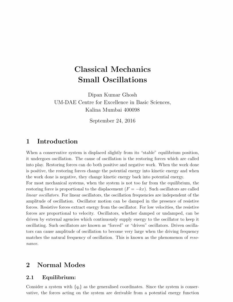
Example: Simple Pendulum

θ

V=0

x

The potential energy is given by V (θ) =

+mgl(1− cos θ), so that

F (θ) = −∂V∂θ

= −mgl sin θ = −mgx

The “generalised force” corresponding to θ in this case is actually the restring torque.

Equilibrium occurs when the restoring torque is zero. There are two such positions, θ = 0

and θ = π.

Let us look at the form of the Lagrangian near these two positions.

L =1

2ml2θ2 −mgl(1− cos θ)

Near θ = 0, cos θ ≈ 1− 1

2θ2 so that

L =1

2ml2θ2 − 1

2mglθ2

so that the potential energy is V (θ) =1

2mglθ2 and the corresponding generalised force

is −mglθ which is of restoring nature. On the other hand, near the second position of

equilibrium θ = π, cos θ = cos(π + δθ) ≈ − cos δθ = −1 +1

2δθ2. In this situation,

L =1

2ml2θ2 +

1

2mgl(δθ)2

the corresponding force is “anti-restoring”, making the equilibrium unstable.

For one dimensional holonomic systems, equilibrium can be either stable on unstable

(leaving out a trivial case of neutral equilibrium where the potential energy function is

spatially flat) for which the potential energy has an extremum

∂V

∂qi= 0 (1)


for every generalised coordinate qi. Let the position of equilibrium be qi0. If the position

is one of stable equilibrium, the potential energy has to be minimum. This is because, the

system being conservative, the total energy is constant. If we go away from the position of

minimum potential energy, it leads to an increase in the potential energy and a consequent

decrease in the kinetic energy. Thus the system returns back to the equilibrium position.

For stable equilibrium, we, therefore, have

∂2V

∂qi∂qj> 0 (2)

The converse would be true for an unstable equilibrium.

Without loss of generality, let us shift the equilibrium position to the origin (q1 = q2 =

. . . ,= qN = 0). If the system is disturbed to a configuration qi, we can write,

V (q1, q2, . . .) = V (0, 0, . . .) +∑i

(∂V

∂qi

)0

qi +1

2

∑i,j

(∂2V

∂qi∂qj

)0

qiqj + higher order terms

where the partial derivatives are evaluated at the position of equilibrium and all “higher

order terms” which involve third order or higher corrections are neglected. If the potential

energy is measured from its minimum value, we choose V (0, 0, . . .) = 0. Along with(∂V

∂qi

)0

= 0

The leading term in the change in potential energy is then

1

2

∑i,j

(∂2V

∂qi∂qj

)0

> 0

for stable equilibrium. Let us write

Vij =

(∂2V

∂qi∂qj

)0

so that

V =∑i,j

1

2Vijqiqj (3)

with Vij = Vji.

Now, the kinetic energy of a scleronomic system is, in general, a quadratic in generalised

velocities, and can be written as

T =1

2

∑i,j

Tij qiqj (4)


where the coefficients tij are, in general, functions of generalised coordinates. One can

expand tij in a Taylor series about the equilibrium position

Tij(q1, q2, . . .) = tij(0, 0, . . .) +∑k

(∂tij∂qk

)0

qk + . . .

It turns out that the quantities

(∂tij∂qk

)0

and the higher order derivatives are negligibly

small so that the coefficients tij s can be essentially treated as constants having the same

values as they would have in the equilibrium position. Thus around the equilibrium

position, the Lagrangian has the following structure:

L = T − V =1

2

∑i,j

(tij qiqj − Vijqiqj)

The Lagrangian equations of motion

d

dt

(∂L∂qk

)− ∂L∂qk

= 0

can then be written as

d

dt

∑i,j

1

2[tijδikqj + tij qiδkj]−

1

2

∑i,j

Vij (δikqj + qiδkj) = 0

1

2

[∑j

tkj qj +∑i

tikqi

]− 1

2

[∑j

Vikqj +∑i

Vikqi

]= 0 (5)

Changing the dummy summation index j to i in the first and the third terms of the above

and using the symmetry of Vij and of tij, we get∑i

tikqi +∑i

Vikqi = 0

for each k. We seek a solution to the above equations of the form

qi = Aieiωt

which gives ∑i

(Vik − ω2tik

)Ai = 0 (6)

The equation is a homogeneous equation in Ais and the condition for existence of the

solution is

det(Vik − ω2tik) = 0

which is a single algebraic equation of n− th degree in ω2. This equation has n roots

some of which are real and some complex (some of the roots may be degenerate). We are


only interested in real roots of the above equation. ωk’s determined from this equation

are known as characteristic feequencies or eigenfrequencioes.

From physical arguments it is clear that for real physical situations, the roots are real

and positive. This is because the existence of an imaginary part in ω would mean time

dependence of qk and qk such that the total energy would not be conserved in time and

such solutions are unacceptable.

We can arrive at the same conclusion mathematically as well. Multiplying (6) with A∗k

and summing over k we get ∑i,k

(Vik − ω2tik)A∗kAi = 0

so that

ω2 =

∑i,k VikA

∗kAi∑

i,k tikA∗kAi

Both the numerator and the denominator are real because Vik = Vki and tik = tki. It

is seen that the terms are positive as well because expressing Ai = ai + ibi, we have∑i,k

tikA∗iAk =

∑i,k

tik(ai − ibi)(ak + ibk)

=∑i,k

tik(aiak + bibk)

where the imaginary terms cancel because of symmetry of tik. Thus we have been able

to express∑

i,k tikA∗iAk as a sum of two positive semi-definite terms (

∑tikaiak = aT ta is

positive definite).

2.2 Matrix Formulation

Let us rewrite (6) (using symmetry properties of V and T ) as∑i

(Vki − λtki)Ai = 0

where λ = ω2. Let us define a column vector

A =

A1

A2

. . .

AN

The matrices V and t are given by

V =

V11 V12 . . . V1NV21 V22 . . . V2N. . . . . . . . . . . .

VN1 VN2 . . . VNN

T =

t11 t12 . . . t1Nt21 t22 . . . t2N. . . . . . . . . . . .

tN1 tN2 . . . tNN


Using these, the equation (6) can be expressed as a matrix equation

V A = ω2TA (7)

Note that this equation is not in the form of an eigenvalue equation as V A is not equal to

a constant times A but a constant times TA. (If T is invertible, one can get an eigenvalue

equation T−1V A = ω2IA.

Since we have N homogeneous equations, we have N modes, i.e. N solutions for ω2. Let

us denote the k-th mode frequency by ω2k = λk. Let the vector A corresponding to this

mode be written as

Ak =

Ak1Ak2. . .

AkN

We then have

V Ak = λkTAk (8)

Taking conjugate of this equation and changing the index k to i, we get

AiV = λiAiT (9)

where we have used A to denote the transpose of the matrix A.. From (8) we get by

multiplying with Ak

λk =AkV Ak

AkTAk(10)

From (8) and (9) it follows that

AiV Ak = λkAiTAk

AiV Ak = λiAiTAk

so that

(λk − λi)AiTAk = 0

Thus, if the eigenvalues are non-degenerate, i.e. if λi 6= λk, we get the orthogonality

condition

AiTAk = 0 (11)

Note that this is different from the orthogonality condition on eigen vectors for a regular

eigenvalue equation. Since (7) does not uniquely determine A, we define normalization

condition as

AiTAi = 1 (12)

Example 1:

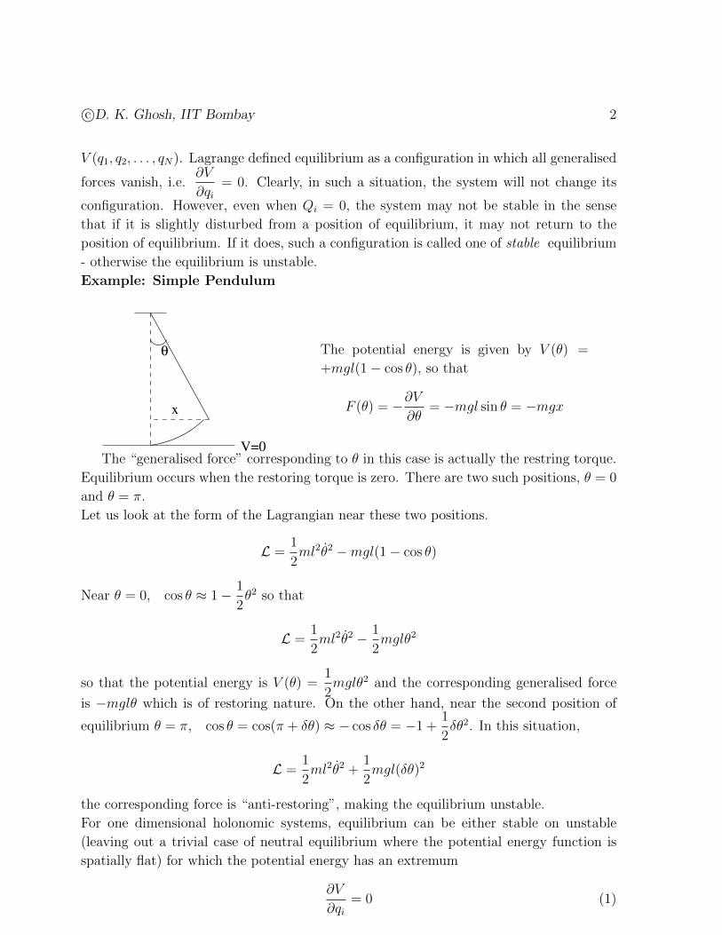
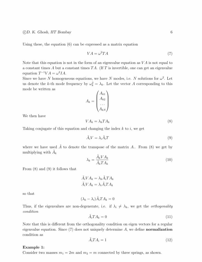
Consider two masses m1 = 2m and m2 = m connected by three springs, as shown.


k =

m

4kk =1

kk =2 2k

3

m 1 = 2m m2

=

We know that a single mass spring system with mass m and spring constant k has a

natural frequency of oscillation√k/m. Let us consider the system in the figure. Let the

generalised coordinates be displacement of the masses from their equilibrium positions,

the mass m1 being displaced by x1 while the mass m2 by an amount x2. The central

spring is then compressed or stretched by an amount x2−x1. Let us attempt to solve the

problem using the force method. The equations of motion for m1 and m2 are

m1x1 = −4kx1 − k(x1 − x2) (13a)

m2x2 = −2kx2 − k(x2 − x1) (13b)

The sign of the last term is fixed by taking x2 to be large positive so that the force on m1

is in the positive direction, as it ought to be.

We will attempt to solve this pair of coupled equations (13a) and (13b) by using a bit

of guesswork and a bit of luck. This will not work except in cases which show sufficient

symmetry. The idea is to find a linear combination of x1 and x2 so that the coupled

equations become uncoupled. Let us rewrite (13a) and (13b) as

2mx1 = −5kx1 + kx2 (14a)

mx2 = kx1 − 3kx2 (14b)

It can be easily seen that

m(x1 − x2) = −7

2k(x1 − x2) (15a)

m(2x2 + x1) = −2k(2x1 + x2) (15b)

Thus, if we define new normal coordinates

y1 = x1 − x2y2 = 2x1 + x2 (16)

the equations for y1 and y2 are uncoupled,

my1 = −7

2ky1

my2 = −2ky2 (17)

The normal coordinates oscillate with independent frequencies√

2k/m and√

7k/2m,

which are known as the normal modes. These new generalised coordinates execute


simple periodic oscillations known as normal oscillations. The new normal coordinates

satisfy

yα + ω2αyα = 0 (18)

With this intuitive background, let us look at the problem more formally.

The Lagrangian of the system is

L =1

2m1x

21 +

1

2m2x

22 −

1

2k1x

21 −

1

2k2(x2 − x1)2 −

1

2k3x

22 (19)

Define t and V matrices

t =∂2T

∂xi∂xj=

(m1 0

0 m2

)(20)

V =∂2V

∂xi∂xj=

(5k −k−k 3k

)(21)

Condition for existence of non-trivial solution is

det(Vik − ω2tik) = 0

which gives ∣∣∣∣5k − 2mω2 −k−k 3k −mω2

∣∣∣∣ = 0

which has the solution ω2 = 7k/2m and 2k/m. The normal modes are now found from

(6)

ω2TA = V A

Writing A =

(A1

A2

), we get, for ω2 =

7k

2m

7k

2m

(2m 0

0 m

)(A1

A2

)=

(5k −k−k 3k

)(A1

A2

)For this normal mode we have A2 = −2A1 so that (normalizing)

A =1√6m

(1

−2

)

For ω2 =2k

m, a similar calculation gives

A =1√3m

(1

1

)The general solution can then be written as(

x1x2

)= A

(1

1

)cosω−t+B

(1

1

)sinω−t+ C

(1

−2

)cosω+t+D

(1

−2

)sinω+t


We can fix the constants A,B,C and D by using initial conditions. Suppose we we pull

the two masses aside and release,

x1(0) = x10, x2(0) = x20, x1(0) = x2(0) = 0

we then have

A+ C = x10

A− 2C = x20

Bω− +Dω+ = 0

Bω− − 2Dω+ = 0

which gives

A =2

3x10 +

1

3x20

B = D = 0

C =1

3x10 −

1

3x20

so that

x1 =

(2

3x10 +

1

3x20

)cosω−t+

(1

3x10 −

1

3x20

)cosω+t (22)

x2 =

(2

3x10 +

1

3x20

)cosω−t−

(2

3x10 −

2

3x20

)cosω+t (23)

It can be checked that,

x1 − x2 = (x10 − x20) cosω+t

2x1 + x2 = (2x10 + x20) cosω−t

as expected.

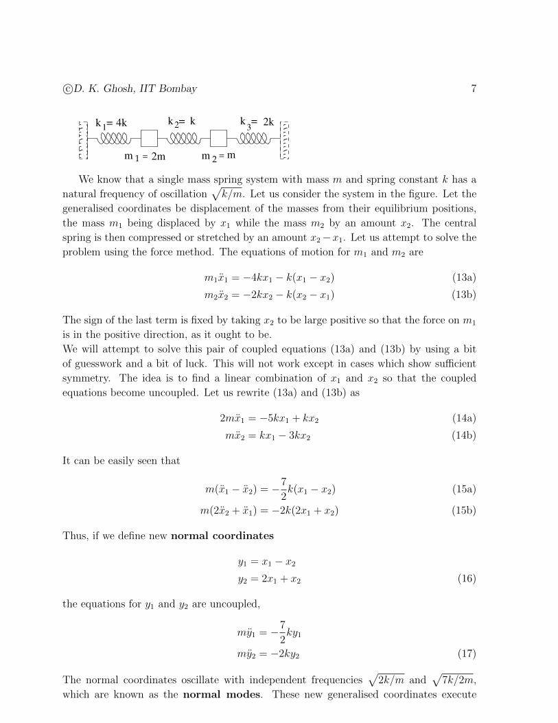
Example 2:

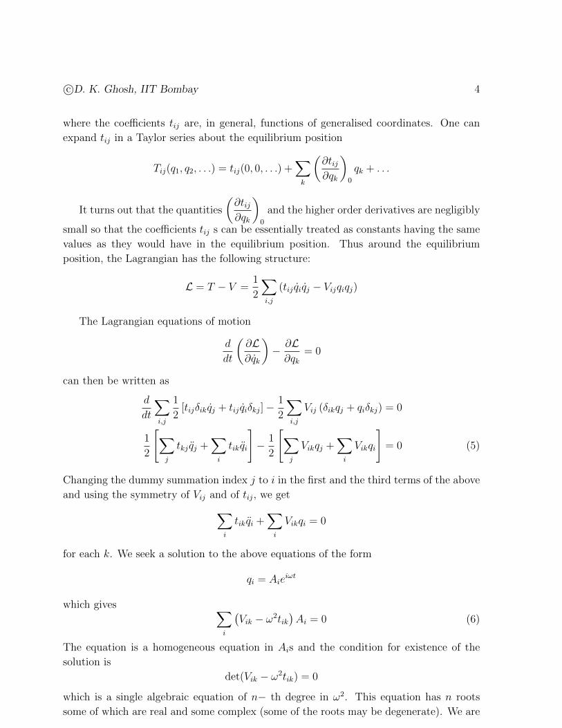
As a second example, consider a pair of identical pendulums consisting of a pair of mass-

less rigid rods of length l each at the end of each of which a mass m is attached. The

mid-points of the rods are connected by a spring of force constant k. In the absence of

coupling, each oscillator has a frequency ω =

√g

l. As before, let us try to solve the

problem by force method.

m m

A Be1 e2

k


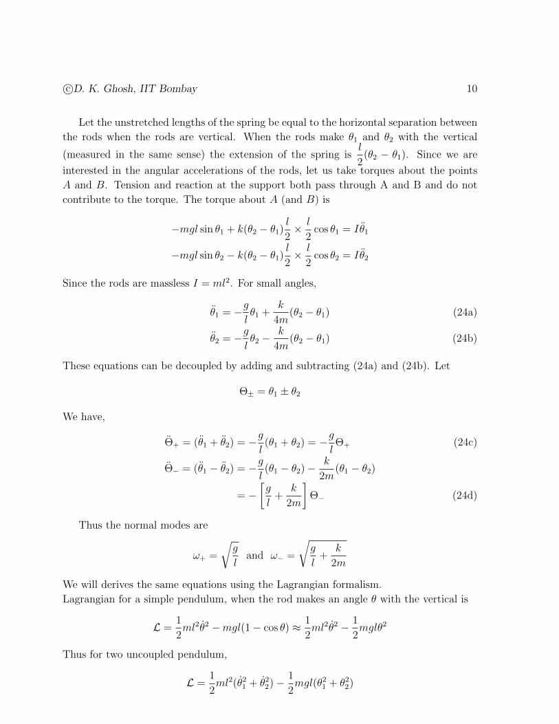
Let the unstretched lengths of the spring be equal to the horizontal separation between

the rods when the rods are vertical. When the rods make θ1 and θ2 with the vertical

(measured in the same sense) the extension of the spring isl

2(θ2 − θ1). Since we are

interested in the angular accelerations of the rods, let us take torques about the points

A and B. Tension and reaction at the support both pass through A and B and do not

contribute to the torque. The torque about A (and B) is

−mgl sin θ1 + k(θ2 − θ1)l

2× l

2cos θ1 = Iθ1

−mgl sin θ2 − k(θ2 − θ1)l

2× l

2cos θ2 = Iθ2

Since the rods are massless I = ml2. For small angles,

θ1 = −glθ1 +

k

4m(θ2 − θ1) (24a)

θ2 = −glθ2 −

k

4m(θ2 − θ1) (24b)

These equations can be decoupled by adding and subtracting (24a) and (24b). Let

Θ± = θ1 ± θ2

We have,

Θ+ = (θ1 + θ2) = −gl(θ1 + θ2) = −g

lΘ+ (24c)

Θ− = (θ1 − θ2) = −gl(θ1 − θ2)−

k

2m(θ1 − θ2)

= −[g

l+

k

2m

]Θ− (24d)

Thus the normal modes are

ω+ =

√g

land ω− =

√g

l+

k

2m

We will derives the same equations using the Lagrangian formalism.

Lagrangian for a simple pendulum, when the rod makes an angle θ with the vertical is

L =1

2ml2θ2 −mgl(1− cos θ) ≈ 1

2ml2θ2 − 1

2mglθ2

Thus for two uncoupled pendulum,

L =1

2ml2(θ21 + θ22)−

1

2mgl(θ21 + θ22)


Additional potential energy due to the spring is1

2k

(l

2

)2

(θ2−θ1)2. Thus the Lagrangian

for the coupled pendulum is

L =1

2ml2(θ21 + θ22)−

1

2mgl(θ21 + θ22)−

1

8kl2(θ2 − θ1)2 (25)

[We can derive (24a) and (24b) using the Euler-Lagrange equations corresponding to θ1and θ2.] The t and V matrices are

t =

(ml2 0

0 ml2

)(26)

V =

mgl +kl2

4−kl

2

4

−kl2

4mgl +

kl2

4

(27)

The secular equation is

det | V − ω2t |= 0

which gives ∣∣∣∣∣∣∣mgl +

kl2

4− ω2ml2 −kl

2

4

−kl2

4mgl +

kl2

4− ω2ml2

∣∣∣∣∣∣∣ = 0

which has solutions ω2 =g

l(≡ ω2

+) andg

l+

k

2m(≡ ω2

−). Let us look at the coordinates

when the frequency equals one of the normal mode frequencies. Let us rewrite (24a) and

(24b)

−ω2θ1 = −glθ1 +

k

4m(θ2 − θ1) (28a)

ω2θ2 = −glθ2 −

k

4m(θ2 − θ1) (28b)

which can be written in matrix form as−ω2 +g

l+

k

4m− k

4m

− k

4m−ω2 +

g

l+

k

4m

(θ1θ2

)= 0

For ω = ω+, this gives θ1 = θ2, so that the mode is a symmetric mode having the following

solution for the mode coordinate.

θ+ = A+ cos(ω+t+ δ+) (29)

For ω = ω−, the mode is antisymmetric with θ2 = −θ1 and the normal coordinate is

θ− = A− cos(ω−t+ δ−) (30)


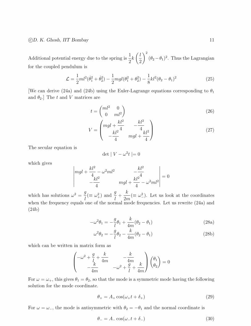
The constants A+, A−, δ+ and δ− are fixed from initial conditions. When the system

is in the symmetric mode, the two pendulums move in phase while when they are in the

antisymmetric mode they are out of phase by π.

m m

A Be

k

mm

ee e

Anti− symmetric mode Symmetric Mode

We can combine the two modes to get solutions for θ1 and θ2,

θ1 =A+

2cos(ω+t+ δ+) +

A−

2cos(ω−t+ δ−) (31a)

θ2 =A+

2cos(ω+t+ δ+)− A−

2cos(ω−t+ δ−) (31b)

Suppose the two pendula are both pulled aside by θ0 and released. We then have A− = 0.

We then have

θ1 = θ2 =A+

2cos(ω+t+ δ+)

which shows that the system always remains in the symmetric mode.

Except when the system is in a single mode, there is transfer of energy between the two

modes at a frequency known as the beat frequency. When the two modes are present

with the same strength, for instances when only one of the pendula is drawn aside and

released initially, we can take A− = A+ = A and δ+ = δ− = 0. In this case, θ1 = A and

θ2 = 0 at t = 0. The expressionds for θ1 and θ2 are given by

θ1 = A cos(ω+t) + A cos(ω−t)

θ2 = A cos(ω+t)− A cos(ω−t)

so that

θ+ = θ1 + θ2 = 2A cos(ω+t)

θ− = θ1 − θ2 = 2A cos(ω−t)

We can rewrite the aboves as

θ1 = 2A cos(ω+ − ω−

2t) cos(

ω+ + ω−

2t)

θ2 = 2A sin(ω+ − ω−

2t) sin(

ω+ + ω−

2t)


Define beat frequency ωb and the average frequency ω as

ωb =ω+ − ω−

2and ω =

ω+ + ω−

2

in terms of which

θ1 = 2A cos(ωbt) cos(ωt)

θ2 = 2A sin(ωbt) sin(ωt)

For weak couplings ωb ω. After a time t =π

2ωb, we have θ1 = 0 and θ2 = 2A sinωt,

i.e. the first pendulum has momentarily stopped and all the energy has been transferred

to the second.

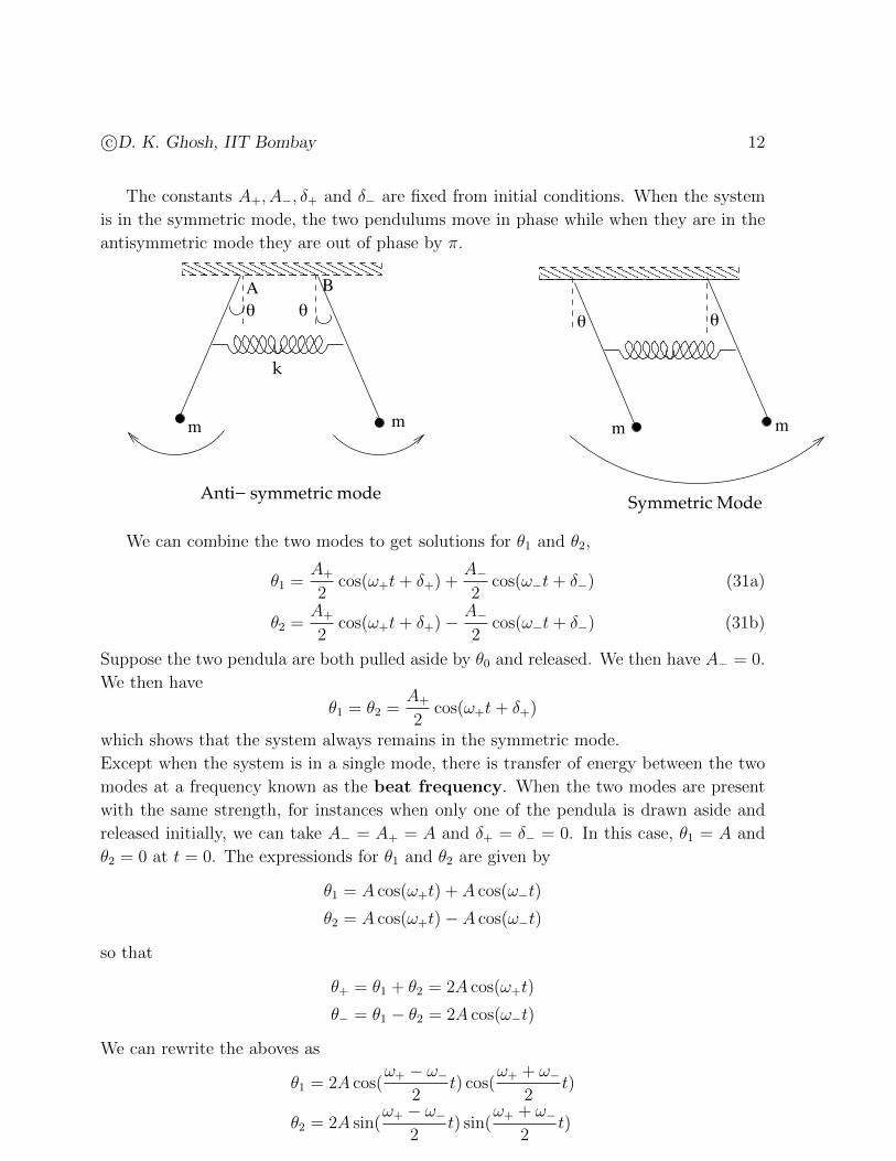
Example 3: Normal Modes of a Triatomic Molecule

Molecules like CO2 have linear structures (O−−−C−−−O) with two equal masses

m at either ends and a central mass M . These are modelled through the three masses

connected by two identical springs, as shown in the figure. Clearly, there are three normal

modes – one when all the three masses move in unison, a second where the end masses

move in opposite directions while the central mass remains at rest and a third where the

two end masses move in opposite directions while the central mass moves towards the

mass moving towards it.

k k

m mM

The Lagrangian is written as

L =1

2m(x21 + x23) +

1

2Mx22 −

k

2

[(x2 − x1)2 + (x3 − x1)2

]The matrices T and V are as follows

V =

k −k 0

−k 2k −k0 −k k

T =

m 0 0

0 M 0

0 0 m


The secular equation is det(V − ω2T ) = 0, which gives∣∣∣∣∣∣k − ω2m −k 0

−k 2k − ω2M −k0 −k k − ω2

∣∣∣∣∣∣ = 0

which has the solutions ω = ω1, ω2, ω3, where

ω21 = 0

ω22 =

k

m

ω23 =

k

m+

2k

M

1. For ω = 0, the equation (8) V A− ω2TA = 0 can be written as k −k 0

−k 2k −k0 −k k

A1

A2

A3

= 0

which gives A1 = A2 = A3. Taking each of them to be equal to 1 (in some unit) we

get

A =1√N

1

1

1

where N is to be fixed by normalization. Normalization condition gives

1

N

(1 1 1

)m 0 0

0 M 0

0 0 m

1

1

1

= 1

i.e. M + 2m = N . Thus the normalized vector is

1√2m+M

1

1

1

(32)

As expected, the displacement of each mass is the same and the masses move in

unision.

2. Consider ω2 =k

m. For this case, we have

0 −k 0

−k k −k0 −k 0

A1

A2

A3

= 0


which gives A2 = 0 and A1 = A3. Using the orthogonality with the mode ω1, we

take this mode to be

1√N

1

0

−1

Normalization condition fixes N = 2m and the displacement vector is

1√2m

1

0

−1

which shows the central mass to be at rest while the end masses displace by the

same amount in the opposite direction.

3. For ω2 =k

m+

2k

M, the equation is

−2

km

M−k 0

−k −kMm

−k

0 −k −2km

M

A1

A2

A3

= 0

which gives A1 = A3 and A2 = −2m

MA1. The normalization can be done as in the

previous cases. The displacement vector is given by

√M

2mM + 4m2

1

−2m/M

1

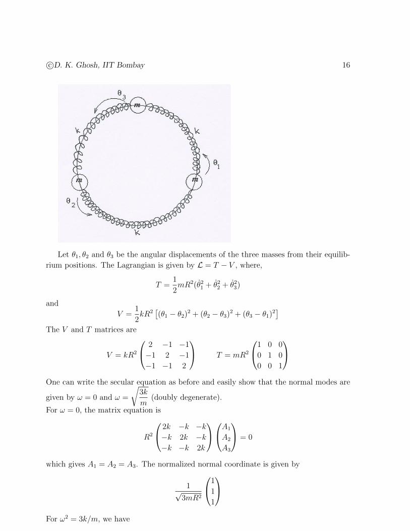
Example 4

Three masses m each, initially located equidistant from one another on a horizontal circle

of radius R. They are connected in pairs by three springs of force constant k each and

of unstretched length 2πR/3. The spring threads the circuloar tract so that the mass is

constrained to move on the circle. Find the normal modes.


Let θ1, θ2 and θ3 be the angular displacements of the three masses from their equilib-

rium positions. The Lagrangian is given by L = T − V , where,

T =1

2mR2(θ21 + θ22 + θ23)

and

V =1

2kR2

[(θ1 − θ2)2 + (θ2 − θ3)2 + (θ3 − θ1)2

]The V and T matrices are

V = kR2

2 −1 −1

−1 2 −1

−1 −1 2

T = mR2

1 0 0

0 1 0

0 0 1

One can write the secular equation as before and easily show that the normal modes are

given by ω = 0 and ω =

√3k

m(doubly degenerate).

For ω = 0, the matrix equation is

R2

2k −k −k−k 2k −k−k −k 2k

A1

A2

A3

= 0

which gives A1 = A2 = A3. The normalized normal coordinate is given by

1√3mR2

1

1

1

For ω2 = 3k/m, we have


−k −k −k−k −k −k−k −k −k

A1

A2

A3

= 0

which gives A1 +A2 +A3 = 0. The eigenvectors cannot be uniquely fixed. However, if we

use the orthogonality with the zero mode, we can have the following (non-unique) choices:

1√6mR2

2

−1

−1

and

1√2mR2

0

1

−1

3 Damped and Forced Oscillations

3.1 Rayleigh Disspipation Function

We have seen that for systems where forces are derivable from a potential, Euler-Lagrange

equation is given byd

dt

(∂L∂qi

)− ∂L∂qi

= 0

This was seen to be true even when a velocity dependent potential exists, as was in the

case of Lorentz force. If on the otrher hand, there are some non-potential forces Qi, we

get, using the same procedure as was used to derive the Euler-Lagrange equation from

d’Alembert’s principle,

d

dt

(∂L∂qi

)− ∂L∂qi

= Qi

where Qi =∑

j~Fj ·

∂~rj∂qi

. Example of a non-potential force is frictional force which, in most

cases of interest, is proportional to the velocity of the particle, and, is given by ~F = −k~v.

More generally, the form of the frictional force is

~F = −kxvxi− kyvy j − kzvzk

where kx, ky and kz are all positive constants. One can include such non-potential forces

in the Lagrangian formalism by defining Rayleigh Dissipation Function R,

R =1

2

∑i

(kxv2x + kyv

2y + kzv

2z) (33)


The force ~Fi is then given by

Fix = − ∂R∂vix

i.e.~Fi = −∇viR

where the gradient is taken with respect to velocity field and the index i is the particle

index. Work done by the system in overcoming resistive force is

dW = −~F · d~r = −~F · ~vdt = −2Rdt

so that

dW

dt= −2R (34)

The generalized force can be written as

Qi =∑j

~Fj ·∂~rj∂qi

=∑j

~Fj ·∂~rj∂qi

= −∑j

∇vjR ·∂~rj∂qi

= −∂R∂qi

(35)

where in the second step of the above equation we have used the “dot cancellation”. Thus

we can use this term in the Euler Lagrange equation by incorporating an additional term

d

dt

(∂L∂qi

)− ∂L∂qi

+∂R∂qi

= Qi (36)

where Qi are non-potential forces which are not derivable either from a potential or from

a dissipation function.

3.2 Damped Oscillator

Consider a linear oscillator with dissipative force proportional to the velocity. Taking

Rayleigh function to be R = αq2 and using the Lagrangian L =1

2mq2 − 1

2kq2, we get

from the modified Euler Lagrange equation (36)

mq + 2αq + kq = 0


Defining ω0 =

√k

mand γ =

α

m, the get the equation for the damped oscillator to be

given by

q + 2γq + ω20 = 0 (37)

We seek solution of the form q = q0eλt which gives

dq

dt= q0λe

λt andd2q

dt2= q0λ

2eλt.

Substituting these in (37), we get

λ2 + 2γλ+ ω20 = 0 (38)

which has the solution

λ = −γ ±√γ2 − ω2

0

Thus the solution of (37) is

q = e−γt[Ae√γ2−ω2

0t +Be−√γ2−ω2

0t]

(39)

Let us consider some special cases.

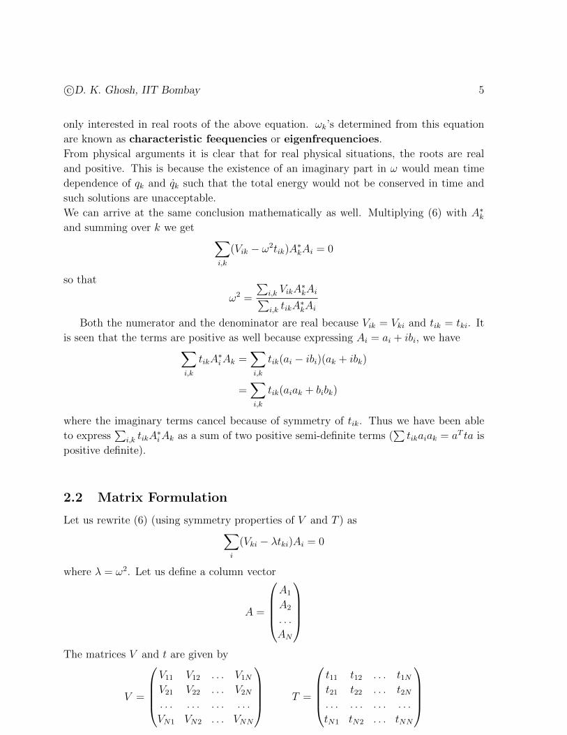
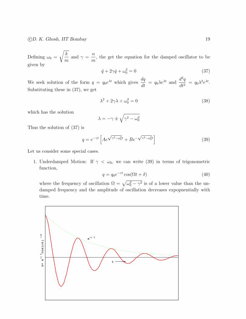
1. Underdamped Motion: If γ < ω0, we can write (39) in terms of trigonometric

function,

q = q0e−γt cos(Ωt+ δ) (40)

where the frequency of oscillation Ω =√ω20 − γ2 is of a lower value than the un-

damped frequency and the amplitude of oscillation decreases expopnentially with

time.

x= e-a tcos(tt)

t

e-a t


The energy of the oscillator decreases in the presence of dissipative forces. Using

E =∂L∂qq − L we get

dE

dt=

d

dt

(∂L∂qq

)− dLdt

=d

dt

(∂L∂q

)q +

∂L∂qq −

(∂L∂qq +

∂L∂qq

)= −∂R

∂qq

= −2R

where we have used (36) and (34) in the last step. Since R > 0, there is always a

dissipation of energy.

2. Overdamped Motion : If γ > ω0, the solution is of the form

q(t) = Ae−γ1t +Be−γ2t

where γ1,2 = γ ∓√γ2 − ω2

0 are both positive. and the oscillation dies off fast.

3. Critical Damping : Critical damping occurs when the roots of the characterisatic

equation becomes equal, i.e., when ω0 = γ = −λ. In such a case the two constants

A and B in (39) becomes a single constant C. However, as we have a second order

differential equation, we must have two constants. Let us try a solution of the form

q(t) = u(t)eλt. We then have

dq

dt=du

dteλt + uλeλt

dq

dt2= eλt

(d2u

dt2+ 2λ

du

dt+ λ2

)Substituting this in the differential equation q + 2γq + ω2

0q = 0, we get

d2u

dt2+ 2(λ+ γ)

du

dt+ (λ2 + 2γλ+ ω2

0)u = 0

However, λ being a root of the characteristic equation, we have λ2+2γλ+ω20 = 0. In

addition, we are looking for the situation where λ = −γ. Thus we get d2u/dt2 = 0,

which has the solution u(t) = A+Bt. The solution for q is

q = (A+Bt)e−γt

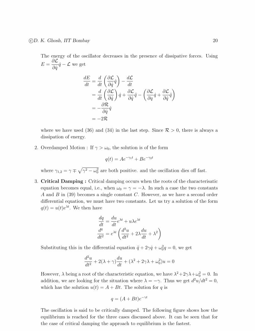
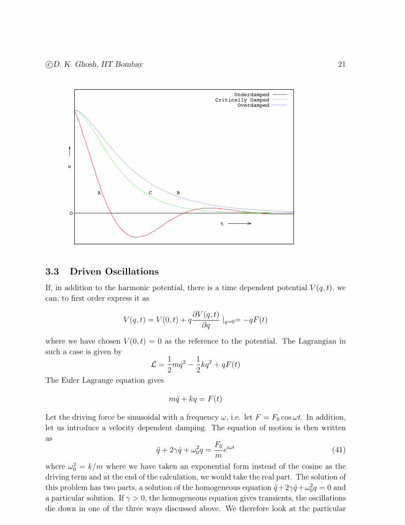
The oscillation is said to be critically damped. The following figure shows how the

equilibrium is reached for the three cases discussed above. It can be seen that for

the case of critical damping the approach to equilibrium is the fastest.

c©D. K. Ghosh, IIT Bombay 21x

t

A BC

O

UnderdampedCritically Damped

Overdamped

3.3 Driven Oscillations

If, in addition to the harmonic potential, there is a time dependent potential V (q, t), we

can, to first order express it as

V (q, t) = V (0, t) + q∂V (q, t)

∂q|q=0= −qF (t)

where we have chosen V (0, t) = 0 as the reference to the potential. The Lagrangian in

such a case is given by

L =1

2mq2 − 1

2kq2 + qF (t)

The Euler Lagrange equation gives

mq + kq = F (t)

Let the driving force be sinusoidal with a frequency ω, i.e. let F = F0 cosωt. In addition,

let us introduce a velocity dependent damping. The equation of motion is then written

as

q + 2γq + ω20q =

F0

meiωt (41)

where ω20 = k/m where we have taken an exponential form instead of the cosine as the

driving term and at the end of the calculation, we would take the real part. The solution of

this problem has two parts, a solution of the homogeneous equation q+2γq+ω20q = 0 and

a particular solution. If γ > 0, the homogeneous equation gives transients, the oscillations

die down in one of the three ways discussed above. We therefore look at the particular


solution. The equation is solved by an ansatz q = Ae−iωt which gives q = −iωq and

q = −ω2q. Substituting these in the differential equation (41), we get

(−ω2 − 2iωγ + ω20)Ae−iωt =

F0

me−iωt

We then have

A =F0

m

1

ω20 − ω2 − 2iωγ

so that

q = <(F0

m

1

ω20 − ω2 − 2iωγ

e−iωt)

We then have

A =F0/m√

(ω20 − ω2)2 + 4ω2γ2

e−iϕ

where the phase ϕ is given by

ϕ = tan−1

(2ωγ

ω2 − ω20

)Thus we can write q as

q =| A | cos(ωt+ ϕ)

Using the expression for tanϕ, we get

cosϕ =ω2 − ω2

0√(ω2

0 − ω2)2 + 4ω2γ2

sinϕ =2ωγ√

(ω20 − ω2)2 + 4ω2γ2

The motion is oscillatory with the frequency same as that of the driving frequency.

As the strength of damping decreases, the amplitude A gets peaked when the driving

frequency becomes equal to the natural frequency ω0. For values of driving frequencies

well below that of natural frequency, the response of the oscillator is in phase with the

driving frequency (sinϕ → 0 =⇒ ϕ → 0). Near resonant frequency, sinϕ ≈ 1, i.e.

ϕ = π/2. For ω ω0, sinϕ→ 0 but cosϕ→ −1, i.e. it becomes in anti-phase.

The energy loss of a weakly damped oscillator is characterized by Q-factor which is

defined as 2π times the energy stored in the oscillator divided by the energy loss in one

period. It can be shown that near resonance Q =ω0

2γ. Thus a sharp resonance results in

a high Q value.

Classical Mechanics Small Oscillations

Documents