Classical eld techniques for nite temperature Bose gases · Classical eld techniques for nite temperature Bose gases N 0 N /N = 0.02 0 N /N = 0.45 0 /N = 0.93 Matthew Davis ARC Centre

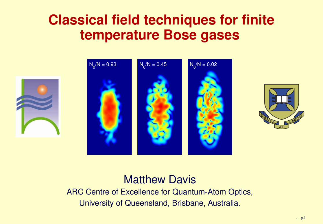
Classical field techniques for finitetemperature Bose gases

N0/N = 0.02N0/N = 0.45N0/N = 0.93

Matthew DavisARC Centre of Excellence for Quantum-Atom Optics,

University of Queensland, Brisbane, Australia.. – p.1

Australian Centre for Quantum-Atom Opticswww.acqao.org

One of eight Australian Centre’s of Excellence funded in 2004.

Australian National University (Canberra):— Rb BEC and atom laser, He∗ BEC, atom-light entanglement,quantum imaging, theory.

Swinburne University of Technology (Melbourne):— Rb BEC on atom chip, quantum degenerate Fermi gas.

University of Queensland (Brisbane):— Main theory node: quantum dynamics and correlations.

. – p.2

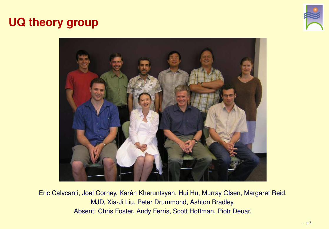
UQ theory group

Eric Calvcanti, Joel Corney, Karen Kheruntsyan, Hui Hu, Murray Olsen, Margaret Reid.MJD, Xia-Ji Liu, Peter Drummond, Ashton Bradley.

Absent: Chris Foster, Andy Ferris, Scott Hoffman, Piotr Deuar.. – p.3

Overview

• Finite temperature Bose gases.• Introduction to classical fields.• Simulation of classical fields.• Application: Shift in Tc for interacting Bose gases.• Quantum dynamics with classical fields.

. – p.4

The challenge for theoristsCan we come up with a practical non-equilibriumformalism for finite temperature Bose gases?

Desirable features:•• Can deal with inhomogeneous potentials.• Can treat interactions non-perturbatively.• Calculations can be performed on a reasonable time

scale (say under one week).

. – p.5

Potential applicationsTopics of interest include:

• Condensate formation.• Vortex lattice formation and dynamics.• Low dimensional systems (fluctuations important).• Correlations.• Heating effects.• Atom lasers . . .

. – p.6

Classical fields for matter waves

. – p.7

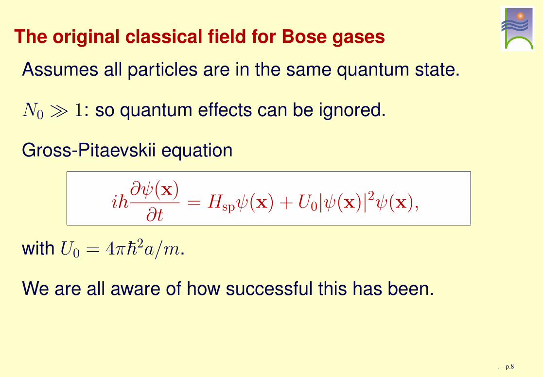
The original classical field for Bose gasesAssumes all particles are in the same quantum state.

N0 � 1: so quantum effects can be ignored.

Gross-Pitaevskii equation

i~∂ψ(x)

∂t= Hspψ(x) + U0|ψ(x)|2ψ(x),

with U0 = 4π~2a/m.

We are all aware of how successful this has been.

. – p.8

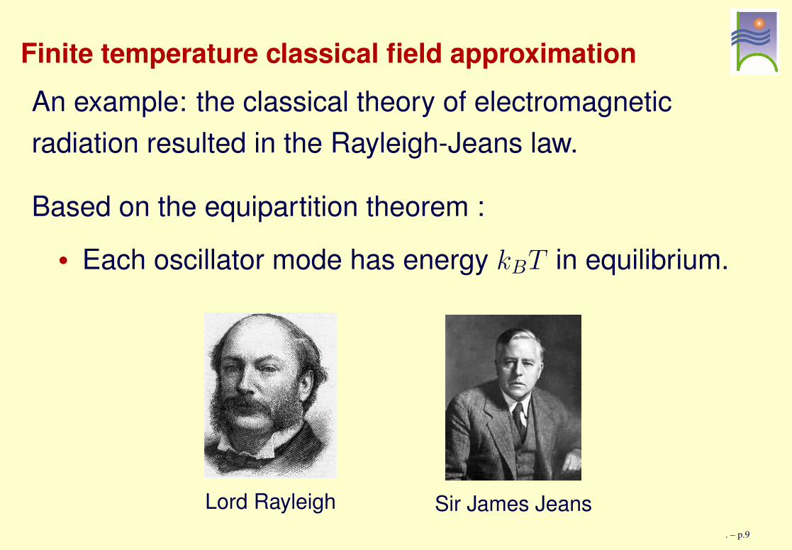
Finite temperature classical field approximationAn example: the classical theory of electromagneticradiation resulted in the Rayleigh-Jeans law.

Based on the equipartition theorem :• Each oscillator mode has energy kBT in equilibrium.

Lord Rayleigh Sir James Jeans. – p.9

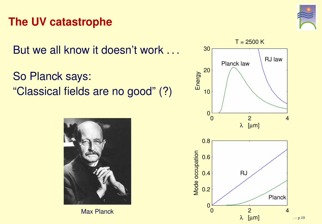
The UV catastrophe

But we all know it doesn’t work . . .

So Planck says:“Classical fields are no good” (?)

Max Planck

0 2 40

10

20

30

λ [µm]

Ener

gy

RJ lawPlanck law

T = 2500 K

0 2 40

0.2

0.4

0.6

0.8

λ [µm]

Mod

e oc

cupa

tion

RJ

Planck

. – p.10

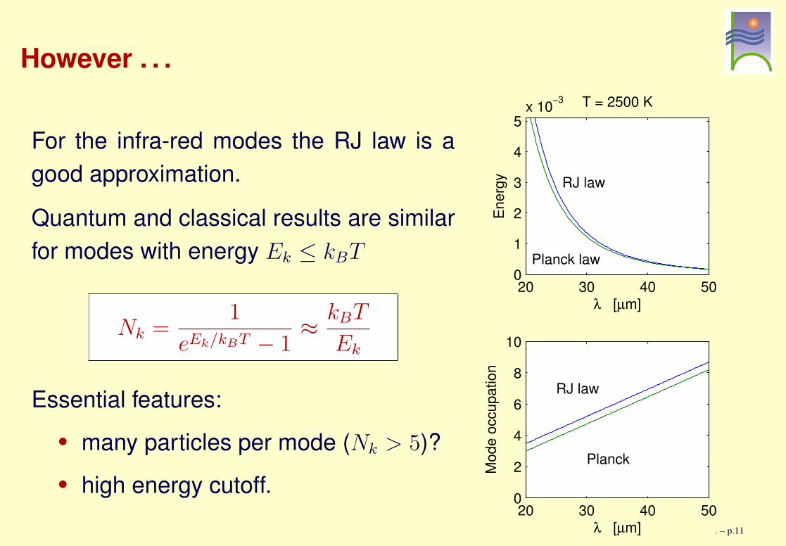
However . . .

For the infra-red modes the RJ law is agood approximation.

Quantum and classical results are similarfor modes with energy Ek ≤ kBT

Nk =1

eEk/kBT − 1≈ kBT

Ek

Essential features:• many particles per mode (Nk > 5)?• high energy cutoff.

20 30 40 500

1

2

3

4

5x 10−3

λ [µm]

Ener

gy

Planck law

RJ law

T = 2500 K

20 30 40 500

2

4

6

8

10

λ [µm]

Mod

e oc

cupa

tion

RJ law

Planck

. – p.11

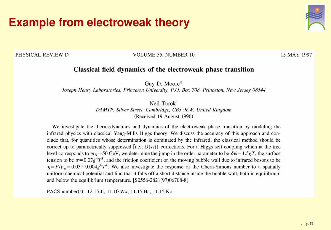
Example from electroweak theory

. – p.12

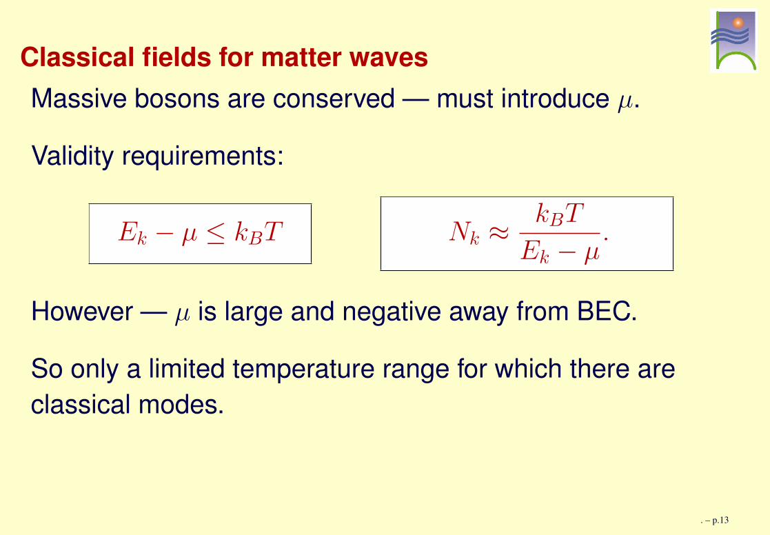
Classical fields for matter wavesMassive bosons are conserved — must introduce µ.

Validity requirements:

Ek − µ ≤ kBT Nk ≈kBT

Ek − µ.

However — µ is large and negative away from BEC.

So only a limited temperature range for which there areclassical modes.

. – p.13

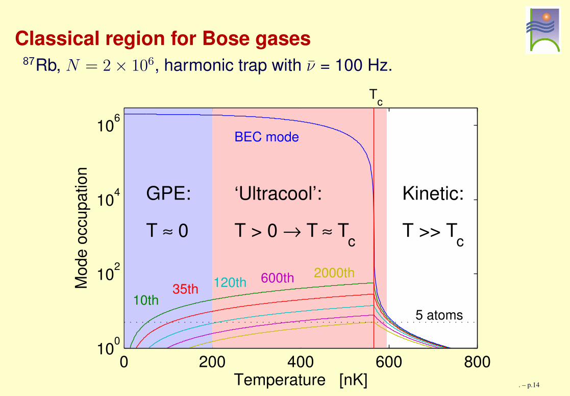
Classical region for Bose gases87Rb, N = 2 × 106, harmonic trap with ν = 100 Hz.

0 200 400 600 800100

102

104

106

TcM

ode

occu

patio

n

Temperature [nK]

GPE:

T ≈ 0

‘Ultracool’:

T > 0 → T ≈ Tc

Kinetic:

T >> Tc

5 atoms

BEC mode

10th35th 120th 600th 2000th

. – p.14

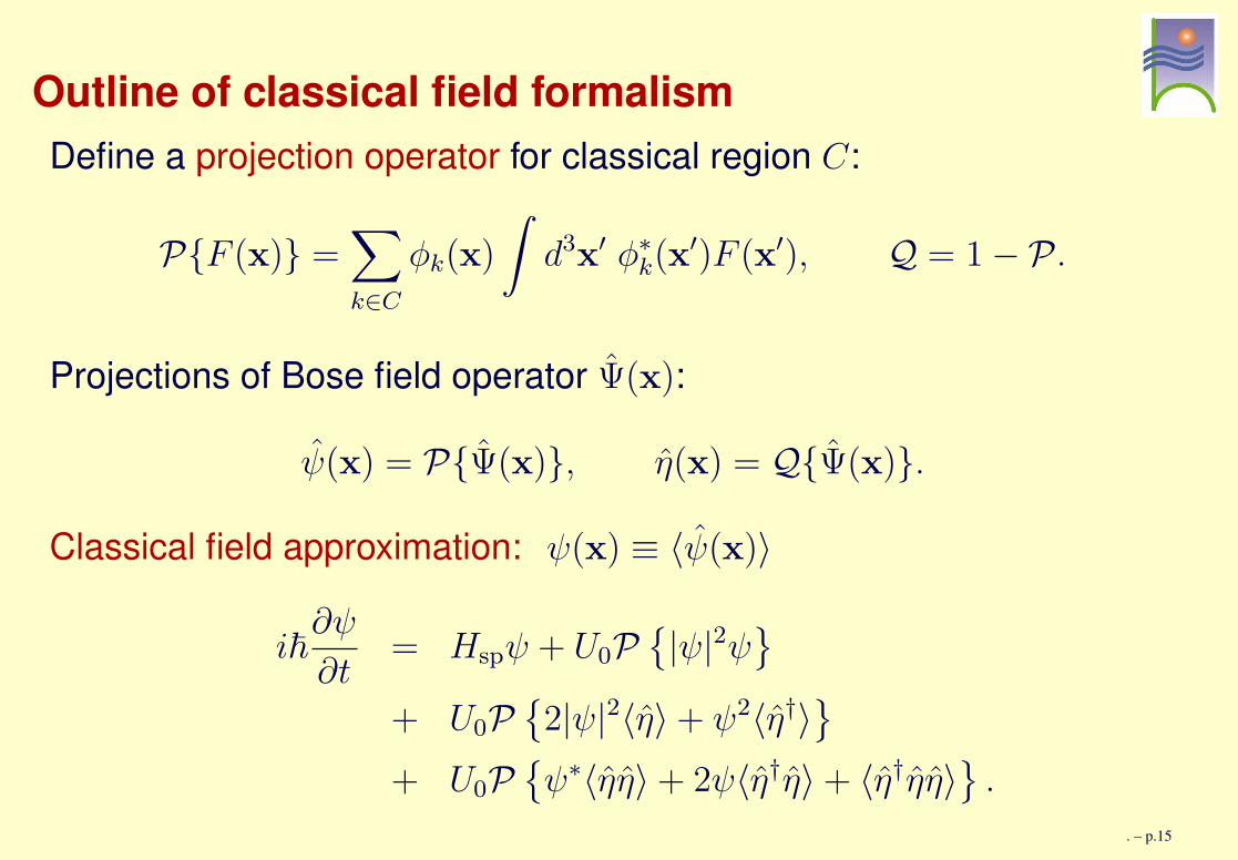
Outline of classical field formalismDefine a projection operator for classical region C:

P{F (x)} =∑

k∈C

φk(x)

∫

d3x′ φ∗

k(x′)F (x′), Q = 1 − P .

Projections of Bose field operator Ψ(x):

ψ(x) = P{Ψ(x)}, η(x) = Q{Ψ(x)}.

Classical field approximation: ψ(x) ≡ 〈ψ(x)〉

i~∂ψ

∂t= Hspψ + U0P

{

|ψ|2ψ}

+ U0P{

2|ψ|2〈η〉 + ψ2〈η†〉}

+ U0P{

ψ∗〈ηη〉 + 2ψ〈η†η〉 + 〈η†ηη〉}

.

. – p.15

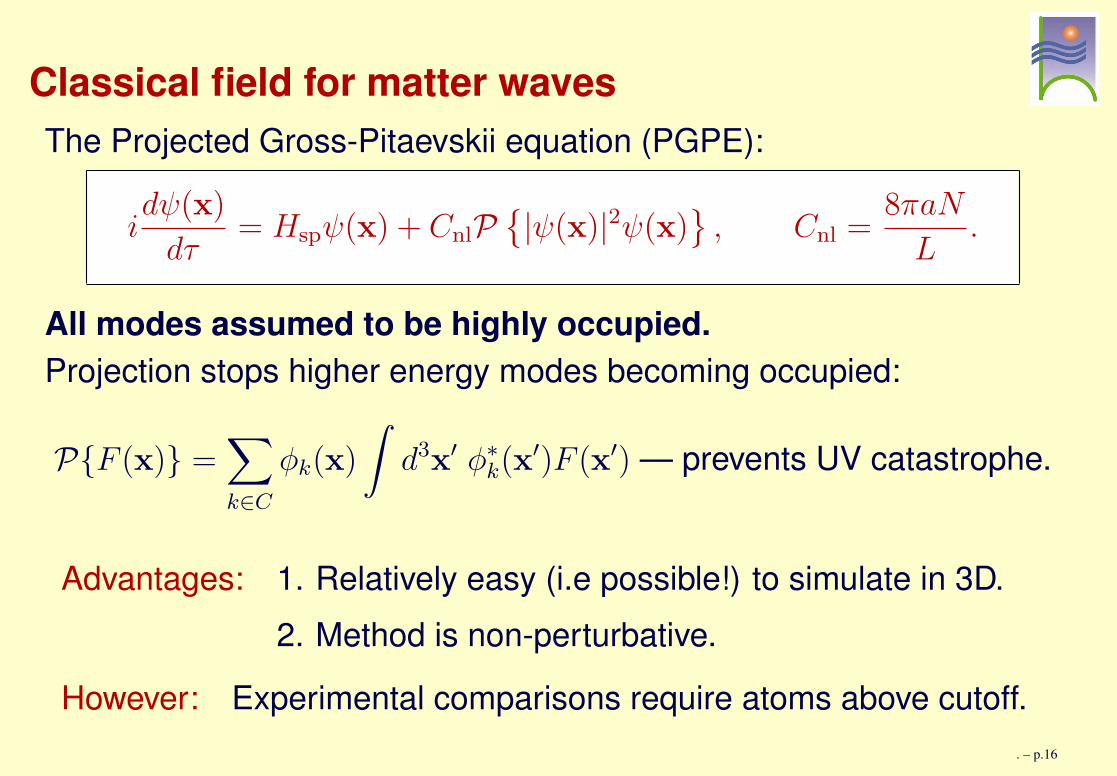
Classical field for matter wavesThe Projected Gross-Pitaevskii equation (PGPE):

idψ(x)

dτ= Hspψ(x) + CnlP

{

|ψ(x)|2ψ(x)}

, Cnl =8πaN

L.

All modes assumed to be highly occupied.Projection stops higher energy modes becoming occupied:

P{F (x)} =∑

k∈C

φk(x)

∫

d3x′ φ∗

k(x′)F (x′) — prevents UV catastrophe.

Advantages: 1. Relatively easy (i.e possible!) to simulate in 3D.2. Method is non-perturbative.

However: Experimental comparisons require atoms above cutoff.. – p.16

Classical field simulations

. – p.17

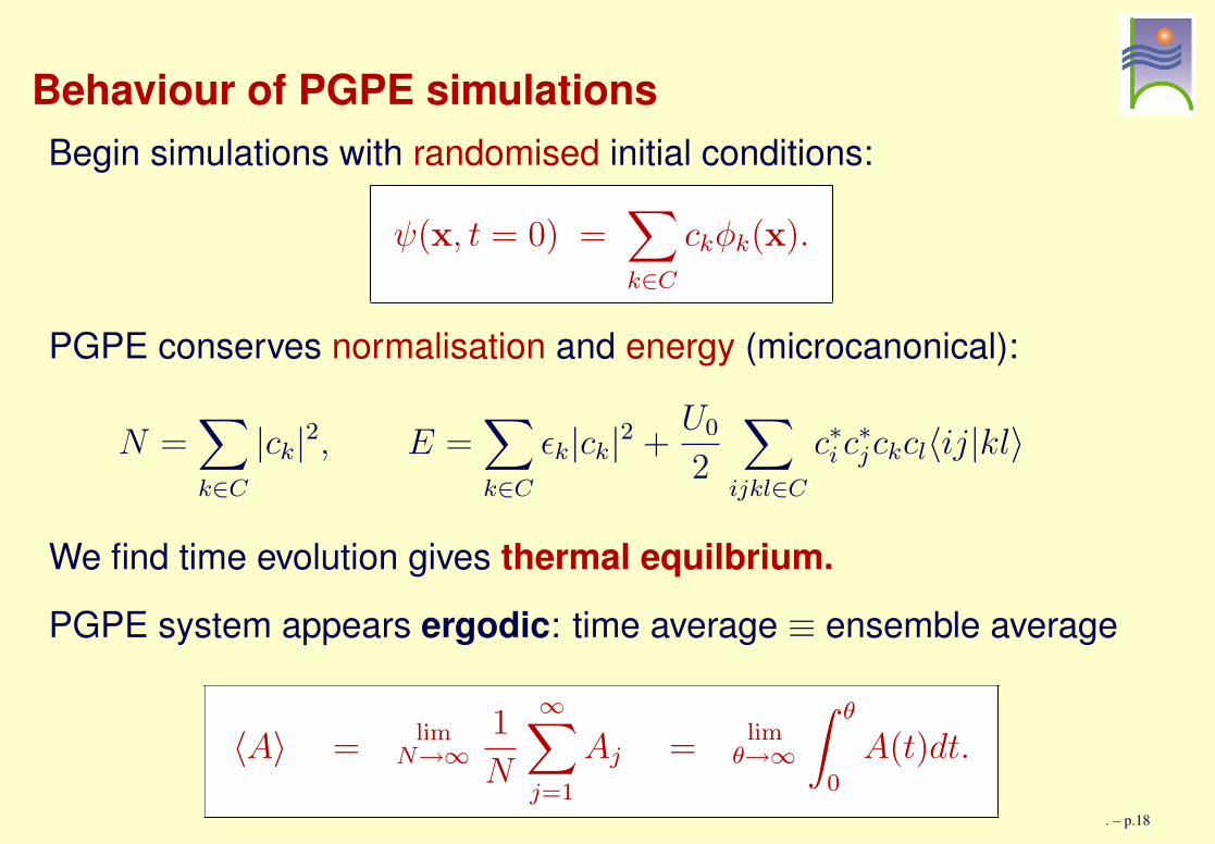
Behaviour of PGPE simulationsBegin simulations with randomised initial conditions:

ψ(x, t = 0) =∑

k∈C

ckφk(x).

PGPE conserves normalisation and energy (microcanonical):

N =∑

k∈C

|ck|2, E =∑

k∈C

εk|ck|2 +U0

2

∑

ijkl∈C

c∗i c∗jckcl〈ij|kl〉

We find time evolution gives thermal equilbrium.

PGPE system appears ergodic: time average ≡ ensemble average

〈A〉 =lim

N→∞

1

N

∞∑

j=1

Aj =lim

θ→∞

∫ θ

0

A(t)dt.

. – p.18

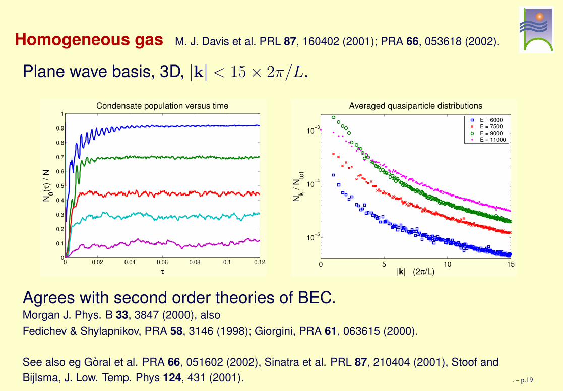
Homogeneous gas M. J. Davis et al. PRL 87, 160402 (2001); PRA 66, 053618 (2002).

Plane wave basis, 3D, |k| < 15 × 2π/L.

0 0.02 0.04 0.06 0.08 0.1 0.120

0.1

0.2

0.3

0.4

0.5

0.6

0.7

0.8

0.9

1Condensate population versus time

τ

N 0(τ) /

N

0 5 10 15

10−5

10−4

10−3

|k| (2π/L)

N k / N to

t

Averaged quasiparticle distributionsE = 6000E = 7500E = 9000E = 11000

Agrees with second order theories of BEC.Morgan J. Phys. B 33, 3847 (2000), alsoFedichev & Shylapnikov, PRA 58, 3146 (1998); Giorgini, PRA 61, 063615 (2000).

See also eg Goral et al. PRA 66, 051602 (2002), Sinatra et al. PRL 87, 210404 (2001), Stoof andBijlsma, J. Low. Temp. Phys 124, 431 (2001). . – p.19

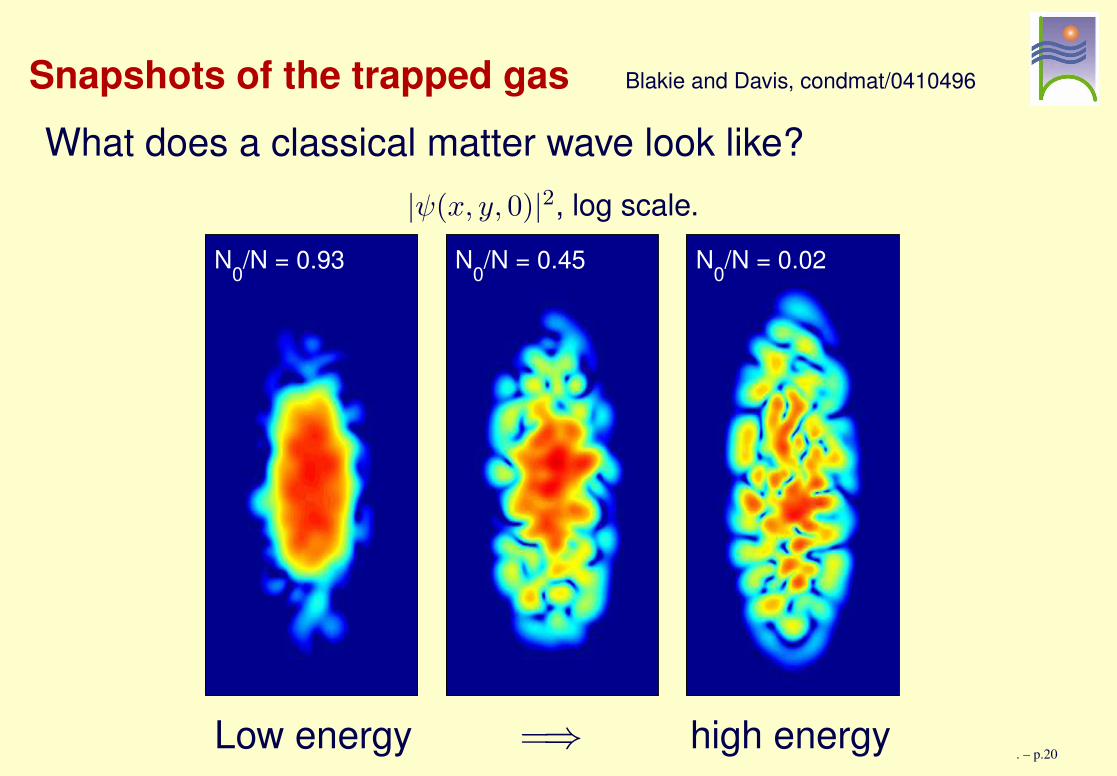
Snapshots of the trapped gas Blakie and Davis, condmat/0410496

What does a classical matter wave look like?|ψ(x, y, 0)|2, log scale.

N0/N = 0.02N0/N = 0.45N0/N = 0.93

Low energy =⇒ high energy. – p.20

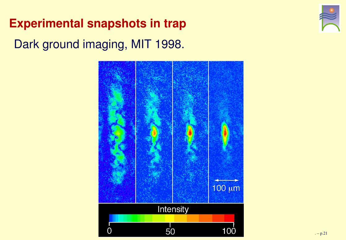
Experimental snapshots in trapDark ground imaging, MIT 1998.

. – p.21

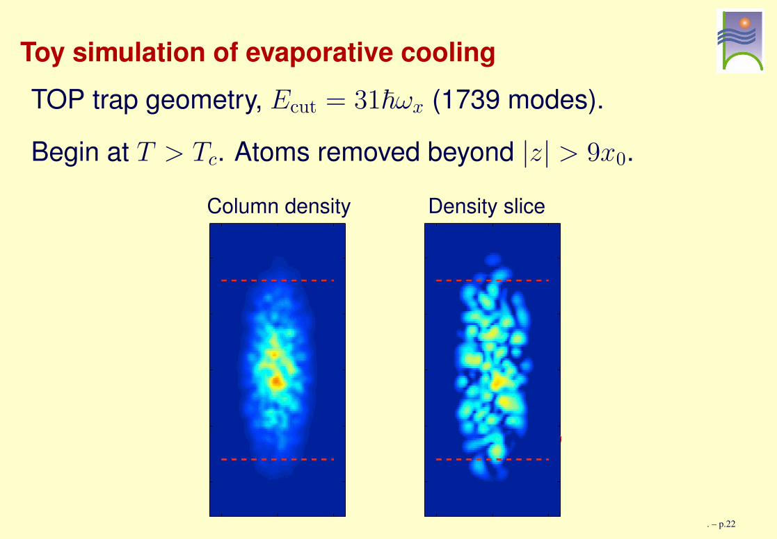
Toy simulation of evaporative coolingTOP trap geometry, Ecut = 31~ωx (1739 modes).

Begin at T > Tc. Atoms removed beyond |z| > 9x0.

Column density Density slice

. – p.22

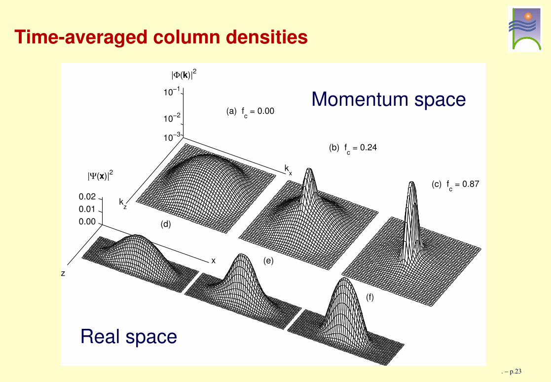
Time-averaged column densities

(c) fc = 0.87

(f)

(b) fc = 0.24

kx

(e)

(a) fc = 0.00

x

|Φ(k)|2

10−3

10−2

10−1

(d)

kz

|Ψ(x)|2

0.000.010.02

z

Momentum space

Real space. – p.23

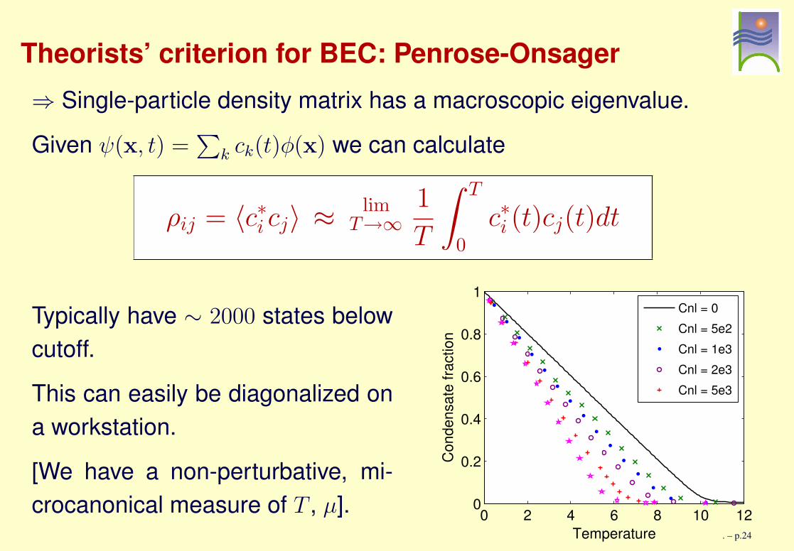
Theorists’ criterion for BEC: Penrose-Onsager⇒ Single-particle density matrix has a macroscopic eigenvalue.

Given ψ(x, t) =∑

k ck(t)φ(x) we can calculate

ρij = 〈c∗i cj〉 ≈ limT→∞

1

T

∫ T

0

c∗i (t)cj(t)dt

Typically have ∼ 2000 states belowcutoff.

This can easily be diagonalized ona workstation.

[We have a non-perturbative, mi-crocanonical measure of T , µ]. 0 2 4 6 8 10 12

0

0.2

0.4

0.6

0.8

1

Temperature

Cond

ensa

te fr

actio

n

Cnl = 0Cnl = 5e2Cnl = 1e3Cnl = 2e3Cnl = 5e3

. – p.24

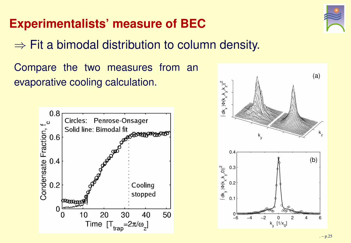
Experimentalists’ measure of BEC⇒ Fit a bimodal distribution to column density.Compare the two measures from anevaporative cooling calculation.

−6 −4 −2 0 2 4 60

0.1

0.2

0.3

0.4

ky [1/x0]∫ d

k y |Φ(k

x,ky,0

)|2

(b)

kz

(a)

ky

∫ dk x |Φ

(kx,k

y,kz)|2

. – p.25

FluctuationsFor the Bose field operator, we define correlation functions as

g(2)(x,x′) =〈Ψ†(x)Ψ†(x′)Ψ(x)Ψ(x′)〉〈Ψ†(x)Ψ(x)〉〈Ψ†(x′)Ψ(x′)〉

and similarly for g(3)(x,x′,x′′).

For the classical field method we calculate

g(2)(x,x) =〈|ψ(x)|4〉time ave.

[〈|ψ(x)|2〉time ave.]2,

Standard results:

g(2)(x) = 1 for condensate,= 2! for thermal.

g(3)(x) = 1 for condensate,= 3! = 6 for thermal.

. – p.26

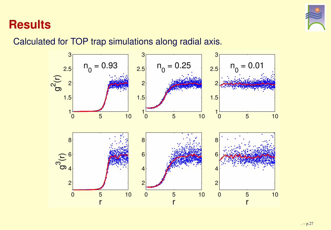
ResultsCalculated for TOP trap simulations along radial axis.

0 5 101

1.5

2

2.5

3g2 (r)

n0 = 0.93

0 5 10

2

4

6

8

g3 (r)

r

0 5 101

1.5

2

2.5

3

n0 = 0.25

0 5 10

2

4

6

8

r

0 5 101

1.5

2

2.5

3

n0 = 0.01

0 5 10

2

4

6

8

r

. – p.27

Shift of Tc with interactionstrength

. – p.28

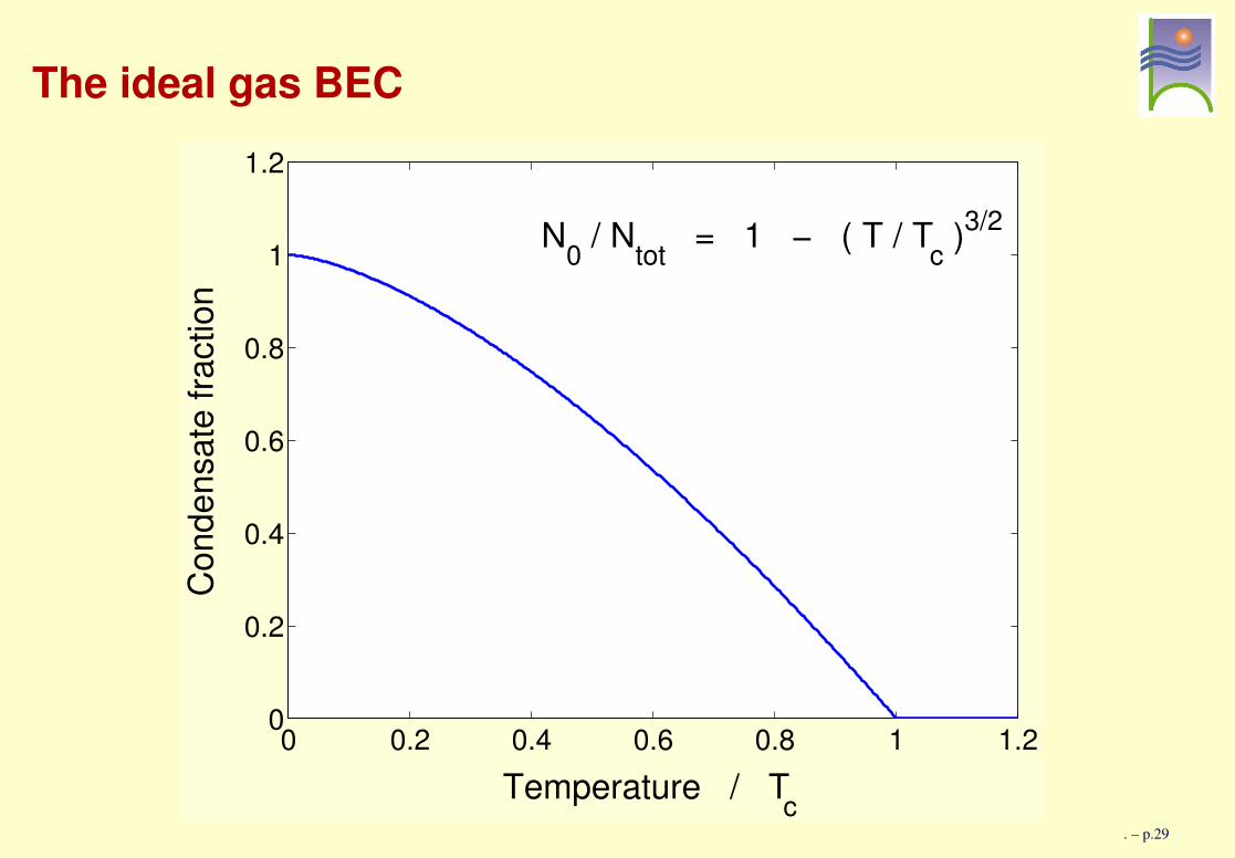
The ideal gas BEC

0 0.2 0.4 0.6 0.8 1 1.20

0.2

0.4

0.6

0.8

1

1.2

N0 / Ntot = 1 − ( T / Tc )3/2

Temperature / Tc

Cond

ensa

te fr

actio

n

. – p.29

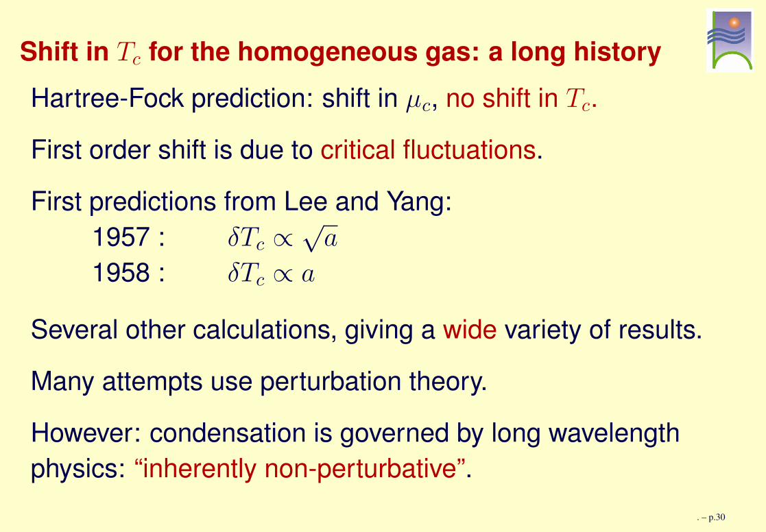
Shift in Tc for the homogeneous gas: a long historyHartree-Fock prediction: shift in µc, no shift in Tc.

First order shift is due to critical fluctuations.

First predictions from Lee and Yang:1957 : δTc ∝

√a

1958 : δTc ∝ a

Several other calculations, giving a wide variety of results.

Many attempts use perturbation theory.

However: condensation is governed by long wavelengthphysics: “inherently non-perturbative”.

. – p.30

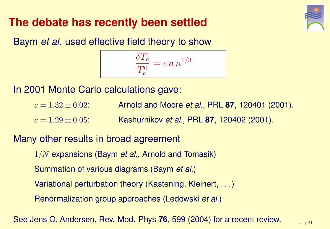
The debate has recently been settledBaym et al. used effective field theory to show

δTc

T 0c

= c a n1/3

In 2001 Monte Carlo calculations gave:c = 1.32 ± 0.02: Arnold and Moore et al., PRL 87, 120401 (2001).c = 1.29 ± 0.05: Kashurnikov et al., PRL 87, 120402 (2001).

Many other results in broad agreement1/N expansions (Baym et al., Arnold and Tomasik)Summation of various diagrams (Baym et al.)Variational perturbation theory (Kastening, Kleinert, . . . )Renormalization group approaches (Ledowski et al.)

See Jens O. Andersen, Rev. Mod. Phys 76, 599 (2004) for a recent review. . – p.31

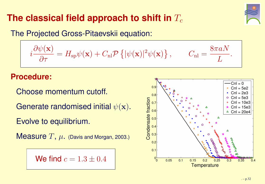
The classical field approach to shift in Tc

The Projected Gross-Pitaevskii equation:

i∂ψ(x)

∂τ= Hspψ(x) + CnlP

{

|ψ(x)|2ψ(x)}

, Cnl =8πaN

L.

Procedure:

Choose momentum cutoff.

Generate randomised initial ψ(x).

Evolve to equilibrium.

Measure T , µ. (Davis and Morgan, 2003.)

We find c = 1.3 ± 0.4 0 0.05 0.1 0.15 0.2 0.25 0.3 0.35 0.40

0.1

0.2

0.3

0.4

0.5

0.6

0.7

0.8

0.9

1

Temperature

Cond

ensa

te fr

actio

n

Cnl = 0Cnl = 5e2Cnl = 2e3Cnl = 5e3Cnl = 10e3Cnl = 15e3Cnl = 20e4

. – p.32

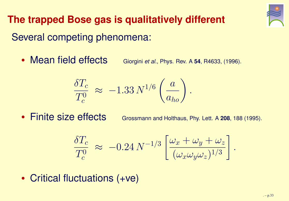
The trapped Bose gas is qualitatively differentSeveral competing phenomena:

• Mean field effects Giorgini et al., Phys. Rev. A 54, R4633, (1996).

δTcT 0c

≈ −1.33N 1/6

(

a

aho

)

.

• Finite size effects Grossmann and Holthaus, Phy. Lett. A 208, 188 (1995).

δTcT 0c

≈ −0.24N−1/3

[

ωx + ωy + ωz(ωxωyωz)1/3

]

.

• Critical fluctuations (+ve). – p.33

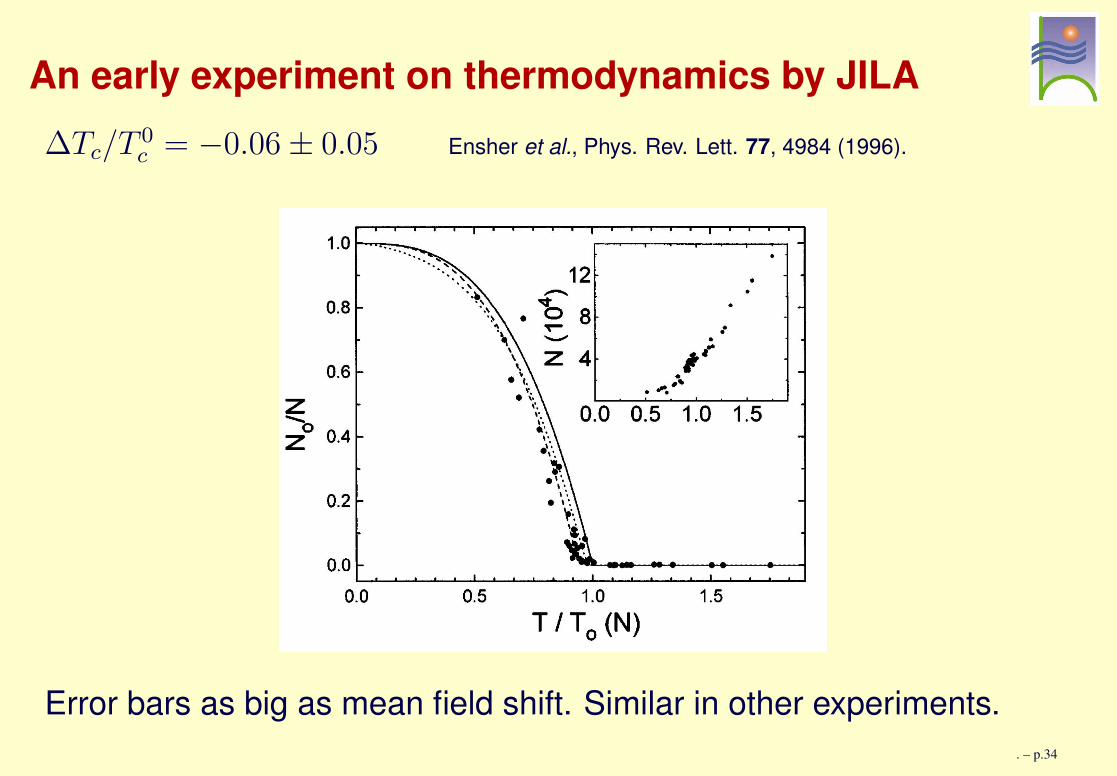
An early experiment on thermodynamics by JILA∆Tc/T

0c = −0.06 ± 0.05 Ensher et al., Phys. Rev. Lett. 77, 4984 (1996).

Error bars as big as mean field shift. Similar in other experiments.. – p.34

Other shift in Tc calculations for the trapped gasSecond order calculation using lattice result.P. Arnold and B. Tomasik, Phys. Rev. A 64, 053609 (2001).

Mean field shift for power law potentials.O. Zobay, J. Phys. B 37, 2593 (2004).

Renormalization group approach for power law potentials.O. Zobay, G. Metikas and G. Alber, Phys. Rev. A 69, 063615 (2004).

Variational perturbation theory for power law potentials.O. Zobay, G. Metikas and H. Kleinert, Phys. Rev. A 71, 043614 (2005).

All of these are in the thermodynamic limit.Also — no comparison with experiment.

. – p.35

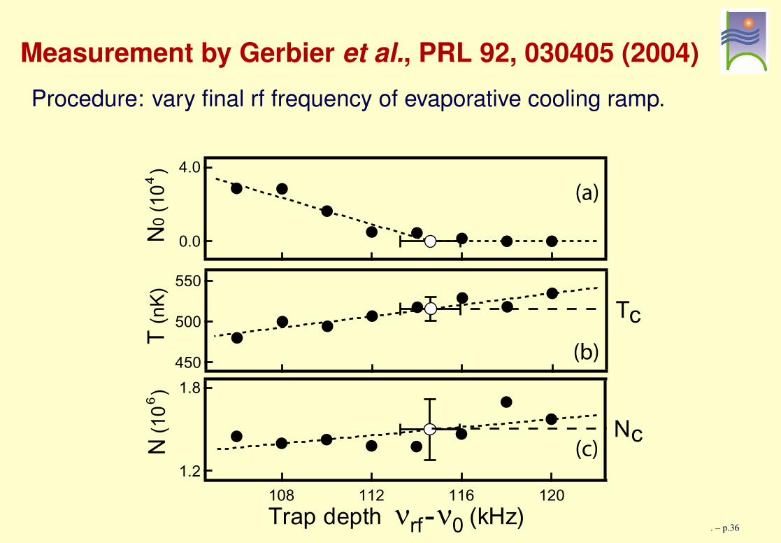
Measurement by Gerbier et al., PRL 92, 030405 (2004)Procedure: vary final rf frequency of evaporative cooling ramp.

T(n

K)

N0

(10

)4

N(1

0)

6

Trap depth νrf-ν0

(kHz)

T

N

c

c

(a)

(c)

(b)

550

500

450

1.8

1.2

120116112108

4.0

0.0

. – p.36

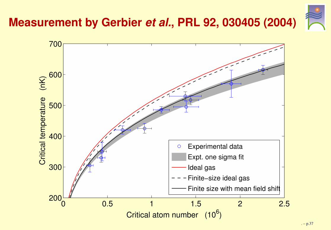
Measurement by Gerbier et al., PRL 92, 030405 (2004)

0 0.5 1 1.5 2 2.5200

300

400

500

600

700

Critical atom number (106)

Critic

al te

mpe

ratu

re

(nK)

Experimental dataExpt. one sigma fitIdeal gasFinite−size ideal gasFinite size with mean field shift

. – p.37

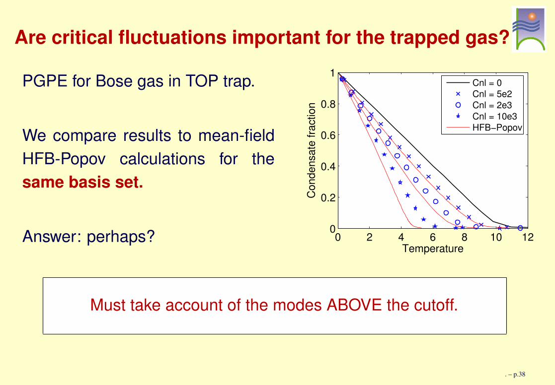
Are critical fluctuations important for the trapped gas?

PGPE for Bose gas in TOP trap.

We compare results to mean-fieldHFB-Popov calculations for thesame basis set.

Answer: perhaps? 0 2 4 6 8 10 120

0.2

0.4

0.6

0.8

1

Temperature

Cond

ensa

te fr

actio

n

Cnl = 0Cnl = 5e2Cnl = 2e3Cnl = 10e3HFB−Popov

Must take account of the modes ABOVE the cutoff.

. – p.38

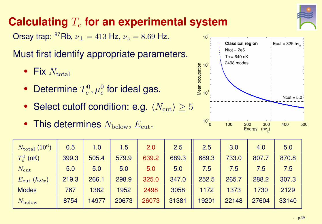
Calculating Tc for an experimental systemOrsay trap: 87Rb, ν⊥ = 413 Hz, νz = 8.69 Hz.

Must first identify appropriate parameters.• Fix Ntotal

• Determine T 0c , µ

0c for ideal gas.

• Select cutoff condition: e.g. 〈Ncut〉 ≥ 5

• This determines Nbelow, Ecut. 0 100 200 300 400 500100

101

102

103

Mea

n oc

cupa

tion

Energy (hνx)

Ecut = 325 hνx

Ncut = 5.0

Classical regionNtot = 2e6Tc = 640 nK2498 modes

Ntotal (106) 0.5 1.0 1.5 2.0 2.5 2.5 3.0 4.0 5.0T 0

c (nK) 399.3 505.4 579.9 639.2 689.3 689.3 733.0 807.7 870.8Ncut 5.0 5.0 5.0 5.0 5.0 7.5 7.5 7.5 7.5Ecut (~ωx) 219.3 266.1 298.9 325.0 347.0 252.5 265.7 288.2 307.3Modes 767 1382 1952 2498 3058 1172 1373 1730 2129Nbelow 8754 14977 20673 26073 31381 19201 22148 27604 33140

. – p.39

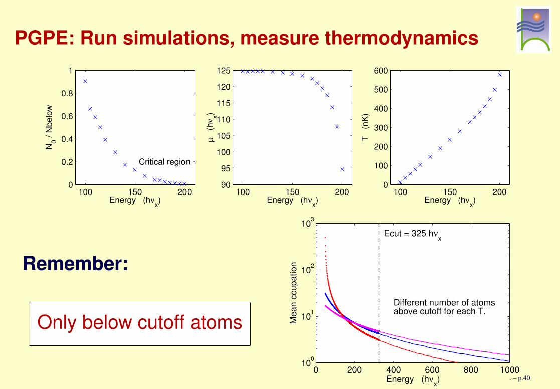
PGPE: Run simulations, measure thermodynamics

100 150 2000

0.2

0.4

0.6

0.8

1

Energy (hνx)

N 0 / Nb

elow

Critical region

100 150 20090

95

100

105

110

115

120

125

Energy (hνx)µ

(hν

x)

100 150 2000

100

200

300

400

500

600

Energy (hνx)

T (

nK)

Remember:

Only below cutoff atoms

0 200 400 600 800 1000100

101

102

103

Mea

n cc

upat

ion

Energy (hνx)

Ecut = 325 hνx

Different number of atomsabove cutoff for each T.

. – p.40

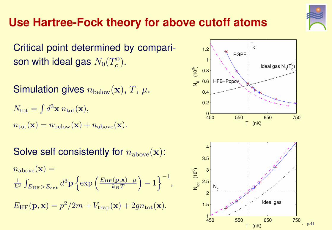
Use Hartree-Fock theory for above cutoff atoms

Critical point determined by compari-son with ideal gas N0(T

0c ).

Simulation gives nbelow(x), T , µ.

Ntot =∫

d3x ntot(x),

ntot(x) = nbelow(x) + nabove(x).

Solve self consistently for nabove(x):nabove(x) =

1h3

∫

EHF>Ecut

d3p

{

exp(

EHF(p,x)−µ

kBT

)

− 1}−1

,

EHF(p,x) = p2/2m+ Vtrap(x) + 2gntot(x).

450 550 650 7500

0.2

0.4

0.6

0.8

1

1.2

T (nK)

N 0 (1

03 )

PGPE

HFB−Popov

Tc

Ideal gas N0(Tc0)

450 550 650 7501

1.5

2

2.5

3

3.5

4

T (nK)

N tot

(106 )

Ideal gas

Nc

. – p.41

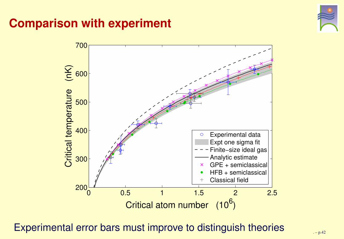
Comparison with experiment

0 0.5 1 1.5 2 2.5200

300

400

500

600

700

Critical atom number (106)

Critic

al te

mpe

ratu

re

(nK)

Experimental dataExpt one sigma fitFinite−size ideal gasAnalytic estimateGPE + semiclassicalHFB + semiclassicalClassical field

Experimental error bars must improve to distinguish theories . – p.42

Quantum simulations withclassical fields

. – p.43

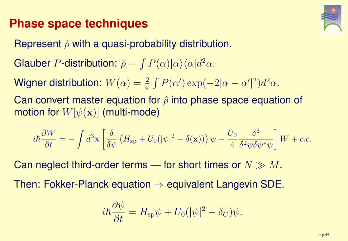
Phase space techniquesRepresent ρ with a quasi-probability distribution.

Glauber P -distribution: ρ =∫

P (α)|α〉〈α|d2α.

Wigner distribution: W (α) = 2π

∫

P (α′) exp(−2|α− α′|2)d2α.Can convert master equation for ρ into phase space equation ofmotion for W [ψ(x)] (multi-mode)

i~∂W

∂t= −

∫

d3x

[

δ

δψ

(

Hsp + U0(|ψ|2 − δ(x)))

ψ − U0

4

δ3

δ2ψδψ∗ψ

]

W + c.c.

Can neglect third-order terms — for short times or N �M .

Then: Fokker-Planck equation ⇒ equivalent Langevin SDE.

i~∂ψ

∂t= Hspψ + U0(|ψ|2 − δC)ψ.

. – p.44

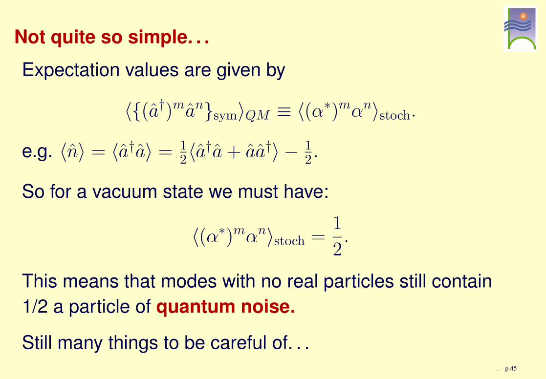
Not quite so simple. . .Expectation values are given by

〈{(a†)man}sym〉QM ≡ 〈(α∗)mαn〉stoch.

e.g. 〈n〉 = 〈a†a〉 = 12〈a†a+ aa†〉 − 1

2 .

So for a vacuum state we must have:

〈(α∗)mαn〉stoch =1

2.

This means that modes with no real particles still contain1/2 a particle of quantum noise.

Still many things to be careful of. . .. – p.45

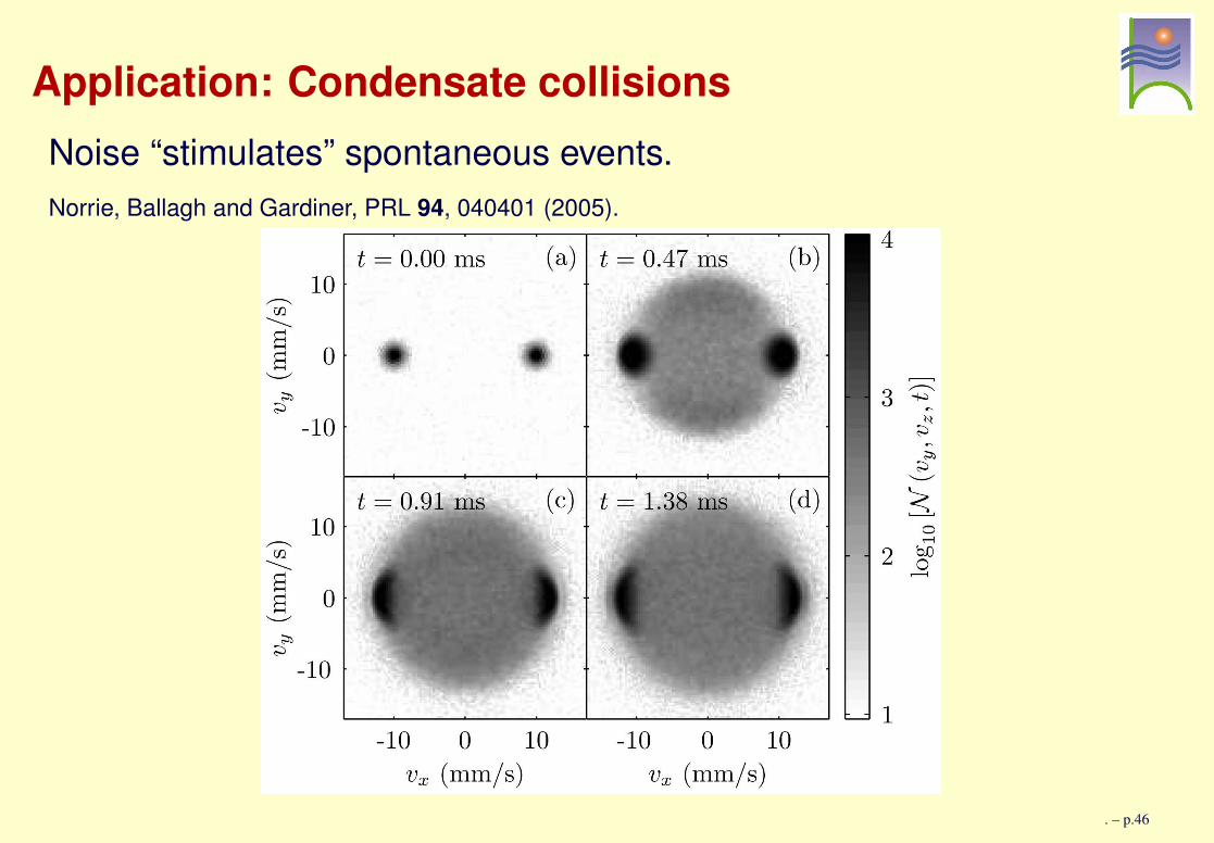
Application: Condensate collisionsNoise “stimulates” spontaneous events.Norrie, Ballagh and Gardiner, PRL 94, 040401 (2005).

. – p.46

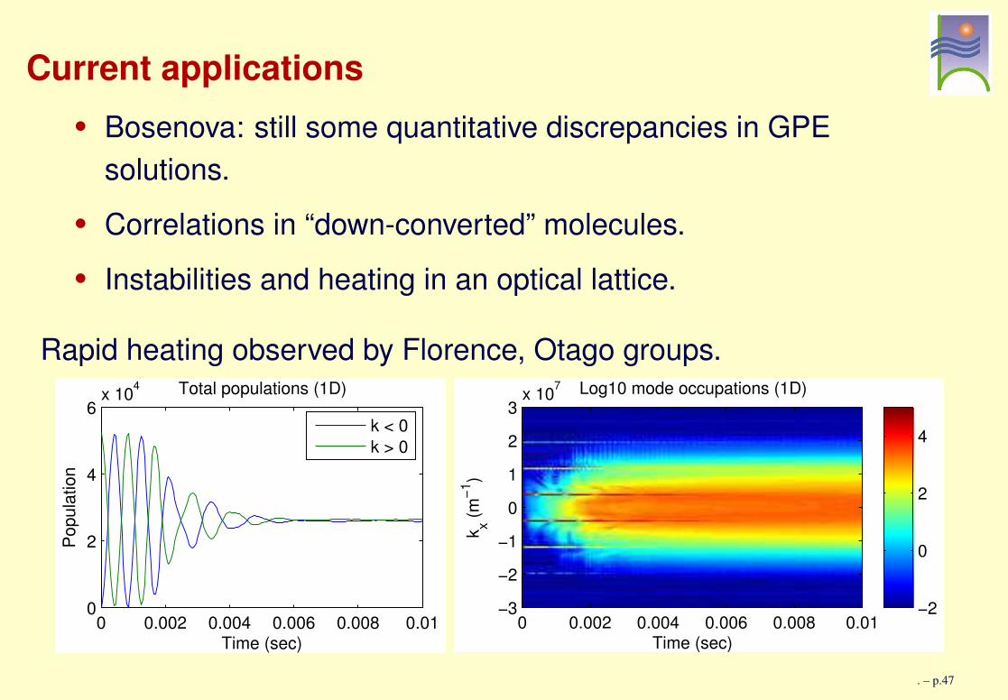
Current applications• Bosenova: still some quantitative discrepancies in GPE

solutions.• Correlations in “down-converted” molecules.• Instabilities and heating in an optical lattice.

Rapid heating observed by Florence, Otago groups.

0 0.002 0.004 0.006 0.008 0.010

2

4

6x 104

Time (sec)

Popu

latio

n

Total populations (1D)

k < 0k > 0

Time (sec)

k x (m−1

)

Log10 mode occupations (1D)

0 0.002 0.004 0.006 0.008 0.01−3

−2

−1

0

1

2

3x 107

−2

0

2

4

. – p.47

Stochastic GPE approach Gardiner and Davis, J. Phys. B 36, 4731 (2003).

• Split field operator as earlier: Ψ = ψ + η.

• Treat high-lying modes of η as a bath: µ, T .• Derive Wigner equations for classical region.

⇒ GPE with growth terms and thermal driving noise.

Similar to approach of Stoof, derived via Keldysh formalism.

Applications:• Condensate growth.• Formation of vortex lattices.

See forthcoming work from Bradley and Gardiner.

. – p.48

Summary

• Finite temperature Bose gases.• Introduction to classical fields.• Simulations of classical fields via PGPE.• Shift in Tc for interacting Bose gases.• Quantum simulations with classical fields.

Thanks to: Blair Blakie, Ashton Bradley, Chris Foster, AndyFerris, Crispin Gardiner, Sam Morgan, Keith Burnett.

. – p.49