Classical and Quantum Probabilities as Truth Values

arX

iv:1

102.

2213

v1 [

quan

t-ph

] 1

0 Fe

b 20

11

Classical and Quantum Probabilities

as Truth Values

Andreas Doring∗ and Chris J. Isham†

February, 2011

Abstract

We show how probabilities can be treated as truth values in suit-able sheaf topoi. The scheme developed in this paper is very generaland applies to both classical and quantum physics. On the quantumside, the results are a natural extension of our existing work on atopos approach to quantum theory. Earlier results on the represen-tation of arbitrary quantum states are complemented with a purelylogical perspective.

“Fate laughs at probabilities.”E.G. Bulwer-Lytton, from Eugene Aram (1832)

1 Introduction

In a long series of papers, we and our collaborators have shown how quantumtheory can be re-expressed as a type of ‘classical physics’ in the topos ofpresheaves (i.e., set-valued contravariant functors) on the partially-orderedset all commutative von Neumann sub-algebras of the algebra of all boundedoperators on the quantum-theory Hilbert space H [1, 2, 3, 4, 5, 6, 7, 8, 10].These ideas have been further developed by Caspers, Heunen, Landsman,Spitters, and Wolters in a way that emphasises the internal structure of the

∗[email protected]†[email protected]

1

topos [14, 15, 16, 17, 18, 19]. Flori has presented a topos formulation ofconsistent histories in [13].

The reformulation of quantum theory presented in these articles is a radi-cal departure from the usual Hilbert space formalism. All aspects of quantumtheory—states and state space, physical quantities, the Born rule, etc.—finda new mathematical representation, which also provides the possibility ofa novel conceptual understanding. In particular, an observer-independent,non-instrumentalist interpretation becomes possible. For this reason, we callthe new formalism ‘neo-realist’.

Of course, many open questions remain. This article deals with aspectsof probability as it shows up in both classical and quantum physics. As wewill see, in both cases the usual probabilistic description can be absorbedinto the logical framework supplied by topos theory.1

The interpretation of probability theory has been discussed endlessly afterthe Renaissance endorsed it as a respectable subject for study. In longevity,the subject shares the peristalithic nature of debates about the conceptualmeaning of quantum theory. Every physicist even mildly interested in philo-sophical questions will have heard about the range of different, incompatibleviewpoints about probability: frequentist vs. Bayesian vs. propensity; objec-tive vs. subjective probabilities; classical vs. quantum probabilities; epistemic(lack-of-knowledge) vs. irreducible probabilities; and a bewildering range ofcombinations of those.

We cannot hope to solve this debate here, but some useful remarks canemade from the viewpoint of physics. While most scientists lean naturallytowards the relative-frequency/frequentist view on probability, this interpre-tation is limited because it cannot be used to assign a probability to theoutcome of a single experiment.2 By definition, the frequentist interpreta-tion requires a large ensemble of similar systems on which an experiment isperformed, or a large number of repetitions of the experiment on a singlesystem.

A particular challenge is posed by those physical situations in which a fre-quentist interpretation cannot apply, even in principle. For example, if thewhole universe is regarded as a single entity, as in cosmology, then clearlythere are no multiple copies of the system. Moreover, the instrumentalist

1As a side remark, we do not see quantum theory fundamentally as some kind of gen-eralised probability theory. Such a viewpoint is almost invariably based on an operationalview of physics and, worse, usually comes with a very unclear ontology of both probabilitiesthemselves and the objects or processes to which they apply.

2It is always interesting to reflect on what a weather forecaster really means when heor she says ”There is 80% chance of snow tomorrow”.

2

concept of an ‘experiment’ performed on the entire universe is meaningless,since there is no external observer or agent who could perform such an experi-ment. This renders problematic both quantum cosmology and stochastic clas-sical cosmology unless probabilities can be understood in non-instrumentalistterms. This argument applies also to subsystems of the universe providedthey are sufficiently large and unique to make impossible the preparation ofan ensemble of similar systems, or repetitions of an experiment on the samesystem.

Of course, in most of science there is a valid instrumentalist view in whichthe world is divided into a system, or ensemble of systems, and an observer.The system, or ensemble, shows probabilistic behaviour when an observerperforms experiments on it. In the ensuing two-level ontology the systemand the observer have very different conceptual status. Frequentist viewsof probability typically lead to such a dualism. A Bayesian view, in whichprobabilities are primarily states of knowledge or evidence, also presupposesa divide between system and observer and is based on an operational way ofthinking about physical systems.

Such an operational view does not readily extend to quantum cosmol-ogy.3 Hence, it is desirable to have a (more) realist formulation of quantumtheory—or, potentially, more general theories—that could apply meaning-fully to the whole universe. This desire to avoid the two-level ontology of op-erational/instrumentalist approaches is one of the motivations for the toposapproach to the formulation of physical theories.

In our previous work it was shown in detail how pure quantum states andpropositions are represented in the topos formalism and how truth values canbe assigned to all propositions, without any reference to observers, measure-ments or other instrumentalist concepts. In fact, for pure quantum states,probabilities are replaced by truth values which are given by the structureof the topos itself. For the specific presheaf topoi used in our reformulationof quantum theory, a truth value is a lower set in the set V(H) (which ispartially ordered under inclusion) of commutative subalgebras of the alge-bra, B(H), of all bounded operators on H. We only consider non-trivial,commutative von Neumann subalgebras V ⊂ B(H) that contain the identityoperator. Each V ∈ V(H) can be seen as providing a classical perspective onthe quantum system, with smaller commutative subalgebras giving a more‘coarse-grained’ perspective than bigger ones.

A truth-value is therefore a collection of classical perspectives from which

3We are aware of many-worlds approaches and the attempts to (re)define probabilitiesin such a formalism. However, we are not very enthusiastic about these schemes.

3

a given proposition is true. The fact that a truth value is a lower set in V(H)expresses the idea that once a proposition is ‘true from the classical perspec-tive V ’, upon coarse-graining to smaller subalgebras V ′ ⊂ V , the propositionshould stay true. The elements4 V ∈ V(H) are also called contexts or, bymathematicians, stages of truth. It is easy to see that there are uncountablymany possible truth values if dim(H) > 1 (compare this with the uncountablymany probabilities in the interval [0, 1].)

The treatment of pure states in the topos approach makes it unnecessaryto speak of probabilities in any fundamental way. However, at first sightmixed states cannot be treated similarly. Since we aim at a formalism thatcan be interpreted in a (neo-)realist way, it seems most appropriate to regardprobabilities as objective. More specifically, we lean towards an interpreta-tion of probabilities as propensities. Since the probabilities associated withpure quantum states are absorbed into the logical structure given by thetopos, we aspire to find a ‘logical reformulation’ for the probabilities associ-ated with mixed states as well. As we will see, this necessitates an extensionof the topos used so far for quantum theory. Probabilities are thereby builtinto the mathematical structures in an intrinsic manner. They are tied upwith the internal logic of the topos and do not show up as external entitiesto be introduced when speaking about experiments.

We finally remark that all constructions shown here work for arbitrary vonNeumann algebras5 and arbitrary states, normal or non-normal. The moregeneral proofs need no extra effort, though interpretational subtleties relatingto non-normal states may arise. For simplicity and clarity of presentation,we use here only B(H) as the algebra of physical quantities of a quantumsystem and pure or mixed (i.e., normal) states.

2 The Topos Approach and Mixed States

2.1 Some basic definitions

There are several articles giving an introduction to the topos approach toquantum theory [9, 10, 12] and only a few ingredients are sketched here. Weassume some familiarity with basic aspects of category and topos theory and

4Strictly speaking, V(H) is a category whose objects are the commutative sub-algebrasV . It is therefore more accurate to write V ∈ Ob(V(H)), rather than V ∈ V(H), and thiswe did in our earlier papers. However, here, for the sake of simplicity, we use the latternotation.

5For some results, the algebra must not have a type I2-summand.

4

of functional analysis.

A key feature of the topos approach is the existence for each quantumsystem of an object that is functionally analogous to the state space of aclassical system. This ‘quantum state space’, Σ, is a presheaf (i.e., a set-valued, contravariant functor) on the poset V(H) of abelian subalgebras ofB(H), the algebra of physical quantities (or observables) of the quantumsystem. The collection of all such functors is a topos, denoted SetsV(H)op .The poset V(H) and object Σ are known respectively as the context categoryand spectral presheaf.

Definition 2.1 The spectral presheaf, Σ, is defined over the context cate-gory, V(H), as follows:

(i) On objects V ∈ V(H), ΣV is the Gel’fand spectrum of the commutativevon Neumann algebra V .

(ii) On morphisms iV ′V : V ′ → V ( i.e., V ′ ⊆ V ), the presheaf functionsΣ(iV ′V ) : ΣV → ΣV ′ are defined as

Σ(iV ′V )(λ) := λ|V ′ (2.1)

for λ ∈ ΣV . Here λ|V ′ denotes the restriction to V ′ of the spectralelement λ ∈ ΣV .

A sub-object (i.e., sub-presheaf) S is said to be clopen if SV is a clopenset in ΣV for all V ∈ V(H). The clopen sub-objects of Σ form a completeHeyting algebra (Theorem 2.5 in [6]), denoted Subcl(Σ).

Propositions in physics are usually of the form “Aε∆”, which in classicalphysics would read “the physical quantity A has a value, and that value lies inthe (Borel) set ∆ ⊆ R of real numbers”. Using the spectral theorem for self-adjoint operators, a proposition “Aε∆” is represented in quantum theoryby the spectral projector E[Aε∆]. It was shown in [6] that there is a mapδ : P(H) → Subcl(Σ), called ‘daseinisation of projection operators’, whichsends each projection operator P to a clopen sub-object δ(P ). In this way,

a proposition “Aε∆” is represented by the clopen sub-object δ(E[Aε∆]) ofΣ. This is analogous to classical physics where propositions are representedby (measurable) subsets of the classical state space.

The sub-object δ(P ) is constructed in a two-step process. First, onedefines, for all V ∈ V(H),

δ(P )V :=∧

Q ∈ P(V ) | Q P, (2.2)

5

which gives the ‘best’ approximation to P from above by a projector in thelattice, P(V ), of projection operators in the context V . The associationV 7→ δ(P )V is a global element, denoted δ(P ), of the outer presheaf O [1, 3]:

Definition 2.2 The outer presheaf, O, is defined as follows :

(i) On objects V ∈ V(H), OV := P(V ).

(ii) On morphisms iV ′V : V ′ ⊆ V , the mapping O(iV ′V ) : OV → OV ′ isO(iV ′V )(P ) := δ(P )V ′ for all P ∈ P(V ).

The second step uses the existence of a monic arrow, ι : O → PclΣ, fromO to the clopen power object, PclΣ, of Σ [6]. This sub-object, PclΣ, of thepower object PΣ has the property that its global elements are clopen sub-objects of Σ, whereas the global elements of PΣ are arbitrary sub-objects[6]. The construction of ι exploits the fact that for any commutative vonNeumann algebra V , there is an isomorphism of complete Boolean algebras

αV : P(V ) = OV → Cl(ΣV ), (2.3)

P 7→ λ ∈ ΣV | λ(P ) = 1

between the projections in V and the clopen subsets of the Gel’fand spectrum,ΣV , of V . Given a projection P ∈ P(V ), we define

SP := αV (P ), (2.4)

and given a clopen subset S ⊆ ΣV , we define

PS := α−1V (S). (2.5)

Thus locally, i.e., in each context V , we can switch between clopen subsetsand projections.

Applying this to the family δ(P )V , V ∈ V(H), of projectors, gives afamily Sδ(P )V

⊆ ΣV , V ∈ V(H), of clopen subsets. This family of clopen

subsets forms a clopen sub-object, denoted δ(P ), of Σ. Equivalently, the

global element δ(P ) : 1 → O defined by (2.2) gives rise via ι : O → PclΣ toa global element 1 → O → PclΣ of PclΣ, and hence to the clopen sub-objectδ(P ).

Given a (normalised) vector state |ψ〉, we now form

w|ψ〉 := δ( |ψ〉〈ψ| ) ∈ Subcl(Σ). (2.6)

6

This clopen sub-object is the topos representative of the pure state |ψ〉: wecall w |ψ〉 the pseudo-state associated with |ψ〉.

To each vector state |ψ〉 ∈ H and physical proposition “Aε∆” therecorresponds the ‘topos truth value’ ν

(

Aε∆; |ψ〉)

∈ ΓΩ defined at each stageV ∈ V(H) as,

ν(

Aε∆; |ψ〉)

(V ) := V ′ ⊆ V | 〈ψ| δ(E[Aε∆])V ′ |ψ〉 = 1. (2.7)

We also write

ν(

P ; |ψ〉)

(V ) := V ′ ⊆ V | 〈ψ| δ(P )V ′ |ψ〉 = 1 (2.8)

for any projection operator P on H.

This truth value, which is a sieve on V , can be understood as the ‘degree’to which the sub-object w |ψ〉 that represents the pure state is contained in thesub-object δ(E[Aε∆]) that represents the proposition. This degree is simply

the collection of all those contexts V ∈ V(H) such that w|ψ〉V ⊆ δ(E[Aε∆])

V.

2.2 The problem of mixed states

A very interesting (and important) question is how mixed states should betreated in this topos formalism. In its basic form, a mixed state is just a col-lection of vectors and ‘weights’, |ψ1〉, |ψ2〉, . . . , |ψN〉; r1, r2, . . . , rN, where∑N

i=1 ri = 1 (we allow N = ∞). In standard quantum theory, the assump-tion that the quantum probabilities are stochastically independent from the‘weights’ r1, r2, . . . , rN , leads via elementary probability arguments to thefamiliar definition of the associated density matrix as ρ :=

∑Ni=1 ri |ψi〉〈ψi|

and hence to the familiar expressions in which, for example, tr(ρA) replaces〈ψ| A |ψ〉.

The important challenge is to find an analogue for ρ of the truth value in(2.7) for vector states |ψ〉, and in such a way that density matrices areseparated by this expression. Of course, the vector |ψ〉 in (2.7) can bereplaced with ρ to give the sieve on V

ν(

Aε∆; ρ)

(V ) := V ′ ⊆ V | tr(

ρ δ(E[Aε∆])V ′

)

= 1, (2.9)

but this is not adequate for our needs as it does not separate density matrices.

For example, let H be a three-dimensional Hilbert space with a chosenbasis, and let ρ = diag(1

2, 12, 0) and ρ = diag(3

4, 14, 0) be two density matrices

that are diagonal with respect to this basis. Then tr(ρP ) = 1 if and only

7

if tr(ρP ) = 1 if and only if P P1 + P2, where P1, P2 are the projectionsonto the rays determined by the first two basis vectors. In other words, ρand ρ have the same support, namely P1 + P2, and the topos truth valueν(

Aε∆; ρ)

∈ ΓΩ (given by the family ν(

Aε∆; ρ)

(V ), V ∈ V(H), of sievesdefined above) depends only on the supports, not on the actual weights, inρ and ρ.

As pointed out in [3], there exists a one-parameter family of valuationsdefined for all V ∈ V(H) as

ν(

Aε∆; ρ)r(V ) := V ′ ⊆ V | tr

(

ρ δ(E[Aε∆])V ′

)

≥ r (2.10)

where r ∈ (0, 1]. (One could allow r = 0, but clearly, the condition thenis trivially fulfilled and the valuation ν(−;−)0 gives the truth value ‘totallytrue’, represented by the maximal sieve at each stage, for all states ρ andall propositions “Aε∆”.) The authors of [3] could find no use for these r-modified ‘truth’ values. However, it transpires that this family of valuationsdoes separate density matrices, which is very suggestive of how to proceed.

Indeed, the main result of this paper is to show how the one-parameterfamily in (2.10) can be regarded as a single valuation in a particular extensionof the topos SetsV(H)op . By this means we will achieve a completely topos-internal description of arbitrary (normal) quantum states ρ.

At this point we remark that there is another topos perspective on densitymatrices that at first sight appears to be very different from the one above.One of us (AD) has shown how each density matrix, ρ, gives rise to a ‘prob-ability’ (pre-)measure, µρ, on Subcl(Σ) [11]. This function µρ : Subcl(Σ) →Γ[0, 1] is defined at all stages V ∈ V(H) by

µρ(S)(V ) := tr(ρ PSV ) (2.11)

where PSV is the projection operator in P(V ) that corresponds to the com-

ponent SV of the clopen sub-object S at stage V . Here, [0, 1] denotes thepresheaf of [0, 1]-valued, nowhere-increasing functions on the poset/categoryV(H). It can readily be checked that this family of measures separates den-sity matrices.

Conversely, [0, 1]-valued probability measures on the spectral presheafΣ can be defined abstractly, with the clopen sub-objects playing the role ofmeasurable subsets. Provided the Hilbert space H has at least dimensionthree, from each such measure, µ, one can construct a unique quantum stateρµ : B(H) → C, such that µρ

µ

= µ.6 The existence of such measures is

6For the more general case of von Neumann algebras treated in [11], the condition isthat the von Neumann algebra has no summand of type I2.

8

in accord with our general slogan that “Quantum physics is equivalent toclassical physics in the topos SetsV(H)op”.

The construction in (2.11) can be applied to a (normalised) vector state|ψ〉, to give

µ |ψ〉〈ψ| (S)(V ) := 〈ψ| PSV |ψ〉 (2.12)

at all stages V . In particular, for the sub-object SAε∆ of Σ associated withthe spectral projector E(Aε∆) we get

µ |ψ〉〈ψ| (SAε∆)(V ) = 〈ψ| δ(E[Aε∆])V |ψ〉 (2.13)

Thus, for each state |ψ〉, a proposition “Aε∆” is associated with two,quite different, mathematical entities:

(i) the Heyting-algebra valued topos truth value ν(

Aε∆; |ψ〉)

∈ ΓΩ de-fined in (2.7) as

ν(

Aε∆; |ψ〉)

(V ) := V ′ ⊆ V | 〈ψ| δ(E[Aε∆])V ′ |ψ〉 = 1 (2.14)

for all V ∈ V(H); and

(ii) the [0, 1]-valued measure µ |ψ〉〈ψ| on Subcl(Σ) defined in (2.13) as

µ |ψ〉〈ψ| (SAε∆)(V ) := 〈ψ| δ(E[Aε∆])V |ψ〉 (2.15)

for all V ∈ V(H).

The purpose of the present paper is to study the relation between thesetwo entities, and thereby to see if there is a topos-logic representation of thegeneral, density-matrix measure, µρ in (2.11). Thus the challenge is to relatethe probability measure µρ : Subcl(Σ) → Γ[0, 1] to a topos truth value andhence to relate probability to intuitionistic logic. It is clear that the definitionin (2.9) is not adequate as, unlike the measures µρ, it fails to separate densitymatrices.

As we shall see, the one-parameter family of valuations r 7→ ν(

Aε∆; ρ)r

∈ΓΩ defined in (2.10) plays a key role. However, the incorporation of this fam-ily into a topos framework requires an extension of the original quantum toposSetsV(H)op . We will motivate this by first considering a topos perspective onclassical probability theory.

We conclude this section with a technical remark. Namely, instead oftalking about presheaves over the context category V(H), which is a poset,we can equivalently talk about sheaves if V(H) is equipped with the (lower)

9

Alexandroff topology in which the open sets are the lower sets in V(H). Then,by a standard result7 we have

Sh(V(H)A) ≃ SetsV(H)op , (2.16)

where V(H)A denotes the poset V(H) equipped with the lower Alexandrofftopology. In what follows we will move freely between the language ofpresheaves and that of sheaves—which of the two is being used should beclear from the context.

3 A Topos Representation for Probabilities

The usual description of probabilities is by numbers in the interval [0, 1],equipped with the total order inherited from R. In order to absorb prob-abilities into the logic of a topos, our goal now is to find a topos, τ , suchthat

[0, 1] ≃ ΓΩτ (3.1)

where Ωτ is the truth object in τ . A natural way of doing this is to lookfor a topological space, X , whose open sets correspond bijectively with thenumbers between 0 and 1.

Since the global elements of the sub-object classifier Ωτ are the truthvalues available in the topos τ , equation (3.1) means that probabilities willcorrespond bijectively with truth values in the topos.

A straightforward idea is to use suitable lower sets in the unit interval[0, 1]. These lower sets are required to form a topology, so the collectionof lower sets must be closed under arbitrary unions and finite intersections.The intervals of the form (0, r), where 0 ≤ r ≤ 1, form a topology. Here(0, 0) = ∅. The maximal element is (0, 1), so our topological space X actuallyis the interval (0, 1) (and not [0, 1]). When regarding (0, 1) as a topologicalspace with the topology given by the sets of the form (0, r), 0 ≤ r ≤ 1, wedenote it as (0, 1)L. We define a bijection

β : [0, 1] → O((0, 1)L) (3.2)

r 7→ (0, r).

Note also that intervals of the form (0, r] would not work: they are not closedunder arbitrary unions. Take for example all intervals (0, ri] such that ri < r0for some fixed r0 ∈ [0, 1]. Then

⋃

i(0, ri] = (0, r0).

7If A denotes the sheaf associated with the presheaf A, then, on the open set ↓V , wehave A(↓V ) = AV for all V ∈ V(H). On an arbitrary lower set L ⊆ V(H), A(L) is the(possibly empty) set of local sections of Σ over L.

10

It may seem odd that a probability r ∈ [0, 1] is represented by the (open)set (0, r), which does not contain r, but this is not problematic. In thefollowing, we will not interpret (0, r) as the collection of all probabilitiesbetween 0 and r, but as an open set, which corresponds to a truth valuein a sheaf topos. This truth value, given by the structure of the topos,corresponds to the probability r.

Now, a key idea in topos theory is that any topological space, X , should bereplaced with the topos, Sh(X), of sheaves over X . Furthermore, a standardresult is that there is an isomorphism of Heyting algebras.

O(X) ≃ ΓΩSh(X) (3.3)

It becomes clear that the topos we are seeking is Sh((0, 1)L). We will simplifythe notation ΩSh((0,1)L) to just Ω(0,1); thus

O((0, 1)L) ≃ ΓΩ(0,1). (3.4)

We denote the isomorphism as σ : O((0, 1)L) → ΓΩ(0,1). Its concrete formwill be discussed below.

It is clear that, for all stages (0, r) ∈ O((0, 1)L), the component Ω(0,1)r of

the sheaf Ω(0,1) is given by

Ω(0,1)(0,r) = (0, r′) | 0 < r′ ≤ r ∪ ∅

= (0, r′) | 0 ≤ r′ ≤ r. (3.5)

We remark that instead of describing stages as (0, r) ∈ O((0, 1)L), we canalso think of r ∈ [0, 1] by the isomorphism (3.2).

We now define a key map ℓ that takes a probability p ∈ [0, 1] into a globalsection of Ω(0,1), that is, a truth value in the topos. Roughly speaking, theidea is that p is mapped to the open set (0, p), which is a truth value inthe sheaf topos. In fact, the map ℓ that we will define is nothing but thecomposition σ β of the set isomorphisms β in (3.2) and σ in (3.4).

Concretely, we define for all p ∈ [0, 1] and all stages (0, r) ∈ O((0, 1)L)the following sieve on (0, r):

ℓ(p)(0,r) := (0, r′) ∈ O((0, 1)L) | p ≥ r′ (3.6)

= (0, r′) | r′ = minp, r (3.7)

where, by definition, (0, 0) = ∅. Thus we have

ℓ(p)(0,r) =

(0, r′) ∈ O((0, 1)L) | r′ ≤ r = Ω

(0,1)(0,r) if p ≥ r

(0, r′) ∈ O((0, 1)L) | r′ ≤ p if 0 < p < r

∅ if p = 0

(3.8)

11

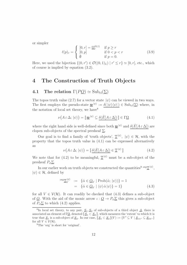
or simpler

ℓ(p)r =

[0, r] = Ω(0,1)r if p ≥ r

[0, p] if 0 < p < r

∅ if p = 0.(3.9)

Here, we used the bijection (0, r′) ∈ O((0, 1)L) | r′ ≤ r ≃ [0, r], etc., which

of course is implied by equation (3.2).

4 The Construction of Truth Objects

4.1 The relation Γ(PO) ≃ Subcl(Σ)

The topos truth value (2.7) for a vector state |ψ〉 can be viewed in two ways.The first employs the pseudo-state w

|ψ〉 := δ( |ψ〉〈ψ| ) ∈ Subcl(Σ) where, in

the notation of local set theory, we have8

ν(

Aε∆; |ψ〉)

= [[w |ψ〉 ⊆ δ(E[Aε∆]) ]] ∈ ΓΩ (4.1)

where the right hand side is well-defined since both w|ψ〉 and δ(E[Aε∆]) are

clopen sub-objects of the spectral presheaf Σ.

Our goal is to find a family of ‘truth objects’, T |ψ〉, |ψ〉 ∈ H, with theproperty that the topos truth value in (4.1) can be expressed alternativelyas

ν(

Aε∆; |ψ〉)

= [[ δ(E[Aε∆]) ∈ T |ψ〉 ]] (4.2)

We note that for (4.2) to be meaningful, T |ψ〉 must be a sub-object of thepresheaf PclΣ.

In our earlier work on truth objects we constructed the quantities9 orgT |ψ〉,|ψ〉 ∈ H, defined by

orgT|ψ〉V := α ∈ OV | Prob(α; |ψ〉) = 1

= α ∈ OV | 〈ψ| α |ψ〉 = 1 (4.3)

for all V ∈ V(H). It can readily be checked that (4.3) defines a sub-objectof O. With the aid of the monic arrow ι : O → PclΣ this gives a sub-objectof PclΣ to which (4.2) applies.

8In local set theory, to any pair, S1, S2 of sub-objects of a third object A, there isassociated an element of ΓΩ, denoted [[S1 ⊂ S2 ]], which measures the ‘extent’ to which it istrue that S1 is a sub-object of S2. In our case, [[S1 ⊂ S2 ]](V ) := V ′ ⊆ V | S1V ′ ⊆ S2V ′for all V ∈ V(H).

9The ‘org’ is short for ‘original’.

12

For discussing daseinised sub-objects of Σ like δ(E[Aε∆]) the simpledefinition in (4.3) is sufficient. However, the situation changes if we want toconsider more general sub-objects of Σ. Specifically, we want to define T |ψ〉

in such a way that[[S ∈ T |ψ〉 ]] ∈ ΓΩ (4.4)

is well-defined for any clopen sub-object, S, of Σ. This is necessary to fulfilour desire to relate topos truth values with measures on Subcl(Σ). Clopensub-objects of the form δ(E[Aε∆]) have very special properties whereas ourmeasures are defined on arbitrary clopen sub-objects of Σ. This necessitatesa new definition of the truth objects T |ψ〉, |ψ〉 ∈ H.

Evidently, clopen sub-objects of the spectral presheaf Σ are of particularinterest as the analogues of measurable subsets of a classical state space S.More precisely, as in (2.11), each quantum state ρ determines a (Γ[0, 1]-valued) ‘probability measure’, µρ, on Σ, with the clopen sub-objects play-ing the role of measurable subsets; conversely, each probability measure onSubcl(Σ) determines a unique quantum state. The proof relies on Gleason’stheorem which shows that a quantum state is determined by the values ittakes on projections. As we shall see, clopen sub-objects have componentswhich correspond to projections, hence Gleason’s theorem is applicable.

It is very desirable to be able to express all clopen sub-objects of Σ interms of projection operators as these are the mathematical entities thathave the most direct physical meaning in quantum physics and they are alsorelatively easy to manipulate.

As mentioned earlier, there is a monic arrow ι : O → PclΣ and, therefore,any global element of O leads to a clopen sub-object of Σ. However, ι isnot surjective and hence not all clopen sub-objects can be obtained in thisway. The remaining sub-objects can be recovered using the, so-called, hyper-elements of O that were introduced in [6]. This is an intermediate steptowards realising our main goal, which is to find some object X in the toposthat (i) can be defined purely in terms of projection operators; and (ii) issuch that10

ΓX ≃ Subcl(Σ) (4.5)

We start by recalling that a global element of O is a family of elementsγV ∈ OV ≃ P(V ), V ∈ V(H), such that, for all pairs iV ′V : V ′ ⊆ V we have

O(iV ′ V )(γV ) = γV ′ (4.6)

10The power object PΣ is not the correct choice as Γ(PΣ) ≃ Sub(Σ) and the latterincludes sub-objects of Σ that are not clopen; i.e., Subcl(Σ) ⊂ Sub(Σ).

13

In other wordsδ(γV )V ′ = γV ′. (4.7)

A hyper-element of O is a generalisation of this concept. Specifically, ahyper-element is a family of elements γV ∈ OV , V ∈ V(H), such that, for allpairs iV ′V : V ′ ⊆ V we have [6]

O(iV ′ V )(γV ) γV ′ (4.8)

In other wordsδ(γV )V ′ γV ′ . (4.9)

We denote the set of all hyper-elements of O as Hyp(O).

The importance of hyper-elements comes from the following results whichare proved in the Appendix.

1. There is a bijection

k : Hyp(O) → Subcl(Σ) (4.10)

k(γ)V := αV (γV ) = SγV

for all γ ∈ Hyp(O), V ∈ V(H) (see Proposition 7.1).

The inverse is

j : Subcl(Σ) → Hyp(O) (4.11)

j(S)V := α−1V (SV ) = PSV

for all S ∈ Subcl(Σ), V ∈ V(H).

2. There is a bijection

c : Sub(O) → Hyp(O) (4.12)

c(A)V :=∨

α | α ∈ AV

for A ∈ Sub(O), V ∈ V(H) (see Proposition 7.2).

The inverse is

d : Hyp(O) → Sub(O) (4.13)

d(γ)V := α ∈ OV | α γV

for all γ ∈ Hyp(O), V ∈ V(H).

14

It follows from the above that there is a bijection

f : Sub(O) → Subcl(Σ) (4.14)

f(A)V := S∨α∈AV

for all A ∈ Sub(O), V ∈ V(H). The inverse is

g : Subcl(Σ) → Sub(O) (4.15)

g(S)V := α ∈ OV | α PSV (4.16)

for all S ∈ Subcl(Σ), V ∈ V(H). We simply define f := k c and g := d jwhere the bijections c : Sub(O) → Hyp(O), k : Hyp(O) → Subcl(Σ), j :Subcl(Σ) → Hyp(O), and d : Hyp(O) → Sub(O) are defined in (4.12), (4.10),(4.11), and (4.13) respectively.

The problem posed in (4.5) can now be solved:

Proposition 4.1 The global elements of the power-object presheaf PO cor-respond bijectively with the clopen sub-objects of Σ.

Proof. We have shown above that there is a bijective correspondence

Sub(O) ≃ Subcl(Σ) (4.17)

Now for any object A a fundamental property of the power object, PA, isthat Γ(PA) ≃ Sub(A). It follows from (4.14) that

Γ(PO) ≃ Subcl(Σ) (4.18)

At this point it is worth stating the well-known specific form of a powerobject in a topos of presheaves. Specifically:

Definition 4.1 The power object PA of any presheaf A over V(H) is thepresheaf given by

(i) On objects V ∈ V(H), for all V ∈ V(H), PAV is defined as

PAV := nV : A|↓V → Ω|↓V | nV is a natural transformation (4.19)

where A|↓V

is the restriction of the presheaf A to the smaller poset ↓

V ⊂ V(H), and analogously for Ω|↓V .

15

(b) On morphisms iV ′V : V ′ → V ( i.e., V ′ ⊆ V ), the presheaf functionsPA(iV ′V ) : PAV → PAV ′ are defined as

PA(iV ′V ) : PAV → PAV ′

nV 7→ nV′|↓V (4.20)

Here, nV′|↓V is the obvious restriction of the natural transformation nV

to a natural transformation A|↓V ′ → Ω|↓V ′.

We now prove the ‘internal’ analogue of the ‘external’ isomorphism Sub(O) ≃Subcl(Σ) in (4.14), namely:

Theorem 4.2 In the presheaf topos SetsV(H)op , there is an isomorphism

PO ≃ PclΣ (4.21)

between the power objects PO and PclΣ.

Proof.

It follows from (4.19) that an equivalent definition of PA is

PAV := Sub(A|↓V ) (4.22)

for all V ∈ V(H). In this form, the presheaf maps in (4.20) are just therestriction of an object in Sub(A|↓V ) to ↓V ′ for all V ′ ⊆ V .

In particular, the Definition 4.1 (and equation (4.22)) applies to the powerobject, PO, of the outer presheaf O. The presheaf PclΣ is defined in the sameway except only clopen sub-objects of Σ are used. Thus, for all V ∈ V(H),we have

POV = Sub(O|↓V ) (4.23)

andPclΣV = Subcl(Σ|↓V ) (4.24)

However, the bijection f : Sub(O) → Subcl(Σ) in (4.14) clearly gives rise toa series of ‘local’ bijections

fV : Sub(O|↓V ) → Subcl(Σ|↓V ) (4.25)

for all V ∈ V(H). The inverse is

gV : Subcl(Σ|↓V ) → Sub(O|↓V ) (4.26)

16

These local maps are consistent with subspace inclusions iV ′V : V ′ ⊆ V ,i.e., they are the components of two (mutually inverse) natural transforma-tions

f : PO → PclΣ; g : PclΣ → PO. (4.27)

Therefore, PO can be identified with the clopen power object PclΣ.

We note that we we also have the bijections

cV : Sub(O|↓V ) → Hyp(O|↓V ) (4.28)

with inversedV : Hyp(O|↓V ) → Sub(O|↓V ). (4.29)

4.2 Generalised truth objects

We first recall from (2.8) that the topos truth value in ΓΩ for a propositionrepresented by a projection operator P is

ν(

P ; |ψ〉)

(V ) := V ′ ⊆ V | 〈ψ| δ(P )V ′ |ψ〉 = 1 (4.30)

for all V ∈ V(H). The expression in (4.30) can be usefully rewritten as

ν(

P ; |ψ〉)

(V ) := V ′ ⊆ V | δ(P )V ′ |ψ〉〈ψ| (4.31)

and, similarly, the ‘original’ truth object given in (4.3) can be rewritten asas

orgT|ψ〉V = α ∈ OV | α |ψ〉〈ψ| (4.32)

As defined in (4.32), orgT |ψ〉 is a sub-object of O. The mathematicalexpression [[ δ(P ) ∈ orgT |ψ〉 ]] only has meaning if orgT |ψ〉 can be regarded asub-object of PclΣ, which it can by virtue of the monic arrow O → PclΣ.However, in order to give meaning to the valuations [[S ∈ T |ψ〉 ]] for anarbitrary clopen sub-object, S of Σ we need to find a new expression for atruth object that does not ‘factor’ through the monic O → PclΣ.

Using the isomorphism PO ≃ PclΣ proved in Proposition 4.2, the newtruth object can be regarded as a sub-object of PO. The concrete form ofPO can be written in several equivalent ways using the local isomorphisms

POV = Sub(O|↓V ) ≃ Hyp(O|↓V ) ≃ Subcl(Σ|↓V ). (4.33)

Specifically, we define the new truth object T |ψ〉 ⊂ PO as

T|ψ〉V := A ∈ Sub(O|↓V ) | ∀V

′ ⊆ V, |ψ〉〈ψ| ∈ AV ′ (4.34)

≃ γ ∈ Hyp(O|↓V ) | ∀V′ ⊆ V, |ψ〉〈ψ| γV ′ (4.35)

≃ S ∈ Subcl(Σ|↓V ) | ∀V′ ⊆ V, |ψ〉〈ψ| PSV ′ (4.36)

17

for all V ∈ V(H). For inclusions iV ′V : V ′ ⊆ V , the presheaf maps T |ψ〉(iV ′V ) :

T|ψ〉V → T

|ψ〉V ′ are just the obvious restrictions from ↓V to ↓V ′.

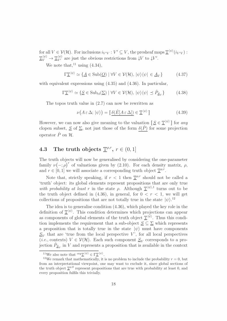
We note that,11 using (4.34),

ΓT |ψ〉 ≃ A ∈ Sub(O) | ∀V ∈ V(H), |ψ〉〈ψ| ∈ AV (4.37)

with equivalent expressions using (4.35) and (4.36). In particular,

ΓT |ψ〉 ≃ S ∈ Subcl(Σ) | ∀V ∈ V(H), |ψ〉〈ψ| PSV (4.38)

The topos truth value in (2.7) can now be rewritten as

ν(

Aε∆; |ψ〉)

= [[ δ(E[Aε∆]) ∈ T |ψ〉 ]] (4.39)

However, we can now also give meaning to the valuation [[S ∈ T |ψ〉 ]] for anyclopen subset, S of Σ, not just those of the form δ(P ) for some projection

operator P on H.

4.3 The truth objects Tρ,r, r ∈ (0, 1]

The truth objects will now be generalised by considering the one-parameterfamily ν

(

−; ρ)r

of valuations given by (2.10). For each density matrix, ρ,and r ∈ [0, 1] we will associate a corresponding truth object Tρ,r.

Note that, strictly speaking, if r < 1 then Tρ,r should not be called a‘truth’ object: its global elements represent propositions that are only truewith probability at least r in the state ρ. Although T |ψ〉,1 turns out to bethe truth object defined in (4.36), in general, for 0 < r < 1, we will getcollections of propositions that are not totally true in the state |ψ〉.12

The idea is to generalise condition (4.36), which played the key role in thedefinition of T |ψ〉. This condition determines which projections can appearas components of global elements of the truth object T |ψ〉. Thus this condi-tion implements the requirement that a sub-object S ⊆ Σ which representsa proposition that is totally true in the state |ψ〉 must have componentsSV that are ‘true from the local perspective V ’, for all local perspectives(i.e., contexts) V ∈ V(H). Each such component SV corresponds to a pro-jection PSV in V and represents a proposition that is available in the context

11We also note that orgT |ψ〉 ∈ ΓT |ψ〉.12We remark that mathematically, it is no problem to include the probability r = 0, but

from an interpretational viewpoint, one may want to exclude it, since global sections ofthe truth object Tρ,0 represent propositions that are true with probability at least 0, andevery proposition fulfils this trivially.

18

V . This local proposition is (locally) true in the state |ψ〉 if and only if|ψ〉〈ψ| PSV holds for the projections.

We can now generalise this condition. If ρ |ψ〉 = |ψ〉〈ψ| is the densitymatrix corresponding to the pure state |ψ〉 then

|ψ〉〈ψ| P ⇐⇒ tr(ρ |ψ〉P ) = 1. (4.40)

Instead of demanding tr(ρ |ψ〉P ) = 1, we now just require tr(ρ |ψ〉P ) ≥ r, fora given r ∈ [0, 1]. (For r = 0, the condition is trivially true.) We can alsoextend the idea to general mixed states ρ and demand that tr(ρP ) ≥ r.

The generalised truth object Tρ,r is defined using T |ψ〉 in (4.36) as ananalogue. Thus

Tρ,rV := S ∈ Subcl(Σ|↓V ) | ∀V

′ ⊆ V, tr(ρPSV ′ ) ≥ r (4.41)

for all V ∈ V(H). For inclusions iV ′V : V ′ ⊆ V , the presheaf maps Tρ,r(iV ′V ) :Tρ,rV → T

ρ,rV ′ are defined as the obvious restriction of sub-objects from ↓V to

↓V ′. Clearly, Tρ,r is a sub-object of the power object PO . We note thatT |ψ〉 = Tρψ ,1.

Lemma 4.3 For all states ρ and all real coefficients ( i.e., probabilities) 0 ≤r1 < r2 ≤ 1, we have

Tρ,r1 ⊇ Tρ,r2. (4.42)

Proof. The assertion is that for all V ∈ V(H)

Tρ,r1V ⊇ T

ρ,r2V . (4.43)

By the definition in (4.41), Tρ,r2V is the family of clopen sub-objects S of

Σ↓V such that for all V ′ ∈↓V we have tr(ρPSV ′ ) ≥ r2. But since r1 < r2,

tr(ρPSV ′ ) ≥ r2 implies tr(ρPSV ′ ) > r1 for all V ′ ∈↓V . Hence, Tρ,r2V ⊆ Tρ,r1V .

This result expresses the fact that the collection of sub-objects that rep-resent propositions which are true with probability at least r1 is bigger thanthe collection of sub-objects which represents propositions that are true withprobability at least r2 > r1. However, the generalised truth objects Tρ,r1 ,Tρ,r2

are only collections of sub-objects locally (in V ). Globally they are presheaveswhose global elements are sub-objects of Σ that represent propositions whichare true with probability at least r1, resp. r2, in the state ρ. Note that theresult Tρ,r2 ⊆ Tρ,r1 ⊆ PO implies that ΓTρ,r2 ⊆ ΓTρ,r1.

19

It can now be shown that

ν(

Aε∆; ρ)r

= [[ δ(E[Aε∆]) ∈ Tρ,r ]] (4.44)

for all r ∈ [0, 1] where, as in (2.10), for all stages V ∈ V(H), we define

ν(

Aε∆; ρ)r(V ) := V ′ ⊆ V | tr

(

ρ δ(E[Aε∆])V ′

)

≥ r. (4.45)

There is no (obvious) analogue for ν(

Aε∆; ρ)r

of the pseudo-state optionin (4.1) for ν

(

Aε∆; |ψ〉)

and hence, in what follows, we will focus on theuse of truth objects.

4.4 A topos perspective on classical probability theory

Before we proceed to develop a topos version of quantum probabilities, wefirst sketch a topos perspective on classical probability theory. This is inter-esting in its own right and also provides guidance for the quantum case lateron.

Thus, suppose X is a space with a probability measure µ : Sub(X) →[0, 1]. Here, Sub(X) denotes the µ-measurable subsets of X . Then we wishto describe this situation using the topos Sh((0, 1)L) discussed in Section3. As a first step we define the sheaf X as the etale bundle over (0, 1)Lwith constant stalk X over each (0, r) ∈ O((0, 1)L); in terms of the usualnotation, X := ∆X . Similarly, for any measurable subset S ⊆ X of X wedefine S := ∆S. Thus there is a map

∆ : Sub(X) → SubSh((0,1)L)(X)

S 7→ S := ∆S. (4.46)

Motivated by (4.41) we then define the sheaf Tµ in Sh((0, 1)L) by

Tµ

(0,r) := S ⊆ X | µ(S) ≥ r (4.47)

at all stages (0, r) ∈ O((0, 1)L). Using the isomorphism (3.2), we denote thestages as r, where r ∈ [0, 1]:

Tµr := S ⊆ X | µ(S) ≥ r. (4.48)

Note that, here, r labels the stages, while in (4.41) r is fixed. If r1 < r2, thepresheaf maps Tµ(r1 < r2) : Tµr2 → Tµr1 are defined in the obvious (trivial)way:

Tµ(r1 < r2) : Tµr2→ Tµr1 (4.49)

S 7→ S. (4.50)

20

It is easy to show that this defines a sheaf over the topological space (0, 1)L.

Now, S is a sub-object of X, and Tµ is sub-object of PX.13 Therefore,the valuation [[S ∈ Tµ ]] is well-defined as an element of ΓΩ(0,1). Specifically,at each stage r ∈ [0, 1] we have

[[S ∈ Tµ ]](r) := r′ ≤ r | Sr′ ∈ Tµr′

= r′ ≤ r | µ(S) ≥ r′ (4.51)

= [0, µ(S)] ∩ (0, r] (4.52)

= [0,minµ(S), r], (4.53)

which, as required, belongs to Ω(0,1)r = Ω

(0,1)(0,r). The resemblance to (4.45) is

clear and suggests that in the quantum-theoretical expression the parameterr should be viewed as a ‘stage of truth’ associated with the topos Sh((0, 1)L).We return to this in the next Section.

It is clear from (4.51) that, for any subset S ⊆ X , the value of µ(S) canbe recovered from the valuation/global element [[S ∈ Tµ ]] ∈ ΓΩ(0,1] in thetopos Sh((0, 1]L). More precisely, the map µ : Sub(X) → [0, 1] determines,and is determined by, the map ξµ : SubSh((0,1)L)(X) → ΓΩ(0,1] defined as

ξµ(S) := [[S ∈ Tµ ]] (4.54)

for all S ∈ SubSh((0,1)L)(X). Thus we have replaced the measure µ with the

collection of truth values [[S ∈ Tµ ]] ∈ ΓΩ(0,1), where S ⊆ X . Of course, inthe present case this is rather trivial, but it gives insight into how to proceedin the quantum theory.

Actually, the classical result has some interest in its own right. Essentiallywe have a new interpretation of classical probability in which the resultsare expressed in terms of truth values in the sheaf topos Sh((0, 1)L). Thissuggests a ‘realist’ (or ‘neo-realist’) interpretation of probability theory thatcould replace the conventional (for a scientist) instrumentalist interpretationin terms of relative frequencies of measurements.

We also remark that the truth values, given by ΓΩ(0,1), form a Heytingalgebra, which is one aspect of the intuitionistic logic of the topos. Onewell-known realist view of probability is the propensity theory in which aprobability is viewed as the propensity, or tendency, or potentiality, of theassociated event to occur. Thus the results above might be used to givea precise mathematical definition of propensities in terms of the Heyting

13In the context of a formal language for the system, Tµ is of type PPX and any ∆S

is of type PX (see [5, 10] for more details on the use of types).

21

algebra ΓΩ(0,1), though it should be remarked that the role of the Heytingalgebra structure is not entirely clear at the moment.

Using the map ℓ : [0, 1] → ΓΩ(0,1) defined in (3.6), we obtain

[ℓ µ(S)](r) = ℓ(µ(S))(r) = (0, r′) ⊆ (0, r) | µ(S) ≥ r′

= [[S ∈ Tµ ]](r) = ξµ(∆(S))(r) (4.55)

for all r ∈ [0, 1]. Thusℓ µ = ξµ ∆ (4.56)

in the commutative diagram

Sub(X)µ

- [0, 1]

SubSh((0,1)L)(X)

∆

?

ξµ- ΓΩ(0,1)

ℓ

?

(4.57)

This diagram will provide an important analogue in the following discussionof the quantum theory.

A measure µ is usually taken to be σ-additive, that is, for any countablefamily (Si)i∈N of pairwise disjoint, measurable subsets of X , we have

µ(⋃

i

Si) =∑

i

µ(Si). (4.58)

We reformulate this property slightly. Let S0 := S0, and for each i > 0,define recursively

Si := Si−1 ∪ Si. (4.59)

Then (Si)i∈N is a countable increasing family of measurable subsets of X .Now σ-additivity can be expressed as

µ(∨

i

Si) = µ(⋃

i

Si) = supi

µ(Si) =∨

i

µ(Si), (4.60)

that is, µ preserves countable joins (suprema).

The map ℓ : [0, 1] → ΓΩ(0,1), defined in (3.9), also preserves joins, as canbe seen easily: let (pi)i∈I be a family of real numbers in the unit interval[0, 1] (the family need not be countable). Then

ℓ(∨

i

pi)r = ℓ(supi

pi)r =

[0, r] = Ω(0,1)r if supi pi ≥ r

[0, supi pi] if 0 < supi pi < r

∅ if supi pi = 0(4.61)

22

and∨

i

ℓ(pi)r =∨

i

[0, r] = Ω(0,1)r if pi ≥ r

[0, pi] if 0 < pi < r

∅ if pi = 0,(4.62)

which directly implies ℓ(∨

i pi)r =∨

i(ℓ(pi)r) for all r ∈ [0, 1]. Since joins are

defined stage-wise in ΓΩ(0,1), we obtain

ℓ(∨

i

pi) =∨

i

ℓ(pi). (4.63)

Hence, the composite map ℓµ : Sub(X) → ΓΩ(0,1) preserves countable joinsof increasing families (Si)i∈N of measurable subsets, that is,

(ℓ µ)(∨

i

Si) =∨

i

(ℓ µ)(Si). (4.64)

Note that ℓ µ corresponds to the upper-right path through the diagram(4.57). Since the diagram commutes, the left-lower path, i.e., the map ξµ∆,also preserves such joins,

(ξµ ∆)(∨

i

Si) = (ℓ µ)(∨

i

Si) =∨

i

(ℓ µ)(Si). (4.65)

This is the logical reformulation of σ-additivity of the measure µ.

5 Application to Quantum Theory

5.1 The maps jr : Γ[0, 1] → ΓΩ, r ∈ (0, 1]

These ideas will now be applied to quantum theory, keeping in mind thecommutative diagram in (4.57) whose quantum analogue we seek. We alreadyhave the analogue of µ : Sub(X) → [0, 1] in the form of the measures µρ :Subcl(Σ) → Γ[0, 1] where ρ is a density matrix. The challenge is to fill inthe rest of the diagram for the quantum case.

The first step is to see if Γ[0, 1] can be associated with ΓΩ in some way.

To do this note that the ‘0’ and ‘1’ that appear in Γ[0, 1] refer to probability0 and 1, and in that sense correspond to ‘false’ and ‘true’ respectively. Toclarify this we first define, for each r ∈ [0, 1], the global element γr ∈ Γ[0, 1]

asγr(V ) := r (5.1)

23

for all V ∈ V(H). Then µρ(∅) = γ0 and µρ(Σ) = γ1, which suggests thesections γ0 and γ1 are to be associated respectively with ⊥Ω and ⊤Ω in ΓΩ .

Next define a map j : Γ[0, 1] → ΓΩ by

j(γ)(V ) := V ′ ⊆ V | γ(V ′) = 1 (5.2)

for V ∈ V(H). This is a sieve on V since once γ(V ′) becomes ‘true’ (i.e., equalto 1) it remains so because γ is a nowhere-increasing function. Note that ifγr denotes the ‘constant’ section with value r then

j(γr)(V ) := V ′ ⊆ V | r = 1 (5.3)

so that

j(γr) =

⊤Ω if r = 1⊥Ω if r < 1

(5.4)

Note also that, to each density matrix ρ and projection operator P , therecorresponds a global element γP ,ρ ∈ Γ[0, 1] defined by

γP ,ρ(V ) := tr(

ρ δ(P )V)

(5.5)

for all V ∈ V(H). Hence

j(γP ,ρ)(V ) = V ′ ⊆ V | tr(

ρ δ(P )V)

= 1. (5.6)

Our intention is to consider Γ[0, 1] as the quantum analogue of [0, 1] in thediagram (4.57).

Returning to the definition (5.2) of j : Γ[0, 1] → ΓΩ, we now makethe critical observation that there is a natural one-parameter family of mapsjr : Γ[0, 1]

→ ΓΩ, r ∈ (0, 1], defined by

jr(γ)(V ) := V ′ ⊆ V | γ(V ′) ≥ r (5.7)

for all stages V ∈ V(H). Thus (5.2) is just the special case j = j1.

It is important to note that the parameter r in (5.7) has been chosen tolie in (0, 1] rather than [0, 1]. This is because, for all γ ∈ Γ[0, 1], for r = 0we have V ′ ⊆ V | γ(V ′) ≥ 0 =↓V = ⊤ΩV

for all V ∈ V(H). In particular,even if γ = 0 we would still assign the truth value ‘totally true’.

To interpret this, suppose we choose ∆ to lie completely outside thespectrum of A. Then E[Aε∆] = 0, the null projection representing thetrivially false proposition in standard quantum theory. E[Aε∆] = 0 impliesthat δ(E[Aε∆])V = 0 for all V , which corresponds to the empty subobject

24

∅ ∈ Subcl(Σ), the representative of the trivially false proposition in the toposapproach to quantum theory. For any quantum state ρ, the correspondingprobability measure µρ : Subcl(Σ) → Γ[0, 1] will map the empty subobject∅ to the global element γ0,ρ = 0, the global element that is constantly 0 (see(2.11) and (5.5); for details, see [11]). From (5.7), we obtain

jr(γ0,ρ)(V ) = ∅ (5.8)

for all r > 0, while for r = 0,

j0(γ0,ρ)(V ) = ⊤ΩV. (5.9)

The latter means that we assign ‘totally true’ to the trivially false proposition,which we want to avoid by excluding r = 0. Note that only for r = 0, weget ‘totally true’, for all r > 0, we obtain ‘totally false’. It is a matter ofinterpretation if one wants to allow that even the trivially false propositioncan be true with probability 0 (since any proposition is true with at leastprobability 0), or if the proposition that conventionally is interpreted astrivially false must be totally false. In the latter case, one must exclude thecase r = 0, as we will do here. This has no bearing on our results.

For later reference, we note that in quantum theory, γP ,ρ(V ) := tr(ρ δ(P )V )(see (5.5)) and hence

jr(γP ,ρ)(V ) = V ′ ⊆ V | tr(ρ δ(P )V ′) ≥ r (5.10)

so that, in particular,

jr(γE[Aε∆],ρ)(V ) = V ′ ⊆ V | tr(ρ δ(E[Aε∆])V ′) ≥ r

= ν(

Aε∆; ρ)r(V ) (5.11)

for all V ∈ V(H).

Now we come to an important result.

Theorem 5.1 The family of maps jr : Γ[0, 1] → ΓΩ, r ∈ (0, 1], is separat-

ing: i.e., if, for all r ∈ (0, 1] we have jr(γ1) = jr(γ2) then γ1 = γ2.

Proof. Suppose there are γ1 and γ2 in Γ[0, 1] such that γ1 6= γ2. Thenthere exists V0 ∈ V(H) such that γ1(V0) 6= γ2(V0). Without loss of generalitywe can assume that γ1(V0) > γ2(V0). Now consider

jγ1(V0)(γ2)(V0) = V ′ ⊆ V0 | γ2(V′) ≥ γ1(V0) (5.12)

25

andjγ1(V0)(γ1)(V0) = V ′ ⊆ V0 | γ1(V

′) ≥ γ1(V0) (5.13)

Equation (5.13) shows that jγ1(V0)(γ1)(V0) is the principal sieve ↓V0 on V0.On the other hand, since γ1(V0) > γ2(V0), γ2(V0) cannot belong to the sievejγ1(V0)(γ1)(V0). It follows that

jγ1(V0)(γ1) 6= jγ1(V0)(γ2) (5.14)

and hence the family of maps jr : Γ[0, 1] → ΓΩ | r ∈ (0, 1] is separating.

5.2 The map ℓ : Γ[0, 1] → ΓΩSh(V(H)A×(0,1)L)

As shown above, the one-parameter family of maps jr : Γ[0, 1] → ΓΩ,r ∈ (0, 1], defined as

jr(γ)(V ) := V ′ ⊆ V | γ(V ′) ≥ r (5.15)

separates the members of Γ[0, 1] and, therefore, density matrices. Our goalnow is to combine this parameterised family to form a single map fromΓ[0, 1] to ΓΩτ where Ωτ is the sub-object classifier of some new topos τ .

The first step in this direction is the result gained from combining (3.2)and (3.4), giving the isomorphism

ℓ : [0, 1] → ΓΩ(0,1) (5.16)

which, as discussed in Section 4.4, enables a topos-logic interpretation to begiven to classical probability theory. The key results are summarised in thecommutative diagram in (4.57).

We remark that, on the face of it, (5.16) is an isomorphism of sets, notHeyting algebras. By the isomorphism (3.2), we could regard [0, 1] as a Heyt-ing algebra, since O((0, 1L)) is a Heyting algebra (as the open sets of anytopological space form a Heyting algebra). Since (3.4) is a Heyting alge-bra isomorphism, too, we could see (5.16) as an isomorphism of (complete)Heyting algebras.

Yet, there is little to be gained from this: the measure µ : Sub(X) → [0, 1]is not a Heyting algebra morphism, so in the commutative diagram (4.57),we have some morphisms which are Heyting algebra morphisms, while othersare not. We consider the fact that [0, 1] can be seen as a Heyting algebra, andℓ as a Heyting algebra isomorphism, as coincidental. It is more important

26

that ℓ is a set isomorphism, and is obviously order-preserving. This meansthat ℓ represents probabilities faithfully as truth values in our sheaf topos.Moreover, there are no other truth values apart from those correspondingwith probabilities.

Yet, there is aspect of ℓ being a morphism of complete Heyting algebrasthat we do use: namely, the preservation of joins which plays a key role inthe logical reformulation of the σ-additivity of a measure µ, as described atthe end of subsection 4.4.

In the quantum case, we can give the set of ‘generalised probabilities’,i.e., the codomain Γ[0, 1] of our probability measures, the structure of a

partially ordered set in the obvious way: let γ1, γ2 ∈ Γ[0, 1], then

γ1 γ2 :⇐⇒ γ1(V ) ≤ γ2(V ) (5.17)

for all V ∈ V(H).

Let us now consider again the one-parameter family of topos truth values

ν(

Aε∆; ρ)r(V ) := V ′ ⊆ V | tr(ρ δ(E[Aε∆])V ′) ≥ r (5.18)

for all stages V ∈ V(H). Here, r ∈ (0, 1] and, as shown in (5.11),

ν(

Aε∆; ρ)r

= jr(γE[Aε∆],ρ) (5.19)

We recall also the result from classical probability theory in (4.51)

[[S ∈ Tµ ]](r) = r′ ≤ r | µ(S) ≥ r′ (5.20)

Now, (5.20) is a sieve on the stage r in the sub-object classifier, ΩSh((0,1)L),in the topos Sh((0, 1)L), and (5.18) is a sieve on the stage V in the toposSh(V(H)A). These results strongly suggest that the way of ‘combining’ theone-parameter family jr : Γ[0, 1]

→ ΓΩ, r ∈ (0, 1] is to use sieves on pairs〈V, r〉 ∈ V(H)× (0, 1) with the ordering

〈V ′, r′〉 〈V, r〉 iff V ′ ⊆ V and r′ ≤ r. (5.21)

We recall from equation (2.16) that (i) V(H)A denotes the context cat-egory, which is a poset, equipped with the lower Alexandroff topology, and(ii) there is an isomorphism of topoi SetsV(H)op → Sh(V(H)A).

We put the product topology on the poset V(H)A × (0, 1)L. The basicopens sets in this topology are of the form

↓V × (0, r) (5.22)

27

for V ∈ V(H) and r ∈ [0, 1]. In the following, we will identify such a basicopen with the pair 〈V, r〉, which makes some formulas easier to read.

Obviously, we are now interested in the sheaf topos Sh(V(H)A× (0, 1)L),where we can define ℓ : Γ[0, 1] → ΓΩSh(V(H)A×(0,1)L) as

ℓ(γ)(〈V, r〉) := 〈V ′, r′〉 〈V, r〉 | γ(V ′) ≥ r′ (5.23)

That this is a sieve on 〈V, r〉 ∈ O(V(H)A × (0, 1)L) follows because γ is anowhere-increasing function. In particular, we have

ℓ(γδ(E[Aε∆]),ρ)(〈V, r〉) := 〈V ′, r′〉 〈V, r〉 | γδ(E[Aε∆]),ρ)(V′) ≥ r′

= 〈V ′, r′〉 〈V, r〉 | tr(ρ δ(E[Aε∆])V ′

)

≥ r′ (5.24)

In this context it is important to note that the map ℓ : Γ[0, 1] →

ΓΩSh(V(H)A×(0,1)L) clearly separates the elements of Γ[0, 1], as follows from anobvious analogue of the proof of Theorem 5.1. For suppose there are γ1 and γ2such that γ1 6= γ2. Then there exists V0 ∈ V(H) such that γ1(V0) 6= γ2(V0).Without loss of generality we can assume that γ1(V0) > γ2(V0). Then wecompare

ℓ(γ2)(

〈V0, γ2(V0)〉)

:= 〈V ′, r′〉 〈V0, γ2(V0)〉 | γ2(V′) ≥ r′ = ↓〈V0, γ2(V0)〉

(5.25)with

ℓ(γ1)(

〈V0, γ2(V0)〉)

:= 〈V ′, r′〉 〈V0, γ2(V0)〉 | γ1(V′) ≥ r′ ( ↓〈V0, γ2(V0)〉

(5.26)It follows that ℓ(γ2) 6= ℓ(γ1), as claimed. This means that the map ℓ :Γ[0, 1] → ΓΩSh(V(H)A×(0,1)L) is injective.

We show that ℓ preserves joins: let (γi)i∈I ⊂ Γ[0, 1] be a family of global

elements of [0, 1], then

ℓ(∨

i

γi)(〈V, r〉) = 〈V ′, r′〉 〈V, r〉 | (∨

i

γi)(V′) ≥ r′ (5.27)

= 〈V ′, r′〉 〈V, r〉 | supi

γi(V′) ≥ r′ (5.28)

=⋃

i

(〈V ′, r′〉 〈V, r〉 | γi(V′) ≥ r′) (5.29)

=∨

i

ℓ(γi)(〈V, r〉). (5.30)

28

Since this holds for all stages 〈V, r〉14 and joins in ΓΩSh(V(H)A×(0,1)L) are de-fined stagewise, we obtain

ℓ(∨

i

γi) =∨

i

ℓ(γi). (5.31)

5.3 The truth object Tρ

Our intention is that (5.24) will be the truth value of the proposition “Aε∆”when the quantum state is the density matrix ρ. The topos in question isSh(V(H)A × (0, 1)L) and, for notational convenience, we will denote a sheafon V(H)A × (0, 1)L by a symbol A to distinguish it from the symbol B fora sheaf on V(H)A (or, equivalently, a presheaf over V(H)). A key step willbe to define a truth object Tρ from which (5.24) follows as the correct truthvalue.

The first step is to construct certain physically important sheaves overV(H)A × (0, 1)L. To this end define the projection maps p1 : V(H)A ×(0, 1)L → V(H)A and p2 : V(H)A × (0, 1)L → (0, 1)L. These can be used topull-back sheaves over V(H)A or (0, 1)L to give sheaves over V(H)A× (0, 1)L.Thus, if C is a sheaf on V(H)A we have

(p∗1C)〈V,r〉 = CV (5.32)

at each stage 〈V, r〉 ∈ O(V(H)A × (0, 1)L).

A key step is to identify the state object and quantity-value object inthis new topos Sh(V(H)A × (0, 1)L). We will make the simplest assumptionthat there is no r-dependence in the state object: indeed, from a physicalperspective it is hard to see where such a dependence could come from.Therefore, we define the state object in Sh(V(H)A × (0, 1)L) as

Σ := p∗1Σ. (5.33)

In the topos Sh(V(H)A) a quantum proposition associated with the pro-jector P is represented by the clopen sub-object, δ(P ), of Σ. In the light of(5.33) it is then natural to assume that the sub-object that represents thequantum proposition is just

δ(P ) := p∗1δ(P ). (5.34)

14Strictly speaking, the stages 〈V, r〉 =↓V × (0, r) give just a basis of the topology onV(H)A × (0, 1)L, so we would have to consider arbitrary unions of these sets to describeall stages. This clearly poses no difficulty.

29

The quantity-value object must then be defined as

R := p∗1R (5.35)

where R is the quantity-value object in Sh(V(H)A). This guarantees thatthe Sh(V(H)A)-representation of a physical quantity by an arrow A : Σ → Rwill translate into a representation in Sh(V(H)A× (0, 1)L) by an arrow fromΣ to R.

All the objects in Sh(V(H)A × (0, 1)L) defined above are obtained by atrivial pull-back from the corresponding objects in Sh(V(H)A). The critical,non-trivial, object is the truth object Tρ. One anticipates that this will bederived in some way from the one-parameter family, r 7→ Tρ,r, r ∈ (0, 1]defined in (4.41).

In fact, the obvious choice works. Namely, define Tρ as

Tρ〈V,r〉

:= Tρ,rV = S ∈ Subcl(Σ|↓V ) | ∀V

′ ⊆ V, tr(ρPSV ′ ) ≥ r (5.36)

for all stages 〈V, r〉 ∈ O(V(H)A × (0, 1)L).

This equation shows that Tρ is a sub-object of PΣ, and δ(P ) is a sub-

object of Σ. It follows that the valuation [[ δ(P ) ∈ Tρ ]] is well-defined as

an element of ΓΩSh(V(H)A×(0,1)L). The value at any basic open 〈V, r〉 =↓V × (0, 1) ∈ O(V(H)A × (0, 1)L) is

[[ δ(P ) ∈ Tρ ]]〈V, r〉 = 〈V ′, r′〉 〈V, r〉 | tr(ρ δ(P )V ′

)

≥ r′ (5.37)

which, as anticipated, is just (5.24). In summary, the truth value associatedwith the proposition“Aε∆” in the quantum state ρ is

ν(

Aε∆; ρ)

:= [[ δ(E[Aε∆]) ∈ Tρ ]] ∈ ΓΩSh(V(H)A×(0,1)L) (5.38)

The equation (5.38) is the main result of our paper. The critical feature ofthe truth value, (5.38), in the topos Sh(V(H)A × (0, 1)L) is that it separatesdensity matrices, in marked contrast to the more elementary truth value,(2.9), in the topos Sh(V(H)).

30

5.4 The analogy with classical probability theory

The analogy with classical probability is quite striking. This, we recall, issummarised by the commutative diagram

Sub(X)µ

- [0, 1]

SubSh((0,1)L)(X)

∆

?

ξµ- ΓΩ(0,1)

ℓ

?

(5.39)

Our claim is that there is a precise quantum analogue of this, namely thecommutative diagram

Subcl(Σ)µρ

- Γ[0, 1]

Subcl(Σ)

p∗1

?

ξρ- ΓΩSh(V(H)A×(0,1)L)

ℓ

?

(5.40)

The only map in (5.40) that has not been defined already is

ξρ : Subcl(Σ) → ΓΩSh(V(H)A×(0,1)L). (5.41)

Motivated by the construction (4.54) in the classical case, we define

ξρ(S) := [[S ∈ Tρ ]] (5.42)

for all sub-objects S of Σ. We now observe that (5.37) can be rewritten as

[[ p∗1δ(P ) ∈ Tρ ]]〈V, r〉 := 〈V ′, r′〉 〈V, r〉 | µρ(δ(P )V ′) ≥ r′ (5.43)

where we have used that fact that δ(P ) := p∗1δ(P ).

However, ℓ : Γ[0, 1] → ΓΩSh(V(H)A×(0,1)L) was defined in (5.23) as

ℓ(γ)(〈V, r〉) := 〈V ′, r′〉 〈V, r〉 | γ(V ′) ≥ r′ (5.44)

and so it follows that

ξρ(p∗1δ(P )) = [[ p∗1δ(P ) ∈ Tρ ]] = ℓ µρ(

δ(P ))

(5.45)

31

It is easy to check that this equation actually applies to any clopen sub-objectof Σ, not just those of the form δ(P ). Thus (5.40) is indeed a commutativediagram.

The equation (5.45) is the precise statement of the relationship betweenthe topos truth value, [[ p∗1δ(P ) ∈ Tρ ]], in ΩSh(V(H)A×(0,1)L) and the measure

µρ : Subcl(Σ) → Γ[0, 1].

If we consider a normal quantum state ρ (i.e., a state that correspondsto a density matrix, that is, a convex combination of vector states), then weobtain a measure µρ : Subcl(Σ) → Γ[0, 1] that is σ-additive in the followingsense. Let (Si)i∈N be a countable, increasing family of clopen subobjects,then

µρ(∨

i

Si) =∨

i

µρ(Si). (5.46)

This is equivalent to Corollary IV.2 in [11]. Compare this formula with (4.60):the corresponding result for classical, σ-additive measures.

Together with the fact that ℓ preserves joins, as proven in subsection5.2, this implies that ℓ µρ : Subcl(Σ) → ΓΩSh(V(H)A×(0,1)L) preserves count-able joins of increasing families (Si)i∈N of clopen subobjects. Since, by thecommutativity of the diagram (5.40), ℓ µρ = ξρ p∗1, we have

(ξρ p∗1)(∨

i

Si) = (ℓ µρ)(∨

i

Si) =∨

i

(ℓ µρ)(Si). (5.47)

This is the logical reformulation of normality (i.e., σ-additivity) of the quan-tum state ρ.

5.5 The Born rule and its logical reformulation

The diagram (5.40) encodes a logical version of the Born rule. Proposi-tions “Aε∆” are represented by clopen subobjects in the topos approach.Specifically, the proposition “Aε∆” is represented by the clopen subobjectδ(E[Aε∆]) ∈ Subcl(Σ). The measure µρ maps this clopen subobject to a

global element of [0, 1],

µρ(δ(E[Aε∆])) ∈ Γ[0, 1]. (5.48)

For each V ∈ V(H), we have µρ(δ(E[Aε∆]))(V ) ∈ [0, 1]. As was shown in

[11] (and as can be seen from (2.11)), the smallest value µρ(δ(E[Aε∆]))(V )

32

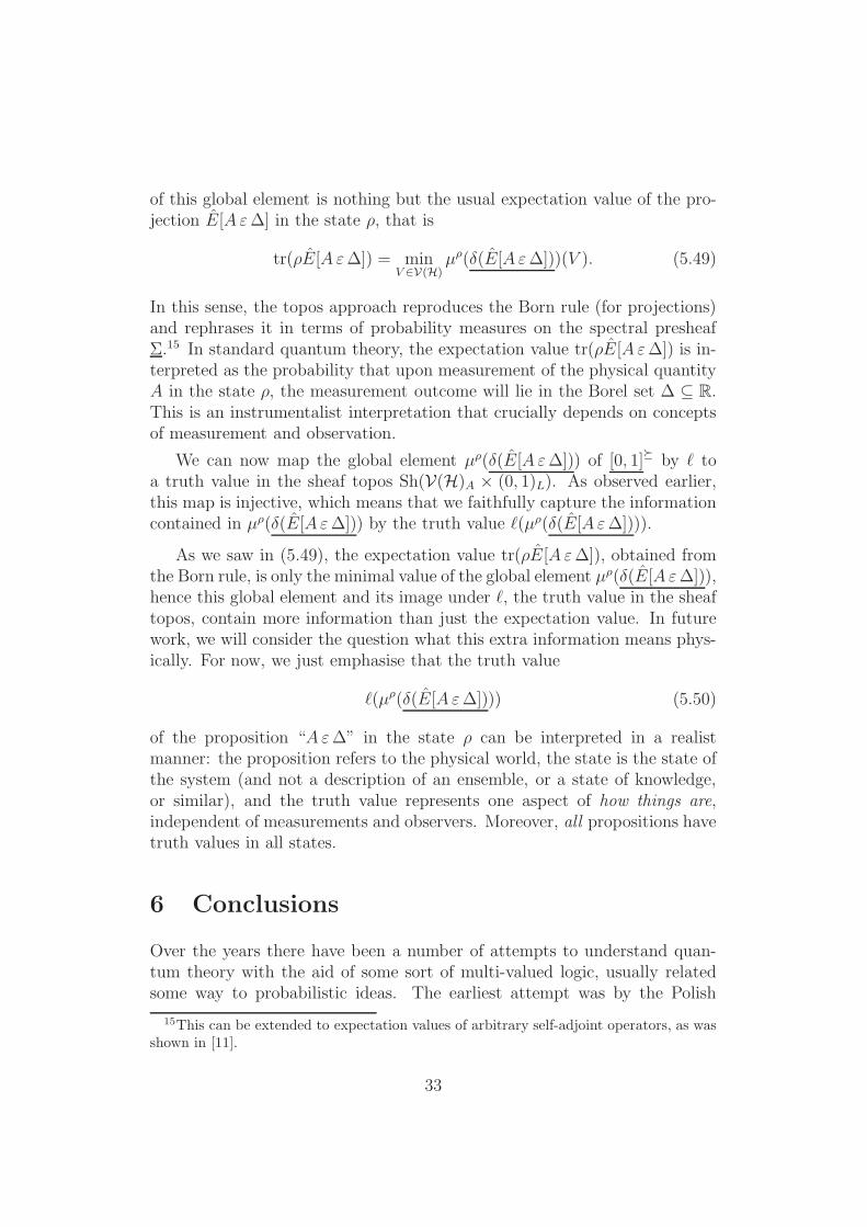
of this global element is nothing but the usual expectation value of the pro-jection E[Aε∆] in the state ρ, that is

tr(ρE[Aε∆]) = minV ∈V(H)

µρ(δ(E[Aε∆]))(V ). (5.49)

In this sense, the topos approach reproduces the Born rule (for projections)and rephrases it in terms of probability measures on the spectral presheafΣ.15 In standard quantum theory, the expectation value tr(ρE[Aε∆]) is in-terpreted as the probability that upon measurement of the physical quantityA in the state ρ, the measurement outcome will lie in the Borel set ∆ ⊆ R.This is an instrumentalist interpretation that crucially depends on conceptsof measurement and observation.

We can now map the global element µρ(δ(E[Aε∆])) of [0, 1] by ℓ toa truth value in the sheaf topos Sh(V(H)A × (0, 1)L). As observed earlier,this map is injective, which means that we faithfully capture the informationcontained in µρ(δ(E[Aε∆])) by the truth value ℓ(µρ(δ(E[Aε∆]))).

As we saw in (5.49), the expectation value tr(ρE[Aε∆]), obtained fromthe Born rule, is only the minimal value of the global element µρ(δ(E[Aε∆])),hence this global element and its image under ℓ, the truth value in the sheaftopos, contain more information than just the expectation value. In futurework, we will consider the question what this extra information means phys-ically. For now, we just emphasise that the truth value

ℓ(µρ(δ(E[Aε∆]))) (5.50)

of the proposition “Aε∆” in the state ρ can be interpreted in a realistmanner: the proposition refers to the physical world, the state is the state ofthe system (and not a description of an ensemble, or a state of knowledge,or similar), and the truth value represents one aspect of how things are,independent of measurements and observers. Moreover, all propositions havetruth values in all states.

6 Conclusions

Over the years there have been a number of attempts to understand quan-tum theory with the aid of some sort of multi-valued logic, usually relatedsome way to probabilistic ideas. The earliest attempt was by the Polish

15This can be extended to expectation values of arbitrary self-adjoint operators, as wasshown in [11].

33

mathematician Lukasiewicz [23] after whose work a number of philosophersof science have made a variety of proposals.

Much of this work involved three-valued logic, the most famous proponentof which was probably Reichenbach [20]. One problem commonly faced bysuch schemes is an uncertainty of how to define the logical connectives.

Lukasiewicz logic that is infinite-valued has also been studied, and thisincludes logics whose truth values lie in [0, 1]. This leads naturally to thesubject of fuzzy logic and fuzzy set theory. We refer the reader to the veryuseful review by Pykacz [22] which introduces the historical background tothese ideas. Another attempt to relate probability to logic is that of Carnapwhose work, like much else, has largely disappeared into the hazy past [21] .

Our topos approach is different to any of the existing schemes and, wewould claim, is better motivated and underpinned with very powerful math-ematical machinery. We have no problem defining logical connectives as thisstructure is given uniquely by the theory. That is, the propositional logic isgiven by the Heyting algebra Subcl(Σ), and the possible truth values belongto the Heyting algebra ΓΩ.

In the topos theory, truth values are not only multi-valued, they are alsocontextual in a way that is deeply tied to the underlying quantum theory.That explains why our probability measures are not simply [0, 1]-valued butare associated with arrows from Subcl(Σ) to (global elements of) the presheaf[0, 1].

In the present paper we make the strong claim that standard, classicalprobability theory can be faithfully represented by the global elements of thesub-object classifier, Ω(0,1), in the topos, Sh((0, 1)L), of sheaves on the topo-logical space (0, 1)L, whose open sets correspond bijectively to probabilitiesin the interval [0, 1]. This tight link between classical probability measuresand Heyting algebras is captured precisely in the commutative map diagramin (4.57). This approach to probability theory allows for a new type ofnon-instrumentalist interpretation that might be particularly appropriate in‘propensity’ schemes.

What, to us, is rather striking is that the same can be said about theinterpretation of probability in quantum theory. The relevant commutativediagram here is (5.40) which shows how our existing topos quantum theory,which uses the topos Sh(V(H)A), can be combined with our suggested toposapproach to probability, which uses the topos Sh((0, 1)L), to give a new toposquantum scheme which involves sheaves in the topos Sh(V(H)A × (0, 1)L).

As we have seen, in this scheme, results of quantum theory be codedin either (i) the topos probability measures µρ : Subcl(Σ) → [0, 1] (which

34

reinforces our slogan “Quantum physics is equivalent to classical physics inthe appropriate topos”); or (ii) the topos truth values, ν

(

Aε∆; ρ)

, defined

in (5.38), which take their values in the Heyting algebra ΓΩSh(V(H)A×(0,1)L).

Thus, in both classical and quantum physics, probability can be faithfullyinterpreted using truth values in sheaf topoi with an intuitionistic logic.

7 Appendix

We prove some technical results here.

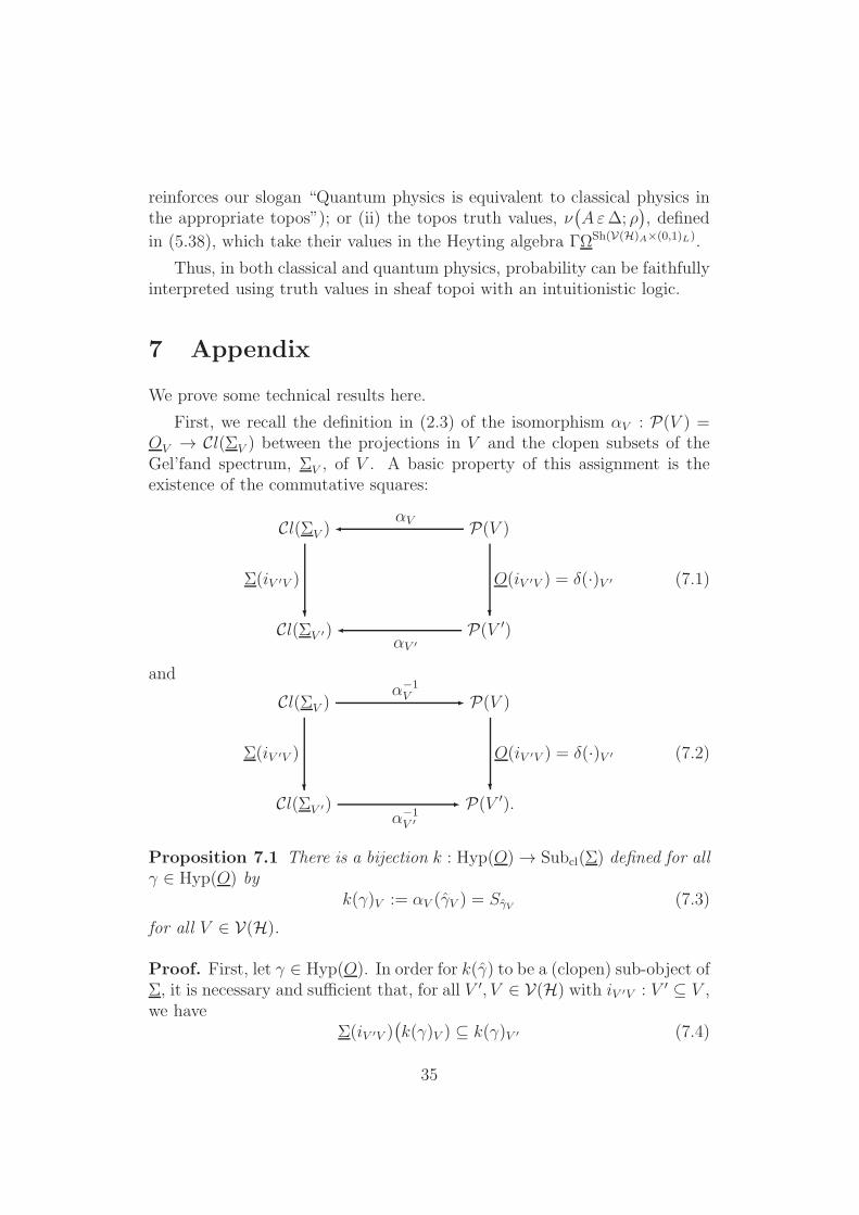
First, we recall the definition in (2.3) of the isomorphism αV : P(V ) =OV → Cl(ΣV ) between the projections in V and the clopen subsets of theGel’fand spectrum, ΣV , of V . A basic property of this assignment is theexistence of the commutative squares:

Cl(ΣV ) αV

P(V )

Cl(ΣV ′)

Σ(iV ′V )

?

αV ′

P(V ′)

O(iV ′V ) = δ(·)V ′

?

(7.1)

and

Cl(ΣV )α−1V - P(V )

Cl(ΣV ′)

Σ(iV ′V )

?

α−1V ′

- P(V ′).

O(iV ′V ) = δ(·)V ′

?

(7.2)

Proposition 7.1 There is a bijection k : Hyp(O) → Subcl(Σ) defined for allγ ∈ Hyp(O) by

k(γ)V := αV (γV ) = SγV (7.3)

for all V ∈ V(H).

Proof. First, let γ ∈ Hyp(O). In order for k(γ) to be a (clopen) sub-object ofΣ, it is necessary and sufficient that, for all V ′, V ∈ V(H) with iV ′V : V ′ ⊆ V ,we have

Σ(iV ′V )(

k(γ)V ) ⊆ k(γ)V ′ (7.4)

35

However, the commutative square in (7.1) gives

Σ(iV ′V )(Sα) = SO(iV ′V )(α) = Sδ(α)V ′ (7.5)

for all α ∈ OV and for all V, V ′ ∈ V(H) with iV ′V : V ′ ⊆ V . Because γ is ahyper-element of O we have δ(γV )V ′ γV ′, and hence

Σ(iV ′V )(

k(γ)V)

= Σ(iV ′V )(

SγV)

(7.6)

= Sδ(γV )V ′ ⊆ SγV ′ = k(γ)V ′ (7.7)

which proves (7.4), as required. Thus the map k in (7.3) defines a clopensub-object of Σ.

Conversely, define a map j : Subcl(Σ) → Hyp(O) by

j(S)V := α−1V (SV ) = PSV (7.8)

for all S ∈ Subcl(Σ) and for all V ∈ V(H). To check that the right handside of (7.8) is indeed a hyper-element of O, first note that the commutativesquare (7.2) gives

δ(j(S)V )V ′ = δ(PSV )V ′ = α−1V ′

(

Σ(iV ′V )(SV ))

(7.9)

However, since S is a sub-object of Σ, we have Σ(iV ′V )(SV ) ⊆ SV ′ , and so,from (7.9), for all V ′ ⊆ V ,

δ(j(S)V )V ′ α−1V ′ (SV ′) = PSV ′ = j(S)V ′ (7.10)

Thus the association V 7→ j(S)V does indeed define a hyper-element of O.

It is straightforward to show that the maps k : Hyp(O) → Subcl(Σ) andj : Subcl(Σ) → Hyp(O) are inverses of each. Thus the theorem is proved.

Proposition 7.2 There is a bijective correspondence

c : Sub(O) → Hyp(O) (7.11)

defined by

c(A)V :=∨

α | α ∈ AV (7.12)

for all sub-objects A of O.

Proof. The first step is to show that the right hand side of (7.12) is ahyper-element of O. To this end we note that, for any V ′ ⊆ V ,

δ(c(AV ))V ′ = δ(

∨

α ∈ AV )

V ′ =∨

δ(α)V ′ | α ∈ AV (7.13)

36

where we have used the fact that daseinisation commutes with the logical∨-operation. It is then clear that, since δ(α)V ′ | α ∈ AV ⊆ β | β ∈ AV ′,

δ(c(AV ))V ′ =∨

δ(α)V ′ | α ∈ AV ∨

β | β ∈ AV ′ = c(A)V ′ (7.14)

Therefore, the function V 7→ c(A)V defines a hyper-element of O, as required.

Conversely, define a function d : Hyp(O) → Sub(O) by

d(γ)V := α ∈ P(V ) | α γV (7.15)

for all V ∈ V(H). To show that the right hand side of (7.15) is a sub-objectof the outer presheaf, O, we first note that, for all V ′ ⊆ V ,

O(iV ′V )(

d(γ)V)

= δ(

α ∈ P(V ) | α γV )

V ′ = δ(α)V ′ | α γV (7.16)

Now, if α γV in P(V ) then δ(α)V ′ δ(γV )V ′ in P(V ′) and, because γ is ahyper-element, δ(γV )V ′ γV ′ . Therefore,

O(iV ′V )(

d(γ)V)

= δ(α)V ′ | α γV

⊆ δ(α)V ′ | δ(α)V ′ δ(γV )V ′

⊆ δ(α)V ′ | δ(α)V ′ γV ′

⊆ β ∈ P(V ′) | β γV ′ = d(γ)V ′ (7.17)

Thus d(γ) is a sub-object of O, as claimed. It is easy to check that c :Sub(O) → Hyp(O) and d : Hyp(O) → Sub(O) are inverses.

References

[1] C.J. Isham and J. Butterfield. A topos perspective on the Kochen-Specker theorem: I. Quantum states as generalised valuations. Int. J.Theor. Phys. 37, 2669–2733 (1998).

[2] C.J. Isham and J. Butterfield. A topos perspective on the Kochen-Specker theorem: II. Conceptual aspects, and classical analogues. Int.J. Theor. Phys. 38, 827–859 (1999).

[3] C.J. Isham, J. Hamilton and J. Butterfield. A topos perspective onthe Kochen-Specker theorem: III. Von Neumann algebras as the basecategory. Int. J. Theor. Phys. 39, 1413–1436 (2000).

[4] C.J. Isham and J. Butterfield. A topos perspective on the Kochen-Specker theorem: IV. Interval valuations. Int. J. Theor. Phys 41, 613–639 (2002).

37

[5] A. Doring, and C.J. Isham. A topos foundation for theories of physics:I. Formal languages for physics, J. Math. Phys 49, 053515 (2008).

[6] A. Doring, and C.J. Isham. A topos foundation for theories of physics:II. Daseinisation and the liberation of quantum theory. J. Math. Phys49, 053516 (2008).

[7] A. Doring, and C.J. Isham. A topos foundation for theories of physics:III. Quantum theory and the representation of physical quantities witharrows A : Σ → R. J. Math. Phys 49, 053517 (2008).

[8] A. Doring, and C.J. Isham. A topos foundation for theories of physics:IV. Categories of systems. J. Math. Phys 49, 053518 (2008).

[9] A. Doring. Topos theory and ‘neo-realist’ quantum theory. In Quan-tum Field Theory, Competitive Models, eds. B. Fauser, J. Tolksdorf, E.Zeidler, Birkhauser (2009).

[10] A. Doring, and C.J. Isham. ‘What is a Thing?’: Topos Theory in theFoundations of Physics. In New Structures for Physics, ed. B. Coecke,Lecture Notes in Physics 813, Springer, Berlin, Heidelberg (2010).

[11] A. Doring. Quantum states and measures on the spectral presheaf. Adv.Sci. Letts 2, 291–301 (2009).

[12] A. Doring. The Physical Interpretation of Daseinisation. To appear inDeep Beauty, ed. Hans Halvorson, Cambridge University Press (2011).

[13] C. Flori. A topos formulation of consistent histories. Jour. Math. Phys51 053527 (2009).

[14] C. Heunen, N.P. Landsman, and B. Spitters. The principle of gen-eral tovariance. Proceedings of the XVI International Fall Workshop onGeometry and Physics, Lisbon, 2007, eds. R. Picken et al., AmericanPhysical Society, 73–112 (2008).

[15] M. Caspers, C. Heunen, N.P. Landsman, and B. Spitters. Intuitionisticquantum logic of an n-level system. Found. Phys. 39, 731–759 (2009).

[16] C. Heunen, N.P. Landsman, and B. Spitters. A topos for algebraicquantum theory. Comm. Math. Phys. 291, 63–110 (2009).

[17] C. Heunen, N.P. Landsman, and B. Spitters. Bohrification of vonNeumann algebras and quantum logic. Synthese, in press (2010).arXiv:0905.2275.

38

[18] C. Heunen, N.P. Landsman, and B. Spitters. Bohrification. To appearin Deep Beauty, ed. H. Halvorson, Cambridge University Press (2011).

[19] C. Heunen, N.P. Landsman, B. Spitters, and S. Wolters. The Gelfandspectrum of a noncommutative C*-algebra: a topos-theoretic approach.Preprint, arXiv:1010.2050v1 (2010).

[20] H. Reichenbach. Philosophic Foundations of Quantum Mechanics. Uni-versity of California Press, Berkeley (1944).

[21] R. Carnap. Logical Foundations of Probability. Routledge and KeganPaul, London (1950).

[22] J. Pykacz. Quantum logic as partial infinite-valued Lukasiwicz logic.Int. Jour. Theor. Phys 34, 1697–1709 (1995).

[23] J. Lukasiewicz. Die logischen Grundlagen der Wahrscheinlichkeitsrech-nung, Akademie der Wissenschaften, Krakow (1913). [English transla-tion, Logical foundations of probability theory, in [24], pp. 16–63].

[24] J. Lukasiewicz. Selected Works. North-Holland, Amsterdam (1970).

39