Classical and Quantum Logic Gates

Classical and Quantum Logic Gates:An Introduction to Quantum Computing

Quantum Information Seminar

Friday, Sep. 3, 1999

Ashok Muthukrishnan

Rochester Center for Quantum Information (RCQI)

_____________________________________________________________

I. Classical Logic Gates

A. Irreversible Logic (1940-) ---------------------------------------------------- p. 2

1. Two-bit NAND gates simulate all Boolean functions2. Efficiency and the need for minimization techniques.

B. Reversible Logic (1970s) ----------------------------------------------------- p. 4

1. Minimizing energy-dissipation in a computation2. Three-bit Toffoli gates simulate all reversible Boolean functions

II. Quantum Logic Gates

A. Quantum vs. Classical Logic (1980s) -------------------------------------- p. 8

1. Bits and Boolean functions vs. Qubits and unitary matrices2. Classical reversible logic contained in quantum logic

B. Universal Quantum Logic Gates (1989, 1995-) ------------------------- p.12

1. Deutsch’s three-qubit generalization of the Toffoli gate2. Sufficiency of two-qubit gates for quantum computation3. Universality of two-qubit gates: proof sketch4. XOR gate: role in universality, entanglement, error-correction5. Implementation of two-qubit gates – the linear ion trap scheme

C. Multi-valued and continuous logic (1998-) ------------------------------ p.20

1. Multi-valued logic with qudits

2

I.A. Irreversible Classical Logic

Classical computation theory began for the most part when Church and Turing independently

published their inquiries into the nature of computability in 1936 [1]. For our purposes, it will

suffice to take as our model for classical discrete computation, a block diagram of the form,

a1

: f (a1, ... , an) b (1) an

where b = f (a1, a2, ... , an) describes a single-valued function on n discrete inputs. We will assume

that such a function can be simulated or computed physically. As is usually done in classical

computation, we can use base-2 arithmetic to describe the inputs and outputs, in which case

a1, ... , an, and b become binary variables, or bits, taking on one of two values, 0 or 1. In this case,

the function f (a1, a2, ... , an) is known as an n-bit Boolean function.

The central problem that we will concern ourselves with repeatedly in these notes is the problem

of universality. That is, given an arbitrarily large function f, is it possible to identify a universal

set of simple functions – called gates – that can be used repeatedly in sequence to simulate f on its

inputs. The gate functions would be restricted to operating on a small number of inputs, say two

or three at a time, taken from a1, a2, ... , an. These gates would be done in sequence, creating a

composite function that represents f on all of its n inputs.

It has been known for a long time that the two-bit gates, AND and OR, and the one-bit gate NOT,

are universal for classical computation, in the sense that they are sufficient to simulate any

function of the form illustrated in diagram (1). Gate functions in classical logic are often

represented using truth tables. The AND and OR gates have two inputs and one output, while the

NOT gate has one input and one output. A truth table lists all possible combinations of the input

bits and the corresponding output value for each gate.

a1 a2 a1 AND a2 a1 a2 a1 OR a2 a1 NOT a1

0 0 0 0 0 0 0 10 1 0 0 1 1 1 0 (2)1 0 0 1 0 11 1 1 1 1 1

The AND gate outputs 1 if and only if both inputs are 1, the OR gate outputs 1 if either or both

inputs are 1, and the NOT gate inverts the input. To illustrate that these three gates suffice to

3

build arbitrary Boolean functions, consider the three-bit Boolean function f(a1, a2, a3) given by a

truth table, whose first three lines look as follows,

a1 a2 a3 f(a1, a2, a3)

0 0 0 10 0 1 0 (3)0 1 0 1 : : : :

f has the output value 1 in the first line of its truth table. The function, f1 = (NOT a1) AND (NOT

a2) AND (NOT a3), also has the value 1 when a1 = 0, a2 = 0, and a3 = 0, but has the value 0 for all

other combinations of a1, a2, and a3. So f1 mimics the output of f, namely 1, for inputs taken from

the first line of the truth table for f. Similarly, we can construct functions that mimic f for each

line in the truth table for which f = 1. After the first line, f = 1 again in the third line of the truth

table. So for this line, we can construct the function f3 = (NOT a1) AND (a2) AND (NOT a3),

which has the value 1 when a1 = 0, a2 = 0, and a3 = 1. Since the functions f1, f3, ... are disjoint in

the sense that their 1-outputs correspond to distinct lines in the truth table, we can reconstruct f

for all the lines in the truth table by disjunctively combining all of the functions f1, f3, ...,

f = f1 OR f3 OR ... (4)

which are no more than eight in number in this case since there are eight lines in the truth table

for the three-bit function f. The expression on the right side of Eq. (4) is referred to in the texts as

the “disjunctive normal form” of the function f. Generalizing this procedure, we see that we can

simulate arbitrary Boolean functions using only the gates AND, OR, and NOT. So these three

gates are universal for classical Boolean logic. As a further simplification, these three gates can

be reduced to a single gate, the NAND gate,

a1 a2 a1 NAND a2

0 0 1a NAND b ≡ NOT (a AND b) 0 1 1 (5)

1 0 11 1 0

Representing the NAND operation by the symbol ↑ , it can be verified that

a OR b = (a ↑ a) ↑ (b ↑ b)

a AND b = (a ↑ b) ↑ (a ↑ b) (6)

NOT a = a ↑ a

Hence, we have the remarkable result that the two-bit NAND gate alone is sufficient for classical

Boolean logic. However, the procedure illustrated in Eq. (4) for decomposing a Boolean function

4

into two-bit gates, is inefficient. That is, the number of NAND gates needed to simulate a

function with n inputs this way would scale exponentially in n. This is essentially because an n-

bit Boolean function has 2n lines in its truth table. Various minimization techniques have been

discovered over the years – the Veitch-Karnaugh map and the Quine-McCluskey procedure are

two of these – that allow more sophisticated decompositions of a function than we have

illustrated, and which have proved invaluable to the design and implementation of circuits for

classical computation (see ref. [2] for a simple treatment of these methods).

I.B. Reversible Classical Logic

The first concerns about the reversibility of computation were raised in the 1970s. There were

two related issues, logical reversibility and physical reversibility, which were intimately

connected. Logical reversibility refers to the ability to reconstruct the input from the output of a

computation, or gate function. For instance, the NAND gate is explicitly irreversible, taking two

inputs to one output, while the NOT gate is reversible (it is its’ own inverse). The connection to

physical reversibilty is usually made as follows. Since the NAND gate has only one output, one

of its’ inputs has effectively been erased in the process, whose information has been irretrievably

lost. The change in entropy that we would associate with the lost of one bit of information is ln 2,

which, thermodynamically, corresponds to an energy increase of kT ln 2, where k is Boltzman’s

constant and T is the temperature. The heat dissipated during a process is usually taken to be a

sign of physical irreversibility, that the microscopic physical state of the system cannot be

restored exactly as it was before the process took place.

In the 70s, people were thus asking themselves two questions, which were related. One was

whether a computation can be done in a logically reversible fashion (unlike one that uses NAND

gates, for example), and the other was whether any heat needs to be dissipated during a

computation. Both of these issues were quite academic however, since as Feynman pointed out

[6], an actual transistor dissipates close to 1010 kT of heat, and even the DNA copying mechanism

in a human cell dissipates about 100 kT of heat per bit copied [which is understandable from a

consideration of the chemical bonds that need to be broken in the process], both far from the ideal

limit of kT ln 2 for irreversible computing.

That classical computation can be done reversibly with no energy dissipated per computational

step was discovered by Bennett in 1973 [3]. He showed this by constructing a reversible model

of the Turing machine – a symbolic model for computation introduced by Turing in 1936 [1] –

5

and showing that any problem that can be simulated on the original irreversible machine can also

be simulated with the same efficiency on the reversible model. The logical reversibility inherent

in the reversible model implied that an implementation of such a machine would also be

physically reversible. This started the search for physical models for reversible classical

computation, a review of which is given in [5].

Our model for reversible computaton will be similar to that of diagram (1), except that the

number of inputs and outputs of the function f will be the same, and f will be required to be a one-

to-one Boolean function. Likewise, we can pose the probem of universality as before, and ask for

a set of universal reversible logic gates that can simulate arbitrary reversible Boolean functions.

Since reversible logic gates are symmetric with respect to the number of inputs and outputs, we

can represent them in ways other than the truth table, that emphasizes this symmetry. We have

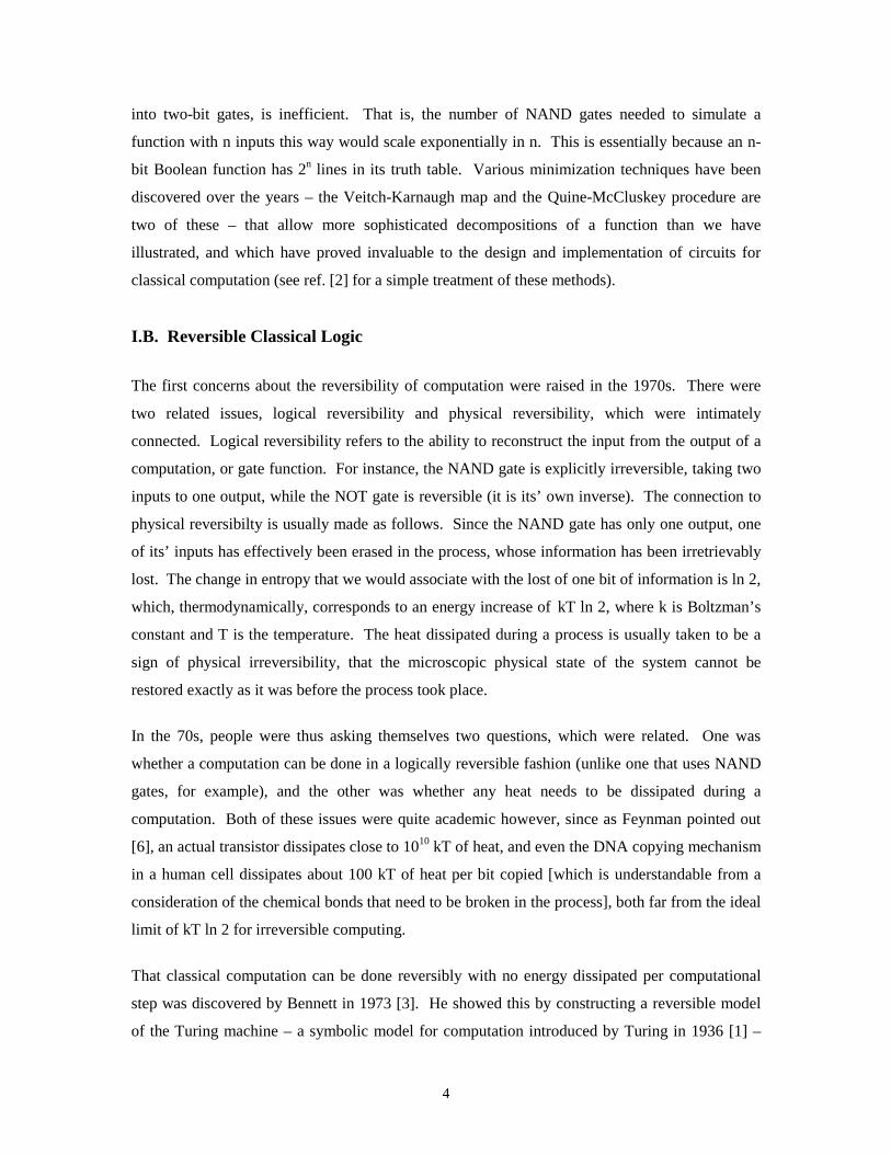
already encountered the reversible NOT gate, whose truth table was given in tables (2). We could

also write this in the form of a matrix, or as a graphic,

NOT ⟨0⟩ ⟨1⟩ ⟨0⟩ 0 1 a1 NOT a1 (7) ⟨1⟩ 1 0

The matrix form lists the lines in the truth table in the form ⟨0⟩ , ⟨1⟩ . The input lines are listed

horizontally on the top and the output lines are listed vertically along the side, in the same order.

We fill in the matrix with 1’s and 0’s such that each horizontal or vertical line has exactly one 1,

which is to be interpreted as a one-to-one mapping of the input to the output. For example, a 1 in

column one, row two in the NOT means that a ⟨0⟩ input gets taken to a ⟨1⟩ output. The graphical

representation to the right of the table in (7) is a condensed representation of the NOT gate. The

horizontal line represents a bit, whose initial variable value, a1, is listed on the left and whose

final value, NOT a1, is listed on the right. The operation of the NOT gate in the middle is

symbolised by the ⊕ sign. A two-bit gate closely related to the NOT gate is the two-bit

Controlled-NOT (or C-NOT) gate,

XOR = C-NOT ⟨00⟩ ⟨01⟩ ⟨ 10⟩ ⟨ 11⟩ ⟨00⟩ 1 0 0 0 a1 Χ a1

⟨01⟩ 0 1 0 0 (8) ⟨10⟩ 0 0 0 1 a2 a1 ⊕ a2

⟨11⟩ 0 0 1 0

which performs a NOT on the second bit if the first bit is ⟨1⟩ , but otherwise has no effect. The C-

NOT is sometimes also called XOR, since it performs an exclusive OR operation on the two input

6

bits and writes the output to the second bit. The graphical representation of this gate has two

horizontal lines representing the two variable bits, and the conditionality of the operation is

represented by the addition of a vertical line originating from the first bit and terminating with a

NOT symbol on the second bit. The Χ symbol on the first bit indicates that this bit is being

checked to see whether it is in ⟨1⟩ , before performing NOT on the second bit.

It turns out that classical reversible logic differs in one significant respect from classical

irreversible logic in that two-bit gates are not sufficient for universal reversible computation.

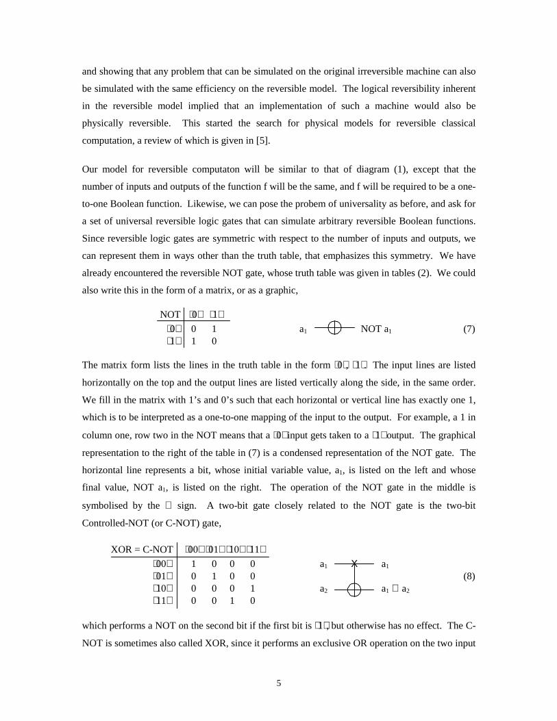
However, a three-bit gate is sufficient. A universal three-bit gate was identified by Toffoli [4] in

1981, called the Controlled-Controlled-NOT (or CC-NOT),

T3 = CC-NOT ⟨000⟩ ... ⟨110⟩ ⟨111⟩ ⟨000⟩ 1 0 0 0 0 0 0 0 (9) ⟨001⟩ 0 1 0 0 0 0 0 0 ⟨010⟩ 0 0 1 0 0 0 0 0 a1 Χ a1

⟨011⟩ 0 0 0 1 0 0 0 0 ⟨100⟩ 0 0 0 0 1 0 0 0 a2 Χ a2

⟨101⟩ 0 0 0 0 0 1 0 0 ⟨110⟩ 0 0 0 0 0 0 0 1 a3 a1a2 ⊕ a3

⟨111⟩ 0 0 0 0 0 0 1 0

or simply the three-bit Toffoli gate, T3. It applies a NOT to the third bit if the first two bits are in

⟨11⟩ , but otherwise having no effect. The graphical representation of this conditional three-bit

gate is given to the right of the table in (9), where both a1 and a2 are checked to see if they are in

⟨1⟩ - denoted by the two solid circles on these bits – before performing NOT on a3. The Toffoli

gate is known to be universal for reversible Boolean logic, the argument for which is based on the

fact that the Toffoli gate contains the NAND gate within it. When the third bit is fixed to be 1,

the Toffoli gate writes the NAND of the first two bits on the third, T3: a1, a2, 1 → a1, a2, a1↑ a2.

Lastly, we would like to consider why two-bit gates are not sufficient for reversible Boolean

logic. First note that the two-bit NAND gate cannot be made reversible without introducing a

third bit. If we were to retain one of the input bits in the output, and produce the NAND of the

two inputs in the second output bit, as this truth table illustrates,

a1 a2 a1 a1↑ a2

0 0 0 10 1 0 1 (10)1 0 1 11 1 1 0

7

the gate remains irreversible still, since the first two inputs are taken to the same output. To make

the NAND gate reversible, we really need to copy both the input bits into the output bit, and use a

third bit to store the result of the NAND operation, as is done in the Toffoli gate. To illustrate

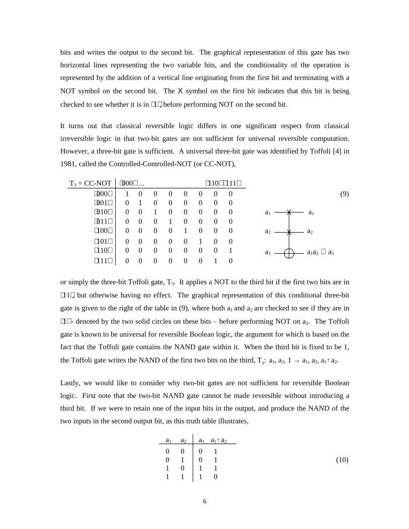
why three-bit gates are needed for decomposing reversible Boolean functions, consider writing

the four-bit CCC-NOT = T4 gate in terms of the three-bit Toffoli gates,

a1 Χ a1 Χ

a2 Χ a2 Χ =

a3 Χ a3 Χ (11)

a4 a4

⟨0⟩ Χ

where we have made use of an auxillary bit initialized to ⟨0⟩ , and the two gates on the right side

of the equation are performed from left to right. The gate on the left side is a four-bit gate that

applies NOT to the fourth bit when the first three bits are in ⟨111⟩ . The first Toffoli gate on the

right side checks the bits a1 and a2 to see if they are in ⟨11⟩ , and writes this information to the

single auxillary bit. The auxillary bit becomes ⟨1⟩ only when a1 and a2 are in ⟨11⟩ . The second

Toffoli gate collects this information from the auxillary bit, and conditional on this bit and the bit

a3, performs NOT on the bit a4, thus simulating the four-bit gate on the left side. The key feature

of the Toffoli gate that allowed this decomposition is its ability to condense the information from

two bits into one, something that cannot be accomplished by anything less than a three-bit gate.

One might think that the Toffoli gate T3 itself might be simulated by two two-bit C-NOTs (or

XORs), but as this example illustrates,

a1 Χ a1 Χ

a2 Χ ≠ a2 Χ (12)

a3 a3

such a simulation is not possible. The conditionality offered by the two XOR gates on the right

side is in an OR sense, where a NOT is performed on a3 when either a1 or a2 is in ⟨1⟩ , which is

distinct from the conditionality inherent in the Toffoli gate on the left side, where a NOT is

performed on a3 only when both a1 and a2 are in ⟨1⟩ . We will see later that while such a classical

decomposition of the Toffoli gate in Eq. (12) is impossible, a quantum decomposition is possible.

8

II.A. Quantum vs. Classical Logic

The first papers on quantum models for computation were published in the 1980s. Similar to the

research into reversible models, the motivation was mostly academic at the time, an exploration

of the ultimate limits of computation. The real payoff for quantum computing did not come until

1994, when Shor announced his quantum algorithm for factoring large numbers with an

efficiency unparalled by any classical algorithm preceding it [9]. The factoring problem is used

widely to encrypt messages in public key cryptography, which made the feasibility of quantum

computing an urgent issue in the years to follow.

The issues we will address in this section are the same as those that dogged early researchers in

quantum computing in the 80s, that of what constitutes a quantum model for computation, if such

a thing were possible, and whether there are qualitative differences between such a model and the

preceeding classical models for computaton. We will summarize below some of the key

conceptual discoveries that resulted from this research. A landmark paper on this subject, which

considered some of these issues as well as the existence of a quantum analog to the Turing

machine, was published in 1985 by Deutsch [7]. The two important issues to address when it

comes to building a computer model is that of storage and processing. That is, what will be the

memory units of our quantum computer, and how the information contained in them will be

processed to do the computation. This will give us an idea of what constraints are placed on the

kind of computations that can take place in this system.

The memory units of a classical discrete computer are usually taken as bits, two-valued classical

variables, as we saw earlier. By analogy, we consider a two-valued quantum variable, called a

qubit, which may be simulated by a two-level quantum system. Suppose the levels, or eigenstates

of the quantum variable, are labeled |0⟩ and |1⟩ . This has a direct correspondence with the

discrete states of a classical bit, 0 and 1. However, a qubit is a quantum state, and as such can be

in a superposition state also. That is, in addition to |0⟩ and |1⟩ , a qubit can exist more generally in

the state, c0|0⟩ + c1|1⟩ , where c0 and c1 are complex coefficients normalized to 1. This is the main

distinction between classical and quantum memory, in that even though a qubit has discrete

eigenstates, there is something analog about it also in the continuous range of superposition states

that it can take on. In fact, there are really an infinite number of states possible to a qubit, not just

two, although only two of these are orthogonal or linearly independent.

9

There is another aspect of quantum mechanics, namely measurement collapse, that affects how

the information is read out from a qubit. Even though a qubit can exist in an arbitrary

superposition state, a measurement on it will always find it in one of the two eigenstates, |0⟩ or

|1⟩ , according to the measurement postulate of quantum mechanics. This means that upon

measurement, a qubit loses its quantum character and reduces effectively to a bit. The

irreversibility of measurement has important consequences for quantum computation, as we will

see shortly.

If we have more than one qubit in our quantum system, we can express its state in terms of

product eigenstates. For example, a two-qubit system has the basis states, |00⟩ , |01⟩ , |10⟩ , |11⟩ ,

which are the quantum analogs of the input lines in the truth table for a classical logic gate.

Unlike classical bits however, two or more qubits can interfere with one another, creating a

macroscopically coherent superposition, of the form c00|00⟩ + c01|01⟩ + c10|10⟩ + c11|11⟩ . More

generally, n qubits will have 2n product eigenstates, or dimensions, in their Hilbert space. These

will form the computational basis of an n-qubit quantum computer.

It has been suggested that there are superficial similarities between a qubit and the classical nat,

the analog unit of memory used in classical continuous computation, since a qubit can also exist

in a continuous range of superposition states as we saw. There are a couple of important

differences between a qubit and a nat however. The first is that upon measurement, a qubit

always reduces to a bit, while a nat may retain its analog character after measurement. The more

substantive difference between the two has to do with entanglement. Entanglement is another

name for the quantum correlation between two observables. While a nat may be able to represent

products of a superpostion state of two qubits, of the form [c0|0⟩ 1 + c1|1⟩ 1] [c0′ |0⟩ 2 + c1′ |1⟩ 2], it

cannot fully represent entangled states like (1/√2) [ |01⟩ + |10⟩ ], where the state of one qubit is

determined by a measurement on the other. When the observables describing the two qubits are

classically distinguishable, or macroscopically seperated, measurement of entangled states

enables quantum nonlocality, an issue that has significance in fundamental quantum theory as

well as in some recent applications of quantum communication (like quantum teleportation).

Once we have establish the memory units of a quantum computer, the next question to address is

what constitutes the computation itself. That is, what kind of functions can be computed, or

problems solved, using quantum mechanics. We saw that in classical reversible computing, the

types of functions that can be computed are reversible Boolean functions, with equal numbers of

inputs and outputs. The identifying feature of a quantum transformation is that it has to be

10

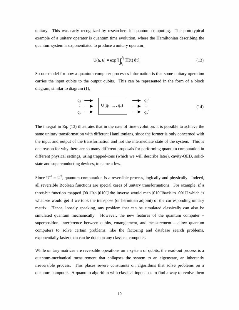
unitary. This was early recognized by researchers in quantum computing. The prototypical

example of a unitary operator is quantum time evolution, where the Hamiltonian describing the

quantum system is exponentiated to produce a unitary operator,

U(tf, ti) = exp ]dt H(t)i[ f

i

t

t∫ (13)

So our model for how a quantum computer processes information is that some unitary operation

carries the input qubits to the output qubits. This can be represented in the form of a block

diagram, similar to diagram (1),

q1 q1′: U (q1, ... , qn) : (14)

qn qn′

The integral in Eq. (13) illustrates that in the case of time-evolution, it is possible to achieve the

same unitary transformation with different Hamiltonians, since the former is only concerned with

the input and output of the transformation and not the intermediate state of the system. This is

one reason for why there are so many different proposals for performing quantum computation in

different physical settings, using trapped-ions (which we will describe later), cavity-QED, solid-

state and superconducting devices, to name a few.

Since U–1 = U†, quantum computation is a reversible process, logically and physically. Indeed,

all reversible Boolean functions are special cases of unitary transformations. For example, if a

three-bit function mapped |001⟩ to |010⟩ , the inverse would map |010⟩ back to |001⟩ , which is

what we would get if we took the transpose (or hermitian adjoint) of the corresponding unitary

matrix. Hence, loosely speaking, any problem that can be simulated classically can also be

simulated quantum mechanically. However, the new features of the quantum computer –

superposition, interference between qubits, entanglement, and measurement – allow quantum

computers to solve certain problems, like the factoring and database search problems,

exponentially faster than can be done on any classical computer.

While unitary matrices are reversible operations on a system of qubits, the read-out process is a

quantum-mechanical measurement that collapses the system to an eigenstate, an inherently

irreversible process. This places severe constraints on algorithms that solve problems on a

quantum computer. A quantum algorithm with classical inputs has to find a way to evolve them

11

into near-classical outputs again for efficient read-out, even though the intermediate state of the

system will be decidedly unclassical. This is achieved dramatically in Shor’s quantum algorithm

for factoring numbers.

The problem of universality can be posed for quantum computation as well, in asking whether

arbitrary unitary operations can be broken down into simpler ones. Similar to classical logic,

quantum logic gates exist that operate on a handful of qubits at a time, and that are able to

simulate arbitrary unitary operations. Note that it is a property of unitary matrices that a product

of two of them remains unitary, hence a product of unitary logic gates will also be unitary.

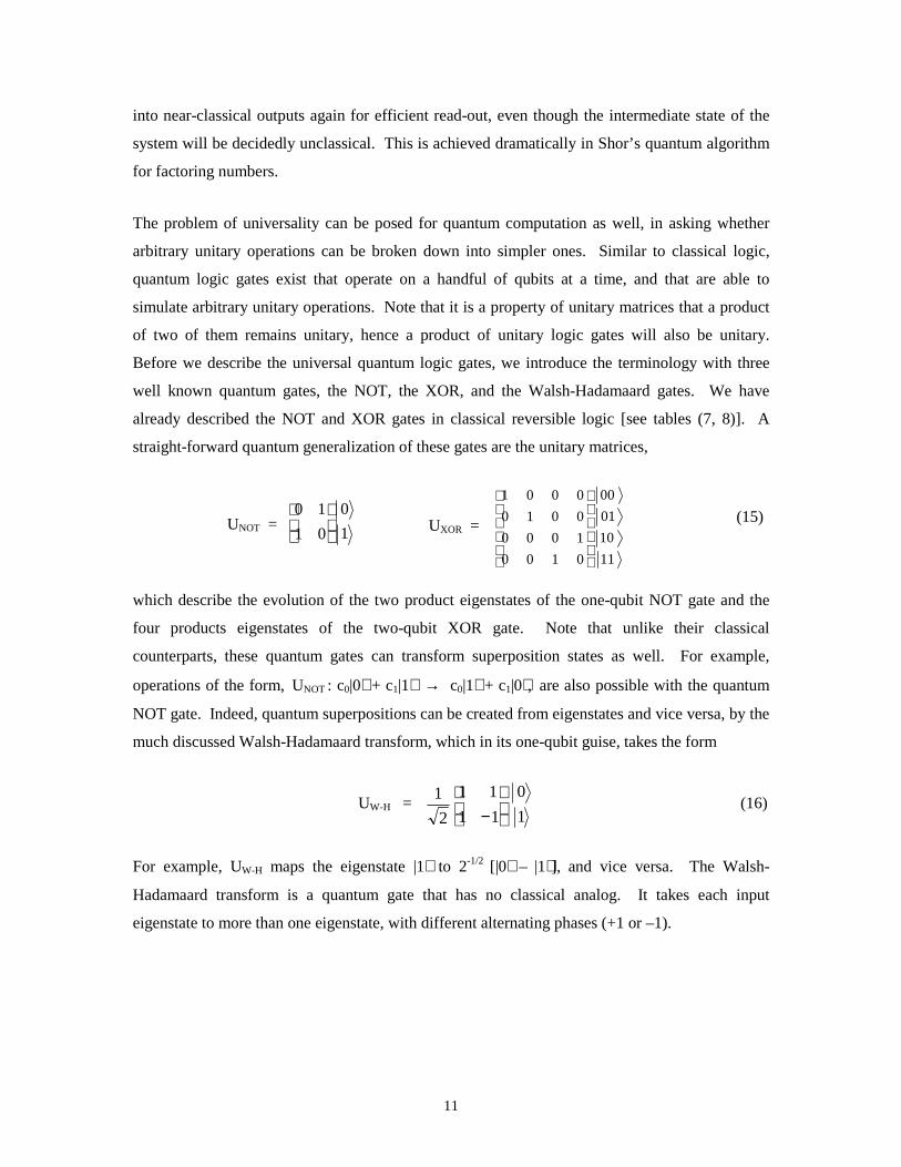
Before we describe the universal quantum logic gates, we introduce the terminology with three

well known quantum gates, the NOT, the XOR, and the Walsh-Hadamaard gates. We have

already described the NOT and XOR gates in classical reversible logic [see tables (7, 8)]. A

straight-forward quantum generalization of these gates are the unitary matrices,

UNOT = 1

0

01

10

UXOR =

11

10

01

00

0100

1000

0010

0001

(15)

which describe the evolution of the two product eigenstates of the one-qubit NOT gate and the

four products eigenstates of the two-qubit XOR gate. Note that unlike their classical

counterparts, these quantum gates can transform superposition states as well. For example,

operations of the form, UNOT : c0|0⟩ + c1|1⟩ → c0|1⟩ + c1|0⟩ , are also possible with the quantum

NOT gate. Indeed, quantum superpositions can be created from eigenstates and vice versa, by the

much discussed Walsh-Hadamaard transform, which in its one-qubit guise, takes the form

UW-H = 1

0

11

1 1

2

1

−

(16)

For example, UW-H maps the eigenstate |1⟩ to 2-1/2 [|0⟩ – |1⟩], and vice versa. The Walsh-

Hadamaard transform is a quantum gate that has no classical analog. It takes each input

eigenstate to more than one eigenstate, with different alternating phases (+1 or –1).

12

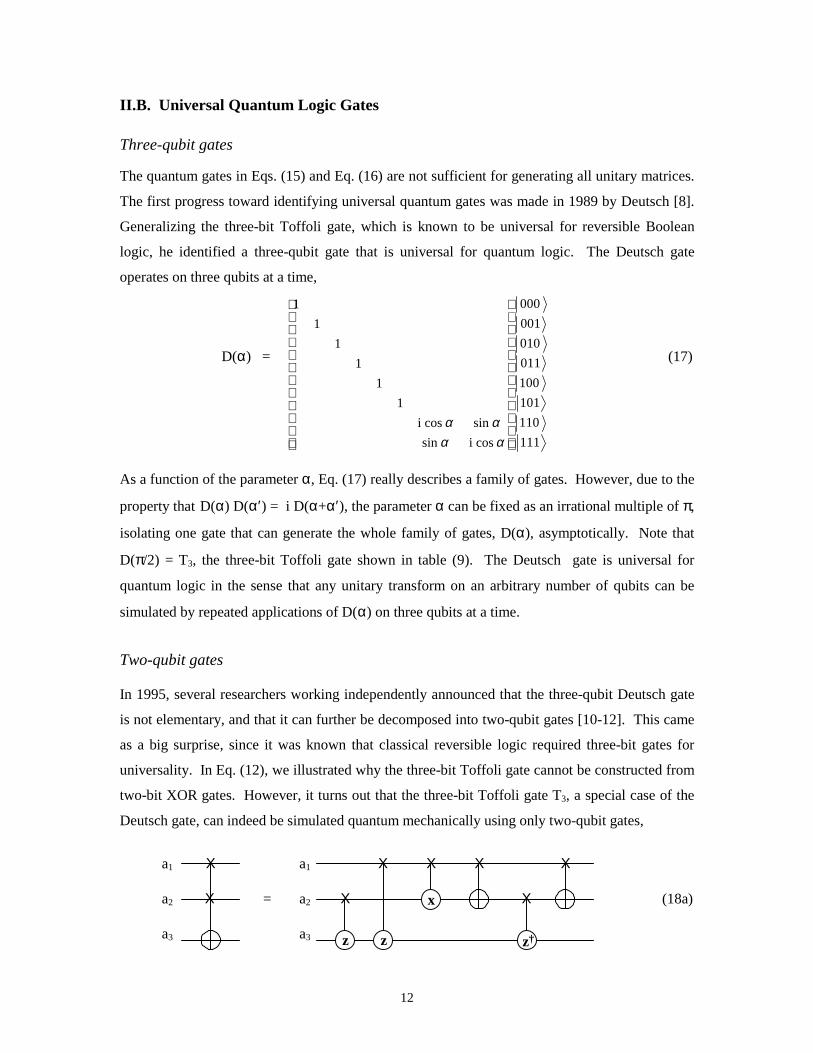
II.B. Universal Quantum Logic Gates

Three-qubit gates

The quantum gates in Eqs. (15) and Eq. (16) are not sufficient for generating all unitary matrices.

The first progress toward identifying universal quantum gates was made in 1989 by Deutsch [8].

Generalizing the three-bit Toffoli gate, which is known to be universal for reversible Boolean

logic, he identified a three-qubit gate that is universal for quantum logic. The Deutsch gate

operates on three qubits at a time,

D(α) =

111

110

101

100

011

010

001

000

cos isin

sincos i

1

1

1

1

1

1

αααα

(17)

As a function of the parameter α, Eq. (17) really describes a family of gates. However, due to the

property that D(α) D(α′ ) = i D(α+α′ ), the parameter α can be fixed as an irrational multiple of π,

isolating one gate that can generate the whole family of gates, D(α), asymptotically. Note that

D(π/2) = T3, the three-bit Toffoli gate shown in table (9). The Deutsch gate is universal for

quantum logic in the sense that any unitary transform on an arbitrary number of qubits can be

simulated by repeated applications of D(α) on three qubits at a time.

Two-qubit gates

In 1995, several researchers working independently announced that the three-qubit Deutsch gate

is not elementary, and that it can further be decomposed into two-qubit gates [10-12]. This came

as a big surprise, since it was known that classical reversible logic required three-bit gates for

universality. In Eq. (12), we illustrated why the three-bit Toffoli gate cannot be constructed from

two-bit XOR gates. However, it turns out that the three-bit Toffoli gate T3, a special case of the

Deutsch gate, can indeed be simulated quantum mechanically using only two-qubit gates,

a1 Χ a1 Χ Χ Χ Χ

a2 Χ = a2 Χ x Χ (18a)

a3 a3 z z z†

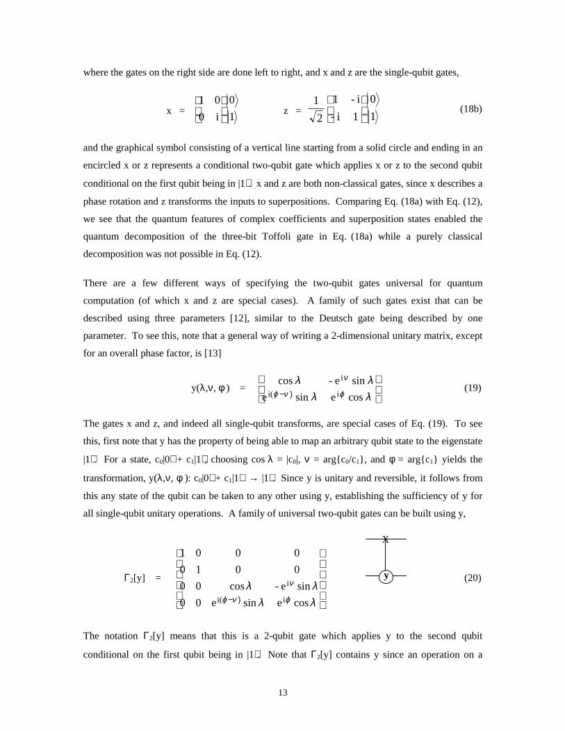
13

where the gates on the right side are done left to right, and x and z are the single-qubit gates,

x = 1

0

i0

01

z =

1

0

1i-

i-1

2

1

(18b)

and the graphical symbol consisting of a vertical line starting from a solid circle and ending in an

encircled x or z represents a conditional two-qubit gate which applies x or z to the second qubit

conditional on the first qubit being in |1⟩ . x and z are both non-classical gates, since x describes a

phase rotation and z transforms the inputs to superpositions. Comparing Eq. (18a) with Eq. (12),

we see that the quantum features of complex coefficients and superposition states enabled the

quantum decomposition of the three-bit Toffoli gate in Eq. (18a) while a purely classical

decomposition was not possible in Eq. (12).

There are a few different ways of specifying the two-qubit gates universal for quantum

computation (of which x and z are special cases). A family of such gates exist that can be

described using three parameters [12], similar to the Deutsch gate being described by one

parameter. To see this, note that a general way of writing a 2-dimensional unitary matrix, except

for an overall phase factor, is [13]

y(λ,ν, φ ) =

)− λλ

λλϕνϕ

ν

cosesine

sine-cos i i(

i (19)

The gates x and z, and indeed all single-qubit transforms, are special cases of Eq. (19). To see

this, first note that y has the property of being able to map an arbitrary qubit state to the eigenstate

|1⟩ . For a state, c0|0⟩ + c1|1⟩ , choosing cos λ = |c0|, ν = arg{c0/c1}, and φ = arg{c1} yields the

transformation, y(λ,ν, φ ): c0|0⟩ + c1|1⟩ → |1⟩ . Since y is unitary and reversible, it follows from

this any state of the qubit can be taken to any other using y, establishing the sufficiency of y for

all single-qubit unitary operations. A family of universal two-qubit gates can be built using y,

X

Γ2[y] =

)− λλλλ

ϕνϕ

ν

cosesine00

sine-cos00

0010

0001

i i(

i y (20)

The notation Γ2[y] means that this is a 2-qubit gate which applies y to the second qubit

conditional on the first qubit being in |1⟩ . Note that Γ2[y] contains y since an operation on a

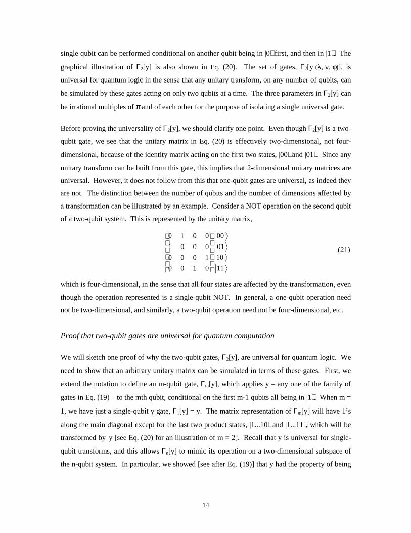
14

single qubit can be performed conditional on another qubit being in |0⟩ first, and then in |1⟩ . The

graphical illustration of Γ2[y] is also shown in Eq. (20). The set of gates, Γ2[y (λ, ν, φ)], is

universal for quantum logic in the sense that any unitary transform, on any number of qubits, can

be simulated by these gates acting on only two qubits at a time. The three parameters in Γ2[y] can

be irrational multiples of π and of each other for the purpose of isolating a single universal gate.

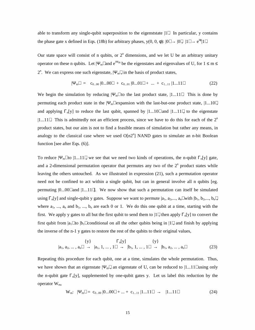
Before proving the universality of Γ2[y], we should clarify one point. Even though Γ2[y] is a two-

qubit gate, we see that the unitary matrix in Eq. (20) is effectively two-dimensional, not four-

dimensional, because of the identity matrix acting on the first two states, |00⟩ and |01⟩ . Since any

unitary transform can be built from this gate, this implies that 2-dimensional unitary matrices are

universal. However, it does not follow from this that one-qubit gates are universal, as indeed they

are not. The distinction between the number of qubits and the number of dimensions affected by

a transformation can be illustrated by an example. Consider a NOT operation on the second qubit

of a two-qubit system. This is represented by the unitary matrix,

11

10

01

00

0100

1000

0001

0010

(21)

which is four-dimensional, in the sense that all four states are affected by the transformation, even

though the operation represented is a single-qubit NOT. In general, a one-qubit operation need

not be two-dimensional, and similarly, a two-qubit operation need not be four-dimensional, etc.

Proof that two-qubit gates are universal for quantum computation

We will sketch one proof of why the two-qubit gates, Γ2[y], are universal for quantum logic. We

need to show that an arbitrary unitary matrix can be simulated in terms of these gates. First, we

extend the notation to define an m-qubit gate, Γm[y], which applies y – any one of the family of

gates in Eq. (19) – to the mth qubit, conditional on the first m-1 qubits all being in |1⟩ . When m =

1, we have just a single-qubit y gate, Γ1[y] = y. The matrix representation of Γm[y] will have 1’s

along the main diagonal except for the last two product states, |1...10⟩ and |1...11⟩ , which will be

transformed by y [see Eq. (20) for an illustration of m = 2]. Recall that y is universal for single-

qubit transforms, and this allows Γn[y] to mimic its operation on a two-dimensional subspace of

the n-qubit system. In particular, we showed [see after Eq. (19)] that y had the property of being

15

able to transform any single-qubit superposition to the eigenststate |1⟩ . In particular, y contains

the phase gate x defined in Eqs. (18b) for arbitrary phases, y(0, 0, φ): |0⟩ → |0⟩ , |1⟩ → eiφ |1⟩ .

Our state space will consist of n qubits, or 2n dimensions, and we let U be an arbitrary unitary

operator on these n qubits. Let |Ψm⟩ and eiΨm be the eigenstates and eigenvalues of U, for 1 ≤ m ≤

2n. We can express one such eigenstate, |Ψm⟩ , in the basis of product states,

|Ψm⟩ = c0...00 |0...00⟩ + c0...01 |0...01⟩ + ... + c1...11 |1...11⟩ (22)

We begin the simulation by reducing |Ψm⟩ to the last product state, |1...11⟩ . This is done by

permuting each product state in the |Ψm⟩ expansion with the last-but-one product state, |1...10⟩ ,

and applying Γn[y] to reduce the last qubit, spanned by |1...10⟩ and |1...11⟩ , to the eigenstate

|1...11⟩ . This is admittedly not an efficient process, since we have to do this for each of the 2n

product states, but our aim is not to find a feasible means of simulation but rather any means, in

analogy to the classical case where we used O[n2n] NAND gates to simulate an n-bit Boolean

function [see after Eqs. (6)].

To reduce |Ψm⟩ to |1...11⟩ , we see that we need two kinds of operations, the n-qubit Γn[y] gate,

and a 2-dimensional permutation operator that permutes any two of the 2n product states while

leaving the others untouched. As we illustrated in expression (21), such a permutation operator

need not be confined to act within a single qubit, but can in general involve all n qubits [eg.

permuting |0...00⟩ and |1...11⟩]. We now show that such a permutation can itself be simulated

using Γn[y] and single-qubit y gates. Suppose we want to permute |a1, a2,..., an⟩ with |b1, b2,..., bn⟩ ,

where a1, ..., an and b1, ..., bn are each 0 or 1. We do this one qubit at a time, starting with the

first. We apply y gates to all but the first qubit to send them to |1⟩ , then apply Γn[y] to convert the

first qubit from |a1⟩ to |b1⟩ conditional on all the other qubits being in |1⟩ , and finish by applying

the inverse of the n-1 y gates to restore the rest of the qubits to their original values,

{y} Γn[y] {y}|a1, a2, ... , an⟩ → |a1, 1, ... , 1⟩ → |b1, 1, ... , 1⟩ → |b1, a2, ... , an⟩ (23)

Repeating this procedure for each qubit, one at a time, simulates the whole permutation. Thus,

we have shown that an eigenstate |Ψm⟩ , an eigenstate of U, can be reduced to |1...11⟩ using only

the n-qubit gate Γn[y], supplemented by one-qubit gates y. Let us label this reduction by the

operator Wm,

Wm: |Ψm⟩ = c0...00 |0...00⟩ + ... + c1...11 |1...11⟩ → |1...11⟩ (24)

16

Wm is contained in Γn[y]. Similarly, the n-qubit phase gate,

Xm = Γn[y(0, 0, Ψm)]: |1...11⟩ → eiΨm |1...11⟩ (25)

where is the eigenphase of U corresponding to |Ψm⟩ , is also contained in Γn[y]. Now following an

argument by Deutsch [8], we consider the combination of transforms, Wm† Xm Wm, and show that

Wm† Xm Wm maps |Ψm⟩ to eiΨm |Ψm⟩ , and |Ψm′⟩ to |Ψm′⟩ for m′≠ m. First, when m′= m, we know

that Xm Wm maps |Ψm⟩ to eiΨm |1...11⟩ . Since Wm is unitary, this means that Wm† = Wm

-1 maps

|1...11⟩ to |Ψm⟩ . When m′≠ m, note that

⟨1...11| Wm |Ψm′⟩ = ⟨Ψm | Wm† Wm |Ψm′⟩ = ⟨Ψm | Ψm′⟩ = 0 (26)

where we have used the unitarity of Wm to recognize Wm† Wm as the identity, and the

orthogonality of {|Ψm⟩}. Eq. (26) shows that Wm |Ψm′⟩ has no component along |1...11⟩ , which

means that Xm will not affect this state. Hence Wm† Xm Wm |Ψm′⟩ = Wm

† Wm |Ψm′⟩ = |Ψm′⟩ when

m′= m. Since Wm† Xm Wm acts as an identity to all states |Ψm′⟩ except for m′= m , we have that

2n

2n

Π (Wm† Xm Wm) = ∑ eiΨm |Ψm⟩ ⟨Ψm | = U (27)

m = 1 m = 1

expressing that the product operator on the left shares the same eigenvectors and eigenvalues, and

hence must be the same as, U. Since Wm and Xm are contained in Γn[y], we have that Γn[y]

simulates U.

It remains to show that the n-qubit Γn[y] gates can be simulated with the two-qubit gates, Γ2[y].

We do this by showing that Γn[y (λ, ν, φ)], can be written in terms of Γ2[y (λ, ν, φ)] and the n-bit

version of the Toffoli gate, Tn = Γn[y(π/2, π, π)], which applies a NOT to the nth qubit when the

first n-1 qubits are in |1⟩ . Since Tn is a Boolean gate, we know that it can be reduced to the three-

bit Toffoli gate T3, which is univeral for classical reversible logic [see section I.B], and we have

already shown [see Eq. (18a)] that T3 is contained in Γ2[y]. We now show how Γn[y] can be built

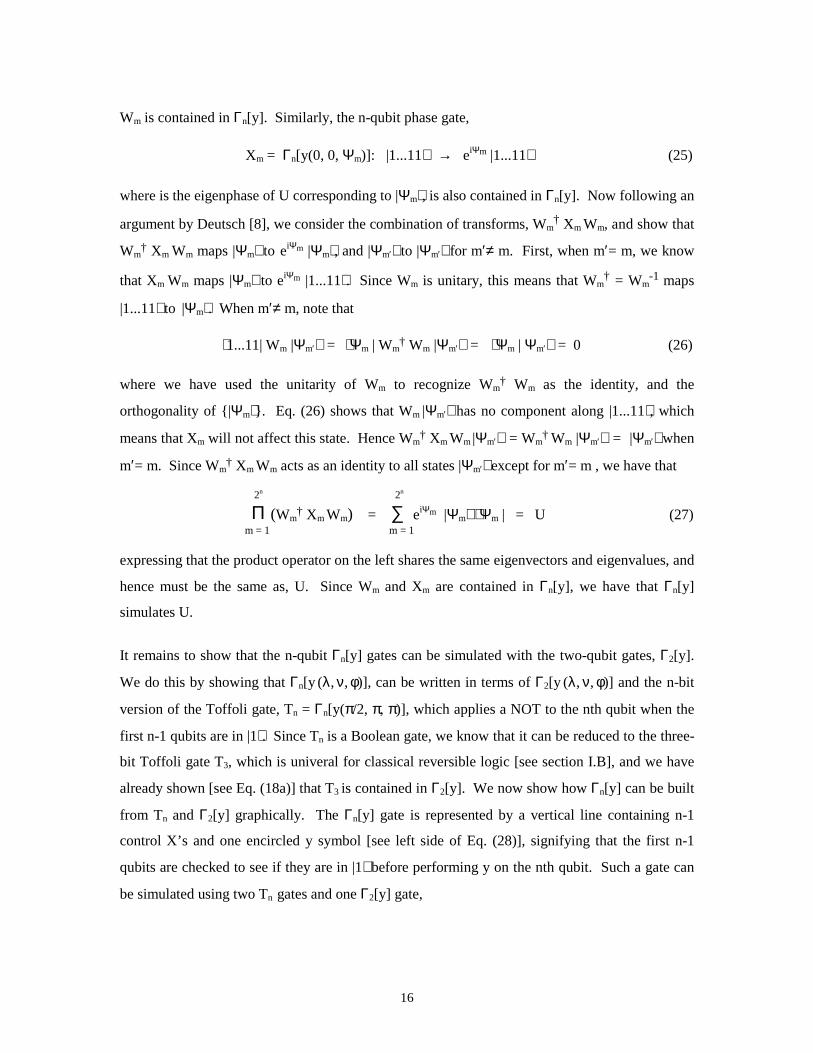
from Tn and Γ2[y] graphically. The Γn[y] gate is represented by a vertical line containing n-1

control X’s and one encircled y symbol [see left side of Eq. (28)], signifying that the first n-1

qubits are checked to see if they are in |1⟩ before performing y on the nth qubit. Such a gate can

be simulated using two Tn gates and one Γ2[y] gate,

17

1 Χ 1 Χ Χ

2 Χ 2 Χ Χ

= (28)

n-1 Χ n-1 Χ Χ

n y n y

|0⟩ Χ |0⟩

where the dashed horizontal line represents an auxillary qubit which is initialized to |0⟩ and is

returned to |0⟩ at the end. The first Toffoli gate Tn on the right side checks the first n-1 qubits to

see if they are in |1⟩ and stores this result in the auxillary qubit by converting it to |1⟩

conditionally. The two-bit Γ2[y] gate that follows collects this information from the auxillary

qubit and performs y on the nth qubit conditionally. The last Tn is to restore the auxillary qubit to

|0⟩ for possible re-use.

Properties of the XOR gate

Before considering how two-qubit gates may be implemented physically in the laboratory, we

emphasize the importance of one of these gates, the XOR gate, shown in table (8) and Eqs. (15).

The XOR gate is useful not only for its quantum logic properties but also for its use in quantum

error correction and teleportation. Note that the XOR gate is a special case of the universal two-

qubit family of gates, UXOR = Γ2[y(π/2, π, π)]. It performs a C-NOT operation, and is the two-bit

version of the three-bit Toffoli gate, UXOR = T2. The properties of the XOR gate that we describe

below are summarized in ref. [15]

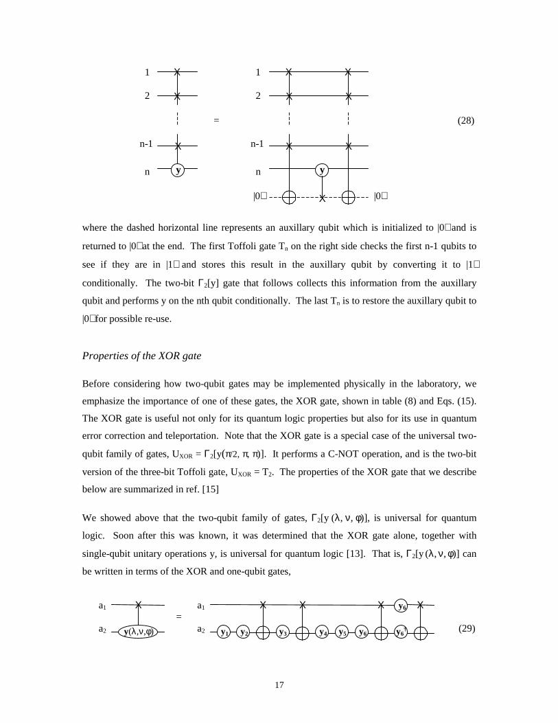
We showed above that the two-qubit family of gates, Γ2[y (λ, ν, φ)], is universal for quantum

logic. Soon after this was known, it was determined that the XOR gate alone, together with

single-qubit unitary operations y, is universal for quantum logic [13]. That is, Γ2[y (λ, ν, φ)] can

be written in terms of the XOR and one-qubit gates,

a1 Χ a1 Χ Χ Χ y6 Χ =

a2 y(λ,ν,φ) a2 y1 y2 y3 y4 y5 y6 y6† (29)

18

where y1 = y(π/2, π, 0), y2 = y(π/2,−ν/2, 0), y3 = y(−λ/2, 0, 0), y4 = y((λ−π)/2, 0, 0), y5 = y(π/2, ν/2, 0),

and y6 = y(0, 0, φ/2). This reduces the constraints on implementing a quantum computer physically

since the only two-qubit operation that needs to be performed is the XOR gate, which is much

simpler than the Γ2[y (λ, ν, φ)] gates.

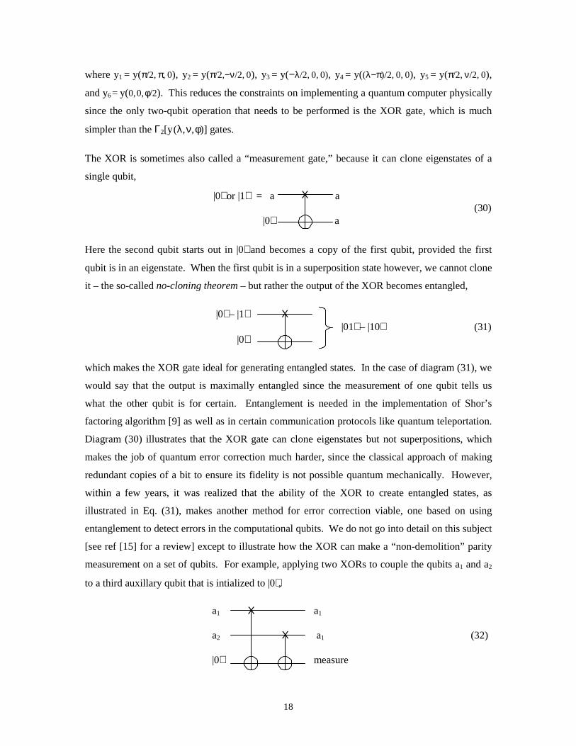
The XOR is sometimes also called a “measurement gate,” because it can clone eigenstates of a

single qubit,

|0⟩ or |1⟩ = a Χ a (30)

|0⟩ a

Here the second qubit starts out in |0⟩ and becomes a copy of the first qubit, provided the first

qubit is in an eigenstate. When the first qubit is in a superposition state however, we cannot clone

it – the so-called no-cloning theorem – but rather the output of the XOR becomes entangled,

|0⟩ – |1⟩ Χ |01⟩ – |10⟩ (31)

|0⟩

which makes the XOR gate ideal for generating entangled states. In the case of diagram (31), we

would say that the output is maximally entangled since the measurement of one qubit tells us

what the other qubit is for certain. Entanglement is needed in the implementation of Shor’s

factoring algorithm [9] as well as in certain communication protocols like quantum teleportation.

Diagram (30) illustrates that the XOR gate can clone eigenstates but not superpositions, which

makes the job of quantum error correction much harder, since the classical approach of making

redundant copies of a bit to ensure its fidelity is not possible quantum mechanically. However,

within a few years, it was realized that the ability of the XOR to create entangled states, as

illustrated in Eq. (31), makes another method for error correction viable, one based on using

entanglement to detect errors in the computational qubits. We do not go into detail on this subject

[see ref [15] for a review] except to illustrate how the XOR can make a “non-demolition” parity

measurement on a set of qubits. For example, applying two XORs to couple the qubits a1 and a2

to a third auxillary qubit that is intialized to |0⟩ ,

a1 Χ a1

a2 Χ a1 (32)

|0⟩ measure

19

and subsequently measuring this auxillary qubit, we can force the state of a1 and a2 to having

components only along even (or odd) product states. For example, the above two XORs

transform (33)

[c00 |00⟩ + c01 |01⟩ + c10 |10⟩ + c11 |11⟩ ] |0⟩ aux → [c00 |00⟩ + c11 |11⟩ ] |0⟩ aux + [c01 |01⟩ + c10 |10⟩ ] |1⟩ aux

where the value of the auxillary qubit at the end labels the parity of the comptational states. Such

a parity-measurement is “non-demolitional” only in the sense that the coherence within a basis of

a given parity is unaffected by the measurement of the auxillary qubit. This gives a sense of why

the XOR is useful in quantum error correction routines, where the coherence of the computational

qubits that we are correcting should not be affected by direct measurement.

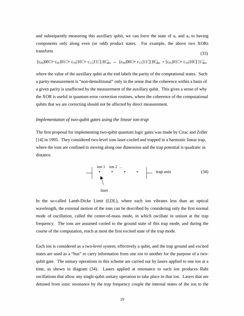
Implementaton of two-qubit gates using the linear ion-trap

The first proposal for implementing two-qubit quantum logic gates was made by Cirac and Zoller

[14] in 1995. They considered two-level ions laser-cooled and trapped in a harmonic linear trap,

where the ions are confined to moving along one dimension and the trap potential is quadratic in

distance.

ion 1 ion 2 ...• • • • trap axis (34)

laser

In the so-called Lamb-Dicke Limit (LDL), where each ion vibrates less than an optical

wavelength, the external motion of the ions can be described by considering only the first normal

mode of oscillation, called the center-of-mass mode, in which oscillate in unison at the trap

frequency. The ions are assumed cooled to the ground state of this trap mode, and during the

course of the computation, reach at most the first excited state of the trap mode.

Each ion is considered as a two-level system, effectively a qubit, and the trap ground and excited

states are used as a “bus” to carry information from one ion to another for the purpose of a two-

qubit gate. The unitary operations in this scheme are carried out by lasers applied to one ion at a

time, as shown in diagram (34). Lasers applied at resonance to each ion produces Rabi

oscillations that allow any single-qubit unitary operation to take place in that ion. Lasers that are

detuned from ionic resonance by the trap frequency couple the internal states of the ion to the

20

external trap states of all the ions. This coupling takes place if the laser field has spatial

dependence, as in the case of standing-wave field, and the ion’s dipole moment couples to the

field amplitude, which in turn depends on the position of the ion in the trap. Two-qubit

operations are achieved in this scheme in two stages, first entangling the internal states of one ion

with the trap states using a detuned standing-wave laser, and then transferring this information

from the trap to the second ion by a similar field applied to it.

II.C. Multi-valued Quantum Logic [For the continuous case, see [18, 19]]

Very recently, some progress has been made [16, 17] in generalizing quantum logic operations to

the multi-valued domain, where the fundamental memory units are no longer two-state qubits, but

rather d-valued qudits. Although a qudit can be said to have the same information as log2d

qubits, since they span the same Hilbert space, the measurement of a qudit is assumed to yield

only one value, not log2d values, corresponding to the eigenstate that the d-level quantum system

collapsed to.

The main motivation for making the transition from binary to multi-valued quantum logic is to

avail of the greater information capacity of multi-level atomic systems. Using more than two

levels in each ion in the linear ion trap scheme for example, we could reduce the number of ions

needed to be stored in the trap. This is an advantage because the bottleneck for implementing this

scheme, and in many others, is the maintenance of a macroscopically coherent state of all the ions

for a sufficiently long time before, subject to environmental noise, the coherence vanishes and the

computation is corrupted. Another difference between binary and multi-valued logic that applies

equally well to the classical and quantum domains is the trade-off in processing time – executing

a large number of small (2 or 4-dim) binary gates versus a small number of large (d or d2-dim)

multi-valued gates. If large single-qubit operations are more viable than doing many small ones

in sequence, then the multi-valued case will have an advantage.

The problem of universality has been addressed in the multi-valued domain [16] and it has been

found that similar to the binary case, two-qudit operations suffice for performing arbitrary unitary

operations on any number of qudits. Fault-tolerant error correction schemes have also been

advanced for multi-valued quantum logic [17].

21

References:

[1] A. Turing, “On computable numbers with an application to the Entscheidungs-problem,”Proc. Lond. Math. Soc. Ser. 2, 42 (1936), 230-65. Also see A. Church, “An unsolvableproblem of elementary number theory,” American J. of Math., 58 (1936), 345-63.[First inquiries into the nature of computability in classical discrete computation.]

[2] F. E. Hohn, Applied Boolean Algebra – An Elementary Introduction, The MacmillanCompany, New York, 1966.[Simple review of the classical logic gates and their semiconductor implementation.]

[3] C. H. Bennett, “Logical Reversibility of Computation,” IBM Journal of Research andDevelopment, 17 (1973), 525-32.[Using the language of Turing machines, showed that computation can be made reversible, with noenergy dissipated per step.]

[4] T. Toffoli, “Reversible Computing,” Tech. Memo MIT/LCS/TM-151, MIT Lab. for Com.Sci. (1980).[Showed that three-bit gates are universal for classical reversible computing.]

[5] C. H. Bennett, “The Thermodynamics of Computation – A Review,” Int. J. TheoreticalPhysics, 21 No. 12 (1982), 905-40.[Review of proposed physical models for reversible computing.]

[6] R. P. Feynman, “Quantum mechanical computers,” Found. Phys., 16 (1986), 507.[Review of work in classical reversible computing, and consideration of quantum extensions.]

[7] D. Deutsch, “Quantum theory, the Church-Turing principle and the universal quantumcomputer,” Proc. Roy. Soc. Lond. A, 400 (1985), 97-117.[First thorough description of a quantum model for computation.]

[8] D. Deutsch, “Quantum computational networks,” Proc. Roy. Soc. Lond. A, 425 (1989), 73-90.[Proof that three-qubit gates are universal for quantum computation.]

[9] P. Shor, “Algorithms for quantum computation: discrete log and factoring,” Proc. 35th AnnualSymp. on Found. of Computer Science (1994), IEEE Computer Society, Los Alamitos,124-34.[First algorithm to show that quantum computing was intrinsically more powerful than classicalcomputing, in the solution of the factoring problem.]

[10] D. P. DiVincenzo, “Two-bit gates are universal for quantum computation,” Phys. Rev. A,51 (1995), 1015-18.[First existence proof that two-qubit gates are universal for quantum computation.]

[11] T. Sleator, H. Weinfurter, “Realizable Universal Quantum Logic Gates,” Phys. Rev. Lett.,74 (1995), 4087-90.[First explicit description of a universal two-qubit gate.]

22

[12] A. Barenco, “A universal two-bit gate for quantum computation,” Proc. R. Soc. Lond. A,449 (1995), 679-83.[Describes a family of universal 3-parameter two-qubit gates.]

[13] A. Barenco, C.H. Bennett, R. Cleve, D.P. DiVincenzo, N. Margolus, P. Shor, T. Sleator,J.A. Smolin, H. Weinfurter, “Elementary gates for quantum computation,” Phys. Rev. A,52 (1995), 3457-67.[Shows that the two-qubit XOR gate and one-qubit unitary gates are universal for quantumcomputation.]

[14] J. I. Cirac, P. Zoller, “Quantum Computations with Cold Trapped Ions,” Phys. Rev. Lett., 74(1995), 4091-4.[First proposal for physical implementation of two-qubit gates.]

[15] D.P. DiVincenzo, “Quantum gates and circuits,” Proc. R. Soc. Lond. A, 454 (1998), 261-76.[Details the properties of the XOR gate and its use in quantum logic, entanglement, and errorcorrection.]

[16] A. Muthukrishnan, C.R. Stroud, submitted to PRA.[Description of multi-valued gates that are universal for quantum logic.]

[17] D. Gottesman, “Fault-Tolerant quantum computation with higher-dimensional systems,”Chaos Solitons and Fractals, 10 (1998), 1749-58. Also see H. F. Chau, “Correctingquantum errors in higher spin systems,” Phys. Rev. A, 55 (1997), R839-41.[First extensions of quantum-error correction to the multi-valued domain.]

[18] S. L. Braunstein, “Error Correction for Continuous Quantum Variables,” Phys. Rev. Lett.,80 (1998), 4084-87. Also see adjacent article, S. Lloyd, J. E. Slotine, “Analog QuantumError Correction,” Phys. Rev. Lett., 80 (1998), 4088-91.[First extension of quantum error correction to the continuous domain.]

[19] S. Lloyd, S.L. Braunstein, “Quantum Computation over Continuous Variables,” Phys. Rev.Lett., 82 (1999), 1784-7.[Addresses the problem of universality for continuous quantum variables and discusses a quantumoptical implementation.]