Class: Trend-Cycle Decomposition - Jacek Suda · Unobserved Component Approach Beveridge-Nelson Decomposition Spectral Analysis Beveridge-Nelson Decomposition BN trend is the long-run

Unobserved Component Approach Beveridge-Nelson Decomposition Spectral Analysis

Class: Trend-Cycle Decomposition

Macroeconometrics - Spring 2011

Jacek Suda, BdF and PSE

June 1, 2011


Outline

Outline:

1 Unobserved Component Approach

2 Beveridge-Nelson Decomposition

3 Spectral Analysis


Detrending

Need stationary series:Yt = Xtβ + εt

Granger and Newbold (1974, JoE, “Spurious Regressions inEconometrics”)If yt and Xt are independent random walk (β = 0), βOLS → non-zerorandom variable, and tβ=0 is large: spurious regression phenomenon.

Taking difference instead of levels (so we get stationary series) willbring larger standard errors => cannot reject hypothesis.Detrending still allows to analyze levels.Sometimes we are interested in trend alone.


Trend/Cycle

Observable series yt

yt = τt + ct

τt is trend, andct is transitory component, (I(0)).

If trend contains stochastic component, random walk, then if we applyHP we get spurious cycle.

τt = µ+ τt−1 + ηt

We have two unobserved components and if we can model the cycle wecan try to use unobserved component estimation.


Unobserved Components Approach

Watson (1986, JME), Clark (1987, QJE), Morley, Nelson, Zivot (2003,ReStat)Approach: parametric model for ct

Model (“Structural)

yt = τt + ct

τt = µ+ τt−1 + ηt, ηt ∼ iidN(0, σ2η)

φ(L)ct = εt, εt ∼ iidN(0, σ2ε),

cov(ηt, εt) = σεη


Problem: Identification

We have 1 observable series and 2 unobservable components.To get 2 unobservable components, we need some identificationassumptions.

Identification:If ct = εt or ct = φct−1 + εt, then σεη is not identified from the data.There can be infinitely many values of σεη that would produce the sameautocovariance generating function for the first series.However, that does not mean that all values of σεη are equal.If it is set to zero, it imposes restriction on autocovariance generatingfunction of 1st differences.


Example: AR(1)

Example: AR(1)

yt = τt + ct


ct = φct−1 + εt

Structural model: 5 parameters: µ, σ2η, σ

2ε, φ, σεη .

How many parameters can be identified from data?Reduced-Form

First-difference equation

yt = τt + ct

(1− L)yt = (1− L)τt + (1− L)ct

∆yt = µ+ ηt + (1− L)(1− φL)−1εt


Example: AR(1)

Multiply both sides by (1− φL):

(1− φL)∆yt = (1− φL)µ+ (1− φL)ηt + (1− L)εt

= c + ηt + φηt−1 + εt − εt−1, c = (1− φ)µ.

They are unobserved but we have a sum of two iid series

ηt + εt + (−φ)ηt−1 + (−1)εt−1

The sum of two white noise processes = white noise: same moments asMA(1).So this model is observationally equivalent to

∆yt = c + φ∆yt−1 + et + θet−1

ARMA(1,1) =⇒ 4 parameters: c, φ, θ, σ2e , that’s how many we can

estimate.We have 5 parameters but only 4 observed. So far estimates assumesone of parameters fixed.


Estimation

Assume σεη = 0 (Watson, Harvey, Clark).=> shocks that drive transitory movements are not correlated with thosethat drive long-run behavior.With this assumption the model can be estimated:

1 Find match (functional) of observed/estimated parameters with the onesfrom structural model, or

2 Cast the model in a state space form and estimate via Kalman Filter:


State-Space Form

Observation equation

yt =[

1 1] [ τt

ct

]yt = Hβt

State equation[τt

ct

]=

[µ0

]+[

1 00 φ

] [τt−1ct−1

]+[ηt

εt

],

βt = µ+ Fβt−1 + et, et ∼ N(0,Q),

Q =[σ2η 0

0 σ2ε

]


Kalman Filter: Results

Kalman Filter does not care about how we came up with state form.KF: τt|t and ct|t, τt|T , ct|T .We say τt and ct are uncorrelated with each other, by assumption.corr(ηt|t, εt|t) = −1 even though we assume corr(ηt, εt) = 0.In classical approach corr(xt, εt) = 0 by construction, even though truerelationship is corr(xt, εt) 6= 0.Estimates of correlation rather than sample correlation of estimates.Identification: If we estimate the model without assuming σεη Gausswill not converge as there is∞ many numbers of σεη for whichlikelihood doesn’t decrease.


Morley, Nelson and Zivot (2003)

RW + AR(2) makes model identified.

Why?AR(1) cycles is not observationally different from RW.AR(2) has this feature that cannot be proxied by RW.

Morley, Nelson and Zivot (2003):σεη identified for ct ∼ ARMA(p, q), with p ≥ q + 2.


Example: AR(2)

Model:

yt = τt + ct


ct = φ1ct−1 + φ2ct−2 + εt

6 parameters: µ, φ1, φ2, σ2η, σ

2ε, σεη .

Pre-multiplying both sides with (1− L):

∆yt = (1− L)τt + (1− L)ct

= µ+ ηt + (1− L)(1− φ1L− φ2L2)−1εt

(1− φ1L− φ2L2)∆yt = (1− φ1 − φ2)µ+ ηt − φ1ηt−1 − φ2ηt−2 + εt − εt−1

The model is observationally equivalent to ARMA(2,2) model:∆yt ∼ ARMA(2, 2) with 6 parameters: c, φ1, φ2, θ1, θ2, σ

2e .


Results

We can map parameters of ARMA(2,2) to our structural model orestimate KF with.

Q =[σ2η σεη

σεη σ2ε

]For US real GDP, setting σεη = 0 can be rejected: ρεη = −0.9 .τt is volatileStructural model with ARMA(3) has 7 structural parameters but isobservationally equivalent to reduced-form version ARMA(3,3) with 8parameters: overidentification.Not such a big problem; ρεη < 0 still holds.


Trend in UC Model

τt|t is equivalent to Beveridge-Nelson trend for ARMA(2,2).From Kalman Filter:

τt|t ≡ E[τt|Ωt]= lim

M→∞E[τt + ct+M|Ωt]

E[cycles] far away in future, given current information, are zero.

τt|t = limM→∞

E[τt + ct+M|Ωt]

= limM→∞

E[τt +M∑

j=1

ηt+j + ct+M|Ωt]

= limM→∞

E[τt + Mµ+M∑

j=1

ηt+j + ct+M −Mµ|Ωt]

= limM→∞

E[yt+M −Mµ|Ωt] ≡ Beveridge Nelson trend

BN: expectations about where the series is in the future.They are different for AR(1): restricted UC model, (σηε = 0).


Beveridge-Nelson Decomposition

BN trend is the long-run conditional forecast (minus deterministictrend)

Let yt be yt ∼ I(1) and express it as

yt = TDt + TSt + ct,

whereTt = TDt + TSt is trend,TDt is deterministic part of trend, andzt = TSt + ct is stochastic component comprising both stochastic trend,TSt, and stochastic cycle, ct.

Then∆zt ∼ I(0)



Since ∆zt is covariance-stationary then it has a Wold formrepresentation

∆zt = Ψ∗(L)et, Ψ∗(L) =∞∑

k=0

Ψ∗k Lk, Ψ∗0 = 1, et ∼ iid

Result:Ψ∗(L) = Ψ∗(1) + (1− L)Ψ(L),

where

Ψ∗(1) =∞∑

k=0

Ψ∗k , = long run impact of forecast error on yt

Ψ(L) =∞∑

j=0

ΨjLj, Ψj = −∞∑

k=j+1

Ψ∗k ,

with (1− L)Ψ(L) measuring transitory impact of forecast errors.



Thenzt = zt−1 + Ψ∗(L)et

i.e. zt is like random walk with innovations of Wold form

zt = z0 + Ψ∗(L)t∑

j=1

ej

zt = z0 + Ψ∗(1)t∑

j=1

ej + (1− L)Ψ(L)t∑

j=1

ej

yt = y0 + µ · t + Ψ∗(1)t∑

j=1

ej + (1− L)Ψ(L)t∑

j=1

ej,

and

TDt = y0 + µ · t, TSt = ψ∗(1)t∑

j=1

ej

ct = (1− L)Ψ(L)t∑

j=1

ej


Example MA(1)

Example: MA(1)

∆yt = µ+ et + θet−1, et ∼ iid

∆yt = µ+ Ψ∗(L)et, Ψ∗(L) = 1 + θL

Beveridge-Nelson decomposition:Ψ∗(L) = Ψ∗(1) + (1− L)Ψ(L).


Example MA(1)

For MA(1)

Ψ∗(1) = 1 + θ

(1− L)Ψ(L) = (1− L)∞∑

j=0

ΨkLk, Ψk = −∞∑

j=k+1

Ψ∗j

Ψ0 = −(Ψ∗1 + Ψ∗2 + Ψ∗3 + . . .) = −θΨ1 = −(Ψ∗2 + Ψ∗3 + Ψ∗4 + . . .) = 0Ψj = 0.

BN decomposition:

yt = y0 + µ · t + (1− θ)t∑

j=1

ej − θet,

withBN trend = y0 + µ · t + (1− θ)

∑tj=1 ej, and

−θet is transitory, BN cycle.Note that: corr(trend, cycle) = −1 for all models not just AR(1).


Example AR(1)

Example: AR(1)

(∆yt − µ) = φ(∆yt−1 − µ) + et

Et[(∆yt+1 − µ)] = φ(∆yt − µ)Et[(∆yt+2 − µ)] = φ2(∆yt − µ)

...Et[(∆yt+j − µ)] = φj(∆yt − µ)

To calculate a forecast of how far away from the trend you will be, allyou need is how far away you are today.


Example AR(1)

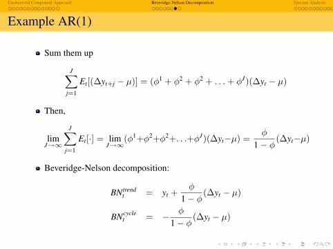
Sum them up

J∑j=1

Et[(∆yt+j − µ)] = (φ1 + φ2 + φ2 + . . .+ φJ)(∆yt − µ)

Then,

limJ→∞

J∑j=1

Et[·] = limJ→∞

(φ1+φ2+φ2+. . .+φJ)(∆yt−µ) =φ

1− φ(∆yt−µ)

Beveridge-Nelson decomposition:

BN trendt = yt +

φ

1− φ(∆yt − µ)

BNcyclet = − φ

1− φ(∆yt − µ)


Remarks

BN decomposition vary: for different forecasting model we havedifferent BN decomposition.E[τt|Ωt] - true trend with unobserved component model.Trend follows random walk in both interpretations. And variability ofthis RW is the same under both interpretations.BN trend estimate of true trend (KF).BN is applicable to any forecasting model: linear and non-linear.BN avoids spurious cycles (unlike HP and Baxter-King).


Time Domain

Wold Form:

Yt = µ+∞∑

j=0

Ψjεt−j, ε ∼ WN

The Yt process can be decomposed into the sum of linearcombination of shocks (errors).It’s time domain because we can see Yt as function of past (in time)realization of shocks.


Frequency Domain

For covariance-stationary process

Yt = µ+∫ π

0α(ω) cos(ωt)dω +

∫ π

0δ(ω) sin(ωt)dω

It’s a weighted average (in continuous time) of periodic cycles (sin andcos).ω determines periods: how frequent the cycles are


Cos

Plot@[email protected] xD, 8x, 0, 2 Pi<, Ticks → 880, Pi, 2 Pi<, 8−1, 1<<D

p 2 p

-1

1

Plot@Cos@2 xD, 8x, 0, 2 Pi<, Ticks → 880, Pi, 2 Pi<, 8−1, 1<<D

p 2 p

-1

1

Plot@Cos@4 xD, 8x, 0, 2 Pi<, Ticks → 880, Pi, 2 Pi<, 8−1, 1<<D

p 2 p

-1

1


Auto-covariance Generating Function

Autocovariance Generating Function,

gy(z) =∞∑

j=−∞γjzj

wherez is a complex scalarj-th autocovariance

γj = E[(Yt − µ)(Yt−j − µ)]

Exist if the sequence of autocovariances γj∞j=−∞ is absolutelysummable

A function of all autocovariances for covariance-stationary process.For a covariance-stationary process it is a finite number.


Population spectrum

Population spectrum

SY(ω) =1

2πgy(e−iω) =

12π

∞∑j=∞

γje−iωj,

ω is a real scalar.Since e−iωj = cos(ωj)− i sin(ωj)

SY(ω) =1

2π

γ0 + 2∞∑

j=1

γj cos(ωj)

as γj = γ−j.SY(ω)⇔ γj’s.We capture how much variation in time sense is due to variability(cycles) at cos and sin at different frequencies.


Spectral Representation Theorem

For a covariance-stationary process

Yt = µ+∫ π

0[α(ω) cos(ωt) + δ(ω) sin(ωt)] dω

for any frequencies < 0 < ω1 < ω2 < . . . < ωn < π∫ ω2

ω1

α(ω)dω uncorrelated with∫ ω4

ω3

α(ω)dω,

and ∫ ω2

ω1

δ(ω)dω uncorrelated with∫ ω4

ω3

δ(ω)dω.

Decomposition of covariance stationary series into orthogonalcomponents due to cycles at different frequencies.


Example: White Noise

Yt ∼ WN

σ2ê2π

pw

SyHwL

Flat spectrum: 2× area = σ2 = var(Yt).This defines white noise processthere is equal weight on cycles for each frequency: variation is dividedequally by cycles with different frequencies.In general, 2·area under spectral density = variance.


Example: AR(1), MA(1)

E.g. MA(1), AR(1), ARMA(1,1)

p

2p

w0

0.1

0.2

0.3

0.4SyHwL

MAH1L, q=0.5

0 p

2p

w0

0.1

0.2

0.3

0.4

0.5

0.6

0.7SyHwL

ARH1L, f=0.5

Low ω corresponds to low frequency and long cycles.The area under the curve depicts how much variability corresponds togiven frequency of fluctuations.Hight is just as important as shape of the SY(ω).


In the short horizon I can’t see as much variability as over the longertime.For AR(1):

var(Yt|Ωt−1) = σ2, var(Yt) =σ2

1− φ2 , varYt > var(Yt|Ωt−1).

Spectrum only for covariance stationary processes.For AR process there is more variation lower frequency than higher.E.g. AR(2):

There are some frequencies that account for a lot of variation in theprocess.Variation in the process is driven by some middle frequencies.Peak in spectral density could be evidence that RBC are indeed cycles.


RandomnessCycles at frequency zero (it’s not a cycle): how much of the movementare due to shocks that never occur cyclically.Spectral density at frequency zero tells about persistence of series(long-run variance).Suppose Xt is log GDP and Yt GDP growth:

Yt = ∆Xt

ThenSY(0) = S∆X(0)

extent to which a shock to ∆X has permanent effect on X and is not justtransitory cycle.If Xt (level) is covariance-stationary then S∆X(0) = 0

no mass at 0 frequency because no permanent movement in it.


Unit Root

If S∆X(0) 6= 0 then Xt is not covariance stationary.For unit root, SX(0) =∞: accumulation of shocks that never dies out.You can calculate sample spectrum.For non-stationary process we will not get∞, as we would forpopulation, but a number (we can see it as downward bias).


Filtering

It is easy to apply filter to data when you think about spectralrepresentation of the process.Example: GDP has important seasonal component (1-4 quarters).The long-run variability might be swamped by the short-term seasonalvariation.The variation in the series might be due to seasonality while we mightbe more interested in relative lower frequencies.Regressing ∆C on ∆Y might produce wacky results as they might bedriven purely by seasonal behavior.


Filtering

Filtering: remove or isolate movements in covariance-stationary seriesat different horizons: e.g. remove seasonality.Filter is set of weights to be applied to different frequencies:

Yt = h(L)Xt, SY(ω) = |h(e−iω)|2SX(ω)

h(L) is a filter.

E.g. h(L) = 1− L12: seasonal filter for monthly data.Note: do not apply spectral analysis to integrated time series processes(not covariance stationary).If filter is applied to non-stationary series and then it’s differenced thefilter is distorted.We may get spurious cycle: cycles in the place where there are nocycles.

Class: Trend-Cycle Decomposition - Jacek Suda · Unobserved Component Approach Beveridge-Nelson Decomposition Spectral Analysis Beveridge-Nelson Decomposition BN trend is the long-run

Documents