Clarke’s and Park’s Transformations BPRA047, BPRA048

Welcome message from author
This document is posted to help you gain knowledge. Please leave a comment to let me know what you think about it! Share it to your friends and learn new things together.
Transcript
Clarke’s and Park’s Transformations
BPRA047, BPRA048
2008-9-28SUN Dan
College of Electrical Engineering, Zhejiang University 2
Content
1 Introduction2 Clarke’s Transformation3 Park’s Transformation4 Transformations Between Reference Frames5 Field Oriented Control (FOC) Transformations6 Implementing Clarke’s and Park’s Transformations7 Conclusion8 Reading Materials
2008-9-28SUN Dan
College of Electrical Engineering, Zhejiang University 3
Introduction
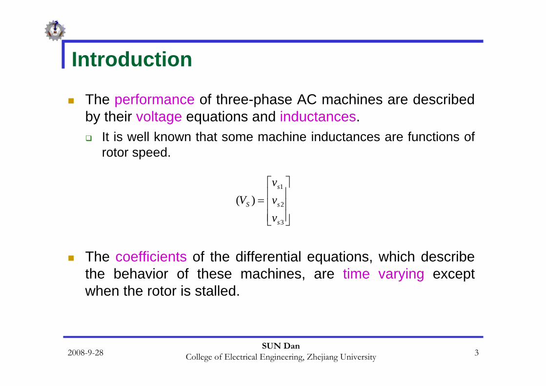
The performance of three-phase AC machines are described by their voltage equations and inductances.
It is well known that some machine inductances are functions of rotor speed.
The coefficients of the differential equations, which describe the behavior of these machines, are time varying except when the rotor is stalled.
⎥⎥⎥
⎦
⎤
⎢⎢⎢
⎣
⎡=
3
2
1
)(
s
s
s
S
vvv
V
2008-9-28SUN Dan
College of Electrical Engineering, Zhejiang University 4
Introduction
A change of variables is often used to reduce the complexity of these differential equations.
In this chapter, the well-known Clarke and Parktransformations are introduced, modeled, and implemented on the LF2407 DSP.
Using these transformations, many properties of electric machines can be studied without complexities in the voltage equations.
2008-9-28SUN Dan
College of Electrical Engineering, Zhejiang University 5
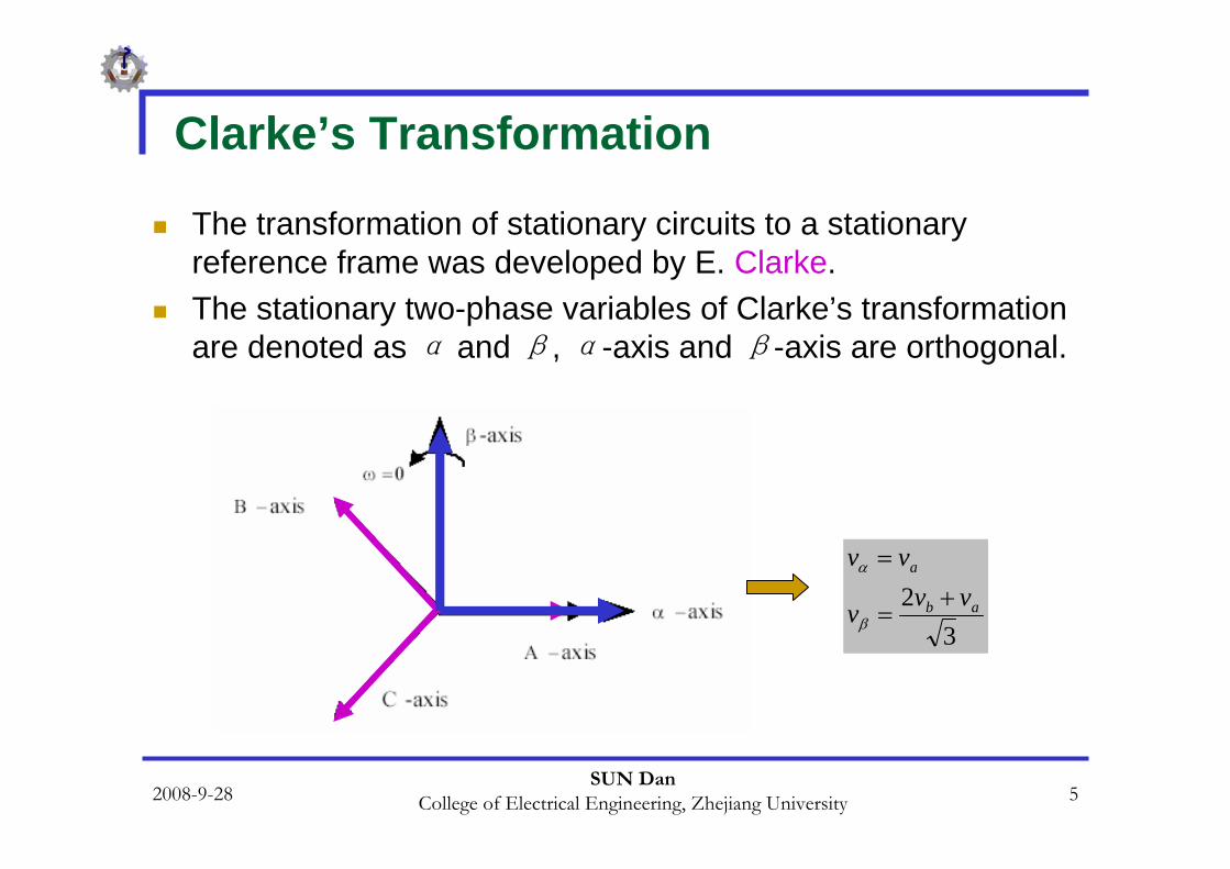
Clarke’s Transformation
The transformation of stationary circuits to a stationary reference frame was developed by E. Clarke.The stationary two-phase variables of Clarke’s transformation are denoted as α and β, α-axis and β-axis are orthogonal.
32 ab
a
vvv
vv+
=
=
β
α
2008-9-28SUN Dan
College of Electrical Engineering, Zhejiang University 6
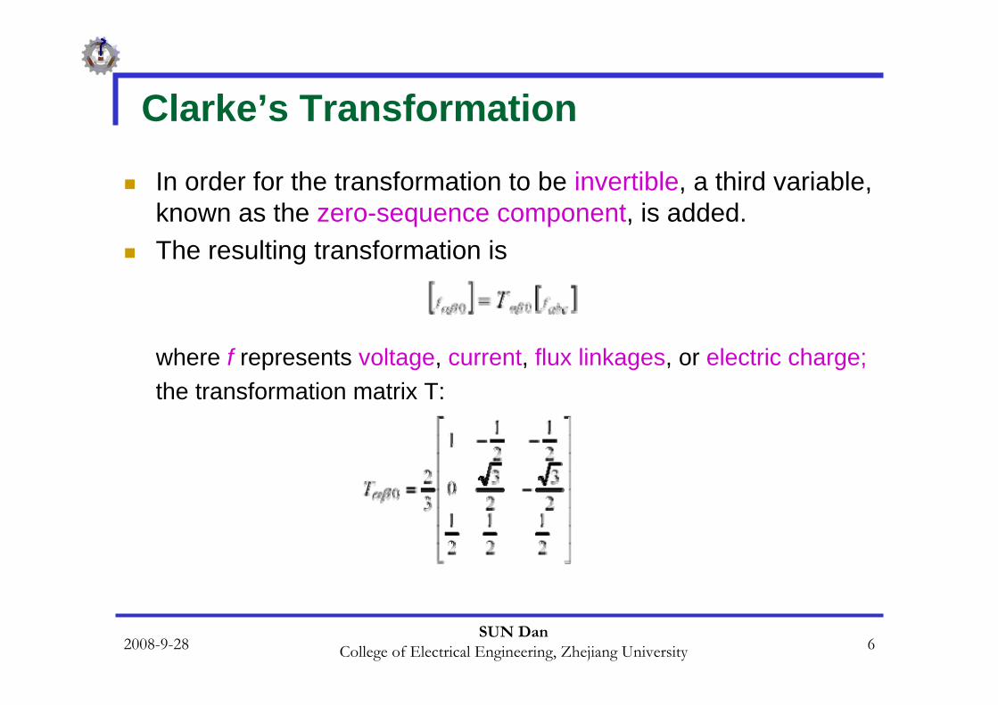
Clarke’s Transformation
In order for the transformation to be invertible, a third variable, known as the zero-sequence component, is added. The resulting transformation is
where f represents voltage, current, flux linkages, or electric charge;the transformation matrix T:
2008-9-28SUN Dan
College of Electrical Engineering, Zhejiang University 7
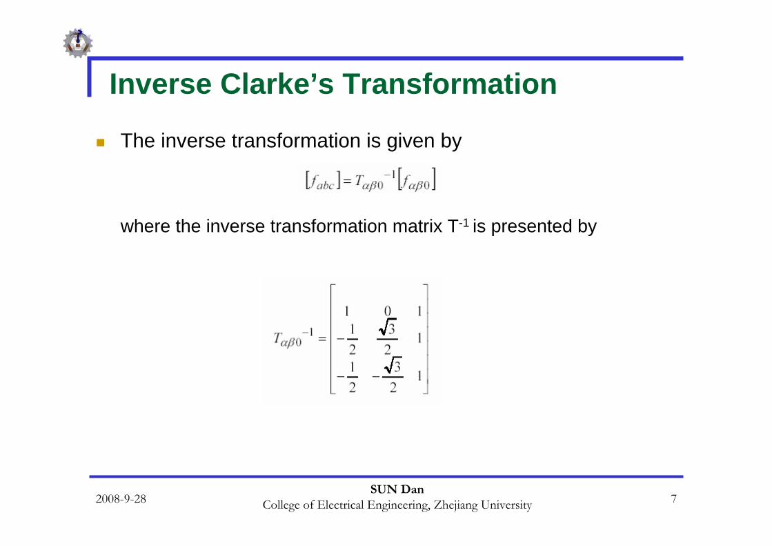
Inverse Clarke’s Transformation
The inverse transformation is given by
where the inverse transformation matrix T-1 is presented by
2008-9-28SUN Dan
College of Electrical Engineering, Zhejiang University 8
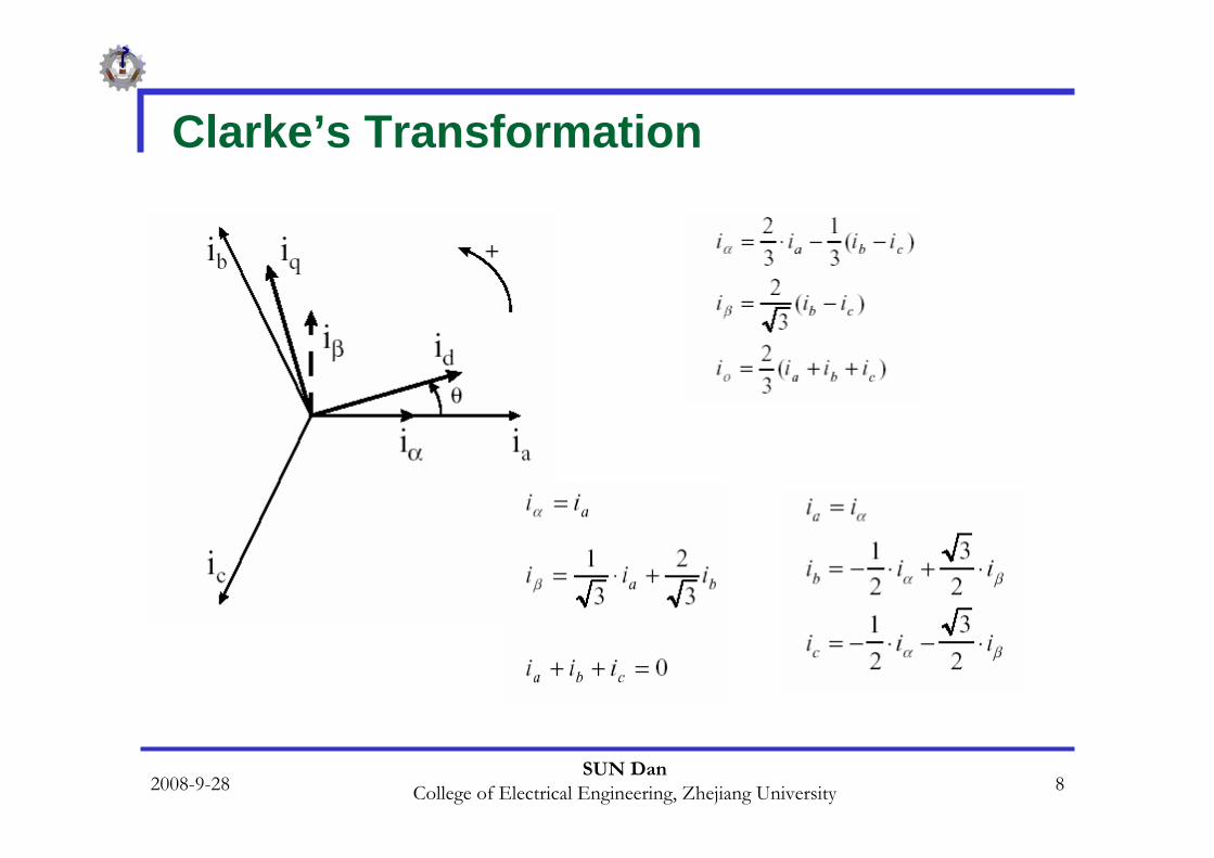
Clarke’s Transformation
2008-9-28SUN Dan
College of Electrical Engineering, Zhejiang University 9
Park’s Transformation
In the late 1920s, R.H. Park introduced a new approach to electric machine analysis. He formulated a change of variables associated with fictitious windings rotating with the rotor. He referred the stator and rotor variables to a reference frame fixedon the rotor. From the rotor point of view, all the variables can be observed as constant values.
Park’s transformation, a revolution in machine analysis, has the unique property of eliminating all time varying inductances from the voltage equations of three-phase ac machines due to the rotor spinning.
2008-9-28SUN Dan
College of Electrical Engineering, Zhejiang University 10
Park’s Transformation
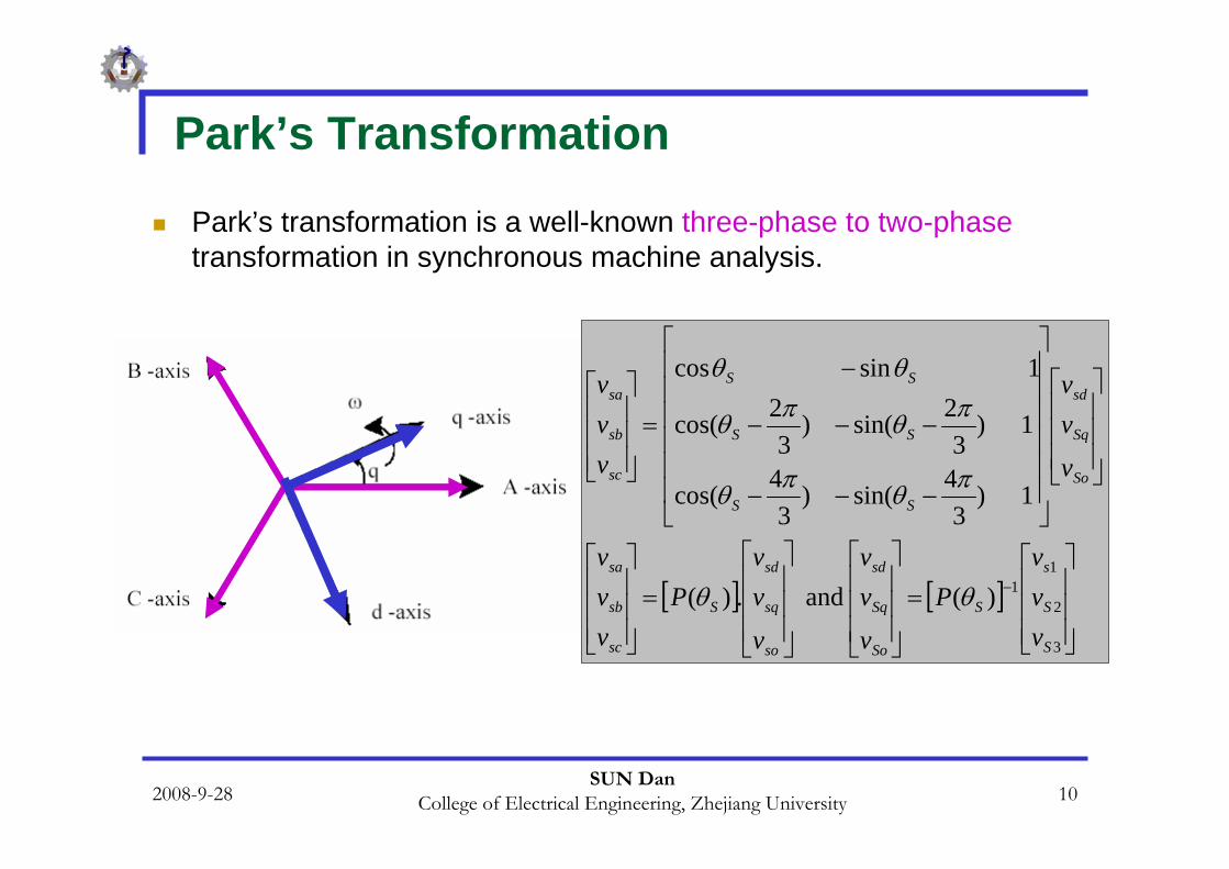
Park’s transformation is a well-known three-phase to two-phasetransformation in synchronous machine analysis.
[ ] [ ]⎥⎥⎥
⎦
⎤
⎢⎢⎢
⎣
⎡=
⎥⎥⎥
⎦
⎤
⎢⎢⎢
⎣
⎡
⎥⎥⎥
⎦
⎤
⎢⎢⎢
⎣
⎡
=⎥⎥⎥
⎦
⎤
⎢⎢⎢
⎣
⎡
⎥⎥⎥
⎦
⎤
⎢⎢⎢
⎣
⎡
⎥⎥⎥⎥⎥⎥
⎦
⎤
⎢⎢⎢⎢⎢⎢
⎣
⎡
−−−
−−−
−
=⎥⎥⎥
⎦
⎤
⎢⎢⎢
⎣
⎡
−
3
2
11)( and .)(
1 )3
4sin( )3
4cos(
1 )3
2sin( )3
2cos(
1 sin cos
S
S
s
S
So
Sq
sd
so
sq
sd
S
sc
sb
sa
So
Sq
sd
SS
SS
SS
sc
sb
sa
vvv
P
v
vv
v
vv
Pvvv
v
vv
vvv
θθ
πθπθ
πθπθ
θθ
2008-9-28SUN Dan
College of Electrical Engineering, Zhejiang University 11
Park’s Transformation
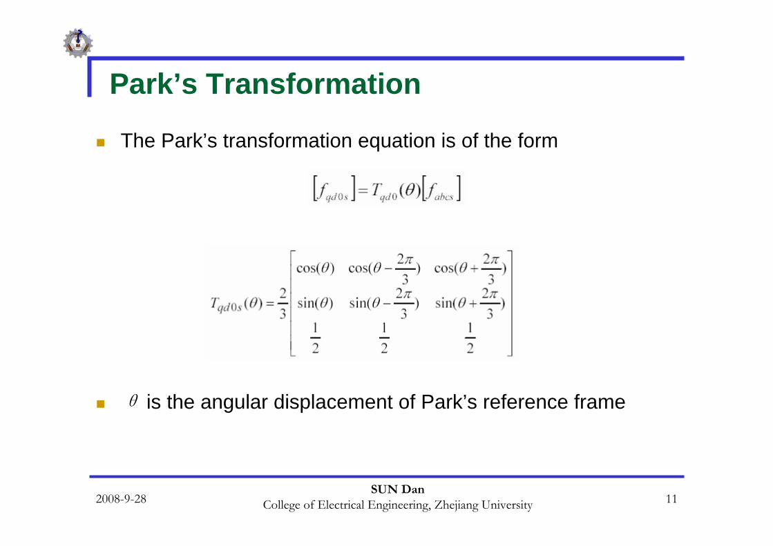
The Park’s transformation equation is of the form
θ is the angular displacement of Park’s reference frame
2008-9-28SUN Dan
College of Electrical Engineering, Zhejiang University 12
Inverse Park’s Transformation
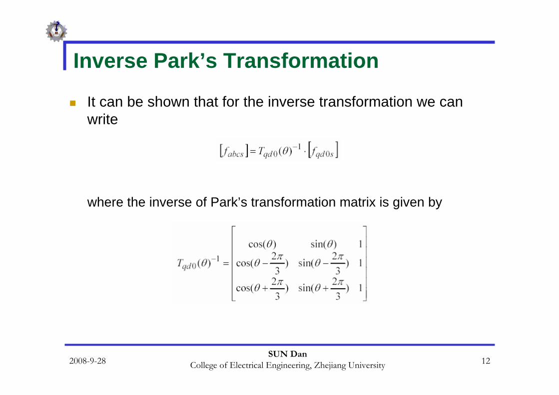
It can be shown that for the inverse transformation we can write
where the inverse of Park’s transformation matrix is given by
2008-9-28SUN Dan
College of Electrical Engineering, Zhejiang University 13
Park’s Transformation
The angular displacement θ must be continuous, but the angular velocity associated with the change of variables is unspecified. The frame of reference may rotate at any constant, varying angular velocity, or it may remain stationary. The angular velocity of the transformation can be chosen arbitrarily to best fit the system equation solution or to satisfy the system constraints.
The change of variables may be applied to variables of any waveform and time sequence;
however, we will find that the transformation given above is particularly appropriate for an a-b-c sequence.
2008-9-28SUN Dan
College of Electrical Engineering, Zhejiang University 14
Park’s Transformation
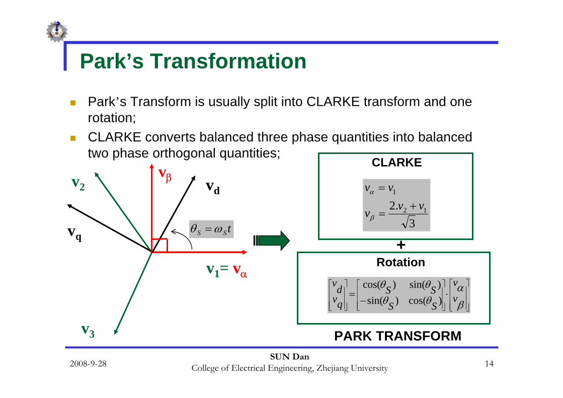
Park’s Transform is usually split into CLARKE transform and one rotation;CLARKE converts balanced three phase quantities into balanced two phase orthogonal quantities;
tSS ωθ =
v1= vα
v3
v2vβ vd
vq3
.2 12
1
vvv
vv+
=
=
β
α
⎥⎥⎥
⎦
⎤
⎢⎢⎢
⎣
⎡
⎥⎥⎥
⎦
⎤
⎢⎢⎢
⎣
⎡
⎥⎥⎥
⎦
⎤
⎢⎢⎢
⎣
⎡⋅
−=
βα
θθθθ
vv
SSSS
qvdv
)cos()sin()sin()cos(
CLARKE
+Rotation
PARK TRANSFORM
2008-9-28SUN Dan
College of Electrical Engineering, Zhejiang University 15
Park’s Transformation
2008-9-28SUN Dan
College of Electrical Engineering, Zhejiang University 16
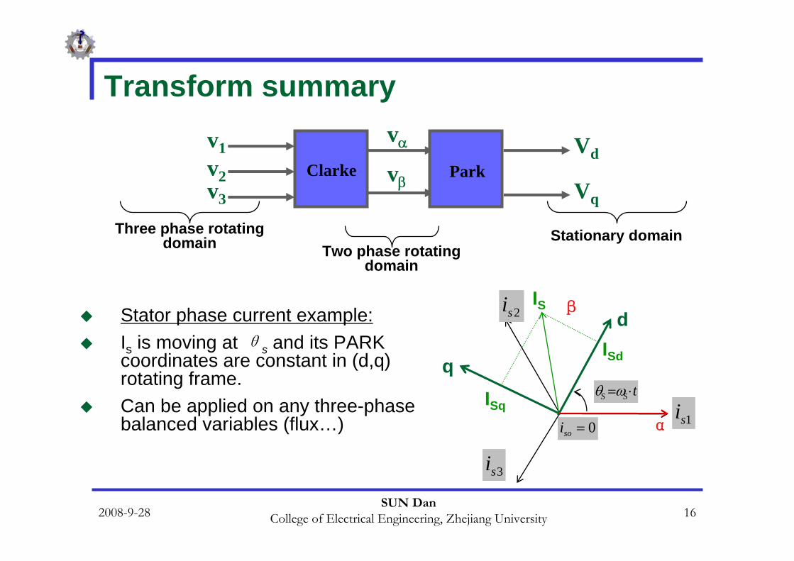
Transform summary
Three phase rotating domain Two phase rotating
domain
Stationary domain
Stator phase current example:Is is moving at θs and its PARK coordinates are constant in (d,q) rotating frame.Can be applied on any three-phase balanced variables (flux…) 1si
3si
2si
0=soi
tSS ⋅=ωθ
IS
ISd
ISq
d
q
α
β
Clarke
v1v2v3
vαvβ Park
Vd
Vq
2008-9-28SUN Dan
College of Electrical Engineering, Zhejiang University 17
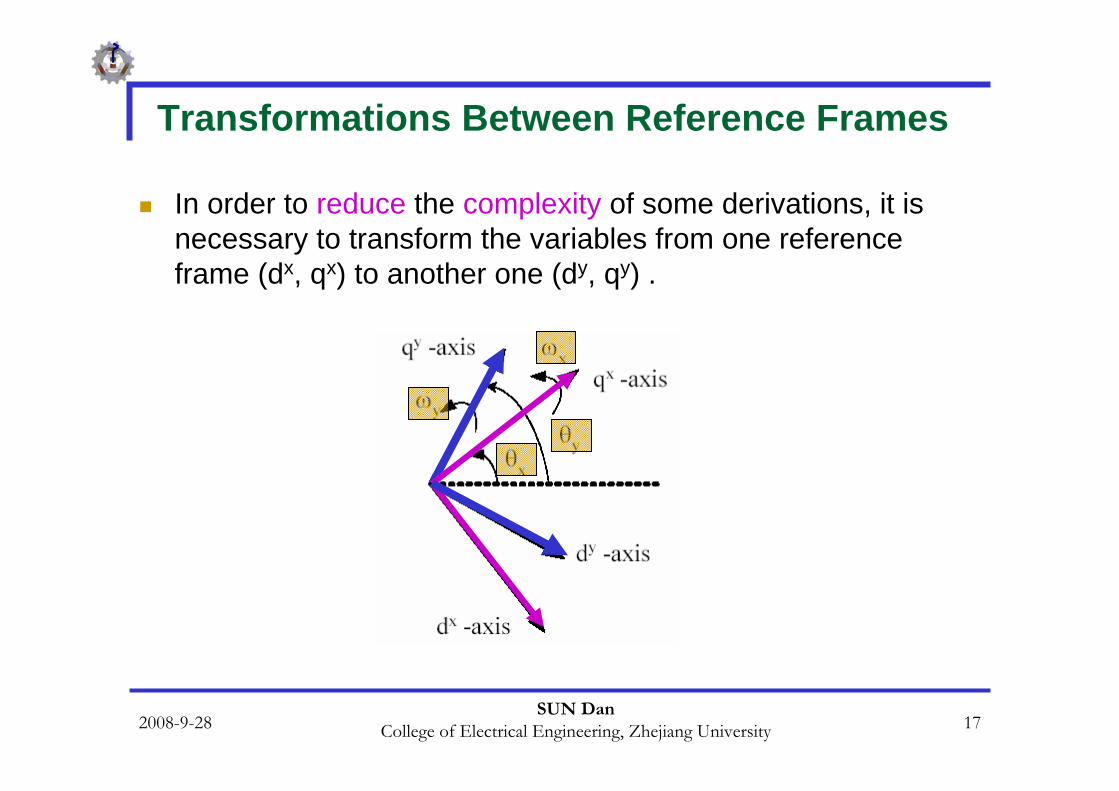
Transformations Between Reference Frames
In order to reduce the complexity of some derivations, it is necessary to transform the variables from one reference frame (dx, qx) to another one (dy, qy) .
2008-9-28SUN Dan
College of Electrical Engineering, Zhejiang University 18
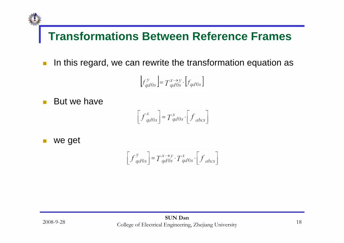
Transformations Between Reference Frames
In this regard, we can rewrite the transformation equation as
But we have
we get
2008-9-28SUN Dan
College of Electrical Engineering, Zhejiang University 19
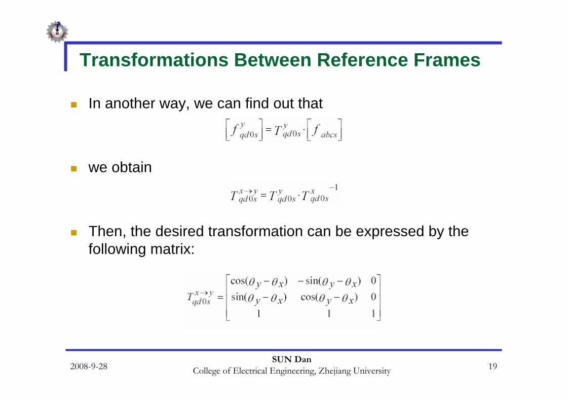
Transformations Between Reference Frames
In another way, we can find out that
we obtain
Then, the desired transformation can be expressed by the following matrix:
2008-9-28SUN Dan
College of Electrical Engineering, Zhejiang University 20
Field Oriented Control (FOC) Transformations
In the case of FOC of electric machines, control methods are performed in a two-phase reference frame fixed to the rotor (qr-dr) or fixed to the excitation reference frame (qe-de).
We want to transform all the variables from the three-phase a-b-c system to the two-phase stationary reference frame and then retransform these variables from the stationary reference frame to a rotary reference frame with arbitrary angular velocity of ω.
2008-9-28SUN Dan
College of Electrical Engineering, Zhejiang University 21
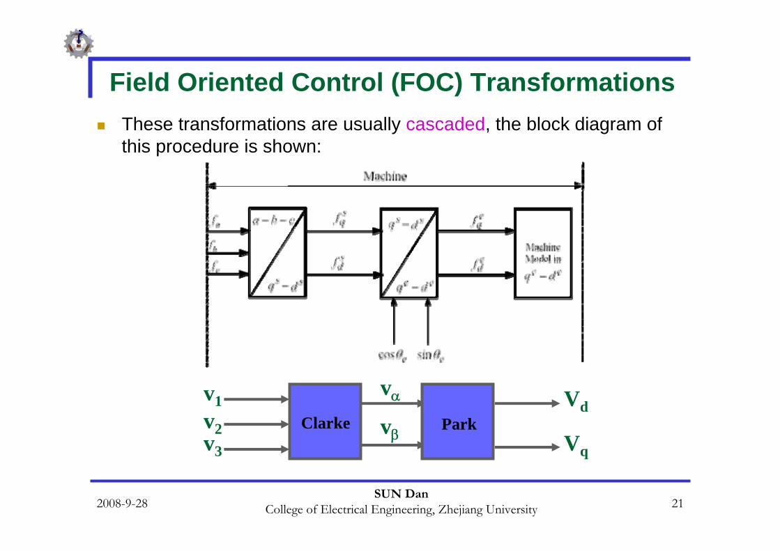
Field Oriented Control (FOC) TransformationsThese transformations are usually cascaded, the block diagram of this procedure is shown:
Clarke
v1v2v3
vαvβ Park
Vd
Vq
2008-9-28SUN Dan
College of Electrical Engineering, Zhejiang University 22
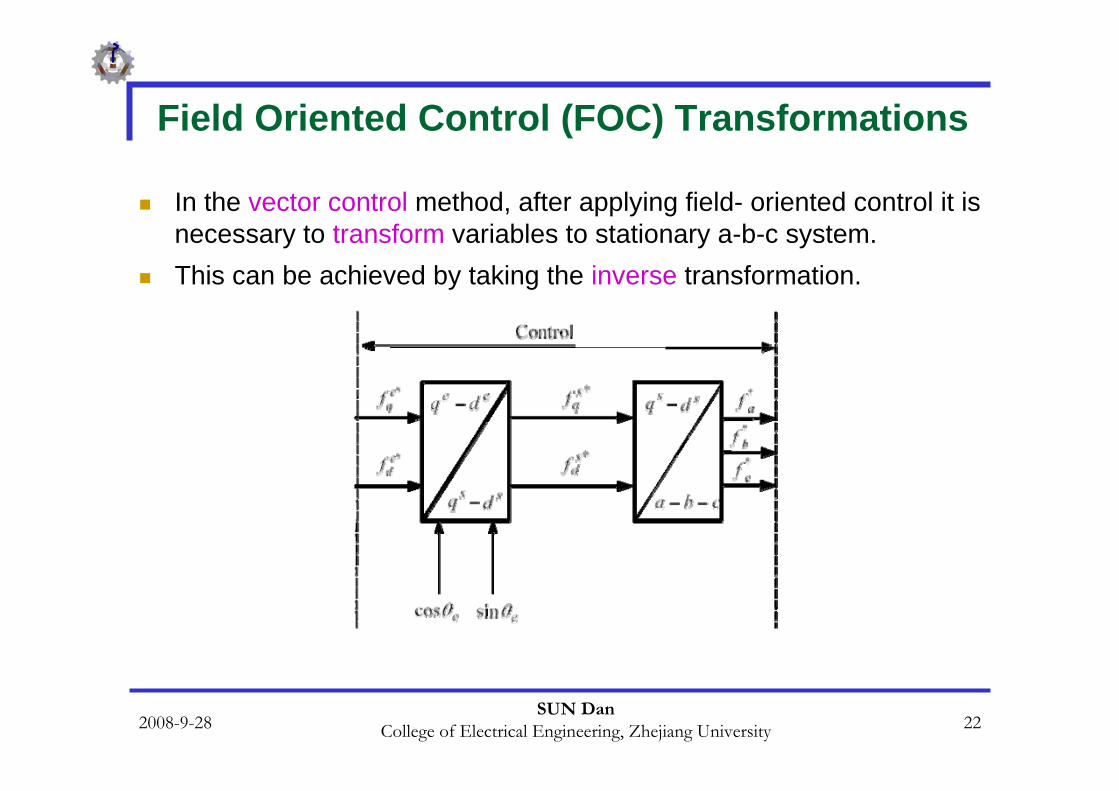
Field Oriented Control (FOC) Transformations
In the vector control method, after applying field- oriented control it is necessary to transform variables to stationary a-b-c system. This can be achieved by taking the inverse transformation.
2008-9-28SUN Dan
College of Electrical Engineering, Zhejiang University 23
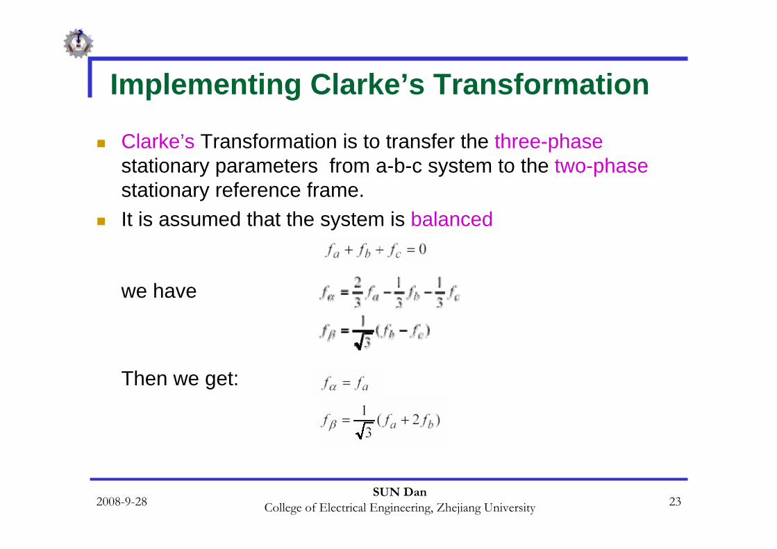
Implementing Clarke’s Transformation
Clarke’s Transformation is to transfer the three-phasestationary parameters from a-b-c system to the two-phasestationary reference frame. It is assumed that the system is balanced
we have
Then we get:
2008-9-28SUN Dan
College of Electrical Engineering, Zhejiang University 24
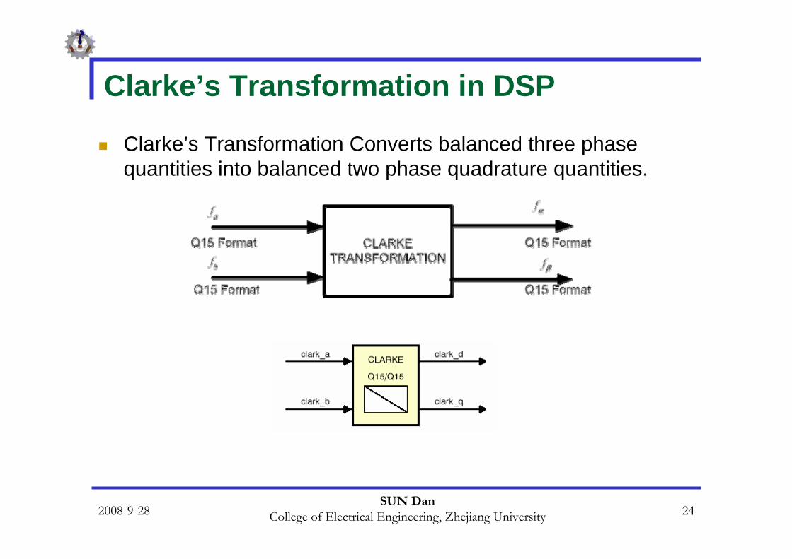
Clarke’s Transformation in DSP
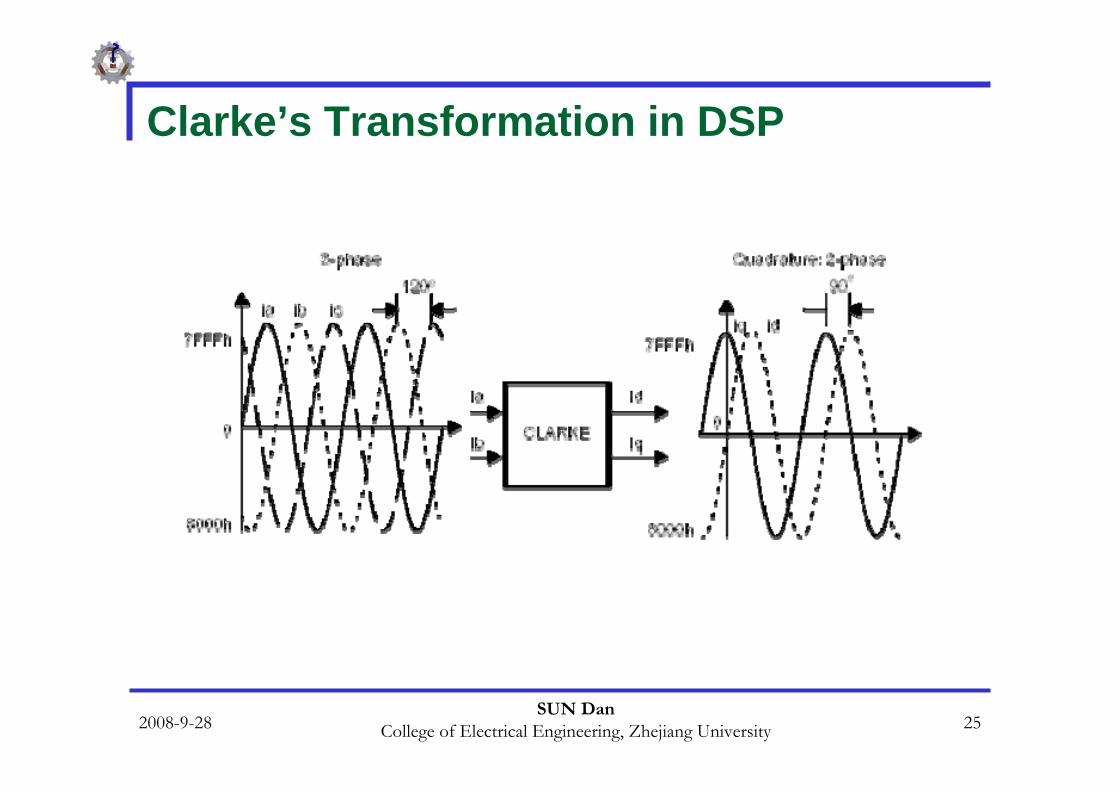
Clarke’s Transformation Converts balanced three phase quantities into balanced two phase quadrature quantities.
2008-9-28SUN Dan
College of Electrical Engineering, Zhejiang University 25
Clarke’s Transformation in DSP
2008-9-28SUN Dan
College of Electrical Engineering, Zhejiang University 26
Clarke’s Transformation in DSP
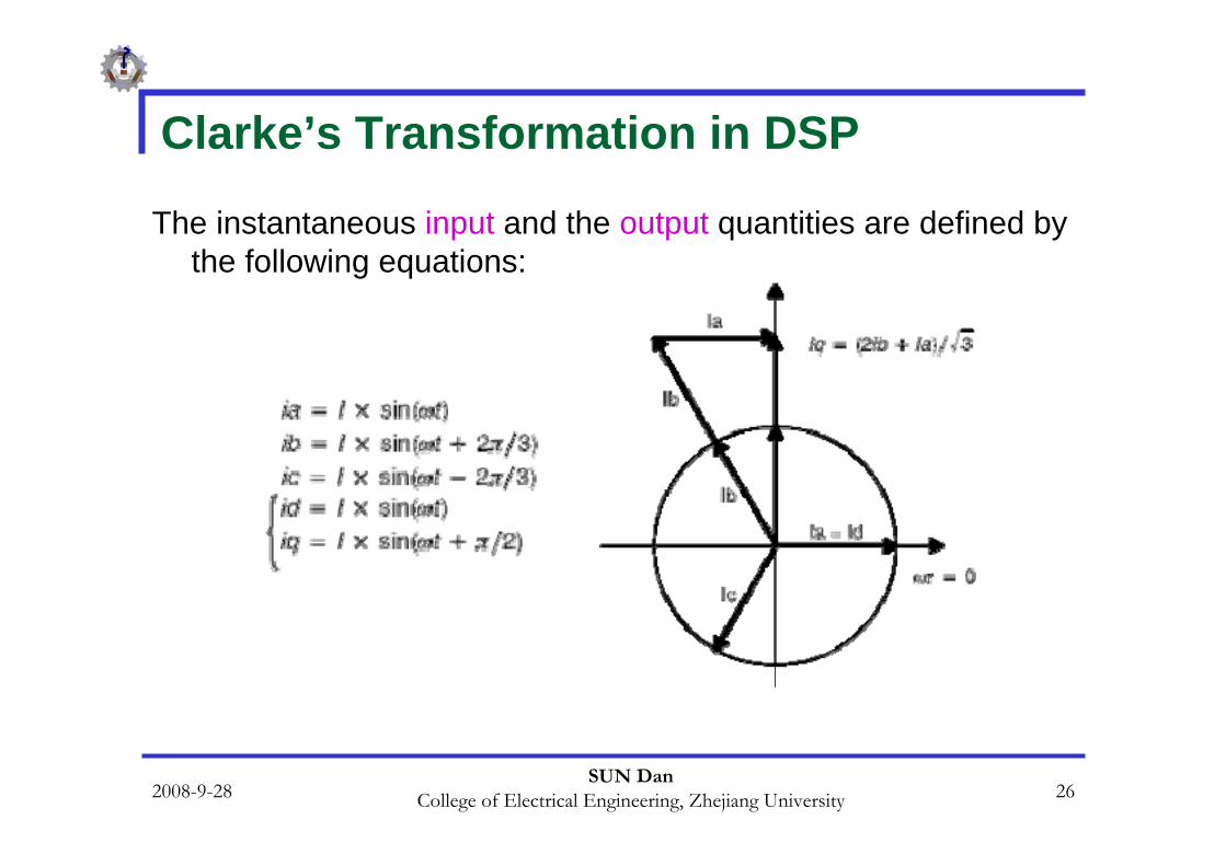
The instantaneous input and the output quantities are defined by the following equations:
2008-9-28SUN Dan
College of Electrical Engineering, Zhejiang University 27
Clarke’s Transformation in DSP
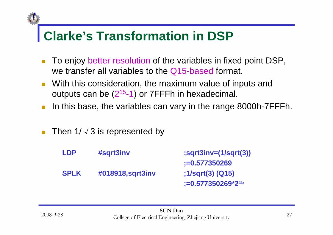
To enjoy better resolution of the variables in fixed point DSP, we transfer all variables to the Q15-based format. With this consideration, the maximum value of inputs and outputs can be (215-1) or 7FFFh in hexadecimal. In this base, the variables can vary in the range 8000h-7FFFh.
Then 1/√3 is represented by
LDP #sqrt3inv ;sqrt3inv=(1/sqrt(3)) ;=0.577350269
SPLK #018918,sqrt3inv ;1/sqrt(3) (Q15) ;=0.577350269*215
2008-9-28SUN Dan
College of Electrical Engineering, Zhejiang University 28
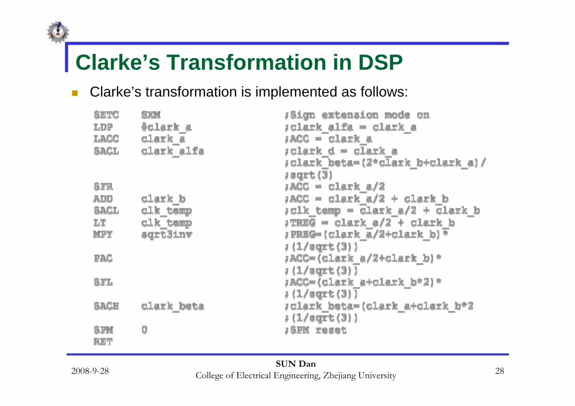
Clarke’s Transformation in DSPClarke’s transformation is implemented as follows:
2008-9-28SUN Dan
College of Electrical Engineering, Zhejiang University 29
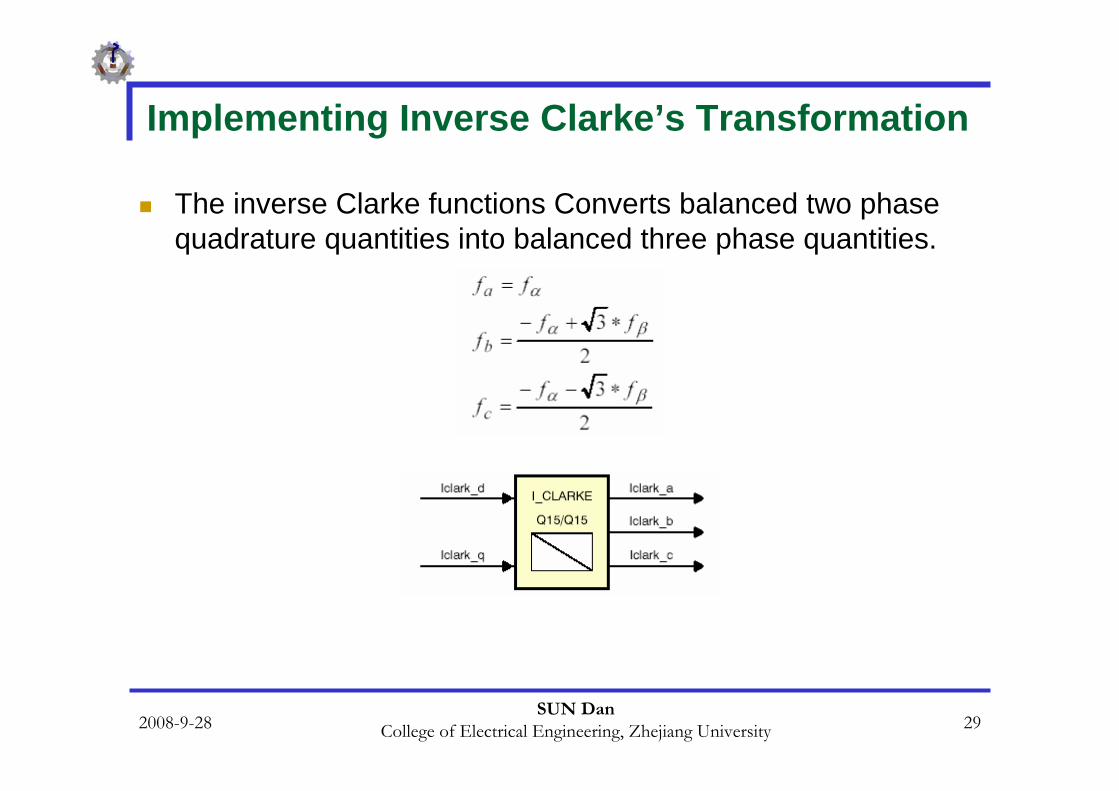
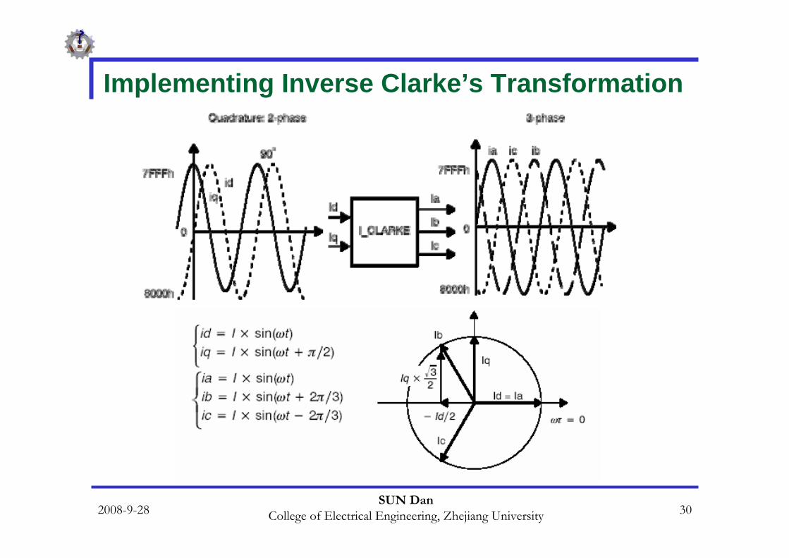
Implementing Inverse Clarke’s Transformation
The inverse Clarke functions Converts balanced two phase quadrature quantities into balanced three phase quantities.
2008-9-28SUN Dan
College of Electrical Engineering, Zhejiang University 30
Implementing Inverse Clarke’s Transformation
2008-9-28SUN Dan
College of Electrical Engineering, Zhejiang University 31
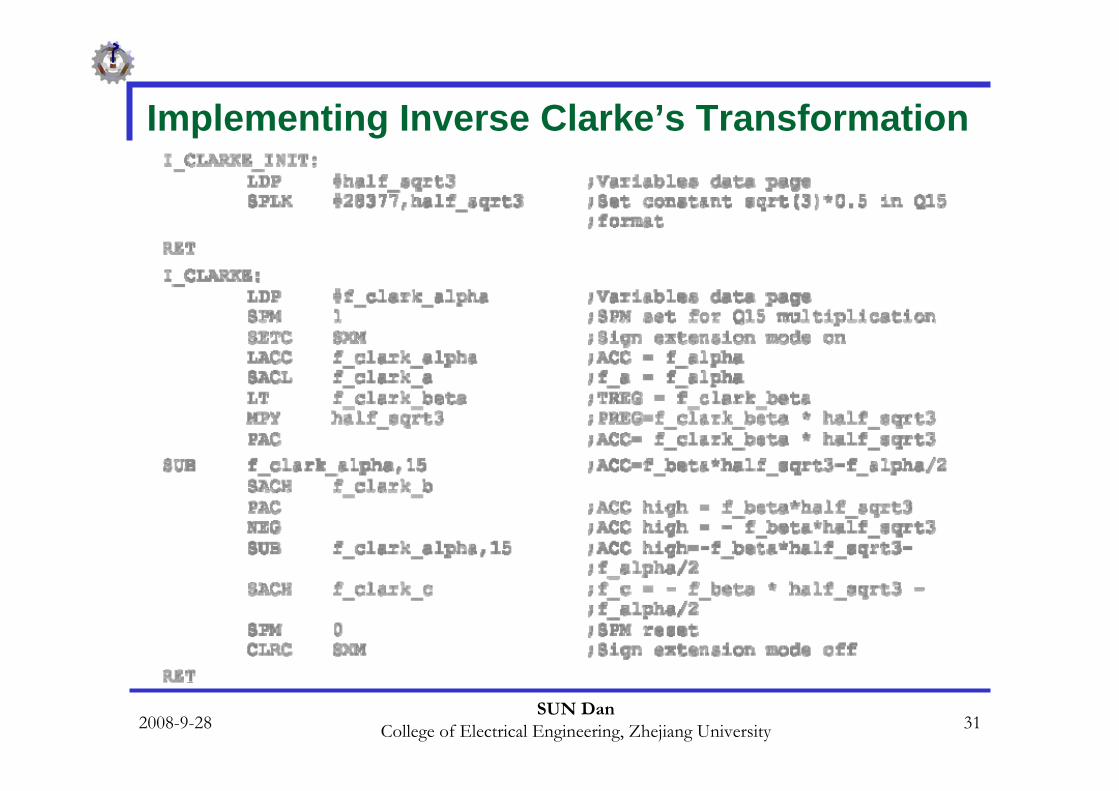
Implementing Inverse Clarke’s Transformation
2008-9-28SUN Dan
College of Electrical Engineering, Zhejiang University 32
Calculation of Sine/Cosine
To implement the Park and the inverse Park transforms, the sine and cosine functions need to be implemented.
This method realizes the sine/cosine functions with a look-uptable of 256 values for 360°of sine and cosine functions.
The method includes linear interpolation with a fixed step table to provide a minimum harmonic distortion.
This table is loaded in program memory.
The sine value is presented in Q15 format with the range of -1<value<1.

2008-9-28SUN Dan
College of Electrical Engineering, Zhejiang University 33
Calculation of Sine/Cosine
The first few rows of the look-up sine table are presented as follows:
;SINVALUE ; Index Angle Sin(Angle)---------------- -------- -------- ------------SINTAB_360 .word 0 ; 0 0 0.0000 .word 804 ; 1 1.41 0.0245 .word 1608 ; 2 2.81 0.0491 .word 2410 ; 3 4.22 0.0736 .word 3212 ; 4 5.63 0.0980
2008-9-28SUN Dan
College of Electrical Engineering, Zhejiang University 34
Calculation of Sine/Cosine
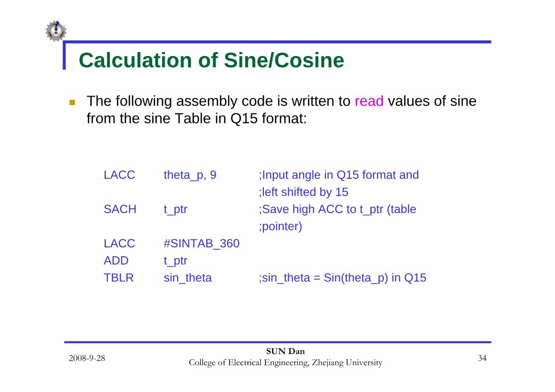
The following assembly code is written to read values of sine from the sine Table in Q15 format:
LACC theta_p, 9 ;Input angle in Q15 format and ;left shifted by 15
SACH t_ptr ;Save high ACC to t_ptr (table ;pointer)
LACC #SINTAB_360 ADD t_ptrTBLR sin_theta ;sin_theta = Sin(theta_p) in Q15
2008-9-28SUN Dan
College of Electrical Engineering, Zhejiang University 35
Calculation of Sine/Cosine
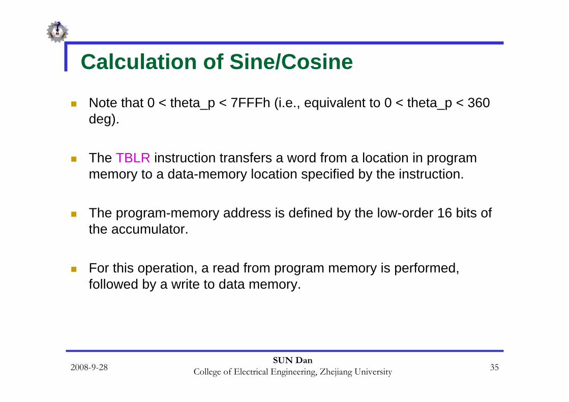
Note that 0 < theta_p < 7FFFh (i.e., equivalent to 0 < theta_p < 360 deg).
The TBLR instruction transfers a word from a location in program memory to a data-memory location specified by the instruction.
The program-memory address is defined by the low-order 16 bits of the accumulator.
For this operation, a read from program memory is performed, followed by a write to data memory.
2008-9-28SUN Dan
College of Electrical Engineering, Zhejiang University 36
Calculation of Sine/Cosine
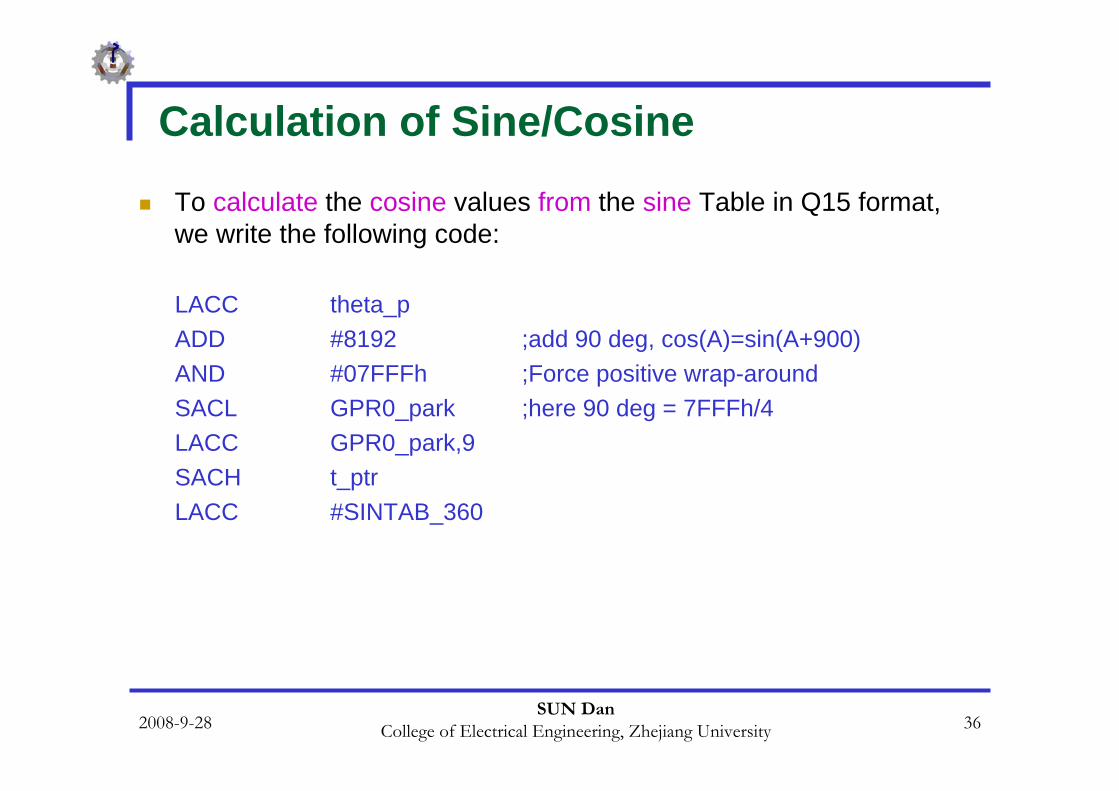
To calculate the cosine values from the sine Table in Q15 format, we write the following code:
LACC theta_pADD #8192 ;add 90 deg, cos(A)=sin(A+900) AND #07FFFh ;Force positive wrap-around SACL GPR0_park ;here 90 deg = 7FFFh/4 LACC GPR0_park,9 SACH t_ptrLACC #SINTAB_360
2008-9-28SUN Dan
College of Electrical Engineering, Zhejiang University 37
Implementation of Park’s Transformation
With field-oriented control of motors, it is necessary to transform variables,
from a-b-c system to two-phase stationary reference frame, qs-ds, and from two-phase stationary reference frame qs-ds to arbitrary rotating reference frame with angular velocity of ω (q-d reference frame).
The first transformation is dual to Clarke’s transformation but the qs axis is in the direction of α-axis, and ds axis is in negative direction of β-axis.
2008-9-28SUN Dan
College of Electrical Engineering, Zhejiang University 38
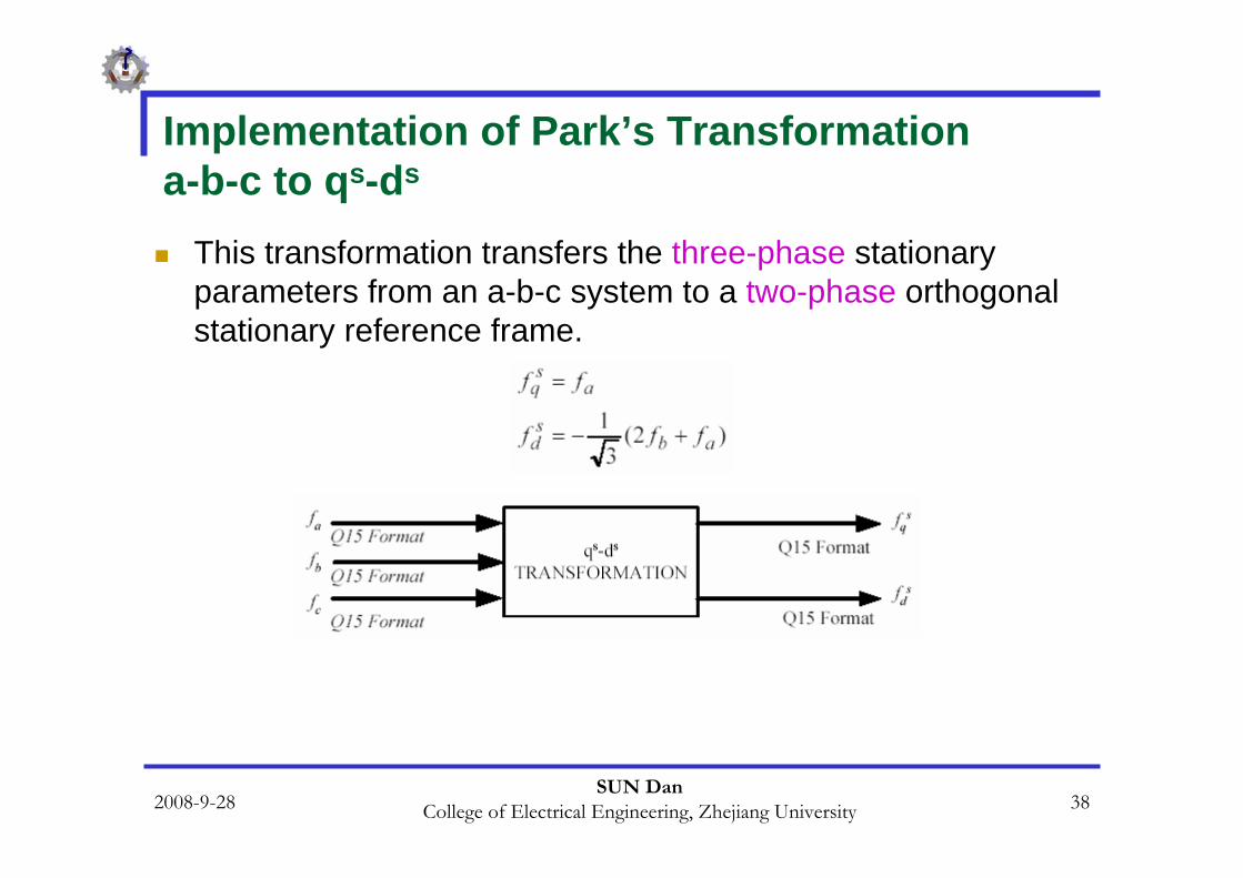
Implementation of Park’s Transformationa-b-c to qs-ds
This transformation transfers the three-phase stationary parameters from an a-b-c system to a two-phase orthogonal stationary reference frame.
2008-9-28SUN Dan
College of Electrical Engineering, Zhejiang University 39
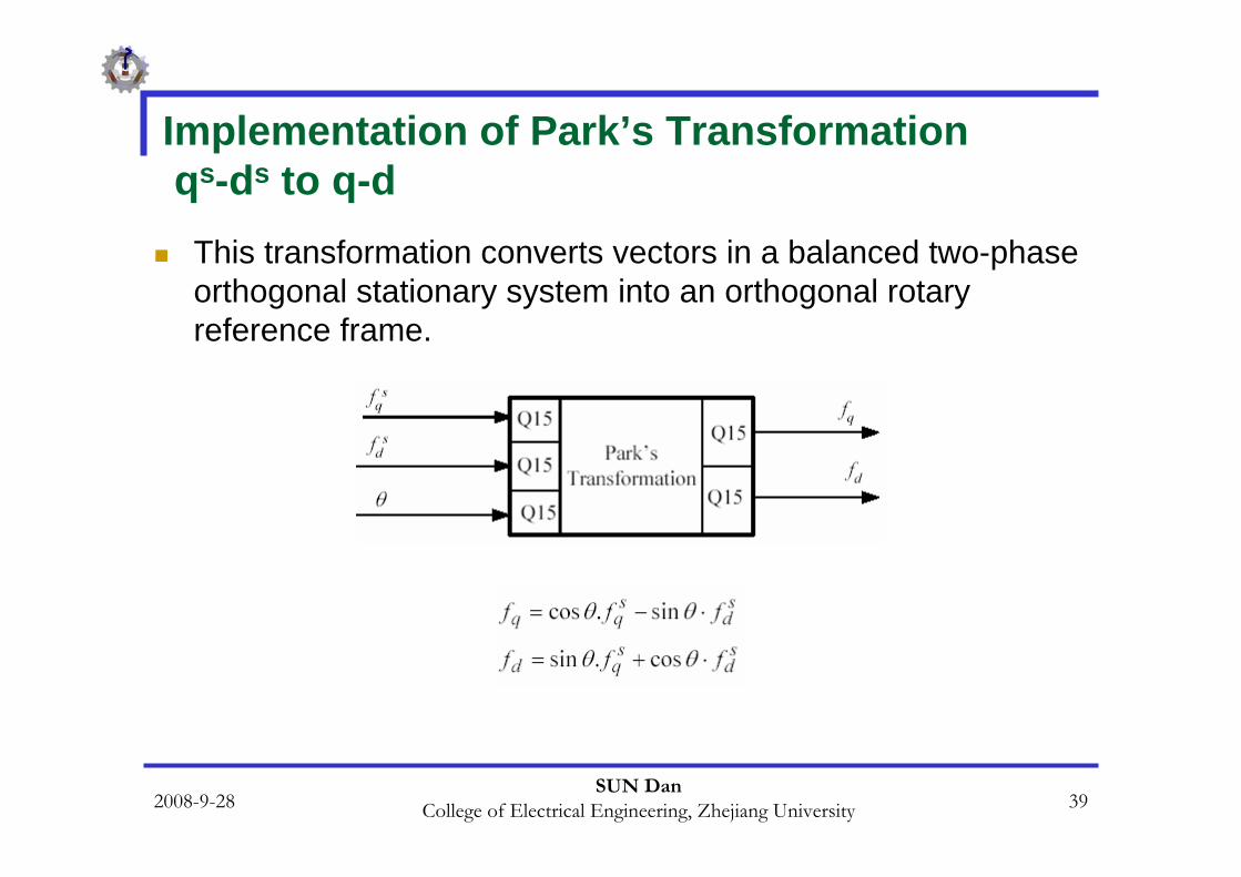
Implementation of Park’s Transformationqs-ds to q-d
This transformation converts vectors in a balanced two-phase orthogonal stationary system into an orthogonal rotary reference frame.
2008-9-28SUN Dan
College of Electrical Engineering, Zhejiang University 40
Implementation of Park’s Transformationqs-ds to q-d
In this transformation, it is necessary to calculate sinθ and cosθ, where the method to calculate them was presented in a previous section.
All the input and outputs are in the Q15 format and in the range of 8000h-7FFFh
2008-9-28SUN Dan
College of Electrical Engineering, Zhejiang University 41
Implementation of Park’s Transformationqs-ds to q-d
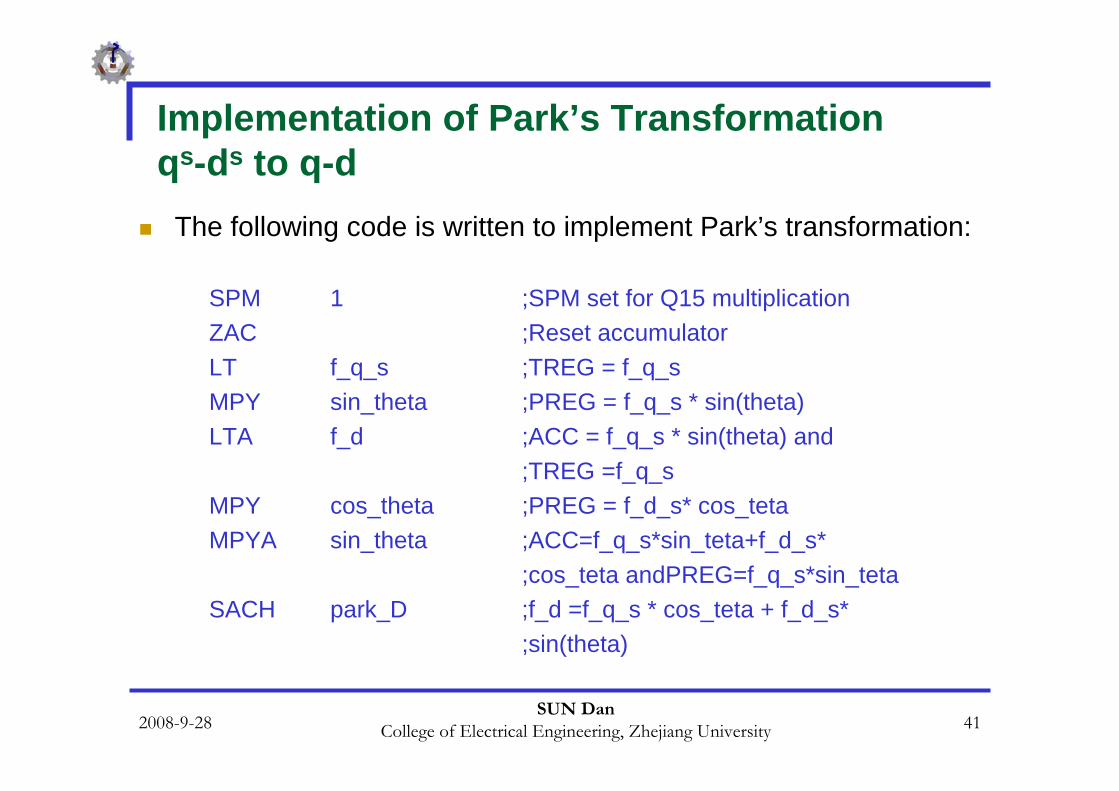
The following code is written to implement Park’s transformation:
SPM 1 ;SPM set for Q15 multiplication ZAC ;Reset accumulator LT f_q_s ;TREG = f_q_sMPY sin_theta ;PREG = f_q_s * sin(theta) LTA f_d ;ACC = f_q_s * sin(theta) and
;TREG =f_q_sMPY cos_theta ;PREG = f_d_s* cos_tetaMPYA sin_theta ;ACC=f_q_s*sin_teta+f_d_s*
;cos_teta andPREG=f_q_s*sin_tetaSACH park_D ;f_d =f_q_s * cos_teta + f_d_s*
;sin(theta)
2008-9-28SUN Dan
College of Electrical Engineering, Zhejiang University 42
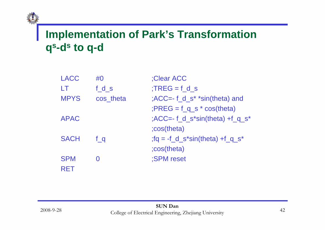
Implementation of Park’s Transformationqs-ds to q-d
LACC #0 ;Clear ACC LT f_d_s ;TREG = f_d_sMPYS cos_theta ;ACC=- f_d_s* *sin(theta) and
;PREG = f_q_s * cos(theta) APAC ;ACC=- f_d_s*sin(theta) +f_q_s*
;cos(theta) SACH f_q ;fq = -f_d_s*sin(theta) +f_q_s*
;cos(theta) SPM 0 ;SPM reset RET
2008-9-28SUN Dan
College of Electrical Engineering, Zhejiang University 43
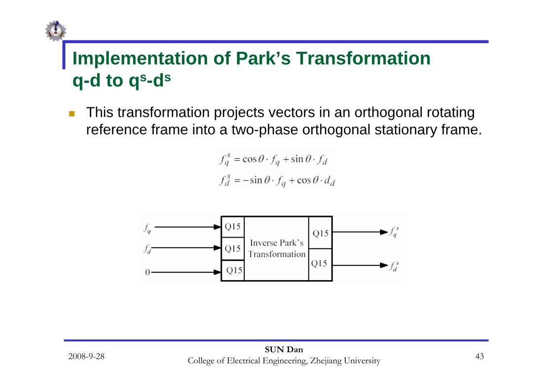
Implementation of Park’s Transformationq-d to qs-ds
This transformation projects vectors in an orthogonal rotating reference frame into a two-phase orthogonal stationary frame.
2008-9-28SUN Dan
College of Electrical Engineering, Zhejiang University 44
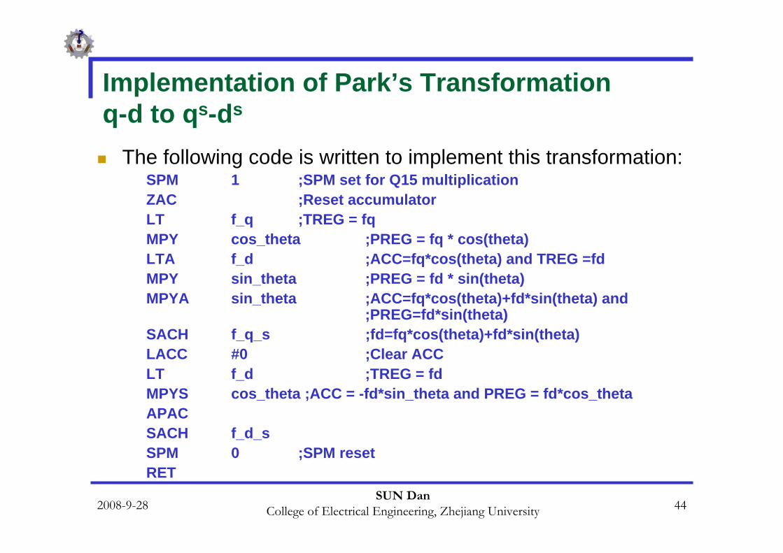
Implementation of Park’s Transformationq-d to qs-ds
The following code is written to implement this transformation: SPM 1 ;SPM set for Q15 multiplication ZAC ;Reset accumulator LT f_q ;TREG = fqMPY cos_theta ;PREG = fq * cos(theta) LTA f_d ;ACC=fq*cos(theta) and TREG =fdMPY sin_theta ;PREG = fd * sin(theta) MPYA sin_theta ;ACC=fq*cos(theta)+fd*sin(theta) and
;PREG=fd*sin(theta) SACH f_q_s ;fd=fq*cos(theta)+fd*sin(theta) LACC #0 ;Clear ACC LT f_d ;TREG = fdMPYS cos_theta ;ACC = -fd*sin_theta and PREG = fd*cos_thetaAPAC SACH f_d_sSPM 0 ;SPM reset RET
2008-9-28SUN Dan
College of Electrical Engineering, Zhejiang University 45
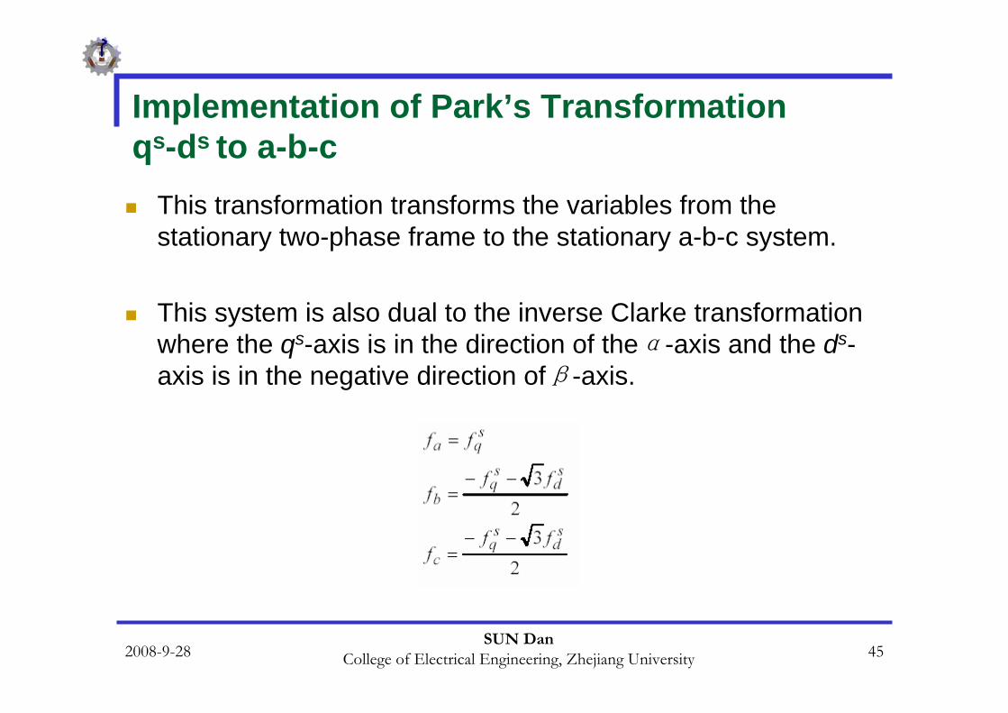
Implementation of Park’s Transformationqs-ds to a-b-c
This transformation transforms the variables from the stationary two-phase frame to the stationary a-b-c system.
This system is also dual to the inverse Clarke transformation where the qs-axis is in the direction of theα-axis and the ds-axis is in the negative direction ofβ-axis.
2008-9-28SUN Dan
College of Electrical Engineering, Zhejiang University 46
Conclusion
With FOC of synchronous and induction machines, it is desirable to reduce the complexity of the electric machine voltage equations.
The transformation of machine variables to an orthogonal reference frame is beneficial for this purpose.
Park’s and Clarke’s transformations, two revolutions in the field of electrical machines, were studied in depth in this chapter.
These transformations and their inverses were implemented on the fixed point LF2407 DSP.
2008-9-28SUN Dan
College of Electrical Engineering, Zhejiang University 47
Reading materials
Bpra047 - Sine, Cosine on the TMS320C2xx
Bpra048 - Clarke & Park Transforms on the TMS320C2xx
Spru485a - Digital Motor Control Software LibraryCLARKE,PARK,I_CLARKE,I_PARK,
Related Documents