City Size Distribution Dynamics in Transition Economies. A ... · 1 City Size Distribution Dynamics in Transition Economies. A Cross-Country Investigation C. Necula‡1, M. Ibragimov2,

1

City Size Distribution Dynamics in Transition Economies. A Cross-Country

Investigation

C. Necula‡1, M. Ibragimov2, U. Valetka3 G. Bobeica1, A-N. Radu1, K. Mukhamedkhanova4, A. Radyna5

First version: 10 January 2010 This version: 7 September 2010

ABSTRACT. The purpose of the present paper is to study the dynamics of the city size distribution in CEE and CIS transition economies, and identify the determinants of the variation of this distribution in time and across countries. We build a comprehensive unified database for CEE and CIS countries concerning city dynamics. We test the Gibrat`s law employing panel unit root tests that takes into account the presence of cross-sectional dependence and Nadaraya-Watson non-parametrical kernel regression. We construct a consensus estimate of the Pareto exponent of the city distribution using various econometric methods in order to investigate the fulfillment of Zipf`s law. We also test for non-Pareto behavior of the distribution when all the cities in a country are considered, using the Weber-Fechner law, the logarithmic hierarchy model, and the log-normal distribution. Not only we consider various distributions, but also study the “within distribution” dynamics by analyzing the individual cities relative positions and movement speeds in the overall distribution using a Markov chains methodology. In order to explain the differences in the city distributions and obtain valid statistical inference, we estimate, using cross-section dependence robust standard errors, a panel data fixed effects model to control for unobserved country specific determinants. ACKNOWLEDGMENTS. We would like to thank Ira Gang, Tatiana Mikhailova, Randall Filler, Tom Coupé, the participants in the RRC IX workshop at CERGE-EI and the participants in the workshop “Cities: An Analysis of the Post Communist Experience” at the 11th Annual Global Development Conference for valuable discussions and suggestions. This research was supported by a grant from the CERGE-EI Foundation under a program of the Global Development Network. All opinions expressed are those of the authors and have not been endorsed by CERGE-EI or the GDN.

1 Introduction

The demise of the socialist economic system and its subsequent restructuring has

led to profound changes in the spatial patterns of urban economies in cities of CEE and

CIS. The most important and visible trend of urban development during the transition

period has been the decentralization of economic activities, a process which has played a

major part in the transformation of the post-socialist city. The privatization of assets and

the introduction of land rent have been the two determinant factors governing the process

‡ Corresponding author, e-mail: [email protected] 1 Bucharest Academy of Economic Studies 2 Tashkent State University of Economics 3 Belarusian State Technological University and Center for Social and Economic Research Belarus 4 Center for Economic Research, Uzbekistan 5 Belarusian State University

2

of urban spatial readjustments within the reality of a new market-oriented social

environment (Stanilov, 2007).

One of the most striking regularities in the location of economic activity is how

much of it is concentrated in cities. Understanding urbanization and economic growth

requires understanding the variety of factors that can affect the size of cities and their

short-term dynamics. The existence of very large cities and the wide dispersion in city

sizes are all particularly interesting qualitative features of urban structure worldwide. A

surprising regularity, Zipf’s law (Zipf, 1949) for cities, has itself attracted sustained

interest by researchers over a long period of time. As early as Auerbach (1913), it was

suggested that the city size distribution could be closely approximated by a Pareto

distribution (power law distribution). City sizes are said to satisfy Zipf’s law if, for large

sizes S , we have ( ) ζSaSSizeP => , where a is a positive constant and 1=ζ (i.e. a

power law distribution with unitary Pareto exponent). An approximate way of stating

Zipf’s law is the so-called rank size rule: the second largest city is half the size of the

largest, the third largest city a third the size of the largest, etc. Zipf’s Law can be related

to another empirical regularity well known in urban economics. Gibrat’s Law (Gibrat,

1931) states that the growth rate of an economic entity is independent of its initial size.

The purpose of this paper is to study the dynamics of the city size distribution in

CEE and CIS transition economies, and identify the determinants of the variation of this

distribution in time and across countries. More specifically we test empirically the

validity of Gibrat’s Law, compute a consensus estimate of the Pareto exponents of the

city distribution for transition economies, test for non-Pareto behavior of the city size

distribution, study the “within distribution” dynamics of individual cities in CEE and CIS

economies using Markov chains, and identify, using cross-country data from CEE and

CIS countries, the factors that drive the variation of the city distribution in these

transition economies.

Taking into consideration the current state of knowledge, we extend the existing

literature in several directions. First, we employ a battery of parametric and non-

parametric tests for assessing the validity of Gibrat`s laws including panel unit root test

robust to the presence of cross-sectional dependence. Second, we build a consensus

estimate of the Pareto exponent of the city distribution in each country. Third, we will

3

test for non-Pareto behavior using a wide range of alternative parametric distributions.

Fourth, not only we will consider various distributions, but also study the “within

distribution” dynamics by analyzing the individual cities relative positions and movement

speeds in the overall distribution. Fifth, we employ a fixed effects model for assessing the

determinants of city size distribution and ensure valid statistical inference using “robust”

standard errors for cross-sectional dependence. Finally, we will build a new unified and

comprehensive database for CEE and CIS countries consisting in city size data, as well as

macroeconomic and socio-economic data that could explain the variation of the city size

distribution.

The rest of the paper consists of five sections. In the first section we review the

existing literature. In the following two sections we present the data employed in the

study and we outline the methodology. In the forth section we discuss the results of our

study and the final section concludes.

2 Literature Review

In the field of urban economics, Gibrat’s Law and Zip`s Law has given rise to

numerous empirical studies. In the 1990s numerous studies began to test the validity of

Gibrat’s Law, arriving at a consensus that it holds in the long term. Eaton and Eckstein

(1997) concludes that considering only the 39 most populated French cities there is no

correlation between city size and growth rate, accepting Gibrat’s Law. This result goes

against the one obtained by Guérin-Pace (1995) when considering a wide sample of cities

with over 2,000 inhabitants. This is no surprising contradiction since Eeckhout (2004)

demonstrates the importance of choosing sample size in the analysis of city size

distribution: the arbitrary choice of a truncation point can lead to skewed results.

However, Eaton and Eckstein (1997) and Davis and Weinstein (2002) accept the Gibrat’s

Law for Japanese cities, although they use different sample sections (40 and 303,

respectively) and time horizons. Moreover, Davis and Weinstein (2002) argue that the

effect of large temporary shocks (Allied bombing in the Second World War) on growth

rates disappears completely in less than 20 years. Brakman et al. (2004), taking into

consideration 103 German cities, concludes that bombing had a significant, but

temporary impact on post-war city growth. Bosker et al. (2008) employs a sample of 62

4

cities in West Germany and finds evidence against Gibrat`s law for about 75% of the

cites in the sample. Clark and Stabler (1991), using data panel methodology and unit root

tests, accept the hypothesis of proportional urban growth for Canada. Resende (2004)

accepts Gibrat`s law by applying the same methodology to 497 Brazilian cities. Ioannides

and Overman (2003) accept the fulfillments of Gibrat’s Law for the case of the US,

taking into consideration a sample of 135 MSAs (Metropolitan Statistical Area).

However, the hypothesis is rejected by Black and Henderson (2003) using a different set

of MSAs.

These contradictory results may also be explained by the usage of different

econometric methods. While Ioannides and Overman (2003) employs nonparametric

techniques, Black and Henderson (2003) focuses mainly on panel data unit root tests.

Eeckhout (2004) is the first study to use all the sample of cities in US, without size

restrictions. Using both parametric and nonparametric methods, Eeckhout (2004) accepts

Gibrat’s Law for the US. For China, Anderson and Ge (2005) obtains a mixed result with

a sample of 149 large cities. Petrakos et al. (2000) and Soo (2007) reject Gibrat’s Law in

Greece and Malaysia, respectively.

Recently, a reassessment of Gibrat’s Law in the context of countries size and in

the context of regions within a country has been carried out. González-Val and Sanso-

Navarro (2010) finds evidence of Gibrat’s Law if countries growth rates are considered.

Giesen and Suedekum (2010) provides empiric evidence supporting the theory that

Gibrat’s law is satisfied not only at the aggregate national level, but also at the region

level, showing that urban growth among large cities is scale independent basically

“everywhere” in space in Western Germany.

A classical paper in the field of testing the validity of Zip`s Law is Rosen and

Resnik (1980) who studied a cross section of 44 countries. They find that the Pareto

coefficients differ across countries, ranging from 0.80 to 1.96 (e.g. Romania 1.085,

Poland 1.127, Czechoslovakia 1.107, Hungary 1.092, USSR 1.278). Almost three-fourths

of the countries have exponents significantly greater than unity. This indicates that

populations in most countries are more evenly distributed than would be predicted by the

rank-size rule. Soo (2005) updates Rosen and Resnik study using a cross-section of 73

countries and employs more robust econometric methods. The tests performed reject

5

Zipf’s Law far more often than one would expect based on random chance. Also, the

claim that Zipf’s Law holds for urban agglomerations (Rosen and Resnick, 1980) is

strongly rejected in favour of the alternative that agglomerations are more uneven in size

than would be predicted by Zipf’s Law. Roehner (1995) analyzes several countries, Eaton

and Eckstein (1997) the cases of France and Japan, Brakman et al. (1999) the

Netherlands, and Ioannides and Overman (2008) employs nonparametric procedures to

study in detail the case of the United States.

These studies usually find the Pareto exponent for the US close to unity, but

higher for most other countries. Several probabilistic and economic models have been

proposed to account for this evidence. Among the most prominent probabilistic models

are the ones by Gabaix (1999a, 1999b), and Cordoba (2008a, 2008b). Gabaix establishes

that Gibrat’s law can lead to Zipf’s distributions if the number of cities is constant, but if

new cities emerge only the upper tail is Zipf distributed. Cordoba (2008a) finds that a

generalized Gibrat’s law process, one that allows the variance, but not the mean of the

city growth process to depend on city size, can account for Pareto exponents different

from one even if the number of cities is constant. Cordoba (2008b) focuses on the more

general case of an arbitrary exponent and derives conditions that standard urban models

must satisfy in order to generate a balanced growth path and a Pareto distribution for the

cities sizes.

There is an apparent contradiction in these studies, as they normally accept the

fulfillment of Gibrat’s Law but at the same time affirm that the distribution followed by

city size is a Pareto distribution, very different to the lognormal (as implied by a process

obeying Gibrat’s Law). Eeckhout (2004) was able to reconcile both results, by

demonstrating that imposing size restrictions on the cities (i.e. taking only the upper tail)

skews the analysis. Thus, if all cities are taken, it can be found that the true distribution is

lognormal, and that the growth of these cities is independent of size. Gonzalez-Val et al.

(2008) confirm this result using the complete distribution of cities in US, Spain and Italy.

In contrast to the success of the probabilistic approach, most of the economic models

have failed to match the evidence. Krugman (1996) points out that none of the existing

economic models can explain the data. Recently, Rossi-Hansberg and Wright (2007)

construct a stochastic urban model along the lines of the deterministic model of Black

6

and Henderson (1999). Like Black and Henderson, they are able to produce proportional

growth, and Zipf distributions only under particular restricting conditions. Numerical

simulations confirm that large cities in their model are too small compared with the

predictions of a Zipf distribution, suggesting a Pareto exponent different from unity, or

the possibility that the distribution is non-Pareto as suggested by Parr and Suzuki (1973)

and Eeckhout (2004).

While obtaining the value for the Pareto exponent for different countries is

interesting in itself, there is also of great importance to investigate the factors that may

influence the value of the exponent, for such a relationship may point to interesting

economic and policy-related issues. The Pareto exponent can be viewed as a measure of

inequality: the larger the value of the Pareto exponent, the more even is the populations

of cities in the urban system. There are many potential explanations for this variation.

One of them relies on economic geography models (i.e. Krugman, 1991), models that can

be interpreted as models of unevenness in the distribution of economic activity. The key

parameters of these models are the degree of increasing returns to scale, transport costs,

size of industrial sectors, and size of external trade. There will be a more uneven

distribution of city sizes (smaller Pareto exponent), the greater are scale economies, the

lower the transport costs, the smaller the share of manufacturing in the economy, and the

lower the share of international trade in the economy. Rosen and Resnick (1980), find

that the Pareto exponent is positively related to per capita GNP, total population and

railroad density, but negatively related to land area. Mills and Becker (1986), in their

study of the urban system in India, find that the Pareto exponent is positively related to

total population and the percentage of workers in manufacturing. Alperovich (1993)

cross-country study finds that it is positively related to per capita GNP, population

density, and land area, and negatively related to the government share of GDP, and the

share of manufacturing value added in GDP. This study also finds that Pareto exponent

first decreases and then increases with per capita GNP when the country goes through

different phases of development. There may also be political factors that could influence

the size distribution of cities. Ades and Glaeser (1995) argue that political stability and

the extent of dictatorship are key factors that influence the concentration of population in

the capital city. They conclude that political instability or a dictatorship should imply a

7

more uneven distribution of city sizes. Soo (2005) finds that political variables have more

explanatory power of the variation than economic variables. All the four variables in

Rosen and Resnick (1980) plus the size of non-agricultural sectors, the size of

international trade, and the degree of scale economy either are insignificant or enter with

opposite sign to what theoretical models would predict. The investigation also finds that

the size of government expenditure is positively related to Pareto exponent, which

contradicts Alperovich (1993). Jiang et al. (2008) empirically explores the relationship

between city size distribution and economic growth, based on a panel data analysis using

China provincial data from 1984 to 2005 capturing the idea that government intervention

on labor migration distorts city size distribution. Also, improvements in information and

communication technologies (ICT) may lead to changes in urban structure, for example,

because they reduce the costs of communicating ideas from a distance. In a recent paper,

Ioannides et al. (2008) examines the effects of ICT on urban structure and find robust

evidence that increases in the number of telephone lines per capita and the number of

internet users encourage the spatial dispersion of population in that they lead to a more

concentrated distribution of city sizes. They develop a model predicting that

macroeconomic volatility influences the city distribution, but they find no empirical

support.

3 Data

The analysis in this paper in based on a new, unified and comprehensive database

for CEE and CIS countries consisting in city size data, as well as macroeconomic and

socio-economic data that could explain the variation of the city size distribution. In this

section we describe the data collected so far that is in different stages of processing.

It is obvious that studying the dynamics of the city distribution gives more precise

results if one employs a larger sample of cities, towns and villages. However, there is a

trade-off between the size of the sample and the frequency of the data in that sample.

Therefore, we have built two data sets. The first one consists on data, with annual

frequency, on cities over 100,000 inhabitants. The second one is focused on detailed city

size data, but with the time spans and the frequencies different for each of the country.

8

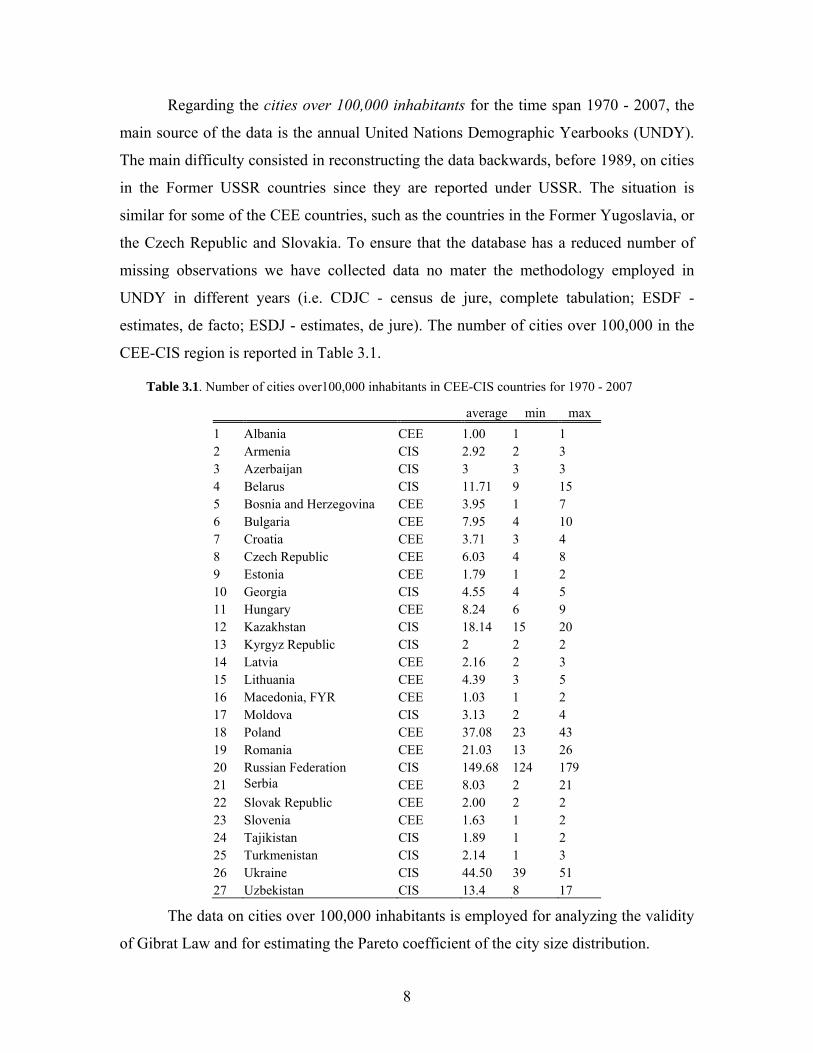
Regarding the cities over 100,000 inhabitants for the time span 1970 - 2007, the

main source of the data is the annual United Nations Demographic Yearbooks (UNDY).

The main difficulty consisted in reconstructing the data backwards, before 1989, on cities

in the Former USSR countries since they are reported under USSR. The situation is

similar for some of the CEE countries, such as the countries in the Former Yugoslavia, or

the Czech Republic and Slovakia. To ensure that the database has a reduced number of

missing observations we have collected data no mater the methodology employed in

UNDY in different years (i.e. CDJC - census de jure, complete tabulation; ESDF -

estimates, de facto; ESDJ - estimates, de jure). The number of cities over 100,000 in the

CEE-CIS region is reported in Table 3.1.

Table 3.1. Number of cities over100,000 inhabitants in CEE-CIS countries for 1970 - 2007

average min max 1 Albania CEE 1.00 1 1 2 Armenia CIS 2.92 2 3 3 Azerbaijan CIS 3 3 3 4 Belarus CIS 11.71 9 15 5 Bosnia and Herzegovina CEE 3.95 1 7 6 Bulgaria CEE 7.95 4 10 7 Croatia CEE 3.71 3 4 8 Czech Republic CEE 6.03 4 8 9 Estonia CEE 1.79 1 2 10 Georgia CIS 4.55 4 5 11 Hungary CEE 8.24 6 9 12 Kazakhstan CIS 18.14 15 20 13 Kyrgyz Republic CIS 2 2 2 14 Latvia CEE 2.16 2 3 15 Lithuania CEE 4.39 3 5 16 Macedonia, FYR CEE 1.03 1 2 17 Moldova CIS 3.13 2 4 18 Poland CEE 37.08 23 43 19 Romania CEE 21.03 13 26 20 Russian Federation CIS 149.68 124 179 21 Serbia CEE 8.03 2 21 22 Slovak Republic CEE 2.00 2 2 23 Slovenia CEE 1.63 1 2 24 Tajikistan CIS 1.89 1 2 25 Turkmenistan CIS 2.14 1 3 26 Ukraine CIS 44.50 39 51 27 Uzbekistan CIS 13.4 8 17

The data on cities over 100,000 inhabitants is employed for analyzing the validity

of Gibrat Law and for estimating the Pareto coefficient of the city size distribution.

9

Regarding the detailed city data, the main source are the national official

statistical information services of CEE and CIS countries. Table 3.2 presents the detailed

data we have acquired so far and that is in various stages of processing.

Table 3.2. Detailed of city data for CEE-CIS countries

Period Level of detail 1 Armenia 1989, 2002, 2008 all cities 2 Azerbaijan 1979, 1989, 2002, 2010 all cities 3 Belarus 1989-2009 all cities 4 Georgia 1989, 2002, 2009 all cities 5 Hungary 1970, 1980, 1990, 2001 all cities and villages

1870, 1880, 1890, 1900, 1910, 1920, 1930, 1940, 1950, 1960, 1970, 1980, 1990, 2000 all cities

6 Kyrgyz Republic 1989, 1999 all cities 7 Latvia 1990 - 2009 all cities 8 Poland 2004 - 2009 all cites 9 Romania 1991, 2002 all cities and villages 10 Russian Federation 1996 - 2004 all cities 11 Serbia 1991, 2002 all cities 12 Slovenia 1981, 1991, 2002 all cities 13 Tajikistan 1989, 1999, 2006 all cities 14 Turkmenistan 1989, 1995, 2006 all cities 15 Ukraine 1989, 2001 2008 all major cities 16 Uzbekistan 1991, 2002, 2006 all cities

The detailed city data is employed for analyzing the validity of Gibrat Law, for

estimating different parametric repartition functions for the city size distribution, and for

analyzing the “within distribution” city dynamics using Markov chains.

Macroeconomic and socio-economic cross-country data is employed in order to

determine the factors that influences of city size distribution. The main sources of data

for this database are World Bank World Development Indicators, Penn World Table, IMF

International Financial Statistics, International Road Federation World Road Statistics,

OECD Telecommunications and Internet Statistics, OECD International Regulation

Database, and national official statistical information services of CEE and CIS countries.

10

4 Methodology

4.1 Testing the validity of Gibrat’s Law

The Gibrat`s law hypothesis is tested by employing both parametric and

nonparametric methods. The simplest parametric test consists in estimating the following

growth equation:

itititit SSS εβα ++=− −− 11 lnlnln (1)

where itS denotes the size of city i at the time t . Gibrat`s law holds if 0=β (i.e.

growth is independent of the initial size). To ensure validity of the statistical results one

must adjust the standard errors of the coefficient estimates for possible dependence in the

residuals. The results of these regressions are usually heteroskedastic (Gonzalez-Val et

al., 2008), so it is suggested in the literature to compute the standard errors using White

Heteroskedasticity-Consistent Covariance Matrix Estimator (White, 1980). However,

another question to be tackled is the presence of cross-sectional dependence in panel data

on city sizes. The cross-sectional dependence is tested using the Pesaran (2004) test,

which does not depend on any particular spatial weight matrix when the cross-sectional

dimension is large. In this paper, to account for the effect of potential cross-correlated

residuals, Driscoll and Kraay (1998) standard errors are employed, Driscoll and Kraay

(1998) modifies the standard Newey and West (1987) covariance matrix estimator such

that it is robust to very general forms of cross-sectional as well as temporal dependences.

Moreover, it is suitable for use with both, balanced and unbalanced panels (Hoechle,

2007).

Clark and Stabler (1991) pointed out that testing for Gibrat’s Law is equivalent to

testing for the presence of a unit root. This idea has also been emphasized by Gabaix and

Ioannides (2004). If the null hypothesis that the city population time series has a unit root

is rejected, the null hypothesis that its size evolves according to Gibrat’s Law is also

rejected. Panel data unit root tests have been proposed as alternative, more powerful tests

than those based on individual time series unit roots tests. The panel unit root approach to

investigate the validity of Gibrat`s Law has been pioneered by Clark and Stabler (1991)

and has already been applied by Davis and Weinstein (2002), Resende (2004), Henderson

and Wang (2007), Soo (2007) and Bosker et al. (2008).

11

Also, when exploring the existence of unit roots in panel data, it is important to

take into account the presence of cross-sectional dependence. Most of these studies

employed conventional (i.e. first generation) unit root tests that assume cross-sectional

independence. The first generation test proposed by Levin, Lin and Chu (2002) is

applicable for homogeneous panels where the coefficients for unit roots are assumed to

be the same across cross-sections. Im, Pesaran and Shin (2003) allows for heterogeneous

panels and proposes panel unit root tests which are based on the average of the individual

ADF unit root tests computed from each time series. The null hypothesis is that each

individual time series contains a unit root, while the alternative allows for some but not

all of the individual series to have unit roots. However, the correct application of these

techniques depends crucially on the assumption that individual time series are cross-

sectional independent. This might be a restrictive assumption when using city size panel

data. Conventional panel unit root tests, such as Levin, Lin and Chu (2002) and Im,

Pesaran and Shin (2003), could lead to significant size distortions in the presence of

neglected cross-section dependence and, generally, to over-rejection of the null

hypothesis.

Much of the recent research on non-stationary panel data has focused on the

problem of cross-sectional dependence. Second generation panel unit root tests that take

into account the potential cross-section dependence in the data have been developed; see

the recent survey by Breitung and Pesaran (2008). A number of panel unit root tests that

allow for cross section dependence have been proposed in the literature that use

orthogonalization type procedures to asymptotically eliminate the cross dependence of

the series before standard panel unit root tests are applied to the transformed series (Bai

and Ng, 2004; Moon and Perron, 2004). On the other hand, Pesaran (2007) suggests a

simple way of accounting for cross-sectional dependence. This method is based on

augmenting the usual ADF regression with the lagged cross-sectional mean and its first

difference to capture the cross-sectional dependence that arises through a single-factor

model. The proposed test has the advantage of being simple and intuitive. It is also valid

for panels where the cross-sample dimension (N) and the time dimension (T) are of the

same orders of magnitudes. The Monte Carlo simulations employed by Pesaran (2007)

12

suggests that the panel unit root tests have satisfactory size and power even for relatively

small values of N and T (i.e. 10<N<200 and 10<T<200).

The present study makes use of a battery of first and second generation panel unit

root tests. More specifically we employ the first generation Levin, Lin and Chu (2002)

and Im, Pesaran and Shin (2003) tests, and the second generation Pesaran (2007) test.

In order to increase the robustness of the results, nonparametric tests are also

implemented. As suggested by Ioannides and Overman (2003) and Eeckhout (2004) for

the non-parametrical analysis of Gibrat’s law it is better to use normalized city growth

rates (i.e. from growth rate of city i in year t the mean is subtracted and the result divided

by the standard deviation of the growth rates). The widely employed Nadaraya-Watson

kernel regression technique (Nadaraya, 1964, 1965; Watson 1964; Hardle, 1992)

establishes a functional form-free relationship between population growth and country

size for the entire distribution. It consists of taking the following specification:

( ) iii smg ε+= (2)

where ig stands for the normalized growth of city i, and is is the logarithm of its

size. Therefore, instead of assuming a linear relationship between these two variables, as

in equation (1), ( )⋅m is estimated as a local average, using a kernel function ( )⋅K :

( )∑

∑

=

=

⎟⎠⎞

⎜⎝⎛ −

⎟⎠⎞

⎜⎝⎛ −

= n

i

i

n

ii

i

NW

hssK

n

gh

ssKnsm

1

1

1

1

(3)

where n is the sample size, and h the kernel bandwidth.

Starting from the estimated mean, ( )⋅NWm , the variance of the growth rate can also

be computed using the corresponding Nadaraya-Watson estimator:

( )( )( )

∑

∑

=

=

⎟⎠⎞

⎜⎝⎛ −

−⎟⎠⎞

⎜⎝⎛ −

= n

i

i

n

iNWi

i

NW

hssK

n

smgh

ssKns

1

1

2

2

1

1

σ (4)

Under the null of urban growth independent of initial size one would expect that

all cities, regardless of their size, have mean normalized growth rate equal to zero and

variance equal to one. These hypotheses are tested by constructing bootstrapped 95-

13

percent confidence bands, calculated from 500 random samples with replacement, as

suggested by González-Val and Sanso-Navarro (2010).

The nonparametric techniques employed in this paper allows computing a variety

of nonparametric and semi-parametric kernel-based estimators appropriate for a mix of

continuous, discrete, and categorical data (Hayfield and Racine, 2008). This kind of non-

parametric technique is convenient because it allows identifying the influence of discrete

variables accounting for possible structural breaks. The basic idea underlying the

treatment of kernel methods in the presence of a mix of categorical and continuous data

lies in the use of generalized product kernels. Li and Racine (2003) proposed the use of

these generalized product kernels for unconditional density estimation and developed the

underlying theory for a data-driven method of bandwidth selection for this class of

estimators. The use of such kernels offers a seamless framework for kernel methods with

mixed data. Further details on a range of kernel methods that employ this approach can

be found in Li and Racine (2007). When all the variables are continuous, these methods

collapse to the familiar Nadaraya-Watson nonparametric regression estimators.

The default Gaussian kernel is employed since the specific form of the local

averaging function does not have a major impact on the results. On the other hand,

bandwidth selection is a key aspect of sound nonparametric kernel regression estimators.

The basic approach in the related urban literature (Eckhout, 2004) is to compute the

bandwidth according to the “rule of thumb” proposed by Silverman (1986) based on

inter-quartile range. In the present study, the bandwidth is selected using a data-driven

method, more specifically, the Kullback - Leibler cross-validated bandwidth selection,

using the method of Hurvich et al. (1998).

4.2 Estimating the Pareto exponent of the city size distribution

The most communally used parametric estimation procedure of the Pareto

exponent is the so called Zipf regression, i.e. regressing the logarithm of the rank of a city

on the logarithm of its size. One potentially serious problem with the Zipf regression is

that it is biased in small samples. Gabaix and Ioannides (2004) show, using Monte Carlo

simulations, that the coefficient of the Zipf regression is biased downward for sample

sizes in the range that is usually considered for city size distributions and that OLS

14

standard errors are grossly underestimated. Therefore, in this paper we employ a

consensus estimate (Graybill and Deal, 1959) of the Pareto exponent using two

alternative econometric methods. The consensus estimate will be weighted with the

inverse of the standard errors of the estimates from the two methods. The first method

(Gabaix and Ibragimov, 2009) consists in a modified Zipf regression:

( ) titit SaR εζ +−=⎟⎠⎞

⎜⎝⎛ − ln

21ln (5)

where iR is the rank of city i in year t. Gabaix and Ibragimov (2009) argue that

the shift of 0.5 is optimal, and reduces the bias to a leading order. They show that the

standard error on the Pareto exponent ζ is not the OLS standard error, but is

asymptotically ( ) ζ21

2n .

The second method, developed in Gabaix and Ioannides (2004) and also

employed by Soo (2005) consists in calculating the value of the Pareto exponent using

the Hill estimator:

( ) ( )( )∑

−

=

−

−= 1

1lnln

1n

ini

H

SS

nζ (6)

Under the null hypothesis of the power law, the Hill estimator is the maximum

likelihood estimator, and it is therefore asymptotically efficient.

4.3 Testing for non-Pareto behavior of the city size distribution

First, as suggested by Rosen and Resnick (1980) we will test for non-Pareto

behavior by include higher order terms of the logarithm of city size in the Zipf

regression:

( ) ( ) ( ) ( ) titititit ScSbSaR εζ +++−= 32 lnlnlnln (7)

and test the statistical significance of their coefficients. However, we must be

cautious of the results, since Gabaix and Ioannides (2004) show that, even if the actual

data exhibit no nonlinear behavior, OLS regression of (7) will yield a statistically

significant coefficient for the quadratic term 78% of the time in a sample of 50

observations.

15

Estimation of parameters in the OLS regression (5) of the logarithm of shifted

rank of the cities on the logarithm of their size will be conducted for 20, 10 and 5

percentage tails of the sample of all cities of the country. This will further allow us to

determine the smallest critical quantity of population for cities in different countries

considered, where Zipf’s Law begins to hold.

We will also consider the non-Pareto behavior of the city size distribution using

alternative parametric models such as the Weber-Fechner Law, whose parameters can be

estimated by using the regression:

( ) titit RS εγβ +−=ln (8)

where the coefficient γ is the so called Weber’s constant, which shows how the

size changes with the change in the rank. In case of the Weber-Fechner law, the rank of

the city changes in arithmetic progression with the change of the size of the city in

geometric progression, while in case of the Zipf’s law both rank and the size of the city

change in arithmetic progression.

In general, Zipf’s law does not hold for small cities (with the size below a cut-

off). Therefore, we expect that the Weber-Fechner law would better describe the whole

sample of all cities and other populated areas in a certain country. It should also be noted

that in terms of statistical characteristics one natural extension of the Weber-Fechner law

is a logarithmic hierarchy model:

iiii NNNNci 4433221 lnlnlnlnln αααα ++++= (9)

where ykln denotes the kth iteration of logarithm (i.e. yyk

k 43421ln...lnlnln = , k≥1).

The authors will further focus on other distributional alternatives, including the

log-normal distribution that was used in several studies to describe the distribution of all

cities in a country (Eeckhout, 2004; Gonzalez-Val et al., 2008). Using several distribution

goodness-of-fit tests (e.g. Kolmogorov-Smirnov, Anderson-Darling) we will determine

the optimal distributional models for the analyzed city size data.

4.4 Studying the “within distribution” city dynamics

Zipf’s and other distribution laws allow the characterization of the evolution of

the global distribution, but they do not provide any information about the movements of

16

the towns within this distribution. A possible way to answer these questions is to track the

evolution of each city’s relative size over time by estimating transition probability

matrices associated with discrete Markov chains. This line of analysis has first been

pursued by Eaton and Eckstein (1997) and then by Black and Henderson (2003).

We assume that the frequency of the distribution follows a first-order stationary

Markov process. In this case, the evolution of the city size distribution is represented by a

transition probability matrix, M, in which each element (i, j) indicates the probability that

a city that was in class i at time t ends up in class j in the following period. The way of

cities’ division on classes will be chosen by considering the performance of the test for

Markovity of order one. Then each element ijp of the transition matrix is estimated as a

conditional probability ( ( 1) | ( ))ij j ip P A t A t= + , where ( )iA t is the event that “city is in a

state i at time t ”. In other words we find shares of cities remained in each size class at the

end of the period and moved up or down by the end of the period. Denoting by

( )1 2( ) ( ) ( )t kF p t p t p t= K the vector of probabilities that a city is in class i at time t

, the dynamics of this vector is given by:

11 0

nn nF F M F M ++ = = (10)

Next, we determine the ergodic distribution that can be interpreted as the long-run

equilibrium city-size distribution. Explicitly, given that the transition matrix M is regular,

then nM tends to a limiting matrix *M when n tends to infinity (Kemeny and Snell,

1960). Therefore, with the passage of time, the distribution of cities will not change any

more and will converge to the ergodic or limit distribution. Concentration of the

frequencies in a certain class would imply convergence (if it is the middle class, it would

be convergence to the mean), while concentration of the frequencies in some of the

classes, that is, a multimodal limit distribution, may be interpreted as a tendency towards

stratification into different convergence clubs. Finally, a dispersion of this distribution

amongst all classes is interpreted as divergence.

We also determine the speed of the movement of a city within the distribution,

using the mean first passage time matrix PM , that can be easily constructed for the

transition matrix M (Kemeny and Snell, 1976). The (i,j) element of the matrix PM

indicates the expected time for a city to move from class i to class j for the first time.

17

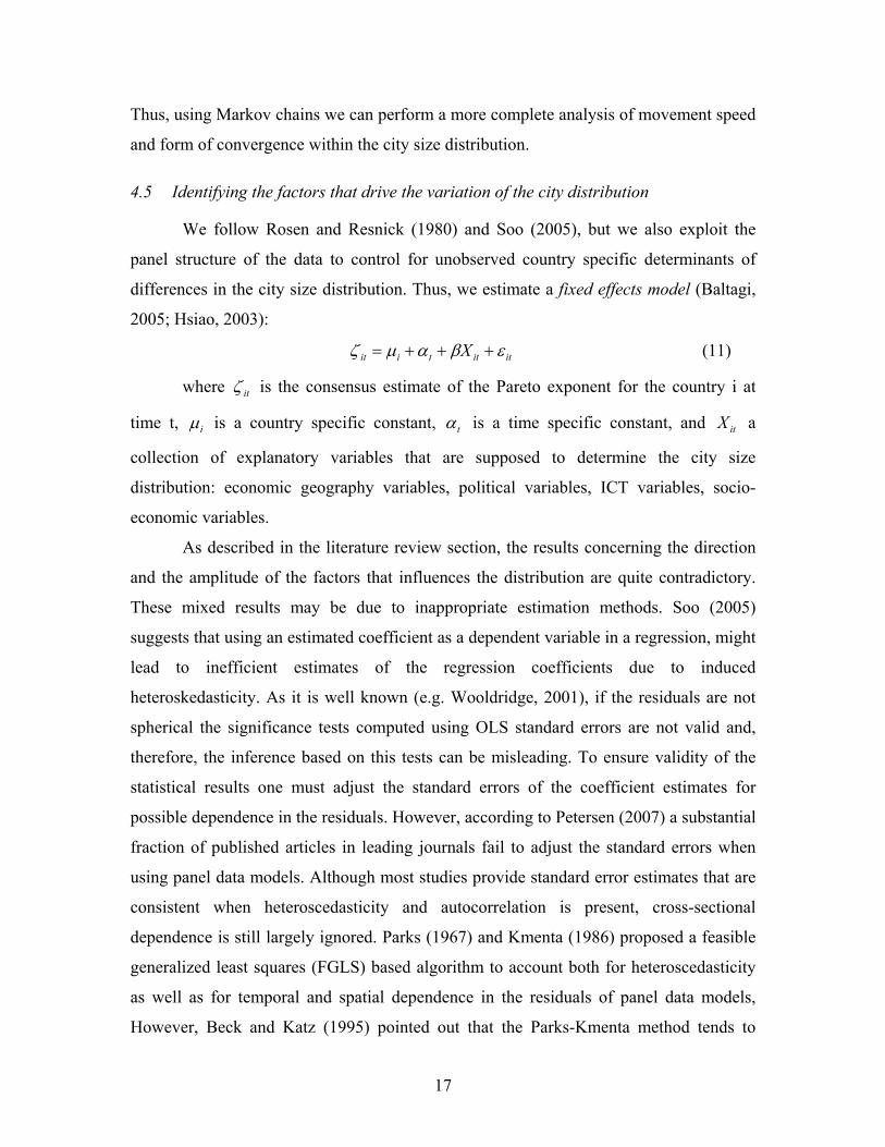
Thus, using Markov chains we can perform a more complete analysis of movement speed

and form of convergence within the city size distribution.

4.5 Identifying the factors that drive the variation of the city distribution

We follow Rosen and Resnick (1980) and Soo (2005), but we also exploit the

panel structure of the data to control for unobserved country specific determinants of

differences in the city size distribution. Thus, we estimate a fixed effects model (Baltagi,

2005; Hsiao, 2003):

itittiit X εβαμζ +++= (11)

where itζ is the consensus estimate of the Pareto exponent for the country i at

time t, iμ is a country specific constant, tα is a time specific constant, and itX a

collection of explanatory variables that are supposed to determine the city size

distribution: economic geography variables, political variables, ICT variables, socio-

economic variables.

As described in the literature review section, the results concerning the direction

and the amplitude of the factors that influences the distribution are quite contradictory.

These mixed results may be due to inappropriate estimation methods. Soo (2005)

suggests that using an estimated coefficient as a dependent variable in a regression, might

lead to inefficient estimates of the regression coefficients due to induced

heteroskedasticity. As it is well known (e.g. Wooldridge, 2001), if the residuals are not

spherical the significance tests computed using OLS standard errors are not valid and,

therefore, the inference based on this tests can be misleading. To ensure validity of the

statistical results one must adjust the standard errors of the coefficient estimates for

possible dependence in the residuals. However, according to Petersen (2007) a substantial

fraction of published articles in leading journals fail to adjust the standard errors when

using panel data models. Although most studies provide standard error estimates that are

consistent when heteroscedasticity and autocorrelation is present, cross-sectional

dependence is still largely ignored. Parks (1967) and Kmenta (1986) proposed a feasible

generalized least squares (FGLS) based algorithm to account both for heteroscedasticity

as well as for temporal and spatial dependence in the residuals of panel data models,

However, Beck and Katz (1995) pointed out that the Parks-Kmenta method tends to

18

produce unacceptably small standard error estimates, and they introduced the method of

panel corrected standard errors (PCSE). Soo (2005) in his cross-country study on city size

distributions advocates the use OLS coefficient estimates with panel corrected standard

errors. Nevertheless, Driscoll and Kraay (1998) and Hoechle (2007) points out that the

finite sample properties of the PCSE estimator are rather poor when the panel’s cross-

sectional dimension N is large compared to the time dimension T. Driscoll and Kraay

(1998) demonstrate that this problem can be solved by modifying the standard Newey

and West (1987) covariance matrix estimator such that it is robust to very general forms

of cross-sectional as well as temporal dependences. Moreover, it is suitable for use with

both, balanced and unbalanced panels. In this paper we employ Driscoll-Kraay standard

errors in order to ensure valid statistical inference

Following Ioannides et al. (2008), in order to ensure the robustness of the results,

we intent to employ other measures of urban concentration as dependent variable in

equation (11): the coefficient of variation, the Gini index, and the normalized Herfindahl

concentration index. These measures, that are computed using the consensus estimate of

the Pareto exponent, reflect different aspects of dispersion.

5 Results

5.1 Results concerning Gibrat Law

In this section Gibrat`s law is investigated using two datasets of cites from

transition economies. The first dataset consists in detailed city size data from Poland,

Belarus and Latvia for the period 2000-2009. More specifically, in the case of Poland the

largest 200 cities are considered, in Belarus the largest 50 cities, and in Latvia the largest

30 cities. The main source of the detailed data is the national official statistical

information services of the respective countries. The second dataset is focused on data for

the period 1970 – 2007 on cities over 100,000 inhabitants from twelve transition

economies, namely Russia, Ukraine, Poland, Romania, Belarus, Bulgaria, Hungary,

Czech Republic, Slovak Republic, Estonia, Latvia and Lithuania.

19

Five of the countries are pooled into two groups, since there is a relatively low cross-

section dimension when analyzed separately. The first group consists of the Baltic States

(Estonia, Latvia, Lithuania), the second one of the countries from the Former

Czechoslovakia (Czech Republic, Slovak Republic). The average number of cities over

100,000 inhabitants for the remaining units is as follows: Russian Federation 152,

Ukraine 45, Poland 37, Romania 21, Belarus 12, Bulgaria 8, Hungary 8, Former

Czechoslovakia 8, and Baltic States 8.

Table A.5.1.1 in the Appendix describes the dataset, presenting the number of

observations, the time and cross-section dimensions of the panel, the average, standard

deviation, minimum and maximum city size.

5.1.1 Gibrat`s law for detailed city data In this subsection the analysis is conducted on the dataset containing detailed city

size data in Poland, Belarus and Latvia for the period 2000 – 2009. Pooling observations

and using panel data methods is a necessary strategy to increase the reliability of the

estimates when the observed period is relatively short (Banerjee, 1999). First, the growth

equation (1) was estimated using both pooled data and a fixed effects panel model. The

results of these estimations are presented in the first two lines of Table 5.1.1. In the urban

literature, to test the significance of the parameters, White (1982) standard errors are

generally employed since they are robust to heteroskedastic innovations. However, in this

case, the estimated regression residuals of the fixed effects model are cross-sectionally

dependent, as is clearly noticeable in the third line from Table 5.1.1. The pair-wise cross-

section correlations coefficients of the residuals are not zero, since the average absolute

correlation between the residuals of two cities is 0.318 in Poland, 0.39 in Belarus, and

0.341 in Latvia. Also, Pesaran (2004) cross-sectional dependence test rejects the null

hypothesis of spatial independence on any standard level of significance. Therefore, this

finding indicates that it is advisable to test for significance using Driscoll and Kraay

(1998) standard errors, since they are robust to very general forms of cross sectional and

temporal dependence.

20

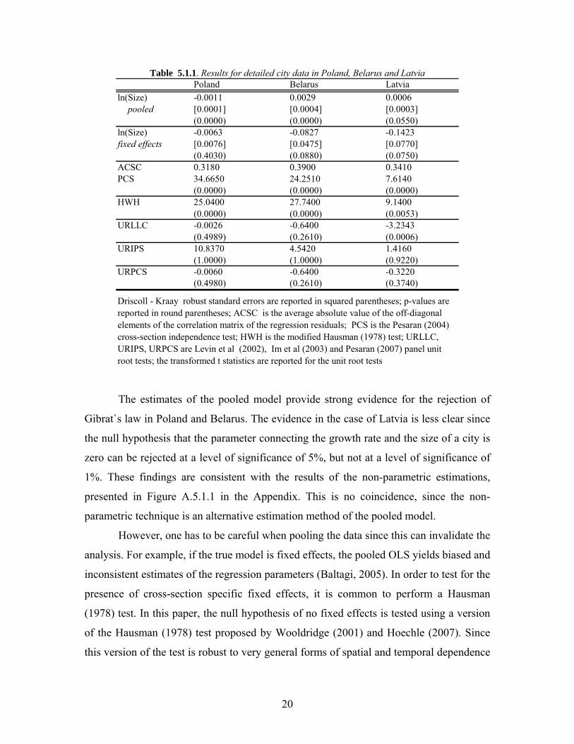
Table 5.1.1. Results for detailed city data in Poland, Belarus and Latvia Poland Belarus Latvia

ln(Size) -0.0011 0.0029 0.0006pooled [0.0001] [0.0004] [0.0003]

(0.0000) (0.0000) (0.0550)ln(Size) -0.0063 -0.0827 -0.1423fixed effects [0.0076] [0.0475] [0.0770]

(0.4030) (0.0880) (0.0750)ACSC 0.3180 0.3900 0.3410PCS 34.6650 24.2510 7.6140

(0.0000) (0.0000) (0.0000)HWH 25.0400 27.7400 9.1400

(0.0000) (0.0000) (0.0053)URLLC -0.0026 -0.6400 -3.2343

(0.4989) (0.2610) (0.0006)URIPS 10.8370 4.5420 1.4160

(1.0000) (1.0000) (0.9220)URPCS -0.0060 -0.6400 -0.3220

(0.4980) (0.2610) (0.3740)

Driscoll - Kraay robust standard errors are reported in squared parentheses; p-values are reported in round parentheses; ACSC is the average absolute value of the off-diagonal elements of the correlation matrix of the regression residuals; PCS is the Pesaran (2004) cross-section independence test; HWH is the modified Hausman (1978) test; URLLC, URIPS, URPCS are Levin et al (2002), Im et al (2003) and Pesaran (2007) panel unit root tests; the transformed t statistics are reported for the unit root tests

The estimates of the pooled model provide strong evidence for the rejection of

Gibrat`s law in Poland and Belarus. The evidence in the case of Latvia is less clear since

the null hypothesis that the parameter connecting the growth rate and the size of a city is

zero can be rejected at a level of significance of 5%, but not at a level of significance of

1%. These findings are consistent with the results of the non-parametric estimations,

presented in Figure A.5.1.1 in the Appendix. This is no coincidence, since the non-

parametric technique is an alternative estimation method of the pooled model.

However, one has to be careful when pooling the data since this can invalidate the

analysis. For example, if the true model is fixed effects, the pooled OLS yields biased and

inconsistent estimates of the regression parameters (Baltagi, 2005). In order to test for the

presence of cross-section specific fixed effects, it is common to perform a Hausman

(1978) test. In this paper, the null hypothesis of no fixed effects is tested using a version

of the Hausman (1978) test proposed by Wooldridge (2001) and Hoechle (2007). Since

this version of the test is robust to very general forms of spatial and temporal dependence

21

it should be suitable for the case of city size panel data. The results of the tests are

presented in the fourth line of Table 5.1.1. They provide strong evidence in the favor of

the fixed effects model because the null of no fixed effects is rejected at any usual level

of significance. The estimates from the fixed effects model provide contrary evidence to

that indicated by the pooled data model. As it turns out, when accounting for city specific

effects, the null hypothesis of cities growing independent of their size can not be rejected

at the level of 5% for any of the three countries.

Next, the panel structure of the city population data is further exploited in order to

test for a unit root. Although only 10 observations over time are available, the use of a

panel unit root test with a relatively large cross-section dimension is likely to alleviate the

small-sample bias of a usual ADF unit root test. Black and Henderson (2003) also

employs 10 time observation (decade by decade) in their study on urban evolution in the

USA. Following Clark and Stabler (1991) only a constant has been included as the

deterministic term. The results for the first generation Levin, Lin and Chu (2002) and Im,

Pesaran and Shin (2003) tests, and the second generation Pesaran (2007) test are reported

in the last three lines of Table 5.1.1.

Although, the first generation tests are used for completeness, more weight is

given to the test of Pesaran (2007) since it allows investigating the presence of a unit root

taking into account cross-sectional dependence, which is the case of the analyzed sample.

Moreover, the test is robust to size distortions caused by the potential presence of serially

correlated errors. As one can easily notice, the test can not reject the null of a unit root at

any usual level of significance, therefore, providing support for the acceptance of

Gibrat`s law in all the three countries.

However, it has to be stressed that, since specific city effects are taken into

account, the deterministic component (the expected growth rate) is different across cities.

Therefore, although the coefficient that quantifies the influence of the size on growth is

zero, a consistent difference in the expected growth rate between “small” cities and

“large” cities might indicate that Gibrat`s law does not hold. This could be the case of

Belarus, because the non-parametric analysis indicates that there are differences between

the behavior of small cities, medium cities and large cities.

22

To investigate further, the cities in Belarus are grouped in three categories,

respectively the “large” cities group consisting of the largest 8 cities, the “medium” group

comprising the next largest 27 cities, and the “small” group with the last 15 cities. The

grouping was done such that the modified Hausman (1978) test indicates that for each of

the group a pooled model is adequate. There is a significant difference between the

average growth rates of the cities in these groups, with an average annual growth of

0.49% for the first group, -0.15% for the second group, and -0.46% for the small cities

group. Therefore, a growth regression was estimated for each of the group, and another

one for the entire sample but controlling for group specific characteristics. The results are

reported in Table A.5.1.2 in the Appendix. It seems that for the large cities group there is

a significant dependence of growth on size. Moreover, after the dummy variables

controlling for different groups are accounted for, the coefficient quantifying the

dependence of the size of the city on its growth rate is statistically significant at 5%. This

finding proves the validity of intuitive doubts as to proportionality of growth in Belarus

where the intentionally designed redistribution measures are evident.

Overall, in the period 2000-2009 there is very strong evidence that Gibrat`s law

holds for Latvia and strong evidence that in is valid in Poland. However, it seems that, at

least in the short run, there is a divergence pattern in the case of Belarus. A longer time

span is necessity for a deeper investigation of the long run dynamics of city growth.

5.1.2 Gibrat`s law for cities over 100,000 inhabitants

In this subsection the analysis turns to cities over 100,000 inhabitants in the

period 1970 – 2007. There are twelve countries in the sample, but, after pooling some of

them as described above, nine units remain, respectively Russia, Ukraine, Poland,

Romania, Belarus, Bulgaria, Hungary, Former Czechoslovakia, and Baltic States.

A major problem with this dataset is the existence of missing observations.

Although, data were collected irrespective of the methodology employed in the UNDY in

different years, Hungary is the only country in the sample that has all the 38 observations

over time. In the Baltic States there are 32 time observations, in Bulgaria 28, in Belarus

23

and Poland 27, in Romania 26, in Former Czechoslovakia 25, in Russia 24, and in

Ukraine only 17. Moreover, since growth rates are needed in our analysis, the problem of

missing data is further amplified since the growth rate can not be computed if consecutive

year data is not available. When estimating the growth regression using pooled data or

the fixed effects model, an assumption had to be made in order to alleviate this problem

of missing growth rates. More specifically, if city sizes data is missing in year t, but not

in year t-1, the growth rate of a city for the period t/t-1 is, however, computed by

assuming to be equal to the annual average growth rate between year t and the year with

the next available city sizes data. This is a reasonable assumption since it does not

introduce new city data by interpolation. It uses only the original city size data, but it

computes the growth rates with different formulas depending on the situation.

First, the growth equation (1) was estimated using both pooled data and a fixed

effects panel model. To capture the influence of the breakdown of the communist regime

the sample is also divided in two subsamples, respectively 1970-1989 and 1990-2007.

The results are reported in Table 5.1.2. The null of no fixed effects can not be rejected at

the level of significance of 1% for any of the countries. Although, the results of the fixed

effects model are reported for completeness, more weight should be, therefore, given to

the pooled model in this case. To ensure that the panels are balanced some of the cities

with sparse observations were drooped. Therefore, the number of analyzed cities is 108

for Russia, 31 for Ukraine, 23 for Poland, 13 for Romania, 9 for Belarus, and 6 for

Bulgaria, Hungary, Former Czechoslovakia and the Baltic States. The average absolute

value of the off-diagonal elements of the correlation matrix of the regression residuals

varies from 31.7% for Poland to 72.6% for Romania. Also, the null hypothesis of cross-

sectional independence is rejected for all the countries, implying the necessity of using

Driscoll and Kraay (1998) standard errors to correct for cross sectional dependence.

The results of the pooled regression indicates that, in the post-communist period,

Gibrat`s law is valid in all of the countries, with some doubts in the case of Hungary.

When all the sample is considered the evidence for accepting Gibrat`s law is less clear in

Russia, Ukraine, Poland, and Romania. These findings are largely confirmed by the

results of the non-parametrical regressions that are provided in Table A.5.1.2 in the

Appendix. However, these results indicate that there is strong support for the law of

24

proportional effect in the case of Russia and Ukraine, when the entire sample is

considered.

Table 5.1.2.. Growth regressions results for cities over 100,000 inhabitants for the period 1970-2007 Pooled regression HWH Fixed effects regression ACSC PCS

estim. std. err. p-value estim. std. err. p-value statistic p-valueRussia all sample -0.0060 0.0027 0.0265 5.7100 -0.2052 0.0655 0.0022 0.3800 100.58 0.0000

before 1989 -0.0036 0.0010 0.0003 (0.0186) -0.1499 0.0633 0.0196 0.6350 135.03 0.0000after 1989 -0.0065 0.0044 0.1418 -0.4061 0.0591 0.0000 0.4910 38.66 0.0000

Ukraine all sample -0.0094 0.0039 0.0231 6.3300 -0.1645 0.0563 0.0065 0.5050 41.63 0.0000before 1989 -0.0046 0.0020 0.0269 (0.0175) -0.0715 0.0080 0.0000 0.3680 9.91 0.0000after 1989 -0.0114 0.0078 0.1560 -0.3873 0.0524 0.0000 0.6920 41.56 0.0000

Poland all sample -0.0031 0.0015 0.0443 4.4200 -0.0859 0.0239 0.0016 0.3170 23.14 0.0000before 1989 -0.0042 0.0014 0.0085 (0.0472) -0.0676 0.0288 0.0282 0.2620 11.35 0.0000after 1989 0.0008 0.0019 0.6617 -0.1881 0.1236 0.1423 0.5280 15.65 0.0000

Romania all sample -0.0065 0.0023 0.0146 8.0600 -0.0741 0.0249 0.0117 0.7260 21.27 0.0000before 1989 -0.0048 0.0017 0.0176 (0.0149) -0.0241 0.0234 0.3242 0.7990 26.39 0.0000after 1989 0.0013 0.0008 0.1614 -0.0924 0.0426 0.0510 0.7490 33.06 0.0000

Belarus all sample -0.0053 0.0034 0.1524 2.8500 -0.1516 0.0867 0.1186 0.5500 16.42 0.0000before 1989 -0.0101 0.0067 0.1695 (0.1299) -0.2295 0.1360 0.1300 0.7660 12.84 0.0000after 1989 -0.0001 0.0018 0.9644 -0.4539 0.1107 0.0034 0.4370 8.55 0.0000

Bulgaria all sample -0.0016 0.0026 0.5666 0.6500 -0.0635 0.0174 0.0148 0.3450 5.77 0.0000before 1989 -0.0015 0.0032 0.6482 (0.4576) -0.0470 0.0099 0.0051 0.3830 4.59 0.0000after 1989 0.0013 0.0037 0.7402 -0.2676 0.0599 0.0066 0.4050 2.04 0.0416

Hungary all sample -0.0046 0.0018 0.0515 5.7800 -0.1440 0.0433 0.0209 0.5300 12.10 0.0000before 1989 -0.0052 0.0029 0.1403 (0.0613) -0.1994 0.0339 0.0020 0.2730 3.23 0.0012after 1989 -0.0040 0.0014 0.0353 -0.0859 0.0764 0.3121 0.7070 11.62 0.0000

Fr. Czechosl. all sample -0.0040 0.0021 0.1214 3.0200 -0.0874 0.0289 0.0293 0.6580 12.49 0.0000before 1989 -0.0068 0.0021 0.0234 (0.1430) -0.0540 0.0347 0.1803 0.6430 8.63 0.0000after 1989 0.0010 0.0009 0.3523 -0.0909 0.0537 0.1514 0.5350 7.18 0.0000

Baltic States all sample -0.0030 0.0014 0.0888 5.2600 -0.0953 0.0188 0.0039 0.6240 13.46 0.0000before 1989 -0.0014 0.0011 0.2796 (0.0703) -0.0508 0.0047 0.0001 0.2050 2.51 0.0122after 1989 -0.0021 0.0016 0.2510 -0.0359 0.0253 0.2162 0.3500 4.41 0.0000

std. err. are Driscoll - Kraay robust standard errors; ACSC is the average absolute value of the off-diagonal elements of the correlation matrix of the regression residuals of the fixed effects model; PCS is the Pesaran (2004) cross-section independence test; HWH is the modified Hausman (1978) test for the case when all the sample is considered; p-values are reported in round parentheses.

Next, the analysis turns to investigating the presence of a unit root taking into

consideration the panel structure of the data. When using classical panel data techniques,

the growth rates and the city sizes can be looked at as two different inputs and the

procedure for filling some of the missing growth rates described above is employed.

However, an even major problem arises when the unit root tests are considered. In this

case, the input consists only in the city size data. Testing for a unit root in a time series

with missing observations has received little attention in the econometric literature. Shin

and Sarkar (1996) tested for a unit root in a AR(1) time-series using irregularly observed

data and obtain the limiting distributions associated with the case where the gaps are

25

ignored (i.e. the series are closed), and with the case where the gaps are replaced with the

last available observation. They show that replacing the gaps with the last observation, or

simply ignoring the gaps, does not alter the usual asymptotic results associated with DF

statistics. Shin and Sarkar (1996) also investigated the finite sample properties of the two

alternatives of dealing with missing observations in the case of an “A-B sampling

scheme”, where A is the number of available observations and B is the number of

missing observations. Their simulation results show that the unit root test performs

relatively well in small samples. Shin and Sarkar (1994) investigated a unit root test for

an ARIMA(0,1,q) model with irregularly observed sample and prove to have the same

asymptotic distribution as the DF statistics for the complete data situation. Some

simulation results for the ARIMA(0,1,1) model show that the sizes of the tests for A-B =

6-1, 5-2 and 4-3 were similar to those for the case where there are no missing

observations (i.e. A-B=7-0).

When dealing with time series data with missing observations, the other most

common technique besides ignoring the gaps, and replacing the gaps with the last

available observation, consists in filling the gaps with a linear interpolation method. It

could be argued that instead of using the last available observation to fill these gaps, a

linear interpolation between the known observations could provide a “smoother”

alternative of dealing with gaps. However, the distributional implications of such a

procedure require careful consideration, even in large samples. Giles (1999) extended the

results of Shin and Sarkar (1996) and investigated the behavior of unit root tests when a

linear interpolation method for dealing with the gaps in the data is employed. They prove

that the limiting distribution includes an adjustment factor which results in critical values

that are less negative than for the usual DF statistic. Giles (1999) also investigated the

finite sample properties of the three alternatives for dealing with missing data. The

findings obtained by Giles (1999) within a simulation experiment framework indicate

that the unit root tests are more powerful when gaps are ignored, as compared with the

other two alternatives of filling missing data. Following Giles (1999), when testing for a

unit root in the case of cities over 100,000 inhabitants, the gaps are ignored. The results

are reported in Table 5.1.3.

26

Table 5.1.3. Unit root tests results for cities over 100,000 inhabitants for the period 1970-2007 URLLC URIPS URPCS

statistic pvalue statistic pvalue statistic p-value statistic bkp.Russia all sample -10.5586 0.0000 -6.5340 0.0000 2.3070 0.9890 Russia

before 1989 -27.8783 0.0000 -10.7660 0.0000 -0.9860 0.1620 average -3.8670 1999after 1989 -12.1703 0.0000 -4.9730 0.0000 -6.6840 0.0000 max -4.5920 2002

Ukraine all sample -2.5530 0.0053 0.9990 0.8410 1.0150 0.8450 Ukraine before 1989 - - - - - - average -4.1640 1993after 1989 - - - - - - max -6.0970*** 1985

Poland all sample -4.0467 0.0000 -1.6410 0.0500 -1.3670 0.0860 Poland before 1989 -4.6524 0.0000 -0.6220 0.2670 -0.7110 0.2390 average -4.2310 1987after 1989 -5.9089 0.0000 0.1470 0.5580 0.0350 0.5140 max -3.5700 1990

Romania all sample -3.9243 0.0000 -2.2200 0.0130 -2.7190 0.0030 Romania before 1989 -1.1504 0.1250 1.5330 0.9370 -2.0380 0.0210 average -3.2650 1981after 1989 0.1505 0.5598 -0.8680 0.1930 1.3510 0.9120 max -1.9660 1995

Belarus all sample -4.5845 0.0000 -3.5480 0.0000 -0.8670 0.1930 Belarus before 1989 -4.0950 0.0000 -0.3580 0.3600 -2.0620 0.0200 average -5.5840*** 1989after 1989 -2.2261 0.0130 -0.0920 0.4630 1.0640 0.8560 max -34.1120*** 1999

Bulgaria all sample -0.8885 0.1871 -0.4400 0.3300 -1.0940 0.1370 Bulgaria before 1989 -0.6097 0.2710 0.5820 0.7200 -1.0400 0.1490 average -3.8340 1984after 1989 2.8549 0.9978 3.1260 0.9990 -0.6410 0.2610 max -4.5170 1978

Hungary all sample -2.6283 0.0043 -5.2390 0.0000 -2.9440 0.0020 Hungary before 1989 -6.7794 0.0000 -6.0500 0.0000 -3.5510 0.0000 average -4.7470 1978after 1989 -2.2863 0.0111 -1.4060 0.0800 -0.7280 0.2330 max -4.2150 1994

Fr. Czechosl. all sample -6.1552 0.0000 -4.6060 0.0000 -0.9050 0.1830 Fr. Czechoslbefore 1989 -1.7602 0.0392 0.8580 0.8040 -0.2510 0.4010 average -3.1240 1985after 1989 -2.8482 0.0022 -0.4750 0.3180 -1.0010 0.1580 max -2.0380 1997

Baltic States all sample -1.2091 0.1133 1.0560 0.8540 1.1210 0.8690 Baltic Statesbefore 1989 -0.4943 0.3105 0.9690 0.8340 -1.2810 0.1000 average -4.2770 1982after 1989 -4.5589 0.0000 -2.0140 0.0220 0.6400 0.7390 max -2.8640 1993

ZA

URLLC is the Levin et al (2002) panel unit root test; URIPS is the Im et al (2003) panel unit root test; URPCS is the Pesaran (2007) panel unit root test; the transformed t statistics are reported for the panel unit root tests; ZA is the Zivot and Andrews (1992) unit toot test wit structural breaks, bkp. indicates the year a breakpoint was detected ; *,** and *** denotes statistical significance at 10%, 5% and 1% level .

Again, in order to ensure a balanced panel, the analysis focuses on 108 cities in

Russia, 31 in Ukraine, 23 in Poland, 13 in Romania, 9 in Belarus, and 6 for Bulgaria,

Hungary, Former Czechoslovakia and the Baltic States. The unit root tests are not

conducted unless at least 10 time observations are available, which is the case of Ukraine

when the sample is split in the two sub-periods. When the tests indicate contradictory

results, the priority is given to Pesaran (2007) test since it is robust to cross-sectional

dependence. The results confirm, in general, the findings of the growth regressions. More

specifically, the unit root tests indicate that, after 1989, the Gibrat`s law is valid in all the

countries except Russia.

There is one major caveat of the regressions and of the unit root tests analyzed so

far. That is the existence, after 1989, of a potential change in the deterministic component

27

of the growth rates of the cities in the former communist block, at which the analysis is

focused on in the next subsection.

5.1.3 Accounting for a potential structural break in 1989

First, the effect of a potential break on the previous results on the unit roots test is

investigated. Regarding unit root tests, Perron (1989) pointed out that failure to account

for an existing break leads to a bias resulting in an under-rejection of the unit root null

hypothesis. To overcome this problem, Perron (1989) proposed allowing for an

exogenous structural break in the standard ADF tests. Following this breakthrough,

several authors including, Zivot and Andrews (1992) and Perron (1997) proposed

determining the break point endogenously from the data. To account for a possible break

in the series, a Zivot and Andrews (1992) unit root test was conducted. For each country,

the largest city and a hypothetical city with the size equal to the average city size in the

respective country were investigated. The last column in Table 5.1.3 reports the results.

Zivot and Andrews (1992) structural break test is a sequential test which employs the full

sample and a different dummy variable for each possible break date. The break date is

selected at the time where the t-statistic of the ADF test is at a minimum, therefore, where

the evidence is least favorable for the unit root hypothesis. Even accounting for a

potential break, the hypothesis of a unit root, in the case of the “average” city, could not

be rejected for any of the countries, except Belarus. This finding provides strong

evidence in favor of Gibrat`s law.

When estimating the growth regressions in the previous subsection, the sample

was split in two sub-periods to account for a possible change in the fulfillment of Gibrat`s

law. However, it could be argued that splitting the data into subsets may lead to a loss in

efficiency due to the reduction in the sample size. Therefore, another alternative to

control for a potential change in the deterministic component of the growth rates of the

cities is also employed. More specifically, a dummy variable, taking the value zero before

1989 and the value one afterwards, is introduced in the growth regressions. The results

are reported in Table 5.1.4.

28

Table 5.1.4. Structural breaks in the growth regressions for cities over 100,000 inhabitants for the period 1970-

2007

Russia Ukraine Poland Romania Belarus Bulgaria Hungary Fr. Czechosl. Baltic Statesln(Size) -0.0054 -0.0078 -0.0023 -0.0016 -0.0034 0.0002 -0.0045 -0.0031 -0.0017

[0.0027] [0.0038] [0.0014] [0.0012] [0.0029] [0.0023] [0.0018] [0.0018] [0.0009](0.0491) (0.0473) (0.1109) (0.2316) (0.2764) (0.9261) (0.0548) (0.1460) (0.1294)

postcom -0.0156 -0.0256 -0.0156 -0.0302 -0.0167 -0.0210 -0.0218 -0.0152 -0.0269[0.0035] [0.0084] [0.0030] [0.0078] [0.0096] [0.0042] [0.0051] [0.0037] [0.0028](0.0000) (0.0047) (0.0000) (0.0022) (0.1190) (0.0040) (0.0079) (0.0096) (0.0002)

Russia Ukraine Poland Romania Belarus Bulgaria Hungary Fr. Czechosl. Baltic Statesln(Size) -0.2144 -0.1549 -0.0683 -0.0296 -0.2122 -0.0332 -0.1378 -0.0631 -0.0424

[0.0708] [0.0605] [0.0236] [0.0206] [0.1217] [0.0199] [0.0336] [0.0276] [0.0074](0.0031) (0.0157) (0.0084) (0.1760) (0.1193) (0.1552) (0.0093) (0.0707) (0.0023)

postcom 0.0063 -0.0057 -0.0100 -0.0232 0.0347 -0.0152 -0.0206 -0.0096 -0.0234[0.0092] [0.0090] [0.0018] [0.0072] [0.0235] [0.0051] [0.0037] [0.0024] [0.0021](0.4962) (0.5324) (0.0000) (0.0073) (0.1785) (0.0307) (0.0024) (0.0097) (0.0001)

ACSC 0.3850 0.5010 0.2230 0.7930 0.5470 0.3280 0.3590 0.6080 0.3240PCS 102.1650 40.8250 13.1820 34.9980 15.8190 5.2890 8.1830 11.5450 6.1380

(0.0000) (0.0000) (0.0000) (0.0000) (0.0000) (0.0000) (0.0000) (0.0000) (0.0000)

Pooled regression

Fixed effects regression

postcom is a dummy variable taking the value zero before 1989 and the value one aftewards; Driscoll - Kraay robust standard errors are reported in squared parentheses; p-values are reported in round parentheses; ACSC is the average absolute value of the off-diagonal elements of the correlation matrix of the regression residuals of the fixed effects model; PCS is the Pesaran (2004) cross-section independence test

The estimates of the pooled data model, which, as argued in the previous

subsection, is given priority over the fixed effects model, indicate that the coefficients of

the variable accounting for a change in the deterministic component are significantly

different from zero in all the countries, except Belarus. As already mentioned, the non-

parametric techniques employed in this paper (Li and Racine 2003; Hayfield and Racine,

2008) are appropriate for a mix of continuous and discrete data. This is convenient

because it allows investigating, by means of non-parametric regression, whether the

influence of discrete variables accounting for potential structural breaks is significant.

The graphs in Figure 5.1.1 depict the impact on city growth rates of the dummy

variable accounting for a structural break in 1989. As it is standard in non-parametric

analysis, to capture the sole influence of one variable (in this case the dummy), the other

variable (in this case the relative city size) is held at the median value. The 95%

distribution free (bootstrapped) error bounds, computed using 500 random samples with

replacement, are also depicted. The results confirm the findings of the parametric analysis

with a shift in the deterministic component detected in all the countries except Belarus.

29

Figure 5.1.1. The non-parametrical estimates of the potential shift in the deterministic component of

growth rates

before after

0

before after

0

before after

0

a. Russia b. Ukraine c. Poland

before after

0

before after

0

before after

0

d. Romania e. Belarus f. Bulgaria

before after

0

before after

0

before after

0

g. Hungary h. Former Czechoslovakia i. Baltic States

After the influence of the change in the deterministic component is accounted for,

the null hypothesis of the validity of Gibrat`s law can not be rejected at any standard level

of significance for six of the analyzed countries or groups of countries, respectively

Poland, Romania, Belarus, Bulgaria, Former Czechoslovakia, and the Baltic States. For

Hungary can not be rejected at 5%, and for Russia and Ukraine cannot be rejected at 1%.

5.1.4 Gibrat`s law using five years averages

Another caveat of the analysis using yearly data on cities over 100,000 inhabitants

is given by the existence of missing data in some of the years in the time span. As argued

in the previous subsections, the treatment of missing data in this study is reasonable and

the consistency of econometric methods assured. However, in order to check the

robustness of the results, in this subsection the analysis is also conducted using five years

30

averages. For the last period, 2005-2007, only three years are available and, therefore,

three years averages are employed.

Table 5.1.5. Growth regressions results for cities over 100,000 inhabitants using five years averages for the period 1970-2007

Pooled regression Pooled regression with dummyall sample before 1989 after 1989 all sample

Russia ln(Size) -0.0023 -0.0020 -0.0006 ln(Size) -0.0012 postcom -0.0175[0.0008] [0.0003] [0.0004] [0.0005] [0.0034](0.0034) (0.0000) (0.1618) (0.0097) (0.0000)

Ukraine ln(Size) -0.0072 -0.0057 -0.0050 ln(Size) -0.0053 postcom -0.0212[0.0019] [0.0010] [0.0023] [0.0013] [0.0047](0.0004) (0.0000) (0.0387) (0.0002) (0.0001)

Poland ln(Size) -0.0032 -0.0058 0.0013 ln(Size) -0.0019 postcom -0.0166[0.0025] [0.0011] [0.0013] [0.0022] [0.0041](0.2127) (0.0000) (0.3107) (0.3946) (0.0005)

Romania ln(Size) -0.0087 -0.0090 0.0010 ln(Size) -0.0036 postcom -0.0314[0.0041] [0.0008] [0.0008] [0.0026] [0.0087](0.0536) (0.0000) (0.2599) (0.1817) (0.0029)

Belarus ln(Size) -0.0032 0.0000 0.0026 ln(Size) 0.0015 postcom -0.0287[0.0018] [0.0031] [0.0015] [0.0010] [0.0031](0.1159) (0.9969) (0.1282) (0.1467) (0.0000)

Bulgaria ln(Size) -0.0001 0.0001 0.0019 ln(Size) 0.0021 postcom -0.0159[0.0013] [0.0011] [0.0034] [0.0018] [0.0037](0.9265) (0.9256) (0.5956) (0.2939) (0.0049)

Hungary ln(Size) -0.0002 -0.0035 0.0006 ln(Size) -0.0008 postcom -0.0133[0.0008] [0.0008] [0.0002] [0.0010] [0.0036](0.8148) (0.0088) (0.0242) (0.4320) (0.0099)

Fr. Czechosl. ln(Size) -0.0039 -0.0068 0.0005 ln(Size) -0.0028 postcom -0.0148[0.0023] [0.0011] [0.0005] [0.0020] [0.0039](0.1525) (0.0017) (0.3546) (0.2157) (0.0125)

Baltic States ln(Size) -0.0028 -0.0011 -0.0014 ln(Size) -0.0013 postcom -0.0218[0.0008] [0.0004] [0.0014] [0.0008] [0.0040](0.0121) (0.0389) (0.3406) (0.1426) (0.0015)

postcom is a dummy variable taking the value zero before 1989 and the value one afterwards; Driscoll - Kraay robust standard errors are reported in squared parentheses; p-values are reported in round parentheses.

To ensure that the panels are balanced some of the cities with missing

observations were drooped. Therefore, the number of analyzed cities is 130 for Russia, 37

for Ukraine, 25 for Poland, 15 for Romania, 9 for Belarus, 7 for Bulgaria, Hungary and

the Baltic States, and 6 for Former Czechoslovakia. Because the time dimension is too

low (8 periods) to use panel unit root tests, only growth regression are estimated using

31

pooled data. The results quantifying the influence of the five year average size on the

annualized growth rate are reported in Table 5.1.5.

The results of the pooled regression indicates that, in the post-communist period,

Gibrat`s law is valid in all of the countries, with less evidence in the case of Ukraine and

Hungary. When all the sample is considered Gibrat`s law is rejected in Russia and

Ukraine. However, this is contrary to the findings of the non-parametrical regressions,

reported in Figure A.5.1.3 in the Appendix, that indicate the acceptance of the

proportional effect law in Russia and Ukraine in all of the three subsamples.

Also in the case of using five years averages, the estimates from the parametric

method, as well as the results of the non-parametric method (Figure A.5.1.4 in the

Appendix), indicate that the dummy variable accounting for a change in the deterministic

component has a significant influence in all the countries. After accounting for the shift

in the deterministic component, the null hypothesis of the validity of Gibrat`s law can not

be rejected at any standard level of significance for seven of the analyzed countries or

groups of countries, respectively Poland, Romania, Belarus, Hungary, Bulgaria, Former

Czechoslovakia, and the Baltic States. On the other hand, there is strong evidence against

Gibrat`s law in the case of Russia and Ukraine.

5.2 Results concerning the Pareto exponent of the city size distribution

In this section, we estimate the Pareto exponent of the city size distribution for the

case of CEE and CIS transition economies using data for cities over 100,000 inhabitants.

In this version of the paper we employed city data on 15 countries, respectively Belarus,

Bulgaria, Poland, Romania, Russian Federation, Ukraine, Estonia, Latvia, Lithuania,

Bosnia and Herzegovina, Croatia, Macedonia, Serbia, Slovenia, Czech Republic, and

Slovak Republic. As one can easily observe from Table 3.1 in some countries the sample

size for cities over 100,000 is insufficient for estimating the Pareto coefficient. Therefore,

in order to be able to perform the estimation, these counties were pooled into three

groups. The first group consists of the Baltic States (Estonia, Latvia, Lithuania), the

second one of the countries from the Former Yugoslavia (Bosnia and Herzegovina,

32

Croatia, Macedonia, Serbia, Slovenia), and the last one of the countries from the Former

Czechoslovakia (Czech Republic, Slovak Republic). Using the grouping procedure we

estimated for each year between 1970 and 2007 the Pareto coefficient as described in

section 4.2 for the remaining 10 units. The average sample sizes cities over 100,000

inhabitants for these units are as follows: Russian Federation 150, Ukraine 45, Poland 37,

Romania 21, Former Yugoslavia 18, Belarus 12, Baltic States 8, Hungary 8, Former

Czechoslovakia 8, and Bulgaria 8. The full results of the two estimating techniques are

presented in Table A.5.2.1 in the Appendix. Table 5.2.1 summarizes the results, by

presenting the average value over 1970-2007 of the two series of estimates, the standard

deviation, the minimum and the maximum value over the period.

Table 5.2.1. Regression and MLE estimates for the Pareto coefficient

Regression estimates MLE estimates Average Std. dev Min Max Average Std. dev Min Max Russian Federation 1.2600 0.0480 1.1360 1.3250 1.0080 0.1700 0.3790 1.1110 Ukraine 1.1980 0.0290 1.1650 1.2440 0.9810 0.0420 0.8680 1.0320 Poland 1.4320 0.0230 1.3410 1.4560 1.3240 0.0730 1.1700 1.4040 Romania 1.4050 0.0560 1.2750 1.4760 1.4710 0.1780 1.2080 2.0660 Former Yugoslavia 1.3310 0.0790 1.2540 1.5880 1.5230 0.1310 1.2430 1.7740 Belarus 1.2450 0.0910 1.1510 1.3990 1.2790 0.1320 1.1040 1.4790 Baltic States 1.0990 0.0270 1.0620 1.1440 1.1640 0.1010 0.9880 1.4010 Hungary 0.8940 0.0730 0.7430 0.9740 1.5360 0.1510 1.2330 1.7800 Former Czechoslovakia 1.1080 0.0550 1.0510 1.2350 1.1710 0.1770 0.9090 1.4330 Bulgaria 1.1640 0.1020 0.7600 1.2510 1.4270 0.1040 1.2290 1.5500

For all the countries in the dataset the regression technique give more stable

estimates, since the standard deviation of the regression estimates series is lower than the

one of the MLE estimates. Figure 5.2.1 depicts the estimated Pareto exponents, using

MLE, and their corresponding 95% confidence bands. The similar results for the

regression estimates are depicted in Figure A.5.2.1 in the Appendix. The dynamics of the

difference between the two estimates series is presented in Figure A.5.2.2 in the

Appendix.

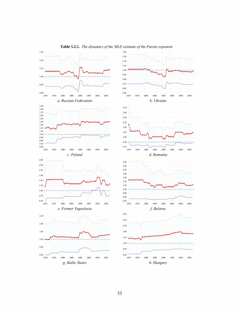
33

Table 5.2.1. The dynamics of the MLE estimate of the Pareto exponent

0.80

0.90

1.00

1.10

1.20

1.30

1970 1975 1980 1985 1990 1995 2000 20050.50

0.60

0.70

0.80

0.90

1.00

1.10

1.20

1.30

1.40

1970 1975 1980 1985 1990 1995 2000 2005

a. Russian Federation b. Ukraine

0.600.70

0.800.90

1.001.101.20

1.301.401.50

1.601.70

1.801.90

1970 1975 1980 1985 1990 1995 2000 20050.70

1.00

1.30

1.60

1.90

2.20

2.50

2.80

3.10

1970 1975 1980 1985 1990 1995 2000 2005

c. Poland d. Romania

0.40

0.70

1.00

1.30

1.60

1.90

2.20

2.50

2.80

1970 1975 1980 1985 1990 1995 2000 20050.40

0.60

0.80

1.00

1.20

1.40

1.60

1.80

2.00

2.20

2.40

1970 1975 1980 1985 1990 1995 2000 2005

e. Former Yugoslavia f. Belarus

0.20

0.60

1.00

1.40

1.80

2.20

1970 1975 1980 1985 1990 1995 2000 20050.20

0.60

1.00

1.40

1.80

2.20

2.60

3.00

1970 1975 1980 1985 1990 1995 2000 2005

g. Baltic States h. Hungary

34

0.20

0.60

1.00

1.40

1.80

2.20

2.60

1970 1975 1980 1985 1990 1995 2000 20050.00

0.50

1.00

1.50

2.00

2.50

1970 1975 1980 1985 1990 1995 2000 2005

i. Former Czechoslovakia j. Bulgaria

For the large majority of countries and time periods the estimated coefficient is

higher than one. However, as it is easily observable from Figure 5.2.1, one can not reject

that the Pareto exponent is significantly different from one, and therefore it seems that the

Zipf Law holds. This is in line with other studies in the literature that obtained favorable

evidence of Zipf’s Law in the upper-tail distribution of cities. On the other hand, we have

to be skeptical of the results since we employed asymptotic standard errors and the

sample sizes for some of the countries are rather reduced. The analysis can be improved

by computing standard errors using bootstrapping techniques, which are expected to

provide more robust results. Also, it is essential to obtain better standard errors since they

are employed in quantifying the consensus estimate of the Pareto exponent.

In the next section we employ detailed data to determine the distribution of city

size using different concurrent parametric models. Levy (2009) points out that, while the

lognormal distribution fits the empirical data extremely well for 99.4 percent of the size

range, as argued by Eeckhout (2004), in the top 0.6 percent range of the largest cities, the

size distribution diverges dramatically and systematically from the lognormal

distribution, and instead is much better described by a power law. Also, as pointed out by

Eeckhout (2009), a log-normal distribution of the tails does not mean that a Pareto fit

does not exist.

5.3 Results concerning the non-Pareto behavior of the city size distribution

In this section of the paper we present wide-scale comparisons of the estimates of

city size distribution obtained using power laws, the Weber-Fechner Law, and the

logarithmic hierarchy model as described in section 4.3.

35

We consider the development of cities in Kazakhstan, Uzbekistan, Kyrgyzstan,

Tajikistan and Turkmenistan that represent the so-called Central Asia region of the CIS 1.

Armenia, Azerbaijan and Georgia representing the so-called CIS Caucasus.

Since Zipf's Law with α≈1 holds only for the tails of distributions of cities that

include only large cities plus one or more mega-cities which contrast sharply in size to

the other cities, we will examine the occurrence of the Weber-Fechner Law in relation to

the size of cities and their rank. While Zipf's Law corresponds to a log-log relationship

between the ranks of large cities and their sizes

SizecRank loglog α−=

with the regression coefficient α equal to 1, the Weber-Fechner Law has the form

RankSize ⋅−= γβlog .

That is, in the case of the Weber-Fechner law, the rank of the city changes in

arithmetic progression with the change of the size of the city in geometric progression. In

this context one of our research objectives is to compare Weber’s constants γ for the

distribution of cities in different countries. Such comparisons will be further used to

describe the differences of urbanization processes in different countries and the impact of

administrative measures aimed at restricting the size of the capitals and large cities in

post-Soviet countries like Russia, Belarus, Central Asian countries and Caucasus

countries. This analysis is essential for any attempts to forecast the development of

urbanization in different countries.

While Zipf's Law is inherent to the communities, the Weber-Fechner Law is

typical for living organisms. The Weber-Fechner Law says: «The perception will grow in

arithmetic progression, when stimuli grow in geometric progression». This Law was

published in G. Fehner’s book “Elements of Psychophysics” in 1859. The Law was

discovered in the early 19th century by E. Weber a German physiologist and psychologist.

He studied in detail the link between perception and stimuli when he determined how to

1 At the summit of Central Asian states held in 1992, the President of Kazakhstan Nursultan Nazarbayev proposed to give up the term "Central Asia and Kazakhstan" in favor of the concept of "Central Asia" that covers all post-Soviet states in the region.

36

change a stimulus for this change to be noticed by a person. It turned out that a ratio of

stimulus change (intense) to its initial value is constant:

kII=

Δ ,

where I is the stimulus measure, ∆I is the stimulus change/intense, and k is Weber’s

constant.

Let i=1, …, n, be the rank of cities and towns in consideration. Let us interpret the

rank of cities/towns as a measure of perception that changes on an arithmetic progression

with a step (a difference) equal to 1. Let us also interpret the size of a city/town Ni (the

number of inhabitants) as the measure of a stimulus, since ranking has been made

according to this parameter. Denote by ∆Ni = Ni − Ni-1 , i=2,…, n, the change in the

stimulus. Let us suppose that

kNN

i

i =Δ

=const.

Changing ∆Ni by differential dNi, we have

kNdN

dNi

i

i == ln =const.

Solving the above differential equation, we obtain

ln Ni =c+k·i,

where c and k are some constants. Hence,

Ni =Aqi,

where A=ec, q=ek. In the sequel we will interpret q as the denominator of

geometric progression, that corresponds to the change in the “stimulus” Ni .

5.3.1. Zipf's Law

The following are the estimation results for the log-log rank-size regression with

the optimal shift 1/2 for Russia, Belarus, Central Asian and Caucasus cities. That is, the

estimated regression is

ln(i-1/2)= a - ζ⋅ln Ni,

37

where are the ordered city sizes in the samples considered

and i denotes the rank of i-th city.

Russia

Based on the number of urban dwellers in Rusia in 1897-2009, we estimated

regression coefficients ln(i-1/2)= a - ζ⋅lnNi, where Ni - size city (population size), i - rank

of the cities. The results are presented in Table A.5.3.1 in the Appendix.

Figure 5.3.1. Russian cities in 1897-2009 (the log-log scale)

Table 5.3.1. 95% confidence interval for coefficient ζ·of largest cities in Russia (with the population above 100 thousand people)

Years Sample size n

Estimated coefficient

ζ·

Standard error of the

estimation.2

95% confidence interval for the coefficient ζ·

1897 8 0.82414 0.41207 (0.016, 1.632) 1926 20 1.11359 0.352148 (0.423, 1.804) 1939 51 1.27545 0.252577 (0.780, 1.771) 1959 66 1.3038 0.226962 (0.859, 1.749) 1970 75 1.29735 0.211856 (0.882, 1.713) 1979 138 1.26617 0.152429 (0.967, 1.565) 1989 151 1.23767 0.14244 (0.958, 1.517)

2 Standard error of coefficient ζ is calculated according to the formula ζ

n2

.

38

2002 159 1.22786 0.13771 (0.958, 1.498) 2003 159 1.22668 0.137578 (0.957, 1.496) 2004 159 1.22984 0.137932 (0.959, 1.500) 2005 163 1.23317 0.136598 (0.965, 1.501) 2006 163 1.23459 0.136755 (0.967, 1.503) 2007 163 1.23494 0.136794 (0.967, 1.503) 2008 163 1.23463 0.13676 (0.967, 1.503) 2009 164 1.23284 0.136144 (0.966, 1.500)

According to the estimation results in Table 5.3.1, the confidence intervals for all

the samples considered contain the threshold value ζ=1 that corresponds to the Zipf's law.

Conclusion: Zipf's Law holds for the cities of the Russia.

Belarus

Based on the number of urban dwellers in Belarus in 1970-2009, we estimated

regression coefficients. The results are presented in Table 5.3.2.

Table 5.3.2. 95% confidence interval for coefficient ζ·of cities in Belarus

Years Sample size

Truncation, % n

Estimated coefficient

ζ·

Standard error of the estimation

S.e.= ζ)

n2

95% confidence interval for

ζ·

1970 198 20 41 1.038122 0.229 (0.589, 1.488)10 21 0.879841 0.272 (0.348, 1.412)

1979 200 20 41 1.056392 0.233 (0.599, 1.514)10 21 0.882730 0.272 (0.349, 1.417)

1989 202 20 41 1.050578 0.232 (0.596, 1.505)10 21 0.872941 0.269 (0.345, 1.401)

1990 202 20 41 1.044586 0.231 (0.592, 1.497)10 21 0.870052 0.269 (0.344, 1.396)

1991 202 20 41 1.036595 0.229 (0.588, 1.485)10 21 0.858082 0.265 (0.339, 1.377)

1992 202 20 41 1.040826 0.230 (0.590, 1.491)10 21 0.865029 0.267 (0.342, 1.388)

1993 202 20 41 1.037825 0.229 (0.589, 1.487)10 21 0.861267 0.266 (0.340, 1.382)

1994 202 20 41 1.033694 0.228 (0.586, 1.481)10 21 0.856657 0.264 (0.338, 1.375)

39

1995 202 20 41 1.031961 0.228 (0.585, 1.479)10 21 0.852876 0.263 (0.337, 1.369)

1997 203 20 41 1.022432 0.226 (0.580, 1.465)10 21 0.852783 0.263 (0.337, 1.369)

1998 205 20 41 1.036009 0.229 (0.588, 1.484)10 21 0.855515 0.264 (0.338, 1.373)

1999 205 20 41 1.034578 0.229 (0.587, 1.482)10 21 0.844820 0.261 (0.334, 1.356)

2000 205 20 41 1.034670 0.229 (0.587, 1.483)10 21 0.845432 0.261 (0.334, 1.357)

2001 207 20 41 1.035923 0.229 (0.587, 1.484)10 21 0.848378 0.262 (0.335, 1.362)

2002 207 20 41 1.038229 0.229 (0.589, 1.488)10 21 0.851213 0.263 (0.336, 1.366)

2003 206 20 41 1.041158 0.230 (0.590, 1.492)10 21 0.854345 0.264 (0.338, 1.371)

2004 206 20 41 1.044055 0.231 (0.592, 1.496)10 21 0.857012 0.264 (0.339, 1.375)

2005 206 20 41 1.047367 0.231 (0.594, 1.501)10 21 0.861484 0.266 (0.340, 1.383)

2006 206 20 41 1.049916 0.232 (0.595, 1.504)10 21 0.864966 0.267 (0.342, 1.388)

2007 207 20 41 1.052351 0.232 (0.597, 1.508)10 21 0.867555 0.268 (0.343, 1.392)

2008 206 20 41 1.056118 0.233 (0.599, 1.513)10 21 0.871507 0.269 (0.344, 1.399)

2009 206 20 41 1.059402 0.234 (0.601, 1.518)10 21 0.874751 0.270 (0.346, 1.404)

According to the estimation results in Table 5.3.2, the confidence intervals for all

the samples considered contain the threshold value ζ=1 that corresponds to the Zipf's law.

Conclusion: Zipf's Law holds for the cities of the Belarus.

Central Asia

Based on the number of urban dwellers in Central Asian countries in 1999, we

estimated regression coefficients3. The results are presented in Table 5.3.3.

Figure 5.3.2. Central Asian cities in 1999 (the log-log scale).

3 In 1999, the intersection data of all the countries of Central Asia.

40

Table 5.3.3. Estimates of the tail index ζ ( City sizes greater than 100 thousand people, data for 1999)

Country Number of

cities, m

Estimated tail index,

Standard errors,

95% confidence intervals for the tail

index ζ· Kazakhstan 19 1.646905 0.534327 (0.600, 2.694) Uzbekistan 17 1.266066 0.434257 (0.415, 2.117) Kyrgyzstan 2 0.857973 0.857973 (-0.824, 2.540) Tajikistan 2 0.827545 0.827545 (-0.794, 2.450) Turkmenistan 5 1.258920 0.796211 (-0.302, 2.819) Central Asia 45 1.491596 0.314456 (0.875, 2.108)

According to the estimation results in Table 5.3.3, the confidence intervals for all

the samples considered contain the threshold value ζ=1 that corresponds to the Zipf's law.

Conclusion: Zipf's Law holds for the cities of the Central Asia.

Caucasus

Based on the number of urban dwellers in countries of the Caucasus in 2007, we

estimated regression coefficients4. The results are presented in Table 5.3.4.

4 In 2007, the intersection data of all the countries of Caucasus.

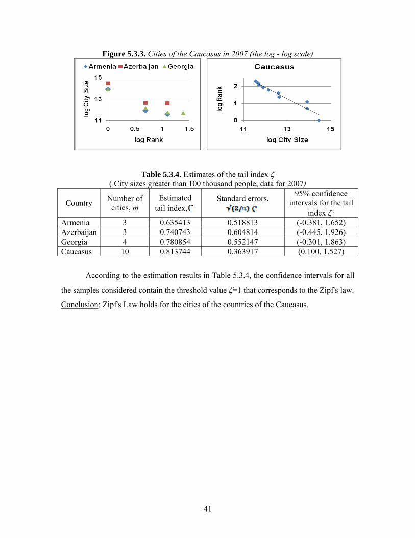
41

Figure 5.3.3. Cities of the Caucasus in 2007 (the log - log scale)

Table 5.3.4. Estimates of the tail index ζ ( City sizes greater than 100 thousand people, data for 2007)

Country Number of cities, m

Estimated tail index,

Standard errors,

95% confidence intervals for the tail

index ζ· Armenia 3 0.635413 0.518813 (-0.381, 1.652) Azerbaijan 3 0.740743 0.604814 (-0.445, 1.926) Georgia 4 0.780854 0.552147 (-0.301, 1.863) Caucasus 10 0.813744 0.363917 (0.100, 1.527)

According to the estimation results in Table 5.3.4, the confidence intervals for all

the samples considered contain the threshold value ζ=1 that corresponds to the Zipf's law.

Conclusion: Zipf's Law holds for the cities of the countries of the Caucasus.

42

5.3.2. Weber-Fechner Law

Russia

Estimates of the coefficients of regression ln Ni =c+k·i based on the data on the

population of the Russian cities for the years 1897-2009 as well as the coefficients of the

equation Ni =Aqi are given in table A5.3.2 in the Appendix and Table 5.3.5.

Table 5.3.5. Parameters of regression of logarithms of the population Ni for cities of Russia agaist its ranks: ln Ni =c+k·i, Ni =Aqi, where A=ec, q=ek (except for Moscow and

Saint-Petersburg) Years t c k A q r=1/q 1897 7 5.078591 -0.04017 160.5477 0.960631 1.040983 1926 36 5.819091 -0.04973 336.6659 0.951491 1.050982 1939 49 6.46233 -0.04125 640.5518 0.959585 1.042117 1959 69 6.801082 -0.03611 898.8193 0.964534 1.03677 1970 80 6.959886 -0.0303 1053.513 0.970157 1.030761 1979 89 6.71537 -0.01641 824.989 0.983729 1.01654 1989 99 6.823465 -0.01585 919.1644 0.984278 1.015973 2002 112 6.761217 -0.01502 863.6927 0.98509 1.015135 2003 113 6.757072 -0.01496 860.1201 0.985147 1.015077 2004 114 6.755904 -0.01497 859.116 0.985139 1.015086 2005 115 6.736914 -0.01457 842.9554 0.985534 1.014679 2006 116 6.736782 -0.01455 842.8441 0.985552 1.014659 2007 117 6.733465 -0.01455 840.053 0.98556 1.014651 2008 118 6.733453 -0.01455 840.0429 0.985558 1.014653 2009 119 6.734632 -0.01455 841.0339 0.98556 1.014651

In summary, the following conclusions can be made:

1. Development of cities of Russia can be well explained by the Weber-Fechner Law

(see table A5.3.2 in the Appendix).

2. Weber constant from the year 2006 has been equal to 0.01455.

3. For the change in the population to be noticeable (for infrastructure,

administrative decisions) this change should be greater than 1.5% of the

population of the city (r=1/q=1.015). Therefore, the decisions (administrative,

economic, ecological etc.) should be changed if the population of the cities

increases by more than 1.5%.

43

4. Moscow and Saint-Petersburg have the special status and do not comply with the

Weber-Fechner Law. Therefore, while forecasting the results of urbanization

Moscow and Saint-Petersburg should be given in the separate column, that is

independent on the decisions, adopted for other cities.

Change in the Weber coefficients

Curves regresionnyh dependencies ln Ni = c+k·i, the corresponding parameters

from Table 5.3.5, are shown in Figure 5.3.4.

Figure 5.3.4. Regressions ln Ni = c+k·i for Russian cities in 1897-2009

In Table A5.3.3 in the Appendix provides the estimation results for the regression

of the (estimated) parameters c and k on the time trend (the ranks t of years 1897, 1898,

..., 2009 and the dummy political variables P1, P2, P3 (P1 takes the value 0 before the

Great October Revolution and the value 1 after the revolution, P2 takes the value 0 before

the Second World War and a value of 1 after the Second World War, P3 takes the value 0

to the collapse of the USSR and the value 1 after the collapse of the USSR).

Acceptable from the standpoint of the Statistical significance of regression

coefficients and the model as a whole, the model interaction are 2, 3 and 4 for the

parameter c (all coefficients are significant with a probability of error less than 0.09). For

the parameter k as all coefficients are significant with a probability of error of no more

than 0.09.

Thus, there is

1. 263006.0106212.1078591.5 PPc ⋅+⋅+= ,

44

2. 3687989.0019399.047273.31 Ptc ⋅−⋅+−= ,

3. 3164946.0257245.01966226.0002678.0 PPPtc ⋅−⋅+⋅+⋅= ,

3011622.02008002.01029829.000069.0349853.1 PPPtk ⋅−⋅−⋅−⋅+−= ,

1. ))3011622.02008002.01029829.000069.0349853.1exp((

)263006.0106212.1078591.5exp(iPPPt

PPNi

⋅⋅−⋅−⋅−⋅+−⋅⋅⋅+⋅+=

2. ))3011622.02008002.01029829.000069.0349853.1exp((

)3687989.0019399.047273.31exp(iPPPt

PtNi

⋅⋅−⋅−⋅−⋅+−⋅⋅⋅−⋅+−=

3. ))3011622.02008002.01029829.000069.0349853.1exp((

)3164946.0257245.01966226.0002678.0exp(iPPPt

PPPtNi

⋅⋅−⋅−⋅−⋅+−⋅⋅⋅−⋅+⋅+⋅=

that is ii PtqPtAN ),(),( ⋅= , where

1. )263006.0106212.1078591.5exp(),( PPPtA ⋅+⋅+= ,

2. )3687989.0019399.047273.31exp(),( PtPtA ⋅−⋅+−=

3. )3164946.0257245.01966226.0002678.0exp(),( PPPtPtA ⋅−⋅+⋅+⋅=

)3011622.02008002.01029829.000069.0349853.1exp(),( PPPtPtq ⋅−⋅−⋅−⋅+−= .

Thus, the Great October Revolution and the Second World War gave the effect of

increasing the size of the largest cities of Russia and the Soviet collapse gave the effect of

reducing the size (ceteris paribus)

Belarus

Estimates of the coefficients of regression ln Ni =c+k·i based on the data on the

population of the Belarusian cities for the years 1970-2009 as well as the coefficients of

the equation Ni =Aqi are given in tables A5.3.4, A.5.3.5 in the Appendix and Table 5.3.6.

45

Table 5.3.6. Parameters of regression of logarithms of the population Ni for cities of Belarus agaist its ranks: ln Ni =c+k·i, Ni =Aqi, where A=ec, q=ek.

Year c k A q r=1/q

1970 3.656932 -0.018014 38.742 0.9821 1.0182 1979 4.017004 -0.019605 55.534 0.9806 1.0198 1989 4.333892 -0.02099 76.240 0.9792 1.0212 1990 4.366013 -0.021041 78.729 0.9792 1.0213 1991 4.382248 -0.021133 80.018 0.9791 1.0214 1992 4.398832 -0.021238 81.356 0.9790 1.0215 1993 4.416907 -0.021356 82.840 0.9789 1.0216 1994 4.432715 -0.021437 84.160 0.9788 1.0217 1995 4.437681 -0.021431 84.579 0.9788 1.0217 1997 4.457189 -0.021565 86.245 0.9787 1.0218 1998 4.43477 -0.021255 84.333 0.9790 1.0215 1999 4.423677 -0.021485 83.402 0.9787 1.0217 2000 4.428232 -0.021539 83.783 0.9787 1.0218 2001 4.414205 -0.021282 82.616 0.9789 1.0215 2002 4.416414 -0.021354 82.799 0.9789 1.0216 2003 4.41247 -0.021361 82.473 0.9789 1.0216 2004 4.409145 -0.021384 82.199 0.9788 1.0216 2005 4.410506 -0.021489 82.311 0.9787 1.0217 2006 4.41131 -0.021573 82.377 0.9787 1.0218 2007 4.414477 -0.02166 82.639 0.9786 1.0219 2008 4.416968 -0.021725 82.845 0.9785 1.0220 2009 4.421704 -0.021776 83.238 0.9785 1.0220

In summary, the following conclusions can be made:

1. Development of cities of Belarus can be well explained by the Weber-Fechner

Law (see table A5.3.4 in the Appendix).

2. Weber constant from the year 2006 has been equal to 0.022.

3. For the change in the population to be noticeable (for infrastructure,

administrative decisions) this change should be greater than 2.2% of the

population of the city (r=1/q=1.022). Therefore, the decisions (administrative,

economic, ecological etc.) should be changed if the population of the cities

increases by more than 2.2%.

46

Change in the Weber coefficients

Curves regresionnyh dependencies ln Ni = c+k·i,, the corresponding parameters

from Table 5.3.6, are shown in Figures 5.3.5, 5.3.6.

Figure 5.3.5. Change of parameters a of the Weber-Fechner Model Rank=c+klnSize with 1970 for 2009 for settlements of Belarus

Figure 5.3.6. Change of parameters k of the Weber-Fechner Model Rank=c+klnSize with 1970 for 2009 for settlements of Belarus

Calculations show that the collapse of the Soviet Union at the rate of urban

growth in the Belarus statistically significant effects are not influence.

47

Central Asia

Estimates of the coefficients of regression ln Ni =c+k·i based on the data on the

population of the Central Asia cities for the year 1999 as well as the coefficients of the

equation Ni =Aqi are given in tables A5.3.6 in the Appendix and Table 5.3.7.

Table 5.3.7. Parameters of regression of logarithms of the population Ni for cities of Central Asia in 1999 agaist its ranks: ln Ni =c+k·i, Ni =Aqi, where A=ec, q=ek.

Number of cities c k A q r=1/q 45 13.36066 -0.045002 634542.788 0.955996 1.04602995

In summary, the following conclusions can be made:

1. Development of cities of Central Asia can be well explained by the Weber-

Fechner Law (see table A5.3.6 in the Appendix).

2. Weber constant is equal to 0.045.

3. For the change in the population to be noticeable (for infrastructure,

administrative decisions) this change should be greater than 4.6% of the

population of the city (r=1/q=1.046). Therefore, the decisions (administrative,

economic, ecological etc.) should be changed if the population of the cities

increases by more than 4.6%.

Change in the Weber coefficients

Estimates of the coefficients of regression ln Ni =c+k·i based on the data on the

population of the Central Asian cities for the years 1970-2006 as well as the coefficients

c and k are given in tables A5.3.7 in the Appendix and Table 5.3.8.

Table 5.3.8. Parameters of regression of logarithms of the population Ni for cities of Central Asia agaist its ranks: ln Ni =c+k·i.

Years c k 1970 13.21387 -0.06884 1971 13.24355 -0.06884 1975 13.30165 -0.06317 1980 13.32473 -0.05399 1985 13.39433 -0.052 1987 13.40747 -0.04943 1990 13.41749 -0.05069 1999 13.36066 -0.045 2006 13.48998 -0.05169

48

The following Figure 5.3.7 illustrates the regressions ln Ni = c+k·i estimated in Table

5.3.8.

Figure 5.3.7. Regressions ln Ni = c+k·i for Central Asian cities in 1970-2006

Figure 5.3.8. Weber relations Ni =Aqi for Central Asian cities in 1970-2006

Table A5.3.8 in the Appendix provides the estimation results for the regression of the

(estimated) parameters c and k on the time trend (the ranks t of years 1970, 1971, ...,

2006) and the dummy political variable P that takes value 0 prior to the collapse of the

USSR in 1991 and value 1 afterwards.

49

Thus, the estimated regressions are

Ptc ⋅−⋅+−= 144598.0010573.0601766.7 ,

Ptk ⋅−⋅+−= 011148.0000919.0877394.1 ,

iPtPtNi ⋅⋅−⋅+−+⋅−⋅+−= )011148.0000919.0877394.1(144598.0010573.0601766.7ln,

))011148.0000919.0877394.1exp(()144598.0010573.0601766.7exp( iPtPtNi ⋅⋅−⋅+−⋅⋅−⋅+−=

that is ii PtqPtAN ),(),( ⋅= , where )144598.0010573.0601766.7exp(),( PtPtA ⋅−⋅+−= ,

)011148.0000919.0877394.1exp(),( PtPtq ⋅−⋅+−= .

Consequently, the disintegration of the USSR led to a decrease in the growth of

cities in Central Asia. Apparently this is due to the emigration of non-indigenous people

in other countries.

Caucaus

Estimates of the coefficients of regression ln Ni =c+k·i based on the data on the

population of the Caucasus cities for the year 2007 as well as the coefficients of the

equation Ni =Aqi are given in tables A5.3.9 in the Appendix and Table 5.3.9.

Table 5.3.9. Estimates for the regression ln Ni =c+k·i and the implied relation Ni =Aqi

for cities of Caucasus Asia in 2007 Number of cities c k A q r=1/q

10 14.50335 -0.336194 1989412.65 0.714484 1.39961052

In summary, the following conclusions can be made:

1. Development of cities of Caucasus can be explained by the Weber-Fechner Law

(see Table A5.3.9 in the Appendix).

2. The Weber constant is equal to 0.336.

3. For the change in the population to be noticeable (for infrastructure,

administrative decisions) this change should be greater than 39.96≈40% of the

population of the city (r=1/q=1.39961). Therefore, the decisions (administrative,

50

economic, ecological etc.) should be changed if the population of the cities

increases by more than 40%.

Changes in the Weber coefficients

Estimates of the coefficients of regression ln Ni =c+k·i based on the data on the

population of the Caucasus cities for the years 1970-2007 as well as the coefficients of

the equation Ni =Aqi are given in tables A5.3.10 in the Appendix and Table 5.3.10.

Table 5.3.10. Estimates of the parameters c and k in the regression ln Ni = c+k·i for the

cities in the Caucasus in 1970-2007 Years c k 1970 13.86252 -0.276535 1971 13.88072 -0.274877 1975 13.98215 -0.257304 1980 14.12501 -0.2618 1985 14.21326 -0.26222 1987 14.24711 -0.262647 1990 14.29858 -0.299119 2007 14.50335 -0.336194

Figure 5.3.9. Parameters c and k of regression ln Ni = c+k·i for cities of Caucasus in

1970-2007

Table A5.3.11 in the Appendix provides the estimation results for the regression

of the (estimated) parameters c and k on the time trend (the ranks t of years 1970, 1971,

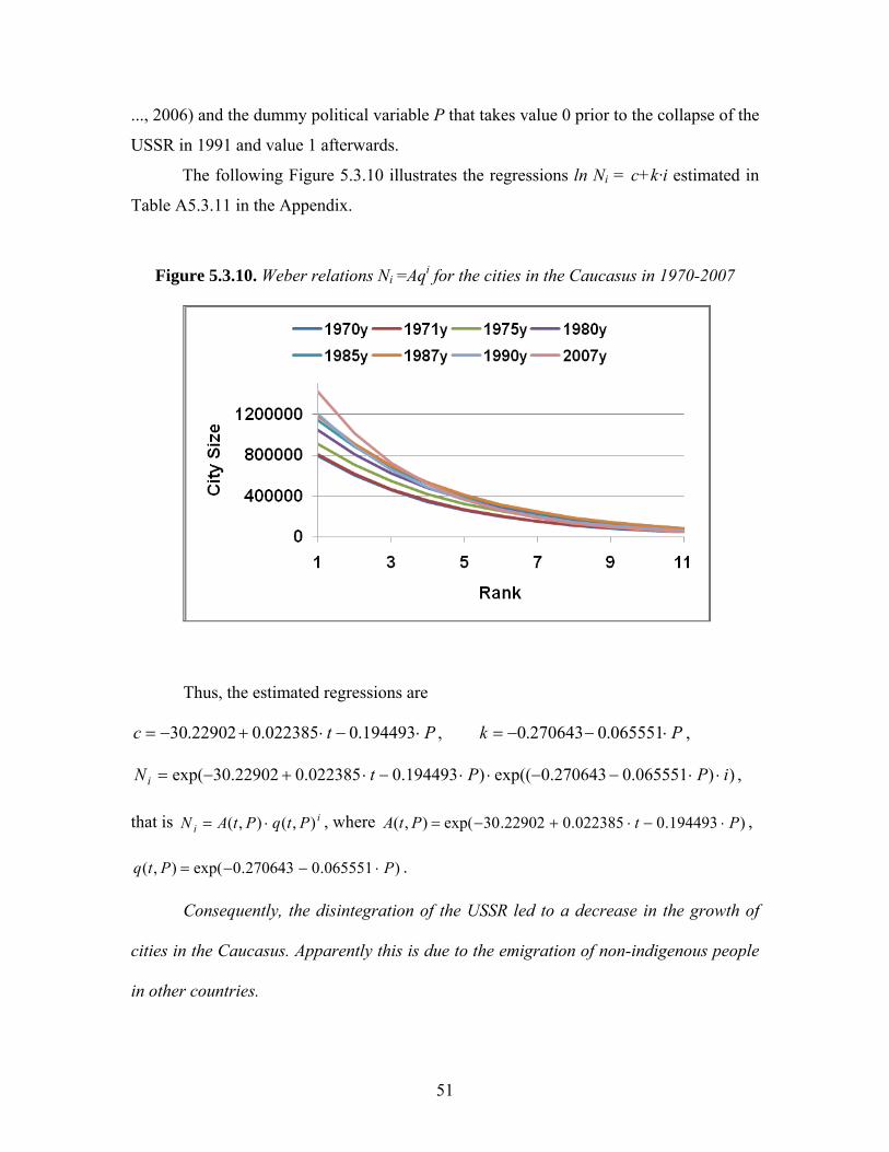
51

..., 2006) and the dummy political variable P that takes value 0 prior to the collapse of the

USSR in 1991 and value 1 afterwards.

The following Figure 5.3.10 illustrates the regressions ln Ni = c+k·i estimated in

Table A5.3.11 in the Appendix.

Figure 5.3.10. Weber relations Ni =Aqi for the cities in the Caucasus in 1970-2007

Thus, the estimated regressions are

Ptc ⋅−⋅+−= 194493.0022385.022902.30 , Pk ⋅−−= 065551.0270643.0 ,

))065551.0270643.0exp(()194493.0022385.022902.30exp( iPPtNi ⋅⋅−−⋅⋅−⋅+−= ,

that is ii PtqPtAN ),(),( ⋅= , where )194493.0022385.022902.30exp(),( PtPtA ⋅−⋅+−= ,

)065551.0270643.0exp(),( PPtq ⋅−−= .

Consequently, the disintegration of the USSR led to a decrease in the growth of

cities in the Caucasus. Apparently this is due to the emigration of non-indigenous people

in other countries.

52

5.3.3. Hierarchy of logarithms

Though communication of type of Weber-Fechner between quantity of inhabitants

of cities and their ranks is comprehensible from the point of view of the statistical

importance, specification of a kind of dependence is desirable. It has appeared possible to

be made by means of hierarchy of logarithms in the regress equation.

Ruissia

We will designate: ln4 (⋅)=ln(ln(ln(ln(⋅)))). In Figure 5.3.11 sites of cities of Russia

on a scale are resulted “Rank - ln4(Population)“.

Figure 5.3.11. Russian cities in 1897-2009 (Except for Moscow and Saint-Petersburg)

Table 5.3.11. Estimates of the parameters c and k in the regression ln4 Ni = c4+ k4·i for the cities in Russia in 1897-2007

Yeares c4 k4

1897 -0.163 -0.04339 1926 -0.43223 -0.01968 1939 -0.31021 -0.01384 1959 -0.28938 -0.01074 1970 -0.35158 -0.00642

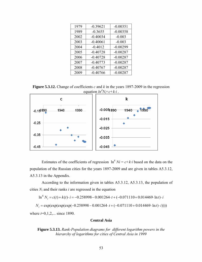
53

1979 -0.39621 -0.00351 1989 -0.3655 -0.00358 2002 -0.40034 -0.003 2003 -0.40061 -0.003 2004 -0.4012 -0.00299 2005 -0.40728 -0.00287 2006 -0.40728 -0.00287 2007 -0.40773 -0.00287 2008 -0.40767 -0.00287 2009 -0.40766 -0.00287

Figure 5.3.12. Change of coefficients c and k in the years 1897-2009 in the regression equation ln4Ni=c+k⋅i .

Estimates of the coefficients of regression ln4 Ni = c+k·i based on the data on the

population of the Russian cities for the years 1897-2009 and are given in tables A5.3.12,

A5.3.13 in the Appendix.

According to the information given in tables A5.3.12, A5.3.13, the population of

cities Ni and their ranks i are regressed in the equation

ittitktcNi ⋅⋅+−+⋅−−=⋅+= )ln014469.0071110.0(001264.0258998.0)()(ln4

)))))ln014469.0071110.0(001264.0258998.0p(exp(exp(exp(ex ittNi ⋅⋅+−+⋅−−=

where t=0,1,2,... since 1890.

Central Asia

Figure 5.3.13. Rank-Population diagrams for different logarithm powers in the hierarchy of logarithms for cities of Central Asia in 1999

54

Note. (II) – ln2(Ni), (III) - ln3(Ni), (IV) - ln4(Ni), where )(ln ⋅r means the r-th iterations of logarithms. Estimates of the coefficients of regression lnr Ni = c+k·i based on the data on the

population of the Central Asian cities in 1999 and are given in table A5.3.14 in the

Appendix.

According to Table А5.3.14 the best in all respects is the model

iN i ⋅−−= 001534.0048076.0)(ln 4 ,

))))001534.0048076.0p(exp(exp(exp(ex iNi ⋅−−= . (5.3.1)

This model describes well the distribution of all cities in Central Asia except the three

outliers of Tashkent, Almaty and Bishkek (see Figure 5.3.14).

Figure 5.3.14. The distribution of cities in Central Asia in 1999 and fitted model (5.3.1)

55

Caucasus

Figure 5.3.15. Rank-Population diagrams for different logarithm powers in the hierarchy of logarithms for the cities of the Caucasus in 2007

Note. (II) – ln2(Ni), (III) - ln3(Ni), (IV) - ln4(Ni), где )(ln ⋅r means r iterations of logarithms. Estimates of the coefficients of regression lnr Ni = c+k·i based on the data on the

population of the Caucasus cities in 2007 and are given in table A5.3.15 in the Appendix.

According to Table А5.3.15 the best in all respects is the model

iN i ⋅−−= 010991.0013023.0)(ln 4 ,

))))010991.0013023.0p(exp(exp(exp(ex iNi ⋅−−= . (5.3.2)

This model describes well the distribution of all cities in Central Asia except the

outlier of Baku (see Figure 5.3.16).

Figure 5.3.16. The distribution of cities in the Caucasus by rank in 2007 and fitted model

(5.3.2)

56

Therefore we can conclude that:

1. The distribution of the size of the largest cities of Russia, Belarus, Central

Asia and Caucasus is consistent with Zipf's law.

2. The distribution of the size of the size (all) cities of Russia, Belarus, Central

Asia and Caucasus satisfies the law of Weber-Fechner except the largest

Megapolyus.

3. The Great October Revolution and World War II led to an increase in Russian

cities due to influx of rural population in the city. When Stalin began forced

urbanization, people from villages in the 30 th, 40 th, 50 th years, went into

the city.

4. The collapse of the USSR led to a relative reduction cities of Central Asia and

Caucasus as a result of relocation of non-indigenous population in rural areas

of Russia. The collapse of the USSR at the rate of urban growth in the Belarus

statistically significant effects are not influence.

5. Distribution of cities in Russia, Belarus, Central Asia and Caucasus is best

described by models based on the hierarchy of the logarithms of their sizes.

5.4 Results concerning the “within distribution” city dynamics

5.4.1 Markov chains analysis

In this section, we apply Markov chains analysis to study a movement speed and

form of convergence within the city size distribution. We employ data on population of

all cities for Belarus, Hungary, Poland, and for 479 of Russia (out of 1037 cities

according to 2002 census). The dataset is described in Table A5.4.1 in the Appendix.

The main sources of the detailed city data are the national official statistical

information services of CEE and CIS countries. Data in national statistics are presented

for census years as well as estimates on the beginning of the corresponding year. The

number of cities and other characteristics of urban systems of Belarus, Hungary, Poland,

and Russia are described in the Table 5.4.1.

57

Table 5.4.1. The main description of the data by countries.

Indicator Belarus Poland 1970 1989 2009 1970 1989 2009

Number of cities 198 202 206 802 828 890

Urban pop. (ths) 3886.9 6768.5 7148.5 18492.7 23455.3 23279.4

Size of a min city 1.2 0.7 0.6 1 1.2 0.9

Average city size 19.6 33.5 34.7 23 28.3 26.2

Size of a max city 907.1 1612.8 1829.1 1387.8 1651.2 1709.8

Table 5.4.2. (continuation)

Indicator Hungary Russia 1970 1989 2001 1970 1989 2007

Number of cities 237 237 237 479 479 479

Urban pop. (ths) 6124.3 6741.1 6415.7 52971.1 69437.2 77927.7

Size of a min city 0.68 1.1 1.4 1.9 1.3 1.15

Average city size 25.8 28.4 27 110.6 145 197

Size of a max city 1945.1 1934.8 1712.7 7063 8769.1 10126.4

In order to carry out the methodology described in section 4.4, we should choose

a discretization of the cities’ sizes. As pointed out by Magrini (1999), an improper

discretization may have the effect of removing the Markov property and therefore may

lead to misleading results, especially as is in our case when computations of ergodic

distributions are based on the estimates of the discrete transition probabilities. Quah

(1993) and Le Gallo (2004) choose to discretize the distribution in such a way that the

initial classes include a similar number of elements. Cheshire and Magrini (2000) base

their choice between possible classes in terms of the ability of the discrete distribution to

approximate the observed continuous distribution.

58

In our study following the paper of Le Gallo and Chasco (2009), we have tried

different ways of discretizing the distribution, divided it on 5, 6 and 7 classes. We chose

Poland to check possible distributions providing we have the biggest dataset for this

country (890 cities) and this country is one of the most successful among transition

economies. Final discretization should be chosen by considering the best performance of

the test for order one for all countries’ city distributions.

The assumption of a first-order stationary Markov process requires the transition

probabilities, ijp , to be of order 1, that is, to be independent of classes at the beginning of

previous periods (at time t − 2, t − 3, …). If the chain is of a higher order, the first-order

transition matrix will be misspecified. Indeed, it will contain only part of the information

necessary to describe the true evolution of population distribution. Moreover, the Markov

property implicitly assumes that the transition probabilities, ijp , depend on i (i.e., that the

process is not of order 0).

In order to test this property, Bickenbach and Bode (2003) emphasize the role of

the test of time independence. In determining the order of a Markov chain, Tan and

Yilmaz (2002) suggest, firstly, to test order 0 versus order 1; secondly, to test order 1

versus order 2; and so on. If the test of order 0 against order 1 is rejected, and the test of

order 1 against order 2 is not rejected, the process may be assumed to be of order 1.

After trying different variants we decided to divide all cities on seven classes: 1)

population less than 10% of the countries’ average, 2) population between 10 and 20% of

the average 3) population between 20 and 30% of the average, 4) population between 30

and 50% of the average, 5) population between 50 and 100% of the average, 6)

population between 100 and 200% of the average, and 7) population more than 200% of

the average. This division appears to give relatively balanced distribution for all four

countries.

However the way of cities’ division on classes could be changed after considering

the performance of the test for Markovity of order one for all countries with detailed data.

We can get different results of that test for different countries and this will give us

information about a possibility to build more balanced classes at some cost to this test for

certain countries.

59

To test for order 0, the null hypothesis 0 : 1, , ij iH i K p p∀ = =K is tested against the following alternative : {1,..., }a ij jH i K p p∃ ∈ ≠ . The appropriate likelihood ratio (LR) test statistic reads as follows:

( )( (0)) 2 2

12 ( ) ln ( 1) ,

i

KijO

iji j A i

pLR n t K

pχ

= ∈

= −∑∑

assuming that 0ip > , {1,.., }i K∀ ∈ , { : 0}i ijA j p= > is the set of nonzero transition

probabilities under Ha

To test for order 1 versus 2, a second-order Markov chain is defined by also

taking into consideration the population size classes in which the cities were at time t − 2

and assuming that the pair of successive classes k and i forms a composite class. Then,

the probability of a city moving to class j at time t, given it was in k at t − 2 and in i at t −

1, is kijp . The corresponding absolute number of transitions is kijn , with the marginal

frequency being ( )1 ( 1)ki kijj

n t n t− = −∑ To test 0 : {1,..., } kij ijH k K p p∀ ∈ = against

: {1,..., }a kij ijH k K p p∃ ∈ ≠ , the kijkij

ki

np

n= , where

2( )

T

kij kijt

n n t=

=∑2

( 1)T

ki kit

n n t=

= −∑ . The

ijp are estimated from entire data set as ijij

i

np

n= . Appropriate LR test statistic reads as

follows:

( (1)) 2

1 1 1

2 ( ) ln ( 1)( 1) .hi

K K KkijO

k ij i ik i j C iij

pLR n t c d

pχ

= = ∈ =

⎛ ⎞= − −⎜ ⎟⎝ ⎠

∑∑ ∑ ∑

Similar to the notation above, { : 0},i ijC j p= > #i ic C= , { : 0},ki kijC j p= > and #{ : 0}i kid k n= > . In our case 7K = .

If both Markovity of order 0 and of order 1 are rejected, the tests can be extended

to higher orders by introducing additional dimensions for population size at time t − 3, t −

4, and so on. However, since the number of parameters to be estimated increases

exponentially with the number of time lags, while the number of available observations

decreases linearly for a given data set, the reliability of estimates and the power of the

test decrease rapidly. Therefore, Tan and Yilmaz (2002) suggest setting an a priori limit

up to which the order of the Markov chain can be tested.

60

All results of testing Markovity for every country one can observe in Appendix

Table A.5.4.2 – Table A.5.4.10. In our case most data passed the tests for Markovity of

order greater or equal to one.

For instance, see Table A.5.4.2. (Poland), Markovity of order 0 is tested using test

statistic (5.4.1) at every moment t= 1961, 1974, 1985, 1994, 2004 (in our investigations

parameter t runs by decades, or approximately by decades depending on lack of data on

some country). The result ( (0)) (1961) 1943.578OLR = , prob=0, df=36 leaves no doubt that

the process strongly depends on the initial condition at time t-1. That is the chain is at

least of order 1. Applying the test statistic (5.4.2.2) to the same moments of time we get

the result: ( (1)) (1964) 396.545OLR = − , prob=0, df=28 indicating about Markovity of order

1 and higher. As we mentioned above we cannot continue test of Marcovity order 1

versus 2 etc., because of exponential growth of parameters to be estimated with having

bounded data.

Received Markovity test results for all countries with detailed data mean that we

do not need to perform a revision of the discretization of cities on classes for Markov

chains estimation procedure.

Tables A.5.4.11. – A.5.4.14. contain the first-order transition probability matrices

with the ML estimates ijp of the transition probabilities for population in Poland,

Belarus, Hungary, and Russia.  

Note that all transition probability matrices for studying countries are regular.

Matrices let us draw conclusions on intensity of interclass movements. Using those

matrices according to methodology described, we can extract information related to

cities’ mobility speed and convergence pattern.

For example, in Poland during the half of a century, there were 459 instances of a

city having a population size lower than 10 percent of the average. The majority of these

cities (78.6%) remained in that size class at the end of the decade, while 15.5% moved up

one class by the end of the decade.

The high probabilities on the diagonal in all countries show a low interclass

mobility, i.e., a high-persistence of cities to stay in their own class from one observation

to another over the whole period. Eaton and Eckstein (1997) interpret diagonal elements

61

of the transition approaching 1 as parallel growth. Since these elements are not exactly 1,

we can analyze the propensity of cities in each cell to move into other cells. In particular,

it appears that the largest and smallest cities (classes 1 and 7, respectively) have higher

persistence while medium-sized cities (categories 3, 4 and 5) have more probability of

moving to smaller categories. In classes 2 and 3 a small number of cities if any move up

to higher categories more than two steps. Only in case of Poland in classes 2 and 3 the

probability of moving up a class exceeds that of moving down. In Belarus the probability

of moving down a class exceeds that one in other countries.

This low inter-class mobility of cities is in line with the results found for other

cases such as US MSA’s (Black and Henderson 2003) and all Spanish municipalities (Le

Gallo and Chasco 2009).

Then, in order to determine the speed with which the cities move within the

distribution, we consider the matrix of mean first passage time PM , where every element

indicates the expected time for a city to move from class i to class j for the first time

(Tables A.5.4.15 – A.5.4.2.18). PM is defined as (Kemeny and Snell 1976, Chap. 4):

( )P dgM I Z Z D= − +1

where I is the identity matrix, * 1( )Z I M M −= − + , M is the probability transition matrix, * lim n

nM M

→∞= , 1 is a matrix of ones, dgZ results from Z setting off-diagonal

entries to 0, and * *1

1 1,...,K

D Diagm m

⎧ ⎫= ⎨ ⎬

⎩ ⎭, * *

1 ,.., Km m are elements of *M .

For example, the expected time for Belarusian city to move from class 1 to class 2

is equal to 220 years, while the moving from 2 to 1 will happened in 99 years. In whole

the mean number of years to reach any class is relatively high: for example, the shortest

time passage for Poland is 115 years (move from class 1 to class 3) and the longest is

6060 years (move from class 7 to class 1). We should remember that these calculations

account for the fact that starting from class 4, a city might visit classes 6, 5, 3, 2 or 1

before going to class 7.

Belarusian matrix shows the passage from higher class to lower one is more

probable than from lower to higher. That is not the truth for Polish and Hungarian cities

where the moving to higher class is faster. For example, for Belarusian cities to first visit

62

class 7 from class 1 it takes 40077 years, while for Polish and Hungarian it takes 827 and

8168.8 years respectively. On the contrary, to first visit class 1 from class 7 it takes 1190

years for cities in Belarus, while for Poland and Hungary it takes 6060 and 2195 years

respectively. In Belarusian and Russian matrices all upper diagonal elements greater than

lower diagonal ones. That means Belarusian and Russian cities tends from higher class to

lower one. All upper diagonal elements of Polish matrix less that lower diagonal ones.

That is all Polish cities tend to move  from lower classes to higher ones. The situation

with Hungarian matrix is a bit different. We can see that more probable moves from

lower classes to higher ones take place up to third class (upper diagonal elements less

than lower ones). From fourth to seven classes we can see backward moves (upper

diagonal elements greater than lower ones). Comparing with results of Le Gallo and

Chasco (2009), obtained for Spanish urban system we may say that maximal entry of the

mean first passage matrix is 3110,7 years. It corresponds to a mean first time passage of a

city from first class to last (sixth) class. Moves happen more probably between neighbor

classes. Minimal time to move between classes is 91.9 years. It is a transition from class

5 to class 4.

The difference in the models of urban system development and the forms of

cities’ convergence for Belarus, Russia on the one part and Poland and Hungary on the

other part becomes obvious after comparison of initial versus ergodic distribution pattern

matching (Tables A.5.4.19. – A.5.4.22) or see Figure 5.4.1.

Figure 5.4. 1 Initial and ergodic distribution of cities’ sizes in Poland, Belarus, Hungary, and Russia

Initial Distribution (Poland)

-0.1

0.1

0.3

0.5

0.7

1 2 3 4 5 6 7Classes

Egrodic Distribution (Poland)

-0.1

0.1

0.3

0.5

0.7

1 2 3 4 5 6 7Classes

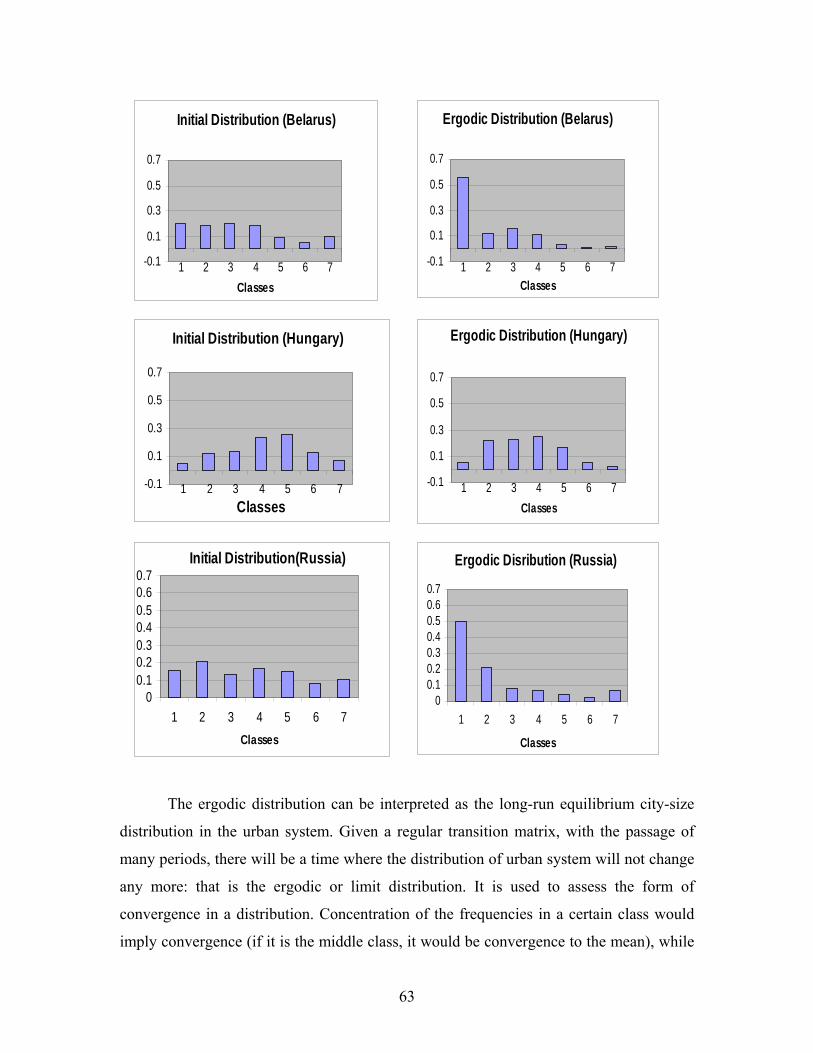
63

Initial Distribution (Belarus)

-0.1

0.1

0.3

0.5

0.7

1 2 3 4 5 6 7Classes

Ergodic Distribution (Belarus)

-0.1

0.1

0.3

0.5

0.7

1 2 3 4 5 6 7Classes

Initial Distribution (Hungary)

-0.1

0.1

0.3

0.5

0.7

1 2 3 4 5 6 7Classes

Ergodic Distribution (Hungary)

-0.1

0.1

0.3

0.5

0.7

1 2 3 4 5 6 7Classes

Initial Distribution(Russia)

00.10.20.30.40.50.60.7

1 2 3 4 5 6 7Classes

Ergodic Disribution (Russia)

00.10.20.30.40.50.60.7

1 2 3 4 5 6 7

Classes

The ergodic distribution can be interpreted as the long-run equilibrium city-size

distribution in the urban system. Given a regular transition matrix, with the passage of

many periods, there will be a time where the distribution of urban system will not change

any more: that is the ergodic or limit distribution. It is used to assess the form of

convergence in a distribution. Concentration of the frequencies in a certain class would

imply convergence (if it is the middle class, it would be convergence to the mean), while

64

concentration of the frequencies in some of the classes, that is, a multimodal limit

distribution, may be interpreted as a tendency towards stratification into different

convergence clubs. Finally, a dispersion of this distribution amongst all classes is

interpreted as divergence.

The results for Poland, Belarus, Hungary and Russia are reported on the

histograms of Figures 5.4.1., 5.4.2., A.5.4.1. and demonstrate significant differences

among countries. For Belarus and Russia it appears that the ergodic distribution is more

concentrated in the small and lower middle-size cities (1st to 4th classes), a result that

reveals the existence of convergence towards smaller size populations. For Poland it

appears that the ergodic distribution is more concentrated in the middle and big-size cities

(5th to 7th classes). At the same time, one can see that a level of stability of ergodic

distribution compared to the initial one for Belarus, Poland, and Russia is low, while it is

relatively more stable for Hungarian distribution. The Figure 5.4.2. shows quantitative

difference between ergodic and initial distributions. Figure 5.4.2. Difference between Initial and Ergodic distributions of cities’ sizes in Poland, Belarus,

Hungary, and Russia

Polish Distribution Difference

-0.3

-0.1

0.1

0.3

0.5

0.7

1 2 3 4 5 6 7

Belarusian Distribution Difference

-0.3

-0.1

0.1

0.3

0.5

0.7

1 2 3 4 5 6 7

Hungarian Distribution Difference

-0.3

-0.1

0.1

0.3

0.5

0.7

1 2 3 4 5 6 7

Russian Distribution Differences

-0.3

-0.1

0.1

0.3

0.5

0.7

1 2 3 4 5 6 7

65

As one can see Belarus and Russia evolves to the country of small cities, while

Poland and Hungary to the country of big and medium sized cities respectively. Studying 

probability transition matrices and mean first passage time matrices of investigated

countries we may say something about movements of cities within the distribution. In

case of Hungary probability (see Table A.5.4.13.) to pass from 1 class to 2 four times

bigger than from 2 to1, probability to pass from 3 class to 2 is greater than that from 2 to

3. That is cities from 1 and 3 class will move to second one. Furthermore, cities from 7

class will probable to move to 6, cities from 6 class more probable to move in 5 and so

on. 

Our results for initial and ergodic distributions are comparable with those for

Spanish municipalities obtained by Le Gallo and Chasco (2009). Their study shows

slightly downward convergence to the second and third classes and is similar to

Hungarian pattern.

It may be interesting to represent the differences in the forms of distributions in

numerical quantities. We may compare ergodic, initial distributions, and their difference

with help of kurtosis statistics: ( )

( )

4

12

2

1

( ) 3

n

ii

n

ii

n x XKurt X

x X

=

=

−= −⎛ ⎞

−⎜ ⎟⎝ ⎠

∑

∑,

that is close to zero if X close to symmetric Gaussian distribution, and far from zero

otherwise. The bigger kurtosis the more sharp the peak of X distribution. In terms of

shape, such distribution has a more acute peak around the mean (that is, a lower

probability than a normally distributed variable of values near the mean) and fatter tails

(that is, a higher probability than a normally distributed variable of extreme values). A

distribution with negative excess kurtosis is more "broad". In terms of shape, a such type

of distribution has a lower, wider peak around the mean (that is a curve of such

distribution is mostly convex upward) and thinner tails (that is a curve of such

distribution has a narrow domain where it is convex downward). Table A.5.4.24 depicts

values of the kurtosis across all countries and shows that Hungarian ergodic and initial

distributions are most balanced among all countries. Therefore, we propose to consider

Hungarian urban system distribution as a benchmark for assessment of deviations of

66

Belarusian, Russian and Polish ones. It is clear from the table that all countries initially

had low kurtosises. However, magnitudes of kurtosis for ergodic distributions changes

and we may arrange countries in order by growing urban pattern starting from country

with worse urban ergodic distribution: Belarus =6.8 (with mean value at first class),

Russia=5.8 (with mean value at first class), Poland =5 (with mean value at seventh class),

and Hungary (with mean value around fourth class). Here the mean value of distributions

is significant too.

The influence of space on urban population dynamism by comparing the

probability of a city moving down or up in the hierarchy depending whether city is

surrounded by towns that contain, on average, less or more population is considered in

next subsection.

5.4.2 Studying Spatial Autocorrelation in Belarusian Urban System

To test whether the probability of an upward or downward move of cities is

different depending on the urban area context in Belarus we use the following

methodology. Let ijd be a distance between city i and city j. For 207 Belarusian cities

they form (207, 207) dimension matrix of distances. We form a spatial weight matrix

, if ,

0, if orij ij

ijij

d d cw

i j d c

α−⎧ ≤⎪= ⎨= >⎪⎩

, where c is approximately 150 km (a first quartile of the

whole range of distances). The positive parameter α we chose in order to obtain more

statistically significant results for spatial autocorrelation. In Le Gallo (2004) and in Cliff

and Ord (1981) 2α = because of analogy with Newton’s gravitational law. In first

considerations we accepted 2α = . Then we consider vector-column of dimension (207,

1) with elements 1, if is a growing city,0, otherwisei

ix ⎧= ⎨⎩

. Moreover, we considered vector of

elements i iz x X= − , where X is a sample mean value of X . In Belarus we have 26

such cities in period between 1970 and 2009. To evaluate spatial autocorrelation of

upward downward transitions we used Moran’s I statistic ( Moran, 1950):

67

1 1

20

1

n n

ij i ji j

n

ii

w z znIS z

= =

=

=∑∑

∑,

where 01 1

n n

iji j

S w= =

= ∑∑ , 207n = . The empirical value of this statistic is equal 0.0789I = − ,

but theoretical expectation value of I under hypothesis of no spatial autocorrelation is

equal to 1( ) 0.004851

E In

= − = −−

. A standard deviation of Moran’s I is equal to 0.254.

Consequently, Z-score ( )( )

I E Isd I− lays between -1.96 and 1.96 and we cannot reject the

null hypothesis of no spatial autocorrelation. Recall that Z-score has Gaussian

distribution under the null hypothesis. The consideration of Moran’s I statistic for 68

Belarusian diminishing cities gives us an estimation 0.2623I = − that is clearly shows

negative autocorrelation, but due to big standard deviation of Moran’s I we again cannot

admit this result at significance level of 5%. However, when we choose 1a = in

definition of weighted matrix we get ten times lower standard deviation of the Moran’s I

statistic sd(I)=0.0206. But the Moran’s I is equal to -0.009 for growing cities and -0.015

for vanishing cities. These two estimates of the Moran’s I are close to zero and we may

say that there is no global spatial autocorrelation for all Belarusian cities. Then we apply

Geary’s C statistic that is more sensitive to local spatial autocorrelation (Geary, 1954):

2

1 1

20

1

( )1

2 ( )

n n

ij i ji j

n

ii

w x xnC

S x X

= =

=

−−

=−

∑∑

∑.

The Geary’s C varies between 0 and 2. If 0<C<1 than it indicates positive

autocorrelation, if 1<C<2 than it means negative autocorrelation, if C=1, than it means no

spatial autocorrelation. For growing Belarusian cities C=1.115, sd(C)=0.0309, Z-

score=3.73, that means negative local autocorrelation with 0.2% significance level. It

indicates that neighboring to growing cities are more dissimilar (diminishing or stable)

than expected by chance. That is all growing Belarusian cities geographically tend to be

surrounded by neighbors with very dissimilar values. For diminishing cities Geary’s

C=0.998 and it indicates no spatial autocorrelation.

68

Spatial analysis of Belarusian cities underlines existence of divergence of the

urban system in space, not only in time. Negative autocorrelation points to spatial

proximity of contrasting values (Anselin and Bera, 1998). That means that there is a

tendency for growing Belarusian cities to be surrounded by diminishing cities. It becomes

clear if we paint Belarusian map in two colors: red for growing cities and blue for

decreasing, see Figure A.5.4.2. On the map we shall see on south a 7th class city Homel

surrounded by getting smaller Rechitsa, Kastsukauka, Buda-Kashaliova, Vietka,

Uvaravichy, Tserakhauka. On west growing Lida and Byarozauka are surrounded by

vanishing Schuchyn, Zhaludok, Radun’, Yuratsishki, Dziatlava. The same situation near

Brest, Magiliou, Vitsebsk, Polatsk. Only exception is the capital Minsk surrounded by

growing Zaslauje, Fanipal’, Machulishchy, Lagojsk. Negative autocorrelation indicates

that such distribution of Belarusian cities is not by chance. A direction of movement in

the population distribution of cities is not independent from the geographic environment.

It could be a consequence of a semi-planned economy, where significant state resources

are concentrated in the capital (the biggest city) with the rest passed to region centers

(another 5 biggest cities) with only small portion allocated to the district level. As a result

we have a designed hierarchy of cities or at least the hierarchy which is shaped for the

most part not by market forces but rather by visible hand of the state.

This conclusion is supported by the results of Gibrat`s law accepting which

demonstrate no strong support of this model of urban system development in the case of

Belarus. The presence of doubts in cities proportionate growth in Belarus coincides with

our above mentioned results and indicates that the nature of urban systems dynamics in

this country is quite specific. Thus to understand this specifics better it is reasonable to

make some additional comparisons of the pre and post 1989 development of the

examined countries with detailed data. This is a good moment to do this before we will

go further trying to investigate the factors that drive the variation of the city size

distribution over time.

Studying cities’ population, their growth rate dramatic reduction after 1989

becomes obvious. However, this was not the case Belarus in 1989-2007 or in Poland in

1989-1999 where urban population has increased during the mentioned periods (see

69

Figure A.5.4.3). Changes in population dynamics should obviously have influenced the

city size distribution.

Figure 5.4.3. Urban population growth in four transition countries (1970=100)

100

120

140

160

180

100

120

140

160

180

1970 1980 1990 2000 20101970 1980 1990 2000 2010

Belarus Hungary

Poland Russia

Urb

an p

opul

atio

n (1

970=

100)

year

In most transition countries the economic and political reforms at least in the first

six years have been accompanied by a rapid impoverishment of large sections of society

and increasing uncertainty about the future. According to UNICEF (1994) between 1989

and 1994, marriage rates in transition countries fell by between one-quarter and one-half;

birth rates shrank by up to 40 percent and death rates among male adults due to

cardiovascular and violent causes often more than doubled. By 1994 the natural increase

of the population had become negative in Bulgaria, the Czech Republic, Hungary,

Romania, the three Baltic countries, Russia, Ukraine and Belarus.

Below there is an illustration of life births per 1000 population drop in Belarus,

Hungary, Poland and Russia (Figure 5.4.4).

One can notice that demographic changes started in the mid 1980s or even 70s in

the case of Hungary. It should be noted that, in spite of a similar pattern of life births

70

decline in the first decade after 1989 for the countries in the sample (excluding non-

European CIS countries), only Poland demonstrates positive rate of natural population

increase (excluding changes due to migration) and negative net external migration at the

same time. Figure 5.4.4. Life births decline per 1000 population in four transition countries

510

1520

510

1520

1970 1980 1990 2000 20101970 1980 1990 2000 2010

Belarus Hungary

Poland Russia

Life

birt

hs p

er 1

000

popu

latio

n

This may indicate that as opposed to other countries, Polish formal and informal

institutions were able to soften economic and social difficulties not restricting out-

migration to more prosper countries. One of the evidences of such institutional efficiency

in Poland can be a dynamics of abortion percentage (abortion as percentage of

pregnancies excluding fetal deaths/miscarriages). While in most of the examined

transition countries abortion percentage grew after 1989, as one can see from Figure

5.4.5, in Poland, where this indicator was lowest in the region, a tendency was opposite.5

5 Of course one can treat this as an example of institutional resistance. According to Wikipedia until 1932, abortion was banned in Poland without exceptions. In that year a new Penal Code legalized abortion strictly when there were medical reasons and, for the first time in Europe, when the pregnancy resulted from a criminal act. This law was in effect from 1932 to 1956. In 1956 the Sejm legalized abortion in cases where the woman was experiencing "difficult living conditions". After the fall of Communism, abortion debate erupted in Poland. Roman Catholic and Lutheran Churches, and right-wing politicians pressured the government to ban abortion except in cases where abortion was the only way to save the life of the

71

Figure 5.4.5. Abortion as percentage of pregnancies (excluding fetal deaths/miscarriages).

020

4060

800

2040

6080

1970 1980 1990 2000 20101970 1980 1990 2000 2010

Belarus Hungary

Poland Russia

Abo

rtion

s as

per

cent

age

of p

regn

anci

es

year

Surprisingly, deep econometric studies of population crisis conditioning factors in

transition economies are not numerous. From these factors a fertility decline is

investigated more often (see a survey provided by UNECE, 2000). The exception is

Cornia and Paniccià (1998) who challenge the viewpoint that attributes the population

crisis in transition economies to factors broadly unrelated to the economic and social

difficulties experienced during the transition. They show that while important

demographic changes occurred in the 1970s and 80s, in three-quarters of the cases

examined the after 1989 shifts in nuptiality, fertility and mortality show large, growing

and statistically significant variations from past trends. Authors find little or no evidence

that these drastic variations are the result of shifts toward Western models of marriage or

reproductive behavior. They instead explain these variations by negative shifts in the pregnant woman. Left-wing politicians and most liberals were opposed to this, and pressured the government to maintain the above mentioned 1956 legislation. The abortion law in Poland today was enacted in January 1993 as a compromise between both camps. In 1997, parliament enacted a modification to the abortion bill which permitted the termination of pregnancy in cases of emotional or social distress, but this law was deemed unconstitutional by the Polish Constitutional Court. In December of that year the legal status of abortion in Poland was restored to that in 1993. Currently, Polish society is one of the most pro-life in Europe. In the poll European values in May 2005, 48% of Poles disagreed that a woman should be able to have an abortion if she doesn't want children. 47% were in favour of abortion. Out of the 10 polled countries, Poland was the only country where opposition to abortion was greater than support for abortion (http://en.wikipedia.org/wiki/Abortion_in_Poland).

72

economic circumstances of the marriageable population and of the families already

formed, and in particular by the fall in real wages and rising cost of housing and other

goods needed to establish and maintain a family. They are also due to the deterioration in

and the modest impact of family policies on reproductive behaviour. In contrast,

expectations about the economic outcomes of the current crisis appear to exert a sizeable

influence on the decision to marry and, particularly, to have a child. UNECE (2000)

results provide ample support for the hypothesis that the declines in household incomes

have put downward pressure on fertility.

Looking for the explanation of cities population decline in the beginning of

transition it is useful to bear in mind the urban sociologists’ view that in the course of

their evolution cities exploit not only a local site but a nodal geographical situation and

develop as long as the networks they control are expanding (Pumain, 2010). Political and

economic transition leads to multiple breaks in social and economic relationships. It is

not unexpected then that even with large population increases in some cities due to

nearby conflicts, the average metropolitan city in the former Soviet Union lost population

between 1989 and 1997. For example, Moscow declined by 350,000 and St. Petersburg

by more than 200,000 (Rowland 1998). At the same time over the period from the last

Soviet census in January 1989 to the beginning of 1997, the net immigration to Russia

offset the negative natural increase so that Russia's population increased over the period

from 147,022 ths to 148,029 ths.

The explanation, at least partial, of this inverse population dynamics in the whole

countries and theirs big cities could be behind the failure of industrialization policy. In

contrast to nonsocialist economies, where urbanization is driven largely by market forces,

socialist planners accelerated the process by moving people to cities more rapidly so that

forced industrialization could generate faster economic development. From Chenery and

Syrquin’s (1986) results can be deduced that for a given level of per capita income, the

share of the population in cities in the transition region was, on average, of the order of

12 percentage points higher than it was in comparator countries. Buckley and Mini

(2000) stress that more important is that largely because the industrialization strategy

failed, per capita income in 1990 was at least 40 percent lower than it was in countries

that urbanized more spontaneously. After command system collapse peoples and firms

73

start to take private decisions in an atmosphere of spatial competition. Unbalanced and

undiversified industrial structure of socialist cities required deep structural changes and

inter-industry reallocation of resources. Significant territorial adaptation and relocation of

production factors among cities become a pressing task. With more freedom workers in

over-industrialized cities, in words of Buckley and Mini (2000), can “vote with their feet”

and move away from cities. Figure 5.4.6. Urban population ratio in four transition countries (1970 - 2007)

4050

6070

4050

6070

1970 1980 1990 2000 20101970 1980 1990 2000 2010

Belarus Hungary

Poland Russia

Urb

an p

opul

atio

n (%

of t

otal

)

year

In a historical perspective the patterns of urbanization for different countries are

quite similar. However, evidently, the dynamics of urbanization is fastest in Belarus. It

becomes even more obvious when we study 1990 – 2007 period (Figure 5.4.7). Recall,

that it has appeared that the ergodic distribution for the country is more concentrated in

the small and lower middle-size cities. The level of stability of ergodic distribution

compared to the initial one for Belarus, Poland, and Russia is low, while it is relatively

more stable for Hungary. For Belarus and Russia it appears that the ergodic distribution is

more concentrated in the small and lower middle-size cities (1st to 4th classes), a result

that reveals the existence of convergence towards smaller size populations. For Poland it

74

appears that the ergodic distribution is more concentrated in the middle and big-size cities

(5th to 7th classes).

Figure 5.4.7. Urban population ratio in four transition countries (1990 - 2007)

6065

7075

6065

7075

1990 1995 2000 2005 1990 1995 2000 2005

Belarus Hungary

Poland Russia

Urb

an p

opul

atio

n (%

of t

otal

)

year

These differences in the long run patterns correlate more or less with the level of

urbanization: it is relatively high for Belarus and Russia and in the long ran Makrov

chains analysis predicts prevalence of small cities. Relatively low urbanization in Poland

allows for use of potential of agglomeration economies and the dynamics of the “within”

distribution confirms this by showing the picture of higher probability to move in the

middle and big-size cities. The Hungarian distribution is between these extremes with

more balanced distribution of cities between classes even in spite of some authors’

observation that “formulation of a proper regional policy in Hungary remained incomplete”

(Horváth, 1999). This is not the case of Poland with strong regional programs and of

Russia and Belarus with relatively high and high centralization respectfully.

75

5.5 Results concerning the factors driving the variation of the city size distribution

To identify main drivers of city size distribution differences among examined

countries and sequential policy implications we use panel data modeling to identify the

determinants of the Pareto exponent variability. It is expected this should help us to

understand better our results of studying cities distribution Pareto and non-Pareto

behavior and their “within” movements.

In order to explain the differences in the city distributions, we will estimate a

panel data fixed effects model. To ensure valid statistical inference we will employ cross-

section dependence robust standard errors as explained in section 4.5.

Variables of the panel for Belarus, Hungary, Poland and Russia 1970-2007 annual

data are presented in the Table 5.5.1.

Table 5.5.1. Description of the variables

pareto_cons itζ consensus estimate of the Pareto exponent for the country i at time t gdpa Real 2005 GDP ($ths) per country area (sq km)raila Rail lines (total route-km) per country area (sq km)mobpc Mobile cellular subscriptions per 100 peopletelpc Telephone lines per 100 people

fri

Freedom index. It is an average of Political Rights and Civil Liberties indices measured on a one-to-seven scale, with one representing the highest degree of Freedom and seven the lowest.

prim1 Ratio of the lagest city population to the country population prim5 Ratio of the 5 lagest city population to the country population birthpc Live births per 1000 peopleabortion ratio Abortions per 1000 live births

pop_log Log of country population

gdppc_log Log of country real 2005 GDP per capita ($)

Descriptive statistics for these variables are given in the Table 5.5.2.

76

Table 5.5.2. Summary statistics of the variables

Variable    Mean Std. Dev. Min Max

gdpa overall 387,1828 347,815 29,50352 1168,422   between   367,2832 39,88817 790,977   within   138,3204 61,55127 897,8645 raila overall 4,822252 3,386811 0,462357 8,694053   between   3,860494 0,494237 8,234675   within   0,467875 3,114926 5,598575 telpc overall 14,75578 10,61307 2,812716 37,75789   between   1,458964 13,18703 16,05529   within   10,53709 1,67023 36,57452 mobpc overall 11,58132 27,41879 0 115,5061   between   4,849984 5,671009 17,3746   within   27,09302 -5,79328 116,4641 fri overall 4,842105 2,112264 1 7   between   1,467838 3,552632 6,368421   within   1,68376 1,973684 7,289474 prim1 overall 0,109544 0,062161 0,040217 0,203554   between   0,069467 0,043094 0,188427   within   0,014861 0,05976 0,147687 prim5 overall 0,194024 0,080886 0,105446 0,340832   between   0,088904 0,116721 0,282678   within   0,023985 0,103625 0,252178 ab_ratio overall 1033,031 721,8916 0,34 2541,2   between   759,8259 149,9337 1922,903   within   291,9902 28,72814 1651,328 birthpc overall 13,34557 3,389471 8,134464 19,70818   between   0,988537 12,34449 14,69424   within   3,278834 7,74579 19,42145 pop_log overall 17,11243 1,099001 16,01575 18,81603   between   1,263957 16,09978 18,7726   within   0,040979 16,98827 17,16126 gdppc_~g overall 8,38544 0,459095 7,428048 9,298145   between   0,45203 7,761562 8,843453   within   0,237708 7,881959 9,01591

The fixed effects model allows the intercept to vary across countries, while

keeping the slope coefficients the same for all 4 countries. The model can be made

explicit for our application by inserting a 0-1 covariate for each of the countries except

the one for which comparisons are to be made. The estimated equation is:

77

itζ =β1+ β2EcGeoit+β3ICTit+β4SocPolitit+ β5YEARt+β6CONTRit + εit (1)

where itζ is the Pareto exponent, EcGeo is the vector of economic geography variables

(real 2005 GDP ($ths) per country area (sq km), rail lines (total route-km) per country

area (sq km)), ICT is the vector of information and communication technologies (mobile

cellular subscriptions per 100 people, telephone lines per 100 people), SocPolit is a group

of political and social variables (Freedom index defined as an average of Political Rights

and Civil Liberties indices measured on a one-to-seven scale, with one representing the

highest degree of Freedom and seven the lowest, Primacy index1 defined as a Ratio of

the lagest city population to the country population, Primacy index1 defined as a Ratio of

the 5 lagest city population to the country population, Abortions per 1000 live births).

CONTROL is a set of variables controlling for the size of the country; here the control

variables used are the log of the real 2005 GDP per capita in constant US dollars and the

log of population.

Table 5.5.3 presents the results using the OLS estimate of the Pareto exponent as

the dependent variable. Column (1) is the model without country controls. Both economic

geography variables, real GDP per sq km of the country area and rail lines density,

appear to facilitate the more even distribution of the cities. We cannot say the same about

the influence of the information and communication technologies: proxy variable

illustrating a popularity of mobile cellular services provided to be a factor explaining the

bigger agglomerations development. Again primacy measured as a dominance of the 5

biggest cities has a negative effect on Pareto exponent thus contributing to less even

development of urban systems.

Index of political freedom enters with the theoretically predicted sign but is not

significant at 5% level. It is interesting to note that the sign of the coefficient which held

such a sensitive variable as abortion ratio (illustrating abortions per 1000 live births)

confirms its connection with uneven urbanization.

78

Table 5.5.3. Panel estimation of the model (dependent variable - pareto_cons)

Independent variable (1) (2) gdpa .00036626 .00011472 (5.19) *** (1.48) raila .06593139 .00897641 (4.17) *** (0.61) telpc .00108669 -.00468902 (1.03) (4.25) *** mobpc -.00079857 -.00153218 (3.56) *** (7.49) *** fri -.00590168 .0021019 (1.08) (0.46) prim1 .86097608 1.3577834 (0.45) (0.86) prim5 -3.012506 -3.7829106 (2.61) * (3.89) *** abortion ratio -.00004309 -2.226e-06 (2.30)* (0.13) pop_log -1.1784986 (7.90) *** gdppc_log .13604305 (3.97) *** year .0004134 .0100561 (0.26) (5.84) *** Constant .5110595 .84262033 (0.17) (0.32) R-squared 0.7406 0.8289

t statistics in parentheses. * Significant at 5%; ** significant at 1%; *** significant at 0,1% level.

Including controls for country size (column (2)) shows that the results of the

economic geography variables are not robust. The same is stressed by Soo (2005) in his

analysis of 44 countries panel. This contrasts with the strong robustness of the

information and communication technologies variables. The only robustly significant

variable from the social and political group is the level of primacy of the 5 biggest cities,

and this enters with the sign we would expect from theoretical reasoning. Thus, these

results suggest that political factors play a more important role than economic geography

variables in driving variation in the Pareto exponent across countries.

79

The signs of all significant variables remain unchanged in both equations.

Intraclass correlation (rho) suggests that almost all the variation in Pareto exponent is

related to inter countries differences (see Tables A.5.5.1-2 in the Appendix). The F tests

indicate that there are significant individual (country level) effects implying that pooled

OLS would be inappropriate. Nevertheless we have run OLS and can see that the fixed

effects estimates of the panel are considerably lower than the OLS estimates, suggesting

that the OLS estimates were inflated by unobserved heterogeneity. The Hausman test

rejects the null hypothesis that the coefficients estimated by the efficient random effects

estimator are the same as the ones estimated by the consistent fixed effects estimator.

Comparing our results to previous findings, one can see that our results are quite

in line with findings of Soo (2005). At the same time, we have to some extent different

results from those of Soo (2005) and Rosen and Resnick (1980), as they find that the

Pareto exponent is positively related to total population. Our specification demonstrates

larger R-squared compared to those of both Soo (2005) and Rosen and Resnick (1980)

papers.

6 Concluding Remarks

This paper analyzed the dynamics of the city size distribution in CEE and CIS

transition economies. Using a comprehensive unified database for CEE and CIS countries

concerning city dynamics we tested the validity of Gibrat`s law employing panel unit root

tests that takes into account the presence of cross-sectional dependence and Nadaraya-

Watson non-parametrical kernel regression. We also constructed a consensus estimate of

the Pareto exponent of the city distribution using various econometric methods. In order

to test for non-Pareto behavior of the distribution when all the cities in a country are

considered, we employed the Weber-Fechner law, the logarithmic hierarchy model, and

the log-normal distribution. Not only we consider various distributions, but also study the

“within distribution” dynamics by analyzing the individual cities relative positions and

movement speeds in the overall distribution using a Markov chains methodology. In

order to explain the differences in the city distributions and obtain valid statistical

inference, we estimated, using cross-section dependence robust standard errors, a panel

data fixed effects model to control for unobserved country specific determinants.

80

To test the fulfillment of the Gibrat`s law we explored the dynamics of city

growth rates in twelve transition economies from the former communist block, namely

Russia, Ukraine, Poland, Romania, Belarus, Bulgaria, Hungary, Czech Republic, Slovak

Republic, Estonia, Latvia and Lithuania. We employed both detailed city data in the

period 2000-2009 for Poland, Belarus and Latvia, as well as data on cities over 100,000

inhabitants in the period 1970-2007 for all the twelve countries. Regarding the detailed

city data, the estimates of the pooled model, using both parametric and non-parametric

methods, provide evidence for the rejection of Gibrat`s law in the three analyzed

countries. On the other hand, when accounting for city specific effects, there is support

for the acceptance of the law of proportional effect, with cities seemingly growing

independent of their size. The latter evidence is also confirmed by the panel unit root

tests. However, in the case of Belarus, as indicated by the non-parametric methods and

confirmed by a deeper parametric analysis, there is a significant difference between the

behavior of small and large cities, with the growth of large ones having a significant

dependence on size. Overall, in the period 2000-2009 there is strong evidence that

Gibrat`s law holds for Latvia and Poland. However, at least in the short run, a divergence

pattern was detected in the case of Belarus. The other major contribution resides in the

analysis conducted for cities over 100,000 inhabitants using yearly data for the period

1970-2007. Two main problems had to be addressed, respectively the existence of a

potential break in the deterministic component of the growth rates of the cities in the

former communist block, and missing observations given limited availability of data.

After the influence of the change in the deterministic component is accounted for, there is

strong support for the validity of Gibrat`s law in Poland, Romania, Belarus, Bulgaria,

Former Czechoslovakia (Czech Republic, Slovak Republic), and the Baltic States

(Estonia, Latvia and Lithuania), with weaker support for Hungary, Russia and Ukraine. In

order to ensure robustness, the analysis has also been conducted using five years

averages, with the results largely confirming the findings using yearly data. Overall, the

findings indicate that there is strong support for accepting Gibrat`s law in Poland,

Romania, Belarus, Bulgaria, Hungary, Former Czechoslovakia (Czech Republic, Slovak

Republic), and the Baltic States (Estonia, Latvia and Lithuania).

81

Regarding the city size distribution, for the large majority of countries and time

periods the estimated Pareto coefficient is higher than one. However, one can not reject

that the Pareto exponent is significantly different from one, and therefore it seems that the

Zipf Law holds. This is in line with other studies in the literature that obtained favorable

evidence of Zipf’s Law in the upper-tail distribution of cities. The distribution of the size

of the largest cities of Russia, Belarus, Central Asia, Caucasus, Poland and Hungary is

consistent with Zipf's law. This is natural, as if, there are mega-cities whose size is very

large compared with the size of other cities, Zipf's law is performed automatically. It all

depends on the choice of the truncation of the tail distribution; to measure the tail indices

of the distributions are approximately equal to one. These mega-cities of Russia is

Moscow and St. Petersburg, in Belarus - Minsk, in Central Asia - Tashkent, in the

Caucasus - Baku.

The distribution of the size of the size (all) cities of Russia, Belarus, Central Asia,

Caucasus, Poland and Hungary satisfies the law of Weber-Fechner except the largest

mega-cities. This fact is interesting because in contrast to Zipf's law Weber-Fechner law

holds for all localities, not only for the largest cities. On the contrary, most large cities do

not obey the Weber-Fechner. Changing the model of Weber-Fechner allows us to study

the influence of time, as well as various political factors (shock) on the rate of urban

development.

The Great October Revolution and World War II led to an increase in Russian

cities due to influx of rural population in the city. When Stalin began forced urbanization,

people from villages in the 30 th, 40 th, 50 th years, went into the city. The collapse of

the USSR led to relative reduction cities of Central Asia and Caucasus as a result of

relocation of non-indigenous population in rural areas of Russia. The collapse of the

USSR at the rate of urban growth in the Belarus statistically significant effects are not

influence. Apparently, Belarus has not experienced the shocking collapse of the lifestyle

as a result of the collapse of the Soviet Union, as other CIS countries.

The First World War did not have a statistically significant impact on the

development of towns in Hungary, the Second World War gave the effect of reducing the

overall scale of cities and growth of middle-sized and small cities. Post-Communist

regime for the overall scale of the cities were not affected, but gave the effect of reducing

82

the rate of urban growth. The Distribution of cities in Russia, Belarus, Central Asia,

Caucasus, Poland and Hungary is best described by models based on the hierarchy of the

logarithms of their sizes. This phenomenon needs to be sociological (and economic)

explanation for the analogy explanation made Gabaix for Zipf's law in (Gabaix, X.

(1999), “Zipf’s Law for cities: an Explanation”, Quarterly Journal of Economics.).

To analyze the “within distribution” movement of individual cities, we consider

time dynamics of urban systems of four countries: Poland (890 cities for period 1961 -

2004), Belarus (207 cities for period 1970 - 2009), Hungary (237 cities for period 1880 -

2001), Russia (479 cities for period 1897 - 2002) and presence of spatial autocorrelation

of Belarusian cities.

The Markov chains analysis shows a low interclass mobility, i.e., a high

persistence of cities to stay in their own class over the whole period. In general, the

largest and smallest cities display higher persistence than the medium-sized cities, which

have more probability of moving to smaller categories. In general terms, movements up

are slower than movements down, especially for high-size classes.

Comparing ergodic distributions and mean first passage time matrices for Belarus

and Poland we may conclude that in the future 56% of Belarusian cities will be smaller

than 10% of the Belarusian average and passage of cities from higher classes to lower is

more probable. Future distribution of Polish cities is an opposite to Belarusian pattern and

tends to big cities (up to 64% of all Polish cities will be greater than the Polish average

city size). Russian cities will evolve mostly similar as Belarusian pattern, but there is a

difference concerning 7 class. Russian 7 class will be greater than Belarusian one.  

The difference in the models of urban system development and the forms of

cities’ convergence for Belarus on the one part and Poland on the other becomes obvious

after comparison of initial versus ergodic distribution patterns matching. Concentration of

the frequencies in the class of small cities is registered for Belarus and Russia, while one

can see the opposite for Poland. The behavior of Hungarian initial and ergodic

distributions are more stable and form-preserving among all others and look like

Gaussian distributions with maximums at medium classes: 5th class for initial distribution

and 4th class for ergodic one. It shows a shift towards one class smaller cities and increase

of the distribution variance.

83

Spatial analysis of Belarusian cities underlines existence of divergence of the

urban system in space, not only in time. It may be a consequence of a significant role of

the state in the economy and concentration of resources in big cities. As a result we have

a designed hierarchy of cities or at least the hierarchy which is shaped for the most part

not by market forces but rather by visible hand of the state. This conclusion is supported

by our results which indicate no strong support for Gibrat`s model of urban system

development in the case of Belarus. Revealed doubts in cities proportionate growth in

Belarus coincides with presence of spatial autocorrelation in urban systems. Some

additional comparisons of the pre and post 1989 development of the examined countries

with detailed data show that in a historical perspective the patterns of urbanization for

them are quite similar. However, after 1989 the picture is quite different: the dynamics of

urbanization is significant only in Belarus. Mentioned above differences in the long run

patterns of urban system distributions correlate with the level of urbanization: it is

relatively high for Belarus and Russia and Makrov’s chains analysis predicts prevalence

of small cities in the future. Rather low urbanization level in Poland allows for use of

agglomeration economies and the dynamics of the “within” distribution confirms this by

showing the picture of higher probability to move in the middle and big-size cities. The

Hungarian distribution is between these extremes with more balanced distribution of

cities between classes even in spite of an expert's opinion that proper regional policy in

Hungary remained incomplete. This is not the case of Poland with strong regional

programs and of Russia and Belarus with relatively high and high centralization

respectfully. This gives us the opportunity to propose that market forces via mechanism

of spatial competition lead to more even distribution of population then development and

implementation of intentional regional policies.

The main value added of our research is looking at the cities distribution from

different perspectives (different theoretical and empirical laws of distributions, within

dynamics). To answer the question about the sources of cities distribution differences

among countries we use panel data techniques. It is expected this should help us to

understand our results of Pareto and non-Pareto behavior of cities distributions and their

within movements. Urban and regional policy implications could be based on derived

conclusions.

84

Fixed effects model estimations controlling for country size show that economic

geography variables are not robust what is in agreement with Soo (2005). This contrasts

with the strong robustness of the information and communication technologies variables.

The only robustly significant variable from the social and political group is the level of

primacy of the 5 biggest cities which enters with the negative sign. This result confirms

that political factors play a more important role than economic geography variables in

driving variation in the Pareto exponent across countries (assuming this variable is a good

proxy for the level of centralization and state intervention). The sign of the primacy

variable coefficient indicates that the lower political intervention means the more even

population distribution. Our general conclusion thus is that political intervention with

significant probability takes the form of the expansion of the largest cities and the size

distribution becomes more unequal.

85

References

Ades, A.F., and E.L. Glaeser, (1995), “Trade and circuses: explaining urban giants”, Quarterly Journal of Economics, 110, 195–227.

Alperovich, G, (1993), “An Explanatory Model of City-Size Distribution: Evidence From Cross-Country Data,” Urban Studies 30 (9): 1591-1601.

Anderson, G., and Y. Ge, (2005), “The Size Distribution of Chinese Cities.” Regional Science and Urban Economics, 35: 756-776.

Anderson, G., and Y. Ge, (2005), “The Size Distribution of Chinese Cities.” Regional Science and Urban Economics, 35: 756-776.

Anselin, L., Bera, A. K. (1998) Spatial Dependence in Linear Regression Models with an Introduction to Spatial Econometrics, in: Giles, D., Ullah, A. (Eds.), Handbook of Applied Economic Statistics, Marcel Dekker, New York, pp. 237-289.

Auerbach, F., (1913), "Das Gesetz der Bevölkerungskonzentration", Petermanns Geographische Mitteilungen 59:74—76.

Bai J. and S. Ng, (2004), „A panic attack on unit roots and cointegration”, Econometrica, 72, 1127–1177.

Baltagi, B.H., (2005), Econometric Analysis of Panel Data, 3rd Edition, John Wiley & Sons

Baltagi, B.H., (2005), Econometric Analysis of Panel Data, 3rd Edition, John Wiley & Sons

Banerjee, A., (1999), “Panel Data Unit Roots and Cointegration: An Overview”, in: Banerjee, A. (ed.), Special Issue of the Oxford Bulletin of Economics and Statistics, Oxford, 607-629.

Beck, N., and J.N. Katz, (1995), “What to do (and not to do) with time-series cross-section data”, American Political Science Review, 89, 634– 647.

Bickenbach, F., and E. Bode, (2003), “Evaluating the Markov property in studies of economic convergence,” International Regional Science Review, 26: 363–392.

Black, D., and J.V. Henderson, (1999), “A theory of urban growth”, Journal of Political Economy, 107, 252–284.

Black, D., and J.V. Henderson, (2003), “Urban Evolution in the USA,” Journal of Economic Geography, 3: 343-372.

Bosker, M., S. Brakman, H. Garretsen, and M. Schramm, (2008), “A Century of Shocks: the Evolution of the German City Size Distribution 1925 – 1999,” Regional Science and Urban Economics, 38, 330–347.

86

Brakman, S., H. Garretsen, and M. Schramm, (2004). “The Strategic Bombing of German Cities during World War II and its Impact on City Growth,” Journal of Economic Geography, 4: 201-218.

Brakman, S., H. Garretsen, C. van Marrewijk, and M. van den Berg, (1999), “The return of Zipf: Towards a further understanding of the Rank-Size Rule”, Journal of Regional Science, 39, 183–213.

Breitung J and M.H. Pesaran, (2008), Unit Roots and Cointegration in Panels”, in Matyas L. and P. Sevestre (eds.), The Econometrics of Panel Data: Fundamentals and Recent Developments in Theory and Practice, Springer, ch. 9.

Buckley, R. M. and F. Mini, (2000), From Commissars to Mayors. Cities in the Transition Economies, Washington, DC: World Bank

Chenery, H., and M., Syrquin, 1986, “Typical Patterns of Transformation.” in Chenery, H. and M. Syrquin, Industrialization and Growth: A Comparative Study, New York: Oxford University Press.

Cheshire, P., and S. Magrini, (2000), “Endogenous processes in European regional growth: convergence and policy,” Growth and Change, 31:455–479

Clark, J. S., and J. C. Stabler, (1991), “Gibrat's Law and the Growth of Canadian Cities,” Urban Studies, 28(4): 635-639.

Cliff., A. D. and Ord, J. K. (1973). Spatial Autocorrelation. Pion, London. [257] Cliff., A. D. and Ord, J. K. (1981). Spatial Processes. Pion, London. [12, 253]

Cordoba, J.C., (2008a), “A Generalized Gibrat's Law”, International Economic Review, 49, 4, 1463-1468

Cordoba, J.C., (2008b), "On the Distribution of City Sizes", Journal of Urban Economics, 63, 177-197.

Cornia, G. A. and R. Paniccià (1998). The Transition's Population Crisis: Nuptiality, Fertility and Mortality Changes in Severely Distressed Economies in Population and Poverty in the Developing World, eds. G. de Santis and M. Livi Bacci, Oxford: Oxford University Press, 361-393.

Davis, D. R., and D. E. Weinstein, (2002), “Bones, Bombs, and Break Points: The Geography of Economic Activity,” American Economic Review, 92(5): 1269-1289.

Driscoll, J. C., and A. C. Kraay, (1998), “Consistent Covariance Matrix Estimation with Spatially Dependent Panel Data”, Review of Economics and Statistics 80: 549–560.

Eaton, J., and Z. Eckstein, (1997), “Cities and Growth: Theory and Evidence from France and Japan,” Regional Science and Urban Economics, 27(4– 5): 443–474.

Eeckhout, J., (2004), “Gibrat's Law for (All) Cities,” American Economic Review, 94(5): 1429-1451.

Eeckhout, J., (2009), “Gibrat’s Law for (all) Cities: Reply”, American Economic Review, 99, 1676–1683.

87

Gabaix, X., (1999a), "Zipf's Law and the Growth of Cities," American Economic Association and Proceedings, 89, 129-32.

Gabaix, X., (1999b), "Zipf's Law for Cities: an Explanation," Quarterly Journal of Economics, 114, 739-67.

Gabaix, X., and R. Ibragimov, (2009), „Rank-1/2: A Simple Way to Improve the Ols Estimation of Tail Exponents”, Journal of Business Economics and Statistics, forthcoming

Gabaix, X., and Y. M. Ioannides, (2004), “The Evolution of City Size Distributions.” In J. V. Henderson and J. F. Thisse (eds.), Handbook of Urban and Regional Economics, vol. 4, 2341-2378. Amsterdam: Elsevier Science, North-Holland.

Geary, R.C. 1954. “The contiguity ratio and statistical mapping”, Incorporated Statistician 5:115-145.

Gibrat, R., (1931), Les Inégalités Économiques, París: Librairie du Recueil Sirey.

Giesen, K. and J. Suedekum, (2010) “Zipf’s law for cities in the regions and the country,” Journal of Economic Geography, forthcoming.

Giles, D. E. A. (1999), “Testing for Unit Roots in Economic Time Series with Missing Observations”, in Fomby T. B. and R. C. Hill (eds.) Messy Data (Advances in Econometrics, Volume 13), Emerald Group Publishing Limited, pp. 203-242

González-Val R., and M. Sanso-Navarro, (2010), „Gibrat’s law for countries”, Journal of Population Economics, 23(4), 1371-1389

Gonzalez-Val, R., L. Lanaspa, and F. Sanz, (2008), “New Evidence on Gibrat’s Law for Cities”, MPRA Paper, 10411.

Graybill, F.A. and R.D. Deal, (1959), „Combining unbiased estimators”, Biometrics, 3, 1–21.

Guérin-Pace, F., (1995), “Rank-Size Distribution and the Process of Urban Growth.” Urban Studies, 32(3): 551-562.

Hardle, W., (1992), “Applied Nonparametric Regression,” in Econometric Society Monographs, Cambridge University Press.

Hausman, J., (1978), “Specification tests in econometrics”, Econometrica, 46, 1251–1271.

Hayfield T. and J.S. Racine, (2008), “Nonparametric Econometrics: The np Package.” Journal of Statistical Software, 27(5).

Henderson, J.V. and H.G. Wang, (2007), “Urbanization and city growth: the role of institutions”, Regional Science and Urban Economics, 37, 283–313

Hoechle, D., (2007), “Robust Standard Errors for Panel Regressions with Cross-Sectional Dependence”, The Stata Journal, 7, 3, 281-312

Horváth, G. Regional and cohesion policy in Hungary in M. Brusis (Ed.) Central and Eastern Europe on the Way into the European Union: Regional Policy-Making in

88

Bulgaria, the Czech Republic, Estonia, Hungary, Poland and Slovakia, CAP Working Paper, Munich, December 1999, 90–130.

Hsiao, C., (2003), Analysis of Panel Data, 2nd Edition, Cambridge University Press

Hurvich C.M., J.S. Simonoff and C.L. Tsai, (1998), “Smoothing Parameter Selection in Nonparametric Regression using an improved Akaike information criterion”, Journal of the Royal Statistical Society Series B, 60, 271–293.

Im, K. S., Pesaran, M. and Y. Shin, (2003). „Testing for unit roots in heterogeneous panels,” Journal of Econometrics, 115, 53-74.

Ioannides, Y. M., and H. G. Overman, (2003), “Zipf’s Law for Cities: an Empirical Examination,” Regional Science and Urban Economics, 33: 127-137.

Ioannides, Y. M., H. G. Overman, E. Rossi-Hansberg, and K. Schmidheiny, (2008), „The effect of information and communication technologies on urban structure”, Economic Policy, 23, 201-242.

Jiang, T., R. Okui, and D. Xie, (2008), “City Size Distribution and Economic Growth: The Case of China”, Working Paper, Hong Kong University of Science and Technology.

Kemeny J.J., and J.L. Snell, (1960), Finite Markov Chains, Princeton, N.J.,Van Nostrand

Kemeny J.J., and J.L. Snell, (1976), Finite Markov Chains, N.Y., Springer.

Kmenta, J., (1986), Elements of Econometrics. 2nd ed. New York: Macmillan.

Krugman, P., (1991), "Increasing Returns and Economic Geography," Journal of Political Economy, 99, 483-99.

Krugman, P., (1996), The Self-Organizing Economy, Blackwell, Cambrige, MA.

Le Gallo, J., (2004), “Space-time analysis of GDP disparities among European regions: a Markov Chains approach,” International Regional Science Review, 27:138–163.

Le Gallo, J., and C. Chasco, (2009), “Spatial analysis of urban growth in Spain, 1990 – 2001.” In B. Baltagi and G. Arbia (eds.), Spatial Econometrics: Methods and Applications, 58-80. Heidelberg: Springer.

Levin, A., C. F. Lin, and C. Chu, (2002), „Unit Root Tests in Panel Data: Asymptotic and Finite-Sample Properties”, Journal of Econometrics, 108, 1–24.

Levy, M., (2009), “Gibrat’s Law for (all) Cities: Comment”, American Economic Review, 99, 1672–1675.

Li Q. and J.S. Racine, (2003), “Nonparametric Estimation of Distributions with Categorical and Continuous Data,” Journal of Multivariate Analysis, 86, 266–292.

Li, Q. and J.S. Racine, (2007), Nonparametric Econometrics: Theory and Practice. Princeton University Press.

Magrini, S., (1999), “The evolution of income disparities among the regions of the European Union,” Regional Science and Urban Economics, 29:257–281.

89

Mills, E.S., and C.M. Becker, (1986), Studies in Indian Urban Development, Oxford Univ. Press, Oxford.

Moon H.R. and B. Perron, 2004, „Testing for unit root in panels with dynamic factors.” Journal of Econometrics, 122, 81–126.

Moran, P.A.P. 1950. Notes on continuous stochastic phenomena. Biometrika, 37:17

Nadaraya, E. A., (1964), "On Estimating Regression", Theory of Probability and its Applications, 9, 141–142.

Nadaraya, E. A., (1965). “On Nonparametric Estimates of Density Functions and regression curves.” Theory of Applied Probability, 10, 186–190.

Newey, W. K., and K. D. West, (1987), „A simple, positive semi-definite, heteroskedasticity and autocorrelation consistent covariance matrix”, Econometrica 55: 703–708.

Parks, R., (1967), „Efficient Estimation of a System of Regression Equations When Disturbances Are Both Serially and Contemporaneously Correlated”, Journal of the American Statistical Association 62: 500–509.

Parr, J. B., and K. Suzuki, (1973), “Settlement Populations and the Lognormal Distribution,” Urban Studies, 10: 335-352.

Perron, P. (1989), “The great crash, the oil price shock, and the unit root hypothesis”, Econometrica, 57, pp.1361-1401.

Perron, P. (1997), “Further Evidence on Breaking Trend Functions in Macroeconomic Variables”, Journal of Econometrics, 80 (2), pp.355-385.

Pesaran, M.H., (2004), “General diagnostic tests for cross section dependence in panels”, CESifo Working Paper Series, no 1229.

Pesaran, M.H., (2007), “A simple panel unit root test in the presence of cross-section dependence”, Journal of Applied Econometrics, 22, 2, 265–312.

Petersen, M. A., (2007), „Estimating Standard Errors in Finance Panel Data Sets: Comparing Approaches”, Working Paper, Kellogg School of Management, Northwestern University .

Petrakos, G., P. Mardakis, and H. Caraveli, (2000), “Recent Developments in the Greek System of Urban Centres,” Environment and Planning B: Planning and Design, 27(2): 169-181.

Petrakos, G., P. Mardakis, and H. Caraveli, (2000), “Recent Developments in the Greek System of Urban Centres,” Environment and Planning B: Planning and Design, 27(2): 169-181.

Pumain, D. (2010), “Urban systems”, in Hutchison R. (ed.), Encyclopedia of Urban Studies, Sage Publications.

Quah, D., (1993), “Empirical cross-section dynamics in economic growth,” European Economic Review, 37:426–434.

90

Resende, M., (2004), “Gibrat’s Law and the Growth of Cities in Brazil: A Panel Data Investigation,” Urban Studies, 41(8): 1537-1549.

Rosen K., and M. Resnick, (1980), "The Size Distribution of Cities: An Examination of the Pareto Law and Primacy", Journal of Urban Economics, 8, 165-186.

Rossi-Hansberg, E. and E.M. Wright, (2007), “Urban Structure and Growth”, Review of Economic Studies 74, 2, 597–624.

Rowland, R. H., (1998), “Metropolitan Population Change in Russia and the Former Soviet Union, 1897-1997”, Post-Soviet Geography and Economics 39(5):271-296.

Shin, D.W. and S. Sarkar, (1994), „ Unit root tests for ARIMA(0, 1, q) models with irregularly observed samples”, Statistics & Probability Letters, 19(3), 189-194

Shin, D.W. and S. Sarkar, (1996), „Testing for a unit root in a AR(1) time series using irregularly observed data”, Journal of Times Series Analysis, 17(3), 309–321

Silverman B., (1986), Density Estimation for Statistics and Data Analysis, New York: Chapman and Hall.

Sokal, R.R. and Oden, N.L. 1978a. Spatial autocorrelation in biology 1. Methodology. Biological Journal of the Linnean Society, 10:199

Sokal, R.R. and Oden, N.L. 1978b. Spatial autocorrelation in biology 2. Some biological implications and four applications of evolutionary and ecological interest. Biological Journal of the Linnean Society, 10:229

Soo, K.T., (2005), “Zipf's Law for cities: a cross-country investigation,” Regional Science and Urban Economics, 35(3), 239-263.

Soo, K.T., (2007), “Zipf's Law and Urban Growth in Malaysia,” Urban Studies, 44(1), 1-14.

Stanilov, K. (2007), “The restructuring of non-residential uses in the post-socialist metropolis”, in K. Stanilov (ed.) The post-socialist city: urban form and space transformations in Central and Eastern Europe after socialism. Dordrecht: Springer, pp. 73–97.

Tan, B., and K. Yilmaz, (2002), “Markov chain test for time dependence and homogeneity: an analytical and empirical evaluation,” European Journal of Operation Research, 137:524–543.

Watson, G.S., (1964). “Smooth Regression Analysis.” Sankhya, 26:15, 359–372.

White, H., (1980), „A heteroskedasticity-consistent covariance matrix estimator and a direct test for heteroskedasticity” Econometrica 48(4): 817–838.

Wooldridge, J. M., (2001), Econometric Analysis of Cross Section and Panel Data, MIT Press.

Zipf, G.K., (1949), Human Behavior and the Principle of Least Effort, Addison-Wesley, Cambridge, MA

91

Zivot, E. and K. Andrews, (1992), “Further Evidence on the Great Crash, the Oil Price Shock, and the Unit Root Hypothesis”, Journal of Business and Economic Statistics, 10 (10), pp. 251–70.

***, UNECE, (2000), Fertility decline n the transition conomies, 1989-1998. Economic and social factors revisited. Economic Survey of Europe 2000, No.1. Economic Commission for Europe, UN New York and Geneva.

***, UNICEF (1994), Central and Eastern Europe in Transition: Public Policy and Social Conditions: Crisis in Mortality, Health and Nutrition, UNICEF, Economies in Transition Studies, Regional Monitoring Report No.2, August 1994.

92

Appendix

Table A.5.1.1 Summary statistics of the data employed in testing the validity of Gibrat`s Law

Russia Ukraine Poland Romania Belarus Bulgaria Hungary Fr. Czechosl. Baltic States Poland Belarus Latviano. obs. 3644 741 995 554 351 226 313 197 260 no. obs. 2000 500 300period 1970 - 2007 1970 - 2007 1970 - 2007 1970 - 2007 1970 - 2007 1970 - 2007 1970 - 2007 1970 - 2007 1970 - 2007 period 2000-2009 2000-2009 2000-2009T dim. 24 17 27 26 27 28 38 25 32 T dim. 10 10 10CS dim. 164 51 43 26 15 11 9 10 9 CS dim. 200 50 30Average 416,797 401,355 285,662 281,715 321,515 297,009 370,851 360,179 331,561 Average 90,701 120,767 48,314Std. dev. 816,582 437,791 282,120 368,143 378,803 300,340 594,286 330,581 235,663 Std. dev. 159,557 255,850 130,224Min 90,000 100,000 96,648 99,494 91,300 96,099 100,100 94,436 100,431 Min 21,710 15,100 7,943Max 10,456,490 2,676,789 1,704,717 2,127,194 1,797,500 1,155,403 2,116,548 1,216,568 917,000 Max 1,709,781 1,829,100 766,381

Data on cities over 100,000 inhabitants Detailed city data

Table A.2 Growth regression results using detailed city data in Belarus for the period 2000-2009

all sample large cities medium cities small citiesln(Size) 0.0015 0.0030 0.0006 0.0085

[0.0008] [0.0007] [0.0008] [0.0064](0.0461) (0.0043) (0.4438) (0.2062)

d_medium -0.0035[0.0016](0.0287)

d_small -0.0050[0.0014](0.0011)

HWH 7.8100 0.7600 1.7900(0.0267) (0.3900) (0.2028)

d_medium is a dummy variable controlling for medium cities and d_small a dummy variable contolling for small ones; Driscoll - Kraay robust standard errors are reported in squared parentheses; p-values are reported in round parentheses; HWH is the modified Hausman (1978) test.

93

Figure A.5.1.1. Non-parametric estimation using detailed city data in Poland, Belarus and Latvia

for the period 2000-2009 Mean growth

-1.15 -0.86 -0.57 -0.28 0.01 0.30 0.59 0.88 1.25 1.68 2.26 2.88 3.17relative size

0

Variance of growth

-1.15 -0.86 -0.57 -0.28 0.01 0.30 0.59 0.88 1.25 1.68 2.26 2.88 3.17relative size

1

a. Poland Mean growth

-1.21 -0.91 -0.51 -0.21 0.09 0.39 0.78 1.39 1.93 3.11relative size

0

Variance of growth

-1.21 -0.91 -0.51 -0.21 0.09 0.39 0.78 1.39 1.93 3.11relative size

1

b. Belarus

Mean growth

-0.92 -0.61 -0.30 0.02 0.33 0.64 0.95 1.39 1.76relative size

0

Variance of growth

-0.92 -0.61 -0.30 0.02 0.33 0.64 0.95 1.39 1.76relative size

1

c. Latvia

94

Figure A.5.1.2. Non-parametric estimation for cities over 100,000 inhabitants for the period 1970-2007 Mean growth

-1.38 -0.64 0.10 0.84 1.58 2.32 3.06 3.80 4.54relative size

0

Variance of growth

-1.38 -0.64 0.10 0.84 1.58 2.32 3.06 3.80 4.54relative size

1

Mean growth

-1.38 -0.66 0.06 0.79 1.51 2.23 2.95 3.67 4.39relative size

0

Variance of growth

-1.38 -0.66 0.06 0.79 1.51 2.23 2.95 3.67 4.39relative size

1

Mean growth

-1.37 -0.64 0.10 0.83 1.57 3.52 4.62relative size

0

Variance of growth

-1.37 -0.64 0.10 0.83 1.57 2.30 3.03 3.77 4.50relative size

1

all sample before 1989 after 1989 a. Russia

Mean growth

-1.34 -0.82 -0.30 0.22 0.74 1.26 1.78 2.30 2.82relative size

0

Variance of growth

-1.34 -0.82 -0.30 0.22 0.74 1.26 1.78 2.30 2.82relative size

1

Mean growth

-1.29 -0.78 -0.27 0.24 0.75 1.27 1.78 2.29 2.80relative size

0

Variance of growth

-1.29 -0.78 -0.27 0.24 0.75 1.27 1.78 2.29 2.80relative size

1

Mean growth

-1.34 -0.83 -0.31 0.21 0.72 1.24 1.76 2.27 2.79relative size

0

Variance of growth

-1.34 -0.83 -0.31 0.21 0.72 1.24 1.76 2.27 2.79relative size

1

all sample before 1989 after 1989 b. Ukraine

Mean growth

-1.22 -0.69 -0.16 0.37 0.90 1.43 1.96relative size

0

Variance of growth

-1.22 -0.69 -0.16 0.37 0.90 1.43 1.96 2.49relative size

1

Mean growth

-1.21 -0.68 -0.16 0.36 0.88 1.40 1.92 2.44 2.96relative size

0

Variance of growth

-1.21 -0.68 -0.16 0.36 0.88 1.40 1.92 2.44 2.96relative size

1

Mean growth

-1.18 -0.65 -0.12 0.41 0.94 1.47 2.00relative size

0

Variance of growth

-1.18 -0.65 -0.12 0.41 0.94 1.47 2.00relative size

1

all sample before 1989 after 1989

c. Poland Mean growth

-1.22 -0.81 -0.40 0.00 0.41 0.82 3.26 3.67relative size

0

Variance of growth

-1.22 -0.81 -0.40 0.00 0.41 0.82 3.26 3.67relative size

1

Mean growth

-1.19 -0.79 -0.39 0.00 0.40 0.80 3.18 3.57relative size

0

Variance of growth

-1.19 -0.79 -0.39 0.00 0.40 0.80 3.18 3.57relative size

1

Mean growth

-1.23 -0.62 -0.01 0.60 3.65relative size

0

Variance of growth

-1.23 -0.82 -0.42 -0.01 0.40 0.81 3.65relative size

1

all sample before 1989 after 1989 d. Romania

95

Mean growth

-1.21 -0.72 -0.23 0.26 0.75 1.24 1.73 2.55relative size

0

Variance of growth

-1.21 -0.72 -0.23 0.26 0.75 1.24 1.73 2.55relative size

1

Mean growth

-1.23 -0.75 -0.27 0.21 0.70 1.18 1.66 2.47relative size

0

Variance of growth

-1.23 -0.75 -0.27 0.21 0.70 1.18 1.66 2.47relative size

1

Mean growth

-1.16 -0.60 -0.12 0.36 0.84 2.19 2.67relative size

0

Variance of growth

-1.16 -0.68 -0.12 0.36 0.84 2.19 2.67relative size

1

all sample before 1989 after 1989

e. Belarus Mean growth

-1.14 -0.57 0.00 0.58 2.22relative size

0

Variance of growth

-1.14 -0.71 -0.28 0.15 0.58 2.07relative size

1

Mean growth

-1.09 -0.53 0.03 0.59 2.28relative size

0

Variance of growth

-1.09 -0.53 0.03 0.59 2.28relative size

1

Mean growth

-1.12 -0.70 -0.28 0.14 0.57 2.32relative size

0

Variance of growth

-1.12 -0.70 -0.28 0.14 0.57 2.32relative size

1

all sample before 1989 after 1989 f. Bulgaria

Mean growth

-0.80 -0.38 0.04 2.65relative size

0

Variance of growth

-0.80 -0.38 0.04 2.65relative size

1

Mean growth

-0.85 -0.31 2.36relative size

0

Variance of growth

-0.85 -0.25 2.43relative size

1

Mean growth

-0.75 -0.32 0.11 2.69relative size

0

Variance of growth

-0.75 -0.32 0.11 2.69relative size

1

all sample before 1989 after 1989

g. Hungary Mean growth

-1.33 -1.05 -0.58 -0.30 -0.03 0.38 0.65 1.95relative size

0

Variance of growth

-1.33 -1.05 -0.58 -0.30 -0.03 0.38 0.65 1.95relative size

1

Mean growth

-1.39 -1.11 -0.84 -0.56 -0.28 -0.01 0.27 0.55 1.86relative size

0

Variance of growth

-1.39 -1.11 -0.84 -0.56 -0.28 -0.01 0.27 0.55 1.86relative size

1

Mean growth

-1.22 -0.96 -0.69 -0.43 -0.16 0.10 0.36 0.63 1.95relative size

0

Variance of growth

-1.22 -0.96 -0.69 -0.43 -0.16 0.10 0.36 0.63 1.95relative size

1

all sample before 1989 after 1989 h. Former Czechoslovakia

96

Mean growth

-1.30 -1.05 -0.80 -0.55 0.69 0.94 1.19 1.44 1.69relative size

0

Variance of growth

-1.30 -0.93 -0.55 0.88 1.25 1.63relative size

1

Mean growth

-1.36 -0.99 -0.61 0.50 0.88 1.62relative size

0

Variance of growth

-1.36 -0.99 -0.61 0.50 0.88 1.62relative size

1

Mean growth

-1.23 -0.74 -0.25 0.25 0.74 1.24 1.73relative size

0

Variance of growth

-1.23 -0.74 -0.25 0.25 0.74 1.24 1.73relative size

1

all sample before 1989 after 1989 i. Baltic States

Figure A.5.1.3. Non-parametric estimation for cities over 100,000 inhabitants using five years averages for the period 1970-2007

Mean growth

-1.33 -0.61 0.12 0.84 1.57 2.29 3.02 3.75 4.47relative size

0

Variance of growth

-1.33 -0.61 0.12 0.84 1.57 2.29 3.02 3.75 4.47relative size

1

Mean growth

-1.30 -0.59 0.12 0.83 1.54 2.26 2.97 3.68 4.39relative size

0

Variance of growth

-1.30 -0.59 0.12 0.83 1.54 2.26 2.97 3.68 4.39relative size

1

Mean growth

-1.35 -0.63 0.09 0.81 1.53 2.25 2.97 3.69 4.41relative size

0

Variance of growth

-1.35 -0.63 0.09 0.81 1.53 2.25 2.97 3.69 4.41relative size

1

all sample before 1989 after 1989 a. Russia

Mean growth

-1.28 -0.76 -0.24 0.27 0.79 1.30 1.82 2.33 2.85relative size

0

Variance of growth

-1.28 -0.76 -0.24 0.27 0.79 1.30 1.82 2.33 2.85relative size

1

Mean growth

-1.21 -0.72 -0.22 0.27 0.77 1.26 1.76 2.25 2.74relative size

0

Variance of growth

-1.21 -0.72 -0.22 0.27 0.77 1.26 1.76 2.25 2.74relative size

1

Mean growth

-1.30 -0.79 -0.28 0.24 0.75 1.26 1.78 2.29 2.80relative size

0

Variance of growth

-1.30 -0.79 -0.28 0.24 0.75 1.26 1.78 2.29 2.80relative size

1

all sample before 1989 after 1989 b. Ukraine

Mean growth

-1.14 -0.62 -0.11 0.41 0.93 1.45 1.97 2.48 3.00relative size

0

Variance of growth

-1.14 -0.62 -0.11 0.41 0.93 1.45 1.97 2.48 3.00relative size

1

Mean growth

-1.18 -0.67 -0.16 0.35 0.86 1.37 1.88 2.38 2.89relative size

0

Variance of growth

-1.18 -0.67 -0.16 0.35 0.86 1.37 1.88 2.38 2.89relative size

1

Mean growth

-1.11 -0.59 -0.07 0.44 0.96 1.48 2.00 2.52 3.03relative size

0

Variance of growth

-1.11 -0.59 -0.07 0.44 0.96 1.48 2.00 2.52 3.03relative size

1

all sample before 1989 after 1989 c. Poland

97

Mean growth

-1.18 -0.88 -0.58 -0.28 0.03 0.33 0.63 3.53relative size

0

Variance of growth

-1.18 -0.58 0.03 0.63relative size

1

Mean growth

-1.11 -0.53 0.25 0.83 3.65relative size

0

Variance of growth

-1.11 -0.53 0.25 0.83 3.65relative size

1

Mean growth

-1.20 -0.60 0.00 0.60 1.20 1.80 2.40 3.00 3.60relative size

0

Variance of growth

-1.20 -0.60 0.00 0.60 1.20 1.80 2.40 3.00 3.60relative size

1

all sample before 1989 after 1989

d. Romania Mean growth

-1.15 -0.66 -0.18 0.30 0.78 1.27 1.75 2.23 2.71relative size

0

Variance of growth

-1.15 -0.66 -0.18 0.30 0.78 1.27 1.75 2.23 2.71relative size

1

Mean growth

-1.11 -0.64 -0.18 0.29 0.75 1.22 1.68 2.15 2.61relative size

0

Variance of growth

-1.11 -0.64 -0.18 0.29 0.75 1.22 1.68 2.15 2.61relative size

1

Mean growth

-1.13 -0.67 -0.20 0.26 0.73 1.19 1.65 2.12 2.58relative size

0

Variance of growth

-1.13 -0.67 -0.20 0.26 0.73 1.19 1.65 2.12 2.58relative size

1

all sample before 1989 after 1989 e. Belarus

Mean growth

-1.00 -0.59 -0.18 0.24 0.65 1.07 1.48 1.90 2.31relative size

0

Variance of growth

-1.00 -0.59 -0.18 0.24 0.65 1.07 1.48 1.90 2.31relative size

1

Mean growth

-1.00 -0.59 -0.19 0.22 0.62 1.03 1.44 1.84 2.25relative size

0

Variance of growth

-1.00 -0.59 -0.19 0.22 0.62 1.03 1.44 1.84 2.25relative size

1

Mean growth

-0.95 -0.54 -0.13 0.28 0.69 1.10 1.51 1.92 2.33relative size

0

Variance of growth

-0.95 -0.54 -0.13 0.28 0.69 1.10 1.51 1.92 2.33relative size

1

all sample before 1989 after 1989 f. Bulgaria

Mean growth

-1.13 -0.90 -0.66 -0.42 -0.19 0.05 0.28 2.64relative size

0

Variance of growth

-1.13 -0.90 -0.66 -0.42 -0.19 0.05 0.28 2.64relative size

1

Mean growth

-0.76 -0.37 0.03 0.42 0.81 1.21 1.60 1.99 2.39relative size

0

Variance of growth

-0.76 -0.37 0.03 0.42 0.81 1.21 1.60 1.99 2.39relative size

1

Mean growth

-1.36 -0.83 -0.30 0.23 2.78relative size

0

Variance of growth

-1.36 -0.83 -0.30 0.23 2.78relative size

1

all sample before 1989 after 1989 g. Hungary

98

Mean growth

-1.25 -0.85 -0.45 -0.05 0.36 0.76 1.16 1.56 1.96relative size

0

Variance of growth

-1.25 -0.85 -0.45 -0.05 0.36 0.76 1.16 1.56 1.96relative size

1

Mean growth

-1.47 -1.05 -0.64 -0.22 0.20 0.61 1.03 1.45 1.86relative size

0

Variance of growth

-1.47 -1.05 -0.64 -0.22 0.20 0.61 1.03 1.45 1.86relative size

1

Mean growth

-1.11 -0.72 -0.33 0.06 0.45 0.84 1.23 1.62 2.01relative size

0

Variance of growth

-1.11 -0.72 -0.33 0.06 0.45 0.84 1.23 1.62 2.01relative size

1

all sample before 1989 after 1989

h. Former Czechoslovakia Mean growth

-0.40 -0.25 -0.10 0.04 0.19 0.34 0.49 0.64 0.79relative size

0

Variance of growth

-0.40 -0.25 -0.10 0.04 0.19 0.34 0.49 0.64 0.79relative size

1

Mean growth

-1.20 -0.85 -0.50 -0.15 0.19 0.54 0.89 1.24 1.59relative size

0

Variance of growth

-1.20 -0.85 -0.50 -0.15 0.19 0.54 0.89 1.24 1.59relative size

1

Mean growth

-0.27 -0.15 -0.03 0.09 0.21 0.33 0.45 0.57 0.69relative size

0

Variance of growth

-0.27 -0.15 -0.03 0.09 0.21 0.33 0.45 0.57 0.69relative size

1

all sample before 1989 after 1989 i. Baltic States

Figure A.5.1.4. The non-parametrical estimates of the potential shift in the deterministic component of growth rates using five years averages

before after

0

before after

0

before after

0

a. Russia b. Ukraine c. Poland

99

before after

0

before after

0

before after

0

d. Romania e. Belarus f. Bulgaria

before after

0

before after

0

before after

0

g. Hungary h. Former Czechoslovakia i. Baltic States

100

Table A.5.2.1 The estimates for the Pareto coefficient of city size distribution in CEE and CIS countries Year Poland Romania Hungary Bulgaria Belarus Former

Yugoslavia Former

Czechoslovakia Baltic States Ukraine Russia

Reg. MLE Reg. MLE Reg. MLE Reg. MLE Reg. MLE Reg. MLE Reg. MLE Reg. MLE Reg. MLE Reg. MLE 1970 1.421 1.199 1.275 2.066 0.743 1.336 1.168 1.466 1.399 1.479 1.271 1.243 1.157 1.413 1.107 0.996 1.168 1.021 1.325 1.066 [0.419] [0.25] [0.499] [0.573] [0.428] [0.545] [0.674] [0.598] [0.659] [0.492] [0.635] [0.439] [0.668] [0.576] [0.639] [0.406] [0.264] [0.163] [0.168] [0.095] 1971 1.451 1.215 1.300 1.664 0.752 1.333 1.169 1.466 1.399 1.479 1.360 1.650 1.172 1.433 1.104 0.988 1.168 1.021 1.325 1.066 [0.418] [0.248] [0.491] [0.444] [0.434] [0.544] [0.675] [0.598] [0.659] [0.492] [0.641] [0.549] [0.676] [0.584] [0.637] [0.403] [0.264] [0.163] [0.168] [0.095] 1972 1.451 1.215 1.305 1.668 0.757 1.344 1.190 1.488 1.399 1.479 1.360 1.650 1.190 1.426 1.114 0.988 1.168 1.021 1.325 1.066 [0.418] [0.248] [0.493] [0.445] [0.436] [0.548] [0.635] [0.562] [0.659] [0.492] [0.641] [0.549] [0.687] [0.582] [0.643] [0.403] [0.264] [0.163] [0.168] [0.095] 1973 1.421 1.170 1.330 1.650 0.764 1.298 1.193 1.518 1.399 1.479 1.360 1.650 1.190 1.426 1.076 1.107 1.168 1.021 1.325 1.066 [0.401] [0.233] [0.485] [0.426] [0.44] [0.529] [0.637] [0.573] [0.659] [0.492] [0.641] [0.549] [0.687] [0.582] [0.575] [0.418] [0.264] [0.163] [0.168] [0.095] 1974 1.421 1.193 1.334 1.678 0.768 1.313 1.196 1.535 1.399 1.479 1.358 1.658 1.213 1.416 1.086 1.128 1.168 1.021 1.325 1.066 [0.401] [0.238] [0.486] [0.433] [0.443] [0.535] [0.639] [0.58] [0.659] [0.492] [0.64] [0.552] [0.7] [0.578] [0.58] [0.426] [0.264] [0.163] [0.168] [0.095] 1975 1.421 1.193 1.334 1.678 0.773 1.326 1.185 1.483 1.399 1.479 1.358 1.658 1.213 1.416 1.144 1.188 1.168 1.021 1.325 1.066 [0.401] [0.238] [0.486] [0.433] [0.446] [0.541] [0.633] [0.56] [0.659] [0.492] [0.64] [0.552] [0.7] [0.578] [0.611] [0.448] [0.264] [0.163] [0.168] [0.095] 1976 1.413 1.173 1.334 1.678 0.777 1.339 1.174 1.435 1.399 1.479 1.358 1.658 1.235 1.375 1.082 1.128 1.168 1.021 1.325 1.066 [0.377] [0.221] [0.486] [0.433] [0.448] [0.546] [0.627] [0.542] [0.659] [0.492] [0.64] [0.552] [0.712] [0.561] [0.578] [0.426] [0.264] [0.163] [0.168] [0.095] 1977 1.394 1.300 1.352 1.460 0.820 1.233 1.185 1.483 1.399 1.479 1.358 1.658 1.202 1.360 1.086 1.125 1.168 1.021 1.325 1.066 [0.343] [0.226] [0.45] [0.344] [0.438] [0.465] [0.633] [0.56] [0.659] [0.492] [0.64] [0.552] [0.693] [0.555] [0.58] [0.425] [0.264] [0.163] [0.168] [0.095] 1978 1.396 1.301 1.378 1.431 0.866 1.428 1.183 1.438 1.399 1.479 1.358 1.658 1.202 1.360 1.070 1.134 1.168 1.021 1.325 1.066 [0.343] [0.226] [0.447] [0.328] [0.433] [0.504] [0.632] [0.543] [0.659] [0.492] [0.64] [0.552] [0.693] [0.555] [0.534] [0.4] [0.264] [0.163] [0.168] [0.095] 1979 1.396 1.301 1.378 1.431 0.866 1.430 1.183 1.438 1.256 1.360 1.358 1.658 1.097 0.949 1.062 1.133 1.165 1.032 1.260 1.030 [0.343] [0.226] [0.447] [0.328] [0.432] [0.505] [0.632] [0.543] [0.561] [0.43] [0.64] [0.552] [0.586] [0.358] [0.531] [0.4] [0.254] [0.159] [0.15] [0.086] 1980 1.407 1.335 1.378 1.431 0.870 1.455 1.187 1.505 1.256 1.360 1.358 1.658 1.106 0.951 1.063 1.135 1.165 1.032 1.260 1.030 [0.327] [0.219] [0.447] [0.328] [0.434] [0.514] [0.634] [0.568] [0.561] [0.43] [0.64] [0.552] [0.591] [0.359] [0.531] [0.401] [0.254] [0.159] [0.15] [0.086] 1981 1.420 1.344 1.418 1.528 0.873 1.469 1.187 1.505 1.236 1.318 1.256 1.405 1.106 0.951 1.067 1.126 1.232 1.010 1.295 1.046 [0.33] [0.22] [0.46] [0.35] [0.436] [0.519] [0.634] [0.568] [0.552] [0.416] [0.474] [0.375] [0.591] [0.359] [0.533] [0.398] [0.259] [0.15] [0.15] [0.085] 1982 1.427 1.315 1.431 1.229 0.873 1.469 1.183 1.229 1.236 1.318 1.284 1.443 1.110 0.940 1.064 1.120 1.232 1.010 1.295 1.046 [0.327] [0.213] [0.452] [0.274] [0.436] [0.519] [0.591] [0.434] [0.552] [0.416] [0.485] [0.385] [0.593] [0.355] [0.531] [0.395] [0.259] [0.15] [0.15] [0.085] 1983 1.431 1.324 1.431 1.229 0.879 1.478 1.183 1.229 1.209 1.179 1.284 1.443 1.110 0.938 1.066 1.113 1.183 0.964 1.267 1.064 [0.328] [0.214] [0.452] [0.274] [0.439] [0.522] [0.591] [0.434] [0.515] [0.355] [0.485] [0.385] [0.593] [0.354] [0.532] [0.393] [0.246] [0.142] [0.15] [0.089] 1984 1.428 1.316 1.416 1.316 0.916 1.500 1.228 1.514 1.209 1.179 1.256 1.405 1.113 0.943 1.066 1.113 1.183 0.964 1.267 1.064

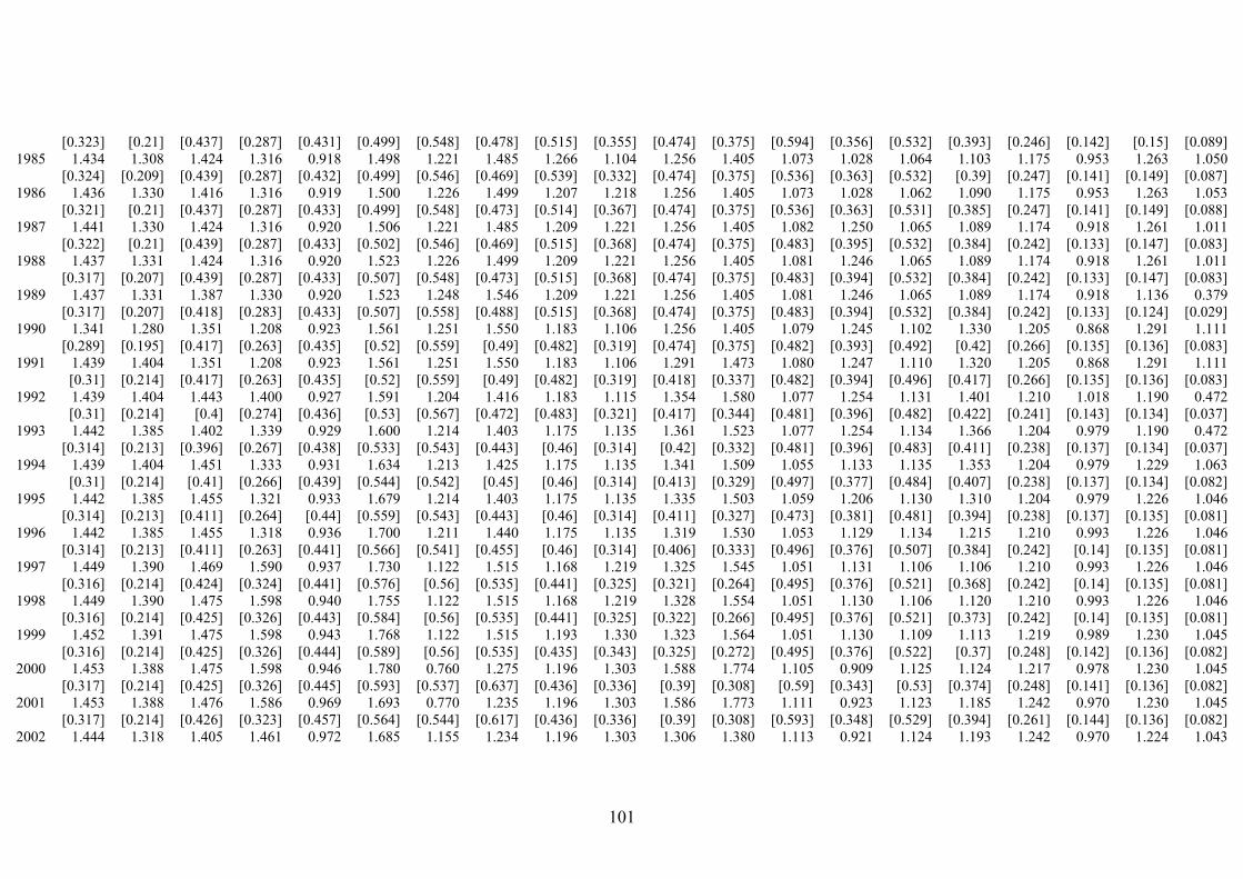
101

[0.323] [0.21] [0.437] [0.287] [0.431] [0.499] [0.548] [0.478] [0.515] [0.355] [0.474] [0.375] [0.594] [0.356] [0.532] [0.393] [0.246] [0.142] [0.15] [0.089] 1985 1.434 1.308 1.424 1.316 0.918 1.498 1.221 1.485 1.266 1.104 1.256 1.405 1.073 1.028 1.064 1.103 1.175 0.953 1.263 1.050 [0.324] [0.209] [0.439] [0.287] [0.432] [0.499] [0.546] [0.469] [0.539] [0.332] [0.474] [0.375] [0.536] [0.363] [0.532] [0.39] [0.247] [0.141] [0.149] [0.087] 1986 1.436 1.330 1.416 1.316 0.919 1.500 1.226 1.499 1.207 1.218 1.256 1.405 1.073 1.028 1.062 1.090 1.175 0.953 1.263 1.053 [0.321] [0.21] [0.437] [0.287] [0.433] [0.499] [0.548] [0.473] [0.514] [0.367] [0.474] [0.375] [0.536] [0.363] [0.531] [0.385] [0.247] [0.141] [0.149] [0.088] 1987 1.441 1.330 1.424 1.316 0.920 1.506 1.221 1.485 1.209 1.221 1.256 1.405 1.082 1.250 1.065 1.089 1.174 0.918 1.261 1.011 [0.322] [0.21] [0.439] [0.287] [0.433] [0.502] [0.546] [0.469] [0.515] [0.368] [0.474] [0.375] [0.483] [0.395] [0.532] [0.384] [0.242] [0.133] [0.147] [0.083] 1988 1.437 1.331 1.424 1.316 0.920 1.523 1.226 1.499 1.209 1.221 1.256 1.405 1.081 1.246 1.065 1.089 1.174 0.918 1.261 1.011 [0.317] [0.207] [0.439] [0.287] [0.433] [0.507] [0.548] [0.473] [0.515] [0.368] [0.474] [0.375] [0.483] [0.394] [0.532] [0.384] [0.242] [0.133] [0.147] [0.083] 1989 1.437 1.331 1.387 1.330 0.920 1.523 1.248 1.546 1.209 1.221 1.256 1.405 1.081 1.246 1.065 1.089 1.174 0.918 1.136 0.379 [0.317] [0.207] [0.418] [0.283] [0.433] [0.507] [0.558] [0.488] [0.515] [0.368] [0.474] [0.375] [0.483] [0.394] [0.532] [0.384] [0.242] [0.133] [0.124] [0.029] 1990 1.341 1.280 1.351 1.208 0.923 1.561 1.251 1.550 1.183 1.106 1.256 1.405 1.079 1.245 1.102 1.330 1.205 0.868 1.291 1.111 [0.289] [0.195] [0.417] [0.263] [0.435] [0.52] [0.559] [0.49] [0.482] [0.319] [0.474] [0.375] [0.482] [0.393] [0.492] [0.42] [0.266] [0.135] [0.136] [0.083] 1991 1.439 1.404 1.351 1.208 0.923 1.561 1.251 1.550 1.183 1.106 1.291 1.473 1.080 1.247 1.110 1.320 1.205 0.868 1.291 1.111 [0.31] [0.214] [0.417] [0.263] [0.435] [0.52] [0.559] [0.49] [0.482] [0.319] [0.418] [0.337] [0.482] [0.394] [0.496] [0.417] [0.266] [0.135] [0.136] [0.083] 1992 1.439 1.404 1.443 1.400 0.927 1.591 1.204 1.416 1.183 1.115 1.354 1.580 1.077 1.254 1.131 1.401 1.210 1.018 1.190 0.472 [0.31] [0.214] [0.4] [0.274] [0.436] [0.53] [0.567] [0.472] [0.483] [0.321] [0.417] [0.344] [0.481] [0.396] [0.482] [0.422] [0.241] [0.143] [0.134] [0.037] 1993 1.442 1.385 1.402 1.339 0.929 1.600 1.214 1.403 1.175 1.135 1.361 1.523 1.077 1.254 1.134 1.366 1.204 0.979 1.190 0.472 [0.314] [0.213] [0.396] [0.267] [0.438] [0.533] [0.543] [0.443] [0.46] [0.314] [0.42] [0.332] [0.481] [0.396] [0.483] [0.411] [0.238] [0.137] [0.134] [0.037] 1994 1.439 1.404 1.451 1.333 0.931 1.634 1.213 1.425 1.175 1.135 1.341 1.509 1.055 1.133 1.135 1.353 1.204 0.979 1.229 1.063 [0.31] [0.214] [0.41] [0.266] [0.439] [0.544] [0.542] [0.45] [0.46] [0.314] [0.413] [0.329] [0.497] [0.377] [0.484] [0.407] [0.238] [0.137] [0.134] [0.082] 1995 1.442 1.385 1.455 1.321 0.933 1.679 1.214 1.403 1.175 1.135 1.335 1.503 1.059 1.206 1.130 1.310 1.204 0.979 1.226 1.046 [0.314] [0.213] [0.411] [0.264] [0.44] [0.559] [0.543] [0.443] [0.46] [0.314] [0.411] [0.327] [0.473] [0.381] [0.481] [0.394] [0.238] [0.137] [0.135] [0.081] 1996 1.442 1.385 1.455 1.318 0.936 1.700 1.211 1.440 1.175 1.135 1.319 1.530 1.053 1.129 1.134 1.215 1.210 0.993 1.226 1.046 [0.314] [0.213] [0.411] [0.263] [0.441] [0.566] [0.541] [0.455] [0.46] [0.314] [0.406] [0.333] [0.496] [0.376] [0.507] [0.384] [0.242] [0.14] [0.135] [0.081] 1997 1.449 1.390 1.469 1.590 0.937 1.730 1.122 1.515 1.168 1.219 1.325 1.545 1.051 1.131 1.106 1.106 1.210 0.993 1.226 1.046 [0.316] [0.214] [0.424] [0.324] [0.441] [0.576] [0.56] [0.535] [0.441] [0.325] [0.321] [0.264] [0.495] [0.376] [0.521] [0.368] [0.242] [0.14] [0.135] [0.081] 1998 1.449 1.390 1.475 1.598 0.940 1.755 1.122 1.515 1.168 1.219 1.328 1.554 1.051 1.130 1.106 1.120 1.210 0.993 1.226 1.046 [0.316] [0.214] [0.425] [0.326] [0.443] [0.584] [0.56] [0.535] [0.441] [0.325] [0.322] [0.266] [0.495] [0.376] [0.521] [0.373] [0.242] [0.14] [0.135] [0.081] 1999 1.452 1.391 1.475 1.598 0.943 1.768 1.122 1.515 1.193 1.330 1.323 1.564 1.051 1.130 1.109 1.113 1.219 0.989 1.230 1.045 [0.316] [0.214] [0.425] [0.326] [0.444] [0.589] [0.56] [0.535] [0.435] [0.343] [0.325] [0.272] [0.495] [0.376] [0.522] [0.37] [0.248] [0.142] [0.136] [0.082] 2000 1.453 1.388 1.475 1.598 0.946 1.780 0.760 1.275 1.196 1.303 1.588 1.774 1.105 0.909 1.125 1.124 1.217 0.978 1.230 1.045 [0.317] [0.214] [0.425] [0.326] [0.445] [0.593] [0.537] [0.637] [0.436] [0.336] [0.39] [0.308] [0.59] [0.343] [0.53] [0.374] [0.248] [0.141] [0.136] [0.082] 2001 1.453 1.388 1.476 1.586 0.969 1.693 0.770 1.235 1.196 1.303 1.586 1.773 1.111 0.923 1.123 1.185 1.242 0.970 1.230 1.045 [0.317] [0.214] [0.426] [0.323] [0.457] [0.564] [0.544] [0.617] [0.436] [0.336] [0.39] [0.308] [0.593] [0.348] [0.529] [0.394] [0.261] [0.144] [0.136] [0.082] 2002 1.444 1.318 1.405 1.461 0.972 1.685 1.155 1.234 1.196 1.303 1.306 1.380 1.113 0.921 1.124 1.193 1.242 0.970 1.224 1.043

102

[0.322] [0.208] [0.397] [0.292] [0.457] [0.561] [0.577] [0.436] [0.436] [0.336] [0.435] [0.325] [0.594] [0.347] [0.529] [0.397] [0.261] [0.144] [0.136] [0.082] 2003 1.433 1.323 1.454 1.509 0.973 1.668 1.152 1.333 1.184 1.213 1.430 1.603 1.060 1.220 1.124 1.200 1.242 0.970 1.196 1.000 [0.312] [0.204] [0.411] [0.301] [0.458] [0.555] [0.615] [0.503] [0.447] [0.324] [0.396] [0.314] [0.474] [0.385] [0.529] [0.399] [0.261] [0.144] [0.13] [0.077] 2004 1.456 1.388 1.454 1.509 0.974 1.660 1.152 1.333 1.175 1.203 1.430 1.603 1.059 1.221 1.121 1.213 1.242 0.970 1.233 1.081 [0.329] [0.222] [0.411] [0.301] [0.459] [0.553] [0.615] [0.503] [0.444] [0.321] [0.396] [0.314] [0.473] [0.386] [0.528] [0.404] [0.261] [0.144] [0.132] [0.081] 2005 1.456 1.388 1.448 1.510 0.974 1.663 1.131 1.290 1.175 1.203 1.274 1.338 1.057 1.225 1.119 1.221 1.244 0.965 1.226 1.076 [0.329] [0.222] [0.409] [0.301] [0.459] [0.554] [0.604] [0.487] [0.444] [0.321] [0.437] [0.324] [0.472] [0.387] [0.527] [0.406] [0.265] [0.145] [0.134] [0.083] 2006 1.445 1.398 1.445 1.509 0.974 1.664 1.125 1.276 1.168 1.198 1.254 1.321 1.057 1.224 1.118 1.236 1.244 0.965 1.224 1.098 [0.327] [0.223] [0.408] [0.301] [0.459] [0.554] [0.601] [0.482] [0.441] [0.32] [0.43] [0.32] [0.472] [0.387] [0.527] [0.412] [0.265] [0.145] [0.13] [0.082] 2007 1.445 1.398 1.442 1.583 0.974 1.663 1.121 1.269 1.151 1.220 1.258 1.391 1.099 0.910 1.114 1.249 1.241 0.976 1.229 1.078 [0.327] [0.223] [0.416] [0.323] [0.459] [0.554] [0.598] [0.479] [0.435] [0.326] [0.419] [0.327] [0.587] [0.343] [0.525] [0.416] [0.264] [0.147] [0.132] [0.082]

103

Table A.5.2.1. The dynamics of the regression estimate of the Pareto exponent

0.50

0.75

1.00

1.25

1.50

1.75

1970 1975 1980 1985 1990 1995 2000 20050.00

0.25

0.50

0.75

1.00

1.25

1.50

1.75

2.00

1970 1975 1980 1985 1990 1995 2000 2005

a. Russian Federation b. Ukraine

0.60

0.80

1.00

1.20

1.40

1.60

1.80

2.00

2.20

1970 1975 1980 1985 1990 1995 2000 20050.30

0.65

1.00

1.35

1.70

2.05

1970 1975 1980 1985 1990 1995 2000 2005

c. Poland d. Romania

0.00

0.40

0.80

1.20

1.60

2.00

2.40

1970 1975 1980 1985 1990 1995 2000 2005-0.20

0.10

0.40

0.70

1.00

1.30

1.60

1.90

2.20

2.50

2.80

1970 1975 1980 1985 1990 1995 2000 2005

e. Former Yugoslavia f. Belarus

-0.20

0.20

0.60

1.00

1.40

1.80

2.20

1970 1975 1980 1985 1990 1995 2000 2005-0.20

0.00

0.20

0.40

0.60

0.80

1.00

1.20

1.40

1.60

1.80

2.00

1970 1975 1980 1985 1990 1995 2000 2005

g. Baltic States h. Hungary

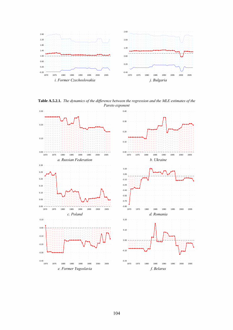
104

-0.20

0.20

0.60

1.00

1.40

1.80

2.20

2.60

1970 1975 1980 1985 1990 1995 2000 2005-0.40

0.20

0.80

1.40

2.00

2.60

1970 1975 1980 1985 1990 1995 2000 2005

i. Former Czechoslovakia j. Bulgaria

Table A.5.2.1. The dynamics of the difference between the regression and the MLE estimates of the Pareto exponent

0.00

0.10

0.20

0.30

1970 1975 1980 1985 1990 1995 2000 20050.00

0.10

0.20

0.30

0.40

1970 1975 1980 1985 1990 1995 2000 2005

a. Russian Federation b. Ukraine

0.00

0.05

0.10

0.15

0.20

0.25

0.30

1970 1975 1980 1985 1990 1995 2000 2005-0.85

-0.70

-0.55

-0.40

-0.25

-0.10

0.05

0.20

1970 1975 1980 1985 1990 1995 2000 2005

c. Poland d. Romania

-0.40

-0.30

-0.20

-0.10

0.00

0.10

1970 1975 1980 1985 1990 1995 2000 2005-0.20

-0.10

0.00

0.10

0.20

1970 1975 1980 1985 1990 1995 2000 2005

e. Former Yugoslavia f. Belarus

105

-0.30

-0.15

0.00

0.15

1970 1975 1980 1985 1990 1995 2000 2005-0.90

-0.75

-0.60

-0.45

-0.30

-0.15

0.00

1970 1975 1980 1985 1990 1995 2000 2005

g. Baltic States h. Hungary

-0.30

-0.15

0.00

0.15

0.30

1970 1975 1980 1985 1990 1995 2000 2005-0.60

-0.45

-0.30

-0.15

0.00

1970 1975 1980 1985 1990 1995 2000 2005

i. Former Czechoslovakia j. Bulgaria

106

Table A5.3.1. Parameters of regression of logarithms of city ranks i for largest cities in Russia (with the population above 100 thousand people) against the logarithms of

city size Ni: ln(i-1/2) = a - ζ·ln Ni

Dependent variable Logarithm of city ranks ln(i-1/2) Years 1897 1926 1939 1959 1970

Independent variable Regression coefficient

Constant

lnNi

R2 F(R2)

5.589910 (0.748386) -0.824135 (0.135973)

0.860 36.74

7.920504 (0.487601) -1.113586 (0.090925)

0.893 150.00

9.900424 (0.258400) -1.275446 (0.046920)

0.938 738.94

10.59869 (0.185453) -1.303802 (0.032391)

0.961 1620.21

10.96055 (0.209420) -1.297354 (0.035298)

0.949 1350.90

Sample size n=8 n=20 n=51 n=66 n=75 Years 1979 1989 2002 2003 2004

Independent variable Regression coefficient

Constant

lnNi

R2 F(R2)

11.01538 (0.116334) -1.266171 (0.020597)

0.965 3778.86

11.00539 (0.124625) -1.237672 (0.021873)

0.956 3201.90

10.92802 (0.113270) -1.227856 (0.020085)

0.960 3737.37

10.92045 (0.113024) -1.226676 (0.020043)

0.960 3745.54

10.93742 (0.112480) -1.229840 (0.019950)

0.960 3800.33

Sample size n=138 n=151 n=159 n=159 n=159 Years 2005 2006 2007 2008 2009

Independent variable Regression coefficient

Constant

lnNi

R2 F(R2)

10.96038 (0.108596) -1.233169 (0.019318)

0.962 4075.05

10.97003 (0.109227) -1.234586 (0.019426)

0.962 4039.18

10.96880 (0.108756) -1.234937 (0.019351)

0.962 4072.86

10.96678 (0.108854) -1.234633 (0.019369)

0.962 4063.22

10.95741 (0.107797) -1.232836 (0.019195)

0.962 4125.06

Sample size n=163 n=163 n=163 n=163 n=164

Table A5.3.2. Parameters of the regression of the logarithm of the population of Russian cities (except for Moscow and Saint-Petersburg) against their rank for the

years 1897-2009

Dependent Variable Logarithm of the population Ni

Independent variable

Regression coefficient 1897 1926 1939 1959 1970 1979

Const i

R2... F(R2)

5.078591 -0.040165

0.848 518.01

5.819091 -0.049725

0.888 562.24

6.462330 -0.041254

0.857 449.02

6.801082 -0.036110

0.854 439.91

6.959886 -0.030297

0.900 677.90

6.715370 -0.016405

0.943 2610.93

Included 95 73 77 77 77 159

107

observations

Dependent Variable Logarithm of the population Ni

Independent variable

Regression coefficient 1989 2002 2003 2004 2005 2006

Const i

R2... F(R2)

6.823465 -0.015847

0.948 2894.26

6.761217 -0.015022

0.956 3478.67

6.757072 -0.014964

0.956 3488.50

6.755904 -0.014973

0.956 3423.99

6.736914 -0.014572

0.950 3062.22

6.736782 -0.014553

0.951 3082.90

Included observations 162 161 162 161 162 162

Dependent Variable Logarithm of the population Ni

Independent variable

Regression coefficient 2007 2008 2009

Const i

R2... F(R2)

6.733465 -0.014545

0.950 3059.02

6.733453 -0.014547

0.951 3073.39

6.734632 -0.014545

0.950 3046.31

Included observations 162 162 162

Note: The coefficients are significant if the significance level is above 0.00005. R2 is significant if the significance level is not larger than 0.0000005.

Table A5.3.3. Parameters of regression of c and k agaist ranks Years and political variables P1, P2, P3 for the cities in Russia

Dependent variable

c c c c k Model 1 Model 2 Model 3 Model 4 Independent

variable Regression coefficient Regression coefficient

Const t

P1

P2

P3

R2 F(R2) DW

-4.889177 (11.36847) 0.005254

(0.005992) 0.875585

(0.280179) 0.464865

(0.281449) -0.245474 (0.208275)

0.933 35.09 2.613

5.078591 (0.146145)

---

1.062120 (0.178990) 0.630060

(0.111620) ---

0.923 72.02 2.743

-31.47273 (4.668597) 0.019399

(0.002392) ---

---

-0.687989 (0.163097)

0.869 39.64 1.179

---

0.002678 (7.55E-05) 0.966226

(0.177637) 0.572450

(0.124103) -0.164946 (0.087757)

0.932 ---

2.859

-1.349853 (0.171911) 0.000690

(9.06E-05) -0.029829 (0.004237) -0.008002 (0.004256) -0.011622 (0.003149)

0.977 106.57 2.329

Sample size n=15

108

Note: Standard errors of the regression coefficients are given in brackets. Table A5.3.4. Parameters of the regression of the logarithm of the population of Belarusian cities against their rank (lnSize=C+к Rank) for the years 1970-2009

Years N Variabl

e Coefficien

t Std.Erro

r

t-statisti

c p R2

F-statisti

c

1970 198

Rank -0.018014 0.0006 -29.560 0.0000 0.81

7 873.80 C 3.656932 0.0699 52.297 0.000

0

1979 200

Rank -0.019605 0.0006 -33.610 0.0000 0.85

1 1129.6

2 C 4.017004 0.0676 59.418 0.0000

1989 202

Rank -0.020990 0.0006 -37.683 0.0000 0.87

7 1420.0

2 C 4.333892 0.0652 66.468 0.0000

1990 202

Rank -0.021041 0.0006 -37.946 0.0000 0.87

8 1439.9

1 C 4.366013 0.0649 67.264 0.0000

1991 202

Rank -0.021133 0.0006 -38.365 0.0000 0.88

0 1471.9

0 C 4.382248 0.0645 67.963 0.0000

1992 202

Rank -0.021238 0.0006 -38.535 0.0000 0.88

1 1484.9

3 C 4.398832 0.0645 68.183 0.0000

1993 202

Rank -0.021356 0.0005 -39.016 0.0000 0.88

4 1522.2

2 C 4.416907 0.0641 68.936 0.0000

1994 202

Rank -0.021437 0.0005 -39.377 0.0000 0.88

6 1550.5

5 C 4.432715 0.0637 69.557 0.0000

1995 202

Rank -0.021431 0.0005 -39.341 0.0000 0.88

6 1547.7

4 C 4.437681 0.0638 69.593 0.0000

1997 203

Rank -0.021565 0.0005 -40.505 0.0000 0.89

1 1640.6

8 C 4.457189 0.0626 71.168 0.0000

1998 20 Rank -0.021255 0.0005 -39.865 0.000 0.88 1589.2

109

5 0 7 2

C 4.434770 0.0633 70.021 0.0000

1999 205

Rank -0.021485 0.0005 -40.402 0.0000 0.88

9 1632.3

2 C 4.423677 0.0632 70.029 0.0000

2000 205

Rank -0.021539 0.0005 -40.513 0.0000 0.89

0 1641.3

4 C 4.428232 0.0632 70.118 0.0000

2001 207

Rank -0.021282 0.0005 -40.434 0.0000 0.88

9 1634.8

7 C 4.414205 0.0631 69.921 0.0000

2002 207

Rank -0.021354 0.0005 -40.476 0.0000 0.88

9 1638.3

0 C 4.416414 0.0633 69.792 0.0000

2003 206

Rank -0.021361 0.0005 -40.089 0.0000 0.88

7 1607.1

6 C 4.412470 0.0636 69.376 0.0000

2004 206

Rank -0.021384 0.0005 -40.065 0.0000 0.88

7 1605.2

2 C 4.409145 0.0637 69.207 0.0000

2005 206

Rank -0.021489 0.0005 -40.056 0.0000 0.88

7 1604.4

8 C 4.410506 0.0640 68.874 0.0000

2006 206

Rank -0.021573 0.0005 -40.143 0.0000 0.88

8 1611.4

2 C 4.411310 0.0641 68.767 0.0000

2007 207

Rank -0.021660 0.0005 -40.484 0.0000 0.88

9 1638.9

9 C 4.414477 0.0642 68.791 0.0000

2008 206

Rank -0.021725 0.0005 -40.246 0.0000 0.88

8 1619.7

5 C 4.416968 0.0644 68.549 0.0000

2009 206

Rank -0.021776 0.0005 -40.365 0.0000 0.88

9 1629.3

3 C 4.421704 0.0644 68.665 0.0000

110

Table A5.3.5. Parameters of the regression of the logarithm of the population of Belarusian cities against their rank (lnSize=C+к Rank) for the years 1970-2009

without MINSK

Years N Variabl

e Coefficien

t Std.Erro

r

t-statisti

c p R2

F-statisti

c

1970 197

Rank -0.017521 0.0005 -32.184 0.0000 0.84

2 1035.8

3 C 3.591554 0.0626 57.349 0.0000

1979 199

Rank -0.019126 0.0005 -36.860 0.0000 0.87

3 1358.6

3 C 3.952871 0.0603 65.563 0.0000

1989 201

Rank -0.020532 0.0005 -41.469 0.0000 0.89

6 1719.6

6 C 4.271895 0.0581 73.525 0.0000

1990 201

Rank -0.020587 0.0005 -41.711 0.0000 0.89

7 1739.8

0 C 4.304593 0.0579 74.320 0.0000

1991 201

Rank -0.020689 0.0005 -42.012 0.0000 0.89

9 1765.0

3 C 4.322171 0.0578 74.792 0.0000

1992 201

Rank -0.020786 0.0005 -42.394 0.0000 0.90

0 1797.2

4 C 4.337667 0.0575 75.389 0.0000

1993 201

Rank -0.020905 0.0005 -42.982 0.0000 0.90

3 1847.4

5 C 4.355911 0.0571 76.320 0.0000

1994 201

Rank -0.020989 0.0005 -43.402 0.0000 0.90

4 1883.7

4 C 4.371978 0.0567 77.042 0.0000

1995 201

Rank -0.020982 0.0005 -43.351 0.0000 0.90

4 1879.2

9 C 4.376965 0.0568 77.062 0.0000

1997 202

Rank -0.021123 0.0005 -44.775 0.0000 0.90

9 2004.8

2 C 4.397009 0.0556 79.039 0.0000

1998 204

Rank -0.020815 0.0005 -43.967 0.0000 0.90

5 1933.1

2 C 4.374362 0.0564 77.594 0.000

111

0

1999 204

Rank -0.021047 0.0005 -44.558 0.0000 0.90

8 1985.4

4 C 4.363493 0.0562 77.578 0.0000

2000 204

Rank -0.021101 0.0005 -44.687 0.0000 0.90

8 1996.9

1 C 4.368049 0.0562 77.683 0.0000

2001 206

Rank -0.020849 0.0005 -44.567 0.0000 0.90

7 1986.1

9 C 4.354215 0.0562 77.411 0.0000

2002 206

Rank -0.020921 0.0005 -44.609 0.0000 0.90

7 1989.9

5 C 4.356310 0.0564 77.256 0.0000

2003 205

Rank -0.020921 0.0005 -44.217 0.0000 0.90

6 1955.1

3 C 4.351832 0.0566 76.865 0.0000

2004 205

Rank -0.020943 0.0005 -44.217 0.0000 0.90

6 1955.1

1 C 4.348269 0.0567 76.723 0.0000

2005 205

Rank -0.021046 0.0005 -44.194 0.0000 0.90

6 1953.1

0 C 4.349380 0.0570 76.327 0.0000

2006 205

Rank -0.021129 0.0005 -44.300 0.0000 0.90

6 1962.5

3 C 4.350032 0.0571 76.222 0.0000

2007 206

Rank -0.021219 0.0005 -44.648 0.0000 0.90

7 1993.4

6 C 4.353375 0.0571 76.184 0.0000

2008 205

Rank -0.021279 0.0005 -44.416 0.0000 0.90

7 1972.7

6 C 4.355422 0.0573 75.975 0.0000

2009 205

Rank -0.021329 0.0005 -44.570 0.0000 0.90

7 1986.4

5 C 4.360096 0.0573 76.140 0.0000

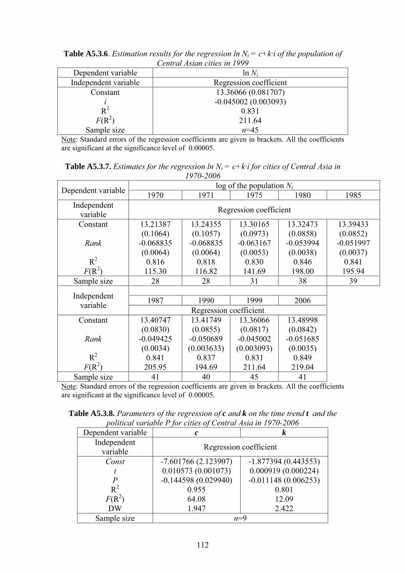
112

Table A5.3.6. Estimation results for the regression ln Ni = c+k·i of the population of Central Asian cities in 1999

Dependent variable ln Ni Independent variable Regression coefficient

Constant i

R2 F(R2)

Sample size

13.36066 (0.081707) -0.045002 (0.003093)

0.831 211.64 n=45

Note: Standard errors of the regression coefficients are given in brackets. All the coefficients are significant at the significance level of 0.00005. Table A5.3.7. Estimates for the regression ln Ni = c+k·i for cities of Central Asia in

1970-2006

Dependent variable log of the population Ni 1970 1971 1975 1980 1985

Independent variable Regression coefficient

Constant

Rank

R2 F(R2)

13.21387 (0.1064)

-0.068835 (0.0064)

0.816 115.30

13.24355 (0.1057)

-0.068835 (0.0064)

0.818 116.82

13.30165 (0.0973)

-0.063167 (0.0053)

0.830 141.69

13.32473 (0.0858)

-0.053994 (0.0038)

0.846 198.00

13.39433 (0.0852)

-0.051997 (0.0037)

0.841 195.94

Sample size 28 28 31 38 39

Independent variable

1987 1990 1999 2006

Regression coefficient Constant

Rank

R2

F(R2)

13.40747 (0.0830)

-0.049425 (0.0034)

0.841 205.95

13.41749 (0.0855)

-0.050689 (0.003633)

0.837 194.69

13.36066 (0.0817)

-0.045002 (0.003093)

0.831 211.64

13.48998 (0.0842)

-0.051685 (0.0035)

0.849 219.04

Sample size 41 40 45 41 Note: Standard errors of the regression coefficients are given in brackets. All the coefficients are significant at the significance level of 0.00005.

Table A5.3.8. Parameters of the regression of c and k on the time trend t and the political variable P for cities of Central Asia in 1970-2006

Dependent variable c k Independent

variable Regression coefficient

Const t P R2

F(R2) DW

-7.601766 (2.123907) 0.010573 (0.001073) -0.144598 (0.029940)

0.955 64.08 1.947

-1.877394 (0.443553) 0.000919 (0.000224) -0.011148 (0.006253)

0.801 12.09 2.422

Sample size n=9

113

Note: Standard errors of the regression coefficients are given in brackets.

Table A5.3.9. Estimation results for the regression ln Ni = c+k·i of the population of Caucasus cities in 2007 Dependent variable ln Ni

Independent variable Regression coefficient Constant

i R2

F(R2) Sample size

14.50335 (0.240176) -0.336194 (0.038708)

0.904 75.44 n=10

Note: Standard errors of the regression coefficients are given in brackets. All the coefficients are significant at the significance level of 0.00005. Table A5.3.10. Parameters of regression of logarithms of the population Ni for cities

of Caucasus agaist its ranks: ln Ni =c+k·i

Dependent variable

log of the population Ni 1970 1971 1975 1980

Independent variable Regression coefficient

Constant Rank

R2 F(R2)

13.86252 (0.2725) -0.276535 (0.0439)

0.832 39.63

13.88072 (0.2747)

-0.274877 (0.0443)

0.828 38.56

13.98215 (0.2970) -0.257304 (0.0438)

0.793 34.52

14.12501 (0.2799) -0.261800 (0.0413)

0.817 40.24

Sample size 10 10 11 11

Independent variable

1985 1987 1990 2007 Regression coefficient

Constant Rank

2 F(R2)

14.21326 (0.2773) -0.262220 (0.0409)

0.820 41.14

14.24711 (0.2751) -0.262647 (0.0406)

0.823 41.93

14.29858 (0.2583) -0.299119 (0.0416)

0.866 51.62

14.50335 (0.2402) -0.336194 (0.0387)

0.904 75.44

Sample size 11 11 10 10

Table A5.3.11. Parameters of the regression of c and k on the time trend t and the

political variable P for cities of Caucasus in 1970-2007 Dependent variable c k

Independent variable Regression coefficient Const Year

P R2

F(R2) DW

-30.22902 (1.815403) 0.022385 (0.000917) -0.194493 (0.031475)

0.995 535.60 1.4994

-0.270643 (0.005465) ---

-0.065551 (0.015458) 0.750 17.98 1.9714

Sample size n=8 Note: Standard errors of the regression coefficients are given in brackets.

114

Table A5.3.12. Parameters of the regression of logarithms ln4 of the population Ni for the populated areas of Russia (except for Moscow and Saint-Petersburg) in the years

1897-2009 against their ranks i: ln4 Ni = c+k·i Dependent Variable ln4 Ni

Independent variable Regression coefficient

1897 1926 1939 1959 1970 1979Const

i R2... F(R2)

-0.162999 -0.043392

0.760 206.36

-0.432231-0.019682

0.812 250.31

-0.310213-0.013837

0.631 123.29

-0.289375-0.010744

0.323 35.36

-0.351581 -0.006421

0.655 142.61

-0.396210-0.003505

0.975 6090.79

Sample size 67 60 74 76 77 158Dependent Variable ln4 Ni

Independent variable

Regression coefficient1989 2002 2003 2004 2005 2006

Const i

R2... F(R2)

-0.365500 -0.003580

0.556 200.50

-0.400339-0.003003

0.986 11079.18

-0.400607-0.003001

0.986 11666.09

-0.401202-0.002994

0.985 10506.97

-0.407275 -0.002870

0.994 26019.70

-0.407282-0.002866

0.994 25547.44

Sample size 162 161 162 161 162 162Dependent Variable ln4 Ni

Independent variable

Regression coefficient2007 2008 2009

Const i

R2... F(R2)

-0.407732 -0.002867

0.994 25553.24

-0.407672-0.002868

0.994 26221.30

-0.407659-0.002865

0.994 26060.48

Sample size 162 162 162

Table A5.3.12. Parameters of the regression coefficient c4 of the equation ln4Ni =c4+k4i for time t (except for Moscow and Saint-Petersburg)

Dependent variable C4Independent

variable Regression coefficient

Const t

R2 F(R2) DW

-0.258998 (0.032879) -0.001264 (0.000285)

0.767 19.72 1.479

Sample size n=8 (2002-2009 years) Note. Standard errors of the regression coefficients are given in brackets. The regression coefficients are significant at the significance level not larger than 0.0045; R2 is significant at the significance level not larger than 0.0044.

115

Table A5.3.13. Parameters of the regression coefficients k4 of the equation ln4Ni =c4+k4i for time t (except for Moscow and Saint-Petersburg)

Dependent variable k4Independent

variable Regression coefficient

Const lnt R2

F(R2) DW

-0.071110 (0.001650) 0.014469 (0.000375)

0.991347 1489.387 1.114548

Sample size n=15 Note. Standard errors of the regression coefficients are given in brackets. The regression coefficients are significant at the significance level not larger than 0.0000005; R2 is significant at the significance level not larger than 0.0000005

Table A5.3.14. Regression lnr Ni = c+k·i of the logarithm iterations lnr Ni on the ranks i of city sizes Ni of the Central Asian cities in 1999

Dependent variable

Hierarchy of logarithms of the population Ni Ln(Ni) Ln2(Ni) Ln3(Ni) Ln4(Ni)

Independent variable

Regression coefficient

Regression coefficient

Regression coefficient

Regression coefficient

Constant

Rank

R2 F(R2)

13.36066 (0.081707) -0.045002 (0.003093)

0.831 211.64

2.592944 (0.005919) -0.003590 (0.000224)

0.856 256.62

0.952914 (0.002253) -0.001421 (8.53E-05)

0.866 277.41

-0.048076 (0.002331) -0.001534 (8.83E-05)

0.875 301.98

Sample size n=45 Note: Standard errors of the regression coefficients are given in brackets. All the coefficients are significant at the significance level of 0.00005.

Table A5.3.15. Regression lnr Ni = c+k·i of the logarithm iterations lnr Ni on the ranks i of city sizes Ni of the Caucasus in 2007

Dependent variable Hierarchy of logarithms of the population Ni Ln(Ni) Ln2(Ni) Ln3(Ni) Ln4(Ni)

Independent variable Regression coefficient Constant

Rank

R2

F(R2)

14.50335 (0.240176) -0.336194 (0.038708)

0.904 75.44

2.678939 (0.017464) -0.026196 (0.002815)

0.915 86.62

0.986183 (0.006662) -0.010276 (0.001074)

0.920 91.62

-0.013023 (0.006911) -0.010991 (0.001114)

0.924 97.39

Sample size n=10 Note: Standard errors of the regression coefficients are given in brackets. All the coefficients are significant at the significance level of 0.00005.

116

Table A.5.4.1. Description of the dataset for the “within” distribution analysis

Country Investigated period by decades

Numbers of cities

Poland 1961-2004 890 Belarus 1970-2009 207 Hungary 1970-2001 237 Russia 1897-2002 479

Table A.5.4.2. Values of LR statistics to test Markovity of Polish cities distribution

Years 1961 1974 1985 1994 LR(O(0)) 1943.578 1966.536 2562.915 2880.135LR(O(1)) -396.545 -402.227 -478.677

Table A.5.4.3. The probability of acceptance of Markovity of appropriate order in Poland Years DF 1961 1974 1985 1994

0 order Markovity

36 0 0 0 0

≥ 1 order Markovity

28 1 1 1 1

DF - Degrees of freedom Table A.5.4.4. Values of LR statistics to test Markovity of Belarusian cities distribution

Years 1970 1979 1989 1999

LR(O(0)) 478.2052689 563.5174 566.3945 548.5899 LR(O(1)) -100.6281285 -103.289 -115.623

Table A.5.4.5. The probability of acceptance of Markovity of appropriate order in Belarus Years DF 1970 1979 1989 1999 0 order Marcovity

36 1.19068E-78 5.72E-96 1.48E-96 6.33E-93

≥ 1 order Marcovity

14 1 1 1 1

DF - Degrees of freedom

Table A.5.4.6. Values of LR statistics to test Markovity of Hungarian cities distribution

Years 1880 1890 1900 1910 1920 1930 1940 1950 1960 1970 1980 1990 2001

LR(O(0)) 662 693 558 662 698 672 642 657 501 555 570 689 702

LR(O(1)) 6.55 12.8 8.3 5.4 5.7 10.3 16.4 23.5 13.8 5.9 -0.64721 1.73

117

Table A.5.4.7. The probability of acceptance of Markovity of appropriate order in Hungary (1880-1940)

Years DF 1880 1890 1900 1910 1920 1930 1940

0 order Marcovity 36 2.9E-

116 1.5E-122 6.3E-95 2.9E-116 1.2E-123 2.5E-118 3.6E-112

≥ 1 order Marcovity 22 0.9993 0.9395 0.9963 0.9998 0.9998 0.983 0.7955

DF - Degrees of freedom Table A.5.4.8. The probability of acceptance of Markovity of appropriate order in Hungary (1950-2001)

Years DF 1950 1960 1970 1980 1990 2001

0 order Marcovity is 36 4E-

115 2.74E-83 2.93E-94 2.22E-97 1E-121 2.2E-124

≥ 1 order Marcovity 22 0.374 0.90 0.9997 1 1

DF - Degrees of freedom

Table A.5.4.9. Values of LR statistics to test Markovity of Russian cities distribution

Years 1897 1926 1939 1959 1970 1979 LR(O(0)) 605.109 599.7309 938.1978 1211.197 1340.7 1358.753 LR(O(1)) 45.33589 64.50166 17.65158 36.06105 43.01439 41.3714

Table A.5.4.10. The probability of acceptance of Markovity of appropriate order in Russia

Years DF 1897 1926 1939 1959 1970 1979

0 order Marcovity 36 1.8E-104 2.2E-103 1.4E-173 5.6E-231 2.4E-258 3.6E-262

≥ 1 order Marcovity 67 0.980458 0.563856 1 0.9992 0.99007 0.99418

118

Table A.5.4.11. Probability transition matrix for Poland, 1961-2004

1 2 3 4 5 6 7 Number of observations <10% <20% <30% <50% <100% <200% >200%

1 0.786 0.155 0.024 0.0065 0.026 0.002 0 459 2 0.072 0.838 0.082 0.004 0.0028 0.0014 0 722 3 0.004 0.123 0.73 0.14 0.002 0 0 480 4 0.002 0 0.0687 0.77 0.147 0.0076 0 524 5 0.003 0.003 0 0.027 0.888 0.072 0.005 582 6 0.004 0.0035 0 0.0035 0.042 0.866 0.081 284 7 0 0 0 0 0 0.02 0.979 290

Table A.5.4.12. Probability transition matrix for Belarus, 1970-2009

1 2 3 4 5 6 7 Number of observations <10% <20% <30% <50% <100% <200% >200%

1 0.944 0.043 0.012 0 0 0 0 162 2 0.265 0.649 0.086 0 0 0 0 151 3 0 0.106 0.807 0.087 0 0 0 161 4 0 0 0.128 0.832 0.040 0 0 149 5 0 0 0 0.149 0.824 0.027 0 74 6 0 0 0 0 0.098 0.854 0.049 41 7 0 0 0 0 0 0.027 0.973 75 Table A.5.4.13. Probability transition matrix for Hungary, 1970-2001

1 2 3 4 5 6 7 Number of observations <10% <20% <30% <50% <100% <200% >200%

1 0.87 0.12 0 0.01 0 0 0 151 2 0.03 0.88 0.077 0.003 0.005 0.003 0 376 3 0 0.086 0.82 0.09 0.003 0.001 0 427 4 0 0 0.1 0.85 0.05 0 0 729 5 0 0 0 0.1 0.88 0.02 0 786 6 0 0 0 0 0.09 0.88 0.03 388 7 0 0 0 0 0 0.08 0.92 224

Table A.5.14. Probability transition matrix for Russia, 1897-2002

1 2 3 4 5 6 7 Number of observations <10% <20% <30% <50% <100% <200% >200%

1 0.92 0.05 0.017 0.011 0.002 0 0 524 2 0.179 0.736 0.057 0.021 0.006 0 0.001 700 3 0.022 0.330 0.525 0.100 0.022 0 0 448 4 0.002 0.057 0.232 0.609 0.092 0.007 0.002 557 5 0 0.016 0.028 0.220 0.654 0.069 0.014 509 6 0 0 0 0.004 0.152 0.726 0.119 270 7 0 0 0 0 0.003 0.061 0.936 345

119

Table A.5.4.2.15. Mean first passage time matrix for Poland, years

Class 1 2 3 4 5 6 7 <10% <20% <30% <50% <100% <200% >200%

1 588 920 115 850 417 536 827 2 2053 260 739 689 430 550 843 3 3438 1890 476 380 340 470 760 4 4659 3480 2600 340 188 340 610 5 5173 413 3690 1955 100 226 487 6 5556 4530 4160 2590 1020 60 290 7 6060 5020 4630 3076 1520 470 17 Table A.5.4.2.16. Mean first passage time matrix for Belarus, years

Class 1 2 3 4 5 6 7 <10% <20% <30% <50% <100% <200% >200%

1 18 220 490 1085 3200 15840 40077 2 99 80 400 994 3110 15750 39980 3 290 190 63 597 2716 15340 39585 4 410 300 117 91 212 14720 38980 5 530 420 238 120 330 12510 36830 6 820 700 529 410 290 1250 24620 7 1190 1070 907 780 660 386 670 Table A.5.4.2.17. Mean first passage time matrix for Hungary, years

Class 1 2 3 4 5 6 7 <10% <20% <30% <50% <100% <200% >200%

1 188.7 124.8 254 390 725 2618.8 8168.8 2 1300 45.5 178.8 348 672 2551 8107 3 1620 320 43.5 228 590 2508 8068 4 1795 495 174 40 440 2435 8000 5 1920 622 302 130 58.8 2118 7710 6 2077.6 778 457.8 289 157 200 5780 7 2195 895 576 409 276 124 500 Table A.5.4.2.18. Mean first passage time matrix for Russia, years

Class 1 2 3 4 5 6 7 <10% <20% <30% <50% <100% <200% >200%

1 20 160 318 497 1060 2900 4477 2 95 47 270 460 1020 2850 4420 3 144 60 125 370 936 2780 4350 4 200 120 130 140 739 2580 4160 5 290 210 227 1690 230 2030 3646 6 469 380 400 346 190 357 2110 7 617 530 550 498 340 247 150

120

Table A.5.4.2.19. Initial and ergodic distributions for Polish cities

1 2 3 4 5 6 7 <10% <20% <30% <50% <100% <200% >200%

Initial distribution 0.137 0.216 0.14 0.157 0.174 0.085 0.087

Ergodic distribution 0.017 0.038 0.02 0.029 0.1 0.156 0.64

Table A.5.4.20. Initial and ergodic distributions for Belarusian cities

1 2 3 4 5 6 7 <10% <20% <30% <50% <100% <200% >200%

Initial distribution 0.199 0.186 0.198 0.183 0.091 0.05 0.092

Ergodic distribution 0.56 0.12 0.16 0.11 0.03 0.008 0.015 Table A.5.4.21. Initial and ergodic distributions for Hungarian cities

1 2 3 4 5 6 7 <10% <20% <30% <50% <100% <200% >200%

Initial distribution 0.049 0.122 0.139 0.237 0.255 0.126 0.073

Ergodic distribution 0.053 0.22 0.23 0.25 0.17 0.05 0.02

Table A.5.4.22. Initial and ergodic distributions for Russian cities

1 2 3 4 5 6 7 <10% <20% <30% <50% <100% <200% >200%

Initial distribution 0.156 0.209 0.134 0.166 0.152 0.081 0.103

Ergodic distribution 0.497 0.212 0.08 0.07 0.043 0.028 0.067

Table A.5.4.23 Initial vs ergodic distribution 1900—2001: Spain

1 2 3 4 5 6 <20% <50% <80% <135% <185% >185%

Initial distribution

0.356 0.243 0.143 0.118 0.044 0.098

Ergodic distribution

0.254 0.355 0.181 0.098 0.035 0.078

121

Table A.5.4.24. The values of kurtosis across countries

Poland Belarus Hungary Russia

Initial distr. -0.40628 -1.98351 -0.98227 -0.00516 Ergodic distr. 5.84045 5.03177 -2.41139 4.18436

Difference 4.99726 6.80950 -1.64034 5.75212 Figure A.5.4.1 Initial vs ergodic distributions (Blue – Initial, Red – Ergodic).

Polish Initial vs Ergodic distribution

0

0.1

0.2

0.3

0.4

0.5

0.6

0.7

1 2 3 4 5 6 7

Belarusian Initial vs Ergodic distribution

0

0.1

0.2

0.3

0.4

0.5

0.6

0.7

1 2 3 4 5 6 7

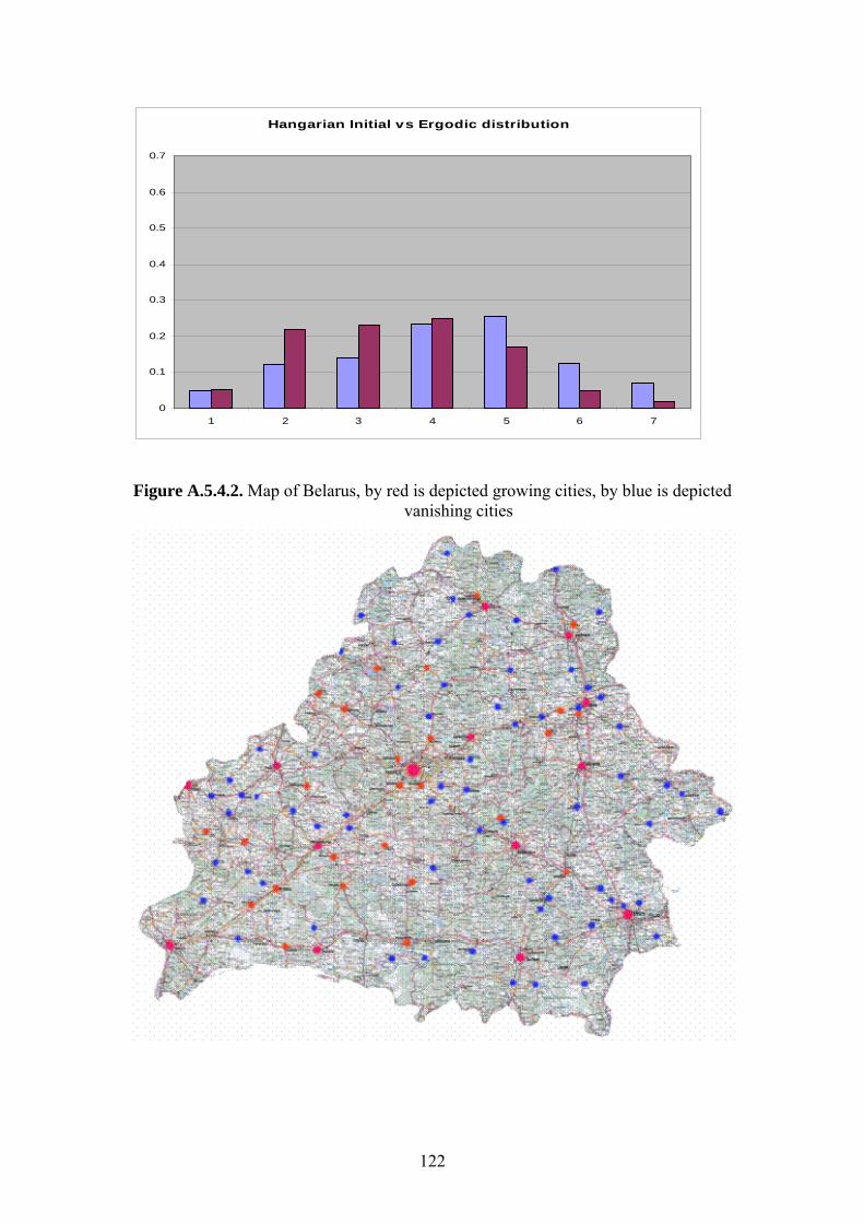
122

Hangarian Initial vs Ergodic distribution

0

0.1

0.2

0.3

0.4

0.5

0.6

0.7

1 2 3 4 5 6 7

Figure A.5.4.2. Map of Belarus, by red is depicted growing cities, by blue is depicted vanishing cities

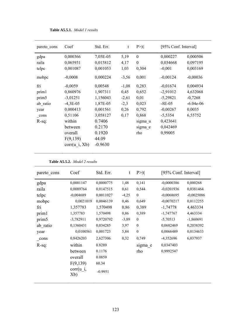
123

Table A5.5.1. Model 1 results

pareto_cons Coef Std. Err. t P>|t| [95% Conf. Interval]

gdpa 0,000366 7,05E-05 5,19 0 0,000227 0,000506 raila 0,065931 0,015812 4,17 0 0,034668 0,097195 telpc 0,001087 0,001053 1,03 0,304 -0,001 0,003169

mobpc -0,0008 0,000224 -3,56 0,001 -0,00124 -0,00036

fri -0,0059 0,00548 -1,08 0,283 -0,01674 0,004934 prim1 0,860976 1,907311 0,45 0,652 -2,91012 4,632068 prim5 -3,01251 1,156043 -2,61 0,01 -5,29821 -0,7268 ab_ratio -4,3E-05 1,87E-05 -2,3 0,023 -8E-05 -6.04e-06 year 0,000413 0,001561 0,26 0,792 -0,00267 0,0035 _cons 0,51106 3,058127 0,17 0,868 -5,5354 6,55752 R-sq: within 0.7406 sigma_u 0,423641 between 0.2170 sigma_e 0,042469 overall 0.1920 rho 0,99005 F(9,139) 44.09 corr(u_i, Xb) -0.9630

Table A5.5.2. Model 2 results

pareto_cons Coef Std. Err. t P>|t| [95% Conf. Interval]

gdpa 0,0001147 0,0000775 1,48 0,141 -0,0000386 0,000268

raila 0,0089764 0,0147515 0,61 0,544 -0,0201936 0,0381464 telpc -0,004689 0,0011027 -4,25 0 -0,0068695 -0,0025086 mobpc 0,0021019 0,0046139 0,46 0,649 -0,0070217 0,0112255 fri 1,357783 1,570498 0,86 0,389 -1,74778 4,463334 prim1 1,357783 1,570498 0,86 0,389 -1,747767 4,463334 prim5 -3,782911 0,9720792 -3,89 0 -5,70513 -1,860691 ab_ratio 0,1360431 0,034285 3,97 0 0,0682469 0,2038392 year 0,0100561 0,001723 5,84 0 0,0066489 0,0134633

_cons 0,8426203 2,627306 0,32 0,749 -4,352696 6,037937

R-sq: within 0.8289 sigma_e 0,0347403 between 0.1176 rho 0,9992547 overall 0.0859 F(9,139) 60.34

corr(u_i, Xb) -0.9951