CITS2401 Computer Analysis & Visualisation

CITS2401 Computer Analysis & Visualisation

School of Computer Science and Software Engineering

Faculty of engineering, computing and mathematics

Topic 10Curve Fitting

Material from MATLAB for Engineers, Moore, Chapters 13Additional material by Peter Kovesi and Wei Liu

The University of Western Australia

◊ interpolate between data points, using either linear or cubic spline models

◊ model a set of data points as a polynomial◊ use the basic fitting tool

In this lecture we will


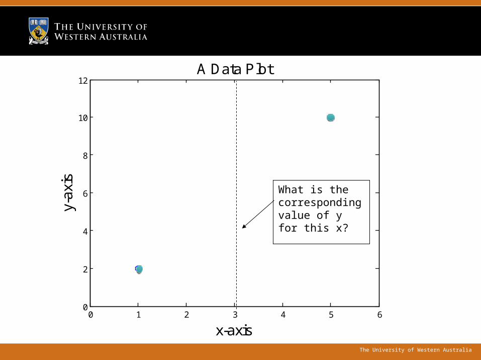
Interpolation◊ When you take data, how do you predict what other data

points might be?

◊ Two techniques are :

• Linear Interpolation

– Assume data follows a straight line between adjacent measurements

• Cubic Spline Interpolation

– Fit a piecewise 3rd degree polynomial to the data points to give a “smooth” curve to describe the data.


0 1 2 3 4 5 60

2

4

6

8

10

12A Data Plot

x-axis

y-ax

is

What is the corresponding value of y for this x?


Linear Interpolation

◊ Assume the function between two points is a straight line

How do you find a point in between?

X=2, Y=?


0 1 2 3 4 5 60

2

4

6

8

10

12A Data Plot

x-axis

y-ax

is

-1 0 1 2 3 4 5 6

0

2

4

6

8

10

12

14

16Measured Data

x-axis

y-ax

isInterpolated Point

Interpolated Points

Linear Interpolation – Connect the points with a straight line to find y


MATLAB Code

◊ interp1 is the MATLAB function for linear interpolation

◊ First define an array of x and y

◊ Now define a new x array, that includes the x values for which you want to find y values

◊ new_y=interp1(x,y,x_new)

◊ Exercise: How would you implement the interp1 function yourself? What control structures would you use?


-1 0 1 2 3 4 5 6

0

2

4

6

8

10

12

14

16Measured Data

x-axis

y-ax

is



-1 0 1 2 3 4 5 6

0

2

4

6

8

10

12

14

16

x-axis

y-ax

is

Measured and Interpolated Data

Both measured data points and interpolated data were plotted on the same graph. The original points were modified in the interactive plotting function to make them solid circles.


Cubic Spline

Cubic Spline Interpolation◊ A cubic spline creates a smooth curve, using a third degree

polynomial.◊ The curve does not correspond to a single cubic. Instead it is a set

of cubic polynomials that meet at the measured data points.◊ In fact, the polynomials are continuous up to their 2nd derivative.◊ Finding these polynomials can be reduced to the problem of solving

a set of simultaneous linear equations, (but this is beyond the scope of this unit).

◊ Note, that all the original points remain on the curve.


We can get an improved estimate by using the spline interpolation technique



-1 0 1 2 3 4 5 6

0

2

4

6

8

10

12

14

16Cubic Spline Interpolation

x-axis

y-ax

is

Cubic Spline Interpolation. The data points on the smooth curve were calculated. The data points on the straight line segments were measured. Note that every measured point also falls on the curved line.


Other Interpolation Techniques

◊ MATLAB includes other interpolation techniques including

• Nearest Neighbor

• Cubic

• Two dimensional

• Three dimensional

◊ Use the help function to find out more if you are interested


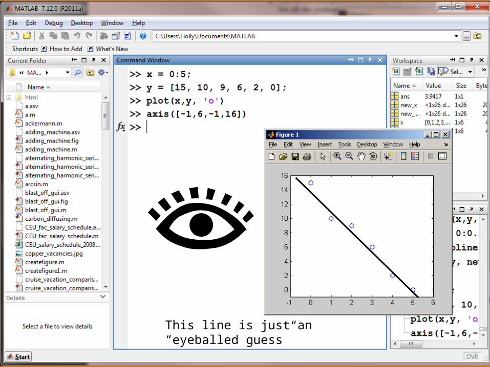
Curve Fitting ◊ There is scatter in all collected data.

◊ We can estimate the equation that represents the data by “eyeballing” a graph.

◊ There will be points that do not fall on the line we estimate.

◊ Curve fitting is used when we want to match an analytical (or symbolic) model to a set of measurements which may contain some error.

◊ Interpolation is used when we assume that all data points are accurate and we would like to infer new intermediate data points.


This line is just an “eyeballed guess”


Least Squares

◊ Finds the “best fit” straight line

◊ Minimizes the amount each point is away from the line

◊ It’s possible none of the points will fall on the line

◊ Linear Regression is used to define the line that minimizes the square of the errors (the distance each point is from the value predicted by the line).

◊ The same method is used by the slope function in Excel.


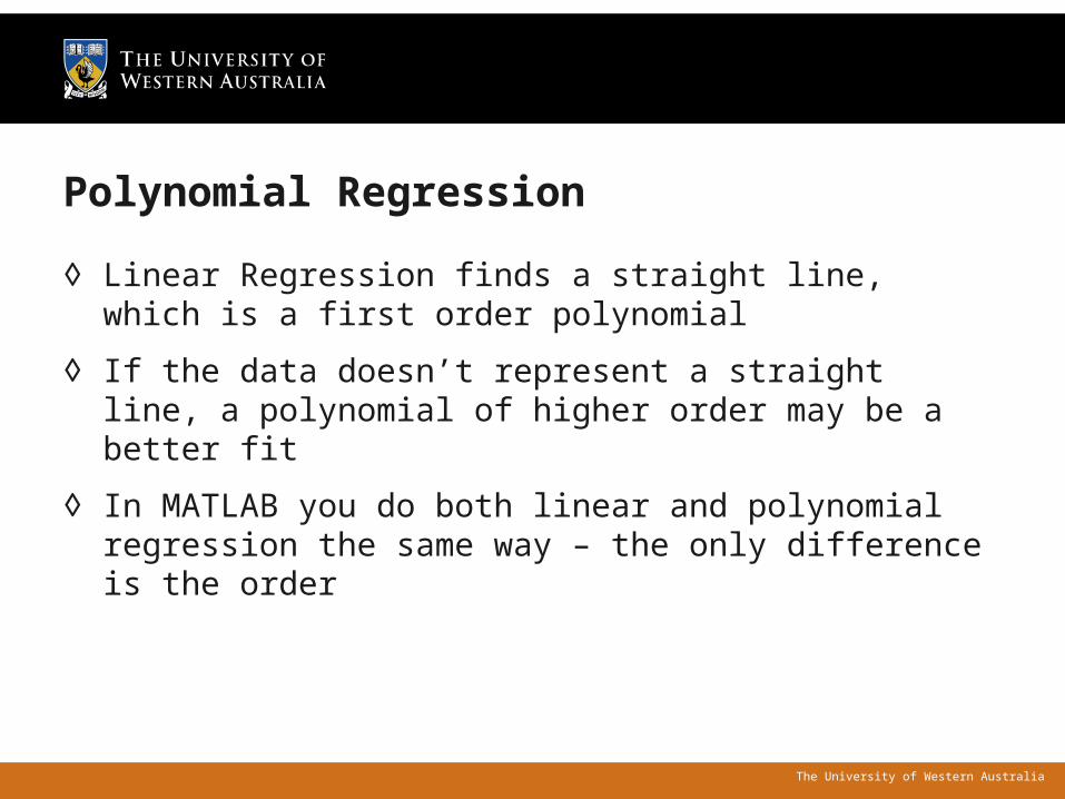
Polynomial Regression

◊ Linear Regression finds a straight line, which is a first order polynomial

◊ If the data doesn’t represent a straight line, a polynomial of higher order may be a better fit

◊ In MATLAB you do both linear and polynomial regression the same way – the only difference is the order


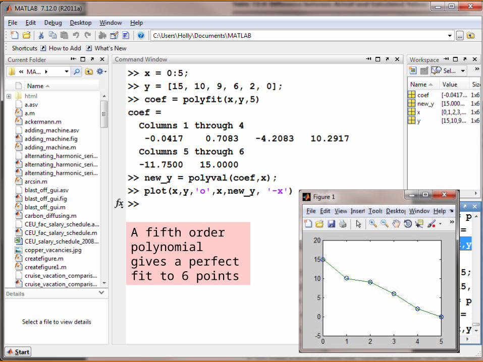
polyfit and polyval

◊ polyfit finds the coefficients of a polynomial representing the data

◊ Coef = polyfit(x,y,2); will set coef = [a,b,c] where a*x2+b*x+c is the quadratic that minimizes the square of the error.

◊ polyval uses those coefficients to find new values of y, that correspond to the known values of x

◊ newy = polyval(coef,X) will evaluate the polynomial corresponding to coef for each point in X and return the corresponding y-values. The degree of the polynomial is determined by the length of coef.


Coefficients of the first order polynomial describing the best fit line

Evaluate how close a fit you’ve achieved by taking the difference between the measured and calculated points


Least Squares Fit2( )calcy y

The polyfit function minimizes this number


Second Order Fit

20.0536* 3.1821* 14.4643y x x


A fifth order polynomial gives a perfect fit to 6 points


Improve your graph by adding more points


An example from the labs

◊ We can read in the Excel file from Lab 2 using the xlsread function:◊ data = xlsread('Rings.xls');

◊ We can extract X and Y arrays and find the line of best fit:◊ X = X(2:78);◊ Y = Y(2:78);◊ coef = polyfit(X,Y,1);◊ NewY = polyval(coef,X)



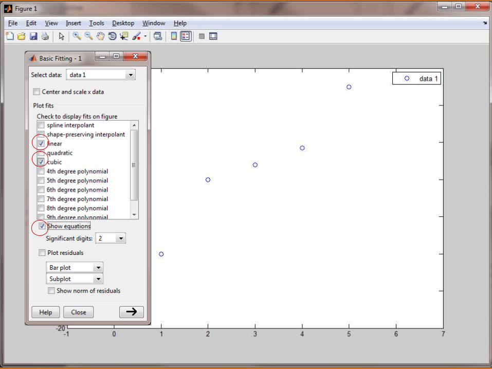
Using the Interactive Curve Fitting Tools

◊ MATLAB 7 includes new interactive plotting tools.

◊ They allow you to annotate your plots, without using the command window.

◊ They include • basic curve fitting,

• more complicated curve fitting

• statistical tools


Use the curve fitting tools…◊ Create a graph

◊ Making sure that the figure window is the active window select

• Tools-> Basic Fitting

• The basic fitting window will open on top of the plot




Plot generated using the Basic Fitting Window


Residuals are the difference between the actual and calculated data points


Basic Fitting Window


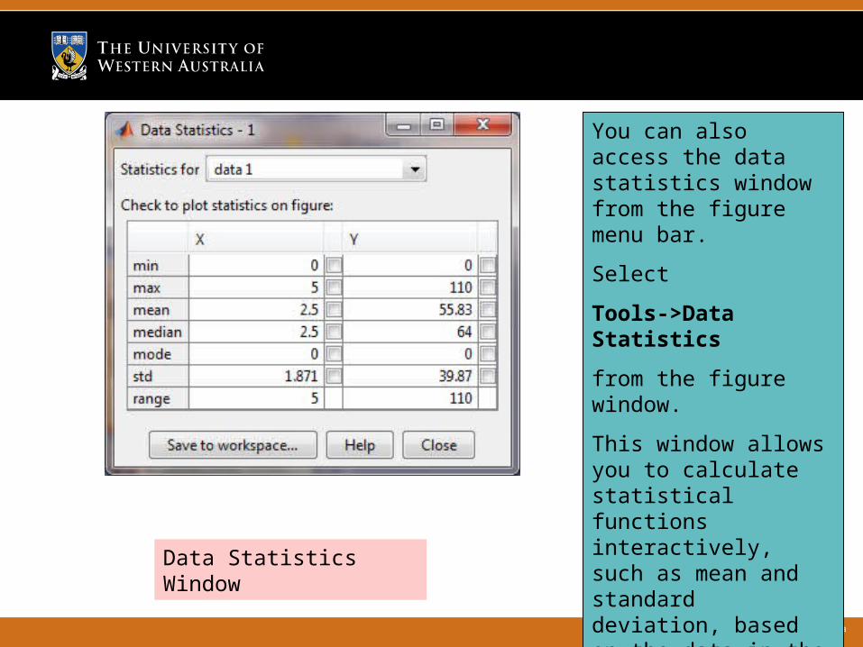
Data Statistics Window

You can also access the data statistics window from the figure menu bar.

Select

Tools->Data Statistics

from the figure window.

This window allows you to calculate statistical functions interactively, such as mean and standard deviation, based on the data in the figure, and allows you to save the results to the workspace.


Matlab Review

◊ This completes the section of the unit covering Matlab◊ There is a great deal of Matlab functionality available,

but you should be aware of the basics:• How data is represented using arrays and matrices• How variables are created and modified• How functions are defined and used• How conditions (if), loops (for, while), matrix

operations, and IO can be combined to define a process. • How to plot and visualize data.

CITS2401 Computer Analysis & Visualisation

Documents

measured data points

set of data points

interpolated data

collected data

original points

smooth curve

curve fittingmaterial

cubic spline modelsmodel