CIT - E-CDGM: An Evolutionary Call-Dependency Graph … · 2016-08-08 · 70 BULGARIAN ACADEMY OF SCIENCES CYBERNETICS AND INFORMATION TECHNOLOGIES Volume 16, No 3 Sofia 2016 Print

70

BULGARIAN ACADEMY OF SCIENCES

CYBERNETICS AND INFORMATION TECHNOLOGIES Volume 16, No 3

Sofia 2016 Print ISSN: 1311-9702; Online ISSN: 1314-4081

DOI: 10.1515/cait-2016-0035

E-CDGM: An Evolutionary Call-Dependency Graph

Modularization Approach for Software Systems

Habib Izadkhah1, Islam Elgedawy2, Ayaz Isazadeh1 1Department of Computer Science, Faculty of Mathematical Sciences, University of Tabriz, Tabriz,

Iran 2Department of Computer Engineering, Middle East Technical University, Northern Cyprus Campus,

Guzelyurt, Mersin 10, Turkey

Emails: [email protected] [email protected] [email protected]

Abstract: Lack of up-to-date software documentation hinders the software evolution

and maintenance processes, as simply the outdated software structure and code

could be easily misunderstood. One approach to overcoming such problems is

using software modularization, in which the software architecture is extracted from

the available source code; such that developers can assess the reconstructed

architecture against the required changes. Unfortunately, existing software

modularization approaches are not accurate, as they ignore polymorphic calls

among system modules. Furthermore, they are tightly coupled to the used

programming language. To overcome such problems, this paper proposes the

E-CDGM approach. E-CDGM decouples the extracted call dependency graph from

the programming language by using the proposed intermediate code language

(known as mCode). It also takes into consideration the polymorphic calls during the

call dependency graph generation. It uses a new evolutionary optimization

approach to find the best modularization option; adopting reward and penalty

functions. Finally, it uses statistical analysis to build a final consolidated

modularization model using different generated modularization solutions.

Experimental results show that the proposed E-CDGM approach provides more

accurate results when compared against existing well-known modularization

approaches.

Keywords: E-CDGM, call-dependency graph, software architecture,

modularization, evolutionary approach.

1. Introduction

Software architecture provides developers with the higher-level structural

information necessary for comprehending software systems, as the architecture

model provides information about the system components, as well as their

71

interconnections and interfaces [1]. During the software maintenance and evolution

processes, the actual software architecture could deviate from the originally

documented architecture. Such architecture changes are not necessarily well

documented, and in some extreme cases are not documented at all, as in legacy

software systems. This of course leads to software miscomprehension, which

hinders the software future evolution and maintenance processes. Hence, developers

who want to understand the system opt to manually study the source code to re-

create the system architecture. Of course, the manual approach does not work when

the software system is quite big and has complex relationships between its modules.

Hence, numerous attempts have been continuously made to design automated or

semi-automated software architecture extraction tools [2]. Such automated approach

for software architecture extraction is known as software modularization, which is a

key activity in the reverse engineering process adopted to improve software

understanding and maintenance [3-5]. The goal of the software modularization

process is to automatically partition the classes of a software system into modules

(or subsystems, i.e., a number of interrelated classes), such that the connections

between the classes of different modules (called coupling) are minimized, and the

connections between the classes of the same module (called cohesion) are

maximized. In general, low coupling and high cohesion are famous characteristics

for well-designed software systems [6, 7], as they have a significant impact on

critical software quality attributes such as reliability, portability, reusability,

operability, flexibility, testability and maintainability [2].

The first step in the software modularization process is to extract a Call

Dependency Graph (CDG) from the source code. A CDG indicates the method

invocations between software’s classes, details are given in Section 2. This step

should take into consideration different relation types between classes such as

method-to-method calls, class-in-method definitions, aggregation, namespace,

polymorphic calls and static classes. After the CDG extraction, it should be

modularized to extract the appropriate architecture. Unfortunately, existing

approaches for CDG generation such as [1, 8] are pessimistic, that they tend to

generate big sizes CDGs regardless of the required design semantics, which of

course have a negative impact on the quality of the resulting modularization.

Nevertheless, they ignore important design aspects such as polymorphic calls.

Furthermore, they are tightly coupled to the used programming language. To

overcome these problems, this paper proposes the E-CDGM (Evolutionary Call

Dependency Graph Modularization) approach. E-CDGM extracts the CDG from the

given source code, and decouples the extracted CDG from the programming

language by using the proposed intermediate code language (known as mCode).

This intermediate code language converts the source code of any language into

mCode; removing any unnecessary details. The generated mCode is used to

generate the CDG; taking into consideration method-method calls, class-method

definitions, aggregation, namespace, polymorphic calls and static classes, details are

given in Section 4. The E-CDGM approach uses a new evolutionary optimization

approach to find the best modularization option; adopting both reward and penalty

functions, which increases the speed of the modularization process. Finally, it uses

72

statistical analysis to build a final consolidated modularization model from different

optimized generated modularization solutions. Experimental results show that the

proposed E-CDGM approach provides more accurate results when compared

against existing well-known modularization approaches.

The rest of the paper is organized as follows. Section 2 provides the

background information required for CDG extraction, and addresses the limitations

of the existing works. Section 3 discusses the proposed intermediate code language

and its semantics, While Section 4 explains the proposed algorithm for CDG

extraction. Section 5 proposes the new evolutionary approach for CDG

modularization, while Section 6 provides the statistical analysis approach used to

build the final consolidated modularization model. Section 7 provides the E-CDGM

evaluation experiments. Finally, Section 8 concludes the paper.

2. Background and related work

This section provides the basic information required for CDG extraction. The main

aim of the CDG is to provide an abstract view of software system structure [1]. A

CDG indicates the method invocations between software’s classes. For example,

consider the following sample code:

class B{ Public A o;

Public void m1(){o.m(); };

}

In this code, a call like o.m() inside class B, in which “o” is an object of class

A clearly creates a dependency between the two classes A and B, through a method

in class B.

Let {N1, N2, …, N8} denotes a software system including eight classes; Fig. 1

shows a sample CDG this software system.

N1

N3

N2

N4

N6

N5

N7 N8

C6

C5

C7

C3

C4

Fig. 1. A sample call dependency graph

In object oriented programming languages, each node of the CDG represents a

class and the edges represent a method call between two classes of the source code,

i.e., if node 1 and node 2 show class 1 and class 2 respectively, the edge between

them represents a method call, i.e., in the Class 1, a (public) method of Class 2 is

73

called. In a CDG, there can also be weighted edges. This way, the weight of an edge

indicates the number of relationships between classes.

Currently, there are many tools for CDG extraction such as Acacia (for C++

programs) [9], Columbus (for C++ programs) [8], Chava (for Java programs) [10],

NDepend (www.ndepend.com; for most object oriented programs), Understand

(www.scitools.com; for most object oriented programs), Bauhaus (for most object

oriented programs) [11], DPMld (for .Net platform) [12] Reveal (for C++ programs)

[13] and Imagix-4D (www.imagix.com; for most object oriented programs).

Unfortunately, these tools are tightly coupled to the adopted programming

language, furthermore they (excluding DPMld) identify only inheritance,

aggregation, and instantiation relationships, and totally ignores the polymorphic

calls when creating CDGs. To show such limitation, let us consider the pseudo

codes in Figs 2 and 3. Code in Fig. 2 does not include polymorphic call, while code

in Fig. 3 does.

Fig. 2. A pseudo code without polymorphic call Fig. 3. A pseudo code includes a

polymorphic call

In Fig. 2, the declared type for variable “a” is class “A” and “a” instantiated of

class “A”. Thus call destination a.method1( ) is considered class “A”. While in

Fig. 3, in class “C”, the declared type of “a” is class A but “a” instantiated of class

“B”. Thus, call destination a.method1( ) should be considered class “B” not class

“A”. This kind of call is called polymorphic call. Fig. 4 shows CDG generated for

Fig. 3 by existing Chava, NDepend and Understand tools, while the appropriate

CDG for Fig. 3 is shown in Fig. 5. Existing tools construct the call graph

pessimistically that they conservatively do not eliminate any probable call from the

graph. As a result, the obtained call graph will have so many edges and a negative

impact on the modularization result, as the computation of coupling and cohesion

metrics will not be precise. In such cases, existing tools consider both classes as call

destination.

Class A { Public void method1 ( ){ print (“This is A”);}

}

Class B extends A { Public void method1 ( ){ print (“This is B”);}

}

Class C extends A { Public void method1 ( ){ print (“This is C”);}

}

Class Main { Public void method2 ( ){

A a;

a=new A (); a.method1 ();

}

}

class A {…. } class B extends A {…. }

class C{

public void m1(){ A a

a=new B();

a. method1(); }

}//class c

class main_Class{ public void main(){

A a=new A();

a. m();

C c=new C(); c. m1();

}//main

}//main_class

74

Modularization of a software system is NP hard problem, particularly if input

state space is very large. Hence, heuristic techniques such as genetic algorithm are

adopted for finding the optimal or near optimal answer during a reasonable time

such as the works in [14-22]. Genetic modularization algorithms are very subjective

[1, 17], and adopted by well-known tools such as Bunch [1], Dagc [17] and Craft

[18]. Bunch is a well-known tool for software modularization, and widely used in

industry. Efficient behaviour of a genetic algorithm depends on proper design of

encoding. One of the disadvantages of the Bunch algorithm is the largeness of

search space due to presence of some repetitive answers, i.e., generated codes that

have apparently different representations, but in reality, they represent the same

partition. Search space in Bunch algorithm and some existing algorithms is nn; this

large search space decelerates speed of this algorithm to find appropriate

architecture. E-CDGM overcomes such problem by using reward and penalty

functions, and by building a consolidated model from different modularization

answers appeared in the search space. Bunch and CRAFT algorithms use Acacia

and Chava algorithms to construct CDG. Therefore, these tools are tightly coupled

to C++ and java programming languages. Also, DAGC algorithm use FRTA

algorithm to construct CDG, which is tightly coupled to the java programming

language; therefore, other programming languages cannot use DAGC features.

E-CDGM overcomes this problem by using the intermediate code language mCode

to generate the CDGs.

4. The proposed intermediate code language (mCode)

The purpose of the intermediate code language is to decouple the CDG extraction

process from the adopted programming language. Hence, the source code written in

any language will be converted into the intermediate code language known as the

mCode, where the generated intermediate code consists of information extracted

from the source code that will be used as an abstract model for CDG extraction. To

achieve such goal, the lexical structure of the programming language as well as the

source code will be given as inputs to the mCode convertor. Fig. 6 shows the

adopted conversion process.

The Flex complier is a tool that automatically generates the lexical analyzer.

This tool takes the lexical specification of source language then produces the related

Fig. 4. CDG generated for Fig. 3 by Chava, NDepend,

Understand, and Bauhaus algorithms Fig. 5. Appropriate CDG for Fig. 3

75

lexical analyser, which will take the source code as input to automatically generate

the intermediate code. The programming language lexical specifications are

manually constructed according to the proposed intermediate code semantics shown

in Table 1. It is important to note that the programming language lexical

specifications are defined only once, and it will be used later for any java programs

to convert them into mCode.

Fig. 6. Generation steps of intermediate code

Every intermediate code is described, based on a meta-model that indicates

some facts that should be extracted from the source code. This meta-model is

extracted and saved in a descriptive language named mCode. According to the

meta-model in Table 1, the extracted intermediate-model includes class, interface,

attributes of class, method of class, parameters of methods, inheritance relation,

abstract, the relation of instantiated a class, call and access to attribute of a class. In

Table 1, the command structures in mCode have the format: Opcode par1, par2,…,

parn, where Opcode represents one of the programming language contexts (i.e.,

commands and keywords), and pari represents an attribute describing the involved

context. For example, in java source code, the context of “Class” can be an Opcode

and its describing attributes are class name, namespace. Hence, this command in

our intermediate model is written as: Class namespace, class name. Table 1 shows

the mCode Opcodes and their parameters.

Table 1. Opcode formats in mCode Comment Description Intermediate code opcode

Type: abstract, interface, static, sealed, …

Define a class in a specific namespace (or package in java)

Class {namespace.}[ClassName]{:Type}

Define a struct in a specific

namespace Struct {namespace.}[StructName]

Block type indicate the Namespace, Struct or Class

Begin of BlockType Begin [BlockType]

End of BlockType End [BlockType]

Access type can be as public, protected or private

Identify the class inherited from Inherits {namespace.}[ClassName]{ :

AccessType }

Class include field of other class as

ClassName

Field [FieldName]:{namespace.}[ClassName

]

Type: static, … Identify a method within a class Method [MethodName]{:Type}

Identify parameters of a method Parameters

[name]:{namespace.}[ClassName]

Identify the return value of a class

that are as class Returns {namespace.}[ClassName]

Identify call variable (object) Call

{namespace.}{ClassName.}[Name]

Define a variable type of

ClassName Var

[VarName]:{namespace.}[ClassName]

Type: static, … Property of type of VarType Property

[PropertyName:VarType]{:Type}

Flex

Compiler Programming Language

Lexical Specifications

Lexical

Analyzer

Program in mCode

Program Source Code

76

Fig. 7 shows the lexical specification for the java programming language using

the proposed mCode semantics. This lexical specification is used to generate the

mCode for any java program. For example, the source code given in Fig. 8 will be

converted into the mCode depicted in Fig. 9.

package<packageName> { [public|private] [static] interface <interfaceName> { action: write ("class"+<packageName.>+ "interface"+<interfaceName>); action: write ("Begin Interface"); [public [static] <dataType><methodName>([<dataType><parameterName>]*); action: write ("method"+ <methodName>); action: write ("Returns"+ <parameterName>); action: write ("endMethod"+ <methodName>); ]* } action: write ("end interface"); [public|private] [static] abstract <abstractName> { action: write ("class"+<packageName.>+ "abstract"+<abstractName>); action: write ("Begin Abstract"); [ public [static] <dataType><methodName>([<dataType><parameterName>]*); action: write ("method"+ <methodName>); action: write ("endMethod"+ <methodName>); ]* } action: write ("end abstract"); [public|private] [static] class <className> { action: write ("class"+<packageName.>+ <className>); action: write ("Begin class"); [ extend <className>action:write ("inherits"+ <className>); [,<className>action:write ("inherits"+ <className>);]* ] [implement <implementName>action:write ("implement"+ <implementName>);] [public|private] <className><objectName>action:write ("type"+ <className>); [,<className><objectName>action:write ("type"+ <className>);]* [ [public|private] [static] <dataType><methodName>([<dataType><parameterName>]*); { action: write ("method"+ <packageName.> + <methodName>); [<className><objectName>=new <className>([parameterName]*) action: write ("createObject"+ <className>); ]* [ <objectName> . <functionName>([<parameterName>]*); action: write("call" +<packageName.><methodName> + "class" + <className>) ]* } action: write ("endMethod" + <methodName>); ]* } action: write ("endClass" ); } action: write ("endnamespaceName" + <packageName>);

Fig. 7. Java lexical specification using mCode

Fig. 8. A sample source code Fig. 9. The generated intermediate code for Fig. 8

Class NS1 B Begin class Inherits className1 // inherits class B from Inherits className2 // inherits class B from Type TA // a variable of class A in classB Type TC// a variable of class C in class B Method m // a method named B in class B Begin method Call TA EndMethod m //end of method EndClass B //end of class endNamespace NS1 // end of name space

package NS1

{

class B extends className1 , className2

{ TA a; TC f;

public m( )

{a = new TA( ); }

}

77

5. The proposed CDG extraction approach

In this section, we propose a new algorithm to generate CDG from the intermediate

code considering the type of relation between classes such as, method-method,

class-method, aggregation, namespace, polymorphic calls and static class. In

general, classes are related with each of the following two ways.

1. Interaction Type. Determines ways in which the two classes communicate

with each other.

Aggregation: are of the form class-attribute as a class D is the field of class

M.

Class-method: in this case, class D is the type of a parameter of method mC

of a class C, or if a class D is the return type of method mC.

Method-method: in this case, method mD of a class D directly invokes a

method mC of a class C, or a method mD receives via parameter a pointer to mC

thereby invoking mC indirectly

2. Relation Type. Determines ways in which the two classes are related to

each other.

Inheritance: in this case, class D inherits attribute and behaviour of class C

or vice versa.

Friendship: in this case, a friend class to have access to the private and

protected members of the class.

Other relations between classes C and D are interface and abstract.

Variable Type Analysis (VTA) [23] algorithm is a well-known algorithm for

determining destination of a call that is used in compiler construction. We recast it

for constructing CDG in software modularization domain. In this section, we extend

VTA to support static classes and name spaces, and then we explain how to

construct precise CDG from the generated intermediate code (including explicit and

polymorphic calls). The aim of the enhanced VTA is to precisely determine a call’s

destination.

Definition 1. Destination of a call such as o.m(), in this algorithm showed as

Destination(o), it is identified as follows:

a) If call of o has a declared class type C, the possible run-time of o,

Destination(o), includes C and all sub-classes of C.

b) If call of o has a declared interface I, the possible run-time of o,

Destination(o), includes: (1) the set of all classes that implement I or implement a

sub interface of I, which we call implements(I); (2) all subclasses of implements(I).

The main aim is to identify a set of reaching variable to o in each call likes

o.m( ) precisely. This set, called Receiving-types(o). The proposed algorithm uses a

graph to perform this action. For example, we say type A reaches to variable o if

once at least there would be one path in the program run to be started by object of

type A (e.g., as v=new A( )), and then chain of assignment would be as follows:

(1) x1 = v, x2 = x1, …, xn= xn-1, o = xn.

Each one of the assignments would be a call or return value of a method.

Given a program mCode, CDG is constructed using algorithm 1 (i.e., the enhanced

VTA algorithm). The algorithm has five main steps. The first step is about

78

constructing the CDG graph using the variables and the assignments. The second

step is about revising the graph based on the inheritance relations. The third step is

about removing cycles from the graph. The forth step is about computing the

possible receiving nodes for each call to check type propagations. Finally, the fifth

step is about determining the actual destination of each call.

In Fig. 10a we give the important parts of an example program. Fig. 10b to

Fig. 10e show above Steps 1-4 of Algorithm 1 for code in Fig 10a. Fig. 10b shows

construction of the graph based on assignments in code. That in the source code if

we have a1=a2, in this case, in the constructed graph, we will an edge from a2 to a1

and so on. Fig. 10c shows the instantiated class of variables (i.e., the initial assigned

values), for example, in Fig. 10a, we have a1= new A(); therefore, in the Fig. 10c

the label of a1 is {A}, and we have b1=new B() then the label of b1 is {B} and so

on. Fig. 10d shows removal of cycles from graph that if some of variables are

located in cycle, and they have no type, in this case we consider them as a node.

Fig. 10e shows propagation of types. As nodes a3 and b3 are in a cycle, hence they

are converted to a united node before propagation. After calculating Receiving-

types (o) set for each call using Algorithm 1, the actual destination of each call is

determined using Equation 2.

Algorithm 1. Enhanced VTA for determining actual destination of a call

Input: The program mCode

Output: The extracted CDG

Step 1. Graph Construction, in which nodes show variables and each edge as

a→b shows an assignment as b=a.

Step 1.1. Nodes are created as follows:

1) for each field f (where f has a reference to a class) in class C into

namespace NS, creates a new node labelled with NS.C.f

// This condition occurs when a class is defined as static class or occurs

aggregation

2) for each method m in class C into namespace NS, creates a new node

labelled NS.C.m

Step 1.2. Edges are added as follows:

For each statement of form lhs=rhs; or lhs=(C) rhs; where lhs and rhs must be

an ordinary, field or array reference, we add a directed edge from the rhs node to

the lhs node.

Step 2. Initialized graph, in which all assignment would be searched as

lhs=new type and type would be placed as initial value in Receiving-types(lhs) set.

Step 3. Remove all cycles from the graph and generate a new directed graph

without cycles. To remove cycles, the nodes those are located in a cycle to be

converted into a node. Receiving-types (lhs) of this node would be obtained from

the union of nodes.

Step 4. Compute the Receiving-types(o) set for each call through propagation

of types in the graph.

Step 5. After above works, actual destination of each call, EIMA(o), would be

obtained by following relation:

(2) EIMA(o)= Destination(o) ∩ Receiving-types(o).

79

Fig. 10. Computing the Receiving-types(o) set for each call

6. The proposed CDG modularization approach

The general problem of graph partitioning (of which software modularizing is a

special case) is NP-hard [1]. Therefore, to reduce the time complexity to a

polynomial upper bound, most researchers using heuristic based algorithms for

software modularizing. In this section, we propose a new evolutionary algorithm to

modularize software systems. First, we will discuss the proposed encoding scheme,

and then go on to discuss the used fitness, reward, and penalty functions. Finally,

we discussed the proposed evolutionary algorithm for CDG modularization.

6.1. The proposed modularization encoding approach

Each modularization solution is encoded as a vector (i.e., a learning automaton) and

each vector represents a permutation of nodes of the CDG. The number of vector

cells is the number of CDG classes. Each vector cell includes four rows, where the

first row is the class number (i.e., m), the second row is the partner number of a

class (i.e., p), the third row is the depth of cell vector (this required in learning) and

the fourth row is the selection probability of each class for penalty or reward. The

initial selection probabilities for the classes are equal (as shown in Fig. 11). Each

vector’s cell is called an action. The partner number of a class is any class number

in the CDG that has the potential to be included with the class number m in the

same module. The partner number is determined according to the numbering

method proposed in [17], in which if the partner number p for class m be equal or

greater than m, then m is placed in a new module; otherwise m belongs to the same

80

module that p is allocated in that. Once the partners of every cell are defined,

modules could be determined by grouping all related partners into the same module.

For example, Fig. 11 shows a given CDG and its corresponding vector structure. As

we have 6 classes, then we will have 6 cells, every cell is assigned a partner, for

instance the partner for class 2 is class 5, and the partner for class 3 is class 6, while

class 1 has no partners in this case it is assigned to itself. Once the partners’

allocation is finalized, we can see we can partition the CDG into three modules,

module 1 has only class 1, while module 2 has classes 2 and 5, and finally module 3

has classes 3, 4, and 6.

This efficient encoding reduces number of permutations from nn to n!. This

reduction in size of search space would result in faster convergence of the

algorithm.

Class number

(m)

1 2 3 4 5 6

P 1 5 6 3 2 4

Depth 0 0 0 0 0 0

Probability 0.16 0.16 0.16 0.16 0.16 0.16

Fig. 11. A CDG partition and its corresponding Vector structure

A vector is defined as tuple },,,,,,{ TPFva in which:

},...,{ 1 raaa is a set of vector’s actions (r is number of the software

classes)

},...,{ 1 rvvv is a set of used objects in the vector. These objects do not

include module number of graph nodes; they are other node numbers of graph.

These objects moving in various situations of vector and produce different

permutation (objects are shown in Fig. 11 by the name of p.)

},...,{ 1 r is the result of evaluation of a selected action. If 0i , i.e.,

selected action meets the desired criteria, it should be rewarded. If 1i , i.e.,

selected action does not meet the desired criteria, it should be penalized.

RN ,...,, 21 is set of situations; N is the number of states an action can

go through to decide a mutation is needed or not; R is the number of vector actions.

81

:F is mapping method of situations. This method determines

the next situation from value and current situation.

},...,{ 1 rppP is probabilities array. This array shows selection probability

of each action and then upon either rewarding or penalty would change after each

selection. For action i, the action probability is

(3) 1

( ) ,iP tr

i 1, 2,..., r (r is the number of classes);

)](),(),([ npnnaTT is learning algorithm (described in Section 6.4).

6.2. The adopted vector fitness function

Quality function is used to determine the fitness degree of each vector in

population. Our aim to modularize is to increase cohesion and decrease coupling of

modules as much as possible. Thus, we adapt quality function presented in [1] to

consider the cases mentioned earlier. Suppose:

C1= class-attribute and |C1|= number of class-attributes in the source code,

w1= weight of C1

C2= class-method and |C2|= number of class-methods in the source code,

w2= weight of C2

C3= method-method and |C3|= number of method-methods in the source code,

w3= weight of C3

We define the quality function for each generated module as follows:

(4)

3

1

3 3 #modules

, ,

1 1 1,

2( | |)

MF ,

2( | |) ( (| | | |))

i i

im

i i k i j j i

i k j j i

w C

w C w C C

1 number of modules in a vector,m

|Ci,j| represents the call numbers from module i to module j and |Cj,i| represents the

call numbers from module j to module i. For module m ( km 1 ), where k is the

number of modules, the Module Factor, MFm, is a normalized ratio between the

total weight of the internal edges (edges within the module) and half of the total

weight of external edges (edges that exit or enter the module). The Modularization

Quality (MQ) for a CDG partitioned into k modules is calculated by summing the

Module Factor (MF) for each module:

(5)

1

MQ MF .k

m

m

6.3. The proposed reward and penalty functions

The evolutionary process of proposed algorithm is accelerated using learning. In the

proposed algorithm, the learning is done using reward and penalty functions. For

this purpose, beside evaluation of vectors, the actions are evaluated based on its

effect on vector value. So, the most proper location for actions inside vectors is

gradually determined during the evolutionary process. Generally, penalty and

reward are applied in the proposed algorithm in this manner: During modularization

82

process, the algorithm selects action ia in a vector and evaluates it, if it receives

favourable response (i = 0), probability (Pi(n)) related to this action would increase

and probability of other actions would decrease. If it receives an unfavourable

response (i = 1), Pi(n) related to this action would decrease and the probability of

other actions would increase. In this paper, we use the linear learning scheme

proposed in [24], which computes the linear learning scheme for multiple actions as

follows:

(6) f p n ap nj j j( ) ( )

, 0 1 a ,

(7) g pb

rbpj j n j n( ) ( )

1.

Functions gj and fj are non-negative functions, which are called reward and

penalty functions, respectively. In above equations r, a, and b are respectively

number of actions in a vector, reward and penalty parameters. We can control rate

of convergence of a vector by setting a and b parameters. In the Equations (6) and

(7), the learning algorithm is known as linear reward penalty if a and b are equal. If

b is much smaller than a, the learning algorithm is known as linear reward epsilon

penalty. Penalized and reward probability functions in linear learning algorithms are

defined as follows:

For a favourable response i:

(8)

( 1) ( ) [ ( )] , ,j j j jp n p n f p n j j i ,

but

f p n ap nj j j ; so, 1 1 ,j j j jp n p n ap n a p n

and

(9)

1, 1

1r

i i j j

j j

p n p n f p n

p n ap ni j

j j i1,

p n a p ni j p n a p ni i1 .

Unfavourable response i:

(10) npgnpnp jjjj 1 ,

but

,1

j j jb

g p n bp nr

so

p n p nb

rbp nj j j

1

1 1 ,

1j

bb p n

r

and

(11)

r

ijj

jjii npgnpnp,1

1 =

p n

b

rbp ni j

1 p n b b p ni j p n b b p ni i1 =

p n b b bp ni i 1 b p ni , 0 1 b .

83

Algorithm 2. Evaluation of an action of a vector for doing reward and

penalty Step 1. Select an action of a vector according to its probability (Equations (8)-

(11))

// an action of a vector indicates a vertex in CDG

Step 2. Compute vertex cohesion

//Vertex cohesion is the ratio of number of vertices connected to vertex “u”

inside the module containing this vertex to the total number of intra-connections

this module //

Step 3. Compute vertex coupling

//Vertex coupling is the ratio of number of inter-connections vertices

connected to vertex u to the total number of inter-connections vertices possible to

be connected to this module//

Step 4. If (vertex cohesion – vertex coupling > MQ

K)

//where K represents number of modules in vector and MQ is defined in

Equation (5)

Step 4.1. The vertex will be rewarded

Step 5. Else

Step 5.1. The vertex is penalized // the modularization is not appropriate

The main aim of these probabilities is to use previous behaviour of the system

in order to take decisions for the future, hence, learning occurs. In each repetition of

the evolutionary modularization algorithm, an action of each vector would be

selected according to its probability (as in Equations (8)-(11) and this action can be

evaluated as in Algorithm 2.

The modularization algorithm selects an action ia in a vector based on its

probability (Equations (8)-(11) and evaluates it (Algorithm 2). If number of

unfavourable responses of an action were more than number of favourable

responses, this action would be replaced by another action to generate a new

permutation.

6.4. The proposed evolutionary modularization algorithm

The modularization algorithm takes the following inputs:

1) The number of vectors to be generated |V|. It is the number of possible

modularization solutions to be generated at a given time.

2) The vectors maximum depth N. It represents the number of states an

action can go through to decide its mutation. It can be seen as the number of

internal states an action can go through during the learning process.

3) The number of generations to be done G. Any generated vector could be

mutated to search for better solutions, however to avoid having an infinite number

of mutation, we specify a maximum number of generations a vector can go through.

Based on the given number of vectors, several vectors are generated randomly.

The algorithm performs following steps on all vectors until the given number of

generations is reached. The modularization algorithm selects an action ai in a vector

84

based on its probability, and then evaluates it as in Algorithm 2. Based on the

evaluation results, it will decide to keep the action in its place in the modularization

solution, or change its place to find a better modularization solution (i.e., perform a

mutation operation). The decision of an action mutation is decided based on the

internal state the action has, as we do not want to perform a mutation step every

time an action is penalized. To explain this idea let us assume a vector includes R

actions ( Raaaa ,...,,, 321) and has RN internal state ( RN ,...,, 21 ). Internal

states of N ,...,, 21 are related to a1; NNN 221 ,...,, are related to a2, and

RNNRNR ,...,, 2)1(1)1( are related to aR; 1 represents the deepest state for a1;

and N is the most shallow state for a1, similarly 1N

represents the deepest state

for a2, and N2 is the most shallow state for a2, and so on. For example, if we let

N=5, it means that each state machine has 5 states, so 5 (i.e., the shallowest state) to

1 (i.e., the deepest state) for action 1, while states 10 (i.e., the shallowest state) to 6

(i.e., the deepest state) are for action 2. Hence, N is border-state of the first action

and 2N is border-state of the second action, and so on. Every action will start at a

given state, and it will move inwards towards deeper states if it is rewarded, and it

will move outwards towards shallower state if it is penalized. If an action reaches a

border-state and receives undesirable response, it would be displaced by another

action in the vector, in other words, a mutation is need and a new permutation of

classes and modules would be generated. Jumping between actions, means moving

from the shallowest of the penalized action, to the shallowest state of the next

action. The algorithm searches for an action in the vector for displacement so that

MQ value in that permutation is more than others. If MQ value of new permutations

generated is lower than initial permutation, it remains the same initial permutation.

The proposed modularization algorithm is shown in Algorithm 3.

Algorithm 3. CDG modularizations Input:

- The number of vectors to be generated |V|

- The maximum depth for vectors N

- The number of generations G

Output: A vector with the best possible fitness

BEGIN

// initialize selection probabilities

for i=1 to |V| do

for j=1 to number of classes do

rtP ji

1)(, // r is number of classes

// Find Solutions

Repeat the following until G is reached for every vector

{

for i=1 to |V| do // size of population

begin

85

- Select Actionu of the Vectori with probability Pi(t)

- IF MQ

( ) ( )u uvertexCohesion Action vertexCoupling Actionk

THEN

// k is the number of modules

begin

- reward(Actionu); // Make inwards to a deeper state

-Update its probability using Equations (8) and (9)

end;

ELSE

begin

If (Actionu is in border-state and It is Penalized)

for i=1 to number of actions in vectori do

begin

Actionu would be displaced randomly with ActionT in vectori

Produce a new permutation as vectorj

(MQ(vector ) MQ(vector ))j iif

Accept a new permutation and return the new permutation

// return the new vector

Else

vectori remains in the same previous permutation

end;

Else

begin Penalize(u); // move outwards to a shallower state

Update its probability using Equations (10) and (11)

end;

end; // ELSE

end;// for

}

END.

7. The proposed modularization consolidation approach

Due to the heuristic nature of proposed algorithm in Section 6, it may produce

results with the same quality but different modularization for different runs on a

given graph. In different modularization solutions, it is observed regular

displacement of several classes between different modules, while other classes

displace less. Hence, we believe the common patterns between the obtained

solutions should appear in the final solution. To achieve this aim, we calculate the

percentage that two different classes are placed in the same module in different

obtained modularizations, then using statistical analysis to decide if they should

appear together in the final solution or not. The statistical analysis is done as

follows.

86

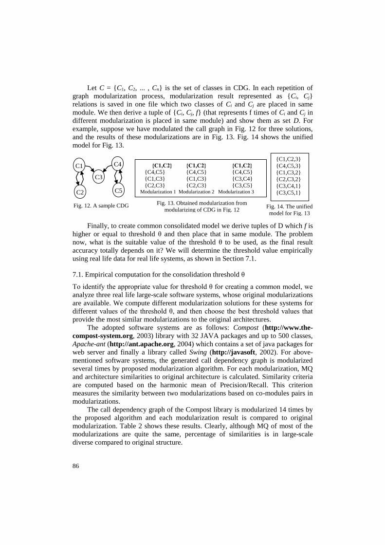
Let C = {C1, C2, ... , Cn} is the set of classes in CDG. In each repetition of

graph modularization process, modularization result represented as {Ci, Cj}

relations is saved in one file which two classes of Ci and Cj are placed in same

module. We then derive a tuple of {Ci, Cj, f} (that represents f times of Ci and Cj in

different modularization is placed in same module) and show them as set D. For

example, suppose we have modulated the call graph in Fig. 12 for three solutions,

and the results of these modularizations are in Fig. 13. Fig. 14 shows the unified

model for Fig. 13.

Finally, to create common consolidated model we derive tuples of D which f is

higher or equal to threshold θ and then place that in same module. The problem

now, what is the suitable value of the threshold θ to be used, as the final result

accuracy totally depends on it? We will determine the threshold value empirically

using real life data for real life systems, as shown in Section 7.1.

7.1. Empirical computation for the consolidation threshold θ

To identify the appropriate value for threshold θ for creating a common model, we

analyze three real life large-scale software systems, whose original modularizations

are available. We compute different modularization solutions for these systems for

different values of the threshold θ, and then choose the best threshold values that

provide the most similar modularizations to the original architectures.

The adopted software systems are as follows: Compost (http://www.the-

compost-system.org, 2003) library with 32 JAVA packages and up to 500 classes,

Apache-ant (http://ant.apache.org, 2004) which contains a set of java packages for

web server and finally a library called Swing (http://javasoft, 2002). For above-

mentioned software systems, the generated call dependency graph is modularized

several times by proposed modularization algorithm. For each modularization, MQ

and architecture similarities to original architecture is calculated. Similarity criteria

are computed based on the harmonic mean of Precision/Recall. This criterion

measures the similarity between two modularizations based on co-modules pairs in

modularizations.

The call dependency graph of the Compost library is modularized 14 times by

the proposed algorithm and each modularization result is compared to original

modularization. Table 2 shows these results. Clearly, although MQ of most of the

modularizations are quite the same, percentage of similarities is in large-scale

diverse compared to original structure.

C3

C4

C5

C1

C2

{C1,C2} {C1,C2} {C1,C2}

{C4,C5} {C4,C5} {C4,C5}

{C1,C3} {C1,C3} {C3,C4}

{C2,C3} {C2,C3} {C3,C5} Modularization 1 Modularization 2 Modularization 3

Fig. 13. Obtained modularization from

modularizing of CDG in Fig. 12 Fig. 14. The unified

model for Fig. 13

Fig. 12. A sample CDG

{C1,C2,3}

{C4,C5,3}

{C1,C3,2}

{C2,C3,2}

{C3,C4,1}

{C3,C5,1}

87

Table 2. Evaluating modularization results (P/R=Precision/Recall, Fm=Harmonic Mean of P/R)

Table 3 shows the abovementioned modularization results and confidence

analysis for different threshold values. Table 3 shows high percentage of

similarities of threshold value from 50 up to 60. Obviously, if we decrease threshold

value lower than 50, Fm would decrease significantly. If we increase threshold value

higher than 50, e.g., 80 and 90, we expect percentage of similarities to be higher,

but it is not, as the original architecture is not optimum (maximum cohesion and

minimum coupling).

Table 3. Variation of F for different thresholds for Compost 1 10 20 30 40 50 60 70 80 90 Threshold (θ)

2 3 3 18 41 54 54 18 20 21 Precision

74 71 69 56 22 24 44 2 1 1 Recall

3.89 5.75 5.75 27.24 28.63 33.23 48.48 3.2 1.82 1.82 Fm

To prove that the obtained threshold range provides better consolidation

quality; we computed the similarity of the consolidated model for the three above

mentioned systems using a threshold value as 60%. Table 4 shows the highest

similarity value of an obtained individual solution against the similarity of the

common model. As it was expected, the created consolidated model is the most

similar to the original architecture when compared with individual modularization

solutions for every system.

8. E-CDGM evaluation experiments

In this section, we compare the experimental results obtained of the proposed

E-CDGM algorithm and two well-known algorithms such as Bunch and DAGC.

We will use different data sets for testing these algorithms both artificial datasets

and real-life data sets. Since in Bunch and DAGC the quality of the modules is

computed by TurboMQ function [1, 18]; MQ used in this paper is different

compared to TurboMQ. In TurboMQ equation, the types of relations among classes

are not considered; in other words, if we in MQ (i.e., Equation (4)) set wi=1 and

considers the type of relation between two methods as method-method, in this case,

the MQ will be same TurboMQ, so we can use the TurboMQ to compare between

the algorithms.

Table 4. Comparison results

Model Swing Apache Compost

Highest obtained individual solution similarity 41% 35% 43%

Consolidated model similarity 61% 57% 49%

To compare E-CDGM, with Bunch and DAGC, first we tested the algorithms

using artificial data set, in which seven different CDGs with more than 200 nodes

88

are used. Each CDG was modularized twenty times. The average results are shown

in Table 5.

As we can see, E-CDGM performs the best, as it creates a consolidated model

from the different obtained solutions, while other approaches just return individual

solutions. To see if E-CDGM still performs better than other algorithms, we

compare them using real life data with characteristics shown in Table 6. Table 7

shows the final quality value of the modularization solutions obtained by E-CDGM,

DAGC, and Bunch. Results of this table is the best result among 20 times algorithm

run at the same execution time period (i.e., 100 s). As we can see in Table 7,

E-CDGM still performs better than the other algorithms for the same allowed

execution period. This confirms our claims that using a consolidated model to

generate the final solution always provides the best results.

Table 5. Comparing quality of results with TurboMQ function Modularization quality (TurboMQ)

Number of nodes 200 250 300 350 400 450 500

Bunch 6.15 6.22 7.67 8.90 5.89 6.0 6.30

DAGC 6.90 6.95 8.0 8.87 6.93 7.53 7.20

E-CDGM 7.10 7.35 9.12 9.98 7.20 8.93 9.20

Table 6. Real-life data sets and their characteristics

System description Number of relation

between modules

Number of system

modules

Software

systems

Turing compiler 32 13 Compiler

Graph design system 29 18 Boxer

Operation system 57 20 Mini tunis

Unix spell checking 103 24 Ispell

Table 7. Comparing quality of results with TurboMQ objective function E-CDGM DAGC [17] Bunch [1] Algorithm

Time, s TurboMQ

quality Time, s

TurboMQ

quality Time, s

TurboMQ

quality

Software

systems

100 1.91 100 1.65 100 1.42 Compiler

100 2.99 100 2.92 100 2.81 Boxer

100 2.49 100 2.28 100 2.21 Mini tunis

100 2.41 100 2.09 100 1.95 Ispell

9. Conclusion

In this paper, we proposed a new approach for software modularization known as

E-CDGM (Evolutionary Call Dependency Graph Modularization). E-CDGM

generates a call dependency graph from the given source code. It decouples the

extracted call dependency graph from the programming language by using the

proposed intermediate code language (known as mCode). It also takes into

consideration the polymorphic calls during the call dependency graph generation. It

uses a new evolutionary optimization approach to find the best modularization

option; adopting reward and penalty functions. Finally, it uses statistical analysis to

build a final consolidated modularization model using different generated

89

modularization options. Consolidation aggregation threshold is determined

empirically to be in the range of (0.5-0.6). Experimental results show that the

proposed E-CDGM approach provides more accurate results when compared

against existing well-known modularization approaches.

R e f e r e n c e s

1. M i t c h e l l, B. S., S. M a n c o r i d i s. On the Automatic Modularization of Software Systems

Using the Bunch Tool. – Software Engineering, IEEE Transactions On, Vol. 32, 2006, No 3,

pp. 193-208.

2. Q i f e n g, Z., Q. D e h o n g, T. Q u b o, S. L e i. Object-Oriented Software Architecture Recovery

Using a New Hybrid Clustering Algorithm. – In: 7th International Conference on Fuzzy

Systems and Knowledge Discovery (FSKD’2010), 2010, pp. 2546-2550.

3. L u n g, C., M. Z a m a n, A. N a n d i. Applications of Clustering Techniques to Software

Partitioning, Recovery and Restructuring. – Journal of Systems and Software, Vol. 73, 2004,

pp. 227-244.

4. L u n g, C., X. X u, M. Z a m a n, A. S r i n i v a s a n. Program Restructuring Using Clustering

Techniques. – The Journal of Systems and Software, Vol. 79, 2006, pp. 1261-1279.

5. B i t t e n c o u r t, R. A., G. D. D. S e r e y. Comparison of Graph Clustering Algorithms for

Recovering Software Architecture Module Views. – In: Proc. of Software Maintenance and

Reengineering (CSMR’2009), IEEE Computer Society Press, pp. 251-254.

6. P r e s s m a n, R. S. Software Engineering: A Practitioner’s Approach. Eighth Ed. 2014, McGraw-

Hill, Inc.

7. P o s h y v a n y k, D., A. M a r c u s, R. F e r e n c, T. G y i m ó t h y. Using Information Retrieval

based Coupling Measures for Impact Analysis. – Empirical Software Engineering, Vol. 14,

2009, No 1, pp. 5-32.

8. F e r e n c, R., A. B e s z e d e s, T. G y i m ó t h y. Extracting Facts with Columbus from C++ Code.

– In: Proc. of the Eighth CSMR, 2004, pp. 4-8.

9. C h e n, Y., E. G a n s n e r, E. K o u t s o f i o s. A C++ Data Model Supporting Reachability

Analysis and Dead Code Detection. – In: Proc. of 6th European Software Engineering Conf.

and 5th ACM SIGSOFT Symposioum on the Foundations of Software Engineering, 1997.

10. K o r n, J., Y. C h e n, E. K o u t s o f i o s. Chava: Reverse Engineering and Tracking of Java

Applets. – In: Proc. of Working Conf. on Reverse Engineering, 1999.

11. R a z a, A., G. V o g e l, E. P l ö d e r e d e r. Bauhaus – A Tool Suite for Program Analysis and

Reverse Engineering. – In: Reliable Software Technologies. Ada, Europe 2006, pp. 71-83.

12. Dobiš, M., L. U. Majtás. Mining Design Patterns from Existing Projects Using Static and Run-

Time Analysis. – In: Software Engineering Techniques. Berlin, Heidelberg, Springer, 2008,

pp. 62-75.

13. C l a r k e, P. J., T. H. G i b b s, B. A. M a l l o y, J. F. Power. Reveal: A Tool to Reverse Engineer

Class Diagrams. – In: Proc. of 14th International Conference on Tools Pacific: Objects for

Internet, Mobile and Embedded Applications CRPIT’2002, Sarah Matzko, pp. 13-21.

14. M k a o u e r, W., M. K e s s e n t i n i, A. S h a o u t, P. K o l i g h e u, S. B e c h i k h, K. D e b, A.

O u n i. Many-Objective Software Remodularization Using NSGA-III. – ACM Transactions

on Software Engineering and Methodology (TOSEM), Vol. 24, 2015, No 3, p. 17.

15. B a v o t a, G., F. C a r n e v a l e, A. D e L u c i a, M. D i P e n t a, R. O l i v e t o. Putting the

Developer in-the-Loop: An Interactive GA for Software Re-Modularization. – In: Search

Based Software Engineering, Berlin, Heidelberg, Springer, 2012, pp. 75-89.

16. B a v o t a, G., A. D e L u c i a, A. M a r c u s, R. O l i v e t o. Using Structural and Semantic

Measures to Improve Software Modularization. – Empirical Software Engineering, Vol. 18,

2013, No 5, pp. 901-932.

17. P a r s a, S., O. B u s h e h r i a n. A New Encoding Scheme and a Framework to Investigate

Genetic Clustering Algorithms. – Journal of Research and Practice in Information

Technology, Vol. 37, 2005, No 1, pp. 127-143.

90

18. M i t c h e l l, B. S., S. M a n c o r i d i s. CRAFT: A Framework for Evaluating Software Clustering

Results in the Absence of Benchmark Decomposition. – In: Proc. of IWPC, IEEE, 2001.

19. R ä i h ä, O. A Survey on Search-Based Software Design. – Computer Science Review, Vol. 4,

2010, Issue 4, pp. 203-249.

20. H a r m a n, M., S. A. A n s o u r i, J. Z h a n g. Search Based Software Engineering: A

Comprehensive Review. Technical Report TR-09-03, 2009, King’s College, London, United

Kingdom.

21. A u f f a r t h, B. Clustering by a Genetic Algorithm with Biased Mutation Operator. – WCCI CEC,

IEEE, 2010, pp. 18-23.

22. M a m a g h a n i, A., M. R. M e y b o d i. Clustering of Software Systems Using New Hybrid

Algorithms. – In: Proc. of IEEE 11th International Conference on Computer and Information

Technology, 2009, pp. 20-26.

23. S u n d a r e s a n, V., L. H e n d r e n, C. R a z a F i m a h e f a, R. V a l l é e-R a i, P. L a m, E.

G a g n o n, C. G o d i n. Practical Virtual Method Call Resolution for Java. – ACM, Vol. 35,

2000, No 10, pp. 264-280.

24. B u s h, R. R., F. M o s t e l l e r. Stochastic Models for Learning. New York, Wiley, 1958.