KINETICS, MICROBIAL GROWTH 1513 KINETICS, MICROBIAL GROWTH NICOLAI S. PANIKOV Institute of Microbiology, Russian Academy of Sciences Moscow, Russian Federation KEY WORDS Cell size distribution Colonies Energy and conserved substrates Growth models Macrostoichiometry Maintenance Microstoichiometry Physiological state Steady-state and transient dynamics Yield OUTLINE Introduction Growth Stoichiometry Macrostoichiometry of Microbial Growth Growth Yield: Catabolic and Conserved Substrates Yield Variation as Dependent on the Chemical Nature of Organic Substrates Variations in Yield from Energy Source, Maintenance Requirements Experimental Determination of m Maintenance Requirements and Wasteful Catabolism Variation in Biomass Yield from Conserved Substrates Microscopic Approach in Studies of Growth Stoichiometry Basic Principles of Growth Kinetics Kinetics of Chemical and Enzyme Reactions Simple Models of Microbial and Cell Growth Structured Models Cell Cycle Population Dynamics (Mutations, Autoselection, Plasmid Transfer) Microbial Growth as Dependent on Cultivation Systems 1a—Homogeneous Continuous Culture (Continuous-Flow Fermenters with Complete Mixing) 1ab—Continuous Cultivation without Cell Washout 2a—Continuous Cultivation with a Discontinuous Supply of Limiting Substrate 2ab—Simple Batch Culture 1b—Plug-Flow (Tubular) Culture 1bb—Continuous-Flow Reactors with Microbes Attached Colonies Bibliography INTRODUCTION Kinetics (Greek jimesijor, forcing to move) is a branch of natural science that deals with the rates and mechanisms of any processes—physical, chemical, or biological. Kinetic studies in microbiology cover all dynamic manifestations of microbial life: growth itself, survival and death, product formation, adaptations, mutations, cell cycles, environ- mental effects, and biological interactions. Kinetics pro- vides a theoretical framework for optimal design in bio- technologies based on fermentation and enzyme catalysis, as well as on employment of outdoor activity of natural microbial populations (wastewater treatment, soil biore- mediation, etc.) Contrary to simple rates measurements, kinetic studies require the perception of the underlying basic mechanisms of studied processes. We will define mechanistic studies as those that interpret some complex process as an interplay of several simpler reactions, for example, cell growth can be explained through activity of enzymes and microbial community dynamics can be interpreted through behavior of individual cells and populations. Ideally, mechanistic studies infer the coupling of experimental measurements with analysis of simulating mathematical models. The models formalize postulated mechanisms, so that the com- parison of observations and the model’s predictions allows one to discard an incorrect hypotheses. The quantitative studies in microbiology often involve the assessment of growth stoichiometry. Stoichiometry [Greek rsoijgeiom, element] is the quantitative relationship between reactants and products in a chemical reaction. In microbiology, stoichiometry stands for a quantitative re- lationship between substrates and products of microbial processes, including biomass formation (the consequence of complying with mass and energy conservation laws). In practical terms, kinetic and stoichiometry are tightly linked to each other, but stoichiometry mainly addresses problems of a static nature (how much? in what propor- tion?), whereas kinetics considers the dynamics questions (at what rate? by which mechanism?). GROWTH STOICHIOMETRY Macrostoichiometry of Microbial Growth By analogy to simple chemical reactions, we can represent growth as a conversion of a number of substrates (medium components) into cell mass and products. Growth of aero- bic heterotrophic microorganisms can be approximated by the following stoichiometric equation (substrates bio- mass products) (1,2): 2 CH O a NH a HPO a K ... bO m 1 1 3 2 4 3 2 YCH O N P K ... a CO a HO (1) p n q o v 4 2 5 2 Here, microbial biomass is empirically expressed by the gross formula CH p O n N q P o K v . . . , for example, if some av-

Welcome message from author
This document is posted to help you gain knowledge. Please leave a comment to let me know what you think about it! Share it to your friends and learn new things together.
Transcript

KINETICS, MICROBIAL GROWTH 1513
KINETICS, MICROBIAL GROWTH
NICOLAI S. PANIKOVInstitute of Microbiology, Russian Academy of SciencesMoscow, Russian Federation
KEY WORDS
Cell size distributionColoniesEnergy and conserved substratesGrowth modelsMacrostoichiometryMaintenanceMicrostoichiometryPhysiological stateSteady-state and transient dynamicsYield
OUTLINE
IntroductionGrowth Stoichiometry
Macrostoichiometry of Microbial GrowthGrowth Yield: Catabolic and Conserved SubstratesYield Variation as Dependent on the ChemicalNature of Organic SubstratesVariations in Yield from Energy Source,Maintenance RequirementsExperimental Determination of mMaintenance Requirements and WastefulCatabolismVariation in Biomass Yield from ConservedSubstratesMicroscopic Approach in Studies of GrowthStoichiometry
Basic Principles of Growth KineticsKinetics of Chemical and Enzyme ReactionsSimple Models of Microbial and Cell GrowthStructured ModelsCell CyclePopulation Dynamics (Mutations, Autoselection,Plasmid Transfer)
Microbial Growth as Dependent on CultivationSystems
1a�—Homogeneous Continuous Culture(Continuous-Flow Fermenters with CompleteMixing)1ab—Continuous Cultivation without Cell Washout2a�—Continuous Cultivation with a DiscontinuousSupply of Limiting Substrate2ab—Simple Batch Culture1b�—Plug-Flow (Tubular) Culture1bb—Continuous-Flow Reactors with MicrobesAttached
ColoniesBibliography
INTRODUCTION
Kinetics (Greek jimesijor, forcing to move) is a branch ofnatural science that deals with the rates and mechanismsof any processes—physical, chemical, or biological. Kineticstudies in microbiology cover all dynamic manifestationsof microbial life: growth itself, survival and death, productformation, adaptations, mutations, cell cycles, environ-mental effects, and biological interactions. Kinetics pro-vides a theoretical framework for optimal design in bio-technologies based on fermentation and enzyme catalysis,as well as on employment of outdoor activity of naturalmicrobial populations (wastewater treatment, soil biore-mediation, etc.)
Contrary to simple rates measurements, kinetic studiesrequire the perception of the underlying basic mechanismsof studied processes. We will define mechanistic studies asthose that interpret some complex process as an interplayof several simpler reactions, for example, cell growth canbe explained through activity of enzymes and microbialcommunity dynamics can be interpreted through behaviorof individual cells and populations. Ideally, mechanisticstudies infer the coupling of experimental measurementswith analysis of simulating mathematical models. Themodels formalize postulated mechanisms, so that the com-parison of observations and the model’s predictions allowsone to discard an incorrect hypotheses.
The quantitative studies in microbiology often involvethe assessment of growth stoichiometry. Stoichiometry[Greek rsoijgeiom, element] is the quantitative relationshipbetween reactants and products in a chemical reaction. Inmicrobiology, stoichiometry stands for a quantitative re-lationship between substrates and products of microbialprocesses, including biomass formation (the consequenceof complying with mass and energy conservation laws). Inpractical terms, kinetic and stoichiometry are tightlylinked to each other, but stoichiometry mainly addressesproblems of a static nature (how much? in what propor-tion?), whereas kinetics considers the dynamics questions(at what rate? by which mechanism?).
GROWTH STOICHIOMETRY
Macrostoichiometry of Microbial Growth
By analogy to simple chemical reactions, we can representgrowth as a conversion of a number of substrates (mediumcomponents) into cell mass and products. Growth of aero-bic heterotrophic microorganisms can be approximated bythe following stoichiometric equation (substrates � bio-mass � products) (1,2):
2� �CH O � a NH � a HPO � a K � . . . � bOm 1 1 3 2 4 3 2
� YCH O N P K . . . � a CO � a H O (1)p n q o v 4 2 5 2
Here, microbial biomass is empirically expressed by thegross formula CHpOnNqPoKv . . . , for example, if some av-
1514 KINETICS, MICROBIAL GROWTH
Tab
le1.
Sel
ecte
dM
acro
stoi
chio
met
ric
Eq
uat
ion
sD
escr
ibin
gG
row
thof
Mic
roor
gan
ism
sw
ith
Dif
fere
nt
Typ
esof
En
ergy
Gen
erat
ion
Mic
robi
alpr
oces
sS
ubs
trat
esB
iom
ass
Pro
duct
sS
toic
hio
met
ric
para
met
ers
Het
erot
roph
icgr
owth
and
by-p
rodu
ctfo
rmat
ion
CH
mO
l�
a 1O
2�
a 2N
H3
�Y
CH
pO
nN
q�
YPC
HrO
sNt�
a 3C
O2
�a 4
H2O
a 1�
0.5(
Yn
�Y
�s�
l�
a 4)
�a 3
a 2�
Yq�
Y�t
,a3
�1
�Y
�Y
�
a 4�
0.5[
m�
Y(3
q�
p)�
Y�(
3t�
r)]
A
Ph
otot
roph
icgr
owth
(alg
aeor
plan
tce
lls)
CO
2�
a 1H
2O�
a 2N
H3
�Y
CH
pO
nN
q�
a 3C
HrO
sNt�
a 4O
2a 1
�0.
5[Y
(p�
3n)
�(r
�3t
)(1
�Y
)]a 2
�Y
(n�
t)�
t,a 3
�1
�Y
a 4�
0.5(
2�
a 1�
Yn
�a 3
s)
B
Met
han
ogen
esis
aC
O2
�a 1
H2
�a 2
NH
3�
YC
HpO
nN
qa 3
CH
4�
a 4H
2Oa 1
�4
�0.
5Y(4
�2n
�3q
�p)
a 2�
Yq,a
3�
1�
Ya 4
�2
�Y
n
C
Nit
rifi
cati
onb
YC
O2
�a 1
O2
��
aN
H2
4�
YC
HpO
nN
q�
�a 4
H�
�a 5
H2O
�a
NO
33
a 1�
2Y�
1�
Y[1
�0.
25(p
�2n
�3q
)]a 2
�Y
�1
�Yq
,a3
�Y
�1
a 4�
2Y�
1�
Yq,a
5�
Y�
1�
0.5Y
(p�
3q)
D
aP
arti
cula
rex
ampl
eof
H2-
uti
lizi
ng
met
han
ogen
icba
cter
ia.
b Th
eto
talg
row
thba
lan
cefo
rtw
oph
ases
ofn
itri
fica
tion
:oxi
dati
onof
amm
oniu
mto
nit
rite
and
subs
equ
ent
oxid
atio
nof
nit
rite
ton
itra
te.Y
isgr
owth
yiel
dof
bact
eria
lmas
spe
rm
ass
un
itof
oxid
ized
N.
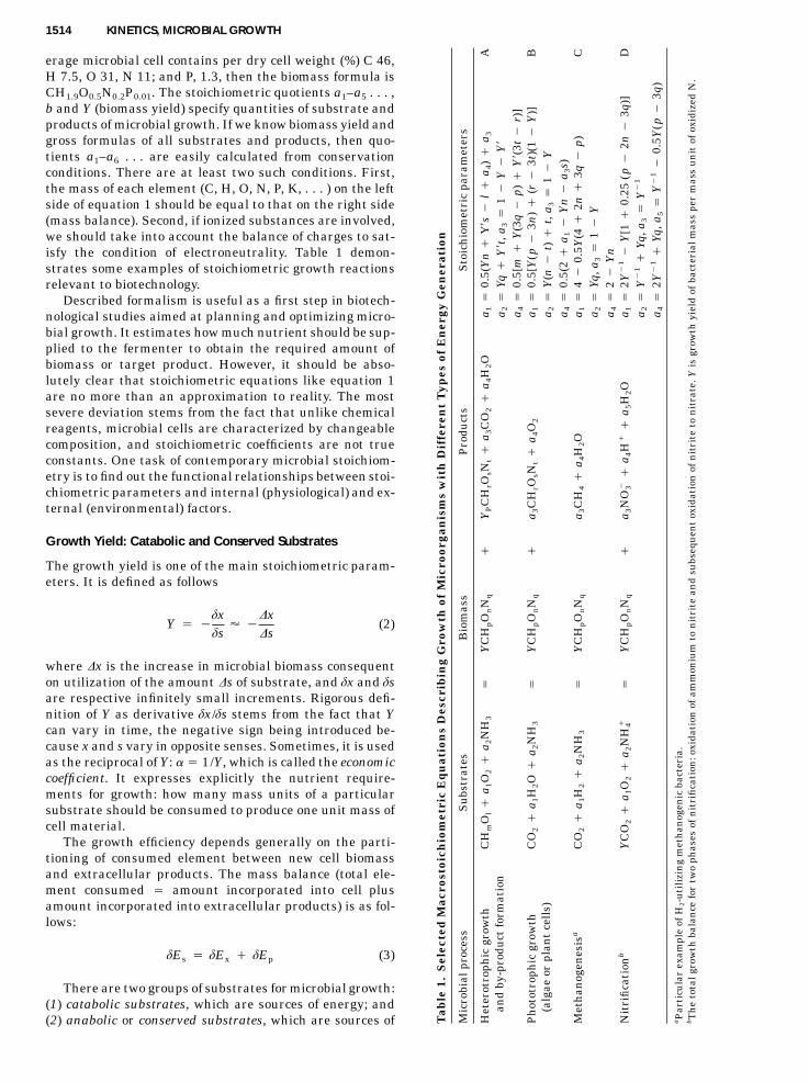
erage microbial cell contains per dry cell weight (%) C 46,H 7.5, O 31, N 11; and P, 1.3, then the biomass formula isCH1.9O0.5N0.2P0.01. The stoichiometric quotients a1–a5 . . . ,b and Y (biomass yield) specify quantities of substrate andproducts of microbial growth. If we know biomass yield andgross formulas of all substrates and products, then quo-tients a1–a6 . . . are easily calculated from conservationconditions. There are at least two such conditions. First,the mass of each element (C, H, O, N, P, K, . . . ) on the leftside of equation 1 should be equal to that on the right side(mass balance). Second, if ionized substances are involved,we should take into account the balance of charges to sat-isfy the condition of electroneutrality. Table 1 demon-strates some examples of stoichiometric growth reactionsrelevant to biotechnology.
Described formalism is useful as a first step in biotech-nological studies aimed at planning and optimizing micro-bial growth. It estimates how much nutrient should be sup-plied to the fermenter to obtain the required amount ofbiomass or target product. However, it should be abso-lutely clear that stoichiometric equations like equation 1are no more than an approximation to reality. The mostsevere deviation stems from the fact that unlike chemicalreagents, microbial cells are characterized by changeablecomposition, and stoichiometric coefficients are not trueconstants. One task of contemporary microbial stoichiom-etry is to find out the functional relationships between stoi-chiometric parameters and internal (physiological) and ex-ternal (environmental) factors.
Growth Yield: Catabolic and Conserved Substrates
The growth yield is one of the main stoichiometric param-eters. It is defined as follows
dx DxY � � � � (2)
ds Ds
where Dx is the increase in microbial biomass consequenton utilization of the amount Ds of substrate, and dx and dsare respective infinitely small increments. Rigorous defi-nition of Y as derivative dx/ds stems from the fact that Ycan vary in time, the negative sign being introduced be-cause x and s vary in opposite senses. Sometimes, it is usedas the reciprocal of Y: � � 1/Y, which is called the economiccoefficient. It expresses explicitly the nutrient require-ments for growth: how many mass units of a particularsubstrate should be consumed to produce one unit mass ofcell material.
The growth efficiency depends generally on the parti-tioning of consumed element between new cell biomassand extracellular products. The mass balance (total ele-ment consumed � amount incorporated into cell plusamount incorporated into extracellular products) is as fol-lows:
dE � dE � dE (3)s x p
There are two groups of substrates for microbial growth:(1) catabolic substrates, which are sources of energy; and(2) anabolic or conserved substrates, which are sources of

KINETICS, MICROBIAL GROWTH 1515
biogenic elements forming cellular material. Catabolicsubstrates include H2 for lithotrophic hydrogen bacteria,
and for nitrifying bacteria, S0 for sulfur-� �NH NO4 2
oxidizing bacteria, oxidizable or fermentable organic sub-stances for heterotrophic bacteria and fungi, and so on.Their consumption is accompanied by oxidation and dis-sipation of chemical substances into extracellular wasteproducts that are no longer reusable as an energy source*(H2O, , CO2, etc.) The anabolic substrates after� 2�NO , SO3 4
uptake are incorporated into de novo synthesized cell com-ponents, being conserved in biomass (that is why they arecalled conserved). Contrary to catabolic substrates, theycan be reused (e.g., after cell lysis to be taken up by sur-vived cells). The conserved substrates include nearly allthe noncarbon sources of biogenic elements (N, P, K, Mg,Fe, and trace elements), CO2 for autotrophs, and the in-dispensable amino acids and growth factors. Most cata-bolic substrates are used also as a source of biogenic ele-ments. We can assess both these components separately interms of respective yields, YE (biomass yield per mass unitof oxidized substrate) and YA (biomass yield per massunit of assimilated substrate), from the experimentallymeasured yield Y. For C substrate, equation 4 can be spec-ified as follows (total carbon consumed equals C incorpo-rated into cell plus C oxidized to CO2 to provide energyplus C incorporated into by-products):
dC � dC � dC � dC (4)s x CO P2
Let us neglect the last term dCP (by assuming that extra-cellular by-products can be reused and functionally areequivalent to C substrate) and divide the substrate balanceby dCx, which is the amount of biomass C produced, then:
1 1� 1 � (5)
Y YE
where Y � g biomass C g�1 substrate C and YE � g bio-mass C g�1 CO2-C
1 r 12x� � (6)
Y r Y rs E s
where Y � g CDW g�1 substrate, YE � g CDW mmol�1
CO2, and rx and rs are fractions of carbon in biomass andsubstrate, respectively. For example, if total measurableyield Y is 0.6 g biomass C g�1 glucose C, it means thatfrom each g of consumed C, 0.6 g is incorporated into bio-mass (assimilated), and 0.4 g is dissimilated (oxidized toCO2), then YE � 0.6/0.4 � 1.5. To calculate oxygen demandfor aerobic growth (or biomass yield on O2) we have a bal-ance (oxygen required to produce 1 g CDW equals oxygenrequired to burn substrate consumed to produce 1 g CDWminus oxygen required to burn 1 g CDW):
*Fermentation products such as acetate, ethanol, butyrate, andH2 seem to be an exception because they do contain reusable ox-idation potential, but it is not available under anaerobic conditionssupervising fermentation.
1/Y � A/Y � B (7)O2
where A and B are constants estimated from stoichiometryof their respective combustion reactions (see equation 10later), for example, the value of A is 33.33 mmol O2 g�1
glucose and B is about 42 mmol O2 g�1 CDW. The rela-tionship between biomass yields on O2 and CO2 is derivedfrom comparison of equations 6 and 7:
Y A � BYCO2 � (8)Y r � r YO s x2
Now we will go back to the general substrate balance(equation 3) and derive an expression for conserved sub-strate. Again, we neglect term dEP (because extracellularproducts are assumed to be reusable) and divide the bal-ance by dx, which is the amount of biomass produced:
1 dEx� � r (9)xY dx
where rx is the intracellular content of element incorpo-rated into biomass from consumed substrate. Sometimesrx is called the cell quota. The values 1/Y and rx are notidentical although they have the same dimension (e.g., mil-ligram N per gram biomass) and very close numeric value.The reciprocal 1/Y is characterizing the process (the expen-diture of conserved substrate to synthesize biomass unit),whereas rx is an index of cell composition (the content ofintracellular N per biomass unit). Formally, 1/Y is equalto the rx value of an infinitely small increment of cell bio-mass, and rx is the averaged value for entire cell. Noticethat although rx is a slow and 1/Y is a rapid variable, theirnumerical values are exactly the same for balanced steady-state growth and can differ considerably during transients.
Yield Variation as Dependent on the Chemical Nature ofOrganic Substrates
In this section, we will discuss why biomass yield varieswhen microorganisms are grown on different C substrates.This problem was best solved within the framework of thetheory of mass and energy balance (TMEB) (3). Evidently,the fraction of C in dry biomass is almost constant. By con-trast, the content of carbon in utilized substrates, rs, andenergetic quality of substrate vary over a broad range (e.g.,compare methane versus oxalic acid). To characterize sub-strate and biomass by a single common measure, TMEBuses an index of degree of carbon reduction, c related to theinternal energy of organic compounds. The heat liberatedby biological or chemical oxidation is proportional to oxy-gen uptake or equally to the number of electrons gained byoxygen from oxidized substrates, according to Payne’s termavailable electrons (ae) (4). The heat production from anoxidation reaction averages at 27 kcal per ae equivalent.A carbon reduction degree, c is defined as the number ofae per one carbon atom. Its numeric value can be deter-mined from the stoichiometry of the oxidation reaction:
CH O N � bO � CO � 0.5(p � 3q)H O � qNHp n q 2 2 2 3
(10)
1516 KINETICS, MICROBIAL GROWTH
c � 4b � 4 � p � 2n � 3q (11)
The ae balance for equation 1 can be written as
c � b(�4) � Yc � Y c (12)s x P p
where cs, cx, and cp are the carbon reduction degree of, re-spectively, substrate, biomass, and extracellular product.Dividing both sides of equation 1 by cs we obtain the re-lationship delineating the ae distribution between oxygen(ae used for respiration), biomass, and the intracellularproduct:
4b Yc Y cx P p� � � 1 (13)
c c cs s s
The second term in this equation is the fraction of ae trans-ferred to biomass from utilized substrate, termed the en-ergetic growth yield.
g � Y c /c (14)C x s
The third term designates that fraction of total substrateinternal energy that is transferred to the product. It iscalled the energetic product yield
f � Y c /c (15)P p s
Energetic yield g is related to other stoichiometric param-eters as follows:
g � Yr c /(r c )x x s s
g � Y c /cC x s
where Y is g CDW/g substrate and YC is g CDW-C/g sub-strate C.
The advantage of using g is that it varies within a muchsmaller range than other yield expressions. At one and thesame efficiency of energy utilization (g), the conventionalbiomass C yield YC is proportional to substrate reductiondegree cs and, for example, it is four times higher on glu-cose (cs � 4) than on oxalate (cs � 1), 0.48 and 0.12 g Cg�1 C, respectively (assuming g � 0.5 and cx � 4.2). Theenergetic growth yield g is more or less constant (0.5 to 0.7)for substrates with cs � 4.2 (4.2 corresponds to averagereduction degree of microbial biomass), and it declines athigher cs.
The attractiveness of macrostoichiometry and TMEB isthat all growth coefficients are interrelated and could bemeasured from any available components of the culturemass balance. For example, if you cannot record microbialgrowth by conventional routine as dry weight biomass (be-cause of presence of solids in broth liquid), you may stillcalculate it from N or O2 uptake, CO2 evolution, pH titra-tion rate, and so on.
Variations in Yield from Energy Source, MaintenanceRequirements
To multiply and grow cells requires energy, but the oppo-site is not true: cells do not require growth to spend energy.
Sometimes catabolic machinery is entirely wasteful (res-piration without cell growth) and always at least some mi-nor part of energy consumption is diverted from growth.To account for this phenomenon, it was postulated thatmicrobes and cells require energy not only for growth butalso for other maintenance purposes. Certain specific main-tenance functions recognized now are turnover of cell ma-terial, osmotic work to maintain concentration gradientsbetween the cell and its exterior, and cell motility.
According to conventional definition of maintenance (5),the balance of energy source is total energy source con-sumed equals consumption for cell growth plus consump-tion for maintenance:
dS � dS � dS (16)E G M
Let us divide it by dx, the amount of biomass produced,then
1 dS dS 1 mG M� � � � (17)maxY dx dx Y l
Here, Ymax � dx/dSG is true growth yield, that is, yieldunder imaginary conditions of maintenance being zero.The maintenance coefficient, m, is introduced as the spe-cific (i.e., expressed per unit of biomass) rate of energy con-sumption for maintenance functions: m � (1/x)(dSM/dt).The ratio m/l on the right side of equation 17 was derivedas follows: m/l � [(1/x)(dSM/dt)]/[(1/x)(dx/dt)] � dSM/dx.
If we divide equation 16 by xdt (note that the secondterm is dSG/(xdt) � [dx/(xdt)]/[dx/dSG] � l/Ymax), then wehave:
maxq � l/Y � m (18)
where q is specific rate of energy source consumption, q �(1/x)(dSE/dt).
It should be noticed that Ymax is a parameter, but notthe yield of a real culture that always has some nonzeromaintenance requirements. It is a very common mistakein the application of the maintenance concept to a partic-ular organism: to take the real measured Y value and pickup from literature some average m coefficient. The correctway would be either to borrow concurrently two parame-ters Ymax and m or to treat actually observed Y as a vari-able that is altered along with specific growth rate l ac-cording to equation 17:
maxlYY � (19)maxl � mY
There is another way to formulate maintenance re-quirements by stating that the net growth of cells l is thedifference between true growth (ltrue) and endogenous de-cay of cellular components (specific rate, a):
l � l � atrue
l � l � atrue
Then, for the rate of energy source uptake, we have

KINETICS, MICROBIAL GROWTH 1517
Y, g
biom
ass
g–1
glu
cose
End
ogen
ous
resp
irat
ion,
mm
ol O
2 h
–1 g
–1
Specific growth rate, (h–1)0
00.1 0.2
00
0.2
0.4
0.025 0.05
0.3 0.40
0.1
0.2
0.3 3
4
2
1
0.4
µ
Figure 1. Variation of growth yield (circles) and endogenous res-piration (squares) as dependent on specific growth rate in che-mostat (open symbols) and continuous dialysis culture (closedsymbols). Solid curves were calculated from the synthetic che-mostat model (2). The dotted curve was derived from the Pirt-Herbert model (equations 17 to 20), which predicts quite well in-tensive growth but fails in the region of extremely low growthrates (see inset).
lx l x (l � a)xtrue� �max maxY Y Y
or
1 1 a� � (20)max maxY Y lY
Comparing equations 17 and 20, we see that a � mYmax.
Experimental Determination of m
To practically determine the maintenance coefficient, themicroorganisms are grown in chemostat culture limited byenergy sources at several dilution rates D (numerically Dis equal to specific growth l if steady state is achieved). Ateach D, we have to measure steady-state biomass x and atleast one of the following quantities (1) residual substrate,s to calculate Y � x/(s0 � s); and (2) the rate of respectiveenergy-yielding process, such as respiration rate, vresp,from O2 uptake or CO2 production rates to calculate spe-cific metabolic activity, q � vresp/x. These data are fitted toequations 17 or 18, m and Ymax being found as nonlinearregression parameters. An example is presented in Figure1. Most available experimental data do obey this relation-ship. However, considerable deviation occurs at very lowgrowth rates usually attained in chemostat with biomassretention or in dialysis culture. The experimental Y valuesfor slowly growing cells are higher than predicted by equa-tions 17 and 18 (see inset on Figure 1). The explanation isvery simple: the maintenance coefficient varies in responseto nutritional status and could not be taken as an absoluteconstant; under substrate deficiency, the cells adjust theirmaintenance requirements to lower values by reducingturnover rate, osmotic work, and motility (2).
The described experimental technique is indirect be-cause it is based on measurements of l-dependent Y vari-ation rather than m itself, and there are some assumptionsneeded to be confirmed (e.g., that m is constant and thatmaintenance requirements are the only reason of Y vari-ation). However, some components of maintenance re-quirements are available for direct estimation. In partic-ular, we can assess the total turnover rate of cellularmaterial a which is one of the main components of main-tenance requirements (equation 20). The principal cell con-stituents that are turned over are proteins, nucleic acids,and cell wall polymers. The turnover rate is very close toendogenous respiration, which is the oxidation of thosecompounds produced from the turnover (breakdown) of cel-lular macrocomponents. Accurate measurements of endog-enous respiration need to be made under normal growingconditions. It is known that the simple removal of cellsfrom nutrient broth by filtration with subsequent washingand incubation in buffer renders strong stress and mayalter the normal turnover rate (6). To avoid artifacts, wecan use a label-substitution technique (Fig. 2). The che-mostat culture is fed alternately from two bottles contain-ing unlabeled and labeled 14C(U) substrate respectively.The 14CO2 evolution rate is recorded after switching to un-labeled substrate, when the main source of 14CO2 are cellcomponents. The calculated a value was found to be ratherhigh, accounting for the major part of total maintenancedetermined by the indirect method (2). The endogenousrespiration declined at the low growth rate (Fig. 1), indi-cating that under starving conditions, self-adjustment ofthe maintenance requirement occurs mainly as a reductionin the turnover rate of macromolecules.
Maintenance Requirements and Wasteful Catabolism
The described concept of maintenance requirements wasthe subject of severe criticism (8). One of the strongest ar-guments against it was an apparent increase in Ymax ob-served in chemostat cultures limited by P, N, and otherconserved substrates under conditions of energy excess. Topreserve the constancy of the true yield, Pirt (9) had tomodify equation 18 in the following way:
maxq � l/Y � m � m�(1 � l/l ) (21)m
where m�(1 � l/lm) is the second l-dependent componentof maintenance energy that operates under excess of en-ergy substrate.
However, it is better to differentiate maintenance re-quirements sensu stricto as those more or less a minor com-ponent of the cell energy budget that is observed underenergy-limitation and wasteful use of catabolic substrateunder energy excess. In physiological terms, these twogroups of nonproductive catabolic reactions are completelydifferent. The first reactions are mainly responsible forcompensation of turned-over macromolecules and there-fore belong to the category of regular primary catabolism.The catabolic reactions of the second group include excre-tion into environment of partly oxidized substances (over-flow metabolism), uncoupling of respiration from ATP gen-eration by metabolic inhibitors, functioning of futile cycles,

1518 KINETICS, MICROBIAL GROWTH
CO
2, m
g C
L–1
Time (h)0 0.5 1 1.5 2 2.5
0
5
10
Total CO214C
15
12C
CO2
14C
Figure 2. Label substitution technique for determination of turn-over rate of cell macromolecular constituents. Top, experimentalsetup including two medium reservoirs containing 14C- and 12C-glucose pumped into a cultivation vessel through a two-way valve.Bottom, example of 14CO2 evolution dynamics before and after (ar-row) switching of medium feed from 14C to 12C-glucose, glucose-limited culture of Pseudomonas fluorescens 1472, D � 0.08h�1 (7).
YN, 1
09 c
ell m
g–1
N
σ N, m
g N
10
–9 c
ell
Specific growth rate, h–10 0.05 0.1 0.15 0.2 0.25
0.8 0.5
0.8
1.1
1.4
1.2σN
YN1.6
2
Figure 3. Relationship between stoichiometric parameters Y ands and specific growth rates of Chlorella vulgaris grown in che-mostat culture limited by nitrogen source (10). The curves arecalculated using equations 23 and 24.
or substrate oxidation through alternative oxidases with-out ATP generation. These and related phenomena takeplace in chemostat culture limited by conserved substrates(opposite to limitation by energy source) as well as duringlag phase of batch culture started from starving inoculum.We will discuss the mathematical formulation of these phe-nomena in the section devoted to growth kinetics.
Variation in Biomass Yield from Conserved Substrates
Yield on conserved substrates varies mainly as a result ofalterations in biomass chemical composition expressed byparameter rs, the intracellular content of deficient elementor cell quota (see equation 9). For most of known cases, thecontent rs increases parallel to growth acceleration (Fig.3). As yield and cell quota are inversely related to eachother (equation 9), then Y values decrease with growthrate. The physiological mechanisms of this variation areas follows. The intensive growth requires higher internal
concentration of some conserved limiting substrates thatpreserve their chemical identity after uptake (K�, Mg2�,vitamins). Other conserved substrates (sources of P, N, S,etc.) are incorporated into macromolecular cell constitu-ents (mainly nucleic acids and proteins) whose intracellu-lar content also should be kept high at high growth rate.Both types of changes in cellular composition are mani-fested as r increase, and both of them require additionalmaintenance energy (to maintain concentration gradientor compensate turnover of macromolecules). The observedl-dependent variation in r is therefore a compromise be-tween biosynthetic requirements and energy conservationthat is attained because of optimal metabolic control of cellperformance. However, it would be erroneous to considerl as truly independent variable setting up chemical com-position of cells. In fact, both l and r are functions of onecommon independent variable, the limiting substrate con-centration in the medium, s. For steady-state chemostatculture we have:
q 1 Qsl � �
r r K � ss
(r � r )sm 0r � r � (22)0 K � sr
where l is specific growth rate, q is specific substrate up-take rates; r0 and rm are, respectively, lower and upperlimits of r variation; low limit r r r0 is attained when s r
0 and upper limits r r rm-when s r �. By excluding s fromboth these equations we arrive at following relationshipbetween r and l:
r (r � r )m 0l � lm
r[k(r � r ) � r � r ]m 0 0
Ksk � (23)
Kr
Under realistic assumption k � 1 (Ks � Kr) we have
KINETICS, MICROBIAL GROWTH 1519
Freq
uenc
y
YATP, g CDW mol–1
5 10 15
Unreliable data
Reliable data
20–0.1
0
0.1
0.2
0.3
0.4
0.5
0.6
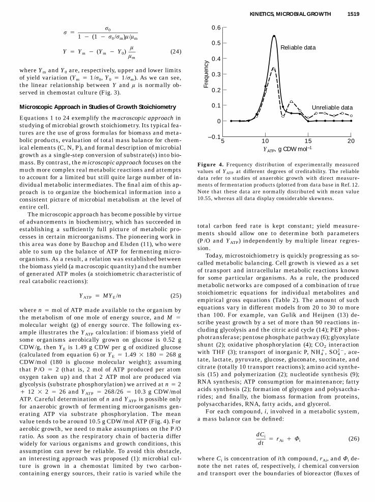
Figure 4. Frequency distribution of experimentally measuredvalues of YATP at different degrees of creditability. The reliabledata refer to studies of anaerobic growth with direct measure-ments of fermentation products (plotted from data base in Ref. 12.Note that these data are normally distributed with mean value10.55, whereas all data display considerable skewness.
r0r �
1 � (1 � r /r )l/l0 m m
lY � Y � (Y � Y ) (24)m m 0
lm
where Ym and Y0 are, respectively, upper and lower limitsof yield variation (Ym � 1/r0, Y0 � 1/rm). As we can see,the linear relationship between Y and l is normally ob-served in chemostat culture (Fig. 3).
Microscopic Approach in Studies of Growth Stoichiometry
Equations 1 to 24 exemplify the macroscopic approach instudying of microbial growth stoichiometry. Its typical fea-tures are the use of gross formulas for biomass and meta-bolic products, evaluation of total mass balance for chem-ical elements (C, N, P), and formal description of microbialgrowth as a single-step conversion of substrate(s) into bio-mass. By contrast, the microscopic approach focuses on themuch more complex real metabolic reactions and attemptsto account for a limited but still quite large number of in-dividual metabolic intermediates. The final aim of this ap-proach is to organize the biochemical information into aconsistent picture of microbial metabolism at the level ofentire cell.
The microscopic approach has become possible by virtueof advancements in biochemistry, which has succeeded inestablishing a sufficiently full picture of metabolic pro-cesses in certain microorganisms. The pioneering work inthis area was done by Bauchop and Elsden (11), who wereable to sum up the balance of ATP for fermenting micro-organisms. As a result, a relation was established betweenthe biomass yield (a macroscopic quantity) and the numberof generated ATP moles (a stoichiometric characteristic ofreal catabolic reactions):
Y � MY /n (25)ATP E
where n � mol of ATP made available to the organism bythe metabolism of one mole of energy source, and M �molecular weight (g) of energy source. The following ex-ample illustrates the YATP calculation: if biomass yield ofsome organisms aerobically grown on glucose is 0.52 gCDW/g, then YE is 1.49 g CDW per g of oxidized glucose(calculated from equation 6) or YE � 1.49 � 180 � 268 gCDW/mol (180 is glucose molecular weight); assumingthat P/O � 2 (that is, 2 mol of ATP produced per atomoxygen taken up) and that 2 ATP mol are produced viaglycolysis (substrate phosphorylation) we arrived at n � 2� 12 � 2 � 26 and YATP � 268/26 � 10.3 g CDW/molATP. Careful determination of n and YATP is possible onlyfor anaerobic growth of fermenting microorganisms gen-erating ATP via substrate phosphorylation. The meanvalue tends to be around 10.5 g CDW/mol ATP (Fig. 4). Foraerobic growth, we need to make assumptions on the P/Oratio. As soon as the respiratory chain of bacteria differwidely for various organisms and growth conditions, thisassumption can never be reliable. To avoid this obstacle,an interesting approach was proposed (1): microbial cul-ture is grown in a chemostat limited by two carbon-containing energy sources, their ratio is varied while the
total carbon feed rate is kept constant; yield measure-ments should allow one to determine both parameters(P/O and YATP) independently by multiple linear regres-sion.
Today, microstoichiometry is quickly progressing as so-called metabolic balancing. Cell growth is viewed as a setof transport and intracellular metabolic reactions knownfor some particular organisms. As a rule, the producedmetabolic networks are composed of a combination of truestoichiometric equations for individual metabolites andempirical gross equations (Table 2). The amount of suchequations vary in different models from 20 to 30 to morethan 100. For example, van Gulik and Heijnen (13) de-scribe yeast growth by a set of more than 90 reactions in-cluding glycolysis and the citric acid cycle (14); PEP phos-photransferase; pentose phosphate pathway (6); glyoxylateshunt (2); oxidative phosphorylation (4); CO2 interactionwith THF (3); transport of inorganic P, , ace-� 2�NH , SO4 4
tate, lactate, pyruvate, glucose, gluconate, succinate, andcitrate (totally 10 transport reactions); amino acid synthe-sis (15) and polymerization (2); nucleotide synthesis (9);RNA synthesis; ATP consumption for maintenance; fattyacids synthesis (2); formation of glycogen and polysaccha-rides; and finally, the biomass formation from proteins,polysaccharides, RNA, fatty acids, and glycerol.
For each compound, i, involved in a metabolic system,a mass balance can be defined:
dCi� r � U (26)Ai idt
where Ci is concentration of ith compound, rAi, and Ui de-note the net rates of, respectively, i chemical conversionand transport over the boundaries of bioreactor (fluxes of

1520 KINETICS, MICROBIAL GROWTH
Table 2. Metabolic Networks
Reaction EquationStoichiometric
EquationEmpirical Gross
Equation
Glycolysis reaction Glucose � ATP r glucose-6-P � ADP � H xGlucose-6-P r fructose-6-P x0.5 Fructose-6-P � 0.5 ATP r glyceraldehyde-3-P � 0.5 ADP � 0.5 H x
Oxidativephosphorylation
NADH � 0.5O2 � d1ADP � d2Pi � (1 � d1) H r (1 � d1)H2O � NAD� d1ATP
x
Biomass formation a1Proteins � a2polysaccharides � a3RNA � a4lipids r biomass x
CO2, O2, nutrients, cells, and products). Most metabolicbalancing equations are applied to steady-state growth(which means that no intracellular accumulation of me-tabolites occurs). In such cases, the differential equationslike equation 26 are reduced to linear algebraic ones. Be-sides, an extensive use of matrix calculus is customarilymade to obtain a concise notation. The problem of experi-mental support of such model is especially important (13).The degree of freedom, df, of the resulting system of linearequations is equal to the total number of unknown rates(both intracellular and exchange reactions) minus the totalnumber of linear equations. To resolve the system, df rateshave to be measured, and then the system is fully deter-mined. If the number of measured rates is greater than df,then the system is overdetermined, and the redundancy ofthe data can be used for statistical analysis and error min-imization. However, it is much more typical to have an un-derdetermined system when the sum of measured rates isless than df. In this case, the number of possible solutionsis infinite unless additional constraints are applied (e.g.,maximization of biomass yield, minimization of energy ex-penditure) to find the one and only one solution by the lin-ear optimization technique.
In most studies, flux estimates are obtained using mea-surements of substrate consumption and product forma-tion. This approach has proved to be efficient in some par-ticular biotechnological cases, such as when only specificpathways need to be considered (16) or if the contributionof flux for cellular growth is weak, as with mammalian orhybridoma cells (17). The more complex microbial systemsare turned out to be seriously underdetermined. In suchcases, the application of metabolic balancing requires theuse of one or another maneuvers: (1) to lump together sev-eral sets of reactions (18); (2) to utilize data from in vitroenzyme assays; (3) to make assumptions on numeric val-ues of some stoichiometric growth parameters, such asYATP, P/O, and H�/e ratios, which are the subject of con-troversial debates (13).
However, the best solution would be to get direct exper-imental data on in vivo flux and resolve the system. Iso-topic tracers are one of the best candidates for such a pur-pose. We will illustrate this point by describing a recentlypublished work (19). This novel approach is based on theanalytical power of 1H-detected 13C nuclear magnetic res-onance. Corynebacterium glutamicum was grown in che-mostat culture continuously fed with [1-13C]-glucose; whensteady state was established, the cells were harvested andhydrolyzed and the amino acids were separated by ion-exchange chromatography and analyzed by NMR spectros-
copy. NMR provides data on 13C enrichment at each spec-ified carbon position of amino acid. Because metabolicpathways for amino acid synthesis are exactly defined,then the entire central metabolism can be assessed for invivo fluxes, including determination of the forward andback rates of bidirectional reactions. In C. glutamicum, theflux through the pentose phosphate pathway turned out tobe 66.4% (relative to glucose input flux 1.49 mmol g�1
CDW h�1); the entry into tricarboxylic acid cycle, 62.2%,and the contribution of the succinylase pathway to lysinesynthesis, 13.7%. The total net flux of the anaplerotic re-actions (carboxylation of PEP/pyruvate into oxaloacetate/malate) was quantitated as 38%, the true forward flux ofC3 r C4 being 68.6% (1.8 times of 38%) and a back flux ofC4 r C3 being 30.6% (0.8 times of 38%) (19). The metabolicbalancing proved to be very promising and useful to iden-tify metabolic constraints for intensive synthesis (overpro-duction) of products such as amino acids. On the otherhand, this approach still is restricted to steady-state andbalanced growth and is not able to cope with complex dy-namic behavior of microorganisms (transient growth,changes in biomass composition).
BASIC PRINCIPLES OF GROWTH KINETICS
Kinetics of Chemical and Enzyme Reactions
We need to introduce some basic principles of kinetic anal-ysis of chemical and enzymatic reactions. Quantitative de-scription and understanding of microbial growth dynamicsand kinetics are impossible without some elementaryknowledge in underlying scientific disciplines. Enzymaticand chemical reactions play an essential role in biotech-nology, which is one of the most important fields in indus-trial development.
Order and Molecularity of Chemical Reactions. The mo-lecularity of any chemical reaction is defined by the num-ber of molecules that are altered in the reaction (Table 3).The order is a description of the number of concentrationterms multipled together in the rate equation (Table 4).Hence, in a first-order reaction, the rate is proportional toone concentration of reactant; in a second-order reaction,it is proportional to two concentrations or to the square ofone concentration. For a simple single-step reaction, theorder is generally the same as the molecularity. For a com-plex reactions involving a sequence of unimolecular andbimolecular steps, the molecularity is not the same as itsorder. Reactions of molecularity greater than 2 are com-
KINETICS, MICROBIAL GROWTH 1521
Table 3. Molecularity of Chemical Reaction
Molecularity of reaction Reactants Product
Unimolecular or monomolecular S r PBimolecular S � S r Por S1 � S2 r PTrimolecular or termolecular S � S � S r Por S1 � S1 � S2 r Por S1 � S2 � S3 r P
Table 4. Kinetic Order of Chemical Reactions
Reactionorder
Differentialequation
Dimension ofrate constant
Dynamics ofresidual reactant
Dynamics ofproduct accumulation
Reactionhalf-timea
Zerods
� �kdt
(conc.)(time)�1 s(t) � s0 � kt p(t) � p0 � kts0t �0.5 2k
First � �ksdsdt
(time)�1 s(t) � s0 exp(�kt) p(t) � s0[1 � exp(�kt)]ln2
t �0.5 k
Secondds 2� �ksdt
(conc.)�1(time)�1 s0s(t) �1 � ks t0
2s kt0p(t) �2(1 � s kt)0
b1t �0.5 ks0
Seconddp
� �ks s1 2dt(conc.)�1(time)�1 s1(t) � s01 � p(t)
s2(t) � s02 � p(t)s s (1 � exp[(s � s )kt])01 02 02 01p(t) �s � s exp[(s � s )kt]01 02 02 01
� 1/ks01t�0.5
t� � 1/ks0.5 02
Pseudo-firsts01 � s02
dp� �ks s1 2dt
(conc.)�1(time)�1 s2(t) � s02 exp(�ks01t)s1(t) � s01
p � s02[1 � exp(�ks01t)]
Note: t � time; s � reactant concentration; p � product concentration; s0 � reactant concentration at t � 0.aThe half-time of the reaction is the time required for half-completion.bThe half-time is defined for the reagent that has lower initial concentration and is depleted first.
mon, but reactions of order greater than 2 are very rare.For instance, a trimolecular reaction, such as A � B � Cr P, as a rule proceeds through two elementary steps, A� B r X and X � C r P, each of which are of the secondor first order. Very often, bimolecular reactions between S1
and S2 occur under the condition that their respective con-centrations s2 � s1 (e.g., if the second reactant S2 is sol-vent), then we have a pseudo first-order reaction. Some re-actions are observed to be of the zero order, that is, the rateappears to be constant, independent of the concentrationof reactant. This is a characteristic feature of catalyzedreactions and occurs if reactant is present in such largeexcess that the full potential of catalyst is realized.
Dimensions of Rate Constants. Knowledge of dimensionsis very useful to check the correctness of derived kineticequations: the left- and right-hand sides of an equationmust always have the same dimensions. This general ruleis applicable to all mathematical models (not only in chem-ical kinetics). It is incorrect to add or subtract terms ofdifferent dimensions, although you may multiply or dividethem. For example, if expression “ . . . (1 � s)” occurs inan equation, where s has dimension (concentration), theneither equation is incorrect, or the 1 is a concentration thathappens to have a numerical value of 1 unit. The operationrising to power is allowed for only simple dimensionlessnumbers, for example, expression e2.5t, where t is time, iscorrect only if 2.5 has dimension (time)�1. The comparisonof velocities of two reactions does make any sense only forkinetic terms of the same dimension. If the kinetic order
of inspected reactions is different, then we have to equalizethe respective rate of expressions; for example, the second-order rate constant k (time)�1 (concentration)�1 should bemultiplied by instant concentration of reactant s to be com-pared with the first-order rate constant having dimension(time)�1. The dimensions of the zero-, first-, and second-order rate constants are shown in Table 4.
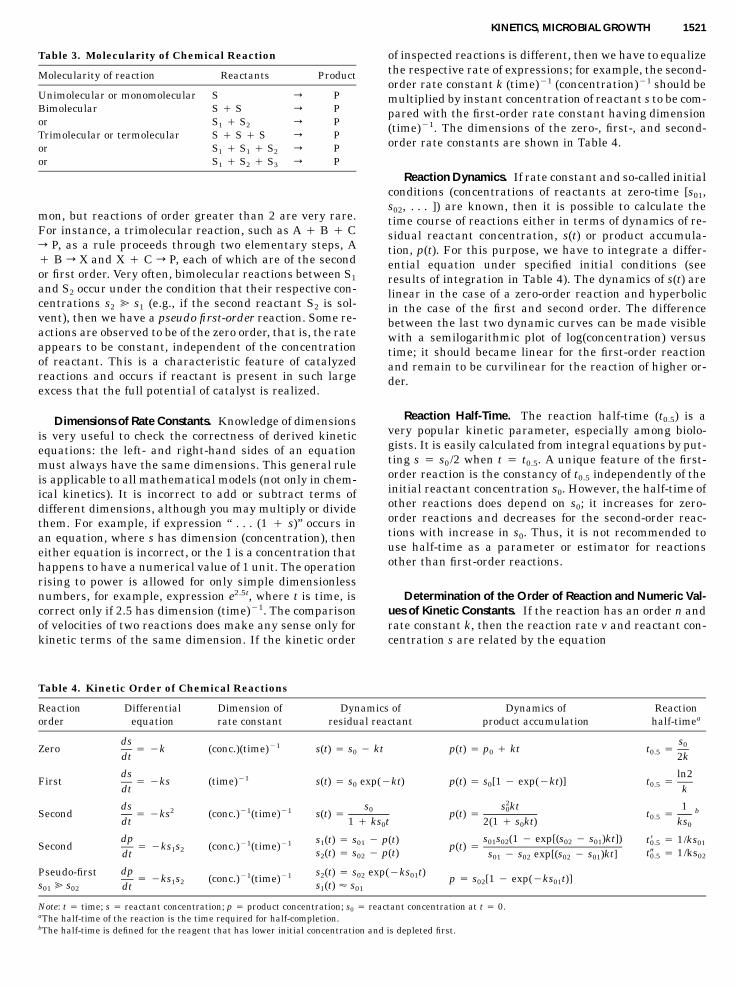
Reaction Dynamics. If rate constant and so-called initialconditions (concentrations of reactants at zero-time [s01,s02, . . . ]) are known, then it is possible to calculate thetime course of reactions either in terms of dynamics of re-sidual reactant concentration, s(t) or product accumula-tion, p(t). For this purpose, we have to integrate a differ-ential equation under specified initial conditions (seeresults of integration in Table 4). The dynamics of s(t) arelinear in the case of a zero-order reaction and hyperbolicin the case of the first and second order. The differencebetween the last two dynamic curves can be made visiblewith a semilogarithmic plot of log(concentration) versustime; it should became linear for the first-order reactionand remain to be curvilinear for the reaction of higher or-der.
Reaction Half-Time. The reaction half-time (t0.5) is avery popular kinetic parameter, especially among biolo-gists. It is easily calculated from integral equations by put-ting s � s0/2 when t � t0.5. A unique feature of the first-order reaction is the constancy of t0.5 independently of theinitial reactant concentration s0. However, the half-time ofother reactions does depend on s0; it increases for zero-order reactions and decreases for the second-order reac-tions with increase in s0. Thus, it is not recommended touse half-time as a parameter or estimator for reactionsother than first-order reactions.
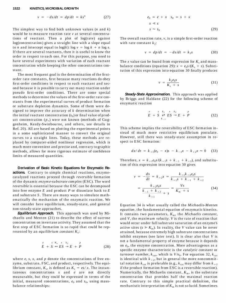
Determination of the Order of Reaction and Numeric Val-ues of Kinetic Constants. If the reaction has an order n andrate constant k, then the reaction rate v and reactant con-centration s are related by the equation
1522 KINETICS, MICROBIAL GROWTH
nv � �ds/dt � dp/dt � ks (27)
The simplest way to find both unknown values (n and k)would be to measure reaction rate v at several concentra-tions of reactant. Then a plot of log(rate) againstlog(concentration) gives a straight line with a slope equalto n and intercept equal to log(k): log v � log k � n log s.If there are several reactants, then it is useful to know theorder in respect to each one. For this purpose, you need tohave several experiments with variation of each reactantconcentration while keeping the other concentrations con-stant.
The most frequent goal is the determination of the first-order rate constants, first because many reactions do obeyfirst-order conditions in respect to each reactant and sec-ond because it is possible to carry out many reaction underpseudo first-order conditions. There are some specialmethods to determine the values of the first-order rate con-stants from the experimental curves of product formationor substrate depletion dynamics. Some of them were de-signed to improve the accuracy of k determination whenthe initial reactant concentration (s0) or final value of prod-uct concentration (p�) were not known (methods of Gug-genheim, Kezdy-Swinbourne, and others, see details inRef. 20). All are based on plotting the experimental pointsin a some sophisticated manner to convert the originalcurves to a straight lines. Today, these methods are re-placed by computer-aided nonlinear regression, which ismuch more convenient and precise and, contrary to graphicmethods, allows for more rigorous estimate of confidencelimits of measured quantities.
Derivation of Basic Kinetic Equations for Enzymatic Re-actions. Contrary to simple chemical reactions, enzyme-catalyzed reactions proceed through reversible formationof the dynamic enzyme-substrate complex (ESC). The wordreversible is essential because the ESC can be decomposedinto free enzyme E and product P or dissociate back to Eand substrate S. There are many ways to simulate math-ematically the mechanism of the enzymatic reaction. Wewill consider here equilibrium, steady-state, and generalnon-steady-state approaches.
Equilibrium Approach. This approach was used by Mi-chaelis and Menten (21) to describe the effect of sucroseconcentration on invertase activity. They assumed that thefirst step of ESC formation is so rapid that could be rep-resented by an equilibrium constant Ks:
e s K x k ps 2
E � S } ES r E � P (28)
where e, s, x, and p denote the concentrations of free en-zyme, substrate, FSC, and product, respectively. The equi-librium constant, Ks, is defined as Ks � es/x. The instan-taneous concentrations s and e are not directlymeasurable, but they could be expressed in terms of theinitial, measured concentrations, e0 and s0, using mass-balance relationships:
e � e � x s � s � x0 0
x � s
s � s (29)0
The overall reaction rate, v, is a simple first-order reactionwith rate constant k2:
v � dp/dt � �ds/dt � k x (30)2
The x value can be found from expression for Ks and mass-balance conditions (equation 29): x � e0s/(Ks � s). Substi-tution of this expression into equation 30 finally produces
k e s2 0v � (31)K � ss
Steady-State Approximation. This approach was appliedby Briggs and Haldane (22) for the following scheme ofenzymatic reaction
e s k x k p1 2
E � S i ES r E � P (32)k�1
This scheme implies the reversibility of ESC formation in-stead of much more restrictive equilibrium postulate.However, still there was steady-state assumption in re-spect to ESC formation:
dx/dt � k (e � x)s � k x � k x � 0 (33)�1 0 �1 �2
Therefore, x � k�1e0s/(k�1s � k�1 � k�2), and substitu-tion of this expression into equation 30 gives
ds k k e s�1 �2 0v � � � k x ��2dt k s � k � k�1 �1 �2
k e s Vs�2 0� � (34)
k � k K � s�1 �2 m� s
k�1
Equation 34 is what usually called the Michaelis-Mentenequation, the fundamental equation of enzymatic kinetics.It contains two parameters, Km, the Michaelis constant,and V, the maximum velocity. V is the rate of reaction thatwould occur under full substrate saturation of an enzyme’sactive sites (s � Km). In reality, the V value can be neverattained, because extremely high substrate concentrationsinhibit enzymes (see later text). It is clear also that V isnot a fundamental property of enzyme because it dependson e0, the enzyme concentration. More advantageous as aspecific enzyme characteristic is the catalytic constant orturnover number, kcat, which is V/e0. For equation 32, kcat
is identical with k�2, but in general the more noncommit-tal notation kcat is preferable (e.g., kcat may differ from k�2
if the product formation from ESC is a reversible reaction).Numerically, the Michaelis constant, Km, is the substrateconcentration that provides half the maximal reactionrate. Contrary to this simple practical definition, themechanistic interpretation of Km is not so lucid. Sometimes

KINETICS, MICROBIAL GROWTH 1523
Inst
ant
reac
tion
rat
e, n
mol
s–1
Time, s (log scale)0.000001 0.001
Transientphase
Steady-statephase Substrate
depletionphase
1 10000
20
40
60
80
100
Figure 5. Time course of reaction proceeding by the Michaelis-Menten mechanism. Numeric integration of equations 33 and 34:s0 � 10�4M, e0 � 10�8M, k�1 � 106M�1s�1, k�1 � 103 s�1, k�2
� 102 s�1.
Km is interpreted as a substrate binding constant, Ks, as-suming that k�2 � k�1. This is a very dubious assumption.There are very few enzymes for which the individual val-ues of k�2 and k�1 are known. Ironically, the best-studiedexamples (e.g., horseradish peroxidase) present just op-posite case: k�2 � k�1. It is important that many specificmechanisms (not necessarily equations 28 and 32) gener-ate the same steady-state rate equation 34. However, theparticular expression for Km should be different for eachindividual case.
Although undefined in mechanistic terms, the param-eters Km and V are very useful at the first steps of kineticstudies:
1. The use of equation 34 allows the expression of thecomplex effects with simpler terms.
2. Km and V are helpful as predictive parameters to de-sign a valid enzyme assay. One practical recommen-dation is to keep substrate concentration in incuba-tion mixture at the level of 10 Km or higher.
3. Equation 34 permits one to obtain at least rough es-timate of in vivo enzyme activity provided the inter-nal substrate concentrations are known.
General Non-Steady-State Approach. Equation 32 con-tains four variables (s, p, e, and x) constrained by two mass-balance equations (e0 � e � x and s0 � s � p � x). There-fore, it is enough to integrate just two differentialequations (e.g., equations 33 and 34) to characterize thewhole system. A typical example of a numeric solution isshown in Figure 5. We can see that enzyme-catalyzed re-action proceeds through three definite phases well sepa-rated on the time scale. Each phase is now safe to analyzewith simpler mathematical expressions because any as-sumptions could be tested against the full exact solution.
1. The first transient phase occurs before the steady-state concentration of ESC is reached. It occupies less than
10�3 s for most of enzymes. During this phase, the sub-strate concentration remains fairly constant (s � s0), allow-ing for the following analytical solution:
k e s Vs�1 0 0 �At �Atx(t) � [1 � e ], v(t) � [1 � e ]A K � cm
A � k s � k � k (35)�1 0 �1 �2
As compared with equation 34, it contains a relaxationterm [1 � exp(�At)] that is very large when t is small, butdecays to zero as t increases above s � 1/A. Accordingly,the rate of enzymatic reaction is initially zero but increasesrapidly to the steady-state value as the exponential termdecays. Because the relaxation term contains s0, then theexperimentally observed delay depends on substrate con-centration. It allows for direct determination of individualrate constants k�1 and (k�1 � k�2) by techniques such asin stopped-flow apparatus (23).
2. The second steady-state phase is characterized bythe constancy of reaction rate due to the exact balance be-tween the rates of ESC formation and breakdown (dx/dt� 0) while the substrate concentration remains close tothe initial value s0. This phase proceeds for at least severalseconds. As a rule, it is enough to measure the initial ve-locity of enzymatic reactions unaffected by substrate de-pletion or product accumulation. Steady-state kinetics isthe most popular research domain; it is the most accessibleand developed and provides the most kinetic data. How-ever, it fails to determine individual rate constants as fullyas the transient and relaxation approaches do. Steady-state equations were derived earlier (equation 34).
3. The third phase is characterized by considerablechanges in the concentrations of substrate and product.Thus, we can no longer assume that s � s0, and we shouldintegrate equations 32 and 33. However, very good preci-sion provides the quasi-steady-state approximation ds/dt� dx/dt � 0. Then, we arrive at a relatively simple differ-ential equation that is solved analytically:
ds Vs(t)� � (36)
dt K � s(t)m
For initial conditions s � s0, p � 0, t � 0, we have
s0K ln � s � s � Vt (37)m 0s
Equation 37 is called the integrated Michaelis-Mentenequation. It remains to be valid not only for initial ratemeasurements but for any point within the reaction pro-gress curve.
Experimental Determination of Kinetic Parameters of theMichaelis-Menten Equation. Until recently, most enzymekinetic experiments have been analyzed by means of oneof linear plots in Table 5. Linear plots are used to examinean agreement of experimental data with equation 34 aswell as to determine numeric values of parameters V andKm from slopes and intercepts. Today, this graphic ap-
1524 KINETICS, MICROBIAL GROWTH
Table 5. Linear Plots
1 1 K 1m� �
v V V sLineweaver-Burk or double-reciprocal plot
s K sm� �
v V VLangmuir-Hanes plot
vv � V � Km s
Eadie-Hofstee plot
vV � v � Kms
Direct linear plot (20)
proach seems to be too cumbersome as compared withmuch more efficient computer routines. The main objectionis also that any linear transformation introduces some sta-tistical bias (ironically, the highest bias is attributed to themost popular double-reciprocal plot!). In addition, manualline drawing is very arbitrary, so obtained parameterscould not be assessed statistically for confidence limits.However, plotting of original or linearized data is useful asan illustration and the first sketchy estimate of enzymaticparameters. For definitive work, it is advisable to avoid allplots and to use statistical analyses instead.
Reversible Enzymatic Reactions. The majority of bio-chemical reactions are reversible. To account for this fea-ture, the Michaelis-Menten mechanism can be modified asfollows:
k k k�1 �2 �3
E � S i ES i EP i E � P (38)e �x�y s k x k y k e �x�y p0 �2 �2 �3 0
Contrary to the basic scheme in equation 32, there are twointermediates, one of which is the normal ESC and anotheris the enzyme-product complex (EP). The substrate, S, andproduct, P, can interconvert to each other. Application ofthe steady-state approach to this scheme results in the fol-lowing equation:
f s r pV s/K � V p/Km mv � s p1 � s/K � p/Km m
k k e�2 �3 0fV �k � k � k�2 �2 �3
k k � k k � k k�1 �2 �1 �3 �2 �3sK �m k (k � k � k )�1 �2 �2 �3
k k e�1 �2 0rV �k � k � k�1 �2 �2
k k � k k � k k�1 �2 �1 �3 �2 �3pK � (39)m k (k � k � k )�3 �1 �2 �2
where superscripts f and s denotes parameters of forwardreaction, and r and p are indicators of reverse reaction.
When a reaction is at equilibrium, the net velocity mustbe zero and, consequently, if s� and p� are the equilibriumvalues of s and p, it follows from equation 39 that equilib-rium constant K is expressed via kinetic parameters (theHaldane relationship):
f p r sK � p /s � V K /V K (40)� � m m
Equation 39 implies that the rate must decrease as theproduct accumulates, even if the decrease in substrate con-centration is negligible. Thus, reversibility is closely as-sociated with and requires the product inhibition. In manyessentially irreversible reactions (e.g., invertase-catalyzedhydrolysis of sucrose), product inhibition is also signifi-cant. It can be explained by equation 38 with only the sec-ond step being irreversible. In such a case, the accumula-tion of product causes the enzyme to be sequesteredbecause the EP complex and rate equation are as follows(compare with equation 39):
f s fV s/K V smv � � (41)s p s p1 � s/K � pK K (1 � pK ) � sm m m m
Inhibitors and Activators. Compounds that reduce therate of enzyme-catalyzed reactions when they are added tothe reaction mixture are called inhibitors. Just oppositeeffects (increase of reaction rate) are caused by activators.Both of them belong to the category of modifiers. We willconcentrate here on inhibitors as having more practical ap-plication and even more specifically on reversible inhibi-tors, which form various dynamic complexes with en-zymes. The irreversible inhibitors are known as catalyticpoisons (many heavy metals, such as mercury); their bind-ing to enzyme molecules reduces activity to zero, leavingno room for quantitative analysis.
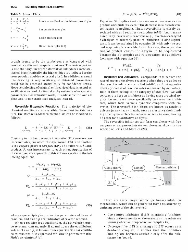
The reversible inhibitors can form complexes with freeenzymes or enzyme-substrate complexes as shown in thescheme of Botts and Morales (20):
Competitive Mixed Uncompetitive
S
P
S
P
E ES
II
EI EIS
There are three major simple (or linear) inhibitionmechanisms, which can be generated from this scheme byomitting some of the six involved:
• Competitive inhibition if EIS is missing (inhibitorbinds to the same site on the enzyme as the substrateforming abortive nonproductive complex EI).
• Uncompetitive if EI is missing and EIS occurs as adead-end complex; it implies that the inhibitor-binding site becomes available only after the sub-strate has bound.

KINETICS, MICROBIAL GROWTH 1525
Table 6. Types of Inhibition
Type of inhibition Vapp Vapp/ appKmappkm
Competitive V (V/Km)/(1 � i/Ki)a Km(1 � i/Ki)Uncompetitive V/(1 � i/K�)i V/Km Km(1 � )i/K�)i
Mixed V/(1 � i/K�)i (V/Km)/(1 � i/Ki) Km(1 � i/Ki)/(1 � i/K�)i
Pure noncompetitive V/(1 � i/K�)i (V/Km)/(1 � i/Ki) Km
• Mixed if EI and EIS both occur but are not intercon-vertible (the complex EIS does not break down toproducts; this situation frequently occurs when theinhibitor is reaction product). The particular case ofmixed inhibition is pure noncompetitive inhibition,which takes place if two inhibitor dissociation con-stants (for EI and EIS) are exactly matched to eachother.
For all types of inhibition, the Michaelis-Menten equa-tion remains valid: under constant inhibitor concentration,i, the v-s relationship is of the same hyperbolic type aspredicted by equation 34, the only difference is that ap-parent values of Km and V are now more or less simplefunctions of i (Table 6).
Some parameters (in boldface in Table 6) are not af-fected by inhibitors, whereas others are changed: compet-itive inhibitors increase Km, pure noncompetitive inhibi-tors reduce V, uncompetitive inhibitors decrease at thesame degree both V and Km, leaving first-order rate con-stant V/Km to be unchanged. In mixed inhibition, there areno unchanged parameters.
One interesting case is so-called substrate inhibition. Itoccurs when two substrates are bound to the same activesite on the enzyme, forming nonproductive triple complexES2:
K kss 2
E � S } ES r E � P@KSS
ES2
then, the enzyme rate (24) is:
Vsv � (42)2K � s � s /Ks ss
where Kss is the dissociation constant for complex ES2.
Cooperativity. Many enzymes respond to changes in me-tabolite concentrations (substrates, modifiers) with muchhigher sensitivity as compared with predictions from theclassic hyperbolic equations 34 to 42. This property is gen-erally known as cooperativity, because it is thought to arisefrom cooperation between the active sites of the polymericenzymes. As a rule, such enzymes consist of several sub-units and display so-called sigmoid or S-shaped depen-dence of rate on substrate concentration. Many cooperativeenzymes (but not all!) have active sites binding substrateand allosteric sites binding effectors. There are homotropicand heterotropic cooperative effects caused by interactions
between, respectively, identical and different ligands (e.g.,substrate and an allosteric effector).
To explain the cooperativity and associated sigmoid ki-netics, a number of models have been suggested. The ear-liest one is the Hill equation, which was originally de-signed to describe the S-shaped curve of oxygen binding tohemoglobin. It was assumed that each protein molecule Ebinds n molecules of ligands S in a single step, an amountof other possible forms (ESn�1, ESn�2, . . . ES) being neg-ligible:
Kh
E � nS } ESn
where Kh is the respective equilibrium constant (Hill andcolleagues described equilibrium in terms of associationconstant, but for the sake of uniformity we will adhere tothe previous formalisms, keeping in mind the dissociationconstant, Kh � [E][S]n/[ESn]). The fractional saturation ofprotein (enzyme or hemoglobin). H is given as
Number of occupied binding sitesH �
Total number of binding sitesn[ES ] [S]n
� � (43)n[E] � [ES ] K � [S]n h
Equation 43 can be rearranged into
nH [S] H� , log � �logK � n log[S] (44)h� �1 � H K 1 � Hh
A plot of log H/(1 � H) against log [S] is known as the Hillplot and should be a straight line of slope n (so). This equa-tion is used to fit the experimental binding and kinetic datadisplaying a sigmoid shape. When plotting kinetic mea-surements, it is assumed that H � v/V, and maximum ve-locity V should be known from independent measurementstaken at saturation substrate concentration. However, theresults of fitting should be interpreted with care. First, theHill equation is empirical and generally provides goodagreement only in the H range 0.1 to 0.9 (the discrepancyat extreme s is probably caused by neglecting of otherforms of ESC apart from ESn). Second, parameter n (Hillcoefficient) could not be interpreted as the number of sub-units in the fully associated protein, rather it is an indexof cooperativity.
Monod et al. (25) proposed a general model explainingcooperativity and allosteric phenomena within a simple setof postulates:
1. Each subunit of enzyme can exist in two differentconformations, designated R (relaxed) and T (tense).

1526 KINETICS, MICROBIAL GROWTH
2. All subunits of a molecule must occupy the same con-formation at any time (e.g., for tetrameric enzymeonly R4 or T4 are permitted, not R3T or R2T2, etc.).
3. The two states are in equilibrium with constant L �[R4]/[T4].
4. The affinity of ligand to subunit depends on the con-formation state: KR � [R][S]/[RS], KT � [T][S]/[TS],c � KR/KT.
The general equilibrium solution of this scheme israther bulky, so we demonstrate one particular case of tet-rameric protein, if c � 0 (i.e., KR � KT, S binds only to theR state), then we have
3(1 � s/K ) s/KR RH � (45)4L � (1 � s/K )R
At high s when s/KR � L, we can neglect the term L in thedenominator, and the entire expression is converted to nomore than the simple hyperbolic Langmuir isotherm. Atlow s, the contribution of L is considerable, so the satura-tion curve rises slowly from the origin displaying theS-shape.
There are other models describing the mechanisms ofcooperativity and allosteric effects (20), for example, thesequential model of Koshland and colleagues and theassociation–dissociation model of Freiden.
Effects of pH. Every enzyme contains a large number ofacidic and basic groups. Some of them are either fully de-protonated (aspartate, glutamate) or fully protonated (ar-ginine, lysine). However several groups with pKa 5 to 9(imidazole group of histidine, sulphydryl group of cysteine)do change their ionization state when pH is varied. As-sume as a first approximation that enzyme is representedas a dibasic acid H2E and only a singly ionized complex,HES�, is able to react to give products:
H E H ES2 2E ES@ K @ Kk k�1 �21 1
� � �S � HE i HES r HE � PE k ES�1@ K @ K2 2
2� 2�E ES
Then the reaction rate is dependent on H� concentration,h, as follows (20):
Vsv �
K � sm
VV � ESh K2
� 1 �� ES �K h1
˜ ˜V V/Km� (46)EK h Km 2
� 1 �� E �K h1
where V and Km are the pH-corrected constants. It is clearthat pH-dependent variation of V reflects the ionization of
ESC, whereas V/Km reflects the ionization of the free en-zyme. The pH effects on Km are more complicated, beingaffected by both. Generally, the dependence of enzyme ac-tivity on pH is described by equation 43 as a bell-shapedcurve with maximum at 1/2(pK1 � pK2).
Effects of Temperature. In chemical kinetics, the depen-dence of reaction rate on temperature is explained by thetransition-state theory developed by Eyring in 1930 to1935. It is based on the use of thermodynamics and prin-ciples of quantum mechanics. The reaction proceedsthrough a continuum of energy states and must surpassthe state of maximum energy, when transient activatedcomplex is formed. Then the dependence of reaction rateconstant k on absolute temperature, T, is expressed as fol-lows:
d lnk DH* � RT� (47)2dT RT
where R is the gas constant and DH* is the enthalpy ofactivated complex formation. The classic Arrhenius equa-tion may be obtained from equation 47 under a simplifiedcondition DH* � RT � DH � Ea (where Ea is activationenergy). Most often, the Arrhenius equation is used in itsintegrated form:
lnk � lnA � E /RTa
or
k � A exp(�E /RT) (48)a
where A is the integration constant, interpreted as the fre-quency of collisions of reacting molecules. Apart frommechanistic derivations, there are a number of empiricalexpressions relating k and Celsius temperature Tc. Themost popular is the exponential formula:
lnk � lnA � �Tc
or
k � A exp(�T ) (49)c
where � is the empirical constant related to the widelyused temperature coefficient Q10 � exp(10 * �).
All presented mathematical expressions predict expo-nential or almost exponential increases of chemical reac-tion rates with temperature. However, enzymatic reac-tions deviate from this relationship at high temperaturebecause of thermal denaturation of enzymes. Assume thatdenaturation is reversible with equilibrium constant KT �[E�]/[E], where E represents active enzyme molecules andE� represents inactive molecules. Then, the combination ofequation 48 with the van’t Hoff relationship for KT (�RTlnKT � DGo � DHo � TDSo) results in
A exp(�E /RT)av � (50)o o1 � exp(DS /R � DH /RT)
where DGo, DSo, and DHo are the standard Gibbs free en-
KINETICS, MICROBIAL GROWTH 1527
Table 7. Major State Variables of Deterministic Models
Variable Notation Dimension (examples)
Concentration of cell biomass x g CDW L�1 of cultural liquidCell numbera N 109 cell mL�1 of cultural liquidSingle-cell massa m g CDW per cellMycelium lengthb L meter L�1 of cultural liquidTips numberb n 106 tips mL�1 of cultural liquidConcentration of limiting substrate s g L�1 of cultural liquidConcentration of product p g L�1 of cultural liquid or g g�1 of CDW
aFor unicellar organisms (bacteria, yeasts).bFor filamentous organisms (fungi, actinomycetes).
ergy, enthalpy, and entropy of denaturation reaction, re-spectively, and v is the observed rate of biological process.This equation produces a curve with single maximum andfits to most of the available experimental data ontemperature-dependent variations of enzymatic activity.
Sometimes denaturation is irreversible, and there areno possibilities for simple mathematical expressions, be-cause temperature effects depends on the exposing time.However, numeric solutions of respective differential equa-tions can still be used.
Simple Models of Microbial and Cell Growth
This section deals with simple unstructured models. Thesemodels mainly ignore any changes in cell quality (biochem-ical composition, spectrum of enzymatic activity, etc.) in-duced by environmental factors.
Main State Variables and Growth Parameters. There aretwo types of growth models, deterministic and stochastic.The former describe clear determined and regular pro-cesses. The latter deal with random or stochastic pro-cesses. The main variables used in deterministic modelsare the same as in chemical kinetics, concentrations of bio-mass, substrates, and products, and stochastic models con-sider instead the probabilities, frequency distributions,variance, and so on. For example, a stochastic model canconsider the probability of a single bacteria cell dividingunder specified environmental conditions. Although anyreal-life biotechnological process has both deterministicand stochastic components, most useful growth models arestrictly deterministic. In this section, we will concentrateon this type of model, and the stochastic counterparts willbe considered only in “Cell Cycle”.
The major state variables of deterministic models de-scribing cell growth are described in Table 7. The concen-tration of biomass and cell number are related to eachother by simple formula:
x � m � N (51)
where conversion factor m1 is the average dry mass of asingle cell. In some studies, it is save to assume m to be aconstant and use both variables x and N as equivalentmeasures of growth. However, the average size and massof single cells vary depending on the nature of studied or-ganisms and environmental conditions (see “Cell Cycle”);
therefore, it is advisable to make a selection. The biomass,x, has obvious advantage in studies aimed at understand-ing or control of mass flows, and cell number, N, is pre-ferred in population studies when, for example, mutationor plasmid transfer is an essential factor controlling theefficiency of the biotechnological process.
The choice of method to determine biomass or cell num-ber depends on many factors (2,5). Today, the preferenceshould be given to those techniques that allow exact andautomated measurements (Table 8). The most advancedanalytical methodology is now available for automatic re-cording of gaseous or volatile substrates, intermediates,and end products, such as methane, CO2, O2, H2, volatilefatty acids, alcohols, and other fermentation products (IR-analyzers, mass spectrometry, gas chromatography, NMR,etc.).
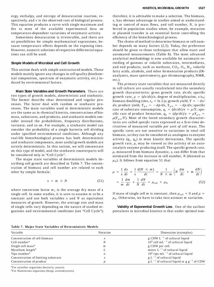
The primary state variables that are measured directlyin cell culture are usually recalculated into the secondarygrowth characteristics: gross growth rate, dx/dt; specificgrowth rate, l � (dx/dt)/x; degree of multiplication, x/x0;biomass doubling time, td � ln 2/l; growth yield, Y � �dx/ds; product yield, Yp/s � �dp/ds, Yp/x � �dp/dx; specificrate of substrate consumption, qs � (ds/dt)/x � l/Y; spe-cific rate of product formation, qp � (dp/dt)/x � lYp/x �l(Yp/x/Y). Most of the listed secondary growth character-istics are called specific rates expressed as a first-time de-rivatives of measured variable per unit of cell mass. Thespecific rates are not sensitive to variations in total cellbiomass, so they can be considered as analogous to enzymeactivity (qs, qp) in most kinetic derivations. The specificgrowth rate, l, may be viewed as the activity of an auto-catalytic enzyme producing itself. The specific growth rate,l, measured from biomass dynamic, x, can differ from thatestimated from the increase in cell number, N (denoted aslN). It follows from equation 51 that
1 dx 1 d(N � m) 1 dm dNl � � � N � m� �x dt x dt N � m dt dt
1 dm 1 dN� � � l � l (52)cell Nm dt N dt
If mass of single cell m is constant, then lcell � 0 and l �lN. Otherwise, we have to take into account m variation.
Validity of Exponential Growth Low. One of the earliestpostulates in microbial kinetics is that under optimal non-

1528 KINETICS, MICROBIAL GROWTH
Table 8. Methods Used for Determination of Microbial Biomass
Method Measuring principle DL Advantage Disadvantages
Dry mass Mass of separated and driedsolids
50 Provides direct unconditionalestimate
Interference from dead cells andnoncell solids
Wet mass Mass of separated material 50 Simplicity, quickness The variation of wet biomassbulk density
Wet biovolume Linear dimension of pelletedcells or colony
100 Simplicity, quickness The variation of wet biomassbulk density
Particulate organiccarbon
CO2 after cell separation andcombustion
1.0 High precision and sensitivity,provides direct estimate ofmass
Interference from dead cells andnoncell solids
Biuret proteins Colorimetric reaction ofpeptide bonds
1.0 High uniformity Variation of protein-to-biomassratio, possible extracellularaccumulation
Folin-Ciocalteuprotein
Colorimetric reaction oftyrosine and tryptophan
0.1 High sensitivity Variation of protein-to-biomassratio and amino acidcomposition of cell protein,possible extracellularaccumulation
DNA Colorimetric estimation ofdeoxyribose
1.0 High specificity, constancy ofthe DNA cellular content
Possible extracellularaccumulation
ATP Bioluminescence assay 10�5 High sensitivity and specificity Variation of the intracellularATP pool
Fatty acids Gas or liquidchromatography,colorimetric reaction
1.0 High specificity, allowsidentification of compositionof mixed culture
Variation of the intracellularcontent, possible extracellularaccumulation
Metabolio potential Rate of added substrateuptake or productformation
10�3–10 High specificity, quickness Variation in conversion factorfrom measured rate tobiomass
Opacity Light scattering 0.1 Simplicity, quicknerss,automation
Interference from noncell solids,cell aggregation, wall growth
Electricalmeasurements
Conductivity 1 Simplicity, quickness,automation
Variation of conversion factor,interference from electrolytesin the medium
Manual microscopy Cell count, measuring ofhypha length
10�5 Low cost, sensitivity, allowsvisual assay ofbiomorphological structure
Time-consuming, low precision
Image analysis Computer-aided count 10�5 Combined benefit of manualand automated quantification,speed, generation of sizedistribution
High cost
Coulter counter Automated count and sizing 10�5 Quickness, automation,generation of size distribution
Interference from noncell solids
Plating Growing of the colonies onPetri dish
10�5 Low cost, high sensitivity Time consuming, low precision
Note: DL � detection limit, the minimum CDW required for an estimation with an error �2% (mg).
restrictive conditions (nutrient media containing all essen-tial components at nonlimiting concentrations, absence ofinhibitors, adequate physicochemical parameters, perfectmixing), the increase in biomass (dx) during an infinitelysmall time interval (dt) is proportional to this time intervaland the instant biomass concentration (x), that is
dx � lxdt
or
dx/dt � lx (53)
where l is the proportionality coefficient. If l is constant,integration of equation 53 gives
lnx � lnx � lt ⇒ x � x exp(lt) (54)0 0
where x0 is biomass at zero time or inoculum size.According to early views, true exponential growth oc-
curs only in the case of symmetrically dividing bacteriawith equal probability of subsequent division for themother and daughter cells. Organisms with asymmetricalmultiplication (budding yeasts) were thought to obey theexponential low only approximately, whereas the growthof filamentous organisms (fungi, streptomycetes) was de-viated considerably. However, direct measurements per-formed from 1930 to 1960 (5) revealed that exponentialgrowth does occur in all prokaryotes and eukaryotes in-dependent of their biomorphological features, includingprotozoa, fungi, and homogeneously cultivated plant and
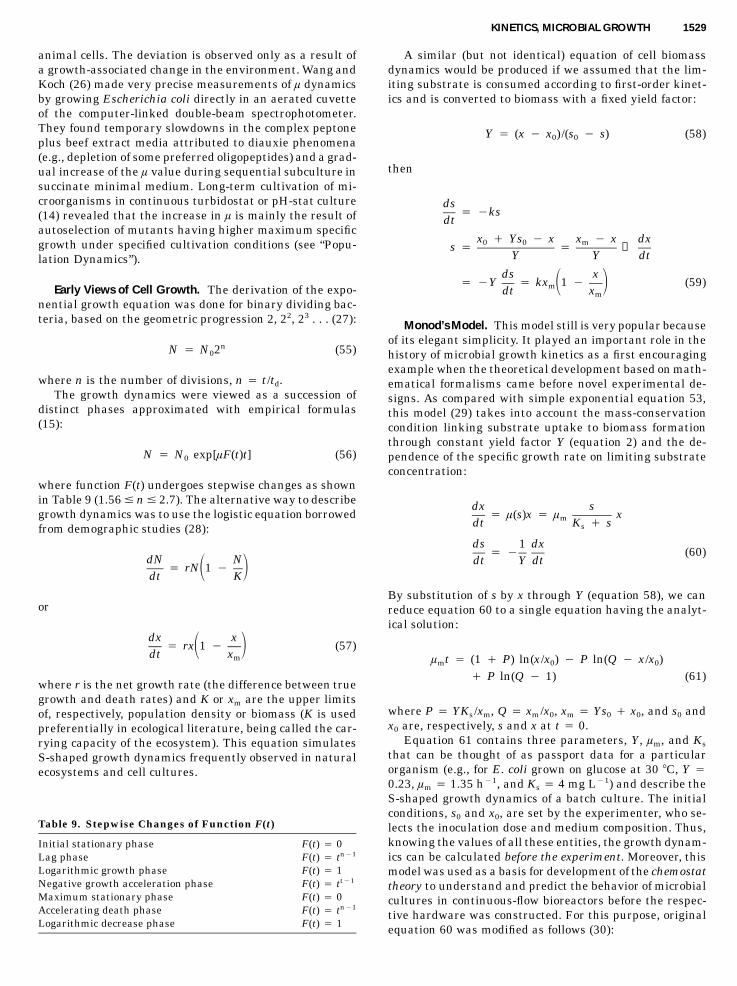
KINETICS, MICROBIAL GROWTH 1529
Table 9. Stepwise Changes of Function F(t)
Initial stationary phase F(t) � 0Lag phase F(t) � n�1tLogarithmic growth phase F(t) � 1Negative growth acceleration phase F(t) � t�1tMaximum stationary phase F(t) � 0Accelerating death phase F(t) � n�1tLogarithmic decrease phase F(t) � 1
animal cells. The deviation is observed only as a result ofa growth-associated change in the environment. Wang andKoch (26) made very precise measurements of l dynamicsby growing Escherichia coli directly in an aerated cuvetteof the computer-linked double-beam spectrophotometer.They found temporary slowdowns in the complex peptoneplus beef extract media attributed to diauxie phenomena(e.g., depletion of some preferred oligopeptides) and a grad-ual increase of the l value during sequential subculture insuccinate minimal medium. Long-term cultivation of mi-croorganisms in continuous turbidostat or pH-stat culture(14) revealed that the increase in l is mainly the result ofautoselection of mutants having higher maximum specificgrowth under specified cultivation conditions (see “Popu-lation Dynamics”).
Early Views of Cell Growth. The derivation of the expo-nential growth equation was done for binary dividing bac-teria, based on the geometric progression 2, 22, 23 . . . (27):
nN � N 2 (55)0
where n is the number of divisions, n � t/td.The growth dynamics were viewed as a succession of
distinct phases approximated with empirical formulas(15):
N � N exp[lF(t)t] (56)0
where function F(t) undergoes stepwise changes as shownin Table 9 (1.56 � n � 2.7). The alternative way to describegrowth dynamics was to use the logistic equation borrowedfrom demographic studies (28):
dN N� rN 1 �� �dt K
or
dx x� rx 1 � (57)� �dt xm
where r is the net growth rate (the difference between truegrowth and death rates) and K or xm are the upper limitsof, respectively, population density or biomass (K is usedpreferentially in ecological literature, being called the car-rying capacity of the ecosystem). This equation simulatesS-shaped growth dynamics frequently observed in naturalecosystems and cell cultures.
A similar (but not identical) equation of cell biomassdynamics would be produced if we assumed that the lim-iting substrate is consumed according to first-order kinet-ics and is converted to biomass with a fixed yield factor:
Y � (x � x )/(s � s) (58)0 0
then
ds� �ks
dt
x � Ys � x x � x dx0 0 ms � � ⇒Y Y dt
ds x� �Y � kx 1 � (59)m� �dt xm
Monod’s Model. This model still is very popular becauseof its elegant simplicity. It played an important role in thehistory of microbial growth kinetics as a first encouragingexample when the theoretical development based on math-ematical formalisms came before novel experimental de-signs. As compared with simple exponential equation 53,this model (29) takes into account the mass-conservationcondition linking substrate uptake to biomass formationthrough constant yield factor Y (equation 2) and the de-pendence of the specific growth rate on limiting substrateconcentration:
dx s� l(s)x � l xmdt K � ss
ds 1 dx� � (60)
dt Y dt
By substitution of s by x through Y (equation 58), we canreduce equation 60 to a single equation having the analyt-ical solution:
l t � (1 � P) ln(x/x ) � P ln(Q � x/x )m 0 0
� P ln(Q � 1) (61)
where P � YKs/xm, Q � xm/x0, xm � Ys0 � x0, and s0 andx0 are, respectively, s and x at t � 0.
Equation 61 contains three parameters, Y, lm, and Ks
that can be thought of as passport data for a particularorganism (e.g., for E. coli grown on glucose at 30 �C, Y �0.23, lm � 1.35 h�1, and Ks � 4 mg L�1) and describe theS-shaped growth dynamics of a batch culture. The initialconditions, s0 and x0, are set by the experimenter, who se-lects the inoculation dose and medium composition. Thus,knowing the values of all these entities, the growth dynam-ics can be calculated before the experiment. Moreover, thismodel was used as a basis for development of the chemostattheory to understand and predict the behavior of microbialcultures in continuous-flow bioreactors before the respec-tive hardware was constructed. For this purpose, originalequation 60 was modified as follows (30):

1530 KINETICS, MICROBIAL GROWTH
dx� (l � D)x
dt
sl � l xm K � ss
ds 1� D(s � s) � lxrdt Y
FD � (62)
V
where sr is the concentration of limiting substrate in thefed-fresh medium delivered with pump from reservoir, F isthe pumping rate (cm3/h), V is culture volume (cm3), andD is the dilution rate defined as the ratio D � F/V, h�1.
The mathematical analysis of equation 62 allows us tomake the following conclusions on the growth kinetics ofcontinuous culture:
1. The described open system attains stable steadystate when dx/dt � 0, ds/dt � 0, and variables x ands are not changed with time (denoting steady-stateconcentrations x and s, respectively). From the firstequation in equation 60, it follows that l � D, thatis, the specific rate of microbial growth is equal tothe dilution rate, which is under the full control ofthe experimenter. From the second equation, we find
x � Y(s � s) (63)0
As compared with Y expression for batch culture(equation 58) the formula in equation 63 no longercontains the term, x0, the inoculum size. Thus, asteady-state culture is not dependent on past history,and its properties are determined solely by currentcultivation parameters.
2. The dilution rates permitting stable microbialgrowth (i.e., those D, at which x � 0) are confinedbetween 0 and washout point or critical dilutionrate Dc
D � l s /(K � s ) (64)c m r s r
3. The specific growth rate l does not depend on eithers0 or x and is governed solely by the substrate con-centration in the cultural liquid. On the other hand,the indirect effect of s0 on l may be evaluated fromthe dependence of x on D, as soon as x and s arelinked by the conservation condition in equation 62.
The most important biological implication of the che-mostat theory was the discovery of the fact that microor-ganisms can grow endlessly with any rate between 0 andlm. Such substrate-limited growth is nevertheless expo-nential, because two subsequent acts of cell division willbe separated by a constant time interval. Earlier, substratelimitation had been observed only transiently at the endof the exponential phase of batch growth. The most impor-tant biotechnological implication of the chemostat modelwas the concept of controlled cell biosynthesis, which im-plies the purposeful manipulation of microbial culture to
optimize the productivity by such tools as changing theflow rate and the composition of medium in continuous-flow bioreactors.
Derivation of the Monod Equation from Mechanistic Con-siderations. The equation relating l and s is known as theMonod equation:
sl � l (65)m K � ss
It was introduced by the author as a purely empirical re-lationship resembling adsorption isotherm. However,many microbiologists did view the Monod equation assomething having deep inherent meaning rather than asjust an empirical formula. Below, we shall outline a num-ber of attempts to deduce this equation logically from theconjectured growth mechanisms.
1. The bottle-neck concept. There is an obvious similar-ity between the Monod and Michaelis-Menten equations.A theoretical substantiation for this similarity can be thebottleneck postulate originally put forward by Blackman(31). According to this postulate, the growth rate of a cellis determined by a single enzymatic master reaction. Mi-crobial metabolism is symbolized as a unidirectional chainof reactions of substrate S conversion to cell biomass X� viasome hypothetical intermediates P1, P2 . . . Pn (32):
k k k k1 2 n n�1
S � X� r P r P r . . . r P r 2X� (66)1 2 n
Assuming steady state in respect to intermediate concen-tration pi, dpi/dt � 0, we arrive at the Monod equation,composite parameters lm and Ks being expressed via ele-mentary kinetic constants of individual enzymatic reac-tions:
dx s� l xmdt K � ss
1l �m n�1
1/k� ii�2
1k � (67)s n�1
k 1/k1 � ii�2
where x � x� � p1 � . . . pn. The bottleneck idea can nowbe formulated as follows. If one of the constants kj � ki, i� 2, . . . , n � 1, i � j, then lm � kj and Ks � kj /k1, and sothe jth enzymatic reaction is the master reaction.
The obvious shortcomings of the reaction scheme inequation 66 are the unjustified oversimplification of thecell metabolism (which is a network, rather than a simpleunidirectional sequence of reactions) and the lack of a def-inite interpretation of variables x� and p in real biochem-ical terms. An evaluation of the characteristic times of ma-jor intracellular metabolic reactions showed that therecould be two possible bottlenecks: uptake of limiting sub-
KINETICS, MICROBIAL GROWTH 1531
strate (processes of active transport, transphosphorylationof sugars etc.) (33) and the formation of intracellularprotein-synthesizing structures such as rRNA and the ri-bosomal proteins (34).
2. Stochastic considerations. Microbial populationswere assumed to consist of active (which utilize the sub-strate) and inactive cells (35). The probability of a transi-tion from the inactive state to the active one was supposedto be proportional to s, whereas the probability of the re-verse transition was s independent. From these assump-tions, a relationship between l and s can be inferred, simi-lar to equation 65.
3. Derivations based on mechanistic considerations ofprotein synthesis (36). The rate of protein synthesis, dp/dt, is supposed to be determined by rRNA concentration Rand by the size of the amino acids pool, A, dp/dt � kxRA/(KA � A), k � constant. Other conditions are defined as R� R0 � (Rm � R0)l/lm, A � bs, and P � p/x, where Rm
and R0 are, respectively, the upper and lower limits of Rvariation, and P and b are constants. For a steady-statechemostat culture, dp/dt � 0 and dx/dt � (1/P)(dp/dt) �0, then
l � (kR /P)s/(R K /br � s) � l s/(K � s) (68)m m A 0 m s
Here again, the Monod equation is derived through a con-sideration of underlying intracellular processes. Needlessto say, none of the cited derivations are free from criticism.The Monod equation remains empirical. Any attempts toprovide the mechanistic interpretation of this equation in-evitably lead to much more complicated mathematical ex-pressions (see late section on structured models).
Biological Meaning and Experimental Determination ofGrowth Parameters Ks and lm. The parameter lm, maximalspecific growth rate, has very lucid biological meaning: itis the upper limit of l variation on specified nutrient me-dium. It could not be attained in reality because of its as-ymptotic nature: l r lm as s r �. However, in practice lm
is achieved if s � Ks. It should be remembered that lm isnot absolute maximum of growth rate, because it dependson the nature of the limiting substrate. For example, E.coli has lm above 2.5 h�1 on complex beef-extract mediumand below 1.0 h�1 on minimal medium with succinate. Sat-uration constant Ks could be defined functionally as suchconcentration of limiting substrate that provides a specificgrowth rate equal to 0.5 of lm. We can say also that Ks isa measure cell affinity to substrate: the lower is Ks thebetter the organism is adapted to consume substrate fromdiluted solution. Any other definitions are speculative, e.g.,Ks interpretation as the dissociation constant of ESC of thecellular enzyme involved in the first step of substrate con-version.
There are several ways to determine numeric values ofKs and lm:
1. Batch culture, differential form of Monod equation.The biomass dynamics, x(t), are followed from the start ofthe exponential phase until the complete consumption ofthe limiting substrate and the attainment of the maximal
cell density, xm. The residual substrate concentration, s iscalculated from mass balance (equation 58); yield is cal-culated as (xm � x0)/s0; the s0 value should be known) andcorresponding l(t) values from the slopes d(lnx)/dt. Finally,parameters Ks and lm (equation 65) are to be found graph-ically or from nonlinear regression as in the case of theMichaelis-Menten equation (see later text).
2. Batch culture, ignoring the substrate uptake. The in-oculum size, x0, and the duration of experiment are chosento minimize the uptake of added substrate s � s0 (37). Typ-ically, bacterial cell density should be of the order 10�5 orless, and it is measured by such sensitive instruments asthe Coulter counter. The quasi-steady-state growth rate ismeasured at several s0 values and then fitted to equation65 as described before. In numerous determinations madeat high cell densities (when we can no longer neglect sub-strate consumption), it was observed that dependence of lduring exponential growth phase on s0 is formally de-scribed by the Monod equation with s replaced by s0 (38).The explanation of these results could be made only bymore complex structured models; however, the describedprocedure is not appropriate for Ks and lm determination.
3. Batch culture, integral form of equation 61. The S-shaped curve of biomass dynamics is fitted directly toequation 61 through either preliminary linearization ornonlinear regression (preferential). Sometimes (e.g., whencells are grown in opaque media) it is more convenient tofollow the dynamics of residual substrate s(t) or productformation p(t), for example, CO2 evolution or dynamics ofO2 uptake (respiration). In these cases, we can integratethe set of differential equation 60 in terms of s(t) or p(t)dynamics, taking into account mass–balance relationshipsin equations 7, 8, and 58 and similar equations.
4. Steady-state chemostat culture. The chemostat pro-vides the opportunity for estimations under steady-statecondition, which is commonly believed to be more reliable.By running an experiment at different dilution rates, D,the corresponding s values may be measured and the de-pendence of l � D on s obtained; in principle, this can bedone as accurately and carefully as desired. Such an ap-proach, however, may and frequently does encounter se-rious technical problems because of the high affinity to lim-iting substrate of some microorganisms. There is a need to(1) select highly sensitive analytical techniques to measureextremely low residual concentrations of particular sub-stances; (2) develop instant sampling procedures to mini-mize substrate loss, and (3) eliminate apparatus-relatedartifacts such as nonperfect mixing and fluctuations in nu-trient medium supply. This can be accomplished by use ofradiolabeled substrate, and other tips are covered in spe-cific experimental works (39,40). However, the most essen-tial objection to this method is that organisms at varioussteady states do change their kinetic properties, which isnot accounted by Monod’s model (see “Structured Models”).
5. Non-steady-state chemostat culture. The measure-ments are made during short-term experiments started byaddition of different amounts of limiting substrate to asteady-state chemostat culture. Then, substrate uptake orrespiration rates are recorded in perturbed culture until
1532 KINETICS, MICROBIAL GROWTH
the new steady state is established (2). The opportunity ofcontinuous culture is that the physiological state of cellsjust before perturbation is well defined and reproducible.On the other hand, these experiments do provide data onaffinity to substrate (Ks) and maximal rates of respiration(e.g., or uptake Qs, which are related but are not iden-QCO2
tical with lm):
l � Y Q � Y Q (69)m p/x CO s/x s2
where stoichiometric parameters Yp/x � dp/dx and Ys/x �ds/dx should be determined in independent experiments.Immediate assay of lm in such an experimental setup ispossible as follows: the steady state is perturbed by settingthe dilution rate by 20 to 100% higher than the criticalvalue Dc (equation 64). The washout dynamics are followedand lm is determined from approximate relationship (5): x� x(0) exp[(lm�D)t], where x(0) is biomass before pertur-bation. More rigorous estimate of lm could be provided ifsuch washout experiments were made at several (at leasttwo) input substrate concentrations s0 to account for thefact that sr is still not infinity.
Modification of the Monod Equation. It was found thatnot all experimental data could be reasonably well fittedby equation 65. The best-fit hyperbola often passed aboveexperimental points at small s and below them at large s.A better fit was claimed to be provided by using the follow-ing, entirely empirical, equations:
l � l [1 � exp(�Ks)] (70)m
n nl � l s /(K � s ) (71)m s
l � l s/(K x � s) (72)m s
The preference of the first expression, equation 70 (41), isquestionable. An expansion of Monod equation by additionof the third parameter, n in equation 72 (42), or introduc-tion of the second variable, x in equation 71 (43), does im-prove the approximation capability of kinetic equations.We can even provide the mechanistic basis for this im-provement. Thus, the Moser equation (equation 71) is simi-lar to the Hill equation in enzymology (equation 43), in-dicating the cooperativity effects in performance of somemaster reaction of cellular metabolisms. The Contois equa-tion (equation 72) could be interpreted in terms of growthautoinhibition by-products, because under the realistic as-sumptions (x � x0, xYp/x/Kp � 1 and product p formationcoupled with growth), the apparent saturation constant
is almost proportional to accumulated biomass x:appKs
appK � K (1 � p/K ) � K [1 � Y (x � x )/K ] � K xs s p s p/x 0 p s
(73)
An Account of Maintenance Requirements. Powell (44)assumed that substrate uptake rate q obeys the Michaelis-Menten kinetics; then, from mass–balance equation 18 itfollows that
mq � Q /(K � s) � l/Y � m (74)s s s
If lm is defined as lm � YQs (5), then
ml � l s/(K � s) � mY (75)m s
If we define lm � Ym(Qs � m) (2), then
l � l (s � s*)/(K � s)m s
ms* � K mY /l (76)s m
Equations 75 and 76 both predict the occurrence of thresh-old substrate concentration s*, below which growth is im-possible. It yields a substantially better fit to experimentaldata. The difference is that according to equation 75, theparameter lm is the specific growth rate under imaginaryconditions of zero maintenance requirements, whereasequation 76 implies the traditional definition of lm as thespecific growth rate under substrate excess: l r lm whens r �.
Account for Substrate Leakage. Mathematically identi-cal to equation 76, a modification of the Monod equationwas proposed for the case of conserved substrates. How-ever, the biological meaning is entirely different: if the spe-cific leakage rate is assumed to be constant, then a de-crease in s down to some threshold value s* will lead to thecounterbalance of the two reverse processes (uptake andleakage), so that the net consumption of the limiting sub-strate will be zero.
Account of Inhibitory Effects. A few valuable refine-ments of the Monod equation were borrowed from enzy-mology; most often they were noncompetitive and sub-strate inhibition. The former inhibition mechanism is bythe so-called Monod-Ierusalimsky equation:
s Kpl � l � (77)m K � s K � ps p
The growth retardation with an excess of such substratesas phenol, methanol, and ethanol is described by an ana-logue of Haldane’s equation (45):
sl � l (78)m 2K � s � s /Ks ss
Equation 78 simulates a single-peak curve, and so thesame l value may be obtained at two different s, one in thesubstrate-limiting range, dl/dt � 0 (stable), and the otherin the substrate inhibition range, dl/dt � 0 (unstable). Asustainable maintenance of a population under conditionsof substrate inhibition is possible either in the second stageof a two-stage chemostat or in the case of plentiful wallgrowth in a conventional chemostat (46).
Account of Diffusion Effects. We will present one ex-ample of such models (44). The basic assumption is thatsubstrate is taken up by an enzyme that obeys Michaeliskinetics and is localized on the inner side of cell membrane.The actual substrate concentration around the enzyme-active centers is smaller than in the solution, because of alimited diffusion rate. By applying a simplified Laplaceequation, it was found eventually that
KINETICS, MICROBIAL GROWTH 1533
l (K � L � s) 4Lsm sl � 1 � 1 �� 2��2L (K � L � s)s
s� l (79)m K � L � ss
where L is a factor determined by membrane permeabilityand by the maximum rate of the enzymatic reaction.
Structured Models
The unstructured models (such as Monod’s model or itsmodifications) are able to predict and describe only sim-plest manifestation of growth phenomena. Sometimes it isdeclared that Monod-type models are able to describe onlybalanced and steady-state growth. The analysis of morecomplicated unbalanced and non-steady-state growth re-quires formulation of structured models.
Definitions. Balanced growth was defined by Campbell(47) as a proportional increase in the amounts of all cellcomponents, in other words, balanced growth producescells of the same quality without any variation of compo-sition. The terms steady state and non steady state stemfrom chemical and enzyme kinetics. The first one refers tosuch a regime when the reaction rate remains constantbecause of an exact balance between formation and break-down of intermediary products such as the enzyme–substrate complex. In microbial culture, the growth iscalled steady state if specific rather than total rates remainconstant. In an open system, such as a chemostat, bothtotal (dx/dt, ds/dt) and specific rates (l � (1/x)dx/dt, qs �(1/x)ds/dt) tend to have constant steady-state values. Aclosed system, such as a batch culture, should be consid-ered under steady state only during the exponential phasewhen l and qs are constant. The linear growth with a con-stant total rate (dx/dt � lx � constant) is characterizedby monotonously declining l, and is not steady-stategrowth. However, under some conditions (such as in dial-ysis culture) it may attain quasi steady state, when ds/dt� 0.
The non-steady-state kinetic regimes take place beforeestablishment of steady state or after its perturbation. Inenzyme kinetics, non-steady-state measurements aretaken in the millisecond range of time scale. In microbialcultures, similar non-steady-state transient and pertur-bation processes advance much more slowly, typically dur-ing several hours and days. An example is a transient pro-cess in the chemostat induced by changes in D or sr
(fed-substrate concentration). In such growth, l, qs, qp, andother metabolic rates exhibit continuous variation in time.The attractiveness of non-steady-state studies for micro-biology and biotechnology is obvious:
• They allow a wider range of hypotheses to be testedand yield much more data on the studied objects.
• They have higher practical value; in biotechnology,steady-state operation is the exception rather thanthe common routine because of unavoidable distur-bances in cultivation conditions.
• They provide additional tools for optimal regulationof cell performance in the bioreactor, because pur-
poseful non-steady-state growth may display greaterefficiency and higher productivity (48).
The notions of steady-state and balanced growth areclose but not identical. The first is more strict; steady-stategrowth has to be balanced by definition (otherwise some ofthe specific rates responsible for synthesis of the changedcell component should vary). On the other hand, the bal-anced growth can be for some time nonsteady, perhaps dur-ing the late exponential phase of batch culture when l de-clines while cell composition remains unchanged. Duringlong-term experiments, non-steady-state growth leads in-evitably to a change of cell composition; it becomes unbal-anced. For heterogeneous populations, the situation maybe more complicated. For example, the growth in the sec-ond stage of a two-stage chemostat attains a steady state,and the biomass and residual substrate concentration areconstant. However, such growth is not balanced, becausecells delivered from the first stage differ in their propertiesand composition as compared with the bulk of cells in thesecond stage. This situation was termed the transientsteady state (49).
By structured, we mean mathematical models describ-ing growth-associated changes in microbial cell composi-tion. It includes mass–balance equations for all assignedintracellular components. Their concentrations can be ex-pressed either per unit volume of fermenter vessel (c1, c2,. . . , cn), or per unit cell mass (C1, C2, . . . , Cn), and henceCi � ci/x. The mass–balance equations can be written asfollows
n
c � x� ii�1
n
C � 1 (80)� ii�1
For each variable Ci, a differential equation is written thattakes into account all sources, r�, and sinks, r�, as well asits dilution from cell mass expansion (growth)
dCi� r (s, C , . . . , C ) � r � (s, C , . . . , C ) � lC� 1 n 1 n idt
(81)
The simplest structured models with n no more than 2or 3 are called two- or three-compartment models. For ex-ample, a model (50) incorporated two compartments: nu-cleic acids and proteins combined with other active cellcomponents. The model variables also included concentra-tions of the limiting substrate and the inhibitor. Comparedto Monod’s model, the proposed set of four equations wasable to account for a much wider range of dynamic pat-terns. Specifically, it simulated D-dependent changes inthe cell composition (chemostat) and all known growthphases of batch culture from the lag to decline. However,the choice of variables in this model was more or less ar-bitrary, so it should be regarded more as a bright illustra-tion rather than a research tool.
During the past decade, much more realistic structuredmodels based on biochemical data have been developed.
1534 KINETICS, MICROBIAL GROWTH
The simulation model of E. coli growth (51) contains thefollowing dynamic variables: glucose and , as exosub-�NH4
strates; CO2 and acetate, as products excreted into the me-dium; amino acids; ribonucleotides; deoxyribonucleotides;monomeric precursors of cell wall components; rRNA andtRNA; nonprotein polymeric components; glycogen; guano-sinetetraphosphate; enzymes transforming ribonucleo-tides into deoxyribonucleotides; ATP; NAD(H); and pro-tons. Altogether, the dynamic model amounts to a systemof 21 differential and 14 algebraic equations. An even morecomplicated model simulating growth of Bacillus subtilis(52) is the set of 39 nonlinear and coupled differentialequations containing nearly 200 parameters! These mod-els are able to simulate particular growth features such aschanges in cell sizes, shape, and composition as well as theD-dependent variations in replication time brought aboutby the shifts in glucose concentration. However, the pre-dictive capability of such an intricate dynamic modelshould be still estimated as modest as compared with in-vested modeling efforts; they are still nothing more than a“caricature parody” of microbial biochemistry and are toocomplex to be studied by conventional mathematical tools(stability analysis, parameters identification, etc.) or to beused in biotechnological applications. The best choice of amathematical model lies, apparently, midway between un-structured and highly structured models outlined here.One of the known compromises has been found throughattempts to express quantitatively the cell physiologicalstate.
Physiological State of Chemostat Culture. The term wascoined by Malek (53) without giving a clear definition. Theimpetus for the development of the concept of a physiolog-ical state was the evidence on changes in the chemical com-position of microorganisms as dependent on dilution rateD and medium composition in chemostat culture (54). Ithas been found that some of the studied parameters re-mained constant (content of cell DNA and carbon) whileothers exhibited regular D-dependent variations, either anincrease (RNA content, cell sizes) or a decrease (the con-tent of reserved polysaccharides). Those properties thatwere D dependent were recognized as components of thevector of the physiological state.
Powell (44) combined and put on a quantitative math-ematical footing three notions, which were beforehandseparated and cloudy: (1) physiological state, (2) past his-tory, and (3) non-steady-state growth kinetics of microbialculture. The specific rate of substrate uptake, qs, was pre-sented as a product
q (s) � q�(s)S(s) (82)s a
where S(s) is a simple saturation function (e.g., a Michaelishyperbola), S(s) � s/(Ks � s), and is a function asso-q�(s)a
ciated with the microbial physiological state. The instantvalue of is determined by way in which s varies untilq�(s)a
the given moment (s h ago), effects of later events contrib-uting more than earlier ones. Transient processes are in-fluenced by the past history of the culture in the followingmanner. Suppose that steady-state growth of a chemostatculture is upset and the residual substrate concentration
jumps from s(0) to s(1). Immediately, qs will increase fromQ(0)S[s(0)] to Q(0)S[s(1)]. If no further changes in s(1) oc-cur, then Q will also eventually attain a new steady-statevalue equal to . In essence, Q is the potential met-q�[s(1)]a
abolic activity, that is, the specific rate of a key metabolicprocess measured just at the moment of relief from sub-strate limitation. The transient Q dynamics are describedas net change equals production minus dilution caused bycell growth:
dQ� r(Q, s) � l(Q, s)Q (83)
dt
Substance Q may, in reality, be represented by a singleenzyme or multienzymatic complexes as well as by ribo-somes or other cell components occupying the bottleneckposition. Monod’s model, supplemented by equation 83,made possible at least a qualitative understanding ofchemostat-transient processes triggered by a D switch(55).
The synthetic chemostat model (SCM) (2) combines Pow-ell’s ideas with the routine of conventional structured mod-els. This model is similar to the cybernetic model (56,57).The basic SCM interprets microbial growth as a conversionof exosubstrate S into cell macromolecules X� via a pool ofintermediates L:
S L X'
CO2
Transport qs
Leakage v
Synthesis qL
Turnover a
Cell wall
Macromolecular cell components are susceptible to degra-dation (turnover), and monomeric metabolites can escapeinto environment because of leakage. Contrary to simplechemical catalysts, the composition of end product X� is notuniform and varies in response to a changing environmentbecause of the adaptive nature of microbial metabolism. Atthe heart of the SCM are the solution of the problem, howto cope with these variations, and how to describe adaptivechanges in cell composition by relative simple models.
All macromolecular cell constituents are divided intotwo groups: primary cell constituents necessary for inten-sive growth (P components), and components needed forcell survival under any kinds of growth restriction (U com-ponents). The characteristic examples of P components areribosomes (rRNA and ribosomal proteins) and enzymes ofthe primary metabolic pathways. Their intracellular con-tent increases parallel to an increase in l. The contributionof U components to cell biomass decreases with growth ac-celeration. Examples are enzymes of the secondary metab-olism, protective pigments, reserved substances, andtransport systems of high affinity.
The analysis of available data as well as mass-conservation conditions allowed the formulation of severalrules of variation of cell components taking place becauseof optimal control of cell biosynthesis:
1. Amounts of P and U components expressed as a frac-tion of total cell mass (P and U, gram per gram of

KINETICS, MICROBIAL GROWTH 1535
Bio
mas
s, r
esid
ual s
ubst
rate
, m
g L–1
RN
A c
onte
nt, fr
acti
on o
f C
DW
Time (h)–10 –5 0 5 10 15 20 25 30 35 400
2
4
6 32
1
8 0.16
0.12
0.08
0.04
0
Figure 7. SCM simulation of transient growth induced by changeof chemostat dilution rate. Residual glycerol concentration (1), bio-mass (2), and cell RNA content (3). At t � 0, dilution rate wasshifted from 0.004 to 0.24 h�1. Source: Redrawn from Ref. 2; theoriginal data (59) are for chemostat culture of Aerobacter aero-genes limited by glycerol.
Mas
s fr
acti
on o
f ce
ll co
mpo
nent
s
Chemostat dilution rate, D (h–1)0.0 0.2 0.4 0.6 0.8 1.0
0.0
0.2
0.4
0.6
0.8
Lipids DNA
RNA
Polysaccharides
Proteins
1.0
Figure 6. Simulation of D-dependent changes in cell compositionof Aerobacter aerogenes grown in -limited chemostat culture.�NH4
The curves are calculated from SCM (2), and the original experi-mental data are from Ref. 58.
biomass respectively) vary within the upper (Pmax,Umax) and low (Pmin, Umin) limits, the latter being theconstitutive part.
2. An increase of one individual P component is accom-panied by increase of other P components.
3. The total enlargement of Psum is accompanied by cor-responding decrease of Usum and vice versa.
4. The P/U ratio is controlled by the limiting substrateconcentration in an environment.
These rules are translated into mathematical terms asfollows:
min minP � P P � P1 1 n n�•••� � rmax min max minP � P P � P1 1 n n
min minU � U U � U1 1 m m�•••� � 1 � rmax min max minU � U U � U1 1 m m
sr � (84)
K � sr
where variable r (index of physiological state) is alreadyscalar (not vector!) function controlled by environmentalfactors (e.g., concentration of the limiting substrate). Ther value in steady-state chemostat culture changes fromzero (in culture at almost zero growth rate, when s r 0 andall P components come down to low limits) to 1.0 (in unlim-ited culture, when s r � and P components attain maxi-mum). During transients caused by sudden s changes, aninstant r value goes toward new steady state (comparewith equation 82):
dr s� l � r (85)� �dt K � sr
The introduction of the r variable greatly simplifies theuse of structured models because the adaptive variation ofcell composition (and metabolic activity, which is deter-mined by the intracellular content of particular enzymes)now could be expressed via one single master variable r.For example, the specific rate of substrate uptake qs is de-fined as:
Qs Q�sq � r � (1 � r) (86)s K � s K� � ss s
where the first and the second terms on the right sidestand, respectively, for low (P component) and high (U com-ponent) affinity of transport system. Similar r-dependentexpressions are derived for other reactions (qL, v, a) andstoichiometric parameters.
Predictive and clarifying capabilities of SCM turned outto be higher than more complex structured models. Con-trary to all known chemostat models, SCM provides ade-quate simulation of D-dependent variation of the microbialphysiological state. Under energy- and C-limited growth,it was expressed as an increase of apparent Ks, potentialuptake and respiration rates, maintenance ration, andturnover parallel to increase of D. Under N limitation, a
similar trend was complemented by considerable decreaseof YN due to alteration of cell composition in favor of N-richP components (Fig. 6). SCM adequately describes the tran-sient growth caused by shift-up in chemostat culture. Thephenomena of overshoot in substrate concentration andundershoot in biomass during transient growth are ex-plained by slow adjustment of cell composition (RNA con-tent, respiratory activity) to new growth conditions (Fig.7). Batch culture limited by carbon and energy source wassimulated by SCM on the whole from inoculation to deathstage; conventional growth phases (lag, exponential, de-celeration, stationary, decline) were generated automati-cally without setting any specific conditions (Fig. 8). It isimportant that SCM realistically describes and predictsnot only net growth but also the survival dynamics ofstarving cells after substrate depletion. During this phase,

1536 KINETICS, MICROBIAL GROWTH
Res
idua
l glu
cose
(m
g L–1
)
Time (h)0 5 10 0 200 400 600 800
0
50
100
150
1 12
2
200 160
120
80
Bio
mas
s (m
g L–1
)
40
0
Figure 8. SCM simulation of complete dynamic curve of batchculture; residual glucose (1) and biomass (2) of yeasts Debaryomy-ces vanrijiae (old name D. formicarius) grown on glucose-mineralmedium (2). Note that contrary to old empirical models (equation56), all growth phases are reproduced automatically without spec-ifying preset time ranges.
surviving bacteria sustain very slow cryptic growth at theexpense of cell turnover and L leakage. The rate of declinein biomass gradually decreases as the result of buildup ofsome U components (parallel to the decrease of such P com-ponents as RNA and CN-sensitive respiration enzymes).Batch culture limited by conserved substrate (the sourceof N, P, Mg, Fe, or other) has an interesting feature: thegrowth is not stopped after substrate depletion but pro-ceeds at an even higher rate. SCM explains this phenom-enon by the partitioning of deficient elements betweenmother and daughter cells.
Cell Cycle
The term cell cycle is used to designate the regularly re-peated sequence of events that occur between consecutivecell divisions, for example, the formation of two identicaldaughter cells from one cell, which takes place in mostknown bacteria. Equivalent cell cycle events include bud-ding (most yeasts and budding bacteria), branching of hy-pha (filamentous organisms), fragmentation (some coccoidand corineform bacteria). The majority of available datahave been obtained for rod-shaped bacteria (E. coli, Sal-monella typhimurium, Bacillus cereus) under steady-stategrowth conditions when the cell cycle consists of three dis-tinct phases:
1. The growth of the newborn cell without chromosomereplication from the initial mass m0 until some criti-cal initiation mass m*
2. DNA replication (C period)3. Separation of daughter cells (D period)
Relationship between Cell Size and Specific Growth Rate.The periods C and D are constant; in E. coli, they occupyabout 40 and 20 min, respectively, independent of environ-mental conditions. However, the duration of phase 1 de-pends on cultivation conditions; the time of the single-cell
mass increase from m0 to m* is inversely related to thespecific growth rate l. It is this difference that yields l-dependent variations of cell sizes, because faster-growingcells produce for the same s � C � D time a larger cellmass than do slower-growing cells. It became clear fromthe following simple algebra.
The steady-state growth of an individual cell proceedsexponentially throughout the entire cell cycle [m � m0 •exp(lt)]. At the time of the second part of the cycle, it takesexactly s min for the cell to enlarge from critical mass m*to 2m0. Hence,
2m � m* � exp(ls) ⇒ m � 0.5m* � exp(ls) (87)0 0
Equation 87 remains valid for steady-state culture at anyl, which can be varied from 0 to lm. Assuming that cellcritical mass m* is constant and does not depend on growthrate, we see that equation 87 predicts a l-dependent vari-ation mass of newborn cells m0 and hence the averagemass and size of the bacterial population. This finding issupported by numerous experimental studies from the be-ginning of this century (60) that displayed the positive cor-relation between cell size and growth rate. Because theterm ls is rather small (ls � ltd � ln 2), it is difficult tonotice the curvature of the experimental curve within themeasurement error. Thus, the relationship between theaverage cell size m (m � m0 � 2 � ln 2 for rod-shapedbacteria; see derivation in equation 88) and l is given asan empirical linear approximation:
m � m(0) � kl (88)
The regression parameters m(0) and k have a meaningfulbiological interpretation: y intercept, m(0) � 2 ln 2 �0.5m* � (ln 2) � m* is equal to approximately 69% of thecell critical mass m* initiating chromosome replication,and slope k � [exp(lms) � 1]/lm � s is close to the durationof C � D periods.
The postulate on the constancy of the critical mass, m*was derived from the observation that the cell has accuratecontrol over its size at division and poorer control over itsage at division (61). Recently, accurate measurements withflow cytometry (62) revealed that m* is inversely relatedto the specific growth rate; slowly growing cells tend toinitiate DNA replication at a slightly higher critical massas compared with intensively growing cells. However, wemay safely assume that m* variation is much smaller thanthe variation of cell mass during the cell cycle: dm*/dt �dm/dt.
Simulation of Cell Cycle by Simple Deterministic Struc-tured Model. In biochemical terms, it is difficult to envis-age how cell mass per se could determine when to initiatereplication. A more likely candidate is some mass-relatedparameter, such as intracellular concentration of some sig-nal metabolite like guanosine tetraphosphate or an initi-ator protein, according to the popular model proposed byHelmstetter and Cooper (63,64). It was postulated that theinitiation of DNA replication is triggered by a thresholdintracellular concentration of this protein V*; this proteinis synthesized at a rate proportional to the total growth
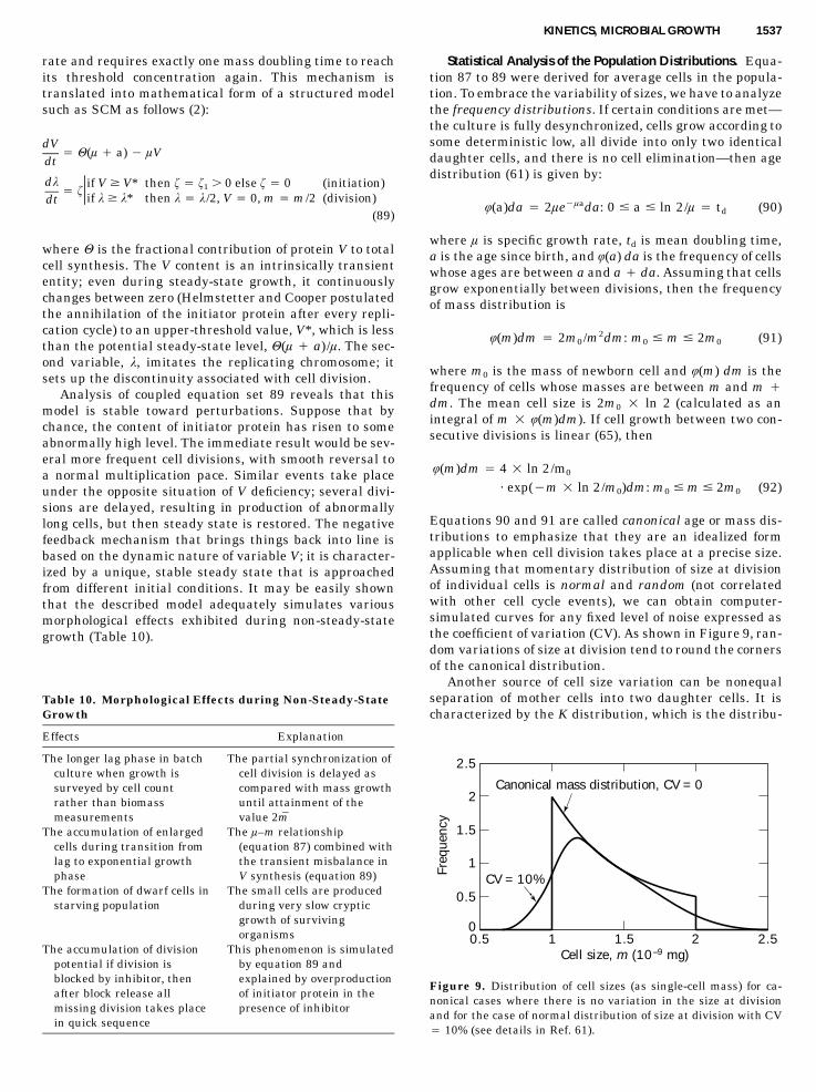
KINETICS, MICROBIAL GROWTH 1537
Freq
uenc
y
Cell size, m (10–9 mg)0.5 1 1.5
CV = 10%
Canonical mass distribution, CV = 0
2 2.50
0.5
1
1.5
2
2.5
Figure 9. Distribution of cell sizes (as single-cell mass) for ca-nonical cases where there is no variation in the size at divisionand for the case of normal distribution of size at division with CV� 10% (see details in Ref. 61).
Table 10. Morphological Effects during Non-Steady-StateGrowth
Effects Explanation
The longer lag phase in batchculture when growth issurveyed by cell countrather than biomassmeasurements
The partial synchronization ofcell division is delayed ascompared with mass growthuntil attainment of thevalue 2m
The accumulation of enlargedcells during transition fromlag to exponential growthphase
The l–m relationship(equation 87) combined withthe transient misbalance inV synthesis (equation 89)
The formation of dwarf cells instarving population
The small cells are producedduring very slow crypticgrowth of survivingorganisms
The accumulation of divisionpotential if division isblocked by inhibitor, thenafter block release allmissing division takes placein quick sequence
This phenomenon is simulatedby equation 89 andexplained by overproductionof initiator protein in thepresence of inhibitor
rate and requires exactly one mass doubling time to reachits threshold concentration again. This mechanism istranslated into mathematical form of a structured modelsuch as SCM as follows (2):
dV� H(l � a) � lV
dt
dk if V � V* then f � f � 0 else f � 0 (initiation)1� f�if k � k* then k � k/2, V � 0, m � m/2 (division)dt(89)
where H is the fractional contribution of protein V to totalcell synthesis. The V content is an intrinsically transiententity; even during steady-state growth, it continuouslychanges between zero (Helmstetter and Cooper postulatedthe annihilation of the initiator protein after every repli-cation cycle) to an upper-threshold value, V*, which is lessthan the potential steady-state level, H(l � a)/l. The sec-ond variable, k, imitates the replicating chromosome; itsets up the discontinuity associated with cell division.
Analysis of coupled equation set 89 reveals that thismodel is stable toward perturbations. Suppose that bychance, the content of initiator protein has risen to someabnormally high level. The immediate result would be sev-eral more frequent cell divisions, with smooth reversal toa normal multiplication pace. Similar events take placeunder the opposite situation of V deficiency; several divi-sions are delayed, resulting in production of abnormallylong cells, but then steady state is restored. The negativefeedback mechanism that brings things back into line isbased on the dynamic nature of variable V; it is character-ized by a unique, stable steady state that is approachedfrom different initial conditions. It may be easily shownthat the described model adequately simulates variousmorphological effects exhibited during non-steady-stategrowth (Table 10).
Statistical Analysis of the Population Distributions. Equa-tion 87 to 89 were derived for average cells in the popula-tion. To embrace the variability of sizes, we have to analyzethe frequency distributions. If certain conditions are met—the culture is fully desynchronized, cells grow according tosome deterministic low, all divide into only two identicaldaughter cells, and there is no cell elimination—then agedistribution (61) is given by:
�lau(a)da � 2le da: 0 � a � ln 2/l � t (90)d
where l is specific growth rate, td is mean doubling time,a is the age since birth, and u(a) da is the frequency of cellswhose ages are between a and a � da. Assuming that cellsgrow exponentially between divisions, then the frequencyof mass distribution is
2u(m)dm � 2m /m dm: m � m � 2m (91)0 0 0
where m0 is the mass of newborn cell and u(m) dm is thefrequency of cells whose masses are between m and m �dm. The mean cell size is 2m0 � ln 2 (calculated as anintegral of m � u(m)dm). If cell growth between two con-secutive divisions is linear (65), then
u(m)dm � 4 � ln 2/m0
• exp(�m � ln 2/m )dm: m � m � 2m (92)0 0 0
Equations 90 and 91 are called canonical age or mass dis-tributions to emphasize that they are an idealized formapplicable when cell division takes place at a precise size.Assuming that momentary distribution of size at divisionof individual cells is normal and random (not correlatedwith other cell cycle events), we can obtain computer-simulated curves for any fixed level of noise expressed asthe coefficient of variation (CV). As shown in Figure 9, ran-dom variations of size at division tend to round the cornersof the canonical distribution.
Another source of cell size variation can be nonequalseparation of mother cells into two daughter cells. It ischaracterized by the K distribution, which is the distribu-

1538 KINETICS, MICROBIAL GROWTH
tion of the ratio of daughter-cell length to mother-celllength. The average values absolutely necessary equals0.5, but CV is at best about 4% (e.g., for well-behaved E.coli strains) and can attain rather high values for otherorganisms. The deviation of observed versus predicted sizedistribution may be caused also by cell death and differentkinds of cell pathology (abnormally long or dwarf cells).
Collins and Richmond (66) introduced an entirely dif-ferent approach based on the use of three distributions:
m m m
v � l{2 Wdm � u(m)dm � k(m)dm}/k(m)m � � �0 0 0
(93)
where vx is the growth rate of cells of size m, k(m) is theextent of population distribution, W is the momentary dis-tribution of dividing cells, and u(m) is the momentary dis-tribution of newborn cells. This equation allows the cal-culation of the mean growth rate of cells of particular sizeclass. Instead of this analytical method, Koch in his workwith Shaechter (61) proposed the synthetic approach.Starting from the set of specific postulates of the cell mul-tiplication mechanism (linear or exponential growth of cellmass between divisions, kind of control, the evenness ofthe division), they derived the size or age distribution,which then was compared with the observations.
The Growth Low. Some believe that there should be ageneral low of cell growth that can be discovered by sen-sitive methods of analysis. The rate of biomass growththroughout the cell cycle was hypothesized to be linear,bilinear, exponential, double-exponential, and so on. Twolimiting cases have generally been considered: the expo-nential and linear growth models proposed, respectively,by Cooper and Kubitschek (57). To differentiate betweenthese two mechanisms, three classes of experiments havebeen used:
1. Size measurements of individual cells growing in themicroculture by use of phase-contrast microscopy orrecently developed confocal scanning light micros-copy combined with image analysis.
2. Pulse-chase labeling of cells with their subsequentseparation into different phases of the cell cycle.Most frequently, labeled uracil and leucine are usedas precursors of RNA and protein synthesis, respec-tively. There are two major sources of errors in thisapproach: poor resolving power of separation meth-ods and artifacts associated with effects of exogenouscompounds on intracellular fluxes (feedback inhibi-tion, pool expansion, label dilution, etc.). One of thebest options for separation is probably the “baby ma-chine,” based on the membrane elution principle(67). To minimize the second source of error, the mu-tants blocked in the synthesis of the probe compoundcan be used.
3. Analysis of the frequency distributions of steady-state populations (see equations 91 and 92). How-ever, the resolving power of this approach is ratherlow because linear and exponential models producesimilar patterns.
Most of the obtained results are in better agreementwith the exponential growth model rather than with thelinear model. However, there are some serious doubtsabout whether there is a unique simple mathematicalgrowth low describing bacterial growth during the divisioncycle. Cooper (67) proposed distinguishing three categoriesof cell components that are synthesized with a unique pat-tern:
1. Cytoplasm (proteins, RNA and ribosomes, small mol-ecules) that is accumulated exponentially.
2. Cell DNA that is replicated in a linear fashion as asequence of constant and zero rates.
3. Cell surface composed of peptiodoglycan and mem-branes that are synthesized exponentially duringmost parts of the cell cycle, but immediately beforecell division the synthesis accelerates to accomplishnew pole formation.
Thus, the growth pattern of the whole cell is the sum ofthese three patterns. Because the cytoplasm is the majorconstituent (up to 80% of CDW), then the growth of the cellshould be approximately exponential.
Population Dynamics (Mutations, Autoselection, PlasmidTransfer)
Description of Mutation and Autoselection. The contin-uous culture turned out to be a very efficient tool to studymutation and autoselection (67). Let N be the total cellconcentration, M the concentration of mutants, l the spe-cific growth rate of the main nonmutated part of the cellpopulation, and g the specific growth rate of neutral mu-tants, then
dM� klN � gM � DM
dt
dN� lN � klN � DN (94)
dt
where k is the mutation rate expressed as the ratio of thenumbers of mutants to total number of cells formed. If k �1 and l � g, in the steady state, we obtain l � g � D, and
dM� kND
dt
or
M � M � kDNt (95)0
If g � l, then the original strain will be displaced by themutant, otherwise, if g � l, M will tend to a lower limitM* � kN/(1 � g/D).
Experimental studies of phage-resistant mutants in atryptophan-limited chemostat culture of E. coli showedthat the period of linear M increase in accordance withequation 95 was fairly short. Every 20 to 100 generationsthere was an abrupt fall in the number of mutants, afterwhich the linear growth resumed at the same rate (67).

KINETICS, MICROBIAL GROWTH 1539
The observed saw-tooth dynamics in M were explained byMoser (43) as a combined effect of mutation and selection.The original wild clone gives not a single but a whole arrayof mutations with subsequent reversions. Let us denote thetotal cell population in a chemostat culture as N, which isthe sum of all subpopulations, including original andemerging variants, N � RNi. All possible transitions be-tween variants are given by the matrix, kirj( j � 1, . . . , n;i � 1, . . . , n; j � i). Then, the chemostat model takes thefollowing form:
n dNdN j� � l(s)N � DN�dt dtj�1
n1l � l N� j jN j�1
n ndNj� l (s)N � DN � k N � k Nj j j � jri j � irj idt i�j j�i
nds� D(s � s) � l (s)N /Y0 � j j jdt j�1
sl (s) � l (96)j m K � ssj
Every drop in the saw-tooth dynamics of neutral mutantsdetected by their phage resistance can be interpreted asthe appearance of other types of spontaneous mutant withhigher growth capabilities. In a chemostat culture, suchmutants overcompete and displace all other cells by virtueof their higher affinity to limiting substrate (a decreasedKs value). Let such a mutant be denoted by the subscriptk and (s) be the average growth rate of all other subpop-l
ulations. The selection pressure for this mutant, r, is givenby
d(M /N) M Mk k k� r � [l (s) � l(s)] (97)kdt N N
If Ksk � Ksj( j � k), then r � 0 until a new equilibrium isestablished. In this process, the original cells will be dis-placed by the mutants and the growth-limiting substrateconcentration will decrease from s1 � DKsj/(lm � D) to s2
� DKsk/(lm � D), and the culture density will rise by Y(s1
� s2).
Autoselection in Turbidostat and pH Auxostat. The affin-ity to substrate was not always the only driving force ofselection outcome. A number of instructive examples werereviewed by Pechurkin (14).
1. In turbidostat and pH auxostat, autoselection is infavor of mutants with higher maximum specific growthrates, r � lmk � lmj � 0. Because the population densityis kept constant instrumentally and the dilution rate isallowed to vary, then autoselection results in the increasein D from lmj to lmk.
2. Mutation toward a higher growth efficiency, Yk � Yj,will lead to the same result as an increase in lm: r � lk �lj � (lmk � lmj)s/(Ksj � s), as soon as lk � qsYk and lj �qsYj.
3. Growth of a mutant with a higher resistance to in-hibitory metabolic products can be described by equation77 with Kpk � Kp. Under selection pressure r � lk � l �lm(s/Ks � s)[Kpk/(Kpk � p) � Kp/(Kp � p)], the originalpopulation will be completely displaced, and the productconcentration will reach a higher steady-state level, p �lmKpks/(Ks � s)D � Kpk.
4. Growth of mutants resistant to an antibiotic will notbe affected by competition if the respective antibiotic iscontinuously supplied: r � lk(s), because l � 0 for allother forms. The dynamics of the total population will begoverned by the initial density of the mutant.
5. A mutation resulting in enhanced adhesion to fer-menter walls will lead to accumulation of slow growingcells (because the adhesion prevents washout); eventuallywe have r � lk � D � lj.
Extrachromosomal Cell Elements. The present-day hotspot in microbial population genetics is the study of extra-chromosomal cell elements (ECE) such as plasmids,phages, transposons, and insertion elements. Normally,ECEs do not carry genes, absolutely essential for growth,but they are capable of fast replication, surpassing thechromosome DNA in the number of copies. R plasmids areresponsible for bacterial growth in the presence of antibi-otics, but under normal conditions (with no antibioticspresent), their synthesis becomes too heavy a burden forthe host cell, which is manifested in a decreased growthrate. Among the more than 100 R factors studied, about aquarter were found to increase the bacterial generationtime by 15% (68). For this reason, plasmid-bearing strainsare unable to compete with plasmid-free populations, al-though there are a few exceptions. Thus, colicin-positivecells carrying respective plasmids are able to withstandthe competition with faster-growing plasmid-free strainsby virtue of antagonistic inhibition. In recent years, ratherintricate and detailed dynamic models of autoselectionhave been proposed that take into account the ECE-relatedeffects, including the transfer of ECEs within the popula-tion, their segregation loss, changes in l arising from theECEs carriage, and so on. Some of these models have bio-technological and medical applications (69).
MICROBIAL GROWTH AS DEPENDENT ON CULTIVATIONSYSTEMS
The array of laboratory cultivation systems that define thedynamic patterns of microbial growth is summarized inTable 11. Microbial growth patterns are distinguished bythree features:
• Regime of substrate supply (1, continuous supply;and 2, single-term addition)
• Elimination of growing microorganisms (�, signifi-cant; b, absent)
• Magnitude of spatial gradients (a, homogeneous sys-tems; b, heterogenous systems)
Each specific cultivation procedure can be represented bya point inside a cube with the axes 1 to 2, � to b, and a to

1540 KINETICS, MICROBIAL GROWTH
Table 11. Matrix of Cultivation Techniques
Substrate input
Continuous (1) Single-term (2)
Spatial organization Cell eliminated (�) No elimination (b) Cell eliminated (a) No elimination (b)
Homogeneous (a) 1a� 1ab 2a� 2abChemostat Fed-batch culture Continuous culture Simple batch cultureTurbidostat Dialysis culture with substrate pulsespH-auxostat Retentostat Phased culture
Heterogeneous (b) 1b� 1bbPlug-flow (tubular culture) Column packed Forbidden combinationColonies with microbe attached
b. The 2b combination is logically forbidden because anyspatial segregation results in protracted substrate utili-zation and so transforms a batch process into a continuousone. The dynamics of microbial growth in any type of cul-tivation system can be described by the following mass–balance equations:
ds� F � G(s) � l(s)x/Y � mx
dt
dx� V � H(x)x � l(s)x (98)
dt
where F is the substrate input rate; G(s) is the rate of un-used substrate removal from cultivation vessel (washout,leaching, evaporation, etc.); V is the rate of microbial bio-mass input, which may be a single-term inoculation or con-tinuous delivery of cells to the fermenter (specially de-signed or unintentional, e.g., contamination); and H(x) isthe rate of microbial elimination, such as washout, death,grazing, or lysis. The rest of the notation is conventional.To simulate microbial growth dynamics in a particular ho-mogeneous system, one has to make the following selec-tion: F(t) � 0, s0 � 0 for a category 2 (batch culture), F(t)� 0 for category 1 (continuous cultivations); H(t) � 0 forsystems retaining cell biomass (dialysis, fed-batch, simplebatch, column with immobilized cells), and H(t) � 0 whencell elimination occurs (chemostat, turbidostat, phased cul-ture, etc.)
Spatially heterogeneous systems can be simulated ei-ther by partial derivatives or compartmental models (e.g.,the total biomass x of a microbial colony may be repre-sented as a sum of the peripheral and central components).
1a�—Homogeneous Continuous Culture (Continuous-FlowFermenters with Complete Mixing)
There are two subgroups within this type of cultivationtechnique. In the first one, steady-state growth is main-tained naturally by the microbial culture itself. Self-regulation is performed through negative feedback thatoriginates from the dependence of the growth rate on sub-strate concentration (chemostat) or on temperature (calor-istat). In the second group, electronic devices are used forthe automatic adjustment of dilution rate to the instan-taneous growth rate of the microbial culture. Electroniccontrol is based on the sensing of cell density or growth-
linked products, that is, optical density (turbidostat), cul-ture liquid viscosity (viscostat), CO2 concentration in out-put air, culture pH (pH auxostat), and so on.
In theory, the steady-state growth may be establishedin chemostat between 0 and lm, but in practical terms nei-ther very low nor very high values are attainable becauseof the long time needed to reach the steady state in thefirst case and the risk of culture washout in the second.The second group of continuous techniques (turbidostat,pH auxostat, viscostat, etc.) are capable of maintainingsteady growth at high s when either l r lm or under sub-strate inhibition, when dl/ds � 0. There is also a potpourrimixed technique known as the bistat (70), which combinesa chemostat and a pH auxostat. The mass–balance equa-tions for the chemostat and its modifications have alreadybeen given (equations 62 to 64). In a simple, complete mix-ing cultivator, all cells have an equal probability of beingwashed out, hence l � D. If there is substantial wallgrowth, biomass retention, or feedback, then l � D; thisdifference increases with the extent of biomass retentionin the fermentation vessel. In terms of our scheme, suchcultivation systems correspond to points on the edge 1a�to 1ab.
1ab—Continuous Cultivation without Cell Washout
This group embraces cultures with batch or continuous di-alysis, fed-batch culture (FBC), and batch culture with asupply of limiting substrate via the gas phase (gases andvolatile compounds). It also includes the chemostat withcomplete biomass feedback by means of filtration (71). Thelatter fermenters are less reliable in practical terms ascompared with dialysis culture, because the membrane fil-ters are quickly plugged with cells. The limiting substrateis supplied into the dialysis culture through a semiper-meable membrane and, in the case of a gaseous nutrient,through the gas–liquid interface. In both cases, masstransfer is reasonably well described by Fick’s law. Theculture volume remains fixed in all systems, with the ex-ception of a FBC. In a FBC, a constant nutrient feed Fprovides a linear increase of culture volume V during thecultivation span; the dilution rate D � F/V is decreasedhyperbolically. The great advantage of these cultivationtechniques for biotechnology is that they provide the pos-sibility of realizing very slow continuous growth accom-panied with derepression of synthesis of many secondarymetabolites. With a constant limiting substrate flux, Fs0,

KINETICS, MICROBIAL GROWTH 1541
the absence of cell washout means that at each subsequentmoment an equal ration is shared by an increasing micro-bial biomass, and, as a result, l eventually falls down tonegligible values or even to zero (the maintenance state).Unlike the chemostat, no true steady state is establishedin this case, but when the substrate is virtually depleted,we have ds/dt � 0 and the system reaches a quasi steadystate (5). If a quasi steady state approximation is found tobe sufficient, then extremely slow continuous growth canbe obtained after a reasonable period of time, perhaps afew weeks, as compared to the several months needed ina chemostat.
2a�—Continuous Cultivation with a Discontinuous Supplyof Limiting Substrate
Suppose we have a simple chemostat culture fed by nutri-ent medium lacking just one essential component. Thiscomponent is added as a small volume of concentrated so-lution at regular and sufficiently large time intervals, Dt.Then
ds� D[s (t) � s] � q(s)x0dt
dx� l(s)x � Dx
dt
A � 0, when t � iDt, i � 0, 1, . . . , ns (t) � (99)0 �0, otherwise
This cultivation method was originally used to obtain syn-chronized cell division (72). A continuous phased culture(73) is a repeated simple batch culture, that is, at regularintervals, Dt, half of the culture volume is withdrawn andthe fermenter is refilled with an equal volume of fresh me-dium. Under such conditions, repeated batchwise growthproceeds with biomass increasing cyclically from x0 to 2x0.Obviously, the growth dynamics are governed by the timeinterval between consecutive substrate additions Dt. If Dt� ln2/lm, a sawtooth nonlimited growth takes place as ina turbidostat. With Dt � ln2/lm the culture should bewashed out and, whenDt � ln2/lm, the maximal attainablebiomass decreases with increasing Dt because of endoge-nous biomass decomposition and waste respiration duringthe lag phase.
2ab—Simple Batch Culture
Cultivation begins at the initial limiting substrate concen-tration, s0, and inoculum size, x0. The biomass reaches itsmaximum, xm, when the limiting substrate is depleted (s� 0) and then declines even in the absence of exogenouselimination, so that x r 0 as t r �. Description of batchdynamics has been given earlier. Specified growth phasesare described by simple nonstructured models (equations56, 61, and 73), and entire dynamics are described by SCMand other structured models (equations 84 to 86; Fig. 8).
1b�—Plug-Flow (Tubular) Culture
The inoculum and the medium are mixed on entry into along reactor tube, and the culture flows in the tube at aconstant velocity without mixing. In each small element of
culture liquid, moving along the spatial coordinate z at alinear velocity f � F/A (where F is flow rate, cm3/h, and Ais the cross-sectional area, cm3), growth of biomass pro-ceeds as in a simple batch culture. To account for the cul-ture movement per se, we have to pass from ordinary topartial derivatives and replace dx/dt by �x/�t � f�x/�z(along-the flow-growth rate). Allowing for some dispersionof the moving front by diffusion, we can write
2�s �s � s� f � D � q(s)xs 2�t �z �z
2�x �x � x� f � D � l(s)x (100)x 2�t �z �z
where Ds and Dx are the diffusion coefficients of the sub-strate and microbial cells, respectively.
1bb—Continuous-Flow Reactors with Microbes Attached
The nutrient solution is pumped through a column filledwith adsorbent material and is utilized as it moves bygrowing immobilized cells. The mass–balance equationsfor a packed column are obtained from equation 100 bysimplifying the equation for x,
2�s �s � s� f � D � q(s)x(z)s 2�t �z �z
�x� l(s)x � Y[q(s) � m]x (101)
�t
Bacterial cells accumulate faster on the top of the columnbecause of larger q(s) values, and as a result, a distinctivespatial biomass distribution develops in the form of a hy-perbolic decrease of x with column depth. Growth does notreach steady state with respect to x until cell eliminationbecomes well expressed (the effects of inhibitory products,endogenous cell decomposition, and leaching).
Colonies
Besides continuous-flow columns, other heterogeneoussystems are widely used. Especially popular is plating onsolid media made from natural or synthetic gels (agar,PAAG, silica gel, synthetic alumosilicates, etc.) as well ason some porous materials (sand, glass beads, glass fiber).Impregnated with nutrient solution, such materials areused to grow microorganisms in the form of colonies orlawns. At first glance, it is tempting to consider these tech-niques as analogies of a simple batch culture with single-term substrate input (type 2bb in Table 11). However, acloser look at the mechanism of colony growth reveals agreater resemblance to chemostat culture! Here we willoutline our considerations.
The spread of a colony over a solid substrate, for ex-ample, a layer of agar, proceeds by the growth of only aperipheral zone with biomass, xp (Fig. 10). Then
ds� �q(s)x
dt
dx� l x � ax (102)w pdt
where a is the specific decay rate of cell (mycelium) com-
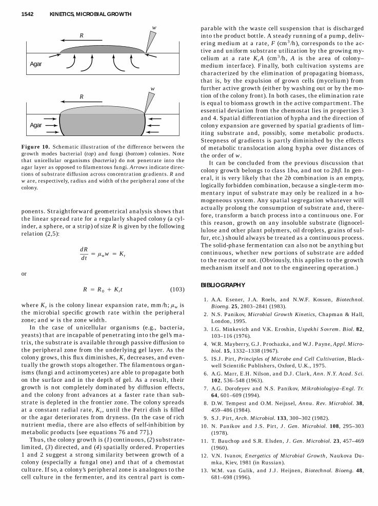
1542 KINETICS, MICROBIAL GROWTH
Agar
Agar
w
Rw
R
Figure 10. Schematic illustration of the difference between thegrowth modes bacterial (top) and fungi (bottom) colonies. Notethat unicellular organisms (bacteria) do not penetrate into theagar layer as opposed to filamentous fungi. Arrows indicate direc-tions of substrate diffusion across concentration gradients. R andw are, respectively, radius and width of the peripheral zone of thecolony.
ponents. Straightforward geometrical analysis shows thatthe linear spread rate for a regularly shaped colony (a cyl-inder, a sphere, or a strip) of size R is given by the followingrelation (2,5):
dR� l w � Kw rdt
or
R � R � K t (103)0 r
where Kr is the colony linear expansion rate, mm/h; lw isthe microbial specific growth rate within the peripheralzone; and w is the zone width.
In the case of unicellular organisms (e.g., bacteria,yeasts) that are incapable of penetrating into the gel’s ma-trix, the substrate is available through passive diffusion tothe peripheral zone from the underlying gel layer. As thecolony grows, this flux diminishes, Kr decreases, and even-tually the growth stops altogether. The filamentous organ-isms (fungi and actinomycetes) are able to propagate bothon the surface and in the depth of gel. As a result, theirgrowth is not completely dominated by diffusion effects,and the colony front advances at a faster rate than sub-strate is depleted in the frontier zone. The colony spreadsat a constant radial rate, Kr, until the Petri dish is filledor the agar deteriorates from dryness. (In the case of richnutrient media, there are also effects of self-inhibition bymetabolic products [see equations 76 and 77].)
Thus, the colony growth is (1) continuous, (2) substrate-limited, (3) directed, and (4) spatially ordered. Properties1 and 2 suggest a strong similarity between growth of acolony (especially a fungal one) and that of a chemostatculture. If so, a colony’s peripheral zone is analogous to thecell culture in the fermenter, and its central part is com-
parable with the waste cell suspension that is dischargedinto the product bottle. A steady running of a pump, deliv-ering medium at a rate, F (cm3/h), corresponds to the ac-tive and uniform substrate utilization by the growing my-celium at a rate KrA (cm3/h, A is the area of colony–medium interface). Finally, both cultivation systems arecharacterized by the elimination of propagating biomass,that is, by the expulsion of grown cells (mycelium) fromfurther active growth (either by washing out or by the mo-tion of the colony front). In both cases, the elimination rateis equal to biomass growth in the active compartment. Theessential deviation from the chemostat lies in properties 3and 4. Spatial differentiation of hypha and the direction ofcolony expansion are governed by spatial gradients of lim-iting substrate and, possibly, some metabolic products.Steepness of gradients is partly diminished by the effectsof metabolic translocation along hypha over distances ofthe order of w.
It can be concluded from the previous discussion thatcolony growth belongs to class 1b�, and not to 2bb. In gen-eral, it is very likely that the 2b combination is an empty,logically forbidden combination, because a single-term mo-mentary input of substrate may only be realized in a ho-mogeneous system. Any spatial segregation whatever willactually prolong the consumption of substrate and, there-fore, transform a batch process into a continuous one. Forthis reason, growth on any insoluble substrate (lignocel-lulose and other plant polymers, oil droplets, grains of sul-fur, etc.) should always be treated as a continuous process.The solid-phase fermentation can also not be anything butcontinuous, whether new portions of substrate are addedto the reactor or not. (Obviously, this applies to the growthmechanism itself and not to the engineering operation.)
BIBLIOGRAPHY
1. A.A. Esener, J.A. Roels, and N.W.F. Kossen, Biotechnol.Bioeng. 25, 2803–2841 (1983).
2. N.S. Panikov, Microbial Growth Kinetics, Chapman & Hall,London, 1995.
3. I.G. Minkevich and V.K. Eroshin, Uspekhi Sovrem. Biol. 82,103–116 (1976).
4. W.R. Mayberry, G.J. Prochazka, and W.J. Payne, Appl. Micro-biol. 15, 1332–1338 (1967).
5. IS.J. Pirt, Principles of Microbe and Cell Cultivation, Black-well Scientific Publishers, Oxford, U.K., 1975.
6. A.G. Marr, E.H. Nilson, and D.J. Clark, Ann. N.Y. Acad. Sci.102, 536–548 (1963).
7. A.G. Dorofeyev and N.S. Panikov, Mikrobiologiya–Engl. Tr.64, 601–609 (1994).
8. D.W. Tempest and O.M. Neijssel, Annu. Rev. Microbiol. 38,459–486 (1984).
9. S.J. Pirt, Arch. Microbiol. 133, 300–302 (1982).10. N. Panikov and J.S. Pirt, J. Gen. Microbiol. 108, 295–303
(1978).11. T. Bauchop and S.R. Elsden, J. Gen. Microbiol. 23, 457–469
(1960).12. V.N. Ivanov, Energetics of Microbial Growth, Naukova Du-
mka, Kiev, 1981 (in Russian).13. W.M. van Gulik, and J.J. Heijnen, Biotechnol. Bioeng. 48,
681–698 (1996).

KINETICS, MICROBIAL GROWTH 1543
14. N.S. Pechurkin, Populational Microbiology, Novosibirsk,Nauka 1978, p. 277.
15. R.E. Buchanan, J. Infect. Dis. 23, 109–125 (1918).16. G. Stephanopoulos, and J.J. Vallino, Science 252, 1675–1680
(1991).17. Y. Kashiwaya, K. Sato, N. Tsuchiya, S. Thomas, D.A. Fell, R.L.
Veech, and J.V. Passonneau, J. Biol. Chem. 269, 25502–25514(1994).
18. J.J. Vallino, and G. Stephanopoulos, Biotechnol. Bioeng. 41,633–646 (1993).
19. A. Marx, A.A. de Graaf, W. Wiechert, L. Eggeling, and H.Sahm, Biotechnol. Bioeng. 49, 111–119 (1996).
20. A. Cornish-Bowden, Principles of Enzyme Kinetics. Butter-worths, London-Boston, 1976.
21. N. Michaelis and M.I. Menten, Biochem. Z. 49, 333–369(1913).
22. G.E. Briggs and J.B.S. Haldane, Biochem. J. 19, 338–339(1925).
23. H. Gutfreund, Discuss. Faraday Soc. 20, 167–173 (1955).24. J.B.S. Haldane, Enzymes. Longmans Green, London, 1930.25. J. Monod, J. Wyman, and J. Changeux, J. Mol. Biol. 12, 88–
118 (1965).26. C.H. Wang and A.L. Koch, Bacteriol. 136, 969–975 (1978).27. O. Rahn, Physiology of Bacteria, P. Blackiston’s, Philadelphia,
1932.28. P.F. Verhulst, Correspondence Mathematique et Physique
10(1), 113–121 (1838).29. J. Monod, Recherches sur la Croissance des Cultures Bacter-
iennes, Paris, Hermann and Co, 1942.30. J. Monod, Ann. Inst. Pasteur 79, 390–410 (1950).31. F.F. Blackman, Ann. Bot.–London 19, 281–293 (1905).32. S.D. Varfolomeyev, in S.D. Varfolomeyev ed., Modern Prob-
lems of Biokinetics, Moscow University Publishers, Moscow,1987, pp. 6–77.
33. J. Monod, Ann. Rev. Microbiol. 3, 371–394 (1949).34. N.D. Jerusalimsky, in E.O. Powell, C.G.T. Evans, R.E.
Strange, and D.W. Tempest eds., Continuous Cultivation ofMicroorganisms, H.M. Stationery Office, Salisbury, U.K.,1967, pp. 23–33.
35. I.A. Shvytov, Zhurnal Obshchei Biologii 35, 904–910 (1974).36. J.M. Romanovsky, N.V. Stepanova, and D.S. Chemavski,
Mathematical Biophysics, Moscow, Nauka, 1984.37. T.E. Shehata and A.G. Marr, J. Bacteriol. 107, 210–216
(1971).38. A.F. Guady Jr., A. Obayashi, and E.T. Gaudy, Appl. Microbiol.
22, 1041–1047 (1971).39. D.K. Button, Microbiol. Rev. 49, 270–297 (1985).40. B.R. Robertson and D.K. Button, Bacteriology 138, 884–895
(1979).41. G. Teissier, Ann. Physiol. Physicochem. Biol. 12, 527–586
(1956).42. D.E. Contois, J. Gen. Microbiol. 21, 40–49 (1959).43. H. Moser, Carnegie Inst. Wash. Pub. 614 (1958).44. E.O. Powell, in E.O. Powell, C.G.T. Evans, R.E. Strange, and
D.W. Tempest eds., Continuous Cultivation of Microorgan-isms, H.M. Stationery Office, Salisbury, U.K., 1967, pp. 34–55.
45. J.F. Andrews, Biotechnol. Bioeng. 10, 707–723 (1968).46. U. Pawlowsky, S.A. Howell, and C.T. Chi, Biotechnol. Bioeng.
15, 905–916 (1973).47. A. Campbell, Bacteriol. Rev. 21, 263–272 (1957).48. C.L. Cooney, Ann. N.Y. Acad. Sci. 326, 295–314 (1979).49. E.O. Powell, C.G.T. Evans, R.E. Strange, and D.W. Tempest
eds., Continuous Cultivation of Microorganisms, H.M. Sta-tionery Office, Salisbury, U.K., 1967, pp. 259–261.
50. D. Ramkrishna, A.G. Fredrickson, and H.M. Tsuchiya, Bio-tech. Bioeng. 9, 129–170 (1967).
51. M.M. Domach, S.K. Leung, R.E. Cahn, G.G. Cacks, and M.L.Shuler, Biotech. Bioeng., 26, 203–216 (1984).
52. J.W. Jeong, J. Snay, and M.M. Ataai, Biotechnol. Bioeng. 35,160–184 (1990).
53. I. Malek, in I. Malek ed., Continuous Cultivation of Microor-ganisms: A symposium, Publishing House of Czech. Acad. Sci.,1958, pp. 11–28.
54. D. Herbert, Symp. Soc. Gen. Microbiol. 11, 391–416 (1961).55. P. Agrawal, H.C. Lim, and D. Ramkrishna, J. Chem. Tech.
Biotechnol. 33B, 155–163 (1983).56. D.S. Kompala, D. Ramkrishna, N.B. Jansen, and G.T. Tsao,
Biotechnol. Bioeng. 28, 1044–1055 (1986).57. B.G. Turner, D. Ramkrishna, N.B. Jansen, Biotechnol. Bioeng.
34, 252–261 (1989).58. D.W. Tempest, J.R. Hunter, and J. Sykes, J. Gen. Microbiol.
39, 355–366 (1965).59. D.W. Tempest, D. Herbert, and P.J. Phipps, in E.O. Powell,
C.G.T. Evans, R.E. Strange, and D.W. Tempest eds., Contin-uous Cultivation of Microorganisms, H.M. Stationery OfficeSalisbury, U.K., 1967, pp. 240–253.
60. A.T. Henrici, Morphologic Variation and the Rate of Growthof Bacteria, Charles C. Thomas, Springfield, Ill., 1928, p. 194.
61. A.L. Koch, Crit. Rev. Microbiol. 19, 17–42 (1973).62. S. Wold, K. Skarstad, H.B. Steen, T. Stokke, E. Boye, EMBO
J. 13, 2097–2102 (1994).63. C.E. Helmstetter, S. Cooper, O. Pierucci, and E. Revela, Cold
Springs Harb. Symp. Quant. Biol. 33, 809–822 (1968).64. S. Cooper, Res. Microbiol. 141, 17–29 (1990).65. A.L. Koch, J. Gen. Microbiol. 45, 409–417 (1966).66. J.F. Collins, and M.H. Richmond, J. Gen. Microbiol. 28, 15–
33 (1962).67. A. Novick, in G. Tunevall ed., Recent Progress in Microbiology,
Blackwell Scientific Publications, Oxford, U.K., 1959, pp. 403–415.
68. J. Adams, T. Kinney, S. Thompson, L. Rubin, and R.B. Helling,Genetics 91, 627–637 (1979).
69. R. Freter, R.R. Freter, and H. Brickner, Infect. Immunol. 39,60–84 (1983).
70. I.G. Minkevich, A.Y. Krynitskaya, and V.K. Eroshin, Mikro-biologiya (Engl. Tr.) 56, 254–258 (1987).
71. W.R. Chesbro, T. Evans, and R. Eifert, J. Bacteriol. 139, 625–638 (1979).
72. B.C. Goodwin, Eur. J. Biochem. 10, 511–514 (1969).73. P.S.S. Dawson, Can. J. Microbiol. 11, 893–903 (1965).
See also MICROBIAL GROWTH MEASUREMENT, METHODS.
Related Documents