Churn Prediction Modelling in Mobile Telecommunications ...

CHURN PREDICTION MODELLING IN MOBILE

TELECOMMUNICATIONS INDUSTRY: A CASE STUDY

OF SAFARICOM LTD

BY

KAIRANGA JAMES MACHARIA

SCHOOL OF MATHEMATICS

COLLEGE OF BIOLOGICAL AND PHYSICAL SCIENCE

UNIVERSITY OF NAIROBI

A project submitted in partial fulfilment of the requirement for the degree of Master of

Science in Social Statistics

JULY 2012

DECLARATION

Candidate:

This project report is my original work and has not been presented for a degree in any other

university.

li£ iLKairanga James Macharia 156/64577/2010

Supervisor:

This project report has been submitted for examination with my approval as university supervisor

Signature

Dr. Kipchirchir Isaac Chumba

n.„ W

I

ACKNOWLEDGEMENT

I take the first opportunity to thank God for gift of life and good health. Secondly, offer my

sincerest gratitude to my supervisor, Dr. Kipchirchir Isaac Chumba, who has supported me

throughout my project with his patience and knowledge whilst allowing me the room to work with

freedom of thought. One simply could not wish for a better or friendlier supervisor. I acknowledge

my lectures: Prof. Manene Moses M., Prof. Otieno Joseph A. M., Mr. Ndiritu John. M. and Mrs.

Wang'ombe Anne W. for the knowledge they have impacted me throughout my course work. Last

but not least Consumer Planning and Pricing section within Safaricom for providing me with the

required data for analysis.

n

DEDICATION

I dedicate the project to my lovely wife Winnie and daughter Tiffany.

iii

ABSTRACT

The focus of telecommunication companies has shifted from building a large customer base into

keeping customers in house. For these reasons, it is valuable to know which customers are likely to

switch to a competitor through porting out or purchasing a competitor line.

Since acquiring new customers is more expensive than retaining existing customers, chum

prevention can be regarded as a popular way of reducing the company's costs. In this study, Cox

proportional hazard model and decision tree model are compared with conventional model.

The first model, the Cox model, is based on the theory of survival analysis, whereas the second

model, a decision tree, is commonly used in data mining. Both models are tested on a selection of

pre-paid customers from the database provided by Safaricom Limited.

Current conventional prediction used by Safaricom Limited was improved significantly by using

Cox proportional hazard and decision tree as they both performed better on the ROC curve.

However, for the duration under consideration decision tree performed better than Cox proportional

model.

Decision tree model selected gave probability of chum which is an improvement from conventional

model that only gives binary results of chum and not chum. Also, where the decision tree yields

approximately 50 percent probability of chum conventional model gave varying churn status.

IV

LIST OF ABREVIATIONS

AON - Age On Network

ARPU - Average Revenue per User

DMTV - Direct Mail Television

CART - Classification and Regression Trees

CCK - Communications Commission of Kenya

c.d.f - cumulative distribution function

CDR - Call Detail Record

CHAID - Chi Square Automatic Interaction Detection

CLV - Customer Lifetime Value

CRM - Customer Relationship Management

CVM - Customer Value Management

EDA - Exploratory Data Analysis

EDF - Empirical Distribution Function

EDGE - Enhanced Data Rates for GSM Evolution

ETACS - Extended Total Access Communications System

FPR - False Positive Rate

GA - Genetic Algorithm

Global Systems for Mobile - GSM

Gok - Government of Kenya

K.PTC - Kenya Posts and Telecommunications Corporation

MS1SDN - Mobile Number

OTA - Over The Air

PABX - Private Automatic Branch Exchange

PDN - Packetstream Data Networks

v

p.d.f - probability density function

Pic - Public limited company

RFM - Recency Frequency Monetary

ROC - Receiver Operating Characteristic

SIM - Subscriber Identity Module

SMS - Short Messaging Service

TKL - Telkom Kenya Limited

TPR - True Positive Rate

USSD - Unstructured Supplementary Service Data

vi

TABLE OF CONTENTS

DECLARATION I

ACKNOWLEDGEMENT II

DEDICATION III

ABSTRACT IV

LIST OF ABREVIATIONS V

TABLE OF CONTENTS VII

LIST OF TABLES IX

LIST OF FIGURES X

CHAPTER 1: INTRODUCTION 1

1.1 Background............................................................................................................................... 1

1.2 Problem Statement................................................................................................................. 8

1.3 Research Question...................................................................................................................9

1.4 Objectives...................................................................................................................................9

1.5 Significance of the study .................................................................................................... 10

CHAPTER 2: LITERATURE REVIEW 12

CHAPTER 3: METHODOLOGY 20

3.1 Introduction........................................................................................................................... 20

3.2 Data M ining............................................................................................................................ 21

3.3 Cox Proportional Hazard Mo d el .....................................................................................25

3.4 Decision Tree Model............................................................................................................. 30

3.5 Population and Study Sample.............................................................................................32

vii

3.6 Test statistics for Model Comparison.............................................................................33

3.6.1 ROC Curve................................................................................................................................33

3.6.2 Kolmogorov-S mirnov Test (K-S Test) .............................................................................35

3.6.3 Gini Coefficient...................................................................................................................... 37

3.7 Modelling Process.................................................................................................................39

CHAPTER 4: DATA ANALYSIS AND RESULTS 46

4.1 Exploratory Data Analysis..............................................................................................46

4.2 Variable Reduction...............................................................................................................50

4.3 Model Estimation................................................................................................................... 52

4.4.1 Decision Tree ......................................................................................................................... 54

4.4.2 COX PROPORTIONAL HAZARD MODEL....................................................................................... 55

4.4 Model Validation.................................................................................................................. 56

CHAPTER 5: CONCLUSIONS AND RECOMMENDATIONS 61

5.1 Conclusions............................................................................................................................ 61

5.2 Recommendations...................................................................................................................61

APPENDICES 63

Appendix 1: Fit Statistics Table .................................................................................................... 63

Appendix 2: Tree Leaf Report..........................................................................................................65

REFERENCES 65

viii

LIST OF TABLES

Table 4.1 Sample statistics variables minimum, mean and maximum values 47

Table 4.2 Sample variables per subscriber 48

Table 4.3 Chum status 51

Table 4.4 Variables Summary 52

Table 4.5 Partition Summary 52

Table 4.6 Summary statistics for class targets 53

Table 4.7 Important variables picked by the decision tree 54

Table 4.8 Summary of Censored Events 55

Table 4.9 Analysis of Maximum Likelihood Estimates (MLE) 56

Table 4.10 Statistics Results from the fitted Models 58

Table 4.11 Comparison of Decision Tree Model and Conventional Model 59

IX

LIST OF FIGURES

Figure 3.1 ROC Curve 33

Figure 4.1 Exploration of AON distribution 49

Figure 4.2 Exploration of age distribution 49

Figure 4.3 Chum Status 51

Figure 4.4 Comparing train and validate data set 57

Figure 4.5 Comparing train and validate data set using ROC 57

x

CHAPTER 1: INTRODUCTION

1.1 Background

Chum is a measure of subscriber attrition from a given mobile operator network, and is defined as

the number of subscribers who discontinue using a particular network during a specified time period

divided by the average total number of customers or employees over that same time period.

In a dynamic business, chum rate indicate subscriber response to tariff, promotions, competitor

network activities etc. As such, chum rate is an important business metric. To estimate future chum

rates predictive chum modelling is applied.

Largest mobile operators such as Vodafone have long appreciated that the cost of acquiring a new

customer is incrementally greater than the cost of retaining an existing one. Thus, chum data,

alongside subscriber acquisition costs, has become a key measure used by industry analysts and

financial commentators to determine mobile operator performance.

Safaricom, which started as a department of Kenya Posts and Telecommunications Corporation

(KPTC), the former monopoly operator, launched operations in 1993 based on an analogue

Extended Total Access Communications System (ETACS) network which was upgraded to Global

Systems for Mobile (GSM) in 1996 (license awarded in 1999). Safaricom was incorporated on

April 1997 as a private limited liability company.

In accordance with the Government o f Kenya’s policy of divesting its ownership in public

enterprises, the Government of Kenya through the Treasury Department, on 28th March 2008 made

1

available to the public 10 billion of the existing ordinary shares of par value ksh. 0.05 each, of the

Company. This represents 25 percent of the total issued share capital of Safaricom from the

Government of Kenya's shareholding in Safaricom Limited.

As at 31st March 2009, the company had 6.175 million registered users, a customer base of 13.36

million, 8,650 retail outlets countrywide, 51 paybill partners, 301 3G enabled base stations in

Nairobi, Mombasa, Naivasha and Eldoret.

In 2009, Safaricom won awards for Best Mobile Money Service in the GSMA. In Global Mobile

Awards it was the winner in the Best Broadcast Commercial Category for its entry of the M-PESA

Send Money Home', in the UN World Business and Development Award it was among the 10

private companies recognized globally for their contribution to the achievement of millennium

development goals through M-PESA, in the Kenyan Banking Awards it was the winner in the

product innovation category (M-PESA) and in the Stockholm Challenge, the winner in the

Economic Development Category ( M-PESA).

M-PESA is a Safaricom product that allows users to transfer money using a mobile phone. Kenya is

the first country in the world to use this service, which is offered in partnership between Safaricom

and Vodafone. M-PESA is available to all members of the public, even if they do not have a bank

account or a bankcard.

Safaricom offers mobile voice services using GSM-900 and GSM-1800 technologies. It launched

GPRS services in July 2004 and Enhanced Data Rates for GSM Evolution (EDGE) services in June

2006. In 2007 it was formally granted Kenya's first license to operate a 3G network.

2

Safaricom business model focuses on pre-paid customers (pay-in-advance) without long-term

contract commitments. It requires most o f its customers to pay for services in advance to limit the

customer-related credit risk.

It focuses on:

I. Low-income clients to boost the customer base.

II. Expansion of its GSM coverage footprint in rural areas and capacity levels in key urban

areas.

III. Improve the performance and reliability of its services.

IV. Introducing new and innovative products.

Safaricom offers all and post-paid users a variety of value priced service plan options and products.

Safaricom has aligned itself with other business partners including distributors, suppliers and

technology partners. These arrangements help Safaricom maintain a low cost structure while

ensuring high quality customer products and services. The company bundles its products and

services with products of globally established companies with the goal of deploying reliable, high-

quality cellular products and services to the mass market and competing effectively with other

mobile providers.

In this regard, Safaricom has a working relationship with Vodafone Group Pic, an established leader

in global mobile telecommunications industry. The amount of investment Vodafone has made is

among the largest ever made by any foreign company in Kenya. Vodafone also provides Safaricom

with the opportunity to be a member of its global procurement group and to benefit from

Vodafone's experience in other countries strong marketing efforts, rapid product deployment and

maintaining and growing strong brand recognition.

3

The company has focused on enhancing its image by involving itself in the community and

focusing on local themes, which may resonate with the targeted customer base.

During 2008, Safaricom formulated an aggressive growth campaign to increase its subscriber base-

by launching a series of promotions, investing heavily in subscriber acquisition and increased the

core network capacity by targeting rural areas.

By virtue o f the 60 percent shareholding held by the Government of Kenya (GoK), Safaricom was a

state corporation within the meaning of the State Corporations Act (Chapter 446) Laws of Kenya,

which defines a state corporation to include a company incorporated under the Companies Act

which is owned or controlled by the Government or a state corporation. Until 20 December 2007,

the GoK shares were held by Telkom Kenya Limited (TKL), which was a state corporation under

the Act.

Follow ing the offer and sale of 25 percent of the issued shares in Safaricom held by the GoK to the

public in March 2008, the GoK ceased to have a controlling interest in Safaricom under the State

Corporations Act and therefore the provisions of the State Corporations Act no longer apply to it.

To attract new investments into the ICT sector, the regulation capping foreign ownership of

telecoms companies at 80 percent was relaxed to allow foreigners to launch operations without a

local partner.

The introduction of new players and a changing regulatory landscape brought new challenges to

Safaricom and the industry as a whole. A more competitive industry landscape placed downward

pressure on Safaricom market share of gross additions in the medium term. As retail tariffs reduced,

4

ARPU reduced for both prepay and post pay subscribers for the industry as a whole. Enhanced

competition created the need for the company to maintain higher levels of selling and limit general

and administrative expense levels. This was due to the potential requirement for higher advertising

costs to protect the subscriber base and increased payroll costs to retain key managerial talent. It led

to focus on product development. In 2009 Safaricom launched Kenya's first mobile internet portal

(www.safaricom.com) to provide free content for its over 1.6 million subscribers who access the

Internet using their phones. The portal enabled Safaricom subscribers to access both local and

international content direct from their mobile phones.

Safaricom then launched Africa's first fully solar-powered phone, branded Simu ya Solar. The new

solar-powered mobile phone went on sale in Kenya in August 2009 at ksh. 499. The solar-powered

phone was produced by the Chinese ZTE Corporation.

Safaricom announced in August 2009 that it has bought 100 percent of a second local WiMAX

operator, Packetstream Data Networks (PDN) and signed an agreement with Nokia and DMTV to

introduce mobile TV service.

In mid-May 2009, Safaricom joined the race to capture the data market in the telecoms industry and

launched the caller ring back tune service. The service branded Skiza, enabled subscribers to choose

a preferred song and set it as their ring back tune. Other products launched in subsequent years

included:

I. tXt-ten for ten (group SMS) - A mobile chat service that enabled subscribers to quickly send

the same message to several members of a group.

II. Advantage Contracts - Offers subscribers an opportunity to control their call costs.

5

III. Advantage Plus - Enabled corporate customers to give their staff a limit on their monthly

expenditure.

IV. Safaricom Mail - Email service in conjunction with Google.

V. Toll Free Services - Where called party pays for calls to a toll-free number.

VI. Corporate Direct Connectivity - Direct connection between the customer's PABX and

Safaricom's network facilitates voice communication.

VII. Winback SMS for Roaming - Allows Safaricom to Win-Back visitors lost to a competitor's

network

VIII. Automatic Device Configuration - Subscribers could request for data and network settings

automatically via USSD and SMS and have these delivered directly to their handsets over

the air.

IX. OTA SIM Swap - Allows Safaricom pre-paid subscribers who have lost their SIM Cards to

do a SIM Swap on their handsets.

X. Express Auto bar - A quick one-stop service for all individual customers and guarantees

active post-paid lines.

XI. Kama Kawaida with Rwanda - Here, Safaricom teamed with MTN Rwanda to offer

subscribers seamless service availability at their home tariffs when travelling across the two

countries.

Price wars began in August 2010 when Zain Kenya slashed its on-net prices by 80 percent. Yu and

Orange network followed immediately by reducing calling rates even further. Safaricom countered

by introducing Masaa Tariff which reduced calling rates to ksh. 3. It soon became clear that

strategy will not be to acquire new customers since competitor networks are charging low rates but

managing current subscriber base.

6

This lead to the launch of loyalty scheme “ Bonga" to manage subscribers by offering reward on the

number of points accumulated through calling, data and SMS. Subscribers were able to accumulate

points and redeem free minutes and sms. This was later improved to accommodate redemption of

handsets, modem and laptops.

.In a nutshell, below is the life cycle of a Safaricom subscriber:

I. Active - This is the duration of the validity of the recharged voucher topped up. In this state,

the subscriber can make or receive calls and sms browse the internet using a data enabled

handset and transact MPESA.

II. Expiry - this is the next state after subscriber enters after active state if they do not top-up

before expiry of the validity period of the card that they previously topped up. Here, the

subscriber can only receive but cannot make chargeable calls and sms. When a subscriber

tops up they go back to active state. Expiry state last 30 days after which subscriber enters

pooled state.

III. Pool - Here, the subscriber cannot make or receive calls or access any Safaricom service.

It's the initial process of churn and it last for 120 days. In this state, a subscriber cannot top-

up as was the case in expiry state to return to active state.

IV. Inactive - This is the final stage of chum where the line is recycled and resold in the market.

Here the subscriber loses the line together with all resources accumulated by the line such as

Bonga points, airtime balance, data bundles and MPESA monies not withdrawn.

The costs of acquisition of a subscriber are made up of:

I. SIM card cost

II- CCK licence cost

III. Network cost

7

IV. Dealer costs

V. Administration costs.

VI. Set-up costs.

These costs are accrued before a subscriber becomes active on our network. Considering there are

also costs to maintain subscriber on the network, it takes on average more than 6 months to recoup

acquisition cost for a new subscriber.

From quarterly sector statistics report by CCK, 2nd Quarter October-December 2011/2012, total

net additions by all mobile operators in December 2011 were 1.5 million. Net addition is the

increase in the total subscriber count from the start of the period to the end of the period. This

implies that all mobile operators in Kenya cannot rely on increasing their subscribers’ base based on

new joiners.

1.2 Problem Statement

Safaricom operates in an industry where switching costs is very low. Subscribers require ksh. 200 to

port to any network. Cost of purchase of competitor line is ksh. 50. Considering acquisition costs

which on average takes more than 6 months to recoup and reducing numbers subscribers available

for new connection, customer churn is the focal concern.

To manage chum, Safaricom has adopted Customer Value Management (CVM), where efforts are

being put in place to ensure no chum for upper and middle segment of subscribers and only selected

chum is to be allowed for lower segment of the subscribers.

8

However, due to the nature of pre-paid mobile telephony market which is not contract-based,

subscriber chum is not easily traceable or definable, thus the need to improve on the conventional

model.

1.3 Research Question

The research question is stated as follows:

Is it possible to improve on current conventional methods of predicting chum?

In order to address this question, the following two sub questions are formulated:

I. How well do survival and decision tree model perform in comparison to the conventional

models?

II. Do the two models have an added value compared to the conventional models?

1.4 Objectives

The broad objective is to find out the most accurate chum prediction model by comparing Cox

proportional hazard model and decision tree model against conventional model so as to accurately

determine of probability of each subscriber churning.

Specific objectives:

1. To formulate a chum model using Cox proportional hazard and decision tree models.

2. To compare results of models formulated to current conventional models and determine

the best model.

9

3. To determine the probability o f churning for every subscriber based on the best model

selected.

1.5 Significance of the study

Current conventional method focus on reduction in ARPU, which is affected by many other

variables such as:

I. Competitor activities.

II. Demographic factors.

III. Usage factors.

IV. Economic factors.

V. Social factors.

< 4 *

Cox proportional model incorporates all this variables as well as time to chum thus can provide

more accurate prediction of chum for individual subscribers. Decision tree is simple to understand

and offers ability to do oversampling for chum which it considers as unlikely an event.

The model will be important indicator of the success of pricing and promotion strategies adopted by

the company. Currently, the focus of pricing of products and services is purely based on profits

which are not customer centric. Customers who have for many years made significant contribution

to revenue are moving to competitor network because the company seems not to value their loyalty.

Chum probability created will be the input of Customer Lifetime Value (CLV) models to be

developed that seek to provide a useful way to apportion value to a subscriber (or subscriber group)

based on cumulative cash flow from a subscriber relationship and the benefits of loyalty and

10

advocacy that increase over time. CLV will provide strategic teams with a means to gauge the

effectiveness of their acquisition costs and retention strategies.

11

CHAPTER 2: LITERATURE REVIEW

There is a significant relationship between customer loyalty, satisfaction, trust and switching costs

in mobile telephony market. In this fiercely competitive arena, subscribers demand tailored

products and better sendee at lower prices, while service providers focus on customer acquisition as

their primary focus.

Yankee (2001) indicated that mobile operators estimate the cost of acquiring new subscribers at

seven times more than the annual cost of retaining an existing subscriber on an average basis. The

emergence of the digital economy has intensified the problem of churn management Lejeune (2001)

stated that a company’s initiatives to handle churn and profitability issues have been directed to more

customer-oriented strategies. A customer relationship management (CRM) framework based on the

integration of the electronic channel would incorporate the electronic dimension and be enhanced

by the development of adequate tools for the collection, treatment and analysis of data which plays

a central role in chum management.

Chum amplitude is negatively correlated with the efficiency of data-mining tools, and the

relationship between chum and CRM tools is linear. An analytical framework based upon

sensitivity analysis could anticipate the possible impact induced by the ongoing data-mining

enhancements on chum management and the decision-making process

According to Olafsson et al. (2008), there are two different types of chum namely:

I. Voluntary chum - Which means that established customers choose to stop being customers.

II. Forced chum - Which refers to those established customers who no longer are good

customers and the company cancels the relationship.

12

Burez et al. (2008) divided the voluntary chumers to two groups:

I. Commercial chumers - Subscribers who do not renew their fixed term contract at the end of

that contract.

II. Financial chumers - Subscribers who stop paying during their contract to which they are

legally bound.

Seo et al. (2008) investigated retention factors in telecommunications industry by examining other

features and variables. Aim was to examine:

I. How factors that affect switching costs and customer satisfaction, such as length of

association, service plan complexity, handset sophistication and the quality of connectivity,

drive customer retention behavior.

II. How customer demographics such as age and gender affect their choice of service plan

complexity and handset sophistication, leading to differences in customer retention behavior.

They used binary logistic regression model and a two-level hierarchical linear model. The factors

analysed consisted o f complexity of service plan, handsets sophistication, length of association and

connectivity. Customer demographics to be related to these factors are gender and age.

The results showed that:

I. The more complex service plan, more sophisticated handset, longer customer association,

higher connectivity quality of wireless is positively related to customer retention behaviour.

II. Different age and gender groups revealed differences in wireless connectivity quality and

service plan complexity affecting their customer retention behaviour

HI. They did not experience differences in terms of length of customer association and handset

sophistication.

13

The results generated questions on why different age and gender groups would differ on the

connectivity quality of wireless service and not on handset sophistication.

Yan et al. (2005) constructed a predictive chum model for pre-paid customer segment. Due to the

limited availability of data, they exploited Call Detail Record (CDR). To construct their predictive

model, they extracted the calling links, that is, who called whom as inputs to neural network model

Using the CDR, they defined two categories of calling links as follows:

I. Direct calling neighbour - A person who calls the customer or whom the customer calls.

II. Indirect calling neighbour - A person who calls the same numbers as the customer does.

Utilizing these neighbours, they discovered the calling community of each customer and

hypothesized that people from a calling community behave in a similar way. So, they supposed that

if a customer most frequently called parties churned from the same service provider, the customer

may also eventually chum.

With the intention of building the chum predictive model they used the CDR data of July and

August to predict the chum in December. In addition, they were provided with chum labels that

showed w ho churned, in both November and December. Their research task was to develop a chum

prediction model, with chum in December as the dependent variable (Prediction Target) and with

independent variables being the CDR data in July and August and the chum information in

November. They analysed the data by using decision tree and neural networks. For the neural

network, if the customer service representatives contact the 10 percent of customers with the

highest scores from the model, they are able to correctly identify 20 percent of the chumers.

14

They found that the neural networks outperform the decision tree, which performs even worse than

random sampling for a higher contact rate.

Jahromi (2009) developed a dual-step model building approach, which consisted of clustering phase

and classification phase. The customer base was divided into four clusters, based on their Recency

Frequency Monetary (RFM) related features, with the aim of extracting a logical definition of

chum, and secondly, based on the chum definitions that were extracted in the first step.

In the model building phase, the decision tree (CART algorithm) was utilized to build the predictive

model with the aim of comparing the performance of different algorithms. Neural networks

algorithm and different algorithms of decision tree were utilized to construct the predictive models

for chum in the developed clusters. Evaluating and comparing the performance of the employed

algorithms based on “gain measure".

Jahromi concluded that employing a multi-algorithm approach in which different algorithms are

used for different clusters, yields the maximum “gain" among the tested algorithms.

Furthermore, to deal with imbalanced dataset, a cost- sensitive test was carried out using learning

method as a remedy for handling the class imbalance. This revealed that both simple and cost-

sensitive predictive models have a considerable higher performance than random sampling in both

CART model and multi-algorithm model. Additionally, cost-sensitive learning was proved to

outperform the simple model only in CART model but not in the multi-algorithm.

According to Jahromi, the problem that telecommunication companies face is to recognize the

subscribers with high probability of chum in close future so as to target them with incentives in

15

order to convince them to stay. However, due to the absence of an accurate model for monitoring

their clients* behaviour, telecommunication companies are unable to distinguish the chumers from

non-chumers. In such instances they have two options:

I. Send all customers the incentives, which was clearly a waste of money.

II. Quit the chum management program and focus on acquisition program which is

considerably more costly than the retention approach.

According to Jahromi, not only did the model helped in distinguishing the real chumers, but also, it

prevented the waste of money attributed to the mass marketing.

Owczarczuk (2009) studied chum models for customers in the cellular telecommunication industry

using large data marts and tested the usefulness of the popular data mining models to predict chum

of the clients of the Polish cellular telecommunication company. The study was conducted on

subscribers who are:

I. More likely to chum.

II. Less stable.

III. Little is known about them.

Owczarczuk utilised all subscriber usage variables and tested the stability of models across time for

all the percentiles of the lift curve. Test sample were collected six months after the estimation of the

model.

Logistic regression, linear regression, Fisher linear discriminant analysis and decision trees models

were used. The basis of choice of the model was the need to use interpretable models which gives

understanding of the reasons (or at least a symptom) of chum. Owczarczuk claimed that linear

models like regression or Fisher discriminant analysis have a simple interpretation. For example,

16

positive coefficient by a variable suggests higher likelihood of chum. Decision trees too have a

clear interpretation which can be expressed in terms of what-if rules.

Data set consisted of the train, calibration and test datasets. Data in the train sample and the

calibration sample came from the dataset collected at the same time, which was then split randomly

into the train and validation part. The test sample was collected six months after the train and

calibration sample.

The models were tested using lift curves that measured the relation of chumers in the top quartiles

of the score generated by the models to the fraction of chumers in the whole population (lifts

expressed as factors not as percentage) since all the linear models had similar performance

regardless of the additional variable selection method (stepwise, backward, forward, none). The

logistic regression was slightly better than linear regression and Fisher discriminant analysis.

Applying preliminary variable selection to decision trees gave similar results to the full decision

tree, so they present only decision trees with the preliminary variable selection.

Main findings were that linear models are more stable than decision trees that get old quickly and

their performance weakens in time, especially in top quartiles of the score. Nevertheless, the study

showed that pre-paid chum can be effectively predicted using large data mart. It was suggested that

as far as future work is concerned, it would be interesting to model chum in the sector that is

somewhere between post-paid and pre-paid - the mix sector. Mix clients have to sign contract and

personal data is available for them, like for the post-paid customers. In addition, they make recharge

which makes them similar to prepaid.

17

Ahn et al. (2006) conducted an exploratory research in which they aimed at finding the most

influential factors on customer chum. In their research, they considered a mediator factor named

"Customer's Status”, between churn determinants and customer churn in their model, and

mentioned that “Customer's Status” (from active use to non - use or suspended) change is an early

signal of total customer chum.

In the research, a mediator was taken into account between chum determinants and customer chum,

and it was hypothesized that a customer's status change is an early signal of total customer chum. In

conducting their empirical analysis, they draw a random sample of subscribers of a leading

telecommunications service provider. The account had to be active during the time period between

September 2001 and November 2001. For those customers, all accounts were tracked and examined

for eight month from September 2001 to April 2002, and ‘‘Churn" was defined as the event in which

a subscription was terminated by the end of April 2002. That is, chum happened during the period

from December 2001 to April 2002. For churners' 3-month, 2-month, and 1-month prior data was

collected before the actual termination. For the non-chumers, the most recent last 3 months of data

was collected (from February 2002 to April 2002).

From the collected data they extracted the subscriber's usage and billing data and also the

demographic data. The available data consisted of:

I. Billed amounts.

II. Accumulated loyalty points.

III. Call quality-related indicators.

IV. Handset-related information.

V. Calling plans.

VI. Gender.

18

The results showed that dissatisfaction indicators, such as number of complaints and call drop rate

have a significant impact on the probability o f chum. Besides, it was revealed that loyalty points

such as membership card programs have a significant negative impact on the probability of

customer chum.

Moreover, surprisingly the findings showed that heavy users are more likely to chum and also

customer status was found to have significant impact on the probability of chum. In addition they

found out that customer status has a significant impact on the probability of chum. Change of

customer's status from active use to either non-use or suspended increases the chum probability.

19

CHAPTER 3: METHODOLOGY

3.1 Introduction

Survival analysis is a collection of statistical methods which model time-to-event data. Central is

the occurrence of a well-defined ‘event’. The variable of interest is the time until this event occurs.

This is in contrast with approaches like regression methods and neural networks which model the

probability of an event. Depending on its application, the event of interest can be the failure of a

physical component or the time to death. In the context of data mining the event of interest is

typically the time until chum or the time until the next purchase.

There are many different types of survival models. Of concern will be survival model that

incorporate a regression component, since these regression models can be used to examine the

influence o f explanatory variables on the event time. In this context, such explanatory variables are

often called covariates. There are two commonly used classes of regression models, that is:

I. Accelerated failure time models.

II. Proportional hazard models.

Accelerated failure time models are based on a survival distribution. Common employed

distributions are Weibull, exponential and log-logistic. In accelerated failure time models, the

regression component affects survival time by rescaling the time axis. The Cox proportional hazard

model is the most popular survival regression model available. It does not make any assumptions on

the survival function as opposed to accelerated failure time models. The regression component

affects the hazard curve through multiplication. Many improvements and adjustments have been

made to the Cox model since the introduction of the model.

20

Non-parametric approach covers techniques that do not rely on data belonging to any particular

distribution. These include, among others, distribution free methods, which do not rely on

assumptions that the data are drawn from a given probability distribution. As such it is the opposite

of parametric statistics. It includes non-parametric statistical models, inference and statistical tests

and non-parametric statistics (in the sense o f a statistic over data, which is defined to be a function

of a sample that has no dependency on a parameter), whose interpretation does not depend on the

population fitting any parameterized distributions. Statistics based on the ranks of observations are

one example of such statistics and these play a central role in many non-parametric approaches.

Decision tree model of commutation which is an algorithm or communication process is considered

to be basically decision tree, that is, a sequence of branching operations based on comparisons of

some quantities, the comparisons being assigned the unit computational cost. Data mining

techniques will be used to obtain data from the enterprise warehouse the modelling purpose.

3.2 Data Mining

Data mining, or knowledge discovery, is the computer-assisted process of digging through and

analysing enormous sets of data and then extracting the meaning of the data. Data mining tools

predict behaviours and future trends, allowing businesses to make proactive, knowledge-driven

decisions. Data mining tools can answer business questions that traditionally were too time-

consuming to resolve. They scour databases for hidden patterns, finding predictive information that

experts may miss because it lies outside their expectations.

Data mining derives its name from the similarities between searching for valuable information in a

large database and mining a mountain for a vein of valuable ore. Both processes require either

21

sifting through an immense amount of material, or intelligently probing it to find where the value

resides.

Although data mining is still in its infancy, companies in a wide range of industries - including

retail, finance, health care, manufacturing transportation, and aerospace - are already using data

mining tools and techniques to take advantage of historical data. By using pattern recognition

technologies and statistical and mathematical techniques to sift through warehoused information,

data mining helps analysts recognize significant facts, relationships, trends, patterns, exceptions and

anomalies that might otherwise go unnoticed.

For businesses, data mining is used to discover patterns and relationships in the data in order to help

make better business decisions. Data mining can help spot sales trends, develop smarter marketing

campaigns, and accurately predict customer loyalty. Specific uses of data mining include:

I. Market segmentation - Identify the common characteristics of customers who buy the same

products from your company.

II. Customer chum - Predict which customers are likely to leave your company and go to a

competitor.

III. Fraud detection - Identify which transactions are most likely to be fraudulent.

IV. Direct marketing - Identify which prospects should be included in a mailing list to obtain the

highest response rate.

V. Interactive marketing - Predict what each individual accessing a Web site is most likely

interested in seeing.

VI. Market basket analysis - Understand what products or services are commonly purchased

together. For example, beer and diapers.

VII. Trend analysis - Reveal the difference between typical customers this month and last.

22

Data mining technology can generate new business opportunities by:

I. Automated prediction of trends and behaviours - Data mining automates the process of finding

predictive information in a large database. Questions that traditionally required extensive hands-

on analysis can now be directly answered from the data. A typical example of a predictive

problem is targeted marketing. Data mining uses data on past promotional mailings to identify

the targets most likely to maximize return on investment in future mailings. Other predictive

problems include forecasting bankruptcy and other forms of default, and identifying segments

of a population likely to respond similarly to given events.

II. Automated discovery of previously unknown patterns - Data mining tools sweep through

databases and identify previously hidden patterns. An example of pattern discovery is the

analysis of retail sales data to identify seemingly unrelated products that are often purchased

together. Other pattern discovery problems include detecting fraudulent credit card transactions

and identifying anomalous data that could represent data entry keying errors.

Using massively parallel computers, companies dig through volumes of data to discover patterns

about their customers and products. For example, grocery chains have found that when men go to a

supermarket to buy diapers, they sometimes walk out with a six-pack of beer as well. Using that

information, it's possible to lay out a store so that these items are closer.

I. While large-scale information technology has been evolving separate transaction and analytical

systems, data mining provides the link between the two. Data mining software analyses

relationships and patterns in stored transaction data based on open-ended user queries.

II. Classes - Stored data is used to locate data in predetermined groups. For example, a restaurant

chain could mine customer purchase data to determine when customers visit and what they

typically order. This information could be used to increase traffic by having daily specials.

23

Clusters - Data items are grouped according to logical relationships or consumer preferences.

For example, data can be mined to identify market segments or consumer affinities.

J. Associations - Data can be mined to identify associations. The beer-diaper example is an

example of associative mining.

\J. Sequential patterns - Data is mined to anticipate behaviour patterns and trends. For example, an

outdoor equipment retailer could predict the likelihood of a backpack being purchased based on

a consumer's purchase of sleeping bags and hiking shoes.

Data mining consists of five major elements: Extract, transform, and load transaction data onto the

data warehouse system, store and manage the data in a multi-dimensional database system, provide

data access to business analysts and information technology professionals., analyse the data by

application software and present the data in a useful format, such as a graph or table.

Different levels of analysis available include:

I Artificial neural networks - Non-linear predictive models that learn through training and

resemble biological neural networks in structure.

H Genetic algorithms - Optimization techniques that use process such as genetic combination,

mutation, and natural selection in a design based on the concepts ol natural evolution.

III. Decision trees - Tree-shaped structures that represent sets of decisions. These decisions generate

rules for the classification of a dataset. Specific decision tree methods include Classification and

Regression Trees (CART) and Chi-square Automatic Interaction Detection (CHAID). CART

and CHAID are decision tree techniques used for classification of a dataset. They provide a set

of rules that you can apply to a new (unclassified) dataset to predict which records will have a

given outcome. CART segments a dataset by creating 2-way splits while CHAID segments

24

using chi square tests to create multi-way splits. CART typically requires less data preparation

than CHAID.

IV. Nearest neighbour method - A technique that classifies each record in a dataset based on a

combination of the classes of the k record(s) most similar to it in a historical dataset sometimes

called the k-nearest neighbour technique.

V. Rule induction - The extraction of useful if-then rules from data based on statistical

significance.

VI. Data visualization - The visual interpretation of complex relationships in multidimensional data.

Graphics tools are used to illustrate data relationships.

3.3 Cox Proportional Hazard Model

Survival model, models data which has three main characteristics:

I. The dependent variable or response is the waiting time until the occurrence of a well-defined

event.

II. Observations are censored, in the sense that for some units, the event of interest has not

occurred at the time the data are analyzed.

III. Predictors or explanatory variables whose effect on the waiting time we wish to assess or

control.

Let T be a non-negative random variable representing the waiting time until the occurrence of an

event. For simplicity we will adopt the terminology of survival analysis, referring to the event of

interest as 'chum' and to the waiting time as survival' time, but the techniques to be studied have

much wider applicability.

25

We will assume for now that T is a continuous random variable with probability density function

{p.d.J) f ( t ) and cumulative distribution function (c.d.J) F ( t ) . More precisely,

F (t) = Prob{T < t ) = f ( x ) d x . (3.1)

Survival function S ( t ) which gives the probability of being alive at duration / is defined as

5 (t) = P { T > t ) = 1 - F ( t) = J " f t o d x . (3.2)

Hazard function which is instantaneous rate o f occurrence of the event is defined as

P{t< T< t+ St /t > t}h { t) = lim5t^ 0 s t

(3.3)

The conditional probability in the numerator may be written as the ratio of the joint probability that

T is in the interval ( t , t + S t ) and T > t (which is, of course, the same as the probability that t is

in the interval), to the probability of the condition T > t the former may be written as f { t ) S t for

small S t , while the latter is S ( t ) by definition. Dividing by S t and taking to the limit

8t -> 0 yields the result

m = £r t- 0 -4>v ' S (t)

The rate of occurrence of the event at duration t equals the density of events at t , divided by the

probability of surviving to that duration without experiencing the event. We note, from Equation

(3.1) that f ( t ) is the derivative of F ( t ) . This suggests rewriting Equation (3.3) as

h ( t ) = - j t l o g S ( t ) (3.5)

As mentioned, survival analysis typically examines the relationship of the survival distribution to

covariates. Most commonly, this examination entails the specification of a linear-like model for the

26

log hazard. For example, a parametric model based on the exponential distribution may be written

as

log (h i( t)) = a + /?!**! + (32Xi2 + ••• + P k Xik (3-6)

or equivalently

h ,(t) = exp(a + + p 2Xi2 + •” + P k x ik)

which is a linear model for the log-hazard or multiplicative model for the hazard. Here, i is a

subscript for observation, and x r , x 2 , x 3, ..., x k are the covariates.

The constant a in this model represents a kind of log-baseline hazard, since

loghi(t) = o r w h e n all of the x 1 , x 2 , x 3 , . . . , x k are zero. (3.8)

The Cox model, in contrast, leaves the baseline hazard function c*(t) = l o g h 0 ( t ) unspecified

log (hj(£)) = log (/l0(f)) + P l x il + @2x i2 + b P k x ik (3-9)

or equivalently

h*(0 = Aio(t) exp (/?i*ii + P 2x i2 + "• + P k x ik) (3.10)

which is the Cox proportional hazard model

Assumptions of Cox proportional hazard model:

I. Non-informative censoring - To satisfy this assumption, the design of the underlying study

ensures that the mechanisms giving rise to censoring of individual subjects are not related to27

the probability of an event occurring. Here censoring occurs when subscriber is on pooled

status and is not related to censoring where subscriber revenue decrease by more than 70

percent.

11. Proportional hazards - Here the survival curves for two strata (determined by the particular

choices of values for the x variables) have hazard functions that are proportional over time,

that is, constant relative hazard.

For partial likelihood estimates, instead of using probability density functions from a parametric

distribution, we use the probability of failure conditional on being in the risk set. Suppose we have

a data set with k observations and q distinct failure (event) times. Cox estimation first proceeds by

sorting the ordered failure times, such that t 1 < t 2 < . . . < t q, where t* denotes the failure time

for the i t h individual. For censored cases, we define i to be 0 if the case is right-censored, and 1 if

the case is uncensored. Finally, the ordered event times are modeled as a function of covariates X[.

The partial likelihood function is derived by taking the product ol the conditional probability ot a

failure at time tj, given the number of cases that are at risk of failing at time t[ . We define R ( t [ ) to

denote the number of cases that are at risk o f experiencing an event at time t,-. that is, the risk set,

then the probability that the j t h case will fail at time T; is given by

P(Tj = tj / K ( t i ) ) =>P'*i

Z je R d to e P X)

(3.11)

where the summation operator in the denominator is summing over all individuals in the risk set.

Faking the product of the conditional probabilities in Equation (3.11) yields the partial likelihood

function

28

(3.12)

with a corresponding log-likelihood function

(3.13)

where 5, takes the values 1 if the ith individual is uncensored and 0 if right-censored.

The partial likelihood function depends only on ordered duration times, where numerator depends

on all cases with an observed failure and denominator the observation gets repeated as often as it

succeeds when others fail. By maximizing the log-likelihood in Equation (3.13), estimates ol the /?

may be obtained. The results are important in specifying:

I. The baseline hazard therefore /i0( t) is unnecessary.

II. The interval between events does not inform the partial likelihood function.

III. Censored cases contribute information only pertinent to the risk set (that is, the denominator,

not the numerator)

To hand le ties, the Breslow Method is used. It assumes that the risk set does not change among tied

failure times.

(3.14)

29

Where, d( denote the multiplicity of failures at t,-, that is, d, is the size of the set D, of individuals

that fail at t, and s, being the sum of the vectors over the individuals who fail at t t .

3.4 Decision tree model

A decision tree depicts rules for dividing data into groups. The first rule splits the entire data set

into some number of pieces, and then another rule may be applied to a piece, different rules to

different pieces, forming a second generation of pieces. In general, a piece may be either split or

left alone to form a final group.

The tree depicts the first split into pieces as branches emanating from a root and subsequent splits as

branches emanating from nodes on older branches. The leaves of the tree are the final groups of the

un-split nodes. For a tree to be useful, the data in a leaf must be similar with respect to some target

measure, so that the tree represents the segregation of a mixture ol data into purified groups.

The decision tree is used to put the performance of the survival model in perspective. Decision

trees can be split into classification and regression trees. Classification trees are used to predict a

categorical outcome, whereas regression trees are used in case of a continuous outcome. Since we

are dealing with a binary outcome, that is, chum, a classification tree is used. In a decision tree each

interior node corresponds to a variable.

An arc to a child represents a possible value of that variable. A leaf represents the outcome given

the values of the variables represented by the path from the root. One of the advantages of decision

trees is that they can be very easily interpreted, since they produce a set of understandable rules.

30

Neural networks, on the other hand, are so called black boxes. A trained neural network contains

several optimized parameters and weights which cannot be interpreted easily. It is therefore not

possible to understand why a neural network gives a particular outcome.

A decision tree is a supervised model and thus requires a labeled training set. The outcome ol an

observation, ‘churn' or ‘non-chum', is indicated by a 1 or 0 respectively.

The splitting criterion used in this study is the Gini-index. The Gini-index is a measure of impurity

of a split at a particular node. The Gini-index is defined as:

l - Z kPl (3.15)

where k indicate the different classes and p ^ denotes the relative frequency ol k classes. The

lowest value for the Gini-index is used for splitting the node's observations.

Optimal tree size will be got by over fitting to capture artifacts and noise present in the dataset.

However predictive power is lost. Therefore we will use pre-pruning and post-pruning.

Oversampling will be done by altering the proportion of the outcomes in the training set. This will

increase the proportion of the less frequent outcome (chum) since chum is considered less likely

event.

Advantages of decision tree include:

I. Decision trees implicitly perform variable screening or feature selection. When we fit a

decision tree to a training dataset, the top few nodes on which the tree is split are essentially

the most important variables within the dataset and feature selection is completed

automatically.

II. They require relatively little effort from users for data preparation. To overcome scale

differences between parameters - for example if we have a dataset which measures revenue

31

in millions and loan age in years, say, this will require some form of normalization or

scaling before we can fit a regression model and interpret the coefficients. Such variable

transformations are not required with decision trees because the tree structure will remain

the same with or without the transformation. Also decision trees are also not sensitive to

outliers since the splitting are based on proportion of samples within the split ranges and not

on absolute values.

III. Nonlinear relationships between parameters do not affect tree performance. Highly

nonlinear relationships between variables will result in failing checks for simple regression

models and thus make such models invalid. However, decision trees do not require any

assumptions of linearity in the data. Thus, we can use them in scenarios where we know the

parameters are nonlinearly related.

IV. The best feature of using trees for analytics is that it is easy to interpret and explain.

However, without proper pruning or limiting tree growth, they tend to over fit the training data,

making them somewhat poor predictors.

3.5 Population and Study Sample

Population under consideration will be all Safaricom pre-paid subscribers who are on active status.

A sample will be selected randomly and data partitioned into training, validation and test. Initial

hypothesis will be set based on the conventional method criterion. Aim of mobile

telecommunication company is to detect and intervene on chum before it actually occurs. Initial

criterion will be set by denoting non- chumers by 0 and chumers by 1.

32

Cox proportional hazard model and decision tree model will be applied to this data set in order to

improve on the initial hypothesis set. The aim will be to find out the most suitable model to predict

chum that improves on the initial hypothesis based on the computed Gini coefficient and

Kolmogorov-Smimov statistic.

3.6 Test statistics for Model Comparison

3.6.1 ROC Curve

Receiver Operating Characteristic (ROC), or simply ROC curve, is a graphical plot which illustrates

the performance of a binary classifier system as its discrimination threshold is varied. It is created

by plotting the fraction of true positives out of the positives (TPR = true positive rate) versus the

fraction of false positives out of the negatives (FPR = false positive rate), at various threshold

settings. TPR is also known as sensitivity, and FPR is one minus the specificity or true negative

rate.

Figure 3.1 ROC Curve

33

ROC analysis provides tools to select possibly optimal models and to discard suboptimal ones

independently from (and prior to specifying) the cost context or the class distribution. ROC

analysis is related in a direct and natural way to cost/benefit analysis of diagnostic decision making.

The ROC curve was first developed by electrical engineers and radar engineers during World War

II for detecting enemy objects in battlefields and was soon introduced to psychology to account for

perceptual detection of stimuli. ROC analysis since then has been used in medicine, radiology,

biometrics, and other areas for many decades and is increasingly used in machine learning and data

mining research.

The ROC is also known as a relative operating characteristic curve, because it is a comparison of

two operating characteristics (TPR and FPR) as the criterion changes.

ROC curves, although constructed from sensitivity and specificity, do not depend on the decision

threshold. In an ROC curve, every possible decision threshold is considered. An ROC curve is a

plot of a test's false-positive rate (FPR), or 1 — specificity (plotted on the horizontal axis), versus its

sensitivity (plotted on the vertical axis). Each point on the curve represents the sensitivity and FPR

at a different decision threshold. The plotted (FPR, sensitivity) coordinates are connected with line

segments to construct an empirical ROC curve.

Further, the ROC curve of the test provides much more information about how the test performs

than just a single estimate of the test's sensitivity and specificity. Given a test's ROC curve, product

managers can examine the trade-offs in sensitivity versus specificity for various decision thresholds.

Based on the relative costs of false-positive and false-negative product managers can choose the

optimal decision threshold.

34

Often, chum management is more complex than is allowed with a decision threshold that classifies

the test results into positive or negative.

ROC Curve is created based on no assumptions of normal distribution. The multiple predictors can

be evaluated simultaneously. It normally indicates interactions among predictors. Further, it

indicates cut-points on these predictors and yields relevant information. It used for non-hypothesis

testing and requires large samples.

3.6.2 Kolmogorov-Smirnov Test (K-S Test)

The Kolmogorov-Smimov (or K-S) tests were developed in the 1930s. The tests compare either one

observed distribution, with a completely specified distribution or two observed distributions. In the

first case, the procedure involves finding the size of the largest difference of the empirical

distribution function and the specified distribution while in the second case the procedure involves

finding the size of the largest difference between the empirical distribution functions.

Assumptions are that sample is random (or both samples are random) and independent if two

samples are involved. The scale of measurement should be at least ordinal and preferably

continuous.

Hypotheses are stated as

Hq : F (x) = G ( x ) for all x versus H x: F(x) =£ G ( x ) for at least one value of*.

35

The test statistics is computed as

D m .n = S“P |F„00 - GmWI (316)

where sup means supremum, or largest value of a set, m is the number of subscribers who chum

while n is the number of subscribers who do not chum based on the initial criteria, Fn ( x ) is the

Empirical Distribution Function (EDF) corresponding to F ( x ) and Gm ( x ) is the EDF corresponding

toG(jc) so that at oc-level of significance

F(Pm,n ^ ^m,n,oc) — (3.17)

where d m n K is the critical value which is tabulated. Reject H0 if the value of d m n > d m n oc.

Asymptotic approximation, that is, for large m and n,

01 , 1

so that

d m,n,« (3.19)

for selected values of oc. For example, for oc— 0.05, d — 1.36. In this sense therefore, large values

of the K-S, D m „ lie in the rejection region, that is, discredits the null hypothesis which implies that

the distributions are different. Thus, K-S discriminates, for large values of the statistic.

36

An attractive feature of this test is that the distribution of the K-S test statistic itself does not depend

on the underlying c . d . f being tested. Another advantage is that it is an exact test (the chi-square

goodness-of-fit test depends on an adequate sample size for the approximations to be valid).

Despite these advantages, the K-S test has several important limitations:

I. It only applies to continuous distributions.

II. It tends to be more sensitive near the centre of the distribution than at the tails.

III. Perhaps the most serious limitation is that the distribution must be fully specified. That is, il

location, scale, and shape parameters are estimated from the data, the critical region of the

K-S test is no longer valid. It typically must be determined by simulation.

3.6.3 Gini Coefficient

The Gini coefficient (or Gini ratio) is a summary statistic of the Lorenz curve and a measure of

inequality in a population. The Gini coefficient is most easily calculated from unordered size data as

the "relative mean difference," that is., the mean ol the difference between every possible pair ol

individuals, divided by the mean size p ,

where x is an observed value, n is the number of values observed.

When x values are first placed in ascending order, such that each x has rank /, then, some of the

comparisons above can be avoided by using

2 r? v (3.20)

(3.21)

37

Equation (3.21) becomes

G =y " (2 ;-* -i)x ,

» Z i-T (3.22)

where .v is an observed value, n is the number of values observed and i is the rank of values in

ascending order. In this case only positive non-zero values are used.

The Gini coefficient ranges from a minimum value of zero, when all individuals are equal, to a

theoretical maximum of one in an infinite population in which every individual except one has a

size of zero. It has been shown that the sample Gini coefficients defined above need to be

multiplied by n(n — 1) in order to become unbiased estimators for the population coefficients.

The Gini coefficient's main advantage is that it is a measure of inequality by means of a ratio

analysis. This makes it easily interpretable, and avoids references to a statistical average or position

unrepresentative of most of the population, such as per capita income or gross domestic product.

The simplicity of Gini coefficient makes it easy to use for comparison across diverse countries and

also allows comparison of income distributions across different groups as well as countries.

Like any time-based measure, Gini coefficients can be used to compare income distribution over

time, thus it is possible to see if inequality is increasing or decreasing independent of absolute

incomes. The Gini coefficient satisfies four principles suggested to be important:

I. Anonymity - It does not matter who the high and low earners are.

II. Scale independence - The Gini coefficient does not consider the size of the economy, the

way it is measured, or whether it is a rich or poor country on average.

III. Population independence - It does not matter how large the population of the country is.

IV. Transfer principle - If income (less than the difference), is transferred from a rich person to a

poor person the resulting distribution is more equal.

The limitations of Gini coefficient largely lie in its relative nature. Considering general and specific,

it loses information about absolute general and specifics. For example, countries may have identical

38

Gini coefficients, but differ greatly in wealth. Basic necessities may be available to all in a rich

country, while in the poor country, even basic necessities are unequally available.

3.7 Modelling Process

Model process includes the following four major steps.

3.7.1 Exploratory Data Analysis (EDA)

Exploratory Data Analysis (EDA) is an approach/philosophy for data analysis that employs

a variety of techniques (mostly graphical) to:

I. Maximize insight into a data set.

II. Uncover underlying structure.

III. Extract important variables.

IV. Detect outliers and anomalies.

V. Test underlying assumptions.

VI. Develop parsimonious models.

VII. Determine optimal factor settings.

Focus of EDA approach is an attitude/philosophy about how a data analysis should be

carried out. EDA is not identical to statistical graphics although the two terms are used

almost interchangeably. Statistical graphics is a collection of techniques all graphically

based and all focusing on one data characterization aspect. EDA encompasses a larger

venue. EDA is an approach to data analysis that postpones the usual assumptions about what

kind of model the data follow with the more direct approach of allowing the data itself to

reveal its underlying structure and model. EDA is not a mere collection of techniques but a

39

philosophy as to how we dissect a data set, what we look for, how we look and how we

interpret. It is true that EDA heavily uses the collection of techniques that we call "statistical

graphics", but it is not identical to statistical graphics per se.

Most EDA techniques are graphical in nature with a few quantitative techniques. The reason

for the heavy reliance on graphics is that by its very nature the main role of EDA is to open-

mindedly explore, and graphics gives the analysts unparalleled power to do so, enticing the

data to reveal its structural secrets, and being always ready to gain some new, often

unsuspected, insight into the data. In combination with the natural pattern-recognition

capabilities that we all possess, graphics provides, of course, unparalleled power to carry

this out.

The particular graphical techniques employed in EDA are often quite simple, consisting of

various techniques of:

I. Plotting the raw data (such as data traces, histograms, bi-histograms, probability

plots, lag plots, block plots, and Youden plots.

II. Plotting simple statistics such as mean plots, standard deviation plots, box plots, and

main effects plots of the raw data.

III. Positioning such plots so as to maximize our natural pattern-recognition abilities,

such as using multiple plots per page.

The key point is that regardless of how many factors there are, and regardless of how

complicated the function is, if a good model is selected, then the differences (residuals)

between the raw response data and the predicted values from the fitted model should

themselves behave like a univariate process. Furthermore, the residuals from this univariate

40

process fit will behave like random drawings from a fixed distribution with fixed location

(namely, 0 in this case) and with fixed variation.

Thus, if the residuals from the fitted model do in fact behave like the ideal, then testing of

underlying assumptions becomes a tool for the validation and quality of fit of the chosen

model. On the other hand, if the residuals from the chosen fitted model violate one or more

of the above univariate assumptions, then the chosen fitted model is inadequate and an

opportunity exists for arriving at an improved model.

3.7.2 Variable Reduction

One of the first steps in data mining or business analytics problem solving is the process of

eliminating variables which are not significant. There are a couple of reasons for taking this

step. The most obvious reason is that going from a few hundred variables to a handful will

make the interpretation of the results easy. The second and probably more critical reason is

that many modeling techniques become useless as the number of parameters increases. This

is known as the curse of dimensionality.

Probably the simplest way of determining significant variables is to compute the correlation

coefficient y between all pairs of parameters and only select those that exceed a certain cut­

off value (say 0.6). However, there are two problems with this method:

I. As the number of variables increases, the data storage requirement for saving these

coefficients increases as (nearly) the square of the number of variables.

41

II. More importantly, lor relationships that are non-linear, y is not a very good indicator

of correlation.

To overcome these issues, the chi-square technique can be used. It is easy to see how the

chi-square technique would work in this case: assuming that a target variable is selected,

every parameter is checked in turn to see if the chi-square test detects the existence of a

relationship between the parameter and the target. If the target variable is continuous, it can

be converted into a categorical variable by a simple "binning" process.

If all the variables are continuous, the binning process can still be applied and then the chi-

square test be used. However, entropy based methods can be applied here much more easily.

The advantage of entropy based methods is that they will work even if there is no target

variable. The process is involves computing Shannon entropy for all variables. For every

pair of variables, for a total of p * (P _ l) /2 , mutual information is computed. Finally,

those variables which contribute to more than a given fraction ol the overall information

exchanged within the data set are selected as the key variables. This method is somewhat

similar to the more traditional F-value technique which ensures that the key variables

account for a significant amount of the total variance ol the target variable.

3 7.3 Model Estimation

This involves constructing the model based on the reduced number of variables. Here, the

models are developed based on the decision tree criteria and cox proportional hazard model.

A n branch decision tree is fitted and best tree branch identified. On the other hand. K-S

statistics is fitted where ties are corrected using Breslow method.

42

The models are scored using the ROC curve with the conventional model as the baseline.

The improvement is measured using the Gini coefficient and the K.-S statistics. The higher

the two, is the better model.

3.7.4 Model Validation

Model verification and validation are essential parts ol the model development process il

models to be accepted and used to support decision making. Experience has shown that the

model is unlikely to be adopted or even tried out in a real-world setting. Olten the model is

“sent back to the drawing board".

Verification is done to ensure that:

I. The model is programmed correctly.

II. The algorithms have been implemented properly.

III. The model does not contain errors, oversights, or bugs.

Verification ensures that the specification is complete and that mistakes have not been made

in implementing the model. However, verification does not ensure the model:

I. Solves an important problem.

II. Meets a specified set of model requirements.

III. Correctly reflects the workings of a real world process.

No computational model will ever be fully verified, guaranteeing 100 percent error-free

implementation. A high degree of statistical certainty is all that can be realized for any

model as more cases are tested statistical certainty is increased as important cases are tested.

43

In principle, a properly structured testing program increases the level of certainty for a

verified model to acceptable levels. Model verification proceeds as more tests are

performed, errors are identified, and corrections are made to the underlying model, often

resulting in retesting requirements to ensure code integrity.

Validation ensures that the model meets its intended requirements in terms of the methods

employed and the results obtained. The ultimate goal of model validation is to make the

model useful in the sense that the model addresses the right problem and provides accurate

information about the system being modeled.

Modeling and simulation are carried out because:

I. We are constrained by linear thinking - We cannot understand how all the various

parts of the system interact and add up to the whole.

II. We cannot imagine all the possibilities that the real system could exhibit.

III. We cannot foresee the full effects of cascading events with our limited mental

models.

IV. We cannot foresee novel events that our mental models cannot even imagine.

Validation exercises amount to a series of attempts to invalidate a model. Presumably, once

a model is shown to be invalid, the model is salvageable with further work and results in a

model having a higher degree of credibility and confidence. The end result of validation is

technically not a validated model, but rather a model that has passed all the validation tests.

Unlike physical systems, for which there are well established procedures for model

validation, no such guidelines exist for social modeling. In the case of models that contain

44

elements of human decision making, validation becomes a matter of establishing credibility

in the model. Verification and validation work together by removing barriers and objections

to model use. The task is to establish an argument that the model produces sound insights

and sound data based on a wide range of tests and criteria that stand in tor comparing

model results to data from the real system. The process is akin to developing a legal case in

which a majority of evidence is compiled about why the model is a valid one toi its

purported use.

45

CHAPTER 4: DATA ANALYSIS AND RESULTS

4.1 Exploratory Data Analysis

Exploratory Data Analysis was conducted prior to modelling. A univariate frequency analysis was

used to pinpoint value distributions, missing values and outliers. Variable transiormation was

conducted for some necessary numerical variables to reduce the level ol skewness, because

transformations are helpful to improve the fit of a model to the data. The demographic variables

with more than 50 percent of missing values were eliminated.

For observations with missing values, we had a choice to use incomplete observations which may

have made us ignore useful information from the variables that have non-missing values. Also, bias

the sample since observations that have missing values may have other things in common as well.

For interval variables, replacement values were calculated based on the random percentiles of the

variable's distribution, that is, values were assigned based on the probability distribution of the non­

missing observations. Missing values for class variables were replaced with the most frequent

values (count or mode).

The figure below shows part of the Exploratory Data Analysis done on the 634 variables available.

It shows the minimum, maximum and mean of each variable under consideration.

46

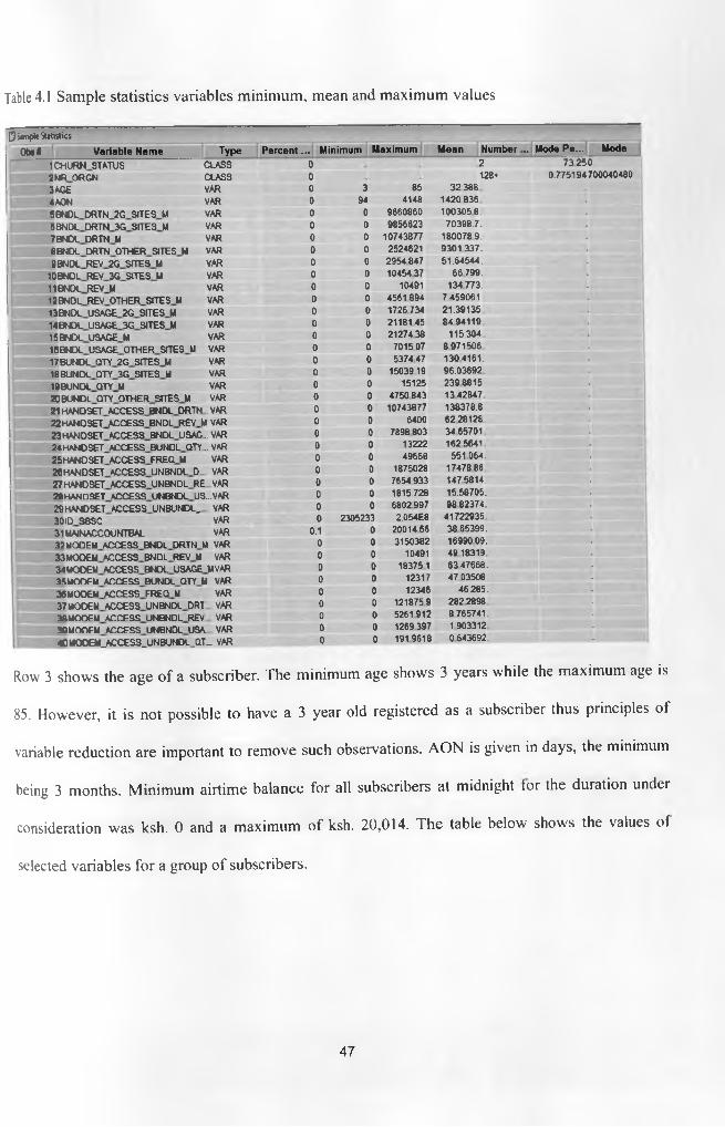
Table 4.1 Sample statistics variables minimum, mean and maximum values

0 Simple Statistics

0te« V a r ia b le N a m e T y p e P e r c e n t ... M in im um M ax im um M e a n Num ber .. M ode P e ... M ode

1 CHURN STATUS CLASS 0 2 73 2502 MR ORGN CLASS 0 .128+ 0.7751947000404803 AGE VAR 0 3 85 32 3884 AON VAR 0 94 4148 1420 8365BN0L DRTN 2G SITES M VAR 0 0 9660860 100305 8.6BNDL DRTN 3G SITES M VAR 0 0 9856623 70398.7.7BNDL DRTN M VAR 0 0 10743877 180078 9.8BNDL DRTN OTHER SITES M VAR 0 0 2524621 9301 337.9BNDL REV 2G SITES M VAR 0 0 2954 847 51.64544.10BNDL REV 3G SITES M VAR 0 0 1045437 66 799.11BNDL REV M VAR 0 0 10491 134 773.12BNDL REV OTHER SITES M VAR 0 0 4561 894 7 459061.13BNDL USAGE 2G SITES M VAR 0 0 1726734 21.3913514BNDL USAGE 3G SITES M VAR 0 0 21181 45 84 9411915BNDL USAGE M VAR 0 0 2127438 115.30416BNDL USAGE OTHER SITES M VAR 0 0 701507 8 97150617BUNDL QTY 2G SITES M VAR 0 0 537447 1304161.18 BUNDL QTY 3G SITES M VAR 0 0 15039 19 96.0369219BUNDL QTY M VAR 0 0 15125 239 8815.20BUNDL QTY OTHER SITES M VAR 0 0 4750 643 134284721 HANDSET ACCESS BNDL DRTN..VAR 0 0 10743877 138378.8.22 HANDSET ACCESS BNDL REV M VAR 0 0 6400 62 2812823 HANDSET ACCESS BNDL USAG..VAR 0 0 7898 803 34 6570124HANDSET ACCESS BUNDL QTY..VAR 0 0 13222 162 564125 HANDSET ACCESS FREQ M VAR 0 0 49668 551 064.26 HANDSET ACCESS UNBNDL D VAR 0 0 1875028 17478 8627 HANDSET ACCESS UNBNDL RE VAR 0 0 7654 933 147 5814.28HANDSET ACCESS UNBNDL US...VAR 0 0 1815.728 15.58705.29HANDSET ACCESS UNBUNDL_ VAR 0 0 6802997 98 82374.30 ID SBSC VAR 0 2305233 2.054E8 4172293531MAINACCOUNTBAL VAR 0.1 0 20014 66 38 65399.32 MODEM ACCESS BNDL DRTN M VAR 0 0 3150382 16990 09.33 MODEM ACCESS BNDL REV M VAR 0 0 10491 491831934MODEM ACCESS BNDL USAGE MVAR 0 0 183751 6347668. •

35 MODEM ACCESS BUNDL QTY M VAR 0 0 12317 47 03508.36MODEM ACCESS FREQ M VAR 0 0 12346 46.285. *37MODEM ACCESS UNBNDL DR1 VAR 0 0 1218759 282289838MODEM ACCESS UNBNDL REV VAR 0 0 5261 912 8 765741.39 MODEM ACCESS UNBNDL USA VAR 0 0 1269397 1 90331240 MOOEM_ACC£SS_UNBUNDL_Q1r_ VAR 0 0 191 9618 0 643692.

Row 3 shows the age of a subscriber. The minimum age shows 3 years while the maximum age is

85. However, it is not possible to have a 3 year old registered as a subscriber thus principles of

variable reduction are important to remove such observations. AON is given in days, the minimum

being 3 months. Minimum airtime balance for all subscribers at midnight tor the duration under

consideration was ksh. 0 and a maximum of ksh. 20,014. The table below shows the values of

selected variables for a group of subscribers.

47

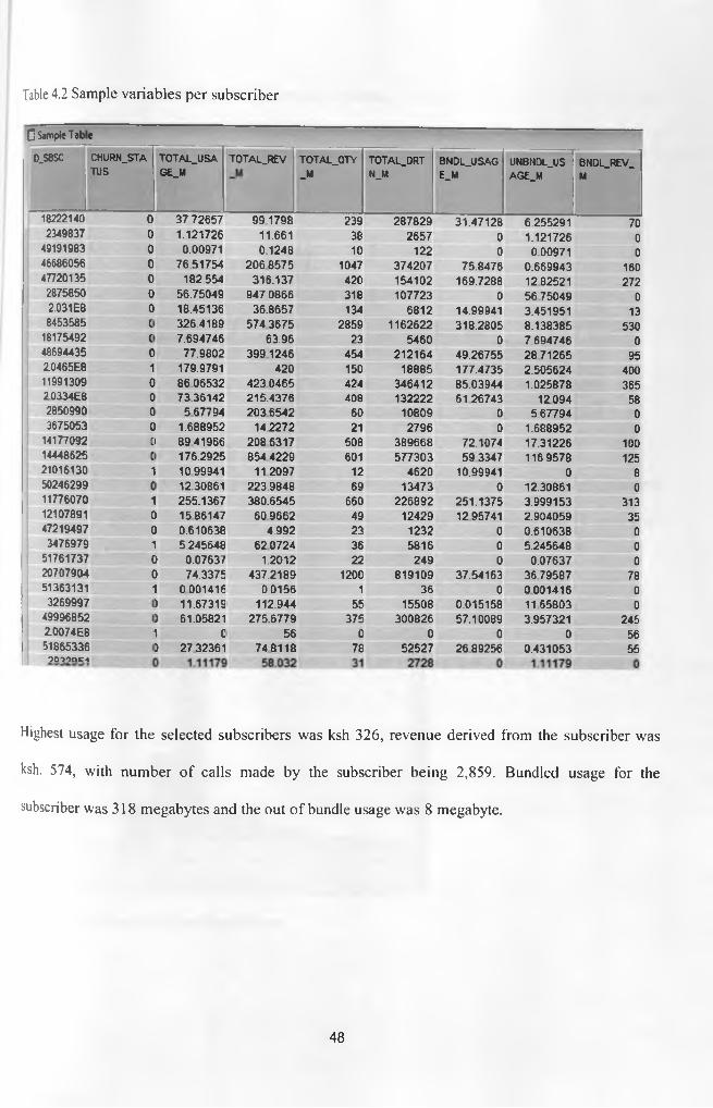
Table 4.2 Sample variables per subscriber

□ Sample TabeD.SBSC CHURN.STA

TUSTOTAL_USAGE_M

TOTAL.REV TOTAL.QTV_M

TOTAL_DRTN_M

BNDLJJSAGE_M

UNBNDLJJSAGE_M

BNDL_REV_M

18222140 0 37.72657 99 1798 239 287829 31.47128 6.255291 702349837 0 1.121726 11.661 38 2657 0 1.121726 049191983 0 0.00971 0.1248 10 122 0 0.00971 046686056 0 76.51754 206 8575 1047 374207 75.8476 0.669943 16047720135 0 182.554 316.137 420 154102 169.7288 1282521 2722875850 0 56.75049 947.0866 318 107723 0 5675049 02.031 E8 0 18.45136 36.8657 134 6812 14.99941 3.451951 138453585 c 326.4189 5743675 2859 1162622 318.2805 8.138385 53018175492 c 7.694746 63.96 23 5460 0 7.694746 048694435 0 77.9802 3991246 454 212164 49.26755 2871265 9520465E8 1 179.9791 420 150 18885 177.4735 2.505624 40011991309 0 8606532 4230465 424 346412 85.03944 1.025878 36520334E8 G 73.36142 215.4376 408 132222 61 26743 12094 582850990 G 5 67794 2036542 60 10809 0 5.67794 03675053 GI 1.688952 14.2272 21 2796 0 1.688952 0

14177092 CI 89 41966 2086317 508 389668 72.1074 17.31226 10014448625 c 176.2925 854 4229 601 577303 59 3347 116.9578 12521016130 1 1099941 11 2097 12 4620 10.99941 0 850246299 c 12.30861 223.9848 69 13473 0 12.30861 011776070 1I 255.1367 380.6545 660 226892 251.1375 3.999153 31312107891 0 1586147 609662 49 12429 1295741 2.904059 3547219497 0 0.610638 4.992 23 1232 0 0.610638 03476979 1 5.245648 620724 36 5816 0 5.245648 0

51761737 0 0.07637 1.2012 22 249 0 0.07637 020707904 0 74.3375 437.2189 1200 819109 37.54163 3679587 7851363131 1 0001416 0.0156 1 36 0 0001416 03269997 ) 11.67319 112.944 55 15508 0.015158 1165803 0

49996852 3 61.05821 275.6779 375 300826 57.10089 3.957321 2452.0074E8 1 G 56 0 0 0 0 5651865336ooioam 3 27 32361 74 8118 78 52527 2689256 0.431053 55

Highest usage for the selected subscribers was ksh 326, revenue derived from the subscriber was

ksh. 574, with number of calls made by the subscriber being 2,859. Bundled usage for the

subscriber was 318 megabytes and the out of bundle usage was 8 megabyte.

48

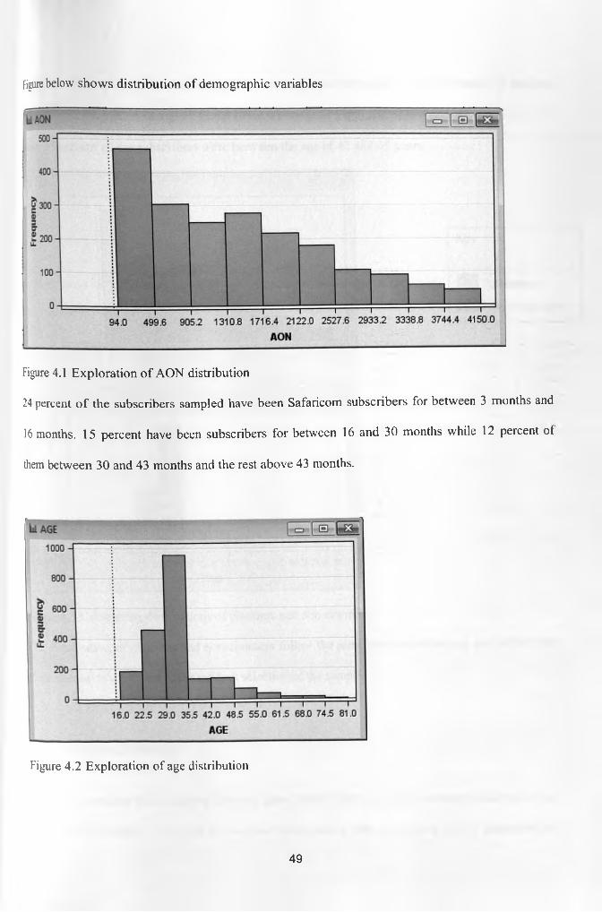
Figure below shows distribution of demographic variables

Figure 4.1 Exploration of AON distribution

24 percent o f the subscribers sampled have been Safaricom subscribers for between 3 months and

16 months. 15 percent have been subscribers for between 16 and 30 months while 12 percent ol

them between 30 and 43 months and the rest above 43 months.

Figure 4.2 Exploration of age distribution

49

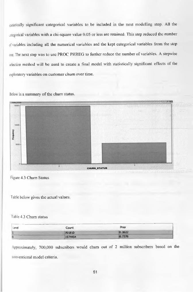
statistically significant categorical variables to be included in the next modelling step. All the

categorical variables with a chi-square value 0.05 or less are retained. This step reduced the number

of variables including all the numerical variables and the kept categorical variables from the step

one. The next step was to use PROC PH REG to further reduce the number of variables. A stepwise

selection method will be used to create a final model with statistically significant effects of the

exploratory variables on customer chum over time.

Below is a summary o f the chum status.

Figure 4.3 Chum Status

Table below gives the actual values.

Table 4.3 Chum status

level Count Prior701810 0.2622

• 1974454 0.7378

Approximately, 700,000 subscribers would chum out of 2 million subscribers based on the

conventional model criteria.

51

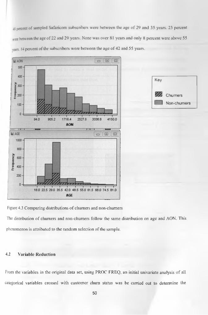
4$ percent of sampled Safaricom subscribers were between the age of 29 and 35 years. 23 percent

note between the age of 22 and 29 years. None was over 81 years and only 8 percent were above 55

.cars. 14 percent of the subscribers were between the age of 42 and 55 years.

Key

v? ,

i i

Chumers

Non-chumers

Figure 4.3 Comparing distributions o f chumers and non-chumers

The distribution of chumers and non-chumers follow the same distribution on age and AON. This

phenomenon is attributed to the random selection of the sample.

4.2 Variable Reduction

From the variables in the original data set, using PROC FREQ, an initial univariate analysis of all

categorical variables crossed with customer chum status was be carried out to determine the

50

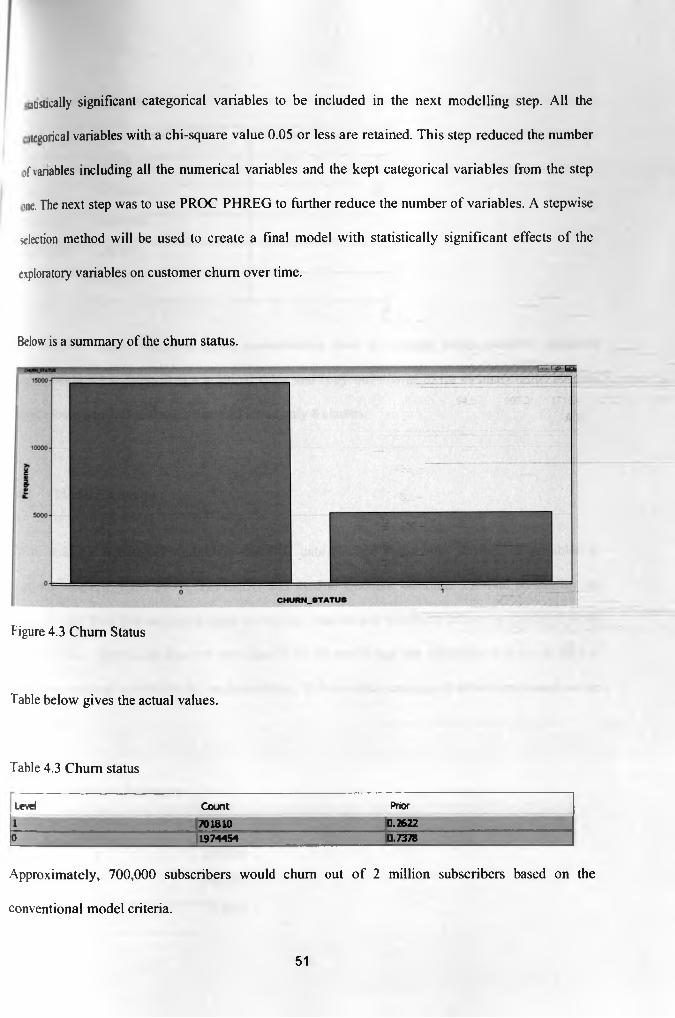
justically significant categorical variables to be included in the next modelling step. All the

:tecorical variables with a chi-square value 0.05 or less are retained. This step reduced the number

M'vanables including all the numerical variables and the kept categorical variables from the step

>ne. The next step was to use PROC PHREG to further reduce the number of variables. A stepwise

selection method will be used to create a final model with statistically significant effects of the

exploratory variables on customer chum over time.

Below is a summary of the chum status.

Figure 4.3 Chum Status

Table below gives the actual values.

Table 4.3 Chum status

Level Count Prior1 « ■ ■ ■ ■ ■ ■ ■ 701810 0.26220 1974454 0.7378

Approximately, 700,000 subscribers would chum out of 2 million subscribers based on the

conventional model criteria.

51

Table 4.4 Variables Summary

Role Measurement Level Frequency Count

ID INTERVAL 1

INPUT INTERVAL 79

REJECTED NOMINAL 1

REJECTED UNARY 1

TARGET BINARY 1

ID identified each subscriber under consideration. Due to missing value criterion described

subscriber age was rejected as a nominal value and copy quantity of Skiza as unary value because

most subscribers had missing value and it had only 8 classes.

4.3 Model Estimation

With reduced exploratory variables, the final data set had reasonable number of variables to

perform analysis. Here, PROC LIFEREG was used to calculate customer survival probability. In

this step, the final data set was divided to training data set and validation data set at a ratio of 60:40

respectively. The model data set was used to fit the model and the validation data set is used to

score the survival probability for each customer. Below is the summary of subscribers based on the

partitions.

Table 4.5 Partition Summary

Type Number of Observations

DATA 2676264

TRAIN 1605757

VALIDATE 1070507

52

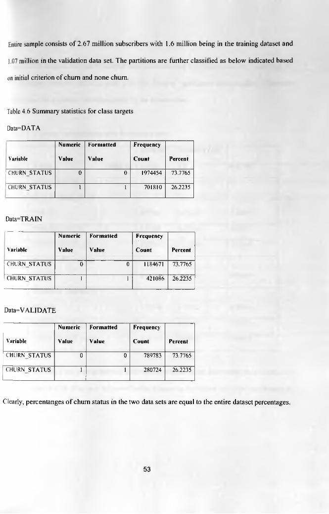
Entire sample consists of 2.67 million subscribers with 1.6 million being in the training dataset and

1.07 million in the validation data set. The partitions are further classified as below indicated based

on initial criterion of chum and none chum.

Table 4.6 Summary statistics for class targets

Data=DATA

Numeric Formatted Frequency

Variable Value Value Count Percent

CHURN STATUS 0 0 1974454 73.7765

CHURN STATUS 1 1 701810 26.2235

Data=TRAIN

Numeric Formatted Frequency

Variable Value Value Count Percent

CHURN STATUS 0 0 1184671 73.7765

CHURN STATUS 1 1 421086 26.2235

Data=VALIDATE

Numeric Formatted Frequency

Variable Value Value Count Percent

CHURN STATUS 0 0 789783 73.7765

CHURN STATUS 1 1 280724 26.2235

Clearly, percentanges of chum status in the two data sets are equal to the entire dataset percentages.

53

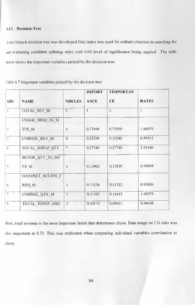
4.4.1 Decision Tree

A two branch decision tree was developed Gini index was used for ordinal criterion in searching for

and evaluating candidate splitting rules with 0.05 level of significance being applied. The table

below' shows the important variables picked by the decision tree.

Table 4.7 Important variables picked by the decision tree

OBS NAME NRULES

IMPORT

ANCE

VIMPORTAN

CE RATIO

1 TOTALREVM 2 1 1 1

2

USAGE_FREQ_2G_SI

TESM 5 0.73160 0.73510 1.00479

3 UNBNDLREVM 4 0.32398 0.32240 0.99513

4 TOTAL TOPUP QTY 7 0.27344 0.27740 1.01446

5

BUNDL_QTY_2G_SIT

ES_M 1 0.13962 0.13829 0.99049

6

HANDSETACCESSF

REQ M 1 0.13136 0.12322 0.93806

7 u n b n d l q t y m 1 0.11362 0.11415 1.00474

8 TOTAL TOPUP_AMT 3 0.10174 0.09831 0.96630

Here, total revenue is the most important factor that determines chum. Data usage on 2 G sites was

also important at 0.73. This was replicated when comparing individual variables contribution to

chum.

54

The other important variables include:

I. Revenue derived from out of bundle.

II. Top-up quantity.

III. Number of times 2G sites were used to browse internet.

IV. Use of handset to access internet.

V. Number of times of out of bundle usage.

VI. Top-up amount.

4.4.2 Cox proportional hazard model

Breslow method used to handle failure time’s ties. Below is the summary of events censored and

analysis of maximum likelihood estimates.

Table 4.8 Summary of Censored Events

Summary of the Number of Event and Censored

Values

Total Event Censored

Percent

Censored

1185984 658904 527080 44.44

44 percent of all the events were censored. This is according to time to chum based on the criteria

that chum occurs when one actually leaves the network.

55

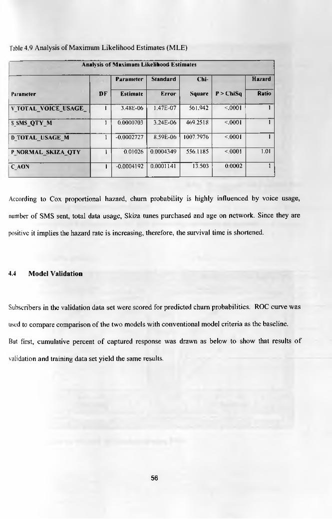
Table 4.9 Analysis of Maximum Likelihood Estimates (MLE)

Analysis of Maximum Likelihood Estimates

r—--------------------------------------------------------------------------------- Parameter Standard Chi- Hazard

Parameter D F Estimate Error Square P > ChiSq Ratio

\JOTAL_YOICE_USAGE_ 1 3.48E-06 1.47E-07 561.942 <.0001 1

S_SMS_QTY_M 1 0.0000703 3.24E-06 469.2518 <.0001 1

D_TOTALJJSAGE_M 1 -0.0002727 8.59E-06 1007.7976 <.0001 1

PNORMALSKIZAQTY ~ n 0.01026 0.0004349 556.1185 <.0001 1.01

C_AON i -0.0004192 0.0001141 13.503 0.0002 1

According to Cox proportional hazard, chum probability is highly influenced by voice usage,

number of SMS sent, total data usage, Skiza tunes purchased and age on network. Since they are

positive it implies the hazard rate is increasing, therefore, the survival time is shortened.

4.4 Model Validation

Subscribers in the validation data set were scored for predicted chum probabilities. ROC curve was

used to compare comparison of the two models with conventional model criteria as the baseline.

But first, cumulative percent of captured response was drawn as below to show that results of

validation and training data set yield the same results.

56

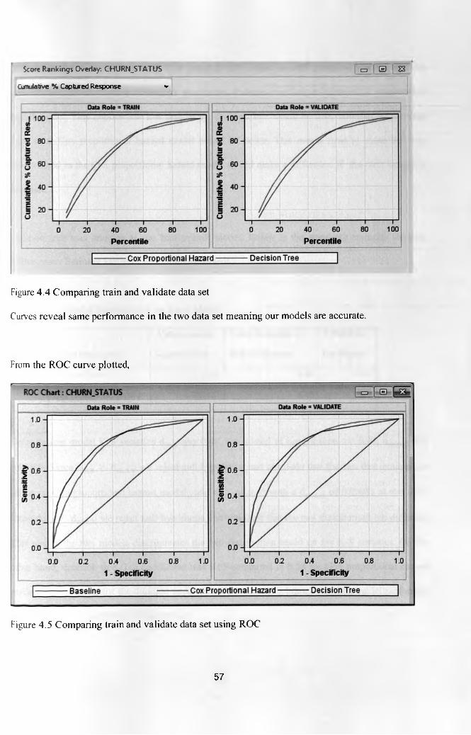
Score Rankings Overlay: CHURN.STATUS □ 0 [ S3

Cumulative % Captured Response ▼

Figure 4.4 Comparing train and validate data set

Curves reveal same performance in the two data set meaning our models are accurate.

From the ROC curve plotted,

Figure 4.5 Comparing train and validate data set using ROC

57

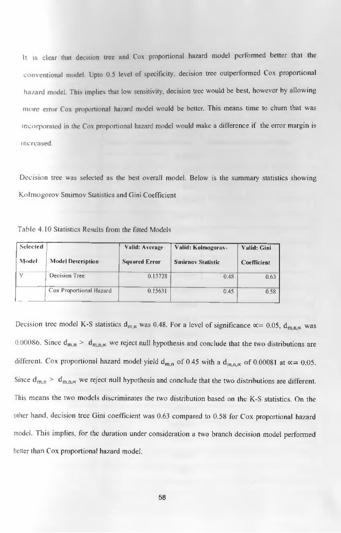
11 is clear that decision tree and Cox proportional hazard model performed better that the

conventional model. Upto 0.5 level of specificity, decision tree outperformed Cox proportional

hazard model. This implies that low sensitivity, decision tree would be best, however by allowing

more error Cox proportional hazard model would be better. This means time to chum that was

incorporated in the Cox proportional hazard model would make a difference if the error margin is

increased.

Decision tree was selected as the best overall model. Below is the summary statistics showing

Kolmogorov Smirnov Statistics and Gini Coefficient

Table 4.10 Statistics Results from the fitted Models

Selected Valid: Average Valid: Kolmogorov- Valid: Gini

Model Model Description Squared Error Smirnov Statistic Coefficient

Y Decision Tree 0.13728 0.48 0.63

Cox Proportional Hazard 0.15631 0.45 0.58

Decision tree model K-S statistics dm#n was 0.48. For a level of significance oc= 0.05, dm n oc was

0.00086. Since dm n > dm „ « we reject null hypothesis and conclude that the two distributions are

different. Cox proportional hazard model yield dm n of 0.45 with a dm n oc of 0.00081 at oc= 0.05.

Since d m<n > dm n oc we reject null hypothesis and conclude that the two distributions are different.

This means the two models discriminates the two distribution based on the K-S statistics. On the

other hand, decision tree Gini coefficient was 0.63 compared to 0.58 for Cox proportional hazard

model. This implies, for the duration under consideration a two branch decision model performed

better than Cox proportional hazard model.

58

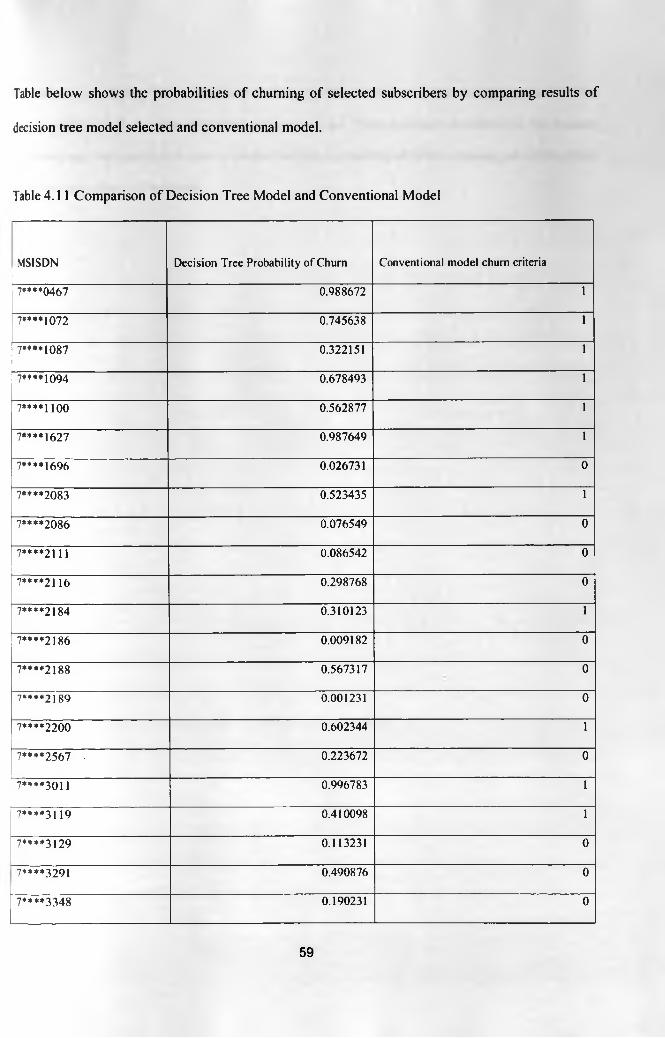
Table below shows the probabilities of churning of selected subscribers by comparing results of

decision tree model selected and conventional model.

Table 4.11 Comparison of Decision Tree Model and Conventional Model

MSISDN Decision Tree Probability of Churn Conventional model churn criteria

7****0467 0.988672 1

7**** 1072 0.745638 1

7****1087 0.322151 1

7**** 1094 0.678493 1

7****1100 0.562877 1

7****1627 0.987649 1

7****1696 0.026731 0

7****2083 0.523435 1

7****2086 0.076549 0

7****2111 0.086542 0

7****2116 0.298768 0

7****2184 0.310123 1

7****2186 0.009182 0

7****2188 0.567317 0

7****2189 0.001231 0

7****2200 0.602344 1

7****2567 0.223672 0

7****3011 0.996783 1

7****3119 0.410098 1

7****3129 0.113231 0

7****3291 0.490876 0

1****3348 0.190231 0

59

Decision tree model gives the probability of churning for the subscribers which is an improvement to initial

criteria which only shows if the subscriber will chum or not. There are some inconsistencies that decision

tree model selected improved on such as a subscriber had a probability of 0.56 of churning yet initial criteria

stated that subscriber will not chum.

60

l>cciston tree model gives the probability of churning for the subscribers which is an improvement to initial

entena which only shows if the subscriber will chum or not. There are some inconsistencies that decision

tree model selected unproved on such as a subscriber had a probability o f 0.56 o f churning yet initial criteria

stated that subscriber will not chum.

60

CHAPTER 5: CONCLUSIONS AND RECOMMENDATIONS

5,1 Conclusions

Current chum prediction methods used by Safaricom Limited are improved significantly by using

Cox proportional hazard and decision tree since there was a lift from the initial criteria on the ROC

curve. However, for the duration under consideration decision tree performed better than Cox

proportional model.

Decision tree gave probability o f chum which is an improvement from conventional model that

only gives binary results of chum and not churn. Also, where the decision tree yields approximately

50 percent probability of chum conventional model gave varying chum status.

5.2 Recommendations

To fully utilize the models, one has to run the models monthly. This would assist in continuously

tracking the behaviours of the subscribers as the behaviour patterns are affected by many

occurrences that cannot be controlled.

With monthly evaluation of propensity to chum, the impact of:

I. Executive management decision for example change of calling rates can be evaluated on the

impact of chum.

II. Competitor activities on propensity to chum can also be evaluated by running the models

monthly as we will be able to track propensity to chum per subscriber incorporating

competitor activities as our explanatory variable.

61

Other related models such as neural networks can be applied and compared to the results ol the

decision tree to further improve chum prediction.

62

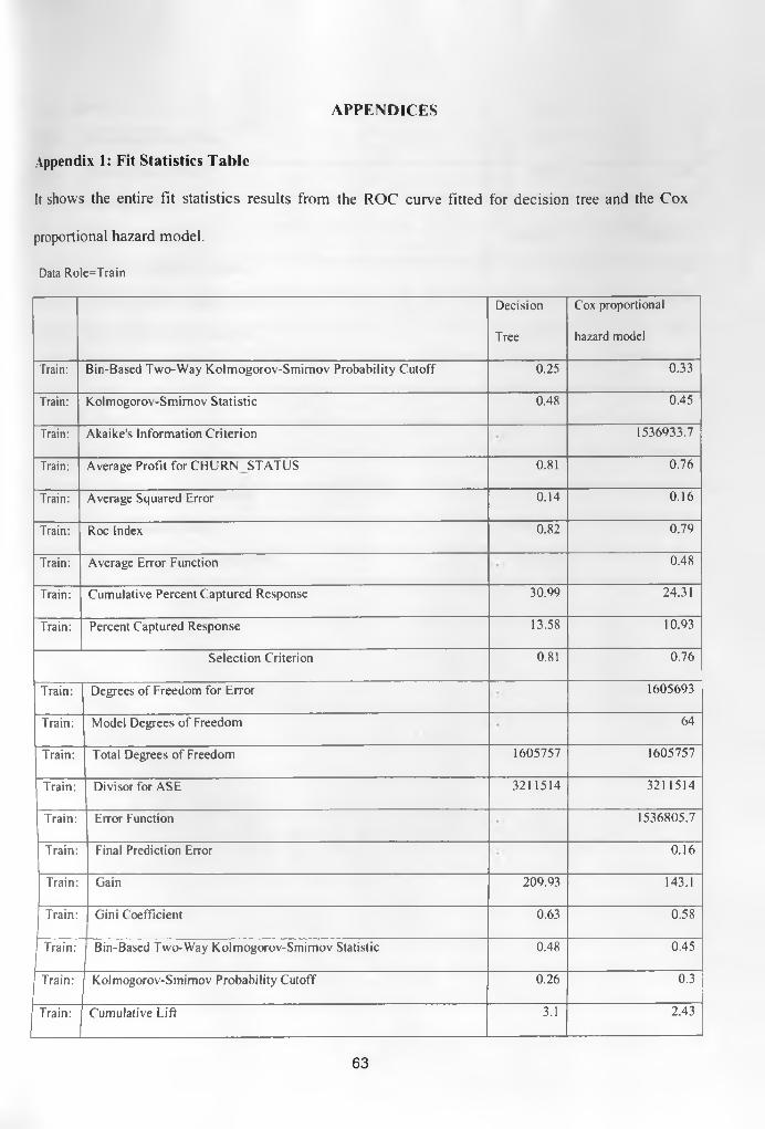
APPENDICES

Appendix 1: Fit Statistics Table

It shows the entire fit statistics results from the ROC curve fitted for decision tree and the Cox

proportional hazard model.

Data Role=Train

Decision

Tree

Cox proportional

hazard model

Train: Bin-Based Two-Way Kolmogorov-Smimov Probability Cutoff 0.25 0.33

Train: Kolmogorov-Smimov Statistic 0.48 0.45

Train: Akaike's Information Criterion 1536933.7

Train: Average Profit for CHURN STATUS 0.81 0.76

Train: Average Squared Error 0.14 0.16

Train: Roc Index 0.82 0.79

Train: Average Error Function 0.48

Train: Cumulative Percent Captured Response 30.99 24.31

Train: Percent Captured Response 13.58 10.93

Selection Criterion 0.81 0.76

Train: Degrees of Freedom for Error 1605693

Train: Model Degrees of Freedom 64

Train: Total Degrees of Freedom 1605757 1605757

Train: Divisor for ASE 3211514 3211514

Train: Error Function 1536805.7

Train: Final Prediction Error 0.16

Train: Gain 209.93 143.1

Train: Gini Coefficient 0.63 0.58

Train: Bin-Based Two-Way Kolmogorov-Smimov Statistic 0.48 0.45

Train: Kolmogorov-Smimov Probability Cutoff 0.26 0.3

Train: Cumulative Lift 3.1 2.43

63

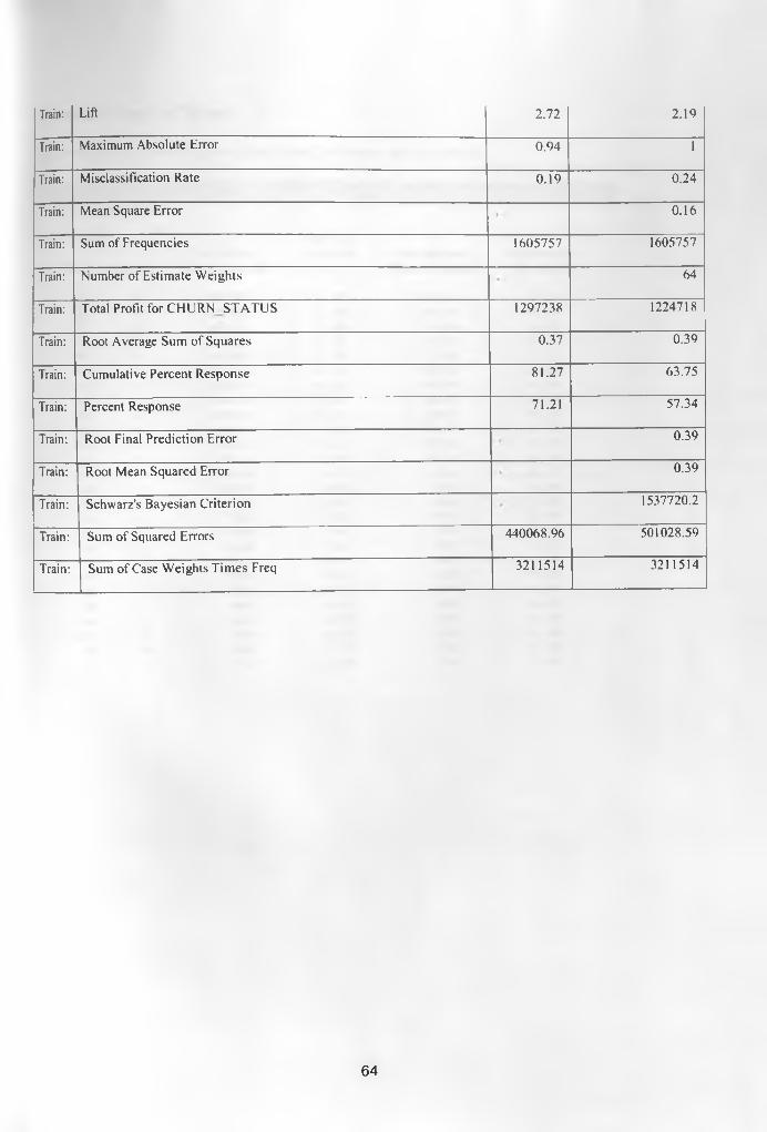
Train: Lift 2.72 2.19

Train: Maximum Absolute Error 0.94 1

Train: Misclassification Rate 0.19 0.24

Train: Mean Square Error 0.16

Train: Sum of Frequencies 1605757 1605757

Train: Number of Estimate Weights 64

Train: Total Profit for CHURN STATUS 1297238 1224718

Train: Root Average Sum of Squares 0.37 0.39

Train: Cumulative Percent Response 81.27 63.75

Train: Percent Response 71.21 57.34

Train: Root Final Prediction Error 0.39

Train: Root Mean Squared Error 0.39

Train: Schwarz's Bayesian Criterion 1537720.2

Train: Sum of Squared Errors 440068.96 501028.59

Train: Sum of Case Weights Times Freq 3211514 3211514

64

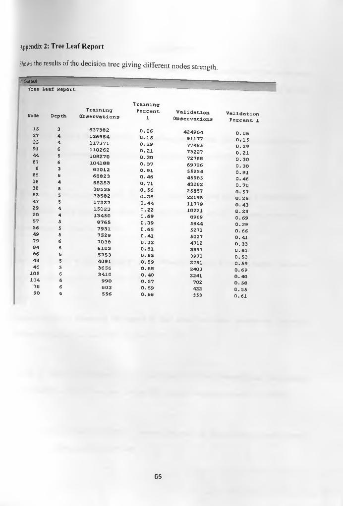
Appendix 2: Tree Leaf Report

Shows (he results of the decision tree giving different nodes strength.

Output

Tree Leaf Report

Rode DepthT ra in in g

Observations

T ra in in gPercent

1V a lid a t io n

ObservationsV alid at io n

Percent 1IS 3 637382 0.06 424964 0. 0627 4 136954 0.15 91177 0.1525 4 117371 0.29 77485 0.2991 6 110262 0.21 73227 0.2144 5 108270 0.30 72788 0.3087 6 104188 0.37 69726 0.388 3 83012 0.91 55254 0. 9185 6 68823 0.46 45985 0.4618 4 65253 0.71 43282 0.7038 5 38535 0.56 25857 0.5753 5 33582 0.26 22195 0.2547 5 17227 0 .44 11779 0.4329 4 15023 0.22 10221 0.2320 4 13450 0.69 8969 0. 6957 5 8765 0.39 5844 0.3956 5 7931 0.65 5271 0.6649 5 7529 0.41 5027 0.4179 6 7038 0.32 4712 0.3384 6 6103 0.61 3897 0.6186 6 5753 0.55 3978 0. 5348 5 4091 0.59 2751 0.5946 5 3656 0.68 2400 0.69105 6 3410 0.40 2241 0.40104 6 990 0.57 702 0. 5878 6 603 0.59 422 0.5590 6 556 0.66 353 0.61

65

Owczarczuk, M. (2009) Chum models for customers in the cellular telecommunication industry

using large data marts. Expert Systems w ith Applications, 37, 4710-4712

Seo, D., Ranganathan, C., and Badad, Y. (2008). Two-Level model of customer retention in US

mobile Telecommunication Service Market. Telecommunications Policy, 32, 182-196

Wei, C., and Chiu, I. (2002). Turning Telecommunications call details to chum prediction. Expert

Systems with Applications, 23, 103-112

Yan, L., Fassiono, M., and Baldasare, P. (2005). Predicting Customer Behaviour via calling links.

Proceeding o f International Joint Conference on Neural Networks, 4, 2555 - 2560

Yankee, G. (2001). Chum management in the mobile market. A Brazilian case study, 3, 202-16

67