CHPT03

Seediscussions,stats,andauthorprofilesforthispublicationat:http://www.researchgate.net/publication/252687357

Porepressureestimationinreservoirrocksfromseismicreflectiondata

ARTICLEinGEOPHYSICS·SEPTEMBER2003

ImpactFactor:1.61·DOI:10.1190/1.1620631

CITATIONS

12

READS

188

4AUTHORS,INCLUDING:

JoséMCarcione

OGSIstitutoNazionalediOceanografiaediGeofis…

335PUBLICATIONS3,493CITATIONS

SEEPROFILE

HansB.Helle

NationalLaboratoryforCivilEngineering

33PUBLICATIONS455CITATIONS

SEEPROFILE

TommyToverud

NorwegianUniversityofScienceandTechnology

9PUBLICATIONS72CITATIONS

SEEPROFILE

Availablefrom:JoséMCarcione

Retrievedon:28September2015

GEOPHYSICS, VOL. 68, NO. 5 (SEPTEMBER-OCTOBER 2003); P. 1569–1579, 12 FIGS., 2 TABLES.10.1190/1.1620631

Pore pressure estimation in reservoir rocks from seismic reflection data

Jose M. Carcione∗, Hans B. Helle‡, Nam H. Pham∗∗, and Tommy Toverud§

ABSTRACT

A method is used to obtain pore pressure in shaly sand-stones based upon an acoustic model for seismic velocityversus clay content and effective pressure. Calibrationof the model requires log data—porosity, clay content,and sonic velocities—to obtain the dry-rock moduli andthe effective stress coefficients as a function of depthand pore pressure. The seismic P-wave velocity, derivedfrom reflection tomography, is fitted to the theoreticalvelocity by using pore pressure as the fitting parame-ter. This approach, based on a rock-physics model, isan improvement over existing pore-pressure predictionmethods, which mainly rely on empirical relations be-tween velocity and pressure. The method is applied to theTune field in the Viking Graben sedimentary basin of theNorth Sea. We have obtained a high-resolution velocitymap that reveals the sensitivity to pore pressure and fluidsaturation in the Tarbert reservoir. The velocity map ofthe Tarbert reservoir and the inverted pressure distri-bution agree with the structural features of the TarbertFormation and its known pressure compartments.

INTRODUCTION

Knowledge of pore pressure using seismic data helps inplanning the drilling process—that is, casing and mud-weightdesign—to control potentially dangerous abnormal pressures.Proper pore-pressure prediction should involve the drilling en-gineer, the geologist, the geophysicist, and the petrophysicist,since the procedure requires mud-weight information, knowl-edge of the tectonic features of the area, use of seismic and welldata, and determination of petrophysical parameters relevantto the problem.

Let us introduce some useful definitions about the differentpressures considered in this work. Pore pressure, also known

Manuscript received by the Editor April 5, 2002; revised manuscript received January 27, 2003.∗Istituto Nazionale di Oceanografia e di Geofisica Sperimentale (OGS), Borgo Grotta Gigante 42c, 34010 Sgonico, Trieste, Italy. E-mail:[email protected].‡Norsk Hydro ASA, E&P Research Centre, Sandsliveien 90, N-5020 Bergen, Norway. E-mail: [email protected].∗∗Formerly Norwegian University of Science and Technology, Department of Petroleum Engineering and Applied Geophysics, N-7491 Trondheim,Norway; presently Statoil ASA, N-7501 Stjørdal, Norway. E-mail: [email protected].§Formerly Altinex ASA, N-5061 Kokstad, Norway; presently Norwegian University of Science and Technology, Department of PetroleumEngineering and Applied Geophysics, N-7491 Trondheim, Norway. E-mail: [email protected]© 2003 Society of Exploration Geophysicists. All rights reserved.

as formation pressure, is the in-situ pressure of the fluids in thepores. The pore pressure is equal to the hydrostatic pressurewhen the pore fluids support the weight of only the overlyingpore fluids (mainly water). The lithostatic or confining pres-sure results from the weight of overlying sediments, includingthe pore fluids. When the pore pressure attains the lithostaticpressure, the fluids support all of the weight. However, frac-tures perpendicular to the minimum compressive stress direc-tion appear for a given pore pressure, typically 70–90% of theconfining pressure. When fracturing occurs, the fluid escapesfrom the pores and pore pressure decreases. In addition, porepressure can decrease as a result of the presence of horizontalpermeability, which may prevent the development of overpres-sures. In normally pressured sedimentary basins, the effect ofa high sedimentation rate can be counteracted by horizontalpermeability effects and prevent compaction disequilibrium.

A rock is said to be overpressured when its pore pressureis significantly greater than hydrostatic pressure. The differ-ence between confining and pore pressures is called differentialpressure. Acoustic and transport properties of rocks generallydepend on effective pressure, a combination of pore and con-fining pressures [see equation (3)]. Various physical processescause anomalous pressures on an underground fluid. The mostcommon causes of overpressure are compaction disequilibriumand cracking, i.e., oil-to-gas conversion (Mann and Mackenzie,1990; Luo and Vasseur, 1996).

In general, nonseismic methods to predict pore pressureare based on a relation between porosity or void ratio andeffective stress (Bryant, 1989; Holbrook et al., 1995; Audet,1996; Traugott, 1997). Indirect use of velocity information in-volves estimating of the porosity profile by using sonic-log data(Hart et al., 1995; Harrold et al., 1999). A measurement whiledrilling (MWD) technique is proposed by Lesso and Burgess(1986), based on mechanical drilling data [rock strength com-puted from rate of penetration (ROP), weight on bit (WOB),and torque (TOR)] and gamma-ray logs. Seismic data canbe used to predict abnormal pore pressures in advance of

1569

1570 Carcione et al.

drilling. In general, this prediction has been based on empiricalmodels relating pore pressure to sonic and/or seismic veloc-ity (Pennebaker, 1968; Eaton, 1972; Belotti and Giacca, 1978;Bilgeri and Ademeno, 1982; Dutta and Levin, 1990; Kan andSicking, 1994; Bowers, 1995; Eaton and Eaton, 1997; Sayerset al., 2000).

Unlike previous theories, we use a Biot-type three-phasetheory that considers the existence of two solids (sandgrains and clay particles) and a fluid. The theory, developed byCarcione et al. (2000), is generalized here to include the effectsof pore and confining pressure to estimate pore pressure fromseismic velocities. At low frequencies, this theory is a general-ization of Gassmann’s equation for shaly sandstones, based onfirst physical principles. The theory was verified using real mea-surements of compressional and shear-wave velocities versusporosity and clay content. The model predicts additional slowwaves, but they are not used for pressure prediction. Attenua-tion from mode conversion and other mechanisms is neglected.The method requires high-resolution velocity information,preferably obtained from seismic inversion techniques. As iswell known, interval velocities obtained from conventionalseismic processing are not reliable enough for accurate pore-pressure prediction (Sayers et al., 2000; Carcione and Tinivella,2001). Calibration of the model requires well information,that is, porosity and shale volume estimation, direct mea-surements of pore pressure, and sonic-log data. Laboratorymeasurements of P- and S-wave velocities on core samplesmay further improve the calibration process (Carcione andGangi, 2000a,b).

PORE-PRESSURE PREDICTION METHOD

The sand–clay acoustic model for shaly sandstones devel-oped by Carcione et al. (2000) yields the seismic velocities as afunction of clay (shale) content, porosity, saturation, dry-rockmoduli, and fluid and solid-grain properties. As stated in previ-ous works (Carcione and Gangi, 2000a,b), variations in seismicvelocity are mainly because the dry-rock moduli are sensitivefunctions of the effective pressure, with the largest changes oc-curring at low differential pressures. Explicit changes in poros-ity and saturation are important but have a lesser influence onwave velocities than changes in the moduli. This is because themoduli are highly affected by the contact stiffnesses betweengrains. In this sense, porosity-based methods can be highly un-reliable. In fact, variations of porosity for Navajo Sandstone,Weber Sandstone, and Berea Sandstone are only 1.7%, 7%,and 4.5%, respectively, for changes of the confining pressurefrom 0 to 100 MPa (Berryman, 1992).

To use the present theory to predict pore pressure, we needto obtain the expression of the dry-rock moduli versus effectivepressure. The calibration process should be based on well, geo-logical, and laboratory data—mainly sonic and density data—and porosity and clay content inferred from logging profiles.

Let us assume a rock at depth z. The lithostatic or confiningpressure pc can be obtained by integrating the density log. Weknow that

pc = g∫ z

0ρ(z′)dz′, (1)

where ρ is the density and g is the acceleration of gravity. Fur-thermore, the hydrostatic pore pressure pH is approximately

given by

pH = ρwgz, (2)

where ρw is the density of water.As a good approximation (Prasad and Manghnani, 1997),

compressional- and shear-wave velocities and compression andshear moduli depend on effective pressure pe:

pe = pc − np, (3)

where p is pore pressure and n is the effective stress coefficient,which can be different for velocities and moduli (Christensenand Wang, 1985). Note that the effective pressure equals theconfining pressure at zero pore pressure. We find that n≈ 1for static measurements of the compressibilities (Zimmerman,1991), while n is approximately linearly dependent on the dif-ferential pressure pd = pc− p in dynamic experiments (Gangiand Carlson, 1996; Prasad and Manghnani, 1997). Therefore,we assume

n = n1 − n2 pd = n1 − n2(pc − p). (4)

This dependence of n versus differential pressure is in goodagreement with the experimental values corresponding to thecompressional velocity obtained by Christensen and Wang(1985) and Prasad and Manghnani (1997). Clearly to obtainn1 and n2 we need two evaluations of n at different pore pres-sures, preferably a normally pressured well and an overpres-sured well. Alternatively, n1 can be assumed equal to 1, andonly one evaluation is necessary in this case.

Calibration of the model

Ideally, a precise determination of n requires laboratory ex-periments on saturated samples for different confining andpore pressures. However, even this laboratory n does not re-flect the behavior of the rock at in-situ conditions for two mainreasons. First, laboratory measurements of wave velocity areperformed at ultrasonic frequencies Second, the in-situ stressdistribution is different from the stress applied in the experi-ments.

No laboratory experiments available.—In the absence of lab-oratory data, or for shales, we perform the following steps withthe data available from a calibration well.

First, we consider the model of Krief et al. (1990) to obtain anestimate of the dry-rock moduli Ksm, µsm (sand matrix), Kcm,and µcm (clay matrix) versus porosity and clay content. Theporosity dependence of the sand and clay matrices should beconsistent with the concept of critical porosity (Mavko et al.,1998, p. 244) since the moduli should vanish above a certainvalue of the porosity (usually from 0.4 to 0.5). This dependenceis determined by the empirical coefficient A [see equation (5)].This relation is suggested by Krief et al. (1990) and is appliedto sand–clay mixtures by Goldberg and Gurevich (1998). Thebulk and shear moduli of the sand and clay matrices are givenby, respectively,

Ksm(z) = Ks[1− C(z)][1− φ(z)]1+A/[1−φ(z)],

Kcm(z) = KcC(z)[1− φ(z)]1+A/[1−φ(z)],

Pore Pressure from Seismic Data 1571

µsm(z) = Ksm(z)µs

Ks,

µcm(z) = Kcm(z)µc

Kc, (5)

where Ks and µs are the bulk and shear moduli of the sandgrains and where Kc and µc those of the clay particles. Kriefet al. (1990) set the A parameter to three regardless of thelithology, and Goldberg and Gurevich (1998) obtain valuesbetween two and four, while Carcione et al. (2000) use two.Alternatively, the value of A can be estimated by using re-gional data from the study area. We use a general form of Gold-berg and Gurevich’s equation. Experimental data are fitted inCarcione et al. (2000), showing that the model has been testedsuccessfully. The model is not based on a dual porosity theory;rather, there is only one (connected) porosity. The clay mod-uli are taken from fit to experimental data in Goldberg andGurevich’s paper.

Second, we assume the following functional form for thedry-rock moduli as a function of effective pressure:

M(z) = α(z)[1− exp(−pe/p∗(z))], (6)

where α(z) and p∗(z) are parameters that should be obtained(for each moduli) by fitting Krief et al.’s expressions (5). Ini-tially, we assume that the effective pressure at depth z ispe= pc− p (Zimmerman, 1991, p. 43; Carcione, 2001, p. 233),where pc is given by equation (1) and p are taken from theformation pressure data in the calibration wells (see Figure 7).Since there are two unknown parameters (α and p∗) and onevalue of M for each depth, α(z) is assumed to be equal to theHashin-Shtrikman (HS) upper bounds (Hashin and Shtrikman,1963; Mavko et al., 1998, p. 106):

KHS(z) ={

Ks + φ(z)[

(1−φ(z))(

Ks + 43µs

)−1

− K−1s

]−1}(7)

and

µHS(z) = µs

{1+ 5φ(z)

[2(1− φ(z))(Ks + 2µs)

×(

Ks + 43µs

)−1

− 5]−1}

. (8)

Note that the HS lower bounds are zero and that the Voigtbounds are (1−φ)Ks and (1−φ)µs, respectively. For quartzgrains with clay, Ks= 39 GPa and µs= 33 GPa (Mavko et al.,1998, p. 307). If the limit porosity is 0.2, the HS upper boundsfor the bulk and shear moduli are 26 and 22 GPa, compared tothe Voigt upper bounds of 31 and 26 GPa, respectively. How-ever, the HS bounds are still too large to model the moduliof in-situ rocks. These contain clay and residual water satura-tion, inducing a chemical weakening of the contacts betweengrains (Knight and Dvorkin, 1992; Mavko et al., 1998, p. 203).Figure 1 shows the dry-rock bulk modulus of several reser-voir rocks for different confining pressures (Zimmerman, 1991,p. 29, Table 3.1), compared to the HS upper bounds. The solidline represents the analytical curve (9). On the basis of these

data points, we apply a constant weight factor β = 0.8 to theHS bounds, a result of the softening effects.

Third, we compute the exponential coefficients [see equa-tion (6)] using the values of the moduli obtained in step one,the confining and (measured) pore pressures, and the effectivestress coefficients equal to one. For instance, equation (6) forthe sand matrix can be written as

Ksm(z)=βKHS[1− exp

(−pe/

p∗K (z))]

(9)

and

µsm(z)=βµHS[1− exp

(−pe/p∗µ(z))]. (10)

Thus,

p∗K (z)=−pe(z){ln[1− Ksm(z)/(βKHS(z))]}−1 (11)

and

p∗µ(z) = −pe(z){ln[1− µsm(z)/(βµHS(z))]}−1, (12)

where we assume the effective pressure is equal to the differ-ential pressure.

Let us estimate the error in determining p∗K . Partial differen-tiation of p∗K with respect to Ksm and pe implies that the errorin the determination of p∗K is

1p∗K =p∗Kpe

(p∗K1Ksm

KHS − Ksm+1pe

), (13)

where 1Ksm and 1pe are the errors corresponding toKsm and pe, respectively. Consider the following exam-ple: KHS= 30 GPa, 1Ksm= 1 GPa, and 1pe= 1 MPa. Forp∗K = 15 MPa (soft rock), the error is 4.5 MPa at pe= 50 MPaand 20 MPa at pe= 5 MPa; while for p∗K = 40 MPa (stiff rock),the error is 4.5 MPa at pe= 50 MPa and 5.1 MPa at pe= 5 MPa.Therefore, the analysis indicates that a better estimation of p∗Kis achieved at high effective pressures and stiff rocks, that is,using data from normally pressured wells.

The last step of the calibration process is to consider equa-tion (3) and obtain the effective stress coefficients nK (z) andnµ(z) by fitting the theoretical velocities (Carcione et al., 2000)to the corresponding sonic-log P-wave and S-wave velocities by

FIG. 1. Dry-rock bulk modulus of several reservoir rocksfor different confining pressure, compared to the HS upperbounds. The solid line represents the analytical curve equa-tion (9). The data are taken from Zimmerman (1991, Table 3.1).

1572 Carcione et al.

using expressions (6). First, we obtain nµ by fitting the S-wavevelocity because this velocity only depends on µsm. Then weobtain nK by fitting the P-wave velocity. If shear-wave veloc-ity data are unavailable, we assume nµ= 1. From the valuesof n obtained at the two wells, we obtain the linear law (4)for the geological unit under investigation. The values of claycontent and porosity away from the wells are assumed to beequal to those of the nearest well. Interpretation is requiredto follow the geological units laterally, as a function of depth,so the n profiles can be properly extrapolated. In this study,the clay-matrix moduli Kcm and µcm are given by Krief et al.’sequations (5), with no explicit dependence on pressure.

Note that the HS bounds do not depend on the size and shapeof the grain and pores. In this sense, the model has a generalcharacter. The only conditions are linearity, isotropy, and thelow-frequency approximation.

More precisely, we use the following data of the study area tocalibrate the model and obtain the effective stress coefficientprofile for the formations under consideration:

1) an estimate of the porosity profile φ(z) to use in Kriefet al.’s model (see below) and in the sand–clay acoustic model(from a series of logs using artificial neural networks; Helleet al., 2001, and Helle and Bhatt, 2002,

2) an estimate of the clay-content profile C(z) to use in Kriefet al.’s model (see below) and in the sand–clay acoustic model(shale volumes obtained from SP logs or gamma-ray logs orusing neural networks; Helle et al., 2001, and Helle and Bhatt,2002,

3) direct measurements of pore pressure p(z) from repeatformation tests and/or mud weights provided by the mud-logging operator, and

4) sonic-log information, that is, the P- and S-wave veloc-ity profiles VP(z) and VS(z) used to obtain nK and nµ for thewhole range of effective pressures by fitting the theoreticalwave velocities to VP and VS, where nK and nµ are the effec-tive stress coefficients corresponding to the dry-rock bulk andshear moduli, respectively.

Laboratory experiments available.—The evaluation can beimproved if laboratory data of dry-rock P- and S-wave veloci-ties are available; this serves to constrain the values of α and p∗

in equation (6). These sparse calibration points are based onsandstone or shaly sandstone cores, since dry measurements inshals are practically impossible to perform. If sandstone coresare available, we proceed as follows.

The upper limits (infinite confining pressure) and exponen-tial coefficients of the moduli are obtained by fitting the dry-rock moduli, which are calculated from the dry-rock wave ve-locities, while n is obtained from experiments on saturated sam-ples for different confining and pore pressures (Carcione andGangi, 2000a,b).

The seismic bulk moduli Ksm and µsm versus confining pres-sure can be obtained from laboratory measurements in drysamples. If VP(dry) and VS(dry) are the experimental compres-sional and shear velocities, the moduli are given approximatelyby

Ksm= (1− φ)ρs

(VP(dry)2 − 4

3VS(dry)2

)and

µsm= (1− φ)ρsVS(dry)2, (14)

where ρs is the grain density. We recall that Ksm is the rockmodulus at constant pore pressure, i.e., the case when the bulkmodulus of the pore fluid is negligible compared with the dry-rock bulk modulus, as, for example, air at room conditions.Then, we perform experiments on saturated samples for differ-ent confining and pore pressures to obtain the effective stresscoefficient n. Because these experiments yield the P- and S-wave velocities and because the effective stress coefficients ofwave velocity and wave moduli may differ from each other, weobtain n for

K = ρ(

V2P −

43

V2S

)and µ = ρV2

S, (15)

where K and µ are the undrained moduli.We continue with the last step of the preceding list. This

step should improve the determination of n, estimated withlaboratory experiments in the first step.

Pore-pressure calculation

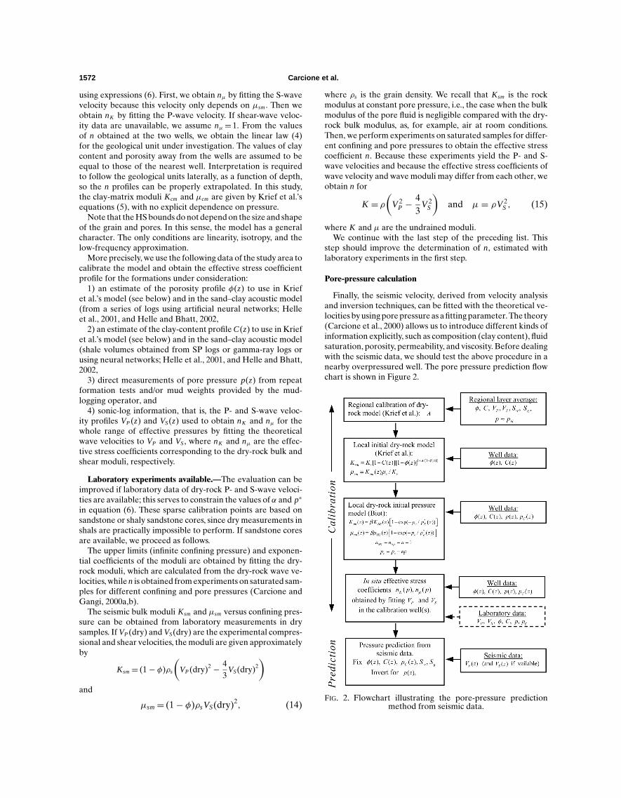
Finally, the seismic velocity, derived from velocity analysisand inversion techniques, can be fitted with the theoretical ve-locities by using pore pressure as a fitting parameter. The theory(Carcione et al., 2000) allows us to introduce different kinds ofinformation explicitly, such as composition (clay content), fluidsaturation, porosity, permeability, and viscosity. Before dealingwith the seismic data, we should test the above procedure in anearby overpressured well. The pore pressure prediction flowchart is shown in Figure 2.

FIG. 2. Flowchart illustrating the pore-pressure predictionmethod from seismic data.

Pore Pressure from Seismic Data 1573

AVO-based verification.—In some cases, velocity informa-tion alone is not enough to distinguish between a velocity inver-sion resulting from overpressure and a velocity inversion frompore fluid and lithology [e.g., base-of-salt reflections (Miley,1999; Miley and Kessinger, 1999)]. Occasionally, overpressur-ing is not associated with large velocity variations, as in smec-tite/illite transformations. Best et al. (1990) use AVO analy-sis to treat these cases. Modeling analysis of AVO signaturesof pressure transition zones is given in Miley (1999), Mileyand Kessinger (1999), and Carcione (2001). This type of anal-ysis should complement the present prediction method on thebasis of geological information of the study area.

EXAMPLE

We consider the Tune field area in the Viking Graben of theNorth Sea (Figure 3). This basin is 170–200 km wide and repre-sents a fault-bounded, north-trending zone of extended crust,flanked by the mainland of western Norway and the Shetlandplatform. The area is characterized by large normal faults withnorth, northeast, and northwest orientations that define tiltedblocks. Such blocks contain the sequences present within thewell used for this study. The main motivation for selecting thisarea is that highly overpressured compartments were identifiedby drilling and higher overpressure is expected in future wellsdown the flank side toward the west into the central VikingGraben. A general overview of the petroleum geology of theNorth Sea can be found in Glennie (1998), and a detailed anal-ysis of the fault sealing and pressure distribution in the Tunefield is given by Childs et al. (2002).

Figure 4 displays the simplified stratigraphic table, wherethe geological ages of the main stratigraphic boundaries areindicated. The Tune field is essentially a gas reservoir with athin layer of oil at its base. The reservoir is confined to theTarbert Formation, located in the upper section of the JurassicBrent Group, bounded by the shaly Heather Formation at thetop (seal) and by the Ness Formation below.

FIG. 3. Location of the Tune field in the Norwegian sector ofthe North Sea, offshore western Norway.

Figure 5 displays the time–structure map of the top Ness,showing faulting at a range of scales and orientations. On thewestern flank the reservoir terminates by a large fault planewhere the entire Brent is downfaulted by several hundred me-ters. Within the field a major southwest–northeast dip-slip faultdivides the Tarbert sand into two main compartments. Thisfault is expected to be crucial for sustaining the pressure dif-ferences in the field. Pressure data from wells on either side ofthe fault clearly indicate that the fault is a flow barrier, witha jump in pressure across the fault of 16 MPa. Wells 2 and 3in the downfaulted compartment (Figure 6) in the north areoverpressured (by about 15 MPa), and well 1 in the east com-partment has almost normal (hydrostatic) pore pressure. Thecalibration well (well 1) is an exploration well drilled to a depthof 3720 m (driller’s depth) to test the hydrocarbon potential ofthe Jurassic Brent Group. The well includes reservoir rocks ofthe Tarbert and Ness Formations, of which the Tarbert sandsare the target unit considered in the present study. A Kriefet al.’s parameter A= 3.15 is obtained by fitting sonic-log data.

FIG. 4. Stratigraphic table of the northern North Sea, show-ing the main stratigraphic boundaries. The target unit for thisstudy is the Tarbert Formation of the Jurassic Brent Group. Forgeological details see Glennie (1998).

1574 Carcione et al.

The 3D marine seismic data were acquired by using a sys-tem of six 3-km-long streamers with a group interval of 12.5 mand cross-line separation of 100 m. The shot spacing was 25 m,and the sampling rate 2 ms. The conventional stacked section isdisplayed in Figure 6, where the location of the wells is shown.Figure 7 shows pressure and formation data for the Tune wells.The shear-wave velocity in well 3 is obtained by using the em-pirical relation VS=−791.75+ 0.76535 VP (m/s), obtained byfitting data from nearby wells. Note that well 1 is water bearingwith almost normal pore pressures, while wells 2 and 3 are gasbearing and overpressured.

Velocity determination by tomography of depth-migratedgathers

Recent advances in depth migration have improved sub-surface model determination based on reflection seismology.

FIG. 5. Time–structure map of top Ness (base reservoir), show-ing the pressure compartments in the study area. Wells 2 and 3are overpressured (by about 15 MPa). In Well 1 there is almostnormal (hydrostatic) pore pressure. The blue line indicates thelocation of the seismic section shown in Figure 6. Notice thatwell 3 is highly deviated, as indicated by the well location atsurface (white star) and at total depth (white bullet).

FIG. 6. Seismic section through Tune wells (Figure 5), showingthe location of the top Tarbert–top Ness interval. The meanreservoir fluid pressures are indicated. The depths of interestare between top Tarbert (green) and top Ness (pink).

FIG. 7. Pressure and formation data: porosity φ, clay contentC, density ρ, water saturation Sw , and sonic-log velocities VPand VS for the Tune wells (see Figures 5 and 6 for location).

Pore Pressure from Seismic Data 1575

Subsurface imaging is linked to velocity, and an acceptable im-age can be obtained only with a highly accurate velocity field. Ithas been recognized that prestack migration is a powerful ve-locity analysis tool that yields better imaging results than post-stack migration in complicated structures. The basic assump-tion underlying the velocity determination methods based onprestack migration is that when the velocity is correct, all of themigrations with data in different domains (e.g., different off-set, different shots, different migration angles, etc.) must yielda consistent image.

To obtain the velocity field, we use the seismic inversion al-gorithm described by Koren et al. (1998). Figure 8 shows theflow chart of the velocity analysis procedure. We start with aninitial model based on the depth-converted time model, usinga layer velocity cube based on conventional stacking velocitiesand the interpreted time horizons from the Tune project. Lineby line, we perform the 3D prestack depth migration using theinitial velocity model and an appropriate aperture (3× 3 km at3 km depth) in the 3D cube covering an area of about 7× 20 km.Through several iteration loops the model is gradually refinedin velocity and hence depth. Each loop includes reinterpreta-tion of the horizons in the depth domain, residual moveoutanalysis, and residual moveout picks in the semblance volume.This is performed for each reflector of significance, starting atthe seabed and successively stripping the layers down to thetarget. The tomography considers (1) an initial velocity modeland (2) the errors as expressed by the depth gather residual

FIG. 8. Reflection tomography flowchart.

moveout and the associated 3D residual maps. From these twoinputs a new velocity model is derived where the layer depthsand layer velocities are updated iteratively to yield flat gathers.The refined model is derived using a tomographic algorithmthat establishes a link between perturbation in velocity andinterface location, and traveltime errors along the common re-flection point (CRP) rays traced across the model. CRP raysare ray pairs that obey Snell’s law and emanate from pointsalong the reflecting horizon, arriving at the surface with pre-defined offsets corresponding to the offset locations for themigrated gathers. Each pair establishes a relationship betweenthe CRP and the midpoint of the rays at the surface. Deptherrors, indicating the difference in depth of layer images andreference depth, are picked on the migrated gather along thehorizon and converted to time errors along the CRP rays.

In this study we use a layer-based tomography, where thesubsurface is described by a network of interlocking closedbodies best thought of as polygons rather than layers. Withineach polygon the velocity is represented by a laterally continu-ous function, while velocity changes discontinuously across thepolygon interface. Polygon velocities and thicknesses are up-dated in successive tomographic iterations. The objective is tofind both the interface locations and the lateral velocity func-tion within each polygon, which yields the flattest reflections inprestack migrated gathers (Kosloff et al., 1996). Layer-basedtomography makes use of the structural framework as a con-straint for interpolating velocity from one analysis point to theother. In the present situation, where velocities vary much lesswithin the layers than between them, this framework is an ef-fective constraint on interpolation. The equations relating thetime errors to changes in the model are solved by a weightedleast-squares technique.

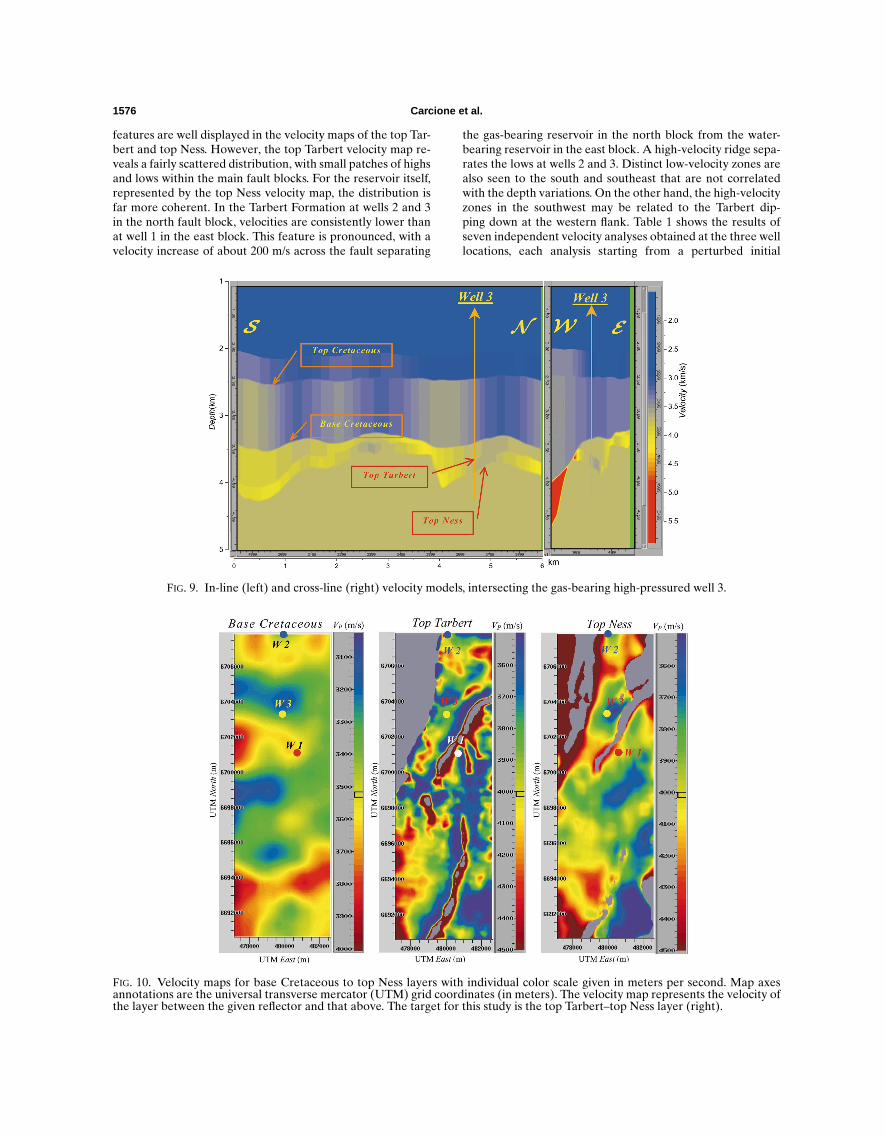
The final model consists of seven layers (see Figure 4), i.e., theseawater layer, seabed–top diapir (clay diapirism is a charac-teristic feature of Tertiary throughout the area), top diapir–topBalder, top Balder–top Cretaceous, top Cretaceous–base Cre-taceous, base Cretaceous–top Tarbert, and the target layer, topTarbert–top Ness. Figure 9 shows the in-line (left) and cross-line (right) velocity models, intersecting the gas-bearing high-pressure well 3.

The velocity maps for base Cretaceous (representing thevelocity of the layer between top Cretaceous and baseCretaceous), top Tarbert (representing the layer between baseCretaceous and top Tarbert), and top Ness (representing thelayer between top Tarbert and top Ness) are shown in Figure 10,where the well locations are indicated. This naming conventionhas been adopted because the seismic analysis focuses on CRPpoints at the base of the actual layer while the tomographicvelocities are those of the rocks between base and top.

The Cretaceous layer velocity and the depth to baseCretaceous (not shown) reveal a remarkable similarity, i.e.,where the Cretaceous is deep, the velocity is high; where theCretaceous is shallow, the velocity is low, indicating the velocityof Cretaceous is essentially governed by the overburden (e.g.,compaction). Whereas the structural features above the Creta-ceous are fairly smooth, the geometry at base Cretaceous andbelow is more dramatic, as is apparent from the seismic section(Figure 6). In the northwest flank the Tarbert and Ness Forma-tions terminate against the regional fault plane. Also, alongthe most significant local fault planes, the layers are undefined,and hence the discontinuity in the velocity maps. Structural

1576 Carcione et al.

features are well displayed in the velocity maps of the top Tar-bert and top Ness. However, the top Tarbert velocity map re-veals a fairly scattered distribution, with small patches of highsand lows within the main fault blocks. For the reservoir itself,represented by the top Ness velocity map, the distribution isfar more coherent. In the Tarbert Formation at wells 2 and 3in the north fault block, velocities are consistently lower thanat well 1 in the east block. This feature is pronounced, with avelocity increase of about 200 m/s across the fault separating

FIG. 9. In-line (left) and cross-line (right) velocity models, intersecting the gas-bearing high-pressured well 3.

FIG. 10. Velocity maps for base Cretaceous to top Ness layers with individual color scale given in meters per second. Map axesannotations are the universal transverse mercator (UTM) grid coordinates (in meters). The velocity map represents the velocity ofthe layer between the given reflector and that above. The target for this study is the top Tarbert–top Ness layer (right).

the gas-bearing reservoir in the north block from the water-bearing reservoir in the east block. A high-velocity ridge sepa-rates the lows at wells 2 and 3. Distinct low-velocity zones arealso seen to the south and southeast that are not correlatedwith the depth variations. On the other hand, the high-velocityzones in the southwest may be related to the Tarbert dip-ping down at the western flank. Table 1 shows the results ofseven independent velocity analyses obtained at the three welllocations, each analysis starting from a perturbed initial

Pore Pressure from Seismic Data 1577

velocity model. The standard deviation of 15 to 39 m/s indicatesthat errors in the tomographic velocity estimates are small com-pared with the lateral variation in the velocity field of about200 m/s and are in fair agreement with the P-wave velocitiesobtained by averaging the sonic logs over the reservoir section(Figure 6).

Application of the velocity model for pressure prediction

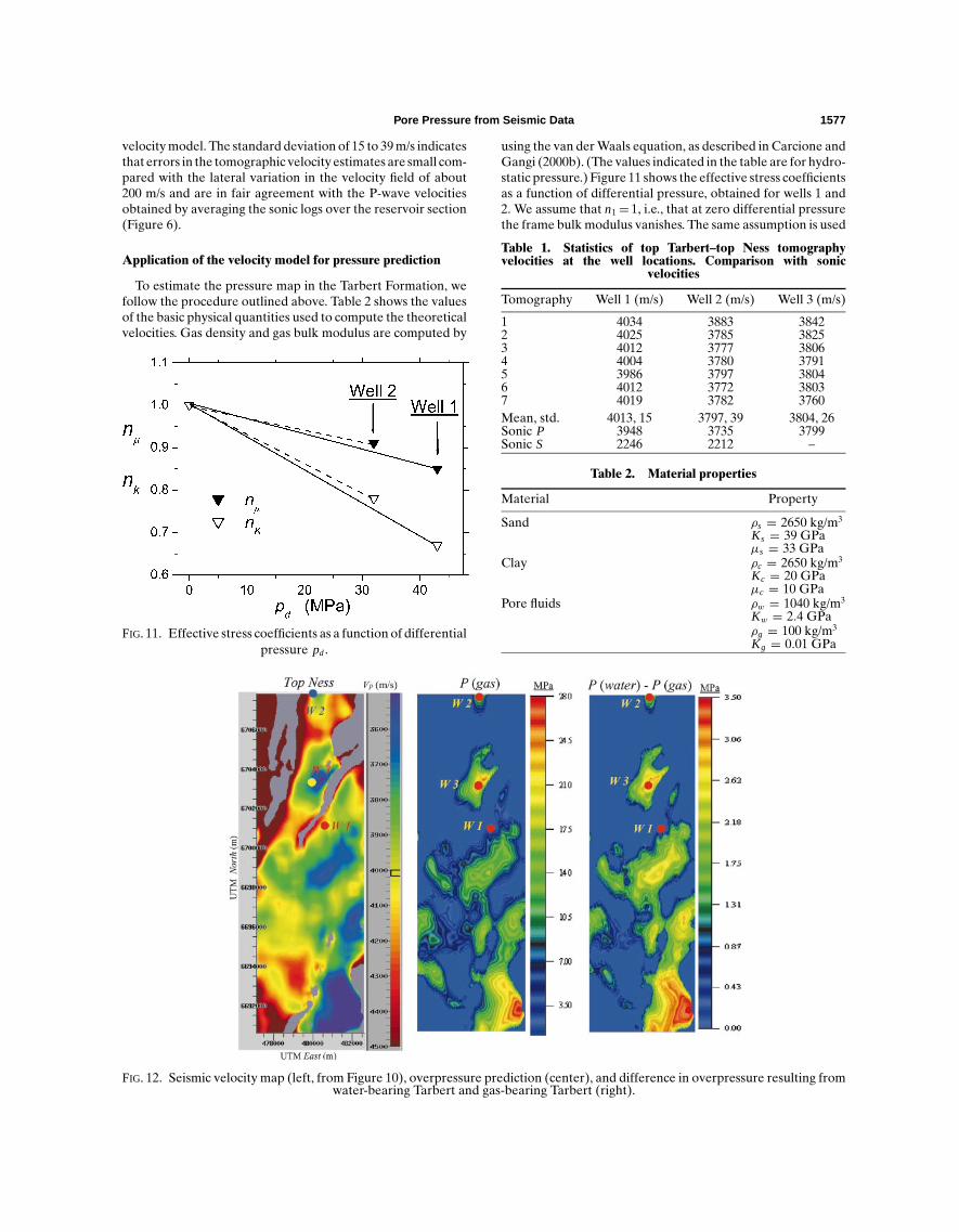
To estimate the pressure map in the Tarbert Formation, wefollow the procedure outlined above. Table 2 shows the valuesof the basic physical quantities used to compute the theoreticalvelocities. Gas density and gas bulk modulus are computed by

FIG. 11. Effective stress coefficients as a function of differentialpressure pd.

FIG. 12. Seismic velocity map (left, from Figure 10), overpressure prediction (center), and difference in overpressure resulting fromwater-bearing Tarbert and gas-bearing Tarbert (right).

using the van der Waals equation, as described in Carcione andGangi (2000b). (The values indicated in the table are for hydro-static pressure.) Figure 11 shows the effective stress coefficientsas a function of differential pressure, obtained for wells 1 and2. We assume that n1= 1, i.e., that at zero differential pressurethe frame bulk modulus vanishes. The same assumption is used

Table 1. Statistics of top Tarbert–top Ness tomographyvelocities at the well locations. Comparison with sonic

velocities

Tomography Well 1 (m/s) Well 2 (m/s) Well 3 (m/s)

1 4034 3883 38422 4025 3785 38253 4012 3777 38064 4004 3780 37915 3986 3797 38046 4012 3772 38037 4019 3782 3760Mean, std. 4013, 15 3797, 39 3804, 26Sonic P 3948 3735 3799Sonic S 2246 2212 –

Table 2. Material properties

Material Property

Sand ρs = 2650 kg/m3

Ks = 39 GPaµs = 33 GPa

Clay ρc = 2650 kg/m3

Kc = 20 GPaµc = 10 GPa

Pore fluids ρw = 1040 kg/m3

Kw = 2.4 GPaρg = 100 kg/m3

Kg = 0.01 GPa

1578 Carcione et al.

for the effective stress coefficient related to the frame rigiditymodulus.

Figure 12 shows the velocity map (left) and the overpressuremap, assuming Sw = 0.35 and a gas saturation Sg= 0.65 (cen-ter). The picture at the right represents the difference in porepressure by assuming gas-bearing Tarbert (center) and water-bearing Tarbert (Sw = 0.94 and Sg= 0.06). An overpressure ofabout 15 MPa is predicted for well 2, while slightly higher over-pressure (18 MPa) is predicted for well 1. The direct measure-ments indicate overpressures of about 15 MPa (see Figure 7).Figure 12 (right) shows that the sensitivity of the model tofluid saturation is about 2.5 MPa. The results in Figure 12 sup-port the hypothesis that the three wells are drilled in three iso-lated pressure compartments. Although the pressures in wells 2and 3 are similar, the apparent high-velocity zone betweenthose wells may indicate the existence of an isolated compart-ment with lower pressure. A closer inspection of the faults inFigures 5 and 6 may support this interpretation.

CONCLUSIONS

The velocity obtained by careful analysis of prestack 3D datafrom the deep and complex Tarbert reservoir in the Tune fieldis sufficiently sensitive to pressure and pore fluid to performa meaningful analysis. The velocity and pressure distributioncomplies well with the structural features of the target andthe general geological understanding of the pressure compart-ments in the Tune field. The partial saturation model used forpressure prediction can be calibrated conveniently against welldata, provided that a complete set of logging data are availablefor the zone of interest. The most important part of the predic-tion process is determining the effective stress coefficients anddry-rock moduli versus effective pressure, since these proper-ties characterize the acoustic behavior of the rock. The inver-sion method based on the shaly sandstone model must fix someparameters while inverting the others. For instance, assumingthe reservoir and fluid properties (mainly, the saturation val-ues), formation pressure can be inverted. Conversely, assumingthe pore pressure, the saturations can be obtained. The latterimplies that this method may be used in reservoir monitoringwhere the pressure distribution is known while saturation, i.e.,the remaining hydrocarbon reserves, is uncertain.

The prediction method accounts for most of the causes ofvelocity variation, i.e., saturation, fluid type, pressure, poros-ity, and lithology. Velocity differences by themselves do notnecessarily imply pressure differences. In the present example,we have applied the method to the same stratigraphic unit.Thus, variations associated with lithology can be neglected inprinciple. The method can be useful as an inversion (predic-tion) technique in these situations. When many unknowns arepresent (saturation, fluid type, lithology), the method can beused as a modeling technique.

We have neglected velocity dispersion, which is not easy totake into account, since Q-factor measurements are rare anddifficult to obtain with enough reliability. When using labora-tory data for the calibration, the effect of velocity dispersioncan be significant (Pham et al., 2002).

ACKNOWLEDGMENTS

This work was financed in part by the European Union aspart of the Detection of Overpressure Zones with Seismic and

Well Data project and by the Norwegian Research Councilunder the PetroForsk program (N.H.P.). We are grateful toAlpana Bhatt (Norwegian University of Science and Technol-ogy) for providing porosity, clay content, and saturation datafrom logs using her neural-network algorithms, to Stein-ErikKristensen (Norsk Hydro) for help in seismic interpretation,and to Bruce Hart for a detailed review and useful suggestions.

REFERENCES

Audet, D. M., 1996, Compaction and overpressuring in Pleistocenesediments on the Lousiana shelf, Gulf of Mexico: Marine Petr. Geol.,13, 467–474.

Belotti, P., and Giacca, D., 1978, Seismic data can detect overpressurein deep drilling: Oil & Gas J., August 21, 76–85.

Berryman, J. G., 1992, Effective stress for transport properties of in-homogeneous porous rock: J. Geophys. Res., 97, 17409–17424.

Best, M. E., Cant, D. J., Mudford, B. S., and Rees, J. L., 1990, Canvelocity inversion help map overpressure zones? Examples froman offshore margin: 60th Ann. Internat. Mtg., Soc. Expl. Geophys.,Expanded Abstracts, 763–765.

Bilgeri, D., and Ademeno, E. B., 1982, Predicting abnormally pressuredsedimentary rocks: Geophys. Prosp., 30, 608–621.

Bowers, G. L., 1995, Pore pressure estimation from velocity data—Accounting for overpressure mechanisms besides undercompaction:Internat. Assn. Drill. Cont./Soc. Petr. Eng. Drilling Conf., SPEpaper 27488.

Bryant, T. M., 1989, A dual pore pressure detection technique:Internat. Assn. Drill. Cont./Soc. Petr. Eng. Drilling Conf., SPEpaper 18714.

Carcione, J. M., 2001, Amplitude variations with offset of pressure-sealreflections: Geophysics, 66, 283–293.

Carcione, J. M., and Gangi, A., 2000a, Non-equilibrium compactionand abnormal pore-fluid pressures: Effects on seismic attributes:Geophys. Prosp., 48, 521–537.

———2000b, Gas generation and overpressure: Effects on seismicattributes: Geophysics, 65, 1769–1779.

Carcione, J. M., and Tinivella, U., 2001, The seismic response to over-pressure: A modeling methodology based on laboratory, well andseismic data: Geophys. Prosp., 49, 523–539.

Carcione, J. M., Gurevich, B., and Cavallini, F., 2000, A generalizedBiot-Gassmann model for the acoustic properties of shaley sand-stones: Geophys. Prosp., 48, 539–557.

Childs, C., Manzocchi, T., Nell, P. A. R., Walsh, J. J., Strand, J. A.,Heath, A. E., and Lygren, T. H., 2002, Geological implicationsof a large pressure difference across a small fault in the VikingGraben, in Koestler, A. G., and Hunsdale, R., Eds., Hydrocar-bon seal quantification: Norweg. Petr. Soc., Special Publ. 11,127–139.

Christensen, N. I., and Wang, H. F., 1985, The influence of pore pres-sure and confining pressure on dynamic elastic properties of BereaSandstone: Geophysics, 50, 207–213.

Dutta, N. C., and Levin, F. K., 1990, Geopressure: Soc. Expl. Geophys.Eaton, B. A., 1972, Graphical method predicts geopressure worldwide:

World Oil, 186, No. 6, 51–56.Eaton, B. A., and Eaton, T. L., 1997, Fracture gradient prediction for

the new generation: World Oil, October, 93–100.Gangi, A. F., and Carlson, R. L., 1996, An asperity-deformation model

for effective pressure: Tectonophysics, 256, 241–251.Glennie, K. W., Ed., 1998, Petroleum geology of the North Sea: Black-

well Scientific Publications, Inc.Goldberg, I., and Gurevich, B., 1998, A semi-empirical velocity-

porosity-clay model for petrophysical interpretation of P- andS-velocities: Geophys. Prosp., 46, 271–285.

Harrold, T. W. D., Swarbick, R. E., and Goulty, N. R., 1999, Pore pres-sure estimation from mudrock porosities in tertiary basins, SoutheastAsia: AAPG Bull., 83, 1057–1067.

Hart, B. S., Flemings, P. B., and Desphande, A., 1995, Porosity andpressure: Role of compaction disequilibrium in the developmentof geopressures in a Gulf Coast Pleistocene basin: Geology, 23,45–48.

Hashin, Z., and Shtrikman, S., 1963, A variational approach to theelastic behavior of multiphase materials: J. Mech. Phys. Solids, 11,127–140.

Helle, H. B., and Bhatt, A., 2002, Fluid saturation from well logs usingcommittee neural networks: Petr. Geosci., 8, 109–118.

Helle, H. B., Bhatt, A., and Ursin, B., 2001, Porosity and permeabilityprediction from wireline logs using artificial neural networks—ANorth Sea case study: Geophys. Prosp., 49, 431–444.

Holbrook, P., Maggiori, D. A., and Hensley, R., 1995, Real time pore

Pore Pressure from Seismic Data 1579

pressure and fracture pressure determination in all sedimentarylithologies: Form. Eval., December, 215–222.

Kan, T. K., and Sicking, C. J., 1994, Pre-drill geophysical methods forgeopressure detection and evaluation in abnormal formation pres-sures, in Fertl, W. H., Chapman, R. E., and Holz, R. F., Eds., Studiesin abnormal pressure: Elsevier, 155–186.

Knight, R., and Dvorkin, J., 1992, Seismic and electrical properties ofsandstones at low saturations: J. Geophys. Res., 97, 17425–17432.

Koren, Z., Kosloff, D., Zackhem, U., and Fagin, S., 1998, Velocity modeldetermination by tomography of depth migrated gathers, in Fagin, S.,Ed., Model-based depth imaging: Soc. Expl. Geophys., Course NoteSeries 10, 119–130.

Kosloff, D., Sherwood, J., Koren, Z., Machet, E., and Falkovitz, Y.,1996, Velocity and interface determination by tomography of depthmigrated gathers: Geophysics, 61, 1511–1523.

Krief, M., Garat, J., Stellingwerff, J., and Ventre, J., 1990, A petro-physical interpretation using the velocities of P and S waves (fullwaveform sonic): The Log Analyst, 31, 355–369.

Lesso, W. G., Jr., and Burgess, T. M., 1986, Pore pressure and porosityfrom MWD measurements: Internat. Assn. Drlg Cont./Soc. Petr.Eng. Drilling Conf., SPE paper 14801.

Luo, X., and Vasseur, G., 1996, Geopressuring mechanism of organicmatter cracking: Numerical modeling: AAPG Bull., 80, 856–874.

Mann, D. M., and Mackenzie, A. S., 1990, Prediction of pore fluid

pressures in sedimentary basins: Marine Petr. Geol., 7, 55–65.Mavko, G., Mukerji, T., and Dvorkin, J., 1998, The rock physics hand-

book: Tools for seismic analysis in porous media: Cambridge Univ.Press.

Miley, M. P., 1999, Converted modes in subsalt seismic exploration:MS. thesis, Rice Univ.

Miley, M. P., and Kessinger, W. P., 1999, Overpressure prediction usingconverted mode reflections from base of salt: 60th Ann. Internat.Mtg., Soc. Expl. Geophys., Expanded Abstracts, 880-883.

Pennebaker, E., 1968, Seismic data indicate depth and magnitude ofabnormal pressures: World Oil, 166, No. 7, 73–78.

Pham, N. H., Carcione, J. M., Helle, H. B., and Ursin, B., 2002, Wavevelocities and attenuation of shaley sandstone as a function of porepressure and partial saturation: Geophys. Prosp., 50, 615–627.

Prasad, M., and Manghnani, M. H., 1997, Effects of pore and differ-ential pressure on compressional wave velocity and quality factor inBerea and Michigan Sandstones: Geophysics, 62, 1163–1176.

Sayers, C. M., Johnson, G. M., and Denyer, G., 2000, Predrill pore pres-sure prediction using seismic data: Internat. Assn. Drill. Cont./Soc.Petr. Eng. Drilling Conf., SPE paper 59122.

Traugott, M., 1997, Pore/fracture pressure determinations in deep wa-ter: World Oil, August, Deepwater Technology Supplement, 68–70.

Zimmerman, R. W., 1991, Compressibility of sandstones: Elsevier,Science Publ. Co., Inc.