Chapter 3 Processor Management Operating Systems

Welcome message from author
This document is posted to help you gain knowledge. Please leave a comment to let me know what you think about it! Share it to your friends and learn new things together.
Transcript

Chapter 3
Processor Management
Operating Systems
How Does Processor Manager Allocate CPU(s) to Jobs?
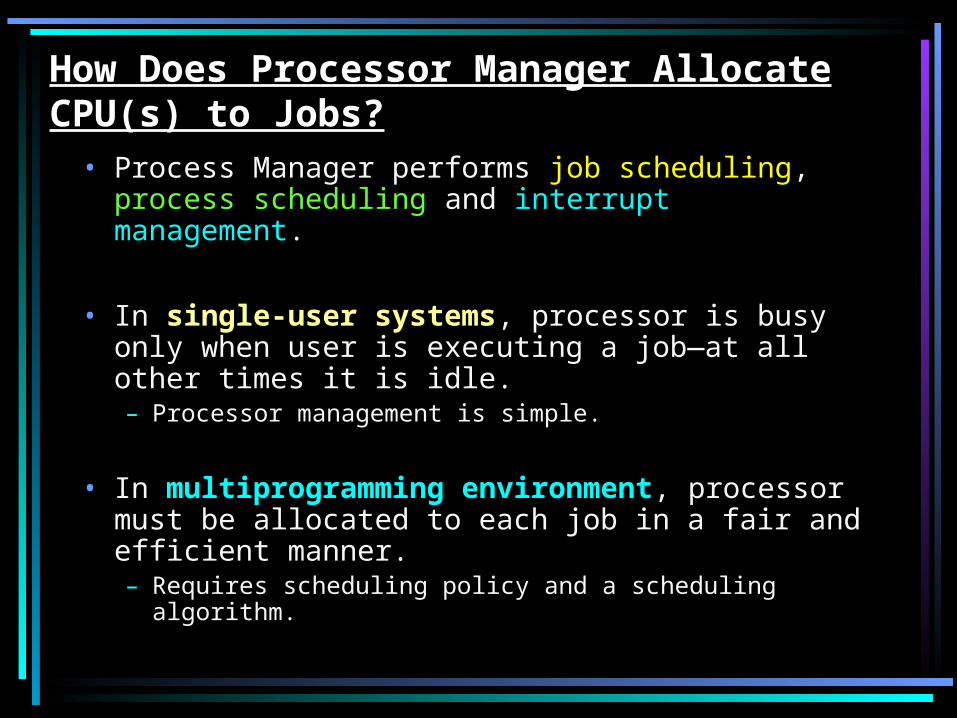
• Process Manager performs job scheduling, process scheduling and interrupt management.
• In single-user systems, processor is busy only when user is executing a job—at all other times it is idle. – Processor management is simple.
• In multiprogramming environment, processor must be allocated to each job in a fair and efficient manner.– Requires scheduling policy and a scheduling algorithm.

• Active multiprogramming is a time-sharing system which allows each program to use a preset slice of each CPU time. When the time expires, the job is interrupted and another job is allowed to begin.
• Passive multiprogramming allows each program to be serviced in turn, one after another by an interrupt. It ties up CPU time while all other jobs have to wait.

• Job Scheduling vs. Process Scheduling
• Processor Manager has 2 sub-managers:
• Job Scheduler– in charge of job scheduling.
• Process Scheduler– in charge of process scheduling.

Job Scheduler
•High-level scheduler.•Selects jobs from a queue of incoming jobs.•Places them in process queue (batch or interactive), based on each job’s characteristics.•Goal is to put jobs in a sequence that uses all system’s resources as fully as possible.•Strives for balanced mix of jobs with large I/O interaction and jobs with lots of computation. •Tries to keep most system components busy most of time.
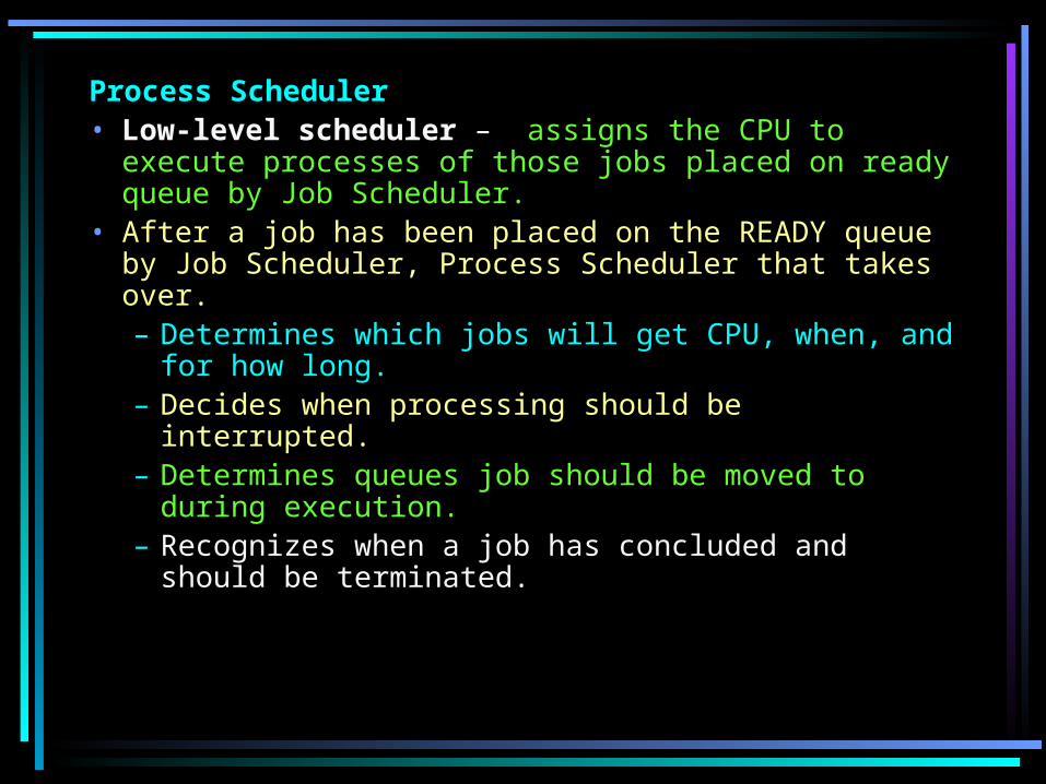
Process Scheduler• Low-level scheduler – assigns the CPU to
execute processes of those jobs placed on ready queue by Job Scheduler.
• After a job has been placed on the READY queue by Job Scheduler, Process Scheduler that takes over.– Determines which jobs will get CPU, when, and
for how long.– Decides when processing should be interrupted.– Determines queues job should be moved to
during execution.– Recognizes when a job has concluded and
should be terminated.

Schedulers
Disk Ready Queue CPU
I/OI/O waiting
Queue
End
Swap out
Swap outSw
ap in
Sw
ap in
Swapped out processes
Job Scheduler
Process Scheduler

CPU Cycles and I/O Cycles
• To schedule CPU, Process Scheduler uses common trait among most computer programs: they alternate between CPU cycles and I/O cycles.
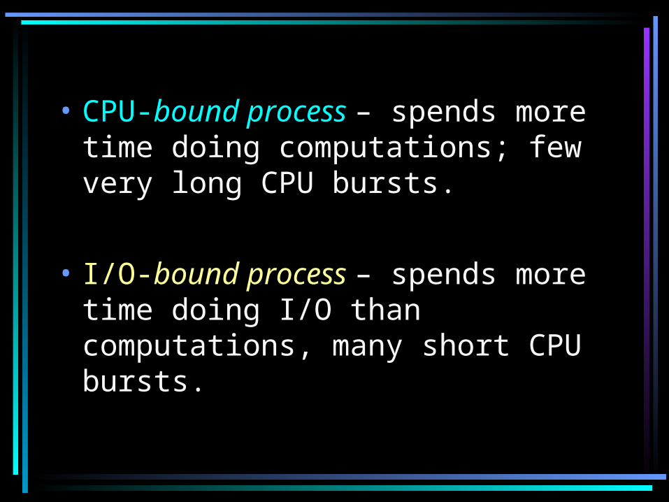
• CPU-bound process – spends more time doing computations; few very long CPU bursts.
• I/O-bound process – spends more time doing I/O than computations, many short CPU bursts.

I/O ModuleI/O ModuleI/O ModuleI/O ModuleI/O ModuleI/O Module
Computation
I/O ModuleI/O ModuleI/O ModuleI/O ModuleI/O Module
Computation
ComputationComputation
ComputationComputation
ComputationComputation
I/O Module
ComputationComputation
ComputationComputation
ComputationComputation
I/O Module
I/O-bound process CPU-bound process

READ A,B I/O cycle C = A+B D = (A*B)–C CPU cycle E = A–B F = D/E WRITE A,B,C,D,E,F I/O cycle STOP terminate execution END

• Middle-Level Scheduler
• In a highly interactive environment there’s a third layer– called middle-level scheduler.
• Removes active jobs from memory to reduce degree of multiprogramming and allows jobs to be completed faster

Middle-Level Scheduler
Disk Ready Queue CPU
I/OI/O waiting
Queue
End
Swap out
Swap outSw
ap in
Sw
ap in
Swapped out processes
Job Scheduler
Process Scheduler
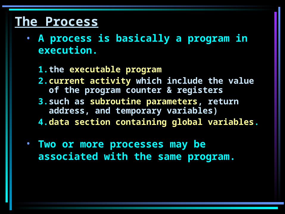
The Process• A process is basically a program in
execution.
1. the executable program2. current activity which include the value
of the program counter & registers3. such as subroutine parameters, return
address, and temporary variables)4. data section containing global variables.
• Two or more processes may be associated with the same program.

Process State
Hold/New
Ready Running
Waiting
Finish

Process State
• Hold/New: The process is being created.• Running: Instructions are being executed.• Waiting: The process is waiting for some
event to occur. (wait for I/O)• Ready: The process is waiting to be
assigned to a process. (waiting for CPU)
• Finish : The process has finished execution.
Process State
New/Hold
Ready Running
Waiting
Finish
Admitted
Interrupt
Schedulerdispatch
Exit
I/O or event wait
I/O Completion
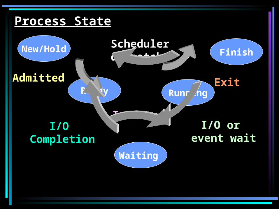
Transition among Process States
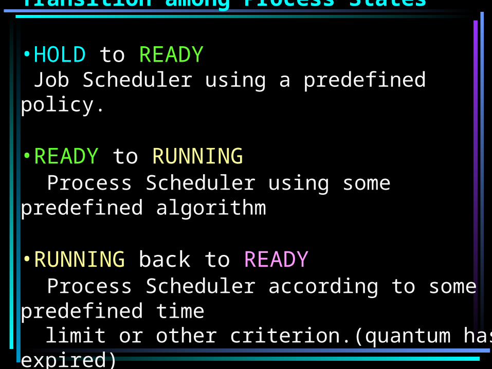
•HOLD to READY Job Scheduler using a predefined policy.
•READY to RUNNING Process Scheduler using some predefined algorithm
•RUNNING back to READY Process Scheduler according to some predefined time limit or other criterion.(quantum has expired)
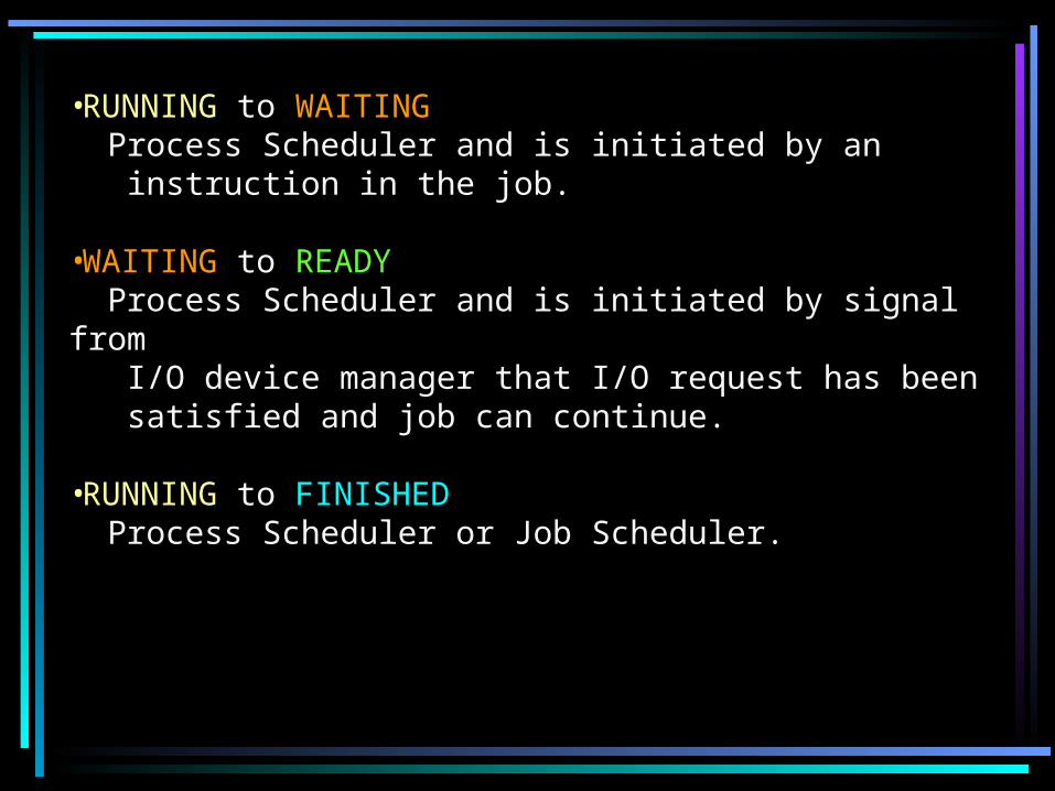
•RUNNING to WAITING Process Scheduler and is initiated by an instruction in the job.
•WAITING to READY Process Scheduler and is initiated by signal from I/O device manager that I/O request has been satisfied and job can continue.
•RUNNING to FINISHED Process Scheduler or Job Scheduler.

Process Control Block (PCB)
• Each process in the O/S is represented by a PCB repository for information that vary from process to other process

Process Control Block (PCB)
Process State
Program Counter
CPU Registers
CPU Scheduling Information
Memory Management Information
Accounting Information
I/O Status Information
New/Hold/Running/Wait/Ready/Finish
Address for next instruction
AC, IR and Stack pointer
Process Priority
Base and Limit Register
CPU Time Used
I/O devices allocated

Process Control Block (PCB)Process P0 Process P1
Save State into PCB0
Reload State from PCB1
Save State into PCB1
Reload State from PCB0
Interrupts or I/O executingidle
executingidle
idleexecuting

• PCBs and Queuing• PCB of job created when Job Scheduler accepts
it– Updated as job goes from beginning to
termination.• Queues use PCBs to track jobs.
– PCBs, not jobs, are linked to form queues.– E.g., PCBs for every ready job are linked on
READY queue; all PCBs for jobs just entering system are linked on HOLD queue.
– Queues must be managed by process scheduling policies and algorithms.
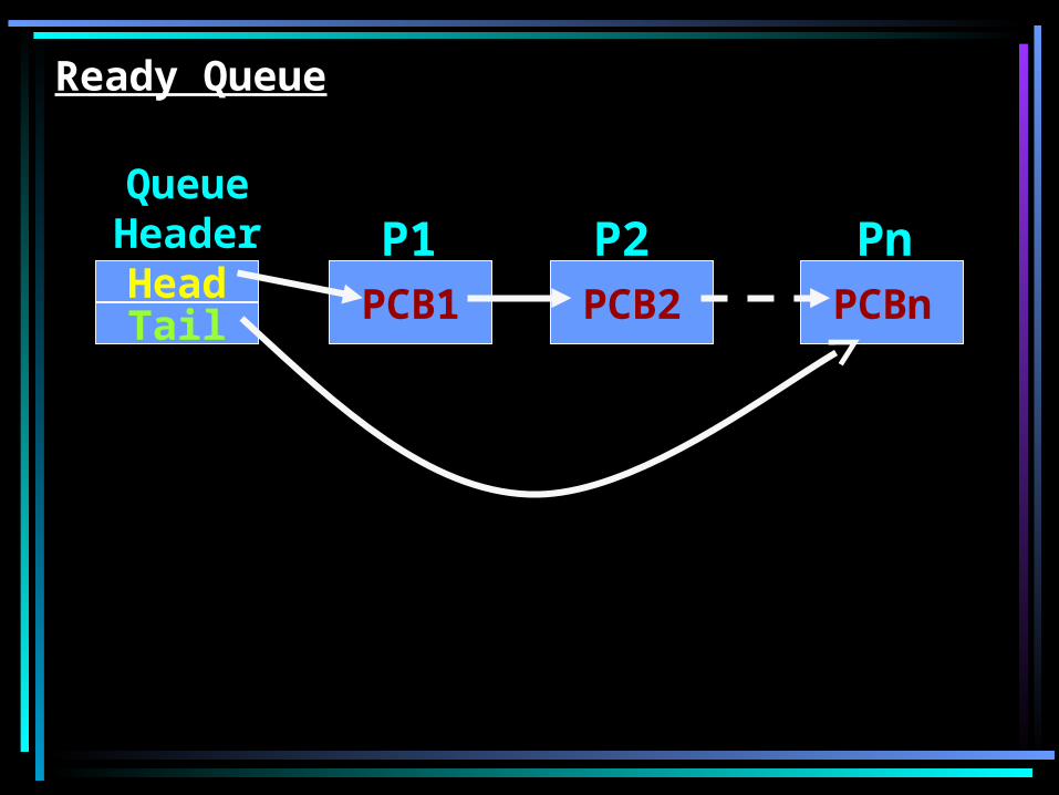
Ready Queue
PCB1 PCB2 PCBnHeadTail
Queue Header P1 P2 Pn

Process Scheduling Policies
• Before operating system can schedule all jobs in a multiprogramming environment, it must resolve three limitations of system: – finite number of resources (such as
disk drives, printers, and tape drives)– some resources can’t be shared once
they’re allocated (such as printers)– some resources require operator
intervention (such as tape drives).
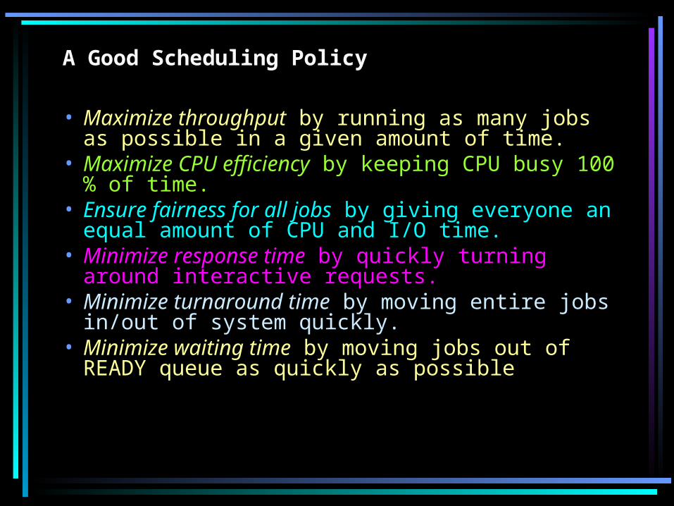
A Good Scheduling Policy
• Maximize throughput by running as many jobs as possible in a given amount of time.
• Maximize CPU efficiency by keeping CPU busy 100 % of time.
• Ensure fairness for all jobs by giving everyone an equal amount of CPU and I/O time.
• Minimize response time by quickly turning around interactive requests.
• Minimize turnaround time by moving entire jobs in/out of system quickly.
• Minimize waiting time by moving jobs out of READY queue as quickly as possible

Waiting Time (w) = Finish Time – Arrival Time – CPU Cycle
Turnaround Time (t) = Finish Time – Arrival Time

• Preemptive scheduling policy interrupts processing of a job and transfers the CPU to another job. (the Arrival process will interrupt the current process)
• Non-preemptive scheduling policy functions without external interrupts.– Once a job captures processor and begins
execution, it remains in RUNNING state uninterrupted until it issues an I/O request (natural wait) or until it is finished (exception for infinite loops).
– (current process cannot be preempted until completes its CPU cycle).
– (current process cannot be preempted until completes its CPU cycle).

Process Scheduling Algorithms • First Come First Served (FCFS) –non
preemptive
• Shortest Job Next (SJN)- non preemptive
• Shortest Remaining Time First (SRT) preemptive
• Round Robin- preemptive
• Priority Scheduling- preemptive• Priority Scheduling- non-preemptive
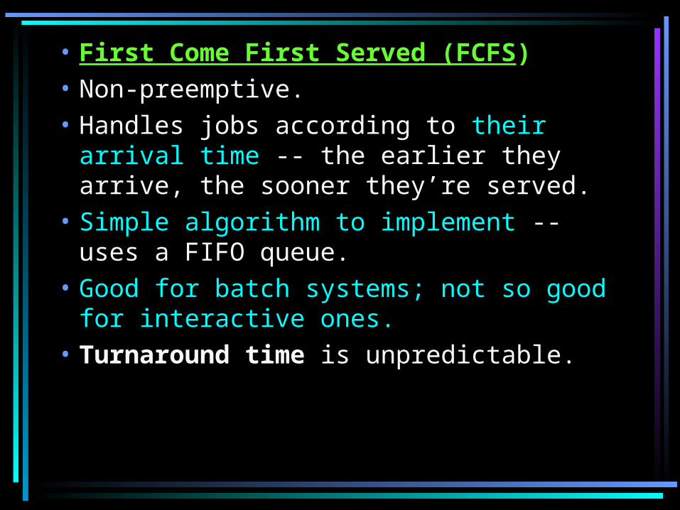
• First Come First Served (FCFS)• Non-preemptive.• Handles jobs according to their arrival
time -- the earlier they arrive, the sooner they’re served.
• Simple algorithm to implement -- uses a FIFO queue.
• Good for batch systems; not so good for interactive ones.
• Turnaround time is unpredictable.

To draw timeline and to do calculations for process scheduling algorithms
Job Arrival Time CPU Cycle
A 0 8
B 1 5
C 2 3
D 3 1
E 4 7
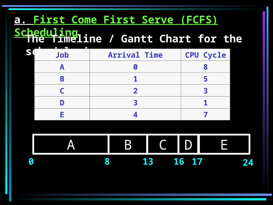
a. First Come First Serve (FCFS) Scheduling
The Timeline / Gantt Chart for the schedule is:
A B0 8 13 16
Job Arrival Time CPU Cycle
A 0 8
B 1 5
C 2 3
D 3 1
E 4 7
C D E17 24

a. First Come First Serve (FCFS) Scheduling
The Timeline / Gantt Chart for the schedule is:
A B0 8 13 16
C D E17 24
Waiting Time (w) = Finish Time – Arrival Time – CPU Cyclew(A) = 8 – 0 – 8 = 0
w(B) = 13 – 1 – 5 = 7w(C) = 16 – 2 – 3 = 11
w(D) = 17 – 3 – 1 = 13w(E) = 24 – 4 – 7 = 13
Average Waiting Time = Total Waiting Time / Total number of processes
Average Waiting Time = 44 / 5
Average Waiting Time = 8.8

a. First Come First Serve (FCFS) Scheduling
The Timeline / Gantt Chart for the schedule is:
A B0 8 13 16
C D E17 24
Turnaround Time (t) = Finish Time – Arrival Time
w(A) = 8 – 0 = 8
w(B) = 13 – 1 = 12w(C) = 16 – 2 = 14
w(D) = 17 – 3 = 14w(E) = 24 – 4 = 20
Average Turnaround Time = Total Turnaround Time / Total number of processes
Average Turnaround Time = 62 / 5Average Turnaround Time = 13.6
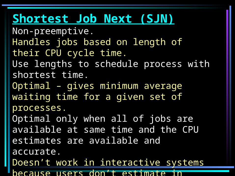
Shortest Job Next (SJN)Non-preemptive.Handles jobs based on length of their CPU cycle time. Use lengths to schedule process with shortest time.Optimal – gives minimum average waiting time for a given set of processes. Optimal only when all of jobs are available at same time and the CPU estimates are available and accurate.Doesn’t work in interactive systems because users don’t estimate in advance CPU time required to run their jobs.

b. Shortest Job Next (SJN) Scheduling (Non Preemption)
The Timeline / Gantt Chart for the schedule is:
A D0 8 9 12
Job Arrival Time CPU Cycle
A 0 8
B 1 5
C 2 3
D 3 1
E 4 7
C B E17 24

Waiting Time (w) = Finish Time – Arrival Time – CPU Cyclew(A) = 8 – 0 – 8 = 0
w(B) = 17 – 1 – 5 = 11w(C) = 12 – 2 – 3 = 7
w(D) = 9 – 3 – 1 = 5 w(E) = 24 – 4 – 7 = 13
Average Waiting Time = Total Waiting Time / Total number of processes
Average Waiting Time = 36 / 5
Average Waiting Time = 7.2
A D0 8 9 12
C B E17 24

Turnaround Time (t) = Finish Time – Arrival Time
w(A) = 8 – 0 = 8
w(B) = 17 – 1 = 16w(C) = 12 – 2 = 10
w(D) = 9 – 3 = 6w(E) = 24 – 4 = 20
Average Turnaround Time = Total Turnaround Time / Total number of processes
Average Turnaround Time = 60 / 5Average Turnaround Time = 12
A D0 8 9 12
C B E17 24
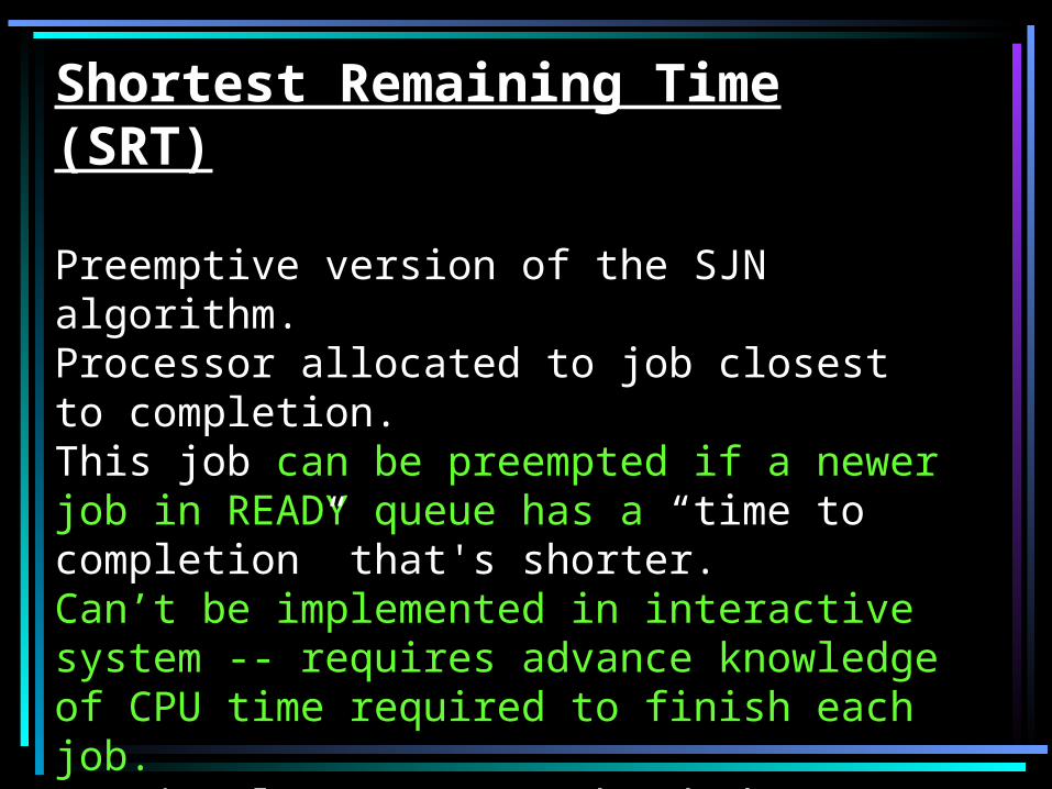
Shortest Remaining Time (SRT) Preemptive version of the SJN algorithm. Processor allocated to job closest to completion.This job can be preempted if a newer job in READY queue has a “time to completion” that's shorter.Can’t be implemented in interactive system -- requires advance knowledge of CPU time required to finish each job. SRT involves more overhead than SJN. OS monitors CPU time for all jobs in READY queue and performs “context switching”.
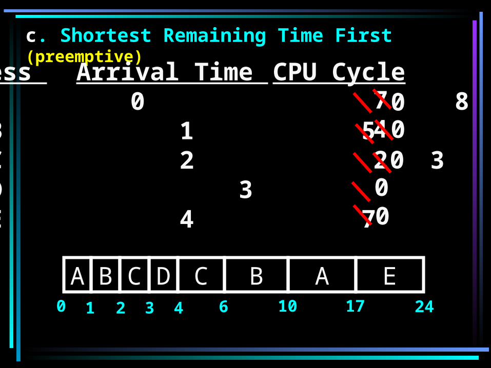
c. Shortest Remaining Time First (preemptive)
Process Arrival Time CPU Cycle A 0 8 B 1 5 C 2 3 D 3 1 E 4 7
0 1 6 10 17
A B B A2
C3
D4
C E24
7420
000
0

Shortest Remaining Time First (preemptive)
0 1 6 10 17
A B B A2
C3
D4
C E24
Waiting Time (w) = Finish Time – Arrival Time – CPU Cyclew(A) = 17 – 0 – 8 = 9
w(B) = 10 – 1 – 5 = 4w(C) = 6 – 2 – 3 = 1
w(D) = 4 – 3 – 1 = 0w(E) = 24 – 4 – 7 = 13
Average Waiting Time = Total Waiting Time / Total number of processes
Average Waiting Time = 27 / 5
Average Waiting Time = 5.4

Shortest Remaining Time First (preemptive)
0 1 6 10 17
A B B A2
C3
D4
C E24
Turnaround Time (t) = Finish Time – Arrival Time
w(A) = 17 – 0 = 17
w(B) = 10 – 1 = 9w(C) = 6 – 2 = 4
w(D) = 4 – 3 = 1w(E) = 24 – 4 = 20
Average Turnaround Time = 51 / 5
Average Turnaround Time = 10.2
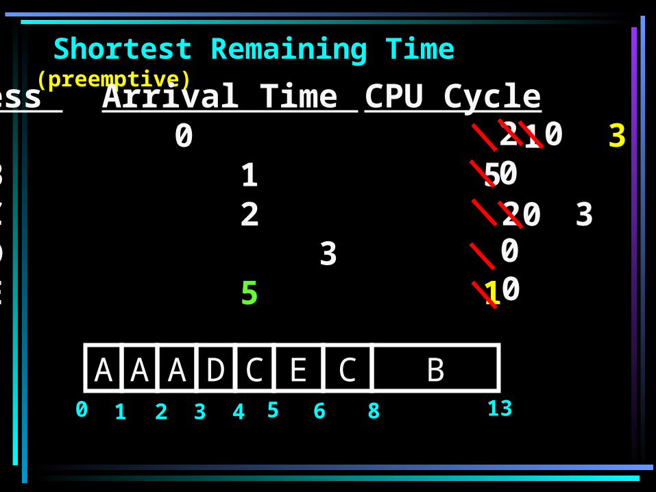
Shortest Remaining Time (preemptive)
Process Arrival Time CPU Cycle A 0 3 B 1 5 C 2 3 D 3 1 E 5 1
0 1 5 6 8
A E C2
A3
D4
C
2
020
1
0
A
0
0
B13

Shortest Remaining Time (preemptive)
Process Arrival Time CPU Cycle A 0 3 B 1 5 C 2 3 D 3 1 E 5 1
0 1 5 6 8
A E C2 3
D4
C B13

•Round Robin
•Preemptive.•Used extensively in interactive systems because it’s easy to implement. •Isn’t based on job characteristics but on a predetermined slice of time that’s given to each job.
Ensures CPU is equally shared among all active processes and isn’t monopolized by any one job.
•Time slice is called a time quantum size crucial to system performance (100 ms to 1-2 secs)
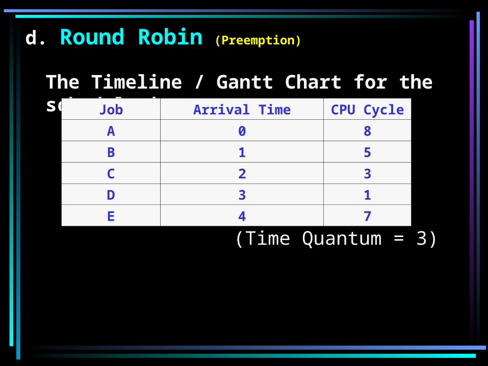
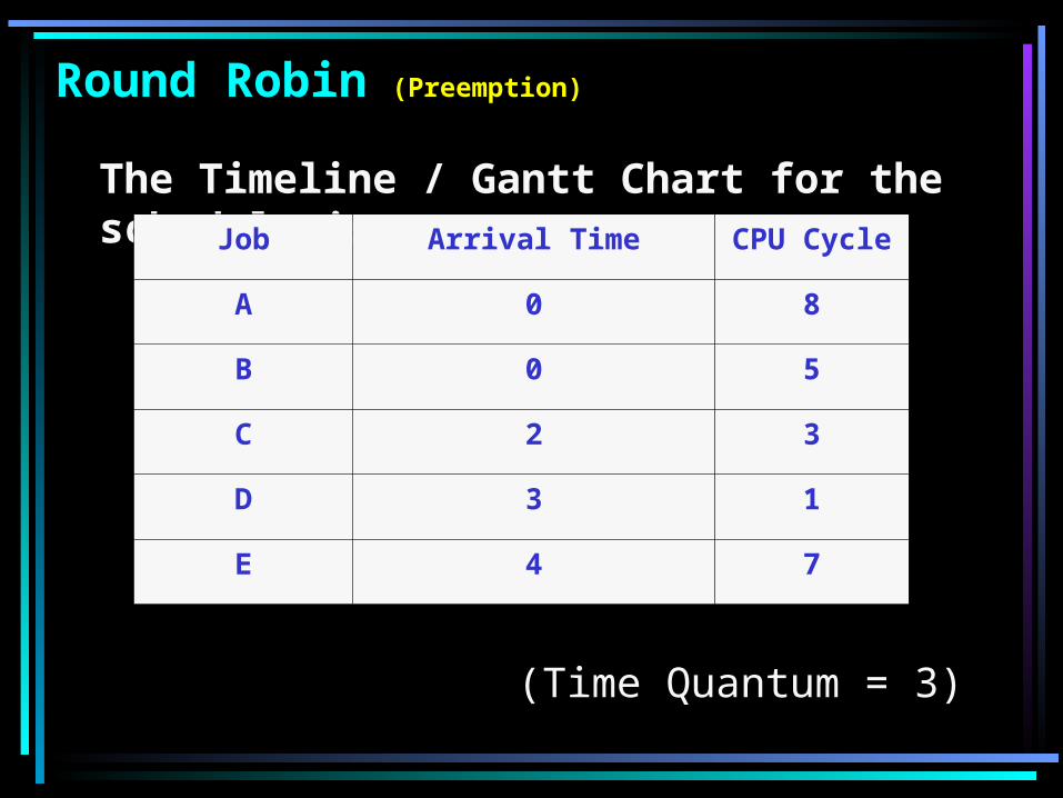
d. Round Robin (Preemption)
The Timeline / Gantt Chart for the schedule is:Job Arrival Time CPU Cycle
A 0 8
B 1 5
C 2 3
D 3 1
E 4 7
(Time Quantum = 3)
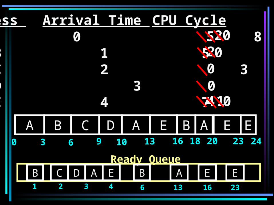
A0 3 6 9
B C D10 13
A E16
B18
A E20 23
Process Arrival Time CPU Cycle A 0 8 B 1 5 C 2 3 D 3 1 E 4 7
Ready Queue
5
B C21
D3
A
2
E4
B6
00
2
A13
4
00
E16
E23
1
E24
0
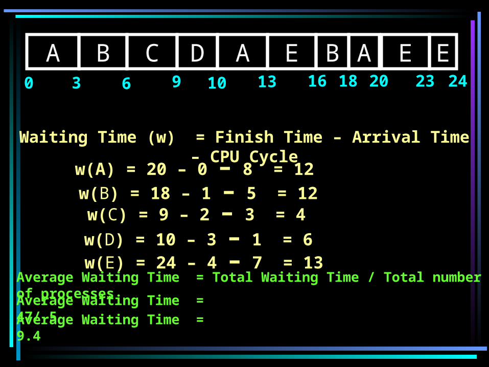
Waiting Time (w) = Finish Time – Arrival Time – CPU Cyclew(A) = 20 – 0 – 8 = 12
w(B) = 18 – 1 – 5 = 12w(C) = 9 – 2 – 3 = 4
w(D) = 10 – 3 – 1 = 6w(E) = 24 – 4 – 7 = 13
Average Waiting Time = Total Waiting Time / Total number of processes
Average Waiting Time = 47/ 5
Average Waiting Time = 9.4
A0 3 6 9
B C D10 13
A E16
B18
A E20 23
E24
A0 3 6 9
B C D10 13
A E16
B18
A E20 23
E24
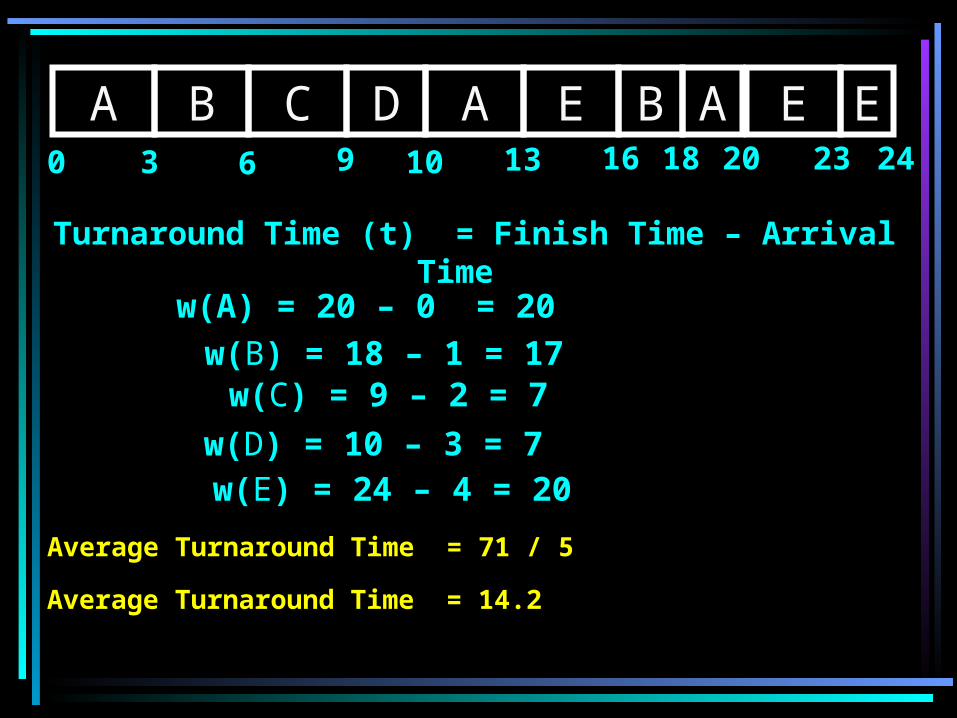
Turnaround Time (t) = Finish Time – Arrival Time
w(A) = 20 – 0 = 20
w(B) = 18 – 1 = 17w(C) = 9 – 2 = 7
w(D) = 10 – 3 = 7w(E) = 24 – 4 = 20
Average Turnaround Time = 71 / 5
Average Turnaround Time = 14.2
Round Robin (Preemption)
The Timeline / Gantt Chart for the schedule is:Job Arrival Time CPU Cycle
A 0 8
B 0 5
C 2 3
D 3 1
E 4 7
(Time Quantum = 3)

A0 3 6 9
B C D10 13
A E16
B18
A E20 23
Process Arrival Time CPU Cycle A 0 8 B 0 5 C 2 3 D 3 1 E 4 7
Ready Queue
5
B C20
D3
A
2
E4
B6
00
2
A13
4
00
E16
E23
1
E24
0

•If Job’s CPU Cycle < Time Quantum•If job’s last CPU cycle & job is finished, then all resources allocated to it are released & completed job is returned to user.•If CPU cycle was interrupted by I/O request, then info about the job is saved in its PCB & it is linked at end of the appropriate I/O queue. Later, when I/O request has been satisfied, it is returned to end of READY queue to await allocation of CPU

Round Robin (Preemption)
The Timeline / Gantt Chart for the schedule is:Job Arrival Time CPU Cycle
A 0 8
B 0 5
C 0 3
D 0 1
E 0 7
(Time Quantum = 3)

A0 3 6 9
B C D10 13
E16
A18
B21 23
Process Arrival Time CPU Cycle A 0 8 B 0 5 C 0 3 D 0 1 E 0 7
Ready QueueB C
0
D E3
B6
A13
E16
E24
A
A E
E21

•Time Slices Should Be ...•Long enough to allow 80 % of CPU cycles to run to completion.
•At least 100 times longer than time required to perform one context switch. •Flexible - depends on the system.
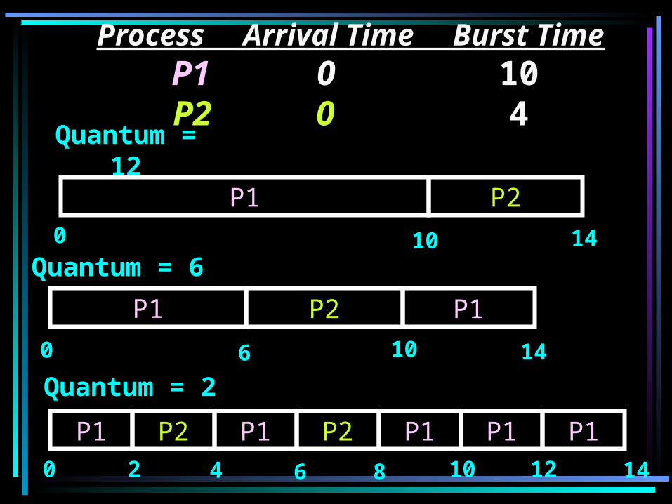
Process Arrival Time Burst Time P1 0 10P2 0 4
Quantum = 6
P1
0 6
P2
10
P1
14
Quantum = 2
P1 P2 P2P1 P1 P1
0 2 4 6 8 10 12 14
P1
100
P1
Quantum = 12
P2
14

e. Non-Preemptive Priority Process Arrival Time Burst Time Priority P1 0.0 7 9 P2 2.0 4 10 P3 2.0 1 9 P4 5.0 4 11
Assume a larger no implies a higher priority
0 7 11
P1 P4 P2 P315 16

Priority Scheduling Non-preemptive algorithm which is commonly used in batch systems.Gives preferential treatment to important jobs.Allows the program with the highest priority to be processed first and these high priority jobs are not interrupted until their CPU cycles (run times) are completed or a natural wait occurs.If two or more jobs with equal priority, then uses FCFS policy within the same priority group

f. Preemptive Priority Process Arrival Time Burst Time Priority P1 0.0 7 9 P2 2.0 4 10 P3 2.0 1 9 P4 5.0 4 11
Assume a larger no implies a higher priority
0 2 5 9 10 15 16
P1 P4P2 P2 P1 P3
5
1
0
0
0
0
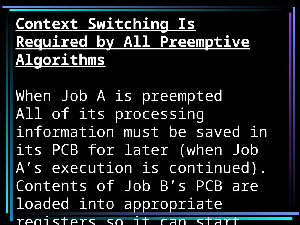
Context Switching Is Required by All Preemptive Algorithms When Job A is preemptedAll of its processing information must be saved in its PCB for later (when Job A’s execution is continued).Contents of Job B’s PCB are loaded into appropriate registers so it can start running again (context switch).
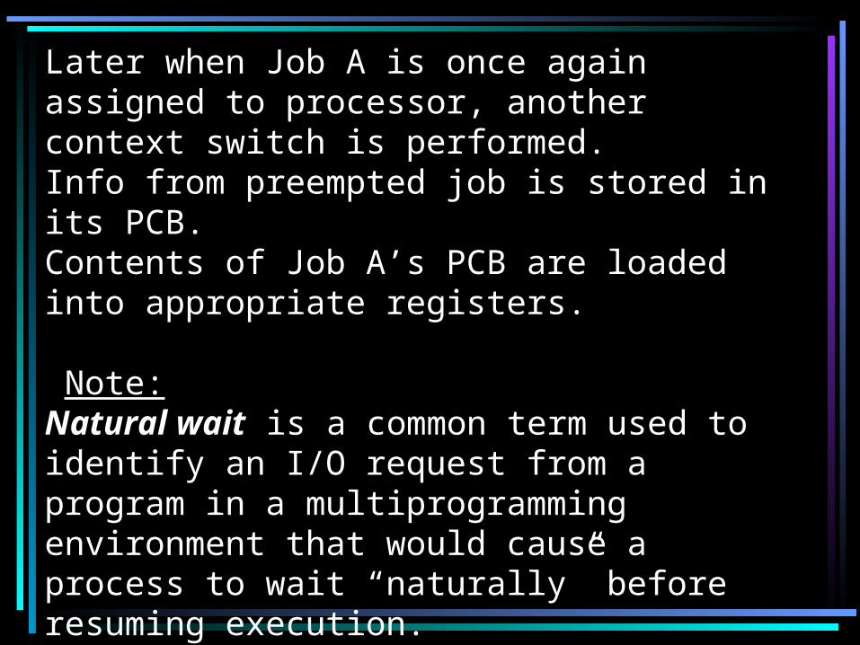
Later when Job A is once again assigned to processor, another context switch is performed.Info from preempted job is stored in its PCB.Contents of Job A’s PCB are loaded into appropriate registers. Note:Natural wait is a common term used to identify an I/O request from a program in a multiprogramming environment that would cause a process to wait “naturally” before resuming execution.

Round RobinProcess Burst Time
P1 53P2 20P3 68P4 24
Eg. Time Quantum = 20ms and Context Switch =2ms
0 20 64 66 86
P4P3P122
P242 44
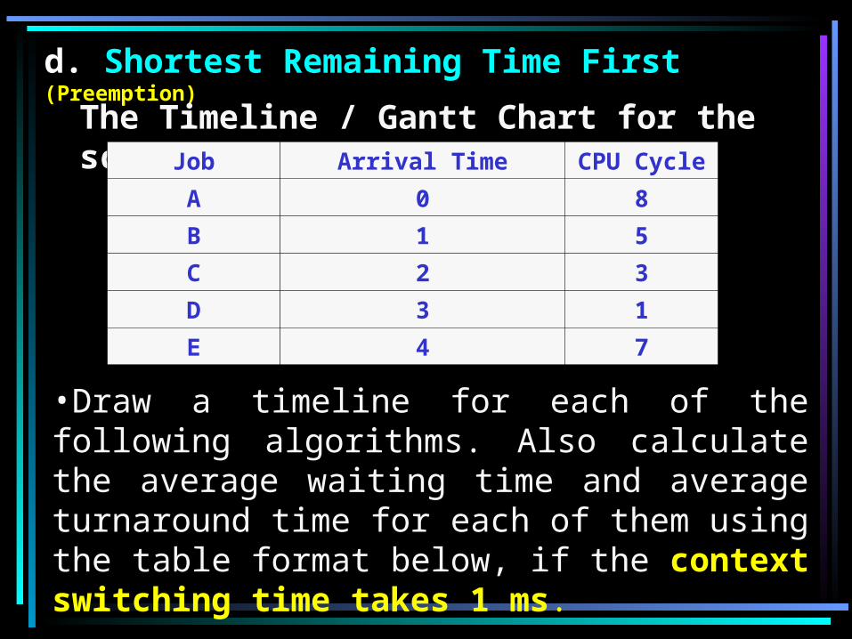
d. Shortest Remaining Time First (Preemption)
The Timeline / Gantt Chart for the schedule is:Job Arrival Time CPU Cycle
A 0 8
B 1 5
C 2 3
D 3 1
E 4 7
•Draw a timeline for each of the following algorithms. Also calculate the average waiting time and average turnaround time for each of them using the table format below, if the context switching time takes 1 ms.

d. Round Robin (Preemption)
The Timeline / Gantt Chart for the schedule is:Job Arrival Time CPU Cycle
A 0 8
B 1 5
C 2 3
D 3 1
E 4 7
(Time Quantum = 3)
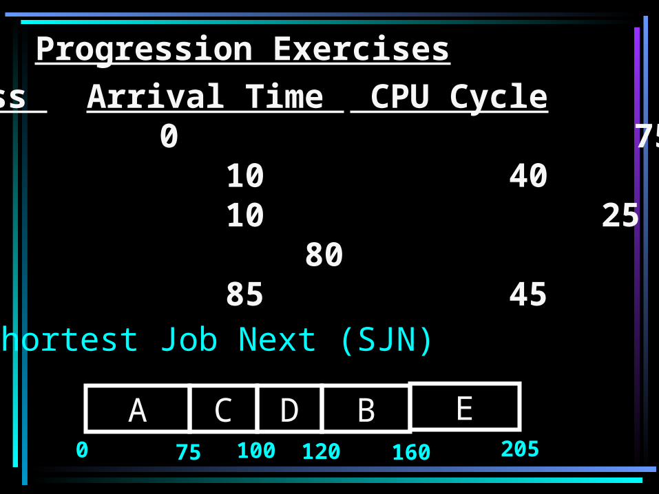
Progression ExercisesProcess Arrival Time CPU Cycle A 0 75 B 10 40 C 10 25 D 80 20 E 85 45
0 100 120 160
A D B75
C E205
Shortest Job Next (SJN)

Shortest Remaining Time First (preemptive)
Process Arrival Time CPU Cycle A 0 75 B 10 40 C 10 25 D 80 20 E 85 45
0 10 75 80 85
A B AC205
D35
E100
65
00
60
15
D
0
145
0
A
0
Related Documents