10-1 © 2007 Pearson Education Chapter 10 Managing Economies of Scale in the Supply Chain: Cycle Inventory Supply Chain Management (3rd Edition)

Welcome message from author
This document is posted to help you gain knowledge. Please leave a comment to let me know what you think about it! Share it to your friends and learn new things together.
Transcript
10-1© 2007 Pearson Education
Chapter 10Managing Economies of Scale in the
Supply Chain: Cycle Inventory
Supply Chain Management(3rd Edition)
10-2© 2007 Pearson Education
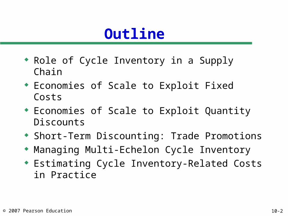
Outline
Role of Cycle Inventory in a Supply Chain Economies of Scale to Exploit Fixed Costs Economies of Scale to Exploit Quantity Discounts Short-Term Discounting: Trade Promotions Managing Multi-Echelon Cycle Inventory Estimating Cycle Inventory-Related Costs in
Practice
10-3© 2007 Pearson Education
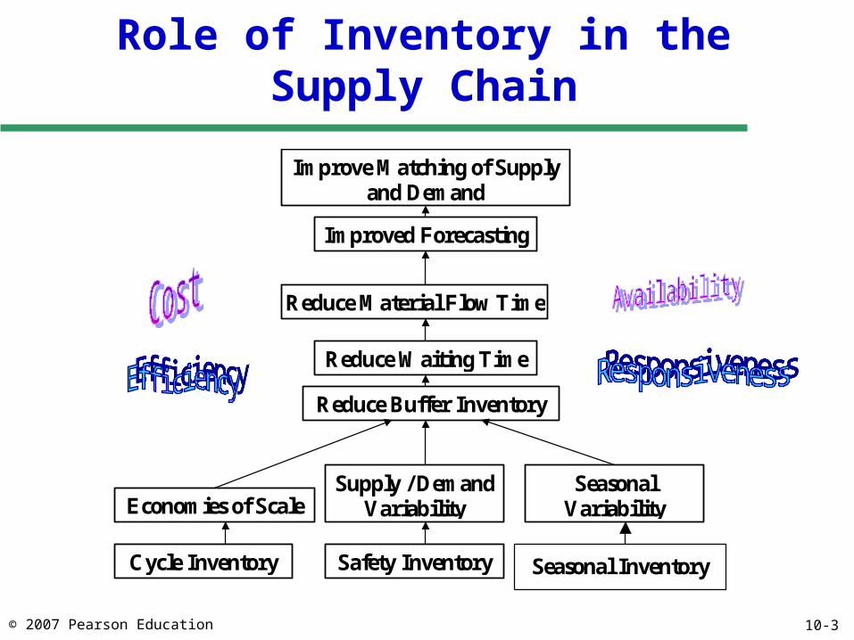
Role of Inventory in the Supply Chain
Improve Matching of Supplyand Demand
Improved Forecasting
Reduce Material Flow Time
Reduce Waiting Time
Reduce Buffer Inventory
Economies of ScaleSupply / Demand
VariabilitySeasonal
Variability
Cycle Inventory Safety InventoryFigure Error! No text of
Seasonal Inventory
10-4© 2007 Pearson Education
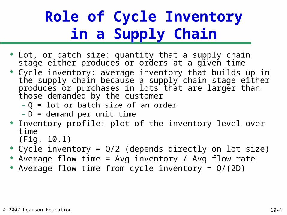
Role of Cycle Inventoryin a Supply Chain
Lot, or batch size: quantity that a supply chain stage either produces or orders at a given time
Cycle inventory: average inventory that builds up in the supply chain because a supply chain stage either produces or purchases in lots that are larger than those demanded by the customer– Q = lot or batch size of an order– D = demand per unit time
Inventory profile: plot of the inventory level over time (Fig. 10.1)
Cycle inventory = Q/2 (depends directly on lot size) Average flow time = Avg inventory / Avg flow rate Average flow time from cycle inventory = Q/(2D)
10-5© 2007 Pearson Education
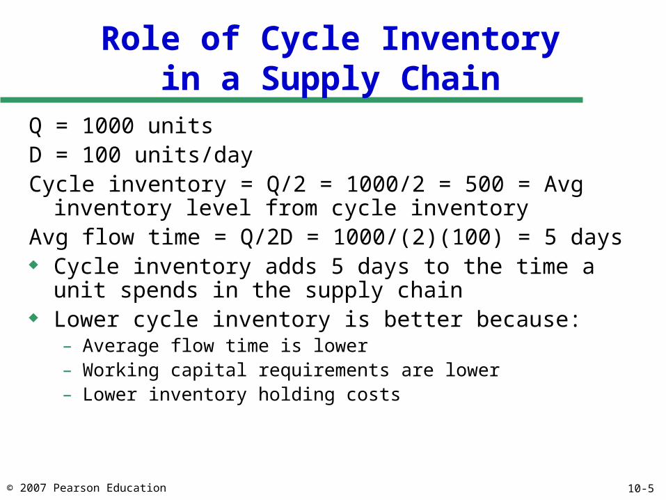
Role of Cycle Inventoryin a Supply Chain
Q = 1000 unitsD = 100 units/dayCycle inventory = Q/2 = 1000/2 = 500 = Avg inventory level from
cycle inventoryAvg flow time = Q/2D = 1000/(2)(100) = 5 days Cycle inventory adds 5 days to the time a unit spends in the
supply chain Lower cycle inventory is better because:
– Average flow time is lower– Working capital requirements are lower– Lower inventory holding costs
10-6© 2007 Pearson Education
Role of Cycle Inventoryin a Supply Chain
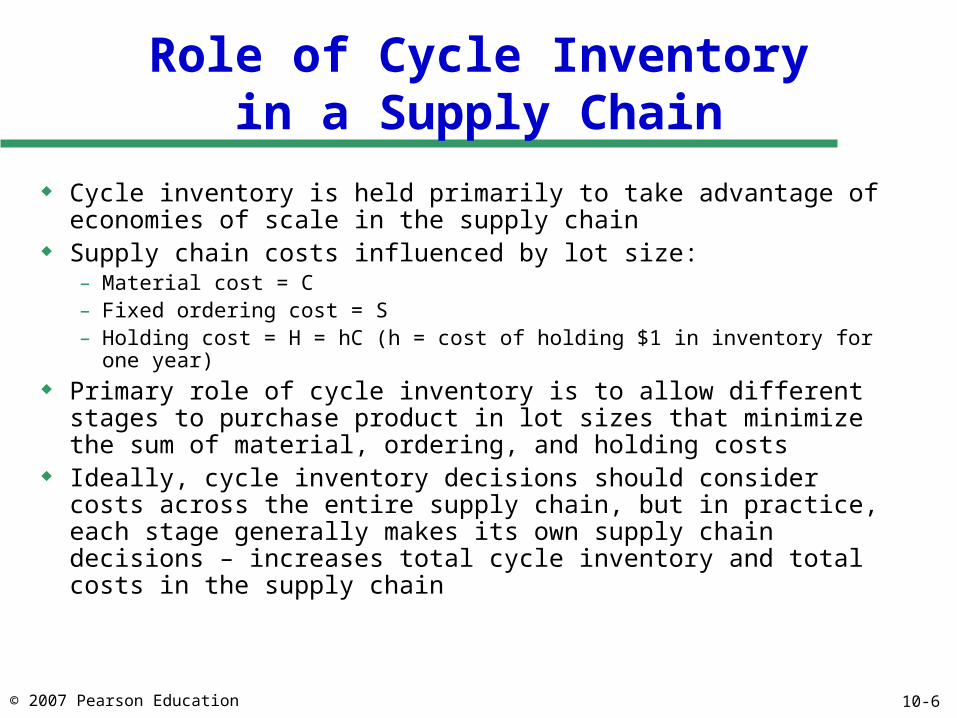
Cycle inventory is held primarily to take advantage of economies of scale in the supply chain
Supply chain costs influenced by lot size:– Material cost = C– Fixed ordering cost = S– Holding cost = H = hC (h = cost of holding $1 in inventory for one year)
Primary role of cycle inventory is to allow different stages to purchase product in lot sizes that minimize the sum of material, ordering, and holding costs
Ideally, cycle inventory decisions should consider costs across the entire supply chain, but in practice, each stage generally makes its own supply chain decisions – increases total cycle inventory and total costs in the supply chain
10-7© 2007 Pearson Education
Economies of Scaleto Exploit Fixed Costs
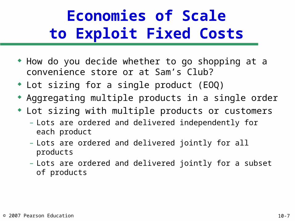
How do you decide whether to go shopping at a convenience store or at Sam’s Club?
Lot sizing for a single product (EOQ) Aggregating multiple products in a single order Lot sizing with multiple products or customers
– Lots are ordered and delivered independently for each product
– Lots are ordered and delivered jointly for all products
– Lots are ordered and delivered jointly for a subset of products
10-8© 2007 Pearson Education
Economies of Scaleto Exploit Fixed Costs
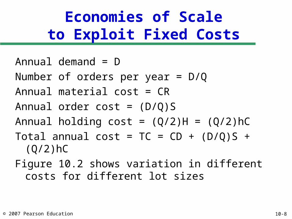
Annual demand = D
Number of orders per year = D/Q
Annual material cost = CR
Annual order cost = (D/Q)S
Annual holding cost = (Q/2)H = (Q/2)hC
Total annual cost = TC = CD + (D/Q)S + (Q/2)hC
Figure 10.2 shows variation in different costs for different lot sizes
10-9© 2007 Pearson Education
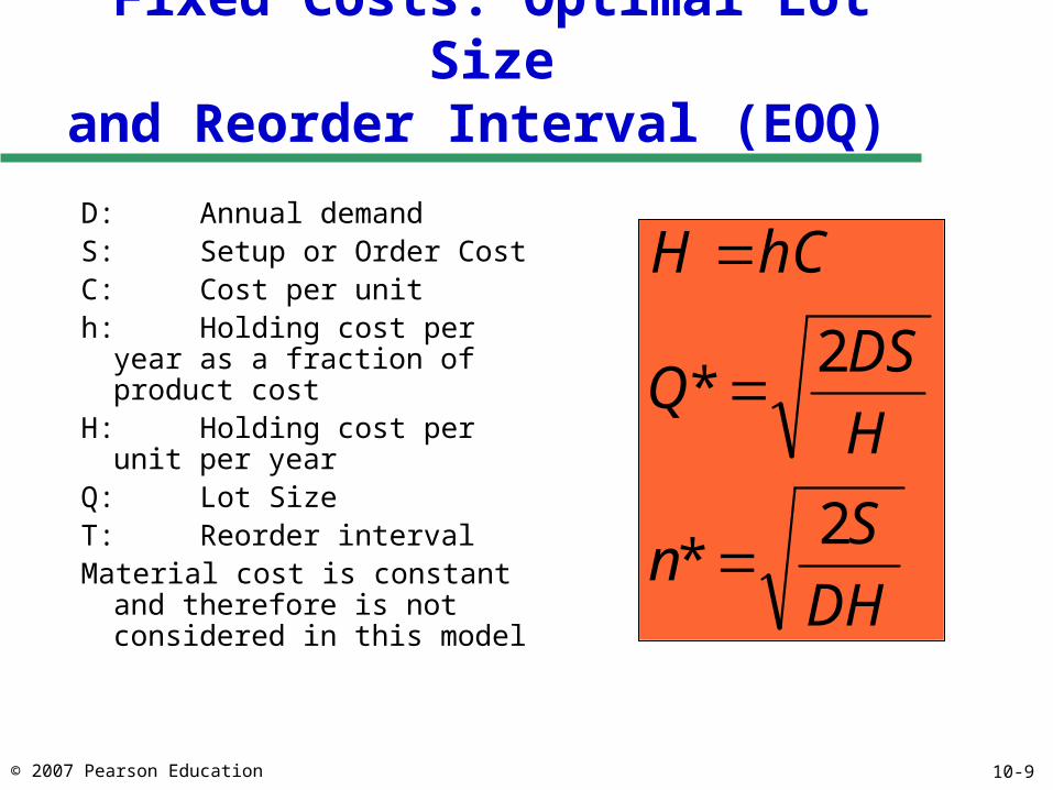
Fixed Costs: Optimal Lot Sizeand Reorder Interval (EOQ)
D: Annual demand S: Setup or Order CostC: Cost per unith: Holding cost per year as a
fraction of product costH: Holding cost per unit per yearQ: Lot SizeT: Reorder intervalMaterial cost is constant and
therefore is not considered in this model
DH
Sn
H
DSQ
hCH
2*
2*
10-10© 2007 Pearson Education
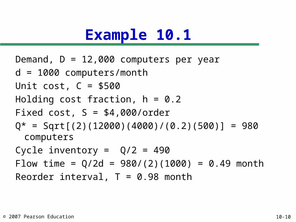
Example 10.1
Demand, D = 12,000 computers per year
d = 1000 computers/month
Unit cost, C = $500
Holding cost fraction, h = 0.2
Fixed cost, S = $4,000/order
Q* = Sqrt[(2)(12000)(4000)/(0.2)(500)] = 980 computers
Cycle inventory = Q/2 = 490
Flow time = Q/2d = 980/(2)(1000) = 0.49 month
Reorder interval, T = 0.98 month
10-11© 2007 Pearson Education
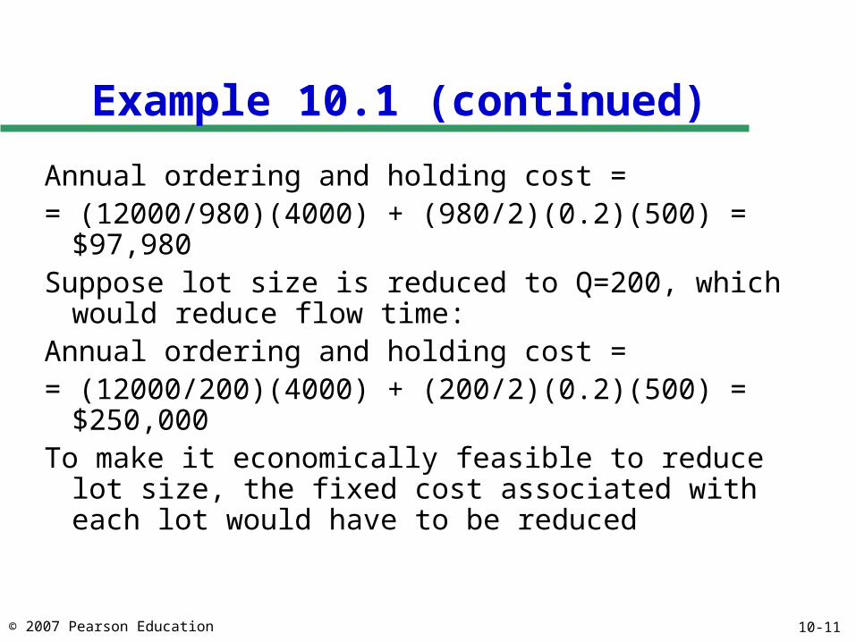
Example 10.1 (continued)
Annual ordering and holding cost = = (12000/980)(4000) + (980/2)(0.2)(500) = $97,980Suppose lot size is reduced to Q=200, which would
reduce flow time:Annual ordering and holding cost = = (12000/200)(4000) + (200/2)(0.2)(500) = $250,000To make it economically feasible to reduce lot size, the
fixed cost associated with each lot would have to be reduced
10-12© 2007 Pearson Education
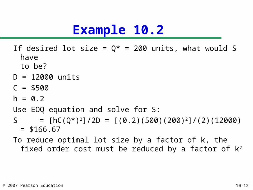
Example 10.2
If desired lot size = Q* = 200 units, what would S haveto be?
D = 12000 units
C = $500
h = 0.2
Use EOQ equation and solve for S:
S = [hC(Q*)2]/2D = [(0.2)(500)(200)2]/(2)(12000) = $166.67
To reduce optimal lot size by a factor of k, the fixed order cost must be reduced by a factor of k2
10-13© 2007 Pearson Education
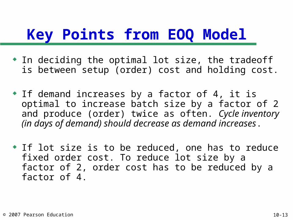
Key Points from EOQ Model
In deciding the optimal lot size, the tradeoff is between setup (order) cost and holding cost.
If demand increases by a factor of 4, it is optimal to increase batch size by a factor of 2 and produce (order) twice as often. Cycle inventory (in days of demand) should decrease as demand increases.
If lot size is to be reduced, one has to reduce fixed order cost. To reduce lot size by a factor of 2, order cost has to be reduced by a factor of 4.
10-14© 2007 Pearson Education
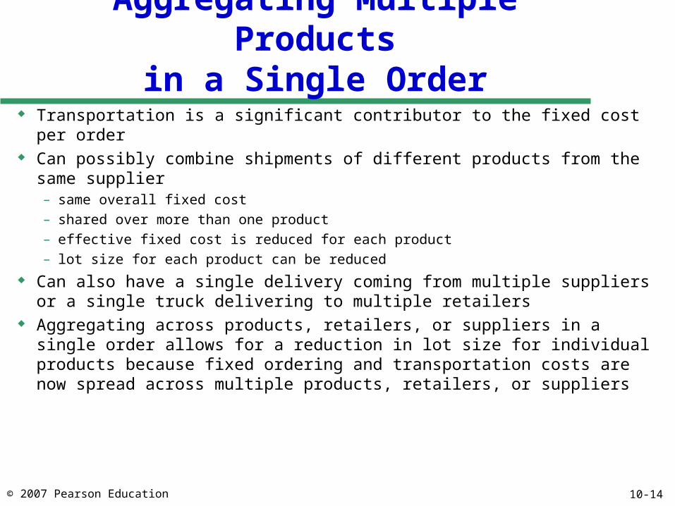
Aggregating Multiple Productsin a Single Order
Transportation is a significant contributor to the fixed cost per order Can possibly combine shipments of different products from the same supplier
– same overall fixed cost– shared over more than one product– effective fixed cost is reduced for each product– lot size for each product can be reduced
Can also have a single delivery coming from multiple suppliers or a single truck delivering to multiple retailers
Aggregating across products, retailers, or suppliers in a single order allows for a reduction in lot size for individual products because fixed ordering and transportation costs are now spread across multiple products, retailers, or suppliers
10-15© 2007 Pearson Education
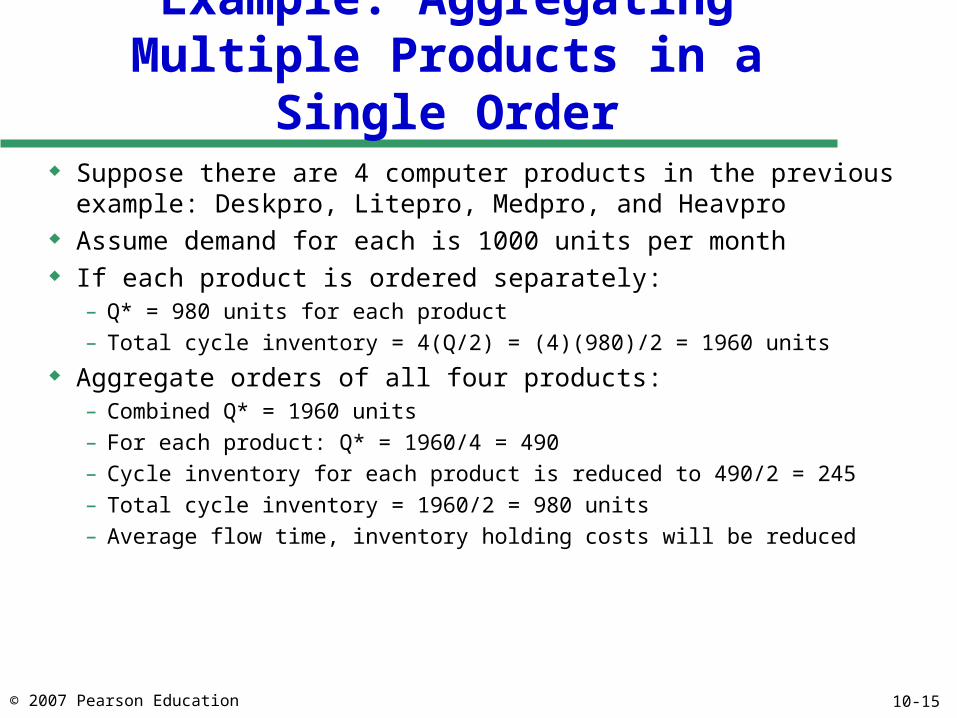
Example: Aggregating Multiple Products in a Single Order
Suppose there are 4 computer products in the previous example: Deskpro, Litepro, Medpro, and Heavpro
Assume demand for each is 1000 units per month If each product is ordered separately:
– Q* = 980 units for each product– Total cycle inventory = 4(Q/2) = (4)(980)/2 = 1960 units
Aggregate orders of all four products:– Combined Q* = 1960 units– For each product: Q* = 1960/4 = 490– Cycle inventory for each product is reduced to 490/2 = 245– Total cycle inventory = 1960/2 = 980 units– Average flow time, inventory holding costs will be reduced
10-16© 2007 Pearson Education
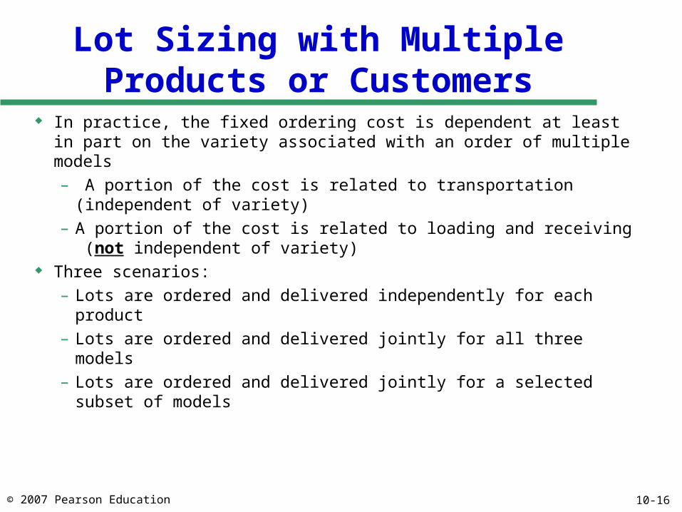
Lot Sizing with MultipleProducts or Customers
In practice, the fixed ordering cost is dependent at least in part on the variety associated with an order of multiple models– A portion of the cost is related to transportation (independent of
variety)– A portion of the cost is related to loading and receiving (not
independent of variety) Three scenarios:
– Lots are ordered and delivered independently for each product– Lots are ordered and delivered jointly for all three models– Lots are ordered and delivered jointly for a selected subset of
models
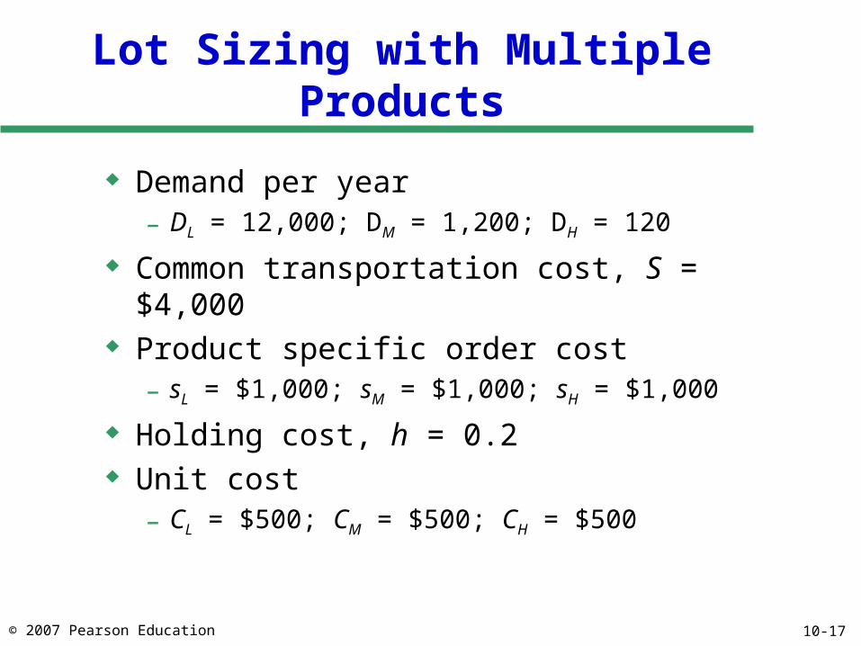
10-17© 2007 Pearson Education
Lot Sizing with Multiple Products
Demand per year– DL = 12,000; DM = 1,200; DH = 120
Common transportation cost, S = $4,000 Product specific order cost
– sL = $1,000; sM = $1,000; sH = $1,000
Holding cost, h = 0.2 Unit cost
– CL = $500; CM = $500; CH = $500
10-18© 2007 Pearson Education
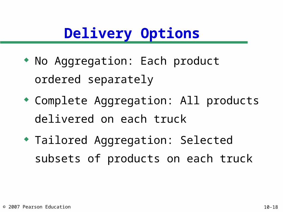
Delivery Options
No Aggregation: Each product ordered separately
Complete Aggregation: All products delivered on
each truck
Tailored Aggregation: Selected subsets of products
on each truck
10-19© 2007 Pearson Education
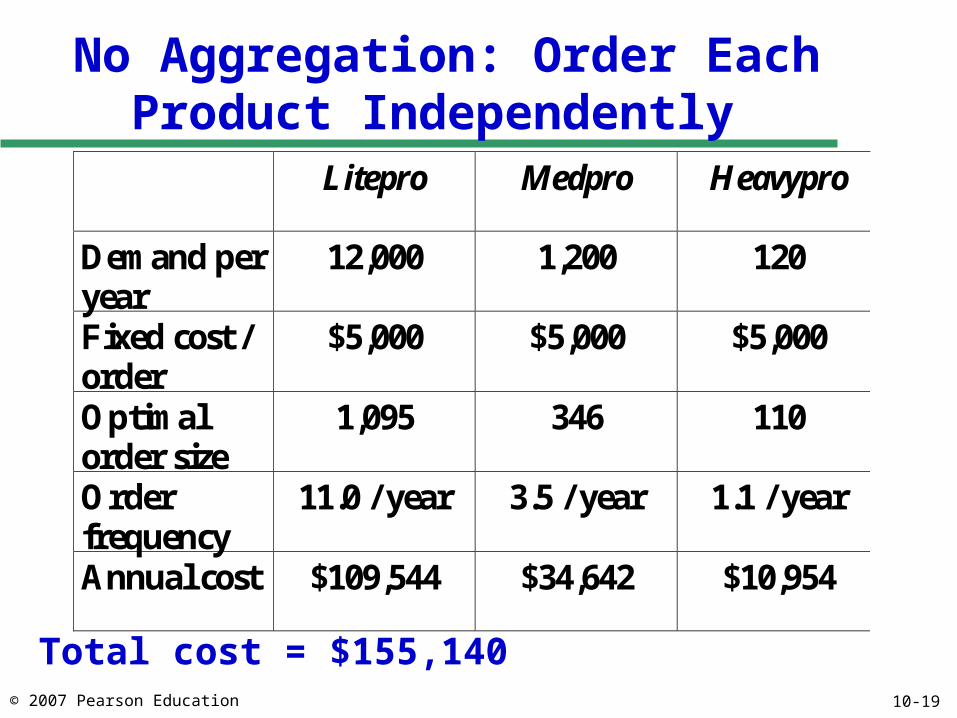
No Aggregation: Order Each Product Independently
Litepro Medpro Heavypro
Demand per year
12,000 1,200 120
Fixed cost / order
$5,000 $5,000 $5,000
Optimal order size
1,095 346 110
Order frequency
11.0 / year 3.5 / year 1.1 / year
Annual cost $109,544 $34,642 $10,954
Total cost = $155,140
10-20© 2007 Pearson Education
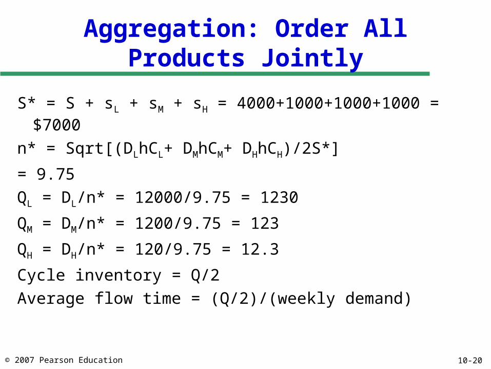
Aggregation: Order AllProducts Jointly
S* = S + sL + sM + sH = 4000+1000+1000+1000 = $7000
n* = Sqrt[(DLhCL+ DMhCM+ DHhCH)/2S*]
= 9.75
QL = DL/n* = 12000/9.75 = 1230
QM = DM/n* = 1200/9.75 = 123
QH = DH/n* = 120/9.75 = 12.3
Cycle inventory = Q/2
Average flow time = (Q/2)/(weekly demand)
10-21© 2007 Pearson Education
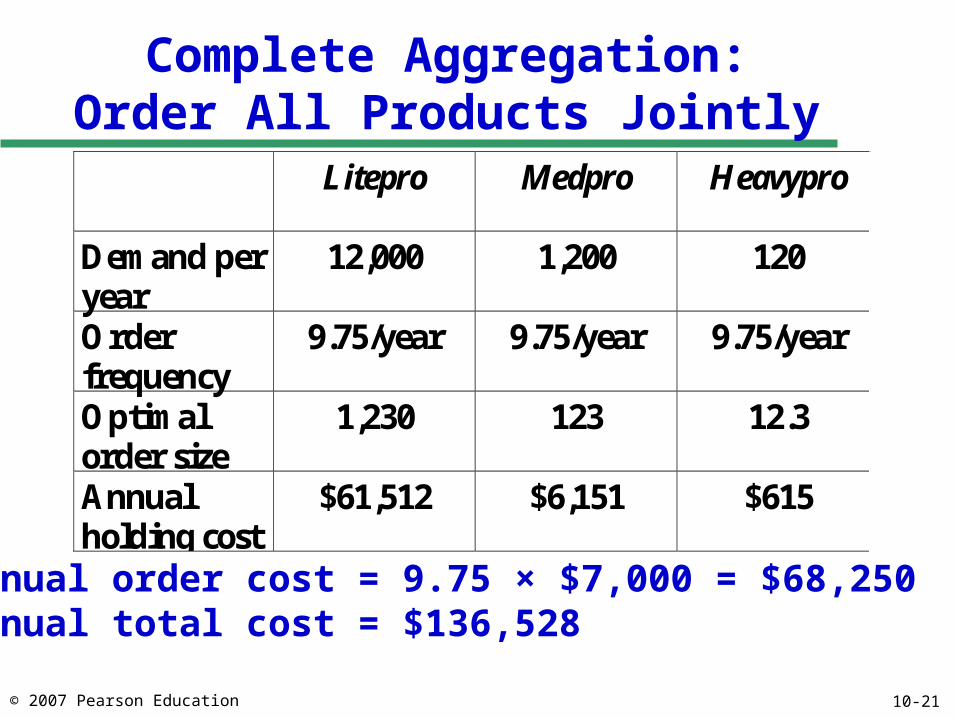
Complete Aggregation:Order All Products Jointly
Litepro Medpro Heavypro
Demand peryear
12,000 1,200 120
Orderfrequency
9.75/year 9.75/year 9.75/year
Optimalorder size
1,230 123 12.3
Annualholding cost
$61,512 $6,151 $615
Annual order cost = 9.75 × $7,000 = $68,250Annual total cost = $136,528
10-22© 2007 Pearson Education
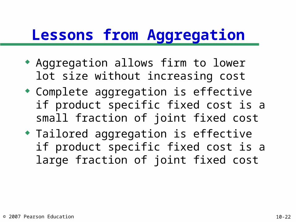
Lessons from Aggregation
Aggregation allows firm to lower lot size without increasing cost
Complete aggregation is effective if product specific fixed cost is a small fraction of joint fixed cost
Tailored aggregation is effective if product specific fixed cost is a large fraction of joint fixed cost
10-23© 2007 Pearson Education
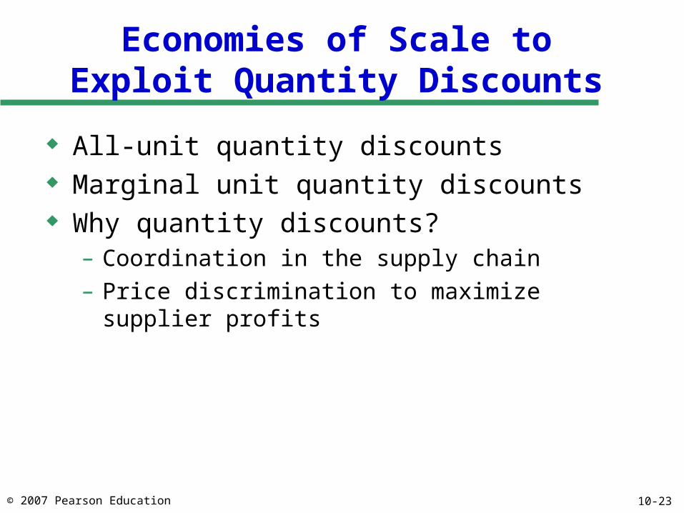
Economies of Scale toExploit Quantity Discounts
All-unit quantity discounts Marginal unit quantity discounts Why quantity discounts?
– Coordination in the supply chain
– Price discrimination to maximize supplier profits
10-24© 2007 Pearson Education
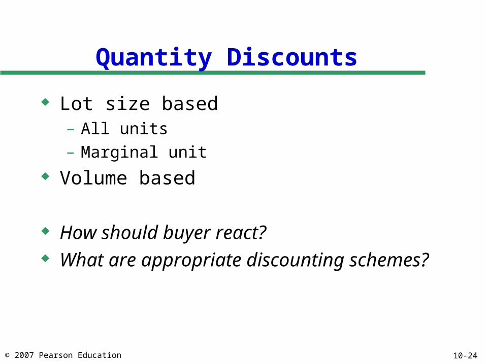
Quantity Discounts
Lot size based– All units
– Marginal unit
Volume based
How should buyer react? What are appropriate discounting schemes?
10-25© 2007 Pearson Education
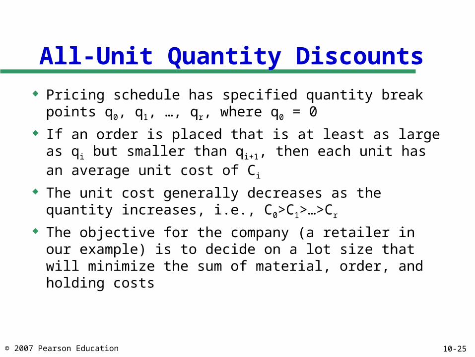
All-Unit Quantity Discounts
Pricing schedule has specified quantity break points q0, q1, …, qr, where q0 = 0
If an order is placed that is at least as large as qi but smaller than qi+1, then each unit has an average unit cost of Ci
The unit cost generally decreases as the quantity increases, i.e., C0>C1>…>Cr
The objective for the company (a retailer in our example) is to decide on a lot size that will minimize the sum of material, order, and holding costs
10-26© 2007 Pearson Education
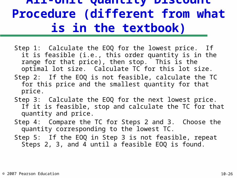
All-Unit Quantity Discount Procedure (different from what is in the textbook)
Step 1: Calculate the EOQ for the lowest price. If it is feasible (i.e., this order quantity is in the range for that price), then stop. This is the optimal lot size. Calculate TC for this lot size.
Step 2: If the EOQ is not feasible, calculate the TC for this price and the smallest quantity for that price.
Step 3: Calculate the EOQ for the next lowest price. If it is feasible, stop and calculate the TC for that quantity and price.
Step 4: Compare the TC for Steps 2 and 3. Choose the quantity corresponding to the lowest TC.
Step 5: If the EOQ in Step 3 is not feasible, repeat Steps 2, 3, and 4 until a feasible EOQ is found.
10-27© 2007 Pearson Education
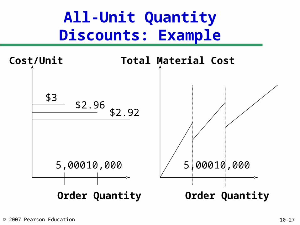
All-Unit Quantity Discounts: Example
Cost/Unit
$3$2.96
$2.92
Order Quantity
5,000 10,000
Order Quantity
5,000 10,000
Total Material Cost
10-28© 2007 Pearson Education
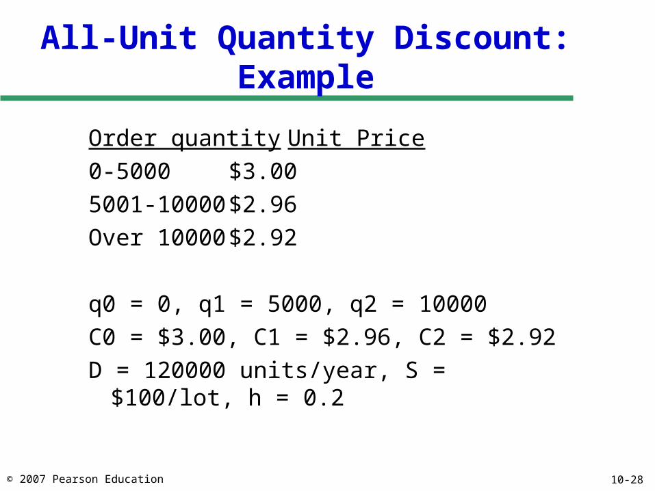
All-Unit Quantity Discount: Example
Order quantity Unit Price
0-5000 $3.00
5001-10000 $2.96
Over 10000 $2.92
q0 = 0, q1 = 5000, q2 = 10000
C0 = $3.00, C1 = $2.96, C2 = $2.92
D = 120000 units/year, S = $100/lot, h = 0.2
10-29© 2007 Pearson Education
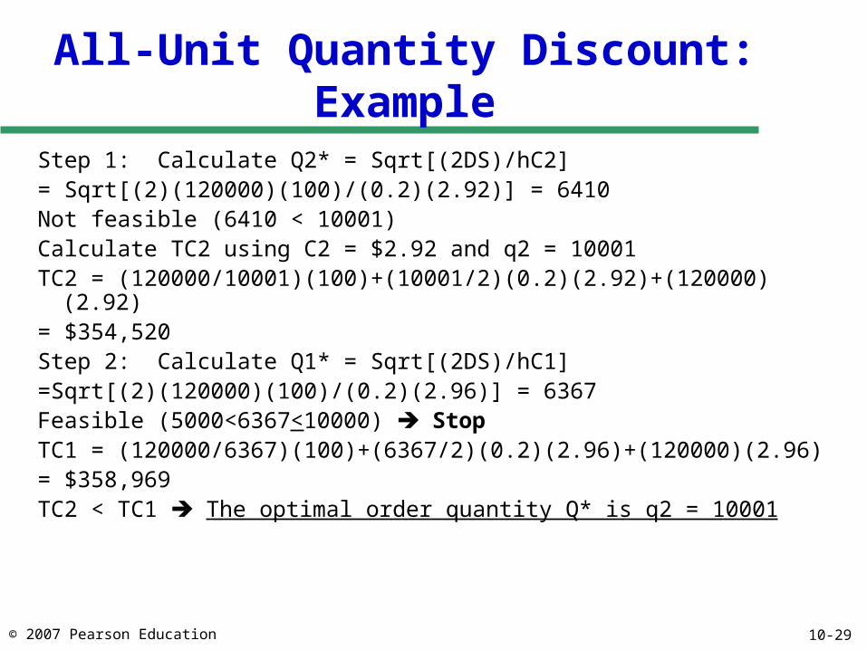
All-Unit Quantity Discount: Example
Step 1: Calculate Q2* = Sqrt[(2DS)/hC2] = Sqrt[(2)(120000)(100)/(0.2)(2.92)] = 6410Not feasible (6410 < 10001)Calculate TC2 using C2 = $2.92 and q2 = 10001TC2 = (120000/10001)(100)+(10001/2)(0.2)(2.92)+(120000)(2.92)= $354,520Step 2: Calculate Q1* = Sqrt[(2DS)/hC1]=Sqrt[(2)(120000)(100)/(0.2)(2.96)] = 6367Feasible (5000<6367<10000) StopTC1 = (120000/6367)(100)+(6367/2)(0.2)(2.96)+(120000)(2.96)= $358,969TC2 < TC1 The optimal order quantity Q* is q2 = 10001
10-30© 2007 Pearson Education
All-Unit Quantity Discounts
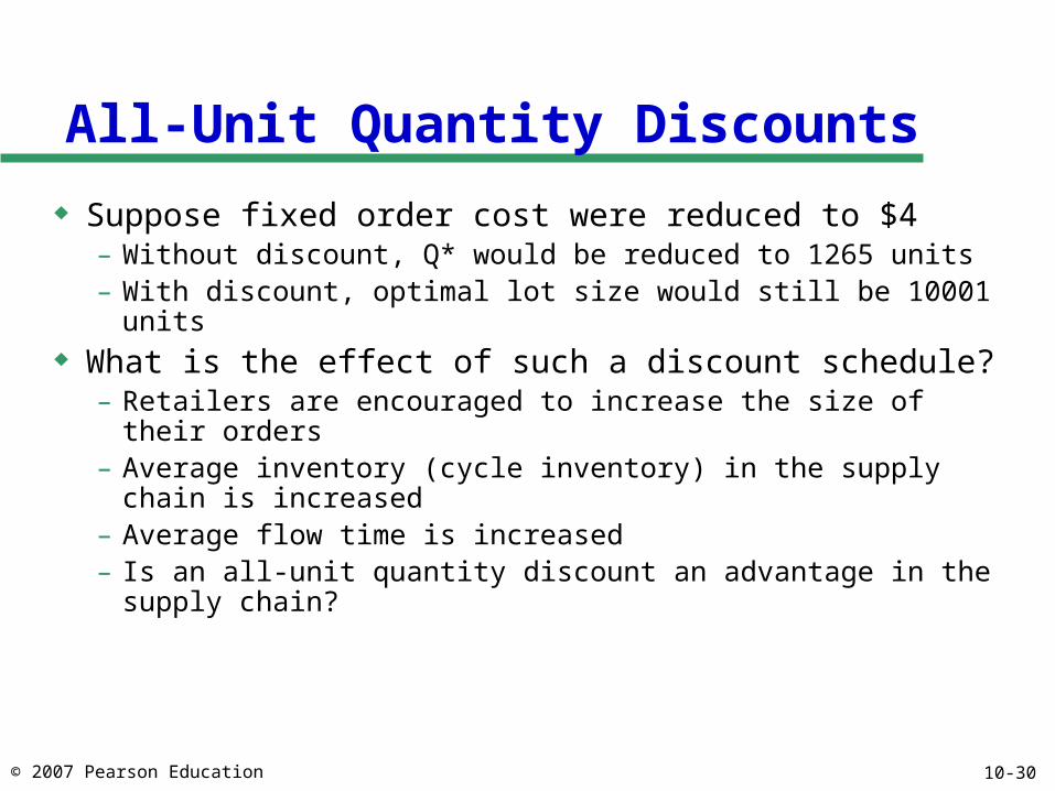
Suppose fixed order cost were reduced to $4– Without discount, Q* would be reduced to 1265 units– With discount, optimal lot size would still be 10001 units
What is the effect of such a discount schedule?– Retailers are encouraged to increase the size of their orders– Average inventory (cycle inventory) in the supply chain is
increased– Average flow time is increased– Is an all-unit quantity discount an advantage in the supply
chain?
10-31© 2007 Pearson Education
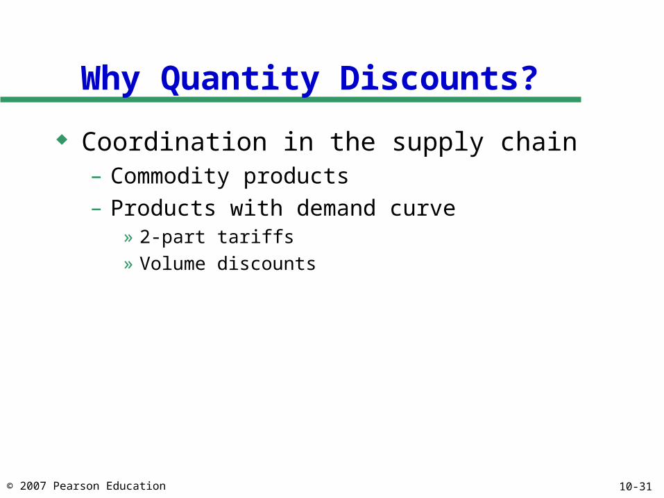
Why Quantity Discounts?
Coordination in the supply chain– Commodity products
– Products with demand curve» 2-part tariffs
» Volume discounts
10-32© 2007 Pearson Education
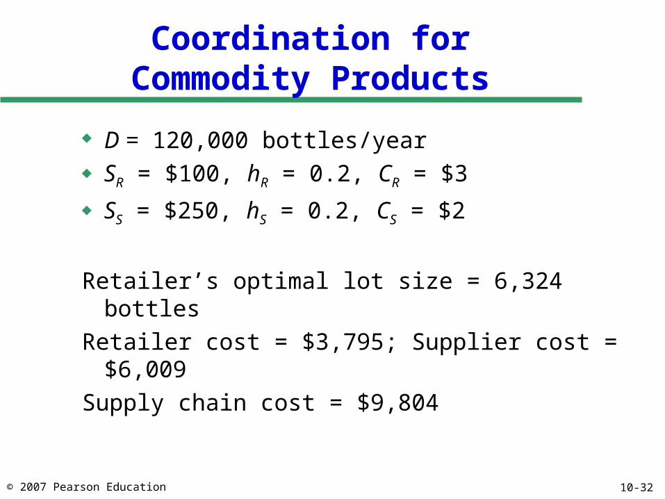
Coordination forCommodity Products
D = 120,000 bottles/year SR = $100, hR = 0.2, CR = $3
SS = $250, hS = 0.2, CS = $2
Retailer’s optimal lot size = 6,324 bottles
Retailer cost = $3,795; Supplier cost = $6,009
Supply chain cost = $9,804
10-33© 2007 Pearson Education
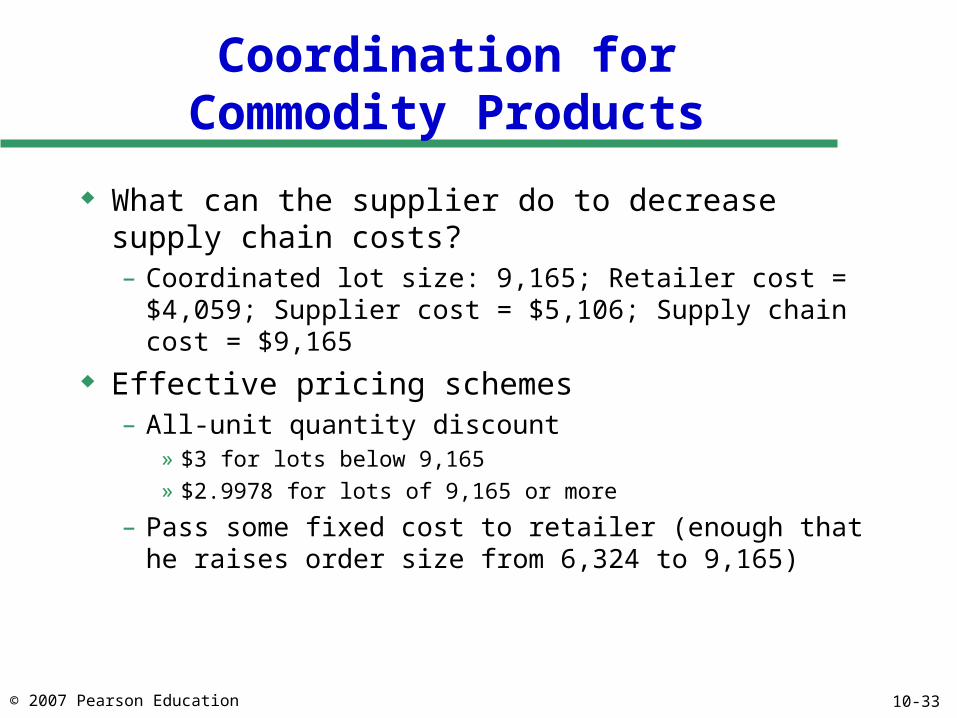
Coordination forCommodity Products
What can the supplier do to decrease supply chain costs?– Coordinated lot size: 9,165; Retailer cost = $4,059;
Supplier cost = $5,106; Supply chain cost = $9,165
Effective pricing schemes– All-unit quantity discount
» $3 for lots below 9,165
» $2.9978 for lots of 9,165 or more
– Pass some fixed cost to retailer (enough that he raises order size from 6,324 to 9,165)
10-34© 2007 Pearson Education
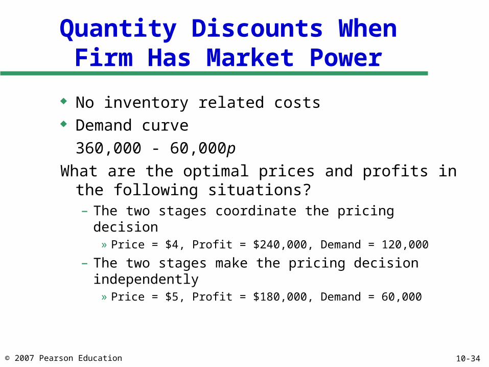
Quantity Discounts WhenFirm Has Market Power
No inventory related costs Demand curve
360,000 - 60,000p
What are the optimal prices and profits in the following situations?– The two stages coordinate the pricing decision
» Price = $4, Profit = $240,000, Demand = 120,000
– The two stages make the pricing decision independently» Price = $5, Profit = $180,000, Demand = 60,000
10-35© 2007 Pearson Education
Two-Part Tariffs andVolume Discounts
Design a two-part tariff that achieves the coordinated solution
Design a volume discount scheme that achieves the coordinated solution
Impact of inventory costs– Pass on some fixed costs with above pricing
10-36© 2007 Pearson Education
Lessons from Discounting Schemes
Lot size based discounts increase lot size and cycle inventory in the supply chain
Lot size based discounts are justified to achieve coordination for commodity products
Volume based discounts with some fixed cost passed on to retailer are more effective in general– Volume based discounts are better over rolling horizon
10-37© 2007 Pearson Education
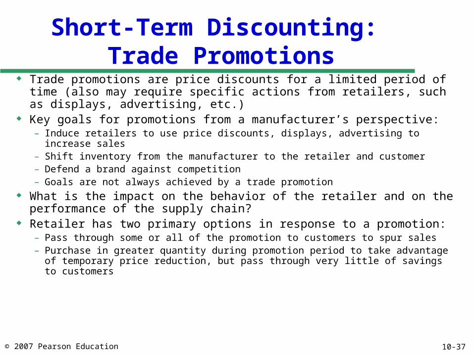
Short-Term Discounting: Trade Promotions
Trade promotions are price discounts for a limited period of time (also may require specific actions from retailers, such as displays, advertising, etc.)
Key goals for promotions from a manufacturer’s perspective:– Induce retailers to use price discounts, displays, advertising to increase sales– Shift inventory from the manufacturer to the retailer and customer– Defend a brand against competition– Goals are not always achieved by a trade promotion
What is the impact on the behavior of the retailer and on the performance of the supply chain?
Retailer has two primary options in response to a promotion:– Pass through some or all of the promotion to customers to spur sales– Purchase in greater quantity during promotion period to take advantage of temporary
price reduction, but pass through very little of savings to customers
10-38© 2007 Pearson Education
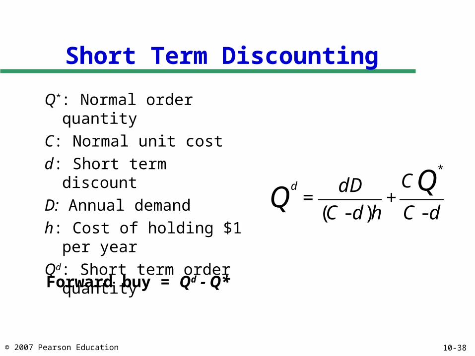
Short Term Discounting
Q*: Normal order quantity
C: Normal unit cost
d: Short term discount
D: Annual demand
h: Cost of holding $1 per year
Qd: Short term order quantity dC
C
hdC
dD QQ
d
-+
)-(=
*
Forward buy = Qd - Q*
10-39© 2007 Pearson Education
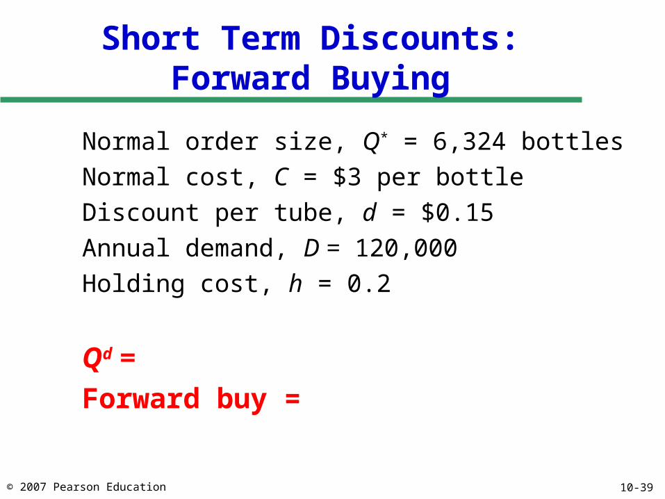
Short Term Discounts:Forward Buying
Normal order size, Q* = 6,324 bottles
Normal cost, C = $3 per bottle
Discount per tube, d = $0.15
Annual demand, D = 120,000
Holding cost, h = 0.2
Qd =
Forward buy =
10-40© 2007 Pearson Education
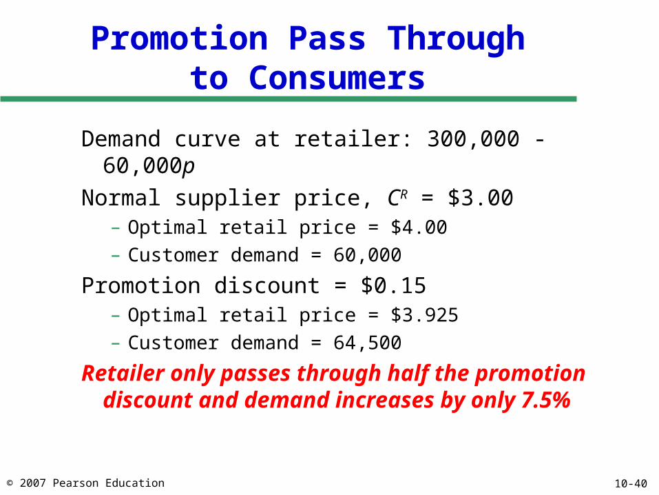
Promotion Pass Throughto Consumers
Demand curve at retailer: 300,000 - 60,000p
Normal supplier price, CR = $3.00– Optimal retail price = $4.00
– Customer demand = 60,000
Promotion discount = $0.15– Optimal retail price = $3.925
– Customer demand = 64,500
Retailer only passes through half the promotion discount and demand increases by only 7.5%
10-41© 2007 Pearson Education
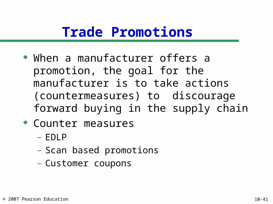
Trade Promotions
When a manufacturer offers a promotion, the goal for the manufacturer is to take actions (countermeasures) to discourage forward buying in the supply chain
Counter measures– EDLP
– Scan based promotions
– Customer coupons
10-42© 2007 Pearson Education
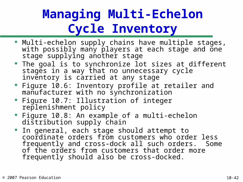
Managing Multi-EchelonCycle Inventory
Multi-echelon supply chains have multiple stages, with possibly many players at each stage and one stage supplying another stage
The goal is to synchronize lot sizes at different stages in a way that no unnecessary cycle inventory is carried at any stage
Figure 10.6: Inventory profile at retailer and manufacturer with no synchronization
Figure 10.7: Illustration of integer replenishment policy Figure 10.8: An example of a multi-echelon distribution
supply chain In general, each stage should attempt to coordinate orders
from customers who order less frequently and cross-dock all such orders. Some of the orders from customers that order more frequently should also be cross-docked.
10-43© 2007 Pearson Education
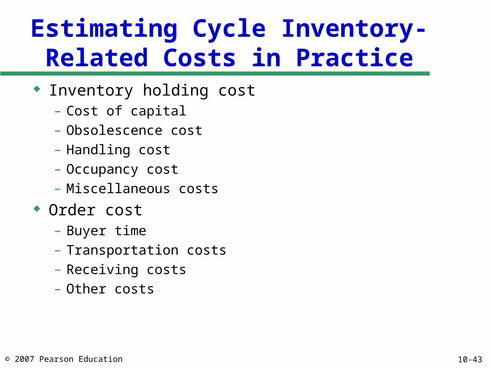
Estimating Cycle Inventory-Related Costs in Practice
Inventory holding cost– Cost of capital– Obsolescence cost– Handling cost– Occupancy cost– Miscellaneous costs
Order cost– Buyer time– Transportation costs– Receiving costs– Other costs
10-44© 2007 Pearson Education
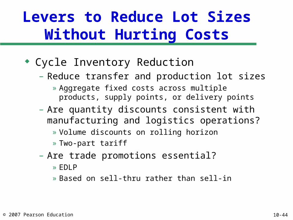
Levers to Reduce Lot Sizes Without Hurting Costs
Cycle Inventory Reduction– Reduce transfer and production lot sizes
» Aggregate fixed costs across multiple products, supply points, or delivery points
– Are quantity discounts consistent with manufacturing and logistics operations?
» Volume discounts on rolling horizon
» Two-part tariff
– Are trade promotions essential?» EDLP
» Based on sell-thru rather than sell-in
10-45© 2007 Pearson Education
Summary of Learning Objectives
How are the appropriate costs balanced to choose the optimal amount of cycle inventory in the supply chain?
What are the effects of quantity discounts on lot size and cycle inventory?
What are appropriate discounting schemes for the supply chain, taking into account cycle inventory?
What are the effects of trade promotions on lot size and cycle inventory?
What are managerial levers that can reduce lot size and cycle inventory without increasing costs?
Related Documents