SOLUTIONS 2 Choice Sets and Budget Constraints Solutions for Microeconomics: An Intuitive Approach with Calculus (International Ed.) Apart from end-of-chapter exercises provided in the student Study Guide, these solutions are provided for use by instructors. (End-of-Chapter exercises with solutions in the student Study Guide are so marked in the textbook.) The solutions may be shared by an instructor with his or her students at the instructor’s discretion. They may not be made publicly available. If posted on a course web-site, the site must be password protected and for use only by the students in the course. Reproduction and/or distribution of the solutions beyond classroom use is strictly prohibited. In most colleges, it is a violation of the student honor code for a student to share solutions to problems with peers that take the same class at a later date. • Each end-of-chapter exercise begins on a new page. This is to facilitate max- imum flexibility for instructors who may wish to share answers to some but not all exercises with their students. • If you are assigning only the A-parts of exercises in Microeconomics: An In- tuitive Approach with Calculus, you may wish to instead use the solution set created for the companion book Microeconomics: An Intuitive Approach. • Solutions to Within-Chapter Exercises are provided in the student Study Guide.

Welcome message from author
This document is posted to help you gain knowledge. Please leave a comment to let me know what you think about it! Share it to your friends and learn new things together.
Transcript

S O L U T I O N S
2Choice Sets and Budget Constraints
Solutions for Microeconomics: An IntuitiveApproach with Calculus (International Ed.)
Apart from end-of-chapter exercises provided in the student Study Guide, thesesolutions are provided for use by instructors. (End-of-Chapter exercises with
solutions in the student Study Guide are so marked in the textbook.)
The solutions may be shared by an instructor with his or her students at theinstructor’s discretion.
They may not be made publicly available.
If posted on a course web-site, the site must be password protected and foruse only by the students in the course.
Reproduction and/or distribution of the solutions beyond classroom use isstrictly prohibited.
In most colleges, it is a violation of the student honor code for a student toshare solutions to problems with peers that take the same class at a later date.
• Each end-of-chapter exercise begins on a new page. This is to facilitate max-
imum flexibility for instructors who may wish to share answers to some but
not all exercises with their students.
• If you are assigning only the A-parts of exercises in Microeconomics: An In-
tuitive Approach with Calculus, you may wish to instead use the solution set
created for the companion book Microeconomics: An Intuitive Approach.
• Solutions to Within-Chapter Exercises are provided in the student Study Guide.
Choice Sets and Budget Constraints 2
2.1 Consider a budget for good x1 (on the horizontal axis) and x2 (on the vertical axis) when your eco-
nomic circumstances are characterized by prices p1 and p2 and an exogenous income level I .
A: Draw a budget line that represents these economic circumstances and carefully label the intercepts
and slope.
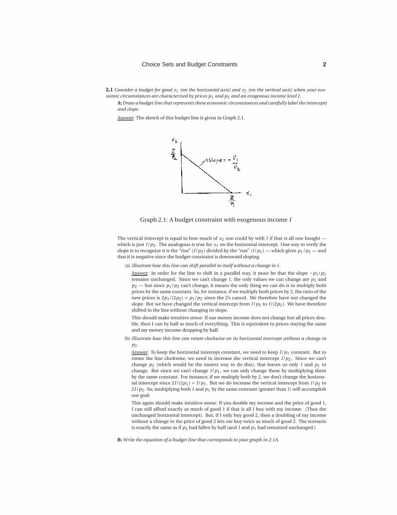
Answer: The sketch of this budget line is given in Graph 2.1.
Graph 2.1: A budget constraint with exogenous income I
The vertical intercept is equal to how much of x2 one could by with I if that is all one bought —
which is just I /p2 . The analogous is true for x1 on the horizontal intercept. One way to verify the
slope is to recognize it is the “rise” (I /p2) divided by the “run” (I /p1 ) — which gives p1/p2 — and
that it is negative since the budget constraint is downward sloping.
(a) Illustrate how this line can shift parallel to itself without a change in I .
Answer: In order for the line to shift in a parallel way, it must be that the slope −p1/p2
remains unchanged. Since we can’t change I , the only values we can change are p1 and
p2 — but since p1/p2 can’t change, it means the only thing we can do is to multiply both
prices by the same constant. So, for instance, if we multiply both prices by 2, the ratio of the
new prices is 2p1/(2p2) = p1/p2 since the 2’s cancel. We therefore have not changed the
slope. But we have changed the vertical intercept from I /p2 to I /(2p2 ). We have therefore
shifted in the line without changing its slope.
This should make intuitive sense: If our money income does not change but all prices dou-
ble, then I can by half as much of everything. This is equivalent to prices staying the same
and my money income dropping by half.
(b) Illustrate how this line can rotate clockwise on its horizontal intercept without a change in
p2 .
Answer: To keep the horizontal intercept constant, we need to keep I /p1 constant. But to
rotate the line clockwise, we need to increase the vertical intercept I /p2 . Since we can’t
change p2 (which would be the easiest way to do this), that leaves us only I and p1 to
change. But since we can’t change I /p1 , we can only change these by multiplying them
by the same constant. For instance, if we multiply both by 2, we don’t change the horizon-
tal intercept since 2I /(2p1 ) = I /p1 . But we do increase the vertical intercept from I /p2 to
2I /p2 . So, multiplying both I and p1 by the same constant (greater than 1) will accomplish
our goal.
This again should make intuitive sense: If you double my income and the price of good 1,
I can still afford exactly as much of good 1 if that is all I buy with my income. (Thus the
unchanged horizontal intercept). But, if I only buy good 2, then a doubling of my income
without a change in the price of good 2 lets me buy twice as much of good 2. The scenario
is exactly the same as if p2 had fallen by half (and I and p1 had remained unchanged.)
B: Write the equation of a budget line that corresponds to your graph in 2.1A.
3 Choice Sets and Budget Constraints
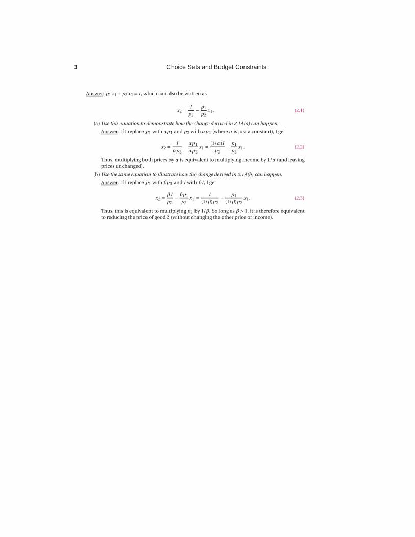
Answer: p1 x1 +p2x2 = I , which can also be written as
x2 =I
p2−
p1
p2x1. (2.1)
(a) Use this equation to demonstrate how the change derived in 2.1A(a) can happen.
Answer: If I replace p1 with αp1 and p2 with αp2 (where α is just a constant), I get
x2 =I
αp2−
αp1
αp2x1 =
(1/α)I
p2−
p1
p2x1. (2.2)
Thus, multiplying both prices by α is equivalent to multiplying income by 1/α (and leaving
prices unchanged).
(b) Use the same equation to illustrate how the change derived in 2.1A(b) can happen.
Answer: If I replace p1 with βp1 and I with βI , I get
x2 =βI
p2−
βp1
p2x1 =
I
(1/β)p2−
p1
(1/β)p2x1. (2.3)
Thus, this is equivalent to multiplying p2 by 1/β. So long as β> 1, it is therefore equivalent
to reducing the price of good 2 (without changing the other price or income).
Choice Sets and Budget Constraints 4
2.2 Suppose the only two goods in the world are peanut butter and jelly.
A: You have no exogenous income but you do own 6 jars of peanut butter and 2 jars of jelly. The price
of peanut butter is $4 per jar, and the price of jelly is $6 per jar.
(a) On a graph with jars of peanut butter on the horizontal and jars of jelly on the vertical axis,
illustrate your budget constraint.
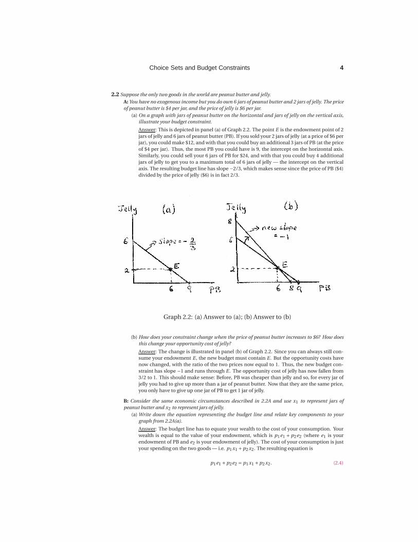
Answer: This is depicted in panel (a) of Graph 2.2. The point E is the endowment point of 2
jars of jelly and 6 jars of peanut butter (PB). If you sold your 2 jars of jelly (at a price of $6 per
jar), you could make $12, and with that you could buy an additional 3 jars of PB (at the price
of $4 per jar). Thus, the most PB you could have is 9, the intercept on the horizontal axis.
Similarly, you could sell your 6 jars of PB for $24, and with that you could buy 4 additional
jars of jelly to get you to a maximum total of 6 jars of jelly — the intercept on the vertical
axis. The resulting budget line has slope −2/3, which makes sense since the price of PB ($4)
divided by the price of jelly ($6) is in fact 2/3.
Graph 2.2: (a) Answer to (a); (b) Answer to (b)
(b) How does your constraint change when the price of peanut butter increases to $6? How does
this change your opportunity cost of jelly?
Answer: The change is illustrated in panel (b) of Graph 2.2. Since you can always still con-
sume your endowment E , the new budget must contain E . But the opportunity costs have
now changed, with the ratio of the two prices now equal to 1. Thus, the new budget con-
straint has slope −1 and runs through E . The opportunity cost of jelly has now fallen from
3/2 to 1. This should make sense: Before, PB was cheaper than jelly and so, for every jar of
jelly you had to give up more than a jar of peanut butter. Now that they are the same price,
you only have to give up one jar of PB to get 1 jar of jelly.
B: Consider the same economic circumstances described in 2.2A and use x1 to represent jars of
peanut butter and x2 to represent jars of jelly.
(a) Write down the equation representing the budget line and relate key components to your
graph from 2.2A(a).
Answer: The budget line has to equate your wealth to the cost of your consumption. Your
wealth is equal to the value of your endowment, which is p1e1 + p2e2 (where e1 is your
endowment of PB and e2 is your endowment of jelly). The cost of your consumption is just
your spending on the two goods — i.e. p1x1 +p2x2. The resulting equation is
p1e1 +p2e2 = p1x1 +p2x2. (2.4)

5 Choice Sets and Budget Constraints
When the values given in the problem are plugged in, the left hand side becomes 4(6)+6(2) =36 and the right hand side becomes 4x1 + 6x2 — resulting in the equation 36 = 4x1 + 6x2.
Taking x2 to one side, we then get
x2 = 6−2
3x1, (2.5)
which is exactly what we graphed in panel (a) of Graph 2.2 — a line with vertical intercept
of 6 and slope of −2/3.
(b) Change your equation for your budget line to reflect the change in economic circumstances
described in 2.2A(b) and show how this new equation relates to your graph in 2.2A(b).
Answer: Now the left hand side of equation (2.4) is 6(6)+6(2) = 48 while the right hand side
is 6x1 +6x2. The equation thus becomes 48 = 6x1 +6x2 or, when x2 is taken to one side,
x2 = 8−x1. (2.6)
This is an equation of a line with vertical intercept of 8 and slope of −1 — exactly what we
graphed in panel (b) of Graph 2.2.

Choice Sets and Budget Constraints 6
2.3 Any good Southern breakfast includes grits (which my wife loves) and bacon (which I love). Suppose
we allocate $60 per week to consumption of grits and bacon, that grits cost $2 per box and bacon costs $3
per package.
A: Use a graph with boxes of grits on the horizontal axis and packages of bacon on the vertical to
answer the following:
(a) Illustrate my family’s weekly budget constraint and choice set.
Answer: The graph is drawn in panel (a) of Graph 2.3.
Graph 2.3: (a) Answer to (a); (b) Answer to (c); (c) Answer to (d)
(b) Identify the opportunity cost of bacon and grits and relate these to concepts on your graph.
Answer: The opportunity cost of grits is equal to 2/3 of a package of bacon (which is equal to
the negative slope of the budget since grits appear on the horizontal axis). The opportunity
cost of a package of bacon is 3/2 of a box of grits (which is equal to the inverse of the negative
slope of the budget since bacon appears on the vertical axis).
(c) How would your graph change if a sudden appearance of a rare hog disease caused the price
of bacon to rise to $6 per package, and how does this change the opportunity cost of bacon
and grits?
Answer: This change is illustrated in panel (b) of Graph 2.3. This changes the opportunity
cost of grits to 1/3 of a package of bacon, and it changes the opportunity cost of bacon to 3
boxes of grits. This makes sense: Bacon is now 3 times as expensive as grits — so you have
to give up 3 boxes of grits for one package of bacon, or 1/3 of a package of bacon for 1 box
of grits.
(d) What happens in your graph if (instead of the change in (c)) the loss of my job caused us to
decrease our weekly budget for Southern breakfasts from $60 to $30? How does this change
the opportunity cost of bacon and grits?
Answer: The change is illustrated in panel (c) of Graph 2.3. Since relative prices have not
changed, opportunity costs have not changed. This is reflected in the fact that the slope
stays unchanged.
B: In the following, compare a mathematical approach to the graphical approach used in part A,
using x1 to represent boxes of grits and x2 to represent packages of bacon:
(a) Write down the mathematical formulation of the budget line and choice set and identify ele-
ments in the budget equation that correspond to key features of your graph from part 2.3A(a).
Answer: The budget equation is p1x1 +p2x2 = I can also be written as
x2 =I
p2−
p1
p2x1. (2.7)
With I = 60, p1 = 2 and p2 = 3, this becomes x2 = 20− (2/3)x1 — an equation with intercept
of 20 and slope of −2/3 as drawn in Graph 2.3(a).

7 Choice Sets and Budget Constraints
(b) How can you identify the opportunity cost of bacon and grits in your equation of a budget
line, and how does this relate to your answer in 2.3A(b).
Answer: The opportunity cost of x1 (grits) is simply the negative of the slope term (in terms
of units of x2). The opportunity cost of x2 (bacon) is the inverse of that.
(c) Illustrate how the budget line equation changes under the scenario of 2.3A(c) and identify the
change in opportunity costs.
Answer: Substituting the new price p2 = 6 into equation (2.7), we get x2 = 10−(1/3)x1 — an
equation with intercept of 10 and slope of −1/3 as depicted in panel (b) of Graph 2.3.
(d) Repeat (c) for the scenario in 2.3A(d).
Answer: Substituting the new income I = 30 into equation (2.7) (holding prices at p1 = 2
and p2 = 3, we get x2 = 10−(2/3)x1 — an equation with intercept of 10 and slope of −2/3 as
depicted in panel (c) of Graph 2.3.

Choice Sets and Budget Constraints 8
2.4 Suppose there are three goods in the world: x1, x2 and x3.
A: On a 3-dimensional graph, illustrate your budget constraint when your economic circumstances
are defined by p1 = 2, p2 = 6, p3 = 5 and I = 120. Carefully label intercepts.
Answer: Panel (a) of Graph 2.4 illustrates this 3-dimensional budget with each intercept given by I
divided by the price of the good on that axis.
Graph 2.4: Budgets over 3 goods: Answers to 2.4A,A(b) and A(c)
(a) What is your opportunity cost of x1 in terms of x2? What is your opportunity cost of x2 in
terms of x3?
Answer: On any slice of the graph that keeps x3 constant, the slope of the budget is−p1 /p2 =−1/3. Just as in the 2-good case, this is then the opportunity cost of x1 in terms of x2 — since
p1 is a third of p2, one gives up 1/3 of a unit of x2 when one chooses to consume 1 unit of
x1. On any vertical slice that holds x1 fixed, on the other hand, the slope is −p3/p2 =−5/6.
Thus, the opportunity cost of x3 in terms of x2 is 5/6, and the opportunity cost of x2 in terms
of x3 is the inverse — i.e. 6/5.
(b) Illustrate how your graph changes if I falls to $60. Does your answer to (a) change?
Answer: Panel (b) of Graph 2.4 illustrates this change (with the dashed plane equal to the
budget constraint graphed in panel (a).) The answer to part (a) does not change since no
prices and thus no opportunity costs changed. The new plane is parallel to the original.
(c) Illustrate how your graph changes if instead p1 rises to $4. Does your answer to part (a)
change?
Answer: Panel (c) of Graph 2.4 illustrates this change (with the dashed plane again illus-
trating the budget constraint from part (a).) Since only p1 changed, only the x1 intercept
changes. This changes the slope on any slice that holds x3 fixed from −1/3 to −2/3 — thus
doubling the opportunity cost of x1 in terms of x2. Since the slope of any slice holding x1
fixed remains unchanged, the opportunity cost of x2 in terms of x3 remains unchanged.
This makes sense since p2 and p3 did not change, leaving the tradeoff between x2 and x3
consumption unchanged.
B: Write down the equation that represents your picture in 2.4A. Then suppose that a new good x4 is
invented and priced at $1. How does your equation change? Why is it difficult to represent this new
set of economic circumstances graphically?
Answer: The equation representing the graphs is p1 x1 +p2x2 +p3 x3 = I or, plugging in the initial
prices and income relevant for panel (a), 2x1 +6x2 +5x3 = 120. With a new fourth good priced at
9 Choice Sets and Budget Constraints
1, this equation would become 2x1 +6x2 +5x3 + x4 = 120. It would be difficult to graph since we
would need to add a fourth dimension to our graphs.

Choice Sets and Budget Constraints 10
2.5 Everyday Application: Dieting and Nutrition: On a recent doctor’s visit, you have been told that you
must watch your calorie intake and must make sure you get enough vitamin E in your diet.
A: You have decided that, to make life simple, you will from now on eat only steak and carrots. A
nice steak has 250 calories and 10 units of vitamins, and a serving of carrots has 100 calories and 30
units of vitamins Your doctor’s instructions are that you must eat no more than 2000 calories and
consume at least 150 units of vitamins per day.
(a) In a graph with “servings of carrots” on the horizontal and steak on the vertical axis, illustrate
all combinations of carrots and steaks that make up a 2000 calorie a day diet.
Answer: This is illustrated as the “calorie constraint” in panel (a) of Graph 2.5. You can get
2000 calories only from steak if you eat 8 steaks and only from carrots if you eat 20 servings
of carrots. These form the intercepts of the calorie constraint.
Graph 2.5: (a) Calories and Vitamins; (b) Budget Constraint
(b) On the same graph, illustrate all the combinations of carrots and steaks that provide exactly
150 units of vitamins.
Answer: This is also illustrated in panel (a) of Graph 2.5. You can get 150 units of vitamins
from steak if you eat 15 steaks only or if you eat 5 servings of carrots only. This results in the
intercepts for the “vitamin constraint”.
(c) On this graph, shade in the bundles of carrots and steaks that satisfy both of your doctor’s
requirements.
Answer: Your doctor wants you to eat no more than 2000 calories — which means you need
to stay underneath the calorie constraint. Your doctor also wants you to get at least 150 units
of vitamin E — which means you must choose a bundle above the vitamin constraint. This
leaves you with the shaded area to choose from if you are going to satisfy both requirements.
(d) Now suppose you can buy a serving of carrots for $2 and a steak for $6. You have $26 per day
in your food budget. In your graph, illustrate your budget constraint. If you love steak and
don’t mind eating or not eating carrots, what bundle will you choose (assuming you take your
doctor’s instructions seriously)?
Answer: With $26 you can buy 13/3 steaks if that is all you buy, or you can buy 13 servings of
carrots if that is all you buy. This forms the two intercepts on your budget constraint which
has a slope of −p1/p2 =−1/3 and is depicted in panel (b) of the graph. If you really like steak
and don’t mind eating carrots one way or another, you would want to get as much steak
as possible given the constraints your doctor gave you and given your budget constraint.
This leads you to consume the bundle at the intersection of the vitamin and the budget
constraint in panel (b) — indicated by (x1,x2) in the graph. It seems from the two panels
that this bundle also satisfies the calorie constraint and lies inside the shaded region.
B: Continue with the scenario as described in part A.

11 Choice Sets and Budget Constraints
(a) Define the line you drew in A(a) mathematically.
Answer: This is given by 100x1 +250x2 = 2000 which can be written as
x2 = 8−2
5x1. (2.8)
(b) Define the line you drew in A(b) mathematically.
Answer: This is given by 30x1 +10x2 = 150 which can be written as
x2 = 15−3x1 . (2.9)
(c) In formal set notation, write down the expression that is equivalent to the shaded area in A(c).
Answer:
{(x1,x2) ∈R
2+ | 100x1 +250x2 ≤ 2000 and 30x1 +10x2 ≥ 150
}(2.10)
(d) Derive the exact bundle you indicated on your graph in A(d).
Answer: We would like to find the most amount of steak we can afford in the shaded region.
Our budget constraint is 2x1 + 6x2 = 26. Our graph suggests that this budget constraint
intersects the vitamin constraint (from equation (2.9)) within the shaded region (in which
case that intersection gives us the most steak we can afford in the shaded region). To find
this intersection, we can plug equation (2.9) into the budget constraint 2x1+6x2 = 26 to get
2x1 +6(15−3x1 ) = 26, (2.11)
and then solve for x1 to get x1 = 4. Plugging this back into either the budget constraint or
the vitamin constraint, we can get x2 = 3. We know this lies on the vitamin constraint as well
as the budget constraint. To check to make sure it lies in the shaded region, we just have to
make sure it also satisfies the doctor’s orders that you consume fewer than 2000 calories.
The bundle (x1,x2)=(4,3) results in calories of 4(100)+ 3(250) = 1150, well within doctor’s
orders.

Choice Sets and Budget Constraints 12
2.6 Everyday Application: Renting a Car versus Taking Taxis: Suppose my brother and I both go on a
week-long vacation in Cayman and, when we arrive at the airport on the island, we have to choose be-
tween either renting a car or taking a taxi to our hotel. Renting a car involves a fixed fee of $300 for the
week, with each mile driven afterwards just costing 20 cents — the price of gasoline per mile. Taking a
taxi involves no fixed fees, but each mile driven on the island during the week now costs $1 per mile.
A: Suppose both my brother and I have brought $2,000 on our trip to spend on “miles driven on the
island” and “other goods”. On a graph with miles driven on the horizontal and other consumption
on the vertical axis, illustrate my budget constraint assuming I chose to rent a car and my brother’s
budget constraint assuming he chose to take taxis.
Answer: The two budget lines are drawn in Graph 2.6. My brother could spend as much as $2,000
on other goods if he stays at the airport and does not rent any taxis, but for every mile he takes a
taxi, he gives up $1 in other good consumption. The most he can drive on the island is 2,000 miles.
As soon as I pay the $300 rental fee, I can at most consume $1,700 in other goods, but each mile
costs me only 20 cents. Thus, I can drive as much as 1700/0.2=8,500 miles.
Graph 2.6: Graphs of equations in exercise 2.6
(a) What is the opportunity cost for each mile driven that I faced?
Answer: I am renting a car — which means I give up 20 cents in other consumption per mile
driven. Thus, my opportunity cost is 20 cents. My opportunity cost does not include the
rental fee since I paid that before even getting into the car.
(b) What is the opportunity cost for each mile driven that my brother faced?
Answer: My brother is taking taxis — so he has to give up $1 in other consumption for every
mile driven. His opportunity cost is therefore $1 per mile.
B: Derive the mathematical equations for my budget constraint and my brother’s budget constraint,
and relate elements of these equations to your graphs in part A. Use x1 to denote miles driven and
x2 to denote other consumption.
Answer: My budget constraint, once I pay the rental fee, is 0.2x1 + x2 = 1700 while my brother’s
budget constraint is x1 +x2 = 2000. These can be rewritten with x2 on the left hand side as
x2 = 1700−0.2x1 for me, and (2.12)
x2 = 2000−x1 for my brother. (2.13)
The intercept terms (1700 for me and 2000 for my brother) as well as the slopes (−0.2 for me and
−1 for my brother) are as in Graph 2.6.
(a) Where in your budget equation for me can you locate the opportunity cost of a mile driven?
Answer: My opportunity cost of miles driven is simply the slope term in my budget equation
— i.e. 0.2. I give up $0.20 in other consumption for every mile driven.
13 Choice Sets and Budget Constraints
(b) Where in your budget equation for my brother can you locate the opportunity cost of a mile
driven?
Answer: My brother’s opportunity cost of miles driven is the slope term in his budget equa-
tion — i.e. 1; he gives up $1 in other consumption for every mile driven.
Choice Sets and Budget Constraints 14
2.7 Everyday Application: Watching a Bad Movie: On one of my first dates with my wife, we went to see
the movie “Spaceballs” and paid $5 per ticket.
A: Halfway through the movie, my wife said: “What on earth were you thinking? This movie sucks! I
don’t know why I let you pick movies. Let’s leave.”
(a) In trying to decide whether to stay or leave, what is the opportunity cost of staying to watch
the rest of the movie?
Answer: The opportunity cost of any activity is what we give up by undertaking that activity.
The opportunity cost of staying in the movie is whatever we would choose to do with out
time if we were not there. The price of the movie tickets that got us into the movie theater is
NOT a part of this opportunity cost — because, whether we stay or leave, we do not get that
money back.
(b) Suppose we had read a sign on the way into the theater stating “Satisfaction Guaranteed!
Don’t like the movie half way through — see the manager and get your money back!” How
does this change your answer to part (a)?
Answer: Now, in addition to giving up whatever it is we would be doing if we weren’t watch-
ing the movie, we are also giving up the price of the movie tickets. Put differently, by staying
in the movie theater, we are giving up the opportunity to get a refund — and so the cost of
the tickets is a real opportunity cost of staying.

15 Choice Sets and Budget Constraints
2.8 Everyday Application: Setting up a College Trust Fund: Suppose that you, after studying economics in
college, quickly became rich — so rich that you have nothing better to do than worry about your 16-year
old niece who can’t seem to focus on her future. Your niece currently already has a trust fund that will pay
her a nice yearly income of $50,000 starting when she is 18, and she has no other means of support.
A: You are concerned that your niece will not see the wisdom of spending a good portion of her trust
fund on a college education, and you would therefore like to use $100,000 of your wealth to change
her choice set in ways that will give her greater incentives to go to college.
(a) One option is for you to place $100,000 in a second trust fund but to restrict your niece to be
able to draw on this trust fund only for college expenses of up to $25,000 per year for four years.
On a graph with “yearly dollars spent on college education” on the horizontal axis and “yearly
dollars spent on other consumption” on the vertical, illustrate how this affects her choice set.
Answer: Panel (a) of Graph 2.7 illustrates the change in the budget constraint for this type
of trust fund. The original budget shifts out by $25,000 (denoted $25K), except that the first
$25,000 can only be used for college. Thus, the maximum amount of other consumption re-
mains $50,000 because of the stipulation that she cannot use the trust fund for non-college
expenses.
Graph 2.7: (a) Restricted Trust Fund; (b) Unrestricted; (c) Matching Trust Fund
(b) A second option is for you to simply tell your niece that you will give her $25,000 per year for
4 years and you will trust her to “do what’s right”. How does this impact her choice set?
Answer: This is depicted in panel (b) of Graph 2.7 — it is a pure income shift of $25,000 since
there are no restrictions on how the money can be used.
(c) Suppose you are wrong about your niece’s short-sightedness and she was planning on spend-
ing more than $25,000 per year from her other trust fund on college education. Do you think
she will care whether you do as described in part (a) or as described in part (b)?
Answer: If she was planning to spend more than $25K on college anyhow, then the addi-
tional bundles made possible by the trust fund in (b) are not valued by her. She would
therefore not care whether you set up the trust fund as in (a) or (b).
(d) Suppose you were right about her — she never was going to spend very much on college. Will
she care now?
Answer: Now she will care — because she would actually choose one of the bundles made
available in (b) that is not available in (a) and would therefore prefer (b) over (a).
(e) A friend of yours gives you some advice: be careful — your niece will not value her education
if she does not have to put up some of her own money for it. Sobered by this advice, you decide
to set up a different trust fund that will release 50 cents to your niece (to be spent on whatever
she wants) for every dollar that she spends on college expenses. How will this affect her choice
set?
Choice Sets and Budget Constraints 16
Answer: This is depicted in panel (c) of Graph 2.7. If your niece now spends $1 on education,
she gets 50 cents for anything she would like to spend it on — so, in effect, the opportunity
cost of getting $1 of additional education is just 50 cents. This “matching” trust fund there-
fore reduces the opportunity cost of education whereas the previous ones did not.
(f) If your niece spends $25,000 per year on college under the trust fund in part (e), can you
identify a vertical distance that represents how much you paid to achieve this outcome?
Answer: If your niece spends $25,000 on her education under the “matching” trust fund,
she will get half of that amount from your trust fund — or $12,500. This can be seen as the
vertical distance between the before and after budget constraints (in panel (c) of the graph)
at $25,000 of education spending.
B: How would you write the budget equation for each of the three alternatives discussed above?
Answer: The initial budget is x1 + x2 = 50,000. The first trust fund in (a) expands this to a budget
of
x2 = 50,000 for x1 ≤ 25,000 and x1 +x2 = 75,000 for x1 > 25,000, (2.14)
while the second trust fund in (b) expands it to x1 + x2 = 75,000. Finally, the last “matching” trust
fund in (e) (depicted in panel (c)) is 0.5x1 +x2 = 50,000.
17 Choice Sets and Budget Constraints
2.9 Business Application: Choice in Calling Plans: Phone companies used to sell minutes of phone calls
at the same price no matter how many phone calls a customer made. (We will abstract away from the fact
that they charged different prices at different times of the day and week.) More recently, phone companies,
particularly cell phone companies, have become more creative in their pricing.
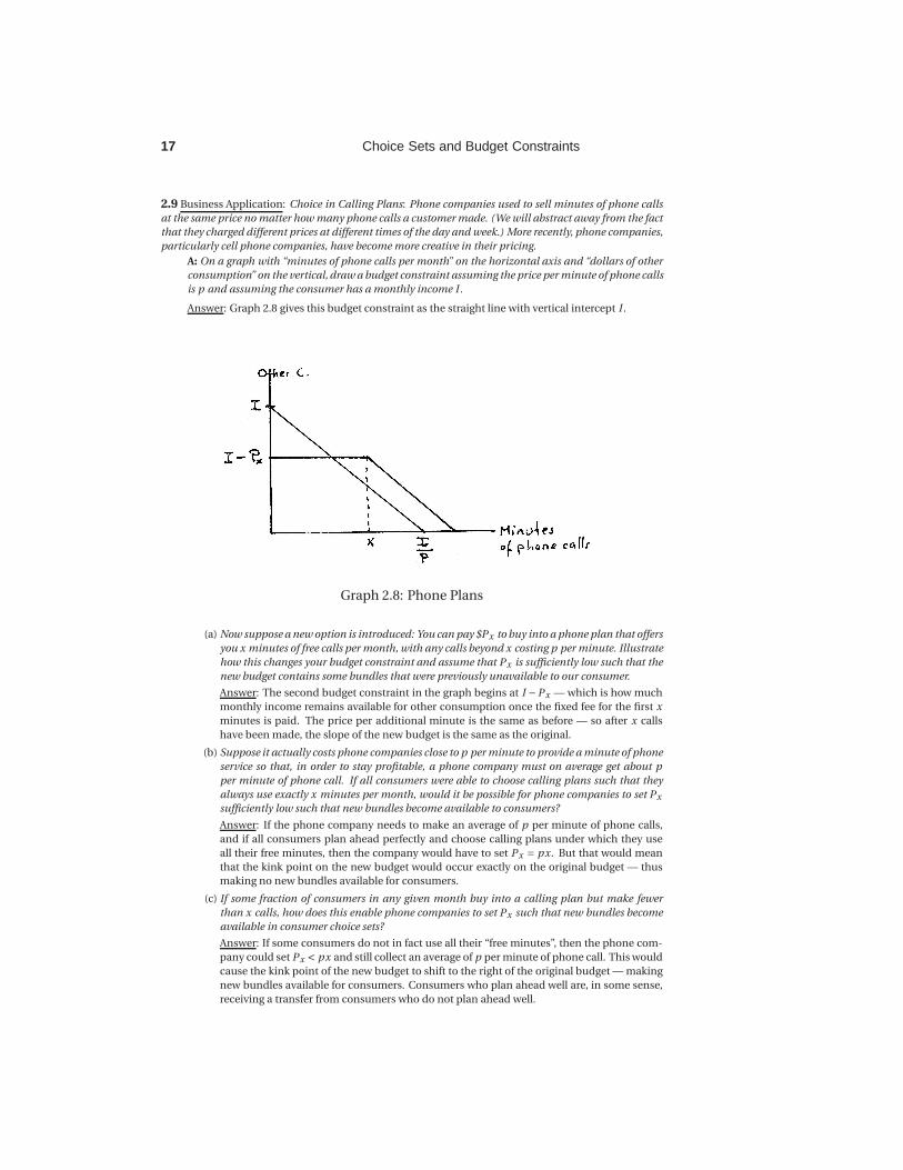
A: On a graph with “minutes of phone calls per month” on the horizontal axis and “dollars of other
consumption” on the vertical, draw a budget constraint assuming the price per minute of phone calls
is p and assuming the consumer has a monthly income I .
Answer: Graph 2.8 gives this budget constraint as the straight line with vertical intercept I .
Graph 2.8: Phone Plans
(a) Now suppose a new option is introduced: You can pay $Px to buy into a phone plan that offers
you x minutes of free calls per month, with any calls beyond x costing p per minute. Illustrate
how this changes your budget constraint and assume that Px is sufficiently low such that the
new budget contains some bundles that were previously unavailable to our consumer.
Answer: The second budget constraint in the graph begins at I −Px — which is how much
monthly income remains available for other consumption once the fixed fee for the first x
minutes is paid. The price per additional minute is the same as before — so after x calls
have been made, the slope of the new budget is the same as the original.
(b) Suppose it actually costs phone companies close to p per minute to provide a minute of phone
service so that, in order to stay profitable, a phone company must on average get about p
per minute of phone call. If all consumers were able to choose calling plans such that they
always use exactly x minutes per month, would it be possible for phone companies to set Px
sufficiently low such that new bundles become available to consumers?
Answer: If the phone company needs to make an average of p per minute of phone calls,
and if all consumers plan ahead perfectly and choose calling plans under which they use
all their free minutes, then the company would have to set Px = px. But that would mean
that the kink point on the new budget would occur exactly on the original budget — thus
making no new bundles available for consumers.
(c) If some fraction of consumers in any given month buy into a calling plan but make fewer
than x calls, how does this enable phone companies to set Px such that new bundles become
available in consumer choice sets?
Answer: If some consumers do not in fact use all their “free minutes”, then the phone com-
pany could set Px < px and still collect an average of p per minute of phone call. This would
cause the kink point of the new budget to shift to the right of the original budget — making
new bundles available for consumers. Consumers who plan ahead well are, in some sense,
receiving a transfer from consumers who do not plan ahead well.
Choice Sets and Budget Constraints 18
B: Suppose a phone company has 100,000 customers who currently buy phone minutes under the
old system that charges p per minute. Suppose it costs the company c to provide one additional
minute of phone service but the company also has fixed costs FC (that don’t vary with how many
minutes are sold) of an amount that is sufficiently high to result in zero profit. Suppose a second
identical phone company has 100,000 customers that have bought into a calling plan that charges
Px = kpx and gives customers x free minutes before charging p for minutes above x.
(a) If people on average use half their “free minutes” per month, what is k (as a functions of FC,
p,c and x) if the second company also makes zero profit?
Answer: The profit of the second company is its revenue minus its costs. Revenue is
100,000(Px ) = 100,000(kpx). (2.15)
Each customer only uses x/2 minutes, which means the cost of providing the phone min-
utes is 100,000(cx/2) = 50,000cx. The company also has to cover the fixed costs FC . So, if
profit is zero for the second company (as it is for the first), then
100000(kpx)−50000(cx)−FC = 0. (2.16)
Solving this for k, we get
k =FC
100000px+
c
2p. (2.17)
(b) If there were no fixed costs (i.e. FC = 0) but everything else was still as stated above, what does
c have to be equal to in order for the first company to make zero profit? What is k in that case?
Answer: c = p and k = 1/2. This should make intuitive sense: Under the simplified scenario,
the fact that people on average use only half their “free minutes” implies that the second
company can set its fixed fee of x minutes at half the price that the other company would
charge for consuming that many minutes.

19 Choice Sets and Budget Constraints
2.10 Business Application: Frequent Flyer Perks: Airlines offer frequent flyers different kinds of perks that
we will model here as reductions in average prices per mile flown.
A: Suppose that an airline charges 20 cents per mile flown. However, once a customer reaches 25,000
miles in a given year, the price drops to 10 cents per mile flown for each additional mile. The alter-
nate way to travel is to drive by car which costs 16 cents per mile.
(a) Consider a consumer who has a travel budget of $10,000 per year, a budget which can be spent
on the cost of getting to places as well as “other consumption” while traveling. On a graph
with “miles flown” on the horizontal axis and “other consumption” on the vertical, illustrate
the budget constraint for someone who only considers flying (and not driving) to travel desti-
nations.
Answer: Panel (a) of Graph 2.9 illustrates this budget constraint.
Graph 2.9: (a) Air travel; (b) Car travel; (c) Comparison
(b) On a similar graph with “miles driven” on the horizontal axis, illustrate the budget constraint
for someone that considers only driving (and not flying) as a means of travel.
Answer: This is illustrated in panel (b) of the graph.
(c) By overlaying these two budget constraints (changing the good on the horizontal axis simply
to “miles traveled”), can you explain how frequent flyer perks might persuade some to fly a lot
more than they otherwise would?
Answer: Panel (c) of the graph overlays the two budget constraints. If it were not for frequent
flyer miles, this consumer would never fly — because driving would be cheaper. With the
frequent flyer perks, driving is cheaper initially but becomes more expensive per additional
miles traveled if a traveler flies more than 25,000 miles. This particular consumer would
therefore either not fly at all (and just drive), or she would fly a lot because it can only make
sense to fly if she reaches the portion of the air-travel budget that crosses the car budget.
(Once we learn more about how to model tastes, we will be able to say more about whether
or not it makes sense for a traveler to fly under these circumstances.)
B: Determine where the air-travel budget from A(a) intersects the car budget from A(b).
Answer: The shallower portion of the air-travel budget (relevant for miles flown above 25,000) has
equation x2 = 7500−0.1x1 , where x2 stands for other consumption and x1 for miles traveled. The
car budget, on the other hand, has equation x2 = 10000−0.16x1 . To determine where they cross,
we can set the two equations equal to one another and solve for x1 — which gives x1 = 41,667
miles traveled. Plugging this back into either equation gives x2 = $3,333.
Choice Sets and Budget Constraints 20
2.11 Business Application: Supersizing: Suppose I run a fast-food restaurant and I know my customers
come in on a limited budget. Almost everyone that comes in for lunch buys a soft-drink. Now suppose
it costs me virtually nothing to serve a medium versus a large soft-drink, but I do incur some extra costs
when adding items (like a dessert or another side-dish) to someone’s lunch tray.
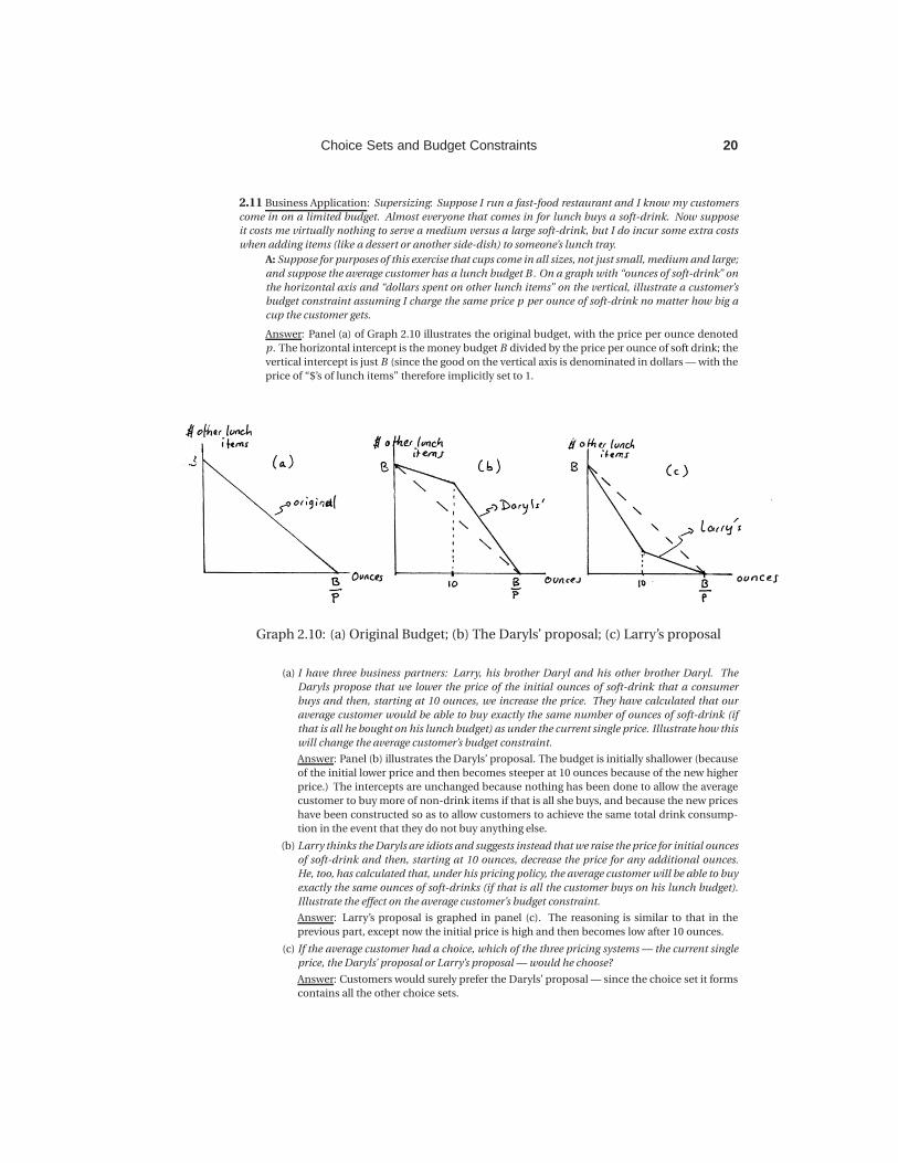
A: Suppose for purposes of this exercise that cups come in all sizes, not just small, medium and large;
and suppose the average customer has a lunch budget B . On a graph with “ounces of soft-drink” on
the horizontal axis and “dollars spent on other lunch items” on the vertical, illustrate a customer’s
budget constraint assuming I charge the same price p per ounce of soft-drink no matter how big a
cup the customer gets.
Answer: Panel (a) of Graph 2.10 illustrates the original budget, with the price per ounce denoted
p. The horizontal intercept is the money budget B divided by the price per ounce of soft drink; the
vertical intercept is just B (since the good on the vertical axis is denominated in dollars — with the
price of “$’s of lunch items” therefore implicitly set to 1.
Graph 2.10: (a) Original Budget; (b) The Daryls’ proposal; (c) Larry’s proposal
(a) I have three business partners: Larry, his brother Daryl and his other brother Daryl. The
Daryls propose that we lower the price of the initial ounces of soft-drink that a consumer
buys and then, starting at 10 ounces, we increase the price. They have calculated that our
average customer would be able to buy exactly the same number of ounces of soft-drink (if
that is all he bought on his lunch budget) as under the current single price. Illustrate how this
will change the average customer’s budget constraint.
Answer: Panel (b) illustrates the Daryls’ proposal. The budget is initially shallower (because
of the initial lower price and then becomes steeper at 10 ounces because of the new higher
price.) The intercepts are unchanged because nothing has been done to allow the average
customer to buy more of non-drink items if that is all she buys, and because the new prices
have been constructed so as to allow customers to achieve the same total drink consump-
tion in the event that they do not buy anything else.
(b) Larry thinks the Daryls are idiots and suggests instead that we raise the price for initial ounces
of soft-drink and then, starting at 10 ounces, decrease the price for any additional ounces.
He, too, has calculated that, under his pricing policy, the average customer will be able to buy
exactly the same ounces of soft-drinks (if that is all the customer buys on his lunch budget).
Illustrate the effect on the average customer’s budget constraint.
Answer: Larry’s proposal is graphed in panel (c). The reasoning is similar to that in the
previous part, except now the initial price is high and then becomes low after 10 ounces.
(c) If the average customer had a choice, which of the three pricing systems — the current single
price, the Daryls’ proposal or Larry’s proposal — would he choose?
Answer: Customers would surely prefer the Daryls’ proposal — since the choice set it forms
contains all the other choice sets.
21 Choice Sets and Budget Constraints
P.S: If you did not catch the reference to Larry, his brother Daryl and his other brother Daryl,
I recommend you rent some old versions of the 1980’s Bob Newhart Show.
B: Write down the mathematical expression for each of the three choice sets described above, letting
ounces of soft-drinks be denoted by x1 and dollars spend on other lunch items by x2.
Answer: The original budget set in panel (a) of Graph 2.10 is simply px1 + x2 = B giving a choice
set of
{(x1,x2) ∈R
2+ | x2 = B −px1
}. (2.18)
In the Daryls’ proposal, we have an initial price p′ < p for the first 10 ounces, and then a price
p′′ > p thereafter. We can calculate the x2 intercept of the steeper line following the kink point in
panel (b) of the graph by simply multiplying the x1 intercept of B /p by the slope p′′ of that line
segment to get B p′′/p. The choice set from the Daryls’ proposal could then be written as
{(x1,x2) ∈R2+ | x2 = B −p′x1 for x1 ≤ 10 and
x2 = B p ′′p −p′′x1 for x1 > 10 where p′ < p < p′′ } . (2.19)
We could even be more precise about the relationship of p′,p and p′′ . The two lines intersect at
x1 = 10, and it must therefore be the case that B −10p′ = (B p′′/p)−10p′′ . Solving this for p′, we
get that
p′ =B (p −p′′)
10p+p′′. (2.20)
Larry’s proposal begins with a price p′′ > p and then switches at 10 ounces to a price p′ < p (where
these prices have no particular relation to the prices we just used for the Daryl’s proposal). This
results in the choice set
{(x1,x2) ∈R2+ | x2 =B −p′′x1 for x1 ≤ 10 and
x2 = B p ′p −p′x1 for x1 > 10 where p′ < p < p′′ } . (2.21)
We could again derive an analogous expression for p′ in terms of p and p′′ .

Choice Sets and Budget Constraints 22
2.12 Business Application: Pricing and Quantity Discounts: Businesses often give quantity discounts.
Below, you will analyze how such discounts can impact choice sets.
A: I recently discovered that a local copy service charges our economics department $0.05 per page (or
$5 per 100 pages) for the first 10,000 copies in any given month but then reduces the price per page
to $0.035 for each additional page up to 100,000 copies and to $0.02 per each page beyond 100,000.
Suppose our department has a monthly overall budget of $5,000.
(a) Putting “pages copied in units of 100” on the horizontal axis and “dollars spent on other
goods” on the vertical, illustrate this budget constraint. Carefully label all intercepts and
slopes.
Answer: Panel (a) of Graph 2.11 traces out this budget constraint and labels the relevant
slopes and kink points.
Graph 2.11: (a) Constraint from 2.12A(a); (b) Constraint from 2.12A(b)
(b) Suppose the copy service changes its pricing policy to $0.05 per page for monthly copying up
to 20,000 and $0.025 per page for all pages if copying exceeds 20,000 per month. (Hint: Your
budget line will contain a jump.)
Answer: Panel (b) of Graph 2.11 depicts this budget. The first portion (beginning at the x2
intercept) is relatively straightforward. The second part arises for the following reason: The
problem says that, if you copy more than 2000 pages, all pages cost only $0.025 per page
— including the first 2000. Thus, when you copy 20,000 pages per month, you total bill is
$1,000. But when you copy 2001 pages, your total bill is $500.025.
(c) What is the marginal (or “additional”) cost of the first page copied after 20,000 in part (b)?
What is the marginal cost of the first page copied after 20,001 in part (b)?
Answer: The marginal cost of the first page after 20,000 is -$499.975, and the marginal cost
of the next page after that is 2.5 cents. To see the difference between these, think of the
marginal cost as the increase in the total photo-copy bill for each additional page. When
going from 20,000 to 20,001, the total bill falls by $499.975. When going from 20,001 to
20,002, the total bill rises by 2.5 cents.
B: Write down the mathematical expression for choice sets for each of the scenarios in 2.12A(a) and
2.12A(b) (using x1 to denote “pages copied in units of 100” and x2 to denote “dollars spent on other
goods”).
Answer: The choice set in (a) is
23 Choice Sets and Budget Constraints
{(x1,x2) ∈R2+ | x2 = 5000−5x1 for x1 ≤ 100 and
x2 = 4850−3.5x1 for 100 < x1 ≤ 1000 and
x2 = 3350−2x1 for x1 > 1000 }. (2.22)
The choice set in (b) is
{(x1,x2) ∈R2+ | x2 = 5000−5x1 for x1 ≤ 200 and
x2 = 5000−2.5x1 for x1 > 200 } . (2.23)
Choice Sets and Budget Constraints 24
2.13 Policy Application: Tax Deductions and Tax Credits: In the U.S. income tax code, a number of ex-
penditures are “deductible”. For most tax payers, the largest tax deduction comes from the portion of the
income tax code that permits taxpayers to deduct home mortgage interest (on both a primary and a va-
cation home). This means that taxpayers who use this deduction do not have to pay income tax on the
portion of their income that is spent on paying interest on their home mortgage(s). For purposes of this
exercise, assume that the entire yearly price of housing is interest expense.
A: True or False: For someone whose marginal tax rate is 33%, this means that the government is
subsidizing roughly one third of his interest/house payments.
Answer: Consider someone who pays $10,000 per year in mortgage interest. When this person
deducts $10,000, it means that he does not have to pay the 33% income tax on that amount. In
other words, by deducting $10,000 in mortgage interest, the person reduces his tax obligation by
$3,333.33. Thus, the government is returning 33 cents for every dollar in interest payments made —
effectively causing the opportunity cost of paying $1 in home mortgage interest to be equal to 66.67
cents. So the statement is true.
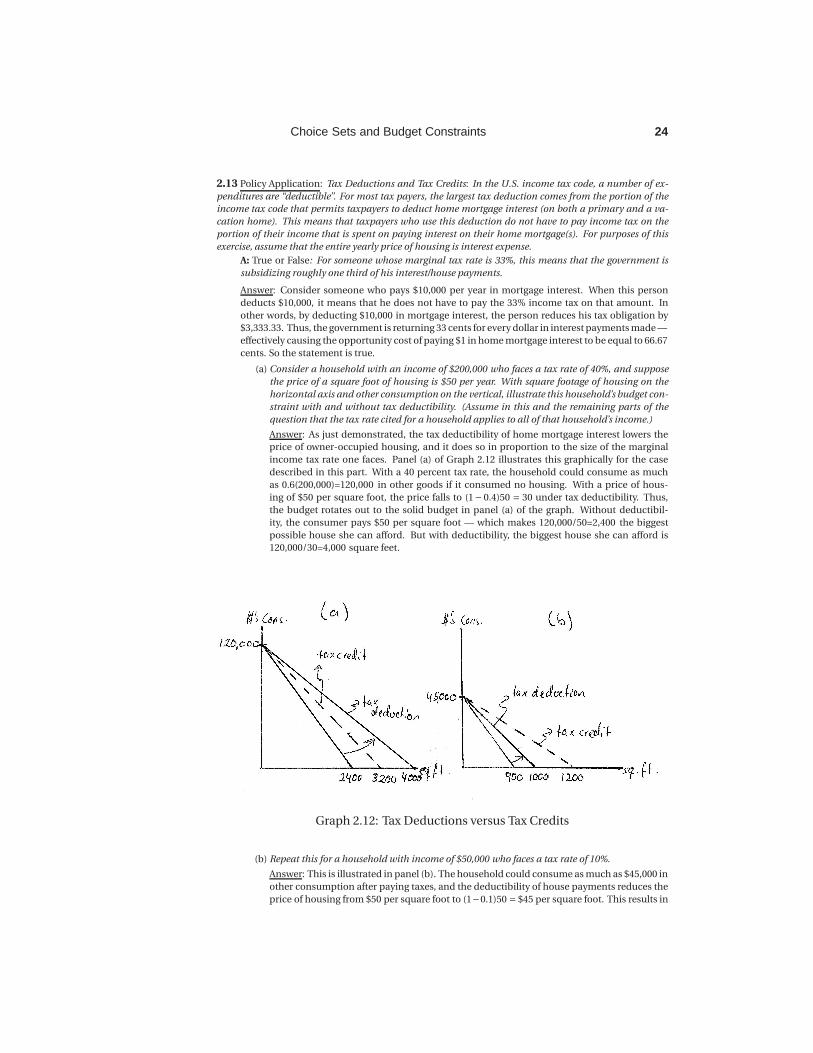
(a) Consider a household with an income of $200,000 who faces a tax rate of 40%, and suppose
the price of a square foot of housing is $50 per year. With square footage of housing on the
horizontal axis and other consumption on the vertical, illustrate this household’s budget con-
straint with and without tax deductibility. (Assume in this and the remaining parts of the
question that the tax rate cited for a household applies to all of that household’s income.)
Answer: As just demonstrated, the tax deductibility of home mortgage interest lowers the
price of owner-occupied housing, and it does so in proportion to the size of the marginal
income tax rate one faces. Panel (a) of Graph 2.12 illustrates this graphically for the case
described in this part. With a 40 percent tax rate, the household could consume as much
as 0.6(200,000)=120,000 in other goods if it consumed no housing. With a price of hous-
ing of $50 per square foot, the price falls to (1− 0.4)50 = 30 under tax deductibility. Thus,
the budget rotates out to the solid budget in panel (a) of the graph. Without deductibil-
ity, the consumer pays $50 per square foot — which makes 120,000/50=2,400 the biggest
possible house she can afford. But with deductibility, the biggest house she can afford is
120,000/30=4,000 square feet.
Graph 2.12: Tax Deductions versus Tax Credits
(b) Repeat this for a household with income of $50,000 who faces a tax rate of 10%.
Answer: This is illustrated in panel (b). The household could consume as much as $45,000 in
other consumption after paying taxes, and the deductibility of house payments reduces the
price of housing from $50 per square foot to (1−0.1)50 = $45 per square foot. This results in
25 Choice Sets and Budget Constraints
the indicated rotation of the budget from the lower to the higher solid line in the graph. The
rotation is smaller in magnitude because the impact of deductibility on the after-tax price
of housing is smaller. Without deductibility, the biggest affordable house is 45,000/50=900
square feet, while with deductibility the biggest possible house is 45,000/45=1,000 square
feet.
(c) An alternative way for the government to encourage home ownership would be to offer a tax
credit instead of a tax deduction. A tax credit would allow all taxpayers to subtract a fraction
k of their annual mortgage payments directly from the tax bill they would otherwise owe.
(Note: Be careful — a tax credit is deducted from tax payments that are due, not from the
taxable income.) For the households in (a) and (b), illustrate how this alters their budget if
k = 0.25.
Answer: This is illustrated in the two panels of Graph 2.12 — in panel (a) for the higher in-
come household, and in panel (b) for the lower income household. By subsidizing housing
through a credit rather than a deduction, the government has reduced the price of hous-
ing by the same amount (k) for everyone. In the case of deductibility, the government had
made the price subsidy dependent on one’s tax rate — with those facing higher tax rates also
getting a higher subsidy. The price of housing how falls from $50 to (1−0.25)50 = $37.50 —
which makes the largest affordable house for the wealthier household 120,000/37.5=3,200
square feet and, for the poorer household, 45,000/37.5=1,200 square feet. Thus, the poorer
household benefits more from the credit when k = 0.25 while the richer household benefits
more from the deduction.
(d) Assuming that a tax deductibility program costs the same in lost tax revenues as a tax credit
program, who would favor which program?
Answer: People facing higher marginal tax rates would favor the deductibility program while
people facing lower marginal tax rates would favor the tax credit.
B: Let x1 and x2 represent square feet of housing and other consumption, and let the price of a square
foot of housing be denoted p.
(a) Suppose a household faces a tax rate t for all income, and suppose the entire annual house
payment a household makes is deductible. What is the household’s budget constraint?
Answer: The budget constraint would be x2 = (1− t )I − (1− t )px1 .
(b) Now write down the budget constraint under a tax credit as described above.
Answer: The budget constraint would now be x2 = (1− t )I − (1−k)px1 .

Choice Sets and Budget Constraints 26
2.14 Policy Application: Public Schools and Private School Vouchers: Consider a simple model of how
economic circumstances are changed when the government enters the education market.
A: Suppose a household has an after-tax income of $50,000 and consider its budget constraint with
“dollars of education services” on the horizontal axis and “dollars of other consumption” on the ver-
tical. Begin by drawing the household’s budget line (given that you can infer a price for each of the
goods on the axes from the way these goods are defined) assuming that the household can buy any
level of school spending on the private market.
Answer: The budget line in this case is straightforward and illustrated in panel (a) of Graph 2.13 as
the constraint labeled “private school constraint”.
Graph 2.13: (a) Tax on Grits; (b) Lump Sum Rebate
(a) Now suppose the government uses its existing tax revenues to fund a public school at $7,500
per pupil; i.e. it funds a school that anyone can attend for free and that provides $7,500 in
education services. Illustrate how this changes the choice set.(Hint: One additional point will
appear in the choice set.)
Answer: Since public education is free (and paid for from existing tax revenues — i.e. no
new taxes are imposed), it now becomes possible to consume a public school that offers
$7,500 of educational services while still consuming $50,000 in other consumption. This
adds an additional bundle to the choice set — the bundle (7,500, 50,000) denoted “public
school bundle” in panel (a) of the graph.
(b) Continue to assume that private school services of any quantity could be purchased but only
if the child does not attend public schools. Can you think of how the availability of free pub-
lic schools might cause some children to receive more educational services than before they
would in the absence of public schools? Can you think of how some children might receive
fewer educational services once public schools are introduced?
Answer: If a household purchased less than $7,500 in education services for a child prior to
the introduction of the public school, it seems likely that the household would jump at the
opportunity to increase both consumption of other goods and consumption of education
services by switching to the public education bundle. At the same time, if a household pur-
chased more than $7,500 in education services prior to the introduction of public schools,
it is plausible that this household will also switch to the public school bundle — because,
while it would mean less eduction service for the child, it would also mean a large increase
in other consumption. (We will be able to be more precise once we introduce a model of
tastes.)
(c) Now suppose the government allows an option: either a parent can send her child to the pub-
lic school or she can take a voucher to a private school and use it for partial payment of private
school tuition. Assume that the voucher is worth $7,500 per year; i.e. it can be used to pay for

27 Choice Sets and Budget Constraints
up to $7,500 in private school tuition. How does this change the budget constraint? Do you
still think it is possible that some children will receive less education than they would if the
government did not get involved at all (i.e. no public schools and no vouchers)?
Answer: The voucher becomes equivalent to cash so long as at least $7,500 is spent on
education services. This results in the budget constraint depicted in panel (b) of Graph
2.13. Since one cannot use the voucher to increase other consumption beyond $50,000, the
voucher does not make any private consumption above $50,000 possible. However, it does
make it possible to consume any level of education service between 0 and $7,500 without
incurring any opportunity cost in terms of other consumption. Only once the full voucher
is used and $7,500 in education services have been bought will the household be giving up
a dollar in other consumption for every additional dollar in education services.
It is easy to see how this will lead some parents to choose more education for their chil-
dren (just as it was true that the introduction of the public school bundle gets some parents
to increase the education services consumed by their children.) But the reverse no longer
appears likely — if someone choses more than $7,500 in education services in the absence
of public schools and vouchers, the effective increase in household income implied by the
voucher/public school combination makes it unlikely that such a household will reduce the
education services given to her child. (Again, we will be able to be more precise once we
introduce tastes — and we will see that it would take unrealistic tastes for this to happen.)
B: Letting dollars of education services be denoted by x1 and dollars of other consumption by x2,
formally define the choice set with just the public school (and a private school market) as well as the
choice set with private school vouchers defined above.
Answer: The first choice set (in panel (a) of the graph) is formally defined as
{(x1,x2) ∈R
2+ | x2 ≤ 50000−x1 or (x1,x2) = (7500,50000)
}, (2.24)
while the introduction of vouchers changes the choice set to
{(x1,x2) ∈R2+ | x2 = 50000 for x1 ≤ 7500 and
x2 = 57500−x1 for x1 > 7500 }. (2.25)
Choice Sets and Budget Constraints 28
2.15 Policy Application: Taxing Goods versus Lump Sum Taxes: I have finally convinced my local con-
gressman that my wife’s taste for grits are nuts and that the world should be protected from too much grits
consumption. As a result, my congressman has agreed to sponsor new legislation to tax grits consumption
which will raise the price of grits from $2 per box to $4 per box. We carefully observe my wife’s shopping
behavior and notice with pleasure that she now purchases 10 boxes of grits per month rather than her
previous 15 boxes.
A: Putting “boxes of grits per month” on the horizontal and “dollars of other consumption” on the
vertical, illustrate my wife’s budget line before and after the tax is imposed. (You can simply denote
income by I .)
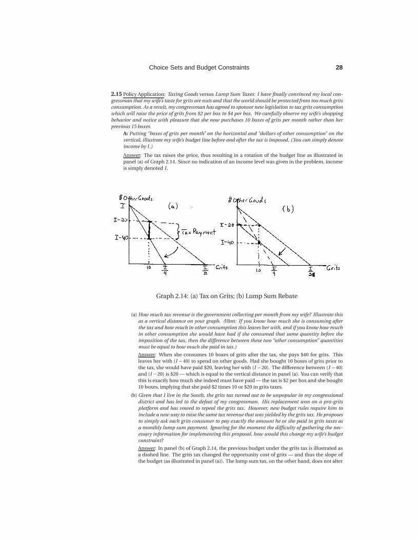
Answer: The tax raises the price, thus resulting in a rotation of the budget line as illustrated in
panel (a) of Graph 2.14. Since no indication of an income level was given in the problem, income
is simply denoted I .
Graph 2.14: (a) Tax on Grits; (b) Lump Sum Rebate
(a) How much tax revenue is the government collecting per month from my wife? Illustrate this
as a vertical distance on your graph. (Hint: If you know how much she is consuming after
the tax and how much in other consumption this leaves her with, and if you know how much
in other consumption she would have had if she consumed that same quantity before the
imposition of the tax, then the difference between these two “other consumption” quantities
must be equal to how much she paid in tax.)
Answer: When she consumes 10 boxes of grits after the tax, she pays $40 for grits. This
leaves her with (I −40) to spend on other goods. Had she bought 10 boxes of grits prior to
the tax, she would have paid $20, leaving her with (I −20). The difference between (I −40)
and (I −20) is $20 — which is equal to the vertical distance in panel (a). You can verify that
this is exactly how much she indeed must have paid — the tax is $2 per box and she bought
10 boxes, implying that she paid $2 times 10 or $20 in grits taxes.
(b) Given that I live in the South, the grits tax turned out to be unpopular in my congressional
district and has led to the defeat of my congressman. His replacement won on a pro-grits
platform and has vowed to repeal the grits tax. However, new budget rules require him to
include a new way to raise the same tax revenue that was yielded by the grits tax. He proposes
to simply ask each grits consumer to pay exactly the amount he or she paid in grits taxes as
a monthly lump sum payment. Ignoring for the moment the difficulty of gathering the nec-
essary information for implementing this proposal, how would this change my wife’s budget
constraint?
Answer: In panel (b) of Graph 2.14, the previous budget under the grits tax is illustrated as
a dashed line. The grits tax changed the opportunity cost of grits — and thus the slope of
the budget (as illustrated in panel (a)). The lump sum tax, on the other hand, does not alter

29 Choice Sets and Budget Constraints
opportunity costs but simply reduces income by $20, the amount of grits taxes my wife paid
under the grits tax. This change is illustrated in panel (b).
B: State the equations for the budget constraints you derived in A(a) and A(b), letting grits be denoted
by x1 and other consumption by x2.
Answer: The initial (before-tax) budget was x2 = I − 2x1 which becomes x2 = I − 4x1 after the
imposition of the grits tax. The lump sum tax budget constraint, on the other hand, is x2 = I −20−2x1.
Choice Sets and Budget Constraints 30
2.16 Policy Application: Public Housing and Housing Subsidies: For a long period, the U.S. government
focused its attempts to meet housing needs among the poor through public housing programs. Eligible
families could get on waiting lists to apply for an apartment in a public housing development and would
be offered a particular apartment as they moved to the top of the waiting list.
A: Suppose a particular family has a monthly income of $1,500 and is offered a 1,500 square foot
public housing apartment for $375 in monthly rent. Alternatively, the family could choose to rent
housing in the private market for $0.50 per square foot.
(a) Illustrate all the bundles in this family’s choice set of “square feet of housing” (on the horizon-
tal axis) and “dollars of monthly other goods consumption” (on the vertical axis).
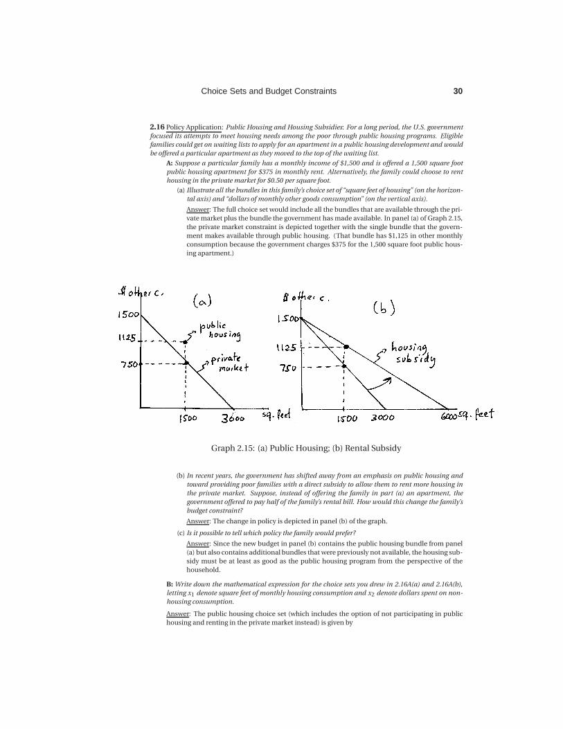
Answer: The full choice set would include all the bundles that are available through the pri-
vate market plus the bundle the government has made available. In panel (a) of Graph 2.15,
the private market constraint is depicted together with the single bundle that the govern-
ment makes available through public housing. (That bundle has $1,125 in other monthly
consumption because the government charges $375 for the 1,500 square foot public hous-
ing apartment.)
Graph 2.15: (a) Public Housing; (b) Rental Subsidy
(b) In recent years, the government has shifted away from an emphasis on public housing and
toward providing poor families with a direct subsidy to allow them to rent more housing in
the private market. Suppose, instead of offering the family in part (a) an apartment, the
government offered to pay half of the family’s rental bill. How would this change the family’s
budget constraint?
Answer: The change in policy is depicted in panel (b) of the graph.
(c) Is it possible to tell which policy the family would prefer?
Answer: Since the new budget in panel (b) contains the public housing bundle from panel
(a) but also contains additional bundles that were previously not available, the housing sub-
sidy must be at least as good as the public housing program from the perspective of the
household.
B: Write down the mathematical expression for the choice sets you drew in 2.16A(a) and 2.16A(b),
letting x1 denote square feet of monthly housing consumption and x2 denote dollars spent on non-
housing consumption.
Answer: The public housing choice set (which includes the option of not participating in public
housing and renting in the private market instead) is given by

31 Choice Sets and Budget Constraints
{(x1,x2) ∈R
2+ | (x1,x2)= (1500,1125) or x2 ≤ 1500−0.5x1
}. (2.26)
The rental subsidy in panel (b), on the other hand, creates the choice set
{(x1,x2) ∈R
2+ | x2 ≤ 1500−0.25x1
}. (2.27)

Choice Sets and Budget Constraints 32
2.17 Policy Application: Food Stamp Programs and other Types of Subsidies: The U.S. government has a
food stamp program for families whose income falls below a certain poverty threshold. Food stamps have
a dollar value that can be used at supermarkets for food purchases as if the stamps were cash, but the food
stamps cannot be used for anything other than food.
A: Suppose the program provides $500 of food stamps per month to a particular family that has a
fixed income of $1,000 per month.
(a) With “dollars spent on food” on the horizontal axis and “dollars spent on non-food items” on
the vertical, illustrate this family’s monthly budget constraint. How does the opportunity cost
of food change along the budget constraint you have drawn?
Answer: Panel (a) of Graph 2.16 illustrates the original budget — with intercept 1,000 on
each axis. It then illustrates the new budget under the food stamp program. Since food
stamps can only be spent on food, the “other goods” intercept does not change — owning
some food stamps still only allows households to spend what they previously had on other
goods. However, the family is now able to buy $1,000 in other goods even as it buys food —
because it can use the food stamps on the first $500 worth of food and still have all its other
income left for other consumption. Only after all the food stamps are spent — i.e. after the
family has bought $500 worth of food — does the family give up other consumption when
consuming additional food. As a result, the opportunity cost of food is zero until the food
stamps are gone, and it is 1 after that. That is, after the food stamps are gone, the family
gives up $1 in other consumption for every $1 of food it purchases.
Graph 2.16: (a) Food Stamps; (b) Cash; (c) Re-imburse half
(b) How would this family’s budget constraint differ if the government replaced the food stamp
program with a cash subsidy program that simply gave this family $500 in cash instead of
$500 in food stamps? Which would the family prefer, and what does your answer depend on?
Answer: In this case, the original budget would simply shift out by $500 as depicted in panel
(b). If the family consumes more than $500 of food under the food stamp program, it would
not seem like anything really changes under the cash subsidy. (We can show this more for-
mally once we introduce a model of tastes). If, on the other hand, the family consumes $500
of food under the food stamps, it may well be that it would prefer to get cash instead so that
it can consume more other goods instead.
(c) How would the budget constraint change if the government simply agreed to reimburse the
family for half its food expenses?
Answer: In this case, the government essentially reduces the price of $1 of food to 50 cents
because whenever $1 is spent on food, the government reimburses the family 50 cents. The
resulting change in the family budget is then depicted in panel (c) of the graph.
(d) If the government spends the same amount for this family on the program described in (c)
as it did on the food stamp program, how much food will the family consume? Illustrate the
33 Choice Sets and Budget Constraints
amount the government is spending as a vertical distance between the budget lines you have
drawn.
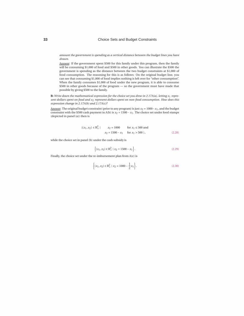
Answer: If the government spent $500 for this family under this program, then the family
will be consuming $1,000 of food and $500 in other goods. You can illustrate the $500 the
government is spending as the distance between the two budget constraints at $1,000 of
food consumption. The reasoning for this is as follows: On the original budget line, you
can see that consuming $1,000 of food implies nothing is left over for “other consumption”.
When the family consumes $1,000 of food under the new program, it is able to consume
$500 in other goods because of the program — so the government must have made that
possible by giving $500 to the family.
B: Write down the mathematical expression for the choice set you drew in 2.17A(a), letting x1 repre-
sent dollars spent on food and x2 represent dollars spent on non-food consumption. How does this
expression change in 2.17A(b) and 2.17A(c)?
Answer: The original budget constraint (prior to any program) is just x2 = 1000−x1 , and the budget
constraint with the $500 cash payment in A(b) is x2 = 1500−x1 . The choice set under food stamps
(depicted in panel (a)) then is
{(x1,x2) ∈R2+ | x2 = 1000 for x1 ≤ 500 and
x2 = 1500−x1 for x1 > 500 }, (2.28)
while the choice set in panel (b) under the cash subsidy is
{(x1,x2) ∈R
2+ | x2 = 1500−x1
}. (2.29)
Finally, the choice set under the re-imbursement plan from A(c) is
{(x1,x2) ∈R
2+ | x2 = 1000−
1
2x1
}. (2.30)
Related Documents