Choice of θ and mean-square exponential stability in the stochastic theta method of stochastic differential equations

This article appeared in a journal published by Elsevier. The attachedcopy is furnished to the author for internal non-commercial researchand education use, including for instruction at the authors institution

and sharing with colleagues.

Other uses, including reproduction and distribution, or selling orlicensing copies, or posting to personal, institutional or third party

websites are prohibited.

In most cases authors are permitted to post their version of thearticle (e.g. in Word or Tex form) to their personal website orinstitutional repository. Authors requiring further information

regarding Elsevier’s archiving and manuscript policies areencouraged to visit:

http://www.elsevier.com/authorsrights

Author's personal copy

Journal of Computational and Applied Mathematics 255 (2014) 837–847

Contents lists available at ScienceDirect

Journal of Computational and AppliedMathematics

journal homepage: www.elsevier.com/locate/cam

Choice of θ and mean-square exponential stability in thestochastic theta method of stochastic differential equations

Xiaofeng Zong, Fuke Wu ∗

School of Mathematics and Statistics, Huazhong University of Science and Technology, Wuhan, 430074, PR China

a r t i c l e i n f o

Article history:Received 30 August 2012Received in revised form 12 January 2013

Keywords:SDEsSTMEMBEMMean-square exponential stability

a b s t r a c t

This paper examines the relationship of choice of θ and mean-square exponential stabilityin the stochastic thetamethod (STM) of stochastic differential equations (SDEs) andmainlyincludes the following three results: (i) under the linear growth condition for the drift term,when θ ∈ [0, 1/2), the STM may preserve the mean-square exponential stability of theexact solution, but the counterexample shows that the STM cannot reproduce this stabilitywithout this linear growth condition; (ii) when θ ∈ (1/2, 1), without the linear growthcondition for the drift term, the STMmay reproduce themean-square exponential stabilityof the exact solution, but the bound of the Lyapunov exponent cannot be preserved;(iii) when θ = 1 (this STM is called as the backward Euler–Maruyama (BEM) method),the STM can reproduce not only the mean-square exponential stability, but also the boundof the Lyapunov exponent. This paper also gives the sufficient and necessary conditions ofthemean-square exponential stability of the STM for the linear SDEwhen θ ∈ [0, 1/2) andθ ∈ [1/2, 1], respectively, and the simulations also illustrate these theoretical results.

© 2013 Elsevier B.V. All rights reserved.

1. Introduction and motivation

SDEs have been studied for more than fifty years due to the role, played in describing signal processing, queueing net-works, production planning, biological systems, ecosystems, financial engineering and control. Since most SDEs cannot besolved explicitly, numerical methods have become the efficient method to examine the properties of these stochastic sys-tems. Stability theory of numerical solutions is one of the central problems in numerical analysis [1,2]. Stability analysis ofnumericalmethods for SDEs, includingmoment stability, almost sure stability, stability in distribution, has recently receiveda great deal of attention (for example, see [3–9] and the related references therein).

The main aim of this paper is to study the mean-square exponential stability of STM for the n-dimensional SDEdx(t) = f (x(t))dt + g(x(t))dW (t), t ≥ 0, (1)

with the initial value 0 = x(0) = x0 ∈ Rn, where W (t) is a scalar Brownian motion and functions f , g : Rn→ Rn are

smooth enough for the SDE (1) to have a unique global solution x(t) on [0, ∞) (see, for example, [10] for details). Assumethat f (0) = g(0) = 0 for the purpose of stability. Applying the STM to (1) gives (see [11,12,7,13])

xk+1 = xk + (1 − θ)∆f (xk) + θ∆f (xk+1) + g(xk)∆Wk k = 1, 2, . . . , (2)where ∆ > 0 is the constant stepsize, θ ∈ [0, 1] is a fixed parameter, and ∆Wk := W ((k + 1)∆) − W (k∆) is the Brownianincrement. It is well-known that the STM includes the EMmethod (θ = 0), the trapezoidal method (θ = 1/2) and the BEMmethod (θ = 1).

This work was supported in part by the National Natural Science Foundations of China (Grant Nos. 11001091 and 61134012) and in part by Programfor New Century Excellent Talents in University.∗ Corresponding author. Tel.: +86 27 87557195; fax: +86 27 87543231.

E-mail addresses: [email protected] (X. Zong), [email protected], [email protected] (F. Wu).

0377-0427/$ – see front matter© 2013 Elsevier B.V. All rights reserved.http://dx.doi.org/10.1016/j.cam.2013.07.007

Author's personal copy

838 X. Zong, F. Wu / Journal of Computational and Applied Mathematics 255 (2014) 837–847

Higham [12] studied the mean-square and almost sure stability of the STM of linear scalar SDEs and obtained that whenθ ∈ [1/2, 1], the STM is stochastically A-stable, i.e., it preserves the mean-square stability of the test linear SDEs. Thisproperty is similar to the deterministic cases. The stability of numerical methods for linear stochastic matrix equations hasbeen studied by [11,14,15]. For nonlinear SDEs, Highamet al. [13] showed that the BEMand the split-step BEMcan reproducethe mean-square exponential stability of SDEs with global Lipschitz condition for sufficiently small stepsize. For sufficientlysmall p, [7] examined the pth moment stability of the STM for the linear and nonlinear SDEs and showed that if the driftcoefficient satisfies the one-sided Lipschitz condition, the BEMmethod can reproduce the almost sure exponential stabilityof the exact solution. Huang [16] investigated the split-step STM for SDEs and proved that the split-step STM with θ > 1/2may preserve the mean-square exponential stability of the exact solutions under a coupled condition on the drift anddiffusion coefficients. Recently, Szpruch et al. [17] and Chen and Wu [18] examined the stability of STM for SDEs under thelocal Lipschitz conditions. Szpruch et al. examined the almost sure asymptotic stability of STM under monotone conditions.For sufficiently small stepsize, by using discrete semimartingale convergence theorem, Chen and Wu [18] investigated thealmost sure exponential stability of the STM and proved that when θ ∈ (1/2, 1], the STM may preserve the stability of theexact solutions without the linear growth condition for the drift coefficient.

This paper will examine the mean-square exponential stability of the STM for SDEs and obtain the following results:(i) under the linear growth condition for the drift term, when θ ∈ [0, 1/2), the STM may preserve the mean-square

exponential stability of the exact solution, but the counterexample shows that the STM cannot reproduce this stabilitywithout this linear growth condition;

(ii) when θ ∈ (1/2, 1), without the linear growth condition for the drift term, the STM may reproduce the mean-squareexponential stability of the exact solution, but the bound of the Lyapunov exponent cannot be preserved;

(iii) when θ = 1 (the BEM), the STM can reproduce not only the mean-square exponential stability, but also the bound ofthe Lyapunov exponent.

This paper also presents the sufficient and necessary conditions of the mean-square exponential stability of the STM for thelinear SDE when θ ∈ [0, 1/2] and θ ∈ (1/2, 1], respectively, and gives the simulations.

The rest of the paper is arranged as follows. The next section introduces some notations and definitions. Section 3examines the stability of the STM for θ ∈ [0, 1/2) and presents a counterexample to show that this STM cannot reproducethe mean-square stability of the exact solution without the linear growth condition. Section 4 discusses mean-squareexponential stability of the STM for θ ∈ (1/2, 1]. Section 5 presents the sufficient and necessary conditions of the mean-square exponential stability of the STM for the linear SDE and gives the simulations.

2. Notations and definitions

Throughout this paper, let (Ω, F, P) be a complete probability space with a filtration Ftt≥0 satisfying the usualconditions, that is, it is right continuous and increasing while F0 contains all P-null sets. Let W (t) be a scalar Brownianmotion defined on this probability space. Let | · | denote both the Euclidean norms in Rn. The inner product of x, y in Rn isdenoted by ⟨x, y⟩. a ∨ b represents maxa, b and a ∧ b denotes mina, b.

When the asymptotic stability of SDEs is studied, without loss of generality, it is convenient to assume that the initialcondition is deterministic. It can be extended to a random variable (see, for example, [10]). Let us now give the definitionson the mean-square exponential stability for the SDE (1) and its STM numerical solution.

Definition 2.1. Eq. (1) is said to be mean-square exponentially stable if there exists a constant η > 0 such that

lim supt→∞

1tlog(E|x(t)|2) ≤ −η

for any bounded initial value x(0) ∈ Rn.

Definition 2.2. The approximate solution xk defined by (2) is said to be mean-square exponentially stable if there exists aconstant η > 0 such that

lim supk→∞

log(E|xk|2)k∆

≤ −η

for any bounded x0 ∈ Rn.

As a standing hypothesis, we impose the local Lipschitz condition on the coefficients f and g .

Assumption 2.1. f , g satisfy the local Lipschitz condition, that is, for each j > 0, there exists a positive constant Cj such that

|f (x) − f (y)| ∨ |g(x) − g(y)| ≤ Cj|x − y|,

for all x, y ∈ Rn with |x| ∨ |y| ≤ j.

To examine the mean-square exponential stability of the STM (2), let us present the following mean-square exponentialstability of the exact solutions of Eq. (1) (see Mao [19,10]).

Author's personal copy

X. Zong, F. Wu / Journal of Computational and Applied Mathematics 255 (2014) 837–847 839

Theorem 2.1. Let Assumption 2.1 hold. Assume there exist two constants µ, σ such that for any x ∈ Rn,

xT f (x) ≤ µ|x|2, (3)|g(x)| ≤ σ |x|. (4)

If

2µ + σ 2 < 0, (5)

then Eq. (1) obeys

lim supt→∞

1tlogE|x(t)|2 ≤ 2µ + σ 2,

namely, Eq. (1) is mean-square exponentially stable.

3. Mean-square stability of the STM (2) for θ ∈ [0, 1/2)

Since the STM is semi-implicit when θ = 0, to ensure that this method is well defined, let us impose the one-sidedLipschitz condition on f (see, for example, [1]): there exists a constant b such that for any x, y ∈ Rn,

⟨x − y, f (x) − f (y)⟩ ≤ b|x − y|2. (6)

This, together with θb∆ < 1, ensures that (2) is well defined, that is, the STM (2) can be solved uniquely for xk+1. We alsoimpose the linear growth condition for f

|f (x)| ≤ K |x|, ∀ x ∈ Rn. (7)

Theorem 3.1. Let conditions (3)–(7) and Assumption 2.1 hold. For θ ∈ [0, 1/2), there exists a ∆∗ > 0 such that if ∆ < ∆∗, theSTM (2) obeys

lim supk→∞

1k∆

logE|xk|2 ≤ −γ∆, (8)

where γ∆ is a positive constant with the property

lim∆→0

γ∆ = −(2µ + σ 2) > 0, (9)

namely, the STM (2) is mean-square exponentially stable.

Proof. Applying conditions (3), (4) and (7) to (2) gives

|xk+1|2

= ⟨xk+1, f (xk+1)⟩θ∆ + ⟨xk+1, xk + (1 − θ)∆f (xk) + g(xk)∆Wk⟩

≤

12

+ µ∆θ

|xk+1|

2+

12[1 + 2(1 − θ)∆µ + (1 − θ)2∆2K 2

+ σ 2∆]|xk|2 +12mk, (10)

where mk = g(xk)2(∆Wk2− ∆) + 2⟨xk + (1 − θ)∆f (xk), g(xk)∆Wk⟩. It follows that

(1 − 2µ∆θ)|xk+1|2

≤ [1 + 2(1 − θ)∆µ + (1 − θ)2∆2K 2+ σ 2∆]|xk|2 + mk. (11)

Under the linear growth conditions (4) and (7), we claim that E|xk|2 < ∞ for any k ≥ 1 and ∆ > 0. In fact,

E|mk| ≤ E[|g(xk)|2|∆Wk|2− ∆] + E|xk + (1 − θ)∆f (xk)|2 + E|g(xk)∆Wk|

2

≤ [2∆σ 2+ 1 + 2(1 − θ)∆µ + (1 − θ)2∆2K 2

+ σ 2∆]E|xk|2,

which together with (11) yields Emk = 0 and

E|xk+1|2

≤ K0E|xk|2 ≤ K k+10 |x0|2,

where K0 = [2 + 4∆σ 2+ 4(1 − θ)∆µ + (1 − θ)2∆2K 2

]/(1 − 2µ∆θ). So taking expectation on both sides of (11) gives

(1 − 2µ∆θ)E|xk+1|2

≤ [1 + 2(1 − θ)∆µ + (1 − θ)2∆2K 2+ σ 2∆]E|xk|2,

Author's personal copy

840 X. Zong, F. Wu / Journal of Computational and Applied Mathematics 255 (2014) 837–847

which implies that for any C > 1,

(1 − 2µ∆θ)[C (k+1)∆E|xk+1|2− Ck∆E|xk|2] ≤ [1 + 2(1 − θ)∆µ + (1 − θ)2∆2K 2

+ σ 2∆]C∆

− (1 − 2µ∆θ)Ck∆E|xk|2.

It therefore follows that

(1 − 2µ∆θ)Ck∆E|xk|2 ≤ [1 + 2(1 − θ)∆µ + (1 − θ)2∆2K 2+ σ 2∆]C∆

− (1 − 2µ∆θ)

×

k−1i=0

C i∆E|xi|2 + (1 − 2µ∆θ)|x0|2. (12)

Let us introduce the function

h(C) = [1 + 2(1 − θ)∆µ + (1 − θ)2∆2K 2+ σ 2∆]C∆

− (1 − 2µ∆θ). (13)

It is obvious that there exists ∆∗

1 > 0 such that for any ∆ < ∆∗

1 ,

1 + 2(1 − θ)∆µ + (1 − θ)2∆2K 2+ σ 2∆ > 0,

which implies that for any C ≥ 1 and ∆ < ∆∗

1 , h′(C) > 0. Note that h(1) = 2µ∆ + σ 2∆ + (1 − θ)2∆2K 2. Denote

∆∗

2 := −(2µ∆+σ 2∆)/((1−θ)2K 2). Hence, for any∆ < ∆∗= ∆∗

1 ∧∆∗

2 , h(1) < 0, which implies that there exists a uniqueC∗

∆ > 1 such that h(C∗∆) = 0. Note that µ ≤ 0. Choosing C = C∗

∆, for any ∆ < ∆∗= ∆∗

1 ∧ ∆∗

2 , from (12), we have

C∗

∆k∆E|xk|2 ≤ |x0|2.

Choose the constant γ∆ > 0 such that C∗∆ = eγ∆ . This implies that

E|xk|2 = x20e−γ∆k∆.

The desired assertion (8) therefore follows. Denote

h(C) =h(C)

∆C∆= [2(1 − θ)µ + (1 − θ)2K 2∆ + σ 2

] + (1 − C−∆)∆−1+ 2θµC−∆. (14)

Note that h(C∗∆) = 0 implies h(C∗

∆) = 0. By the definition of γ∆, we have lim∆→0(1−C∗∆

−∆)/∆ = lim∆→0 γ∆. (14) thereforeimplies that

lim∆→0

h(C∗

∆) = lim∆→0

γ∆ + 2µ + σ 2= 0.

This completes this proof.

This theorem shows that under the additional linear growth condition for f , the STM (2) for θ ∈ [0, 1/2) can reproducethe mean-square exponential stability. For sufficiently small stepsize, the bound of the Lyapunov exponent may also bepreserved. The following counterexample shows that the linear growth condition is necessary. To illustrate this fact, let usconsider the scalar SDE

dx(t) = (−x(t) − x(t)5)dt +12x(t)dW (t). (15)

Clearly, the coefficients of Eq. (15) satisfy conditions of Theorem 2.1 with µ = −1, σ = 1/2. Theorem 2.1 implies thatEq. (15) obeys

lim supt→∞

1tlogE|x(t)|2 ≤ −

34. (16)

Applying the STM (2) to Eq. (15) yields

xk+1 = xk − θ(xk+1 + x5k+1)∆ − (1 − θ)(xk + x5k)∆ +12xk∆Wk. (17)

Lemma 3.2. Suppose 0 < ∆ < 1 and θ ∈ [0, 1/2). Let xkk≥1 be defined by (17). For any constants α and β satisfying1 < β < [(1 − θ)/θ ]

1/5 and α ≥ 3/(1 − θ − β5θ)1/4, if |x1| > αβ/√

∆, then

P|xk| ≥

αβk

√∆

, ∀k ≥ 1

≥ exp

−4e−β√

∆

. (18)

Author's personal copy

X. Zong, F. Wu / Journal of Computational and Applied Mathematics 255 (2014) 837–847 841

Proof. First, let us show that

|xk| ≥αβk

√∆

and |∆Wk| ≤ βk⇒ |xk+1| ≥

αβk+1

√∆

. (19)

To see this, noting that |xk| ≥ αβk/√

∆ ≥ βk/√

∆, for θ ∈ [0, 1/2),

|xk+1| + θ∆(|xk+1| + |xk+1|5) = |xk+1 + θ∆(xk+1 + x5k+1)|

= |xk + (1 − θ)(xk + x5k)∆ +12xk∆Wk|

≥ (1 − θ)(|xk| + |xk|5)∆ + |xk| − βk|xk|

= β|xk| + βθ∆|xk| + β5θ∆|xk|5 + Ik,

where Ik = [(1 − θ) − β5θ ]|xk|5 + [(1 − θ) − βθ ]∆|xk| − (βk+ β − 1)|xk|. Noting that 1 < β < [(1 − θ)/θ ]

1/5, we have

Ik ≥ |xk|[(1 − θ) − β5θ ]α4β4k

− (βk+ β − 1)

≥ |xk|[3β4k

− βk− β + 1] > 0.

Consequently,

|xk+1| + θ∆(|xk+1| + |xk+1|5) ≥ β|xk| + βθ∆|xk| + β5θ∆|xk|5,

which implies

|xk+1| ≥ β|xk| ≥αβk+1

√∆

.

Eq. (19) shows that, given that |x1| > αβ/√

∆, for any integer N , the event |xk| ≥ αβk/√

∆, ∀1 < k < N contains theevent that |∆Wk| ≤ βk, ∀1 < k < N. Since ∆Wk are independent, we have

P|xk| ≥

αβk

√∆

, ∀1 < k < N

≤

Nk=1

P|∆Wk| ≤ βk, ∀1 < k < N.

Then repeating the proof of Lemma 3.1 in [7] gives the desired result.

Lemma 3.2 shows that there is a nonzero probability that the STM (2) for θ ∈ [0, 1/2) may blow up without the lineargrowth condition. That is, this numerical solution may not be mean-square stable even if the corresponding exact solutionis mean-square exponentially stable.

In [7] and our previous work (see [20]), the BEM method may reproduce the stability of the exact solution without thelinear growth condition for f . Since theBEMmethod is the special case of the STM (θ = 1), it is interesting to ask the question:when θ is near to 1, can the STM reproduce the stability of the exact solution without the linear growth condition? If theanswer is yes, can we find θ ∈ (0, 1) such that when θ ∈ (θ , 1], the STM keep this mean-square exponential stability? Thenext section will give the positive answers with θ = 1/2.

4. Mean-square stability of the STM (2) for θ ∈ (1/2, 1]

To examine the mean-square stability of the STM (2) for θ ∈ (1/2, 1], let us first assume this approximate solution xk isfinite in the sense of mean square (this assumption can be guaranteed under the polynomial growth condition (see [17])).Let us also present the following lemma (see [21]).

Lemma 4.1. Let f (x) be a function from Rn to Rn. If there exists a constant κ ≤ 0 such that for any x ∈ Rn

xT f (x) ≤ κ|x|2, (20)

then for any k1, k2 ∈ R with k2 ≥ k1 ≥ 0, the inequality

|x − k1f (x)| ≤1 − κk11 − κk2

|x − k2f (x)|

holds.

For θ ∈ (1/2, 1), denote

θ∗= 1 +

σ 2

4µ, λ =

2µ + σ 2

2µ∧ (2θ − 1).

Author's personal copy

842 X. Zong, F. Wu / Journal of Computational and Applied Mathematics 255 (2014) 837–847

Theorem 4.2. Let conditions (3)–(6) and Assumption 2.1 hold. If θ ∈ (1/2, θ∗], for any stepsize ∆ > 0, the STM (2) obeys

lim supk→∞

1k∆

logE|xk|2 ≤ −γ∆, (21)

where γ∆ satisfies

lim∆→0

γ∆ = −2µλ. (22)

If θ ∈ (θ∗, 1), letting λ′ < λ be sufficiently small, then for any ∆ > 0, the STM (2) satisfies

lim supk→∞

1k∆

logE|xk|2 ≤ −γ ′

∆, (23)

where γ ′∆ satisfies

lim∆→0

γ ′

∆ = −2µλ′. (24)

Proof. By the definition of λ and Lemma 4.1, we have

|xk+1 − (1 − θ + λ)∆f (xk+1)|2

≤ |xk+1 − θ∆f (xk+1)|2+ 2[2θ − 1 − λ]∆xTk+1f (xk+1)

≤ |xk − (1 − θ)∆f (xk)|2 + 4(1 − θ)∆xTk f (xk) + |g(xk)|2∆

+ 2[2θ − 1 − λ]∆xTk+1f (xk+1) + Mk

≤

1 − µ(1 − θ)∆

1 − µ(1 − θ + λ)∆

2 |xk − (1 − θ + λ)∆f (xk)|2 + 4(1 − θ)∆xTk f (xk)

+ |g(xk)|2∆ + 2[2θ − 1 − λ]∆xTk+1f (xk+1) + Mk, (25)

where

Mk = 2⟨xk + (1 − θ)∆f (xk), g(xk)⟩∆Wk + |g(xk)|2(|∆Wk|2− ∆).

Denote Ak = E|xk − (1− θ + λ)∆f (xk)|2 and C∆(λ) = |[1− µ(1− θ)∆]/[1− µ(1− θ + λ)∆]|2. Since the second moment

for the numerical approximation xk is finite, then EMk = 0. Therefore, by conditions (3)–(5), we have

Ak+1 ≤ C∆Ak + [4(1 − θ)µ∆ + σ 2∆]E|xk|2 + 2[2θ − 1 − λ]µ∆E|xk+1|2

≤ Ck+1∆ [A0 − 2(2θ − 1 − λ)µ∆|x0|2] + ϕλ(∆)∆

ki=0

C i∆E|xi|2, (26)

where

ϕλ(∆) = 4(1 − θ)µ + σ 2+ 2[2θ − 1 − λ]µC∆.

Then for θ ∈ (1/2, 1 + σ 2/(4µ)], we have ϕλ(∆) < 0. Noting that E|xk|2 ≤ Ak and C∆(λ) < 1, then, by (26), there exists apositive constant γ∆ such that C∆(λ) = exp(−γ∆) and

E|xk|2 ≤ exp(−γ∆k∆)[A0 − 2(2θ − 1 − λ)µ∆|x0|2],

which implies (21). By the definition of C∆(λ), it is easy to observe that

γ∆ =2∆

log1 − µ(1 − θ)∆

1 − µ(1 − θ + λ)∆.

It is obvious that

lim∆→0

γ∆ = −2µλ.

For θ ∈ (1+ σ 2/(4µ), 1), choose λ′ < λ sufficiently small such that ϕλ′(∆) < 0 for any ∆ > 0 since that limλ′→0 ϕλ′(∆) =

2µ + σ 2 < 0. Using the same augments above gives (23) and (24). This completes this proof.

Remark 4.1. Theorem 4.2 shows that for θ ∈ (1/2, 1), without the linear growth condition, the STM is also exponentiallystable in the sense of the mean square. But even for sufficiently small stepsize, the bound of the Lyapunov exponent cannotreach the bound of the Lyapunov exponent of the exact solution.

Author's personal copy

X. Zong, F. Wu / Journal of Computational and Applied Mathematics 255 (2014) 837–847 843

Remark 4.2. By the proof of Theorem 4.2, for θ ∈ (1 + σ 2/(4µ), 1), by choosing the smaller stepsize, the bigger boundof the Lyapunov exponent may be obtained (of course, this bound is less than 2µλ). On the other hand, fix λ′ < λ andθ ∈ (1 + σ 2/(4µ), 1). By the definition of ϕλ′(∆), we can choose the maximum stepsize ∆∗

= (1 −√D)/[(1 − θ)µ −

√D(1 − θ + λ′)µ], where D = −[4(1 − θ)µ + σ 2

]/[2µ(2θ − 1 − λ′)] ∈ (0, 1). For any ∆ ≤ ∆∗, ϕλ′(∆) < 0, that is, theSTM (2) is mean-square exponentially stable.

The stability of the BEM method (θ = 1) will be considered separately, since this method not only can reproduce themean-square exponential stability, but can also reproduce accurately the bound of the decay ratemeasured by the Lyapunovexponent for sufficiently small stepsize.

Theorem 4.3. Let Assumption 2.1 and conditions (3)–(6) hold. For any stepsize ∆ > 0, the BEM approximation has the property

lim supk→∞

1k∆

logE|xk|2 ≤ −γ∆ < 0,

where

γ∆ =1∆

log1 − 2µ∆

1 + σ 2∆

with lim∆→0 γ∆ = −(2µ + σ 2).

Proof. For θ = 1, by condition (3), we have

|xk+1|2

= ⟨xk+1, xk + f (xk+1)∆ + g(xk)∆Wk⟩

= ⟨xk+1, f (xk+1)∆⟩ + ⟨xk+1, xk + g(xk)∆Wk⟩

≤ µ|xk+1|2∆ +

12[|xk+1|

2+ |xk|2 + 2xTkg(xk)∆Wk + |g(xk)∆Wk|

2]

≤ µ|xk+1|2∆ +

12[|xk+1|

2+ |xk|2 + σ 2

|xk|2∆] +12mk,

where mk = 2xTkg(xk)∆Wk + |g(xk)|2(|∆Wk|2− ∆). It is obvious that Emk = 0. We therefore have

(1 − 2µ∆)E|xk+1|2

≤ (1 + σ 2∆)E|xk|2. (27)

Note that 2µ + σ 2 < 0 implies (1 − 2µ∆)/(1 + σ 2∆) > 1. Choose γ∆ such that

1 − 2µ∆

1 + σ 2∆= eγ∆ ,

which implies that

γ∆ =1∆

log1 − 2µ∆

(1 + σ 2∆).

Note that µ ≤ 0. (27) therefore gives

E|xk|2 ≤ x20e−γ∆k∆,

which implies

lim supk→∞

1k∆

logE|xk|2 ≤ −γ∆.

It is obvious that lim∆→0 γ∆ = −(2µ + σ 2), as required.

5. The linear case and simulation

Let us consider the linear scalar SDE

dx(t) = µx(t)dt + σ x(t)dW (t) (28)

where µ and σ are constants. The exact solution of Eq. (28) is

x(t) = x(0) exp

µ −

σ 2

2

t + σW (t)

.

Author's personal copy

844 X. Zong, F. Wu / Journal of Computational and Applied Mathematics 255 (2014) 837–847

Therefore we have the following theorem (also see Mao [19,10]).

Theorem 5.1. The SDE (28) holds

limt→∞

1tlogE|x(t)|2 = 2µ + σ 2,

namely, the SDE (28) is exponentially stable in mean square if and only if 2µ + σ 2 < 0.

Applying the STM (2) to Eq. (28) gives

xk+1 = xk + (1 − θ)∆µxk + θ∆µxk+1 + σ xk∆Wk. (29)

It is obvious that for the linear case, we do not need the one-sided Lipschitz condition (6).

Theorem 5.2. Let 2µ + σ 2 < 0. The STM (29) is mean-square exponentially stable for any stepsize ∆ > 0 if and only ifθ ∈ [1/2, 1]. Moreover, the Lyapunov exponent

limk→∞

1k∆

logE|xk|2 = −γ∆

satisfies

lim∆→0

−γ∆ = 2µ + σ 2. (30)

Proof. Let us rewrite Eq. (29) as

(1 − θµ∆)xk+1 = [1 + (1 − θ)µ∆ + σ∆Wk]xk. (31)

Noting that E|∆Wk|2

= ∆, E(xk∆Wk) = 0, we have

(1 − θµ∆)2E|xk+1|2

=[1 + (1 − θ)µ∆]

2+ σ 2∆

E|xk|2. (32)

It follows that

E|xk+1|2

=[1 + (1 − θ)µ∆]

2+ σ 2∆

(1 − θµ∆)2E|xk|2. (33)

Define

h(∆, θ) =[1 + (1 − θ)µ∆]

2+ σ 2∆

(1 − θµ∆)2.

Then for 2µ + σ 2 < 0, xk is mean-square exponentially stable if and only if h(∆, θ) < 1 for any stepsize ∆ > 0, whichis equivalent to θ ∈ [1/2, 1]. Therefore there exists a constant γ∆ > 0 such that h(∆, θ) = e−γ∆∆. In fact, we cancompute

γ∆ = −log h(∆, θ)

∆=

1∆

log(1 − θµ∆)2

[1 + (1 − θ)µ∆]2 + σ 2∆.

From (33), we have

E|xk|2 = x20e−γ∆k∆,

which implies

limk→∞

1k∆

logE|xk|2 = −γ∆.

It is obvious that (30) holds. This completes this proof.

Remark 5.1. In [12], Higham proved that the STM of the linear SDE is mean-square stable when θ ∈ [1/2, 1). Theorem 5.2improves Higham’s results and gives the sufficient and necessary condition for the STM to be mean-square exponentiallystable and further gives the Lyapunov exponent for any stepsize. For sufficiently small stepsize, Theorem 5.2 also shows thatthe STM (29) with θ ∈ [1/2, 1] can also preserve the Lyapunov exponent of the exact solution.

Author's personal copy

X. Zong, F. Wu / Journal of Computational and Applied Mathematics 255 (2014) 837–847 845

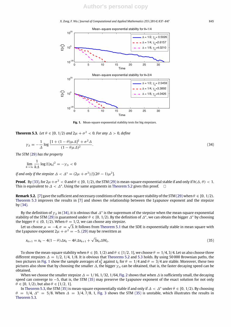
Fig. 1. Mean-square exponential stability tests for big stepsizes.

Theorem 5.3. Let θ ∈ [0, 1/2) and 2µ + σ 2 < 0. For any ∆ > 0, define

γ∆ = −1∆

log[1 + (1 − θ)µ∆]

2+ σ 2∆

(1 − θµ∆)2. (34)

The STM (29) has the property

limk→∞

1k∆

logE|xk|2 = −γ∆ < 0

if and only if the stepsize ∆ < ∆∗= (2µ + σ 2)/[(2θ − 1)µ2

].

Proof. By (33), for 2µ+σ 2 < 0 and θ ∈ [0, 1/2), the STM (29) is mean-square exponential stable if and only if h(∆, θ) < 1.This is equivalent to ∆ < ∆∗. Using the same arguments in Theorem 5.2 gives this proof.

Remark 5.2. [7] gave the sufficient andnecessary conditions of themean-square stability of the STM (29)when θ ∈ [0, 1/2).Theorem 5.3 improves the results in [7] and shows the relationship between the Lyapunov exponent and the stepsizeby (34).

By the definition of γ∆ in (34), it is obvious that ∆∗ is the supremum of the stepsize when the mean-square exponentialstability of the STM (29) is guaranteed under θ ∈ [0, 1/2). By the definition of ∆∗, we can obtain the bigger ∆∗ by choosingthe bigger θ ∈ (0, 1/2). When θ = 1/2, we can choose any stepsize.

Let us choose µ = −4, σ =√3. It follows from Theorem 5.1 that the SDE is exponentially stable in mean square with

the Lyapunov exponent 2µ + σ 2= −5. (29) may be rewritten as

xk+1 = xk − 4(1 − θ)∆xk − 4θ∆xk+1 +√3xk∆Wk. (35)

To show themean-square stability when θ ∈ [0, 1/2) and θ ∈ [1/2, 1], we choose θ = 1/4, 3/4. Let us also choose threedifferent stepsizes ∆ = 1/2, 1/4, 1/8. It is obvious that Theorems 5.2 and 5.3 holds. By using 50000 Brownian paths, thetwo pictures in Fig. 1 show the sample averages of x2k against tk for θ = 1/4 and θ = 3/4 are stable. Moreover, these twopictures also show that by choosing the smaller ∆, the bigger γ∆ can be obtained, that is, the faster decaying speed can beobtained.

When we choose the smaller stepsize ∆ = 1/16, 1/32, 1/64, Fig. 2 shows that when ∆ is sufficiently small, the decayingspeed can converge to −5, that is, the STM (35) may preserve the Lyapunov exponent of the exact solution for not onlyθ ∈ [0, 1/2), but also θ ∈ [1/2, 1].

In Theorem 5.3, the STM (35) is mean-square exponentially stable if and only if ∆ < ∆∗ under θ ∈ [0, 1/2). By choosingθ = 1/4, ∆∗

= 5/8. When ∆ = 3/4, 7/8, 1, Fig. 3 shows the STM (35) is unstable, which illustrates the results inTheorem 5.3.

Author's personal copy

846 X. Zong, F. Wu / Journal of Computational and Applied Mathematics 255 (2014) 837–847

Fig. 2. Mean-square exponential stability tests for small stepsizes.

Fig. 3. Unstable tests.

References

[1] E. Hairer, G. Wanner, Solving Ordinary Differential Equations II, second ed., in: Stiff and Differential Algebraic Problems, Springer-Verlag, Berlin, 1996.[2] A.M. Stuart, A.R. Humphries, Dynamical Systems and Numerical Analysis, Cambridge University Press, Cambridge, UK, 1996.[3] C.T.H. Baker, E. Buckwar, Exponential stability in p-th mean of solutions, and of convergent Euler-type solutions, of stochastic delay differential

equations, J. Comput. Appl. Math. 184 (2005) 404–427.[4] A. Bryden, D.J. Higham, On the boundedness of asymptotic stability regions for the stochastic theta method, BIT 43 (2003) 1–6.[5] K. Burrage, T. Tian, A note on the stability properties of the Euler methods for solving stochastic differential equations, New Zealand J. Math. 29 (2000)

115–127.[6] D.J. Higham, P.E. Kloeden, Numerical methods for nonlinear stochastic differential equations with jumps, Numer. Math. 101 (2005) 10–119.[7] D.J. Higham, X. Mao, C. Yuan, Almost sure and moment exponential stability in the numerial simulation of stochastic differential equations, SIAM J.

Numer. Anal. 45 (2007) 592–609.[8] Y. Saito, T. Mitsui, T -stability of numerical scheme for stochastic differential equations, in: Contributions in Numerical Mathematics, in: World Sci.

Ser. Appl. Anal., vol. 2, World Scientific, River Edge. NJ, 1993, pp. 333–344.[9] Y. Saito, T. Mitsui, Stability analysis of numerical schemes for stochastic differential equations, SIAM J. Numer. Anal. 33 (1996) 2254–2267.

[10] X. Mao, Stochastic Differential Equations and Applications, Horwood, Chichester, UK, 1997.[11] E. Buckwar, C. Kelly, Towards a systematic linear stability analysis of numerical methods for systems of stochastic diffeential equations, SIAM J. Numer

Math. 48 (2010) 298–321.[12] D.J. Higham, Mean-square and asymptotic stability of the stochastic theta method, SIAM J. Numer. Anal. 38 (2000) 753–769.[13] D.J. Higham, X. Mao, A.M. Stuart, Exponential mean square stability of numerical solution to stochastic differential equations, LMS J. Comput. Math. 6

(2003) 297–313.

Author's personal copy

X. Zong, F. Wu / Journal of Computational and Applied Mathematics 255 (2014) 837–847 847

[14] H. Schurz, V.L. Girko, Almost sure asymptotic stability and convergence of stochastic theta methods applied to systems of linear SDEs in Rd , RandomOper. Stoch. Equ. 19 (2011) 111–129.

[15] Y. Saito, T. Mitsui, Mean-square stability of numerical schemes for stochastic differential systems, Vietnam J. Math. 30 (2002) 551–560.[16] C. Huang, Exponential mean square stability of numerical methods for systems of stochastic differential equations, J. Comput. Appl. Math. (2012).

http://dx.doi.org/10.1016/j.cam.2012.03.005.[17] H. Szpruch, X. Mao, Strong convergence of numerical methods for nonlinear stochastic differential equations under monotone conditions, Technical

Report, Preprint, 2010.[18] L. Chen, F. Wu, Almost sure exponential stability of the θ-method for stochastic differential equations, Statist. Probab. Lett. 82 (2012) 1669–1676.[19] X. Mao, Exponential Stability of Stochastic Differential Equations, Marcel Dekker, New York, 1994.[20] F. Wu, X. Mao, L. Szpruch, Almost sure exponential stability of numeriacal solutions for stochastic differential delay equations, Numer. Math. 115

(2010) 689–697.[21] W. Wang, L. Wen, S. Li, Nonlinear stability of θ-methods for neutral differential equations in Banach space, Appl. Math. Comput. 198 (2008) 742–753.