Munich Personal RePEc Archive Child Malnutrition in India Vani Borooah May 2018 Online at https://mpra.ub.uni-muenchen.de/90550/ MPRA Paper No. 90550, posted 16 December 2018 03:49 UTC brought to you by CORE View metadata, citation and similar papers at core.ac.uk provided by Munich Personal RePEc Archive

Welcome message from author
This document is posted to help you gain knowledge. Please leave a comment to let me know what you think about it! Share it to your friends and learn new things together.
Transcript
MPRAMunich Personal RePEc Archive
Child Malnutrition in India
Vani Borooah
May 2018
Online at https://mpra.ub.uni-muenchen.de/90550/MPRA Paper No. 90550, posted 16 December 2018 03:49 UTC
brought to you by COREView metadata, citation and similar papers at core.ac.uk
provided by Munich Personal RePEc Archive
1
Chapter 4: Child Malnutrition in India
4.1. Introduction
Speaking in January 2012, on the occasion of the launch of the Naandi Foundation ‘s (2011)
report Hunger and Malnutrition (HUNGaMA), 1 the then Prime Minister, Manmohan Singh declared
that “the problem of malnutrition is a matter of national shame. Despite impressive growth in our
GDP, the level of malnutrition in the country is unacceptably high” (Government of India, 2011). The
HUNGaMA Report showed that, on the basis of a survey of 100 districts ranked lowest on the basis of
a child development index developed for the UNICEF, 42% of under-five children were underweight
and the 59% were stunted. The poignancy of these malnutrition figures lay in the fact that, despite
India’s remarkable growth, the basic needs of several children, involving inter alia access to food and
health care, were not being met. Therein lay the “national shame” which Prime Minister Singh
referred to: despite the fact that India was far more prosperous than several countries of Africa, its
rates of child malnutrition were considerably higher. For example, the percentage of under-5 children
who were stunted - that is, those children whose height-for-age was two standard deviations (2SD)
below World Health Organisation (WHO) norms - and underweight - that is, those children whose
weight-for-age was 2SD below WHO norms – was, for the period 2000-2009, respectively, 47.9%
and 43.5% in India compared to, respectively, 44.8% and 33.9% in Chad and 44.6% and 21.8% in the
Central African Republic (the latter being two of the poorest countries in Africa). 2
Panagariya (2013), however, drew attention to the fact that on every health indicator, other
than malnutrition, children in India fared better than their counterparts in Chad and the CAR with both
infant mortality (50 per 1,000 live births in India, compared to 124 in Chad and 112 in the CAR) and
under-five mortality (66 per 1,000 live births in India, compared to 209 in Chad and 171 in the CAR)
being lower in India. This better health performance also extended to adults – both life expectancy (65
years compared to 48 years in the Chad and the CAR) and maternal mortality (23 per 1, 000 live
1 Hungama is a Hindi word meaning ‘uproar’. 2 WHO (2011).
2
births in India, compared to 1,20 in Chad and 85 in the CAR) were, respectively, higher and lower in
India.3
In the face of these contradictions, and counter to the “national shame” perspective on child
malnutrition in India, Panagariya (2013) took the view that the high rate of child malnutrition in India
was the spurious artefact of measuring the nutritional status of Indian children, who were genetically
smaller than children in other nations, using unrealistically high WHO norms. Since 2006, these
norms are based, on a reference sample of 8,440 healthy breast-fed infants and young children -
drawn from Brazil, Ghana, India, Norway, Oman, and the USA - and the conclusion that
“approximately half of Indian children are malnourished are based on an application of these
standards” (Panagariya, 2013, p.103).
The average height of Indian males and females – respectively, 164.7 cm and 154.9 cm – is
lower than that of their counterparts in all the countries included in the WHO’s reference population
and so a “genetic bias” in applying over-ambitious norms to Indian children cannot be ruled out.4 On
the other hand, the average height of Sri Lankan males at females – respectively, 163.6 cm and 151.4
cm – is even lower than that for India but the proportion of Sri Lankan under-5 children that were
judged, on WHO norms, as stunted, in the period 2000-2009, was only 19.2% compared to India’s
47.9%.5 Similarly, the average height of Japanese men and women (respectively, 172 cm and 158
cm) is considerably lower than that of their Dutch counterparts (respectively, 181 cm and 169 cm)
but, judged by WHO norms, both countries are characterised by an almost complete absence of
stunting among under-five children.
So taking these facts into account, it is more likely that non-genetic factors, that are
independent of WHO norms, play a major role in determining stunting among children under five
years of age but, once children reach maturity, genetic factors – for example, the average, Japanese is
shorter than the average Dutchman – play a role in imposing different ceilings on the average heights
3 One needs, however, to be careful in comparing life expectancy in countries with different social conditions. For example, McCord and Freeman (1990) showed that black men in Harlem were less likely to reach the age of 65 than men in Bangladesh with the main causes of early mortality being homicide, cirrhosis, drug dependency, and alcohol. This argument is also relevant in comparing life expectancy in war-torn Chad and relatively peaceful India. 4 https://en.wikipedia.org/wiki/List_of_average_human_height_worldwide (accessed 30 November 2017). 5 WHO (2011).
3
of persons in different countries. This, in turn, raises two questions. First, in addition to non-genetic
factors, might genetic factors also play a role in producing underweight and stunted children? Second,
might differences in heights between different populations disappear as better nutrition allows shorter
populations to “catch-up”, perhaps over several generations, with their taller counterparts? The
evidence, as regards, the first question, is mixed. In support of the “genetic hypothesis”, Alexander et.
al. (2007) argued, for the USA, that ceteris paribus children born to resident Asian-Indian mothers
were more likely to be underweight than children born to white mothers. On the hand, finding against
the genetic hypothesis, Tarozzi (2008), in a comparison of children born to Indian mothers settled in
the UK with that of children from the reference population used to construct the WHO’s 2006 norms
argued that the growth performance of the former was comparable to that of the latter. The answer to
the second question is beyond the scope of this chapter but a good account of whether there is “catch-
up” in heights is provided by Bilger (2004).
So what might be the non-genetic factors influencing child malnutrition? Coffey et. al.
(2013), in their reply to Panagriya (2013), were dismissive of his “genetic argument” for explaining
the relatively high child malnutrition rates observed in India because they claimed that it was an
argument arrived at by residual without the support of any concrete evidence: “if we cannot think of
anything else, it must be genetics” (Coffey et. al. 2013, p. 68).6 Instead, the authors placed emphasis
on poor sanitation in India, engendered in large part by the preference of Indians to defecate in public
(Coffey and Spears, 2017). 7 A consequence of poor sanitation is that Indian children grow up in a
poor health environment which makes them vulnerable to disease, especially diarrhoeal diseases,
impairing their capacity to absorb nutrients. So, on this perspective it is not just food availability that
produces malnutrition but rather the interaction of food availability and disease.
The connection between malnourishment and the “capacity to absorb nutrients” argument has
also been made by Osmani and Sen (2003) but in the context of gender inequality Their basic message
is that the neglect of woman in patriarchal societies in terms of nutrition and healthcare means that,
6 Though it should be pointed out that one of the authors of this paper has also used the “genetics” argument”: “given that Africans are deprived in almost all dimensions, yet are taller than less-deprived people elsewhere it is difficult not to speculate about the importance of possible genetic differences in population heights [emphasis added]” (Deaton, 2007, p. 132-136). 7 The demand for toilets in India was extensively discussed in Chapter 2.
4
being under-nourished themselves, they often cannot provide sufficient nourishment to their foetuses
– male or female- leading to the phenomenon of “foetal malnourishment” – children are
undernourished while in the womb. For poorer families, in utero undernourishment buttresses the
disease and poverty engendered post-birth malnourishment of children. For richer families, in utero
undernourishment leads, as Barker (1998) argued, to a new regime of diseases like diabetes and
cardiovascular ailments.
Against this background of these two competing narratives of child malnourishment in India,
and excellent account of which is provided by Nisbett (2017), this chapter examines the relative
strengths of the determinants of child malnutrition in India paying attention to household
characteristics (social group, consumption level, education, location) and the characteristics of the
households’ dwellings (presence of toilets, separate kitchen, vent in the cooking area). The analysis
also examines the importance of anganwadis in combating child malnutrition through growth
monitoring, health checks, and the provision of supplementary food. In addition, a unique
characteristic of this study is that it draws attention to the importance of personal hygiene, through
washing hands with soap and water after defecation, as a prophylactic against diarrhoeal disease. As
the Naandi Foundation’s (2011) report observed, only 11% of mothers washed their hands with soap
after defecating and only 10% washed their hands with soap before feeding their child. The
transmission of germs through unwashed hands is likely, therefore, to be an important cause of
disease and, indeed, as this chapter shows, of greater importance than poor sanitation engendered by
an absence of toilets.
The results reported in this chapter are from the India Human Development Survey (hereafter,
IHDS-2011) which relates to the period 2011-12.8 This is a nationally representative, multi-topic
panel survey of 42,152 households in 384 districts, 1420 villages and 1042 urban neighbourhoods
across India. Each household in the IHDS-2011 was the subject of two hour-long interviews. These
interviews covered inter alia issues of: health, education, employment, economic status, marriage,
fertility, gender relations, and social capital. The IHDS-2011, like its predecessors for 2005 and 1994,
was designed to complement existing Indian surveys by bringing together a wide range of topics in a 8 Desai et. al.(2015).
5
single survey which made possible the analysis of associations across a range of social and economic
conditions.
A unique feature of the IHDS-2011 is that investigators measured the height (or length in the
case of infants) and weight of all children between 0 and 59 months of age (hereafter, simply
“children”) with a first measurement being followed by a corroborative second measurement. In the
results reported in this chapter, the height and weight of a child was computed as the average of the
relevant first and second measurements and it is these heights and weights of children that form the
basis for the results reported in this chapter.
In analysing these data, this study employs a genre which uses cut-off points to categorise
children (for example, as: ‘severely’, ‘moderately’, ‘not’, severely stunted) and then employs methods
of discrete choice estimation to explain the probabilities of children being in the different categories.
These studies are referred to as "category based" studies: Brennan et. al. (2004), who studied stunting
among children in the Indian states of Karnataka and Uttar Pradesh, is a recent example. The use of
discrete choice estimation methods - for example, logit, ordered logit, and multinomial logit - is
usually justified by arguing that the values of the variable underlying the categories are unobservable:
only the categories in which the different individuals find themselves are observed. The dependent
variable is treated as taking discrete values, because the variable underpinning these values is a
"latent" (or unobserved) variable.
The alternative to ‘category based’ studies is ‘person based’ studies. In the context of
empirical studies of malnutrition, Thomas et. al. (1991) studied the relation between maternal
education and the height of children in Brazil; Sandiford et. al. (1995) studied the interaction between
maternal literacy and access to health services in affecting the health of children in Nicaragua; Lavy
et. al. (1996) examined the relation, for Ghana, between the quality and accessibility of health care,
and child survival and child health outcomes; Thomas et. al. (1996) examined, for the Côte d’Ivoire
the impact of public policies on child height, child height for weight and adult BMI; Gibson (2001),
measured the size of the intra-household externality, arising from the presence of literate members in
the household, on height for age outcomes for children in Papua New Guinea; and Sahn and Stifel
(2002b) tested whether the gender impact on the nutrition of pre-school age children in Africa was

6
different for mother's schooling compared to father's schooling. However, results from ‘person based’
studies are more difficult to interpret in terms of conventional views of malnutrition (stunted/normal
stature; underweight/normal weight) and, so, the category-based approach was preferred.
4.2. A Preliminary Look at the Data
A child’s height-for-age is an indicator of ‘stunting’ which is a common manifestation of
malnutrition in children in developing countries. Other anthropometric measures employed to assess
malnutrition among children are weight-for-age for assessing the prevalence of under-weight children,
and weight-for-height for assessing the prevalence of 'wasting'. 9 A standard classification is to regard
a child as severely stunted if his/her (gender specific) height-for-age (HfA) was three standard
deviations (SD) below, and as stunted if the HfA was between two and three SD below the World
Health Organisation (WHO) norm for a child of that gender and that age. A child that was not stunted
is referred to in this chapter as being of normal stature. Similarly, the usual practice is to regard a
child as severely underweight if his/her (gender specific) weight-for-age (WfA) was three SD below,
and as underweight if his/her WfA was between two and three SD below the WHO norm for a child
of that gender and that age. At the other of the scale, this study classified a child as severely
overweight if his/her WfA was three SD above, and as overweight if his/her WfA was between two
and three SD above, the WHO norm for a child of that gender and age. A child whose WfA was
between ±2SD of the WHO norm is regarded as being of normal weight.10
Although child malnutrition in India has been commented upon extensively, there is less
evidence on how such malnutrition varies by social group. In order to address this issue, the IHDS-
2011 sample of households was subdivided according to their caste/religion: Brahmins (5% of
households); Forward Caste Hindus (FCH: 15% of households); non-Muslims from the Other
Backward Classes (OBC: 36% of households), Scheduled Castes (SC: 22% of households); Scheduled
9 However, unlike these measures, height-for-age is less affected by acute periods of stress at the time of measurement. Sahn and Stifel (2002a) point out that an acute episode of diarrhoea or malaria will not affect height-for-age. 10 The WHO standards may be obtained from http://www.who.int/childgrowth/standards/height_for_age/en/

7
Tribes (ST: 8% of households); Muslims (13% of households); and an ‘Other’ category comprising
Christians, Sikhs, and Jains (2% of households).11
<Table 4.1>
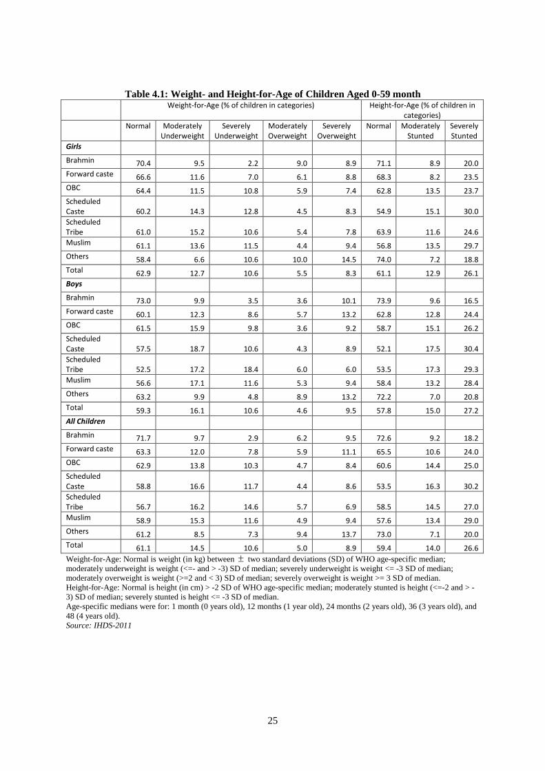
Table 4.1 shows variations in rates of being underweight and of stunting by social group.
Overall, 25.1% of all children in the sample were underweight (14.5% moderately underweight and
10.6% severely underweight) and 40.6% of all children were stunted (14% were moderately stunted
and 26.6% were severely stunted). This rate varied by gender – 26.7% of boys, compared to 23.3% of
girls were underweight while 42.2% of boys, compared to 39% of girls, were stunted – and also by
social group. In terms of the latter, Brahmin children had the lowest rates of being underweight and
stunted – 10.6% of them were underweight and 27.4% were stunted – while SC, ST, and Muslim
children had the highest rates of being underweight and stunted – respectively, 28.3%, 30.8%, and
26.9% of SC, ST, and Muslim children were underweight and respectively, 46.5%, 41.5%, and 42.4%
of SC, ST, and Muslim children were stunted.
A feature of nutrition studies for India is that they pay little attention to the phenomenon of
overweight children. Table 4.1 sheds light on this relatively neglected feature and shows that nearly
14% of all children were overweight with nearly 9% of all children being severely overweight.
Although there did there did not appear to be any gender disparity associated with being overweight,
there were marked differences between the social groups in terms of overweight children: on this
occasion, the highest rates of being overweight were associated with Brahmin and FCH children, and
children from the ‘Other’ group (comprising Christians, Sikhs, and Jains): respectively, 15.7%, 17%,
and 23.1% of children from these three groups were overweight, either moderately or severely.
Perhaps, unsurprisingly, the lowest rates of being overweight were associated with SC, ST, OBC, and
Muslim children: respectively, 13%, 12.6%, 13.1%, and 14.3% of children from these four groups
were overweight, either moderately or severely.
Measuring Inequality in the Inter-Group Distribution of Underweight and Stunted Children
11 All the figures reported in this chapter have been grossed up using the household weights provided by the IHDS-2011.
8
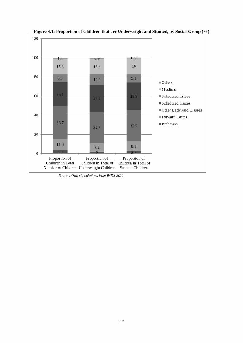
Figures 4.1 and 4.2 highlight the disproportionality between the representation of households
from the different households in the entire sample and their representation among those that had
underweight and stunted children.12 For example, Figure 4.1 shows that 3.9% percent of the total of
children whose heights and weights were recorded was Brahmin but these children comprised only
2% of all underweight children and only 2.7% of all stunted children. On the other hand, 25% percent
of the total of children whose heights and weights were recorded was from the SC but these children
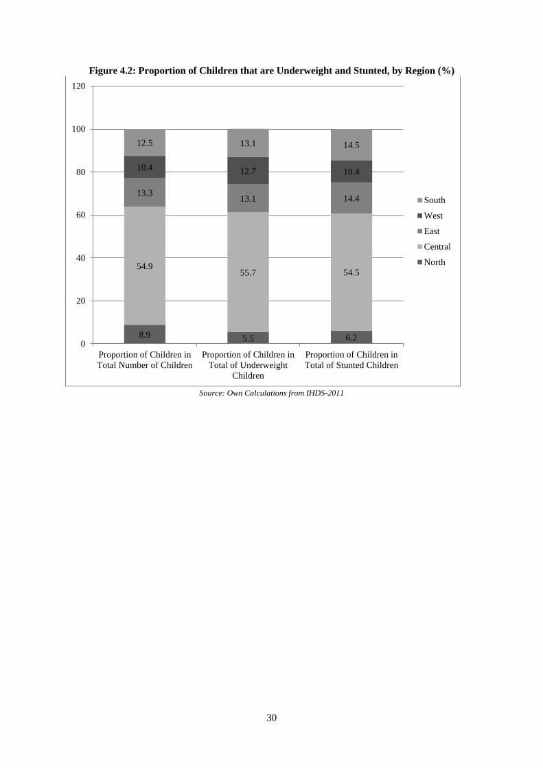
comprised 28% of all underweight children and 29% of all stunted children. In terms of the regions,
Figure 4.2 shows that 8.9% percent of the total of children whose heights and weights were recorded
lived in the North but these children comprised only 5.5% of all underweight children and only 6% of
all stunted children; at the other extreme, 10.4% percent of the total of children whose heights and
weights were recorded lived in the West and 12.5% lived in the South but these children comprised,
respectively, 13% of all underweight children and 14.5% of all stunted children.
<Figures 4.1 and 4.2>
These inter-group disproportionalities raise the question of how to aggregate them into a
single measure of inequality in respect of the distribution of underweight/stunted children. A useful
way of measuring inequality in a variable is by the natural logarithm of the ratio of its arithmetic
mean to its geometric mean Bourguignon (1979) and Theil (1967). This idea translates very naturally,
from its usual application to income inequality, to measuring the degree of inequality in the
distribution of low weight and height. The variable of interest is the proportion of children from a
group that are underweight/stunted (respectively, the ‘underweight rate’ and the ‘stunting rate’) and it
is inequality in the distribution of these rates between children in the different groups that is sought to
be measured.
Suppose that the sample is divided into M mutually exclusive and collectively exhaustive
groups with Nm (m=1…M) children in each group such that Nm and Hm are the numbers of children
from each group in, respectively, the sample (the ‘reference population’) and the underweight/stunted
12 Note that, the two categories, underweight and severely underweight of Table 4.1, have been merged in Figures 4.1 and 4.2 into a single category, “underweight”; similarly, the two categories, stunted and severely stunted, have been merged into a single category, “stunted”.

9
sub-sample (‘outcome population’) . Then 1 1
and M M
m mm m
N N H H= =
= =∑ ∑ are, respectively, the total
numbers of children in the reference and the outcome population.
The underweight/stunting rate of children in group m (denoted um) is / , 0 1m m m mu H N u= ≤ ≤
. Then the arithmetic and geometric means of um are, respectively:
1 11
ˆ ( ) / , 1m
MM Mn
m m m m m mm mm
u u n and u u where n N N n= ==
= = = =∑ ∑∏ (4.1)
so that the measure of nutritional inequality is:
1
ˆlog( / ) log( ) - log( )M
m mm
J u u u n u=
= = ∑ (4.2)
Now from the definition of um:
( )( )( ) ( )/ / / / ( / )( / )( / ) /m m m m m m m m mu H N H N N H H N H H N N H N h n u= = = = (4.3)
where : / /m m m mh H H and n N N= = are, respectively, the share of children in group m in the total
of children (reference population) and in the total of children that are underweight/stunted (outcome
population). Employing equation (4.3) in equation (4.2) yields:
1 1 1
ˆlog( / ) log( ) log( ) log( ) log logM M M
m mm m m m
m m mm m
h hJ u u u n u u n u nn n= = =
= = − = − = −
∑ ∑ ∑ (4.4)
From equation (4.4), inequality is minimised when J=0. This occurs when m mn h= , that is
when the share of a group's children in the ‘reference population’ (nm) is equal to their share in the
‘outcome population’ (hm), J>0, otherwise. Inequality is maximised when only children from one
group, but none from the other groups, are underweight/stunted. If the underweight/stunted group is,
say, group 1, 1 2 31, ... 0mh h h h= = = = ). Then max 1 1 1 1log(1 / ) log( )J n n n n= − = and, therefore,
1 10 log( )J n n≤ ≤ .
Using the numbers shown in Figures 4.1 and 4.2 (for the nm and the hm of equation (4.4)) the
computed values of Jsocgroup were 1.6 for underweight and 0.57 for stunting while the computed values
of Jregion were 1.0 for underweight and 0.71 for stunting . The maximum value of Jsocgroup, under the
assumption that all (and only) SC children were underweight or stunted households was 80.9 and the
maximum value of Jregion, under the assumption that all (and only) Central region children were
10
underweight or stunted was 219.9. Thus the observed level of inter-group and inter-regional
inequality in children being underweight or stunted was very low: at the very largest, only 2% of the
maximum amounts of inequality. 13
4.3. Econometric Analysis: Specifying the Low Weight and Stunting Equation
Differences between the social groups in the proportion of their children that were
underweight or stunted, shown in Table 4.1, raise two questions. The first and obvious question is to
ask whether the numerical differences observed in Table 4.1 were statistical significant (in the sense
that the likelihood of observing these differences, under the null hypothesis of no difference, was
sufficiently small)? The second question follows from the observation that the children in the sample
differed in terms of more than just social group membership. For example, different children lived in
different regions of India; some resided in rural areas, others were urban residents; some had educated
parents while others had parents who entirely lacked education; some children lived in households
which enjoyed a high level of consumption, others came from poorer households. The second
question is, therefore, whether differences between social groups in the proportion of their children
that were underweight or stunted would survive after such factors had been controlled for?
This study focuses on the likelihood of a child being underweight or stunted after controlling
for a variety of factors relating to his/her circumstances. Under the aegis of such ‘category based’
analysis, discussed earlier, the dependent variable yi, defined over N children (indexed, i=1…N), was
assumed to take the value 1 if child i was underweight/stunted and 0 if it was not.14 In estimating the
logit model in the presence of an intercept term, it was not possible, for reasons of multicollinearity,
to include all the categories with respect to the variables; the category that was omitted for a variable
is referred to as the reference category (for that variable).
If Pr[yi=1] represents the probability of a child being underweight/stunted (so that
Pr[yi=0]=1- Pr[yi=1] represents the probability of not being underweight/stunted), the logit
13 Note, however, that the value for the maximum level of inequality depends crucially upon where the burden of low weight or stunting is assumed to be concentrated. 14 Where a child is regarded as underweight (stunted) if his/her WfA (HfA) is 2SD below the WHO norm. In other words, the two categories, underweight and severely underweight, have been merged into a single category, “underweight”; similarly, the two categories, stunted and severely stunted, have been merged into a single category, “stunted”.
11
formulation expresses the log of the odds ratio as a linear function of K variables (indexed k=1…K)
which take values, 1, 2 ...i i iKX X X with respect to child i, i=1…N:
1
Pr[ 1]log1 Pr[ 1]
Ki
k ik i iki
y X u Zy
β=
== + = − = ∑ (4.5)
where: βk is the coefficient associated with variable k, k=1…K.
From equation (4.5) it follows that:
ˆ
ˆ1
Pr[ 1]1
i i
i i
z X
i z X
e
e
eye
β
β+= = =
+ (4.6)
where, the term ‘e’, in the above equation represents the exponential term.
The variables used to explain the likelihood of children being underweight/stunted were
grouped as follows:
A. Mother’s Nutritional Status
It was likely that the mother’s nutritional status (whether she was underweight, of normal
weight, pre-obese, or overweight) would also influence the WfA and HfA of her children. This
reflects the view that the under-nourishment of children begins in the womb, with under-nourished
mothers giving birth to under-nourished babies (Osmani, 2001; Osmani and Sen, 2003).
Consequently, foetal under-nourishment might be expected to be greater for underweight mothers and
mothers in poor health. In order to accommodate this view, the BMI status of mothers (normal
weight; underweight; pre-obesity; and overweight) and the health status of mothers (good or very
good; ok or poor to very poor) were included among the determining variables.
B. Age Group of Children
It was also conceivable that the nutritional status of children could vary with age such that the
probability of being underweight or stunted increased or decreased with age. In order to allow for this,
children were grouped by age (0-1 years, 1-2 years, 2-3 years, 3-4 years, and 4-5 years) and these age
groups were included as determining variables of the likelihood of being underweight or stunted.
C. Gender
There is ample evidence that Indian parents have a marked preference for having sons over
daughters (Borooah and Iyer, 2005) and that this is reflected in the relative neglect of the girl child in
12
terms of diet and health care (Sen, 2001; Borooah, 2004). Consequently, one might expect a gender
bias to exist in terms of nutritional achievement and, so, the gender of a child was included among the
determining variables.
D. Social Group
As discussed earlier, these related to the social group, defined in terms of religion/caste, to
which the households belonged: Brahmins; Forward Caste Hindus (FCH); Hindus from the Other
Backward Classes (OBC), Scheduled Castes (SC); Scheduled Tribes (ST); Muslims; and an ‘Other’
category comprising Christians, Sikhs, and Jains.
E. Income and Education.
It might be expected that the likelihood of a child being malnourished (either by way of being
underweight or being stunted) would be influenced by its household’s standard of living. In order to
capture the “income effect” each household was placed in one of five quintiles of household per-
capita consumption expenditure (lowest, 2nd quintile, 3rd quintile, 4th quintile, highest quintile)
depending upon its reported expenditure.
It might also be expected that the higher the educational level of the adults in a child’s
household, the lower would be its likelihood of being malnourished since higher levels of education
could lead to greater awareness of the appropriate diet for children as well as of the importance of a
clean and disease free environment in which to raise children. The education level of a household was
measured by the highest level of education of an adult member. Five levels of education were
distinguished: (i) no education; (ii) up to primary level of schooling; (iii) above primary and up to
secondary level of schooling; (iv) higher secondary; (v) graduate or above.
F. Region
The incidence of malnourishment might also vary according to the exigencies of region.
Dietary norms might vary according to region with some regions emphasising a protein-rich diet
based on milk, meat, eggs, and fish while in other regions many of these items might be precluded
from the household diet on account of dietary restrictions.
In order to capture this regional dimension to child malnourishment this study aggregated the
Indian states into the following regions: North (comprising the states of Jammu & Kashmir, Delhi,
13
Haryana, Himachal Pradesh, Punjab (including Chandigarh), and Uttarakhand); the Centre (Bihar,
Chhattisgarh, Madhya Pradesh, Jharkhand, Rajasthan, and Uttar Pradesh); the East (Assam, Orissa,
West Bengal, and the North-Eastern states15); the West (Gujarat and Maharashtra); and the South
(Andhra Pradesh, Karnataka, Kerala, and Tamil Nadu).
G. Other Housing Amenities
It was also plausible that the environment of the dwelling in which a child was raised would
impact on his/her propensity to illness and, in consequence, through its inability to absorb nutrients,
on its likelihood of being malnourished. A healthy environment might be determined by amenities
within the dwelling such as: (i) having a toilet; (ii) a separate kitchen; (iii) a vent in the cooking area;
(iv) pucca roof and floor16; (v) electricity; (vi) water supply within the house or its compound.
H. Anganwadi Benefits
Chapter 3 referred to the government of India’s Integrated Child Development Services
(ICDS) Program which is its largest national program for promoting the health and development of
mothers and their children. The scheme is targeted at children below the age of 6 years and their
mothers (particularly if they are pregnant and lactating) and benefits take the form of inter alia
supplementary nutrition, immunisation, regular health checks, referral services, education on nutrition
and health, and pre-school learning. In addition, mothers and children are provided with iron, folic
acid, vitamin A tablets to combat, respectively, iron deficiency, anaemia, and xerophthalmia. The
scheme – which is based on the principle that the overall impact of these benefits would be greater if
they were provided in an integrated manner rather than on a piecemeal basis - is administered from a
centre, called the anganwadi (meaning village courtyard), by workers and their helpers, trained and
paid an honorarium under the scheme (Kapil and Pradhan, 1999). Over 58 million children, aged 0-6
years, were covered by this scheme in 2006-07 and this was expected to rise to over 72 million in
2008-09 (Diwakar, 2010).
Consequently, it might be expected that specific aspects of anganwadi activities, where they
related to nutrition and health, might be expected to reduce the incidence of underweight and stunted
15 Sikkim, Arunachal Pradesh, Nagaland, Mizoram, Manipur, Tripura, Meghalaya. 16 A pucca roof was made asbestos, metal, brick, stone, concrete. A pucca floor was one not made of mud or wood.
14
children. From the plethora of anganwadi activities, three were chosen in this study for econometric
investigation: whether a child’s mother had used an anganwadi to (i) have his/her growth monitored;
(ii) have his/her health checked; (iii) to obtain supplementary food for the child.
I. Personal Hygiene
The IHDS-2011 gave information on the post-defecation handwashing habits of households
both in terms of whether household members washed their hands (never, sometimes, usually, always)
and in terms of what they washed their hands with (water only, mud or ash, soap). There is
compelling evidence that there is a strong association between the hand-washing habits of household
adults, in particular of mothers, and likelihood of children in the household being afflicted by
diarrhoeal illness (Borooah, 2004; Huang and Zhou, 2007, Ejemot-Nwadiaro et. al., 2015 ).17 Given
that diarrhoea accounts for 1.8 million deaths in children in low and middle income countries it is
important to examine the influence of hand washing practices on child malnutrition.
In order to capture this aspect, data from the IHDS-2011 was used to construct a variable hi,
indexed i=1…N, such that hi =1 if members of a child’s household usually or always washed their
hands with soap after defecating and hi =0, otherwise.18 The IHDS-2011 showed, after grossing up
using the survey’s sample weights for households, that the variable hi took the value 1 (usually/always
washed with soap) for 85% of Brahmin households, 80.8% of FC households, 60.8% of OBC
households, 56.5% of SC households, 42.5% of ST households, 68.3% of Muslim households, and
88.4% of ‘other’ households.
4.4 Estimation Results
Following the advice contained in Long and Freese (2014), the results from the estimated
logit equation are presented in Tables 4.2 and 4.3 in the form of predicted probabilities from the
estimated logit coefficients (made possible by using a suite of options associated with the powerful
margin command in STATA v14.0) and not in terms of the estimates themselves.19 This is because
17 The vast majority of diarrhoeas are caused by infectious pathogens which reside in faeces and which employ a variety of routes to enter a new host. Since one such route is getting onto fingers and, thereby, into foods and fluids, the incidence of diarrhoea can be reduced by improvements in domestic hygiene. 18 hi=0 included households that always washed their hands but not with soap and also included households that usually washed their hands with soap. 19 These options, which are only available from STATA 13.0 onwards.
15
the logit estimates (represented by the vector β in equation (4.5)) do not have a natural interpretation –
they exist mainly as a basis for computing more meaningful statistics and, in this case, these are the
predicted probabilities of equation (4.6). Tables 4.2 and 4.3 show, respectively, the values of the
predicted probabilities of being underweight (PPU) and the predicted probabilities of being stunted
(PPS), based on logit estimates on data for 6,764 children (underweight equation) and 7,827 children
(stunted equation) for each category of determining variable listed under A-I above. The values of
PPU and PPS were computed using the method of “recycled predictions”, described in chapter 2. This
method isolates the effect of the different categories of variables on the children’s predicted
probabilities of being underweight (PPU) or their predicted probabilities of being stunted (PPS).
So, for example, in terms of the social groups category, first “pretend” that all the children in
the estimation sample are Brahmin. Holding the values of the other variables constant (either to their
observed sample values, as in this chapter, or to their mean values), predict the probabilities of being
underweight for each child under this all-Brahmin scenario and denote the mean of these values by
Bp . Then Bp represents the predicted probability of being underweight (PPU) for Brahmin children.20
Next, “pretend” that all the children are Muslim and, again holding the values of the other variables
constant, predict the probabilities of being underweight for each child under this all-Muslim scenario
and denote the mean of these values by Mp . Then Mp represents the predicted probability of being
underweight (PPU) of Muslim children. 21
Since the values of the other variables were unchanged between these two hypothetical
scenarios, the only difference between them is that, in the first scenario, the Brahmin variable was
“switched on” (with the variables pertaining to the other groups “switched off”) for all households
while, in the other, again for all households, the Muslim variable is “switched on” (with the variables
pertaining to the other groups “switched off”).22 Consequently, the difference between Bp and Mp is
entirely due to differences between Brahmin and Muslim children without the interposition of any
other factors.
20 An identical exercise can be performed for (PPS), the predicted probability of being stunted. 21 An identical exercise can be performed for (PPS), the predicted probability of stunting. 22 In operational terms, STATA’s margin command will perform these calculations.
16
In essence, therefore, in evaluating the effect of two characteristics X and Y on the likelihood
of a particular outcome, the method of “recycled predictions” compares two outcomes: first, under an
“all have the characteristic X” scenario and, then, under an “all have the characteristic Y” scenario, the
values of the other variables unchanged between the scenarios. The difference between the two
probabilities could then be ascribed to the attribute represented by X and Y (in this case, Brahmin and
Muslim).23
<Tables 4.2 and 4.3>
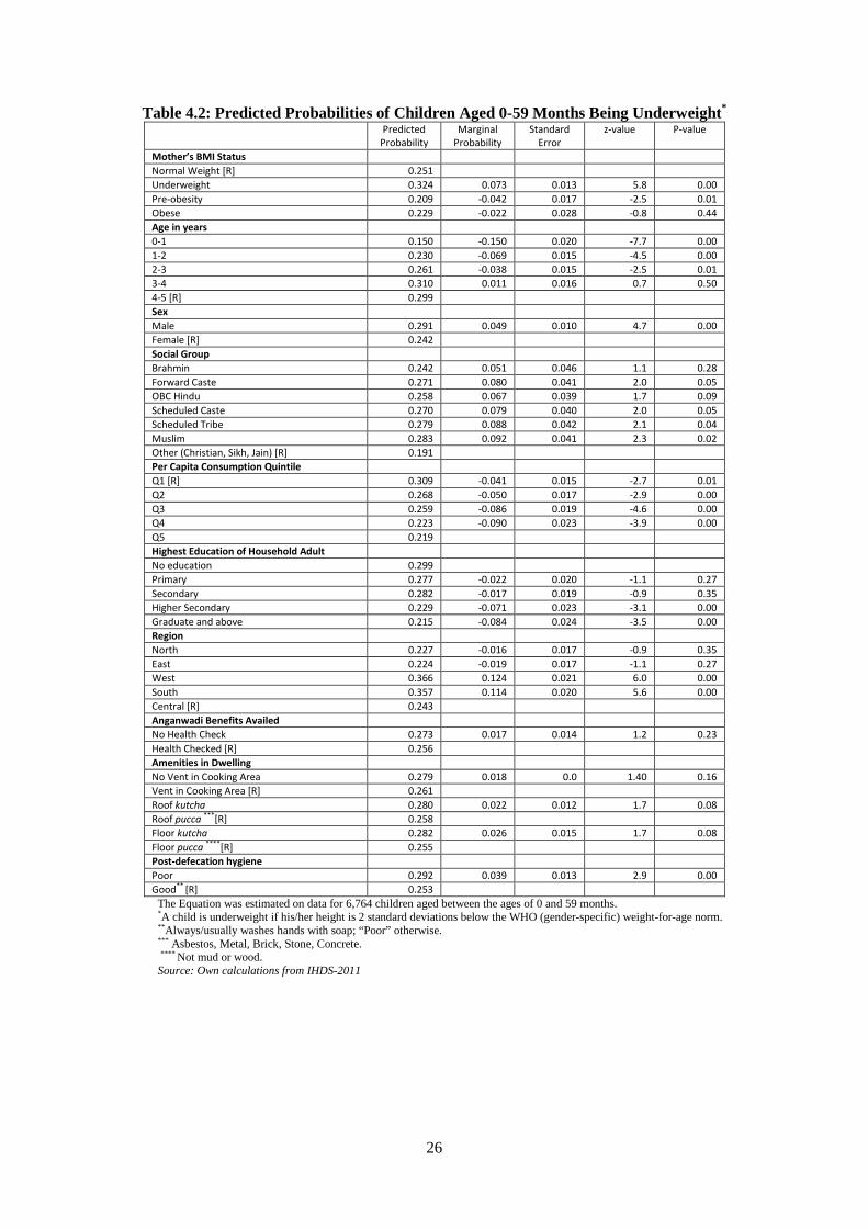
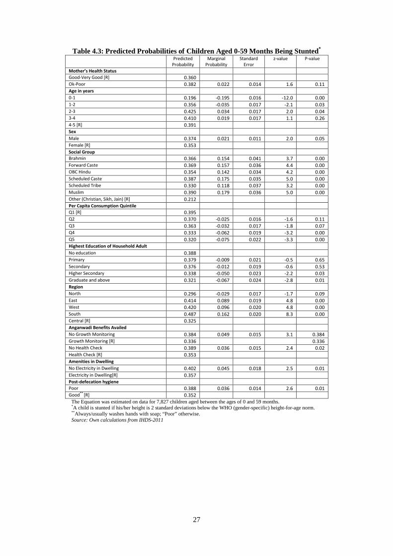
The second column of Tables 4.2 and 4.3, labelled ‘predicted probability’, show, respectively
the predicted probabilities of being underweight (PPU) and of being stunted (PPS) where these
probabilities were computed using the method of recycled predictions described above and, in more
detail, in chapter 2. Thus the number 0.242 in the predicted probability column and the Brahmin row
of Table 4.2 means that that if ceteris paribus all the 6,764 children in the estimation sample were
regarded as Brahmins then PPU=24.2%; similarly, the number 0.366 in the predicted probability
column and the Brahmin row of Table 4.3 means that that if ceteris paribus all the 7,827 children in
the estimation sample were regarded as Brahmins then PPS=36.6%. By contrast, for children in the
‘Other’ group, which was the reference group, the PPU and PPS were computed as 19.1% (Table 4.2)
and 21.2% (Table 4.3).
The marginal probabilities, shown in column 3 of Tables 4.2 and 4.3, represent, for every
variable category, the difference between the PPU and PPS of children in a specific group and
children in the reference group: so, from Table 4.2, the marginal probability of being underweight of
children aged 0-1 years, with children aged 4-5 as the reference group, was -19.5 points (19.6-39.1 =-
19.6 points) and, from Table 4.3, the marginal probability of boys being stunted, with girls as the
reference group, was 2.1 points (37.4-35.3 =2.1 points). Dividing these marginal probabilities by
their standard errors (column 4 of Tables 4.2 and 4.3) yielded the z-values (column 5 of Tables 4. 2
and 4.3); these z-values showed whether the marginal probabilities were significantly different from
23 For example, (i) X: all the children are Brahmin; Y: all the children are Muslim; (ii) X: all the children live in the North; Y: all the children live in the East.
17
zero in the sense that the likelihood of observing their values, under the null hypothesis of no
difference, was appreciably small (most usually, less than 5%).
The first feature of note in Tables 4.2 and 4.3 is the importance of the mother’s health in
determining the likelihood of a child being underweight or stunted. Table 4.2 shows that the average
likelihood of being underweight was significantly higher for children born to mothers whose Body
Mass Index (BMI) classed them as underweight than to mothers with a “normal” BMI: 32.4% versus
25.1%.24 Table 4.3 suggests that the average likelihood of being stunted was significantly higher for
children born to mothers whose self-perceived health status was “poor” compared to mothers whose
self-perceived health status was “good”: 38.2% versus 36.0%.
A second notable feature is the fact that good hygiene – meaning that members of a
household always/usually washed their hands with soap after defecation – played an important role in
determining the likelihood of a child being underweight or stunted. Compared to the average
likelihood of children, from households where hygiene was good, being underweight or stunted
(respectively, 25.3% and 35.2%), the average likelihood of children, from households where hygiene
was poor, being underweight or stunted (respectively, 29.2% and 38.8 %) was significantly higher.25
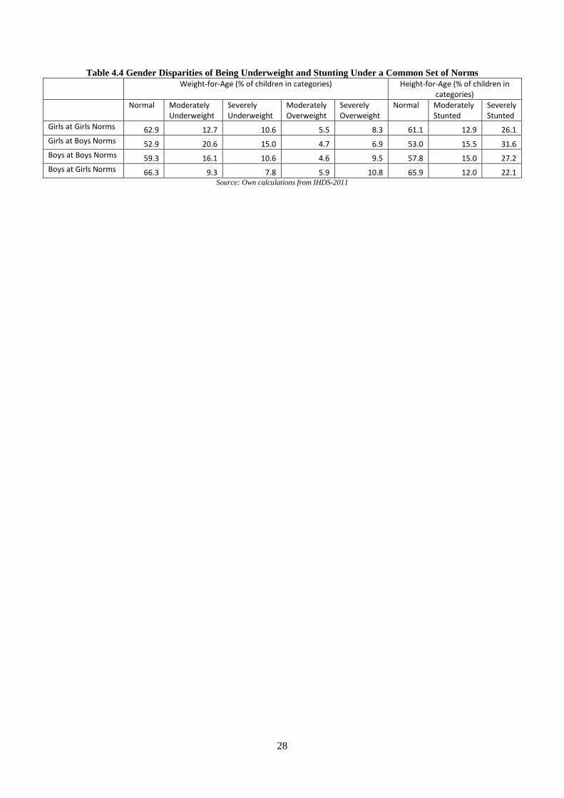
<Table 4.4>
The fourth feature of note was that girls were, on average less likely to be underweight or
stunted than boys: 24.2% versus 29.1% for being underweight and 35.3% versus 37.4% for stunting.
This differential in favour of girls can be entirely accounted for by the fact that the WHO norms for
weight-for-age and for height-for-age were lower for girls than for boys. Recalculating the rates of
girls and boys, aged 0-59 months, being underweight and stunted, if each gender’s weight-for-age and
height-for-age had been evaluated using the norms for the opposite gender, shows (Table 4.4) that the
underweight and stunting rate for girls, evaluated at boys’ rates, would have been higher than that for
boys while the underweight and stunting rate for boys, evaluated at girls’ rates, would have been
lower than that for girls.
24 The BMI is calculated as weight in kilograms divided by the square of the height in metres. A BMI below 18.5 places a person as “underweight, a BMI between 18.5 and 24.9 class a person as normal, a BMI between 25.0 and 29.9 indicates pre-obesity, while a BMI above 30.0 suggests obesity. 25 Poor if, post-defecation, household members did not always/usually wash hands with soap.
18
Tables 4.2 and 4.3 also show that rates of being underweight and stunted fell as the quintile of
children’s household per-capita consumption rose. Only 21.9% and 32% of children whose
households were in the highest quintile were, respectively, underweight and stunted compared to
30.9% and 39.5% of children whose households were in the lowest quintile. Similarly, tables 4.2 and
4.3 also show that rates of being underweight and stunted fell for children in households with higher
levels of adult education: only 21.5% and 32.1% of children from households, in which at least one
adult was a graduate, were, respectively, underweight and stunted compared to 29.9% and 38.8% of
children from households in which all adults were without any education.
There was some evidence that dwelling amenities affected the likelihood of being
underweight and stunted. Most notably, households without a pucca roof or floor were more likely to
have underweight children (Table 4.2) while households without electricity were more likely to have
stunted children (Table 4.3). Several anganwadi benefits alleviated the conditions of being
underweight or stunted. There was some weak evidence that the likelihood of being underweight was
lower for children whose mothers utilised anganwadi services for checking children’s health and there
was more compelling evidence that the likelihood of being stunted was lower for children whose
mothers utilised anganwadi services for checking children’s health and for monitoring children’s
growth.
In addition to these effects, there were strong regional effects. The likelihood of being
underweight was lowest in the North, the East, and the Centre (respectively, 22.7%, 22.4%, and
24.2%) and highest in the West and the South (respectively, 36.6% and 35.7%) with the likelihood of
being underweight significantly higher for children in the West and the South compared to children in
the (reference) Central region. Similarly, the likelihood of being stunted was lowest in the North and
the Centre (respectively, 29.6% and 32.5%) and highest in the East, West and the South (respectively,
41.4%, 42%, and 48.7%) with the likelihood of being stunted significantly higher for children in the
East, the West, and the South compared to children in the (reference) Central region.
The last point about the results reported in Tables 4.2 and 4.3 is that, even after controlling for
other variables, there were significant inter-social group differences in the likelihood of children being
underweight or stunted. Except for Brahmins, children from every other group (OBC, ST, SC,
19
Muslim) had a significantly higher likelihood of being underweight than children from the reference
group of ‘Others’ (Christians, Sikhs and Jains). Similarly, children from every other group (including
Brahmins) had a significantly higher likelihood of being stunted than children from the reference
group of ‘Others’. However, there was no significant difference between the non-reference groups
(Brahmin, OBC, SC, ST, and Muslim) in the predicted likelihood of their children being underweight
(PPU) or stunted (PPS).
Malnutrition of Children from “Elite” Households
Tarazzo (2008), using data from the National Family Health Survey for 1998/99 (NFHS2) for
children under three years of age, investigated what the rate of stunting and underweight would be for
children living in “elite” households - defined as those “from urban areas, where both parents have at
least a high school diploma, live in a house with a flush toilet, with a separate room used as a kitchen,
and whose family owns a car, colour television, telephone and refrigerator” (p. 463) – and concluded
that, applying WHO standards to these data, the rates of underweight and stunting in these
households would be, respectively, 9.4% and 20%.
In a similar vein, this chapter examined the rate of underweight and stunting for children
under five years old living in “elite” households where now these are defined as: (i) from urban areas
(ii) in the North of India, (iii) where at least one household adult is an graduate, (iv) where the
household’s per-capita consumption expenditure places it in the highest quintile, (v) where the
household’s main source of income is from professional work or salaried employment, (vi) where the
household lives in a house with (a) a toilet, (b) with a separate room used as a kitchen, (c) with a vent,
with a (d) pucca roof and floor, with (e) electricity and (f) water sourced from within the dwelling
premises. Under these elite household circumstances, the predicted probability of children being
underweight was 12.9% (compared to 26.7% for children from all households) and the predicted
probability of children being stunted was 21.9% (compared to 36.4% for children from all
households).
These findings invite the worrying conclusion, noted by Panagariya (2013), that even if the
children in the IHDS-2011 lived in households which satisfied many of the parameters conducive to
good nutritional levels, approximately one in 10 would be underweight and one in five would be
20
stunted. This raises two possibilities. The first is that, à la Panagariya (2013), there are genetic
differences between Indian children and children from the reference WHO population so that using
WHO norms would overstate the amount of child malnutrition in India. The second is that, à la
Deaton and Dreze (2009), the Indian population is still “catching up” with the WHO reference
population and the fact that there is a substantial amount of underweight and stunting, even among
children living in households embodying the most favourable nutritional circumstances, means that
the process of “catch up” is still incomplete.
4.5 Conclusions
Svedberg (2000) referred to the five w's of malnutrition: what is malnutrition: who are the
malnourished? Where are the malnourished? When are people malnourished? And why are people
malnourished? In terms of these questions, this chapter, with its focus on children 0-5 years of age,
defined what is malnutrition, it identifies who the malnourished children were in terms of their
caste/religious group; it located where undernourished children live in terms of the Indian regions;
and it studied when and why children were malnourished by examining the relative strength of the
variables which influenced malnutrition and, lastly, it added a sixth question by asking whether there
was a caste bias/religious to the malnutrition of children in India?
Even though the incidence of malnutrition in India has improved greatly since
Independence,26 the prevalence of malnutrition in India is extremely high even relative to other poor
countries. In the 1990s, 36 % of children below the age of five, compared to 21 % in Sub-Saharan
Africa were 'severely stunted'; 49 % of women between the ages of 20-29 years in India, compared to
21 % in Sub-Saharan Africa had a Body Mass Index (BMI) of less than 18.5 (Svedberg, 2001). On
more recent data, the National Family Health Surveys report that between 1998-99 and 2005-06 there
was virtually no improvement in children’s weights so that even today India has the highest
proportion of undernourished children than almost any other counter in the world: the UN reports for
2012 that 43% of Indian children were ‘underweight’ and 48% were ‘severely stunted’ compared to
26 See Dreze and Sen (2013)
21
21% and 40% for Sub-Saharan Africa, and 33% and 39% for South Asia, in their entirety.27 That
said, WHO (2017) reported that the rate of stunting for under-five children fell to 38.1% over 2005-16
from 47.9% over 2000-09 (as reported in WHO, 2011).
It is, however, more difficult to arrive at a universally acceptable explanation for which the
measured amount of child malnutrition should be so high. The explanation most commonly provided
is that of a hostile health environment centring on poor sanitation engendered, in turn, by the
preference of Indians for defecating in the open. On this explanation, if rates of open defecation in
India fell (to say, sub-Saharan levels or to levels in neighbouring Bangladesh) then there would be
concomitant fall in rates of malnourishment. In putting forward this argument, much is made of the
role of ‘untouchability’ among Hindus and the religious divide between upper-caste Hindus, who, for
reasons of religious purity, have a preference for defecating in the open and Muslims who have a
greater propensity to use toilets. As chapter 2 showed, while this an entertaining hypothesis, and one
that chimes with western views of Indian society, the evidence for it is little more than anecdotal and
the hypothesis does not survive a rigorous analysis of the data.
The second explanation is that, in nutritional terms, India is in a catch-up phase and that, just
as Germans and the Dutch became taller over time (Bilger, 2004) so too will Indians - but it will take
time.28 On this argument, converting a malign food/health environment into a benign one would
reduce the incidence of stunting and underweight but, even after this was achieved, it would still mean
that a substantial proportion of Indian children would remain malnourished. This is the explanation
provided for the fact that rates of underweight or stunting in India are high even among children from
“elite” households.
The third explanation is genetic: Indians are genetically smaller that several others of the
world’s populations and that, therefore evaluations based on norms based on reference population
drawn from various countries in the world will create an impression of malnourishment where none
might exist. However, the weight of academic opinion is that height variations within a population
are largely genetic (Ram is taller than Raj because his parents are taller) but that height differences
27 See UN data, http://data.un.org/Data.aspx?d=SOWC&f=inID%3a220 (for underweight) and http://data.un.org/Data.aspx?d=SOWC&f=inID%3A106 (for stunting). 28 For example, according to Bilger (2004), Americans haven’t grown taller in fifty years.
22
between populations are a kind of biological shorthand reflecting a composite of the factors that go
towards determining a society’s well-being (Bilger, 2004).
The fourth explanation, to which less attention is paid, is the treatment of women. Gender
discrimination means that women are more likely to be under-nourished than men. For example, the
IHDS-2011, shows that 26% of married women lived in families in which the men ate first. The
under-nourishment of women is not just a matter of reductions in the amount of food but also
deficiency in terms of micro-nutrients. One of the most important of these is deficiencies is iron
deficiency which in turns causes anaemia. As Ramachandran (2014) notes, iron deficiency anaemia is
particularly endemic in India with Bangladesh (36%) ranking higher than India (51%) in terms of the
proportion of women of child-bearing age who are anaemic.29 More worryingly, the prevalence of
anaemia among expectant mothers in India is nearly 70% (Ramachandran, 2014, p. 135). Adverse
consequences of child birth by anaemic mothers include intrauterine growth retardation, pre-maturity
and low birth weight, all with significant mortality risks, particularly in the developing world with
iron deficiency during the first trimester having a more negative impact on foetal growth than anaemia
developing later in pregnancy (Abu-Ouf and Jan, 2015).
Sen (2001) asks the very relevant question of how can things be changed? Although India
has made great strides in agricultural production and technology since Independence, “the false belief
that India has managed the challenge of hunger very well since independence is based on a profound
confusion between famine prevention, which is a simple achievement, and the avoidance of endemic
undernourishment and hunger, which is a much more complex task” (Sen, 2001, p.1). India has done
worse than nearly every country in the world in the latter respect but what is the real cause for anxiety
is the "silence with which it is tolerated, not to mention the smugness with which it is sometimes
dismissed" (Sen, 2001, p.1).
29 The problem is exacerbated by predominantly vegetarian diet in India (Ramachandran, 2014, p.129).
23
References
Abu-Ouf, N.M. and Jan, M.M. (2015), “The Impact of Maternal Iron Deficiency and Iron
Deficiency Anaemia on Child’s Health”, Saudi Medical Journal, 36 (2): 146-49.
Alexander, G.R., Wingate, M.S., Mor, J., and Boulet, S. (2007), “Birth Outcomes of Asian
Indian Americans”, International Journal of Gynaecology and Obstetrics, 97: 215-20.
Barker, D.J.P. (1998), Mothers, Babies and Diseases in Later Life, Churchill Livingstone:
London.
Bilger, B. (2004), “The Height Gap”, New Yorker, 5 April: 1-11.
Brennan, L., McDonald, J., Shlomowitz, R. (2004), “Infant feeding practices and chronic
child malnutrition in the Indian states of Karnataka and Uttar Pradesh”, Economics and Human
Biology 2: 138-158.
Coffey, D., Deaton, A., Dreze, J., Spears, D., and Tarozzi, A. (2013), “Stunting Among
Children: Facts and Implications”, Economic and Political Weekly, 68: 68-70.
Coffey, D. and Spears, D. (2017), Where India Goes: Abandoned Toilets, Stunted
Development and the Costs of Caste, Harper Collins Publishers India: Noida, Uttar Pradesh.
Deaton, A. (2007), “Height, Health, and Development”, Proceedings of the National
Academies of Science, 104 (33): 13232-37.
Deaton, a. and Dreze, J. (2009), “Food and Nutrition in India: Facts and Interpretation”,
Economic and Political Weekly, 44: 42-65.
Government of India (2012), “PM’s Speech at the Release of HUNGaMA (Hunger and
Malnutrition) Report”, Press Release, Press Information Bureau, Prime Minister’s Office, 10th
January, http://pib.nic.in/newsite/PrintRelease.aspx?relid=79457 (accessed 29 November 2017).
McCord, C. and Freeman, H.P. (1990), “Excess Mortality in Harlem”, New England Journal
of Medicine, 322 (1): 173-77.
Naandi Foundation (2011), “HUNGaMA. Fighting Hunger and Malnutrition”, The
HUNGaMA Survey Report, http://motherchildnutrition.org/resources/pdf/HungamaBKDec11LR.pdf
(accessed 29 November 2017).

24
Nisbett, N. (2017), “A Narrative Analysis of the Political Economy Shaping Child
Undernutrition in India”, Development and Change, 48: 312-38.
Osmani, S.R. and Sen, A.K. (2003), “The Hidden Penalties of Gender-Inequality: Fetal
Origins of Ill-Health”, Economics and Human Biology, 1: 105-21.
Panagariya, A. (2013), “Does India Really Suffer from Worse Child Malnutrition than Sub-
Saharan Africa”, Economic and Political Weekly, 68: 98-111.
Ramachandran. N. (2014), Persisting Under Nutrition in India: Causes, Consequences, and
Possible Solutions, Springer: New Delhi.
Sahn, D.E., Stifel, D.C. (2002a), “Robust comparisons of malnutrition in developing
countries”, American Journal of Agricultural Economics 84: 716-735.
Sahn, D.E., Stifel, D.C. (2002b), “Parental preferences for nutrition of boys and girls:
evidence from Africa”, Journal of Development Studies 39: 21-45.
Sandiford, P., Cassel, J., Montenegro, M., Sanchez, G. (1995), “The impact of women's
literacy on child health and its interaction with health services”, Population Studies 49: 5-17.
Sen, A.K. (2001), “Hunger: old torments and new blunders”. The Little Magazine 2: 9-13.
Svedberg, P., (2000), Poverty and Undernutrition: Theory, Measurement, and Policy, Oxford:
Oxford University Press.
Svedberg, P., (2001), “Hunger in India: facts and challenge”, The Little Magazine 2: 26-34.
Tarozzi, A. (2008), “Growth Reference Charts and the Status of Indian Children”, Economics
and Human Biology, 6: 455-68.
Thomas, D., Strauss, J., Henriques, M-H. (1991), “How does mother's education affect child
height”, The Journal of Human Resources 26: 183-211.
Thomas, D., Lavy, V., Strauss, J. (1996), “Public policy and anthropometric outcomes in the
Côte d’Ivoire”, Journal of Public Economics 61: 155-192.
WHO (2011), World Health Statistics 2011, World Health Organisation: Geneva.
WHO (2017), World Health Statistics 2017, World Health Organisation: Geneva.
25
Table 4.1: Weight- and Height-for-Age of Children Aged 0-59 month Weight-for-Age (% of children in categories) Height-for-Age (% of children in
categories) Normal Moderately
Underweight Severely
Underweight Moderately Overweight
Severely Overweight
Normal Moderately Stunted
Severely Stunted
Girls
Brahmin 70.4 9.5 2.2 9.0 8.9 71.1 8.9 20.0 Forward caste 66.6 11.6 7.0 6.1 8.8 68.3 8.2 23.5 OBC 64.4 11.5 10.8 5.9 7.4 62.8 13.5 23.7 Scheduled Caste 60.2 14.3 12.8 4.5 8.3 54.9 15.1 30.0 Scheduled Tribe 61.0 15.2 10.6 5.4 7.8 63.9 11.6 24.6 Muslim 61.1 13.6 11.5 4.4 9.4 56.8 13.5 29.7 Others 58.4 6.6 10.6 10.0 14.5 74.0 7.2 18.8 Total 62.9 12.7 10.6 5.5 8.3 61.1 12.9 26.1 Boys
Brahmin 73.0 9.9 3.5 3.6 10.1 73.9 9.6 16.5 Forward caste 60.1 12.3 8.6 5.7 13.2 62.8 12.8 24.4 OBC 61.5 15.9 9.8 3.6 9.2 58.7 15.1 26.2 Scheduled Caste 57.5 18.7 10.6 4.3 8.9 52.1 17.5 30.4 Scheduled Tribe 52.5 17.2 18.4 6.0 6.0 53.5 17.3 29.3 Muslim 56.6 17.1 11.6 5.3 9.4 58.4 13.2 28.4 Others 63.2 9.9 4.8 8.9 13.2 72.2 7.0 20.8 Total 59.3 16.1 10.6 4.6 9.5 57.8 15.0 27.2 All Children
Brahmin 71.7 9.7 2.9 6.2 9.5 72.6 9.2 18.2 Forward caste 63.3 12.0 7.8 5.9 11.1 65.5 10.6 24.0 OBC 62.9 13.8 10.3 4.7 8.4 60.6 14.4 25.0 Scheduled Caste 58.8 16.6 11.7 4.4 8.6 53.5 16.3 30.2 Scheduled Tribe 56.7 16.2 14.6 5.7 6.9 58.5 14.5 27.0 Muslim 58.9 15.3 11.6 4.9 9.4 57.6 13.4 29.0 Others 61.2 8.5 7.3 9.4 13.7 73.0 7.1 20.0 Total 61.1 14.5 10.6 5.0 8.9 59.4 14.0 26.6 Weight-for-Age: Normal is weight (in kg) between ± two standard deviations (SD) of WHO age-specific median; moderately underweight is weight (<=- and > -3) SD of median; severely underweight is weight <= -3 SD of median; moderately overweight is weight (>=2 and < 3) SD of median; severely overweight is weight >= 3 SD of median. Height-for-Age: Normal is height (in cm) > -2 SD of WHO age-specific median; moderately stunted is height (<=-2 and > -3) SD of median; severely stunted is height <= -3 SD of median. Age-specific medians were for: 1 month (0 years old), 12 months (1 year old), 24 months (2 years old), 36 (3 years old), and 48 (4 years old). Source: IHDS-2011
26
Table 4.2: Predicted Probabilities of Children Aged 0-59 Months Being Underweight*
Predicted Probability
Marginal Probability
Standard Error
z-value P-value
Mother’s BMI Status Normal Weight [R] 0.251
Underweight 0.324 0.073 0.013 5.8 0.00 Pre-obesity 0.209 -0.042 0.017 -2.5 0.01 Obese 0.229 -0.022 0.028 -0.8 0.44 Age in years 0-1 0.150 -0.150 0.020 -7.7 0.00 1-2 0.230 -0.069 0.015 -4.5 0.00 2-3 0.261 -0.038 0.015 -2.5 0.01 3-4 0.310 0.011 0.016 0.7 0.50 4-5 [R] 0.299 Sex Male 0.291 0.049 0.010 4.7 0.00 Female [R] 0.242 Social Group
Brahmin 0.242 0.051 0.046 1.1 0.28 Forward Caste 0.271 0.080 0.041 2.0 0.05 OBC Hindu 0.258 0.067 0.039 1.7 0.09 Scheduled Caste 0.270 0.079 0.040 2.0 0.05 Scheduled Tribe 0.279 0.088 0.042 2.1 0.04 Muslim 0.283 0.092 0.041 2.3 0.02 Other (Christian, Sikh, Jain) [R] 0.191
Per Capita Consumption Quintile Q1 [R] 0.309 -0.041 0.015 -2.7 0.01 Q2 0.268 -0.050 0.017 -2.9 0.00 Q3 0.259 -0.086 0.019 -4.6 0.00 Q4 0.223 -0.090 0.023 -3.9 0.00 Q5 0.219
Highest Education of Household Adult No education 0.299 Primary 0.277 -0.022 0.020 -1.1 0.27 Secondary 0.282 -0.017 0.019 -0.9 0.35 Higher Secondary 0.229 -0.071 0.023 -3.1 0.00 Graduate and above 0.215 -0.084 0.024 -3.5 0.00 Region North 0.227 -0.016 0.017 -0.9 0.35 East 0.224 -0.019 0.017 -1.1 0.27 West 0.366 0.124 0.021 6.0 0.00 South 0.357 0.114 0.020 5.6 0.00 Central [R] 0.243 Anganwadi Benefits Availed No Health Check 0.273 0.017 0.014 1.2 0.23 Health Checked [R] 0.256 Amenities in Dwelling No Vent in Cooking Area 0.279 0.018 0.0 1.40 0.16 Vent in Cooking Area [R] 0.261
Roof kutcha 0.280 0.022 0.012 1.7 0.08 Roof pucca ***[R] 0.258 Floor kutcha 0.282 0.026 0.015 1.7 0.08 Floor pucca ****[R] 0.255 Post-defecation hygiene Poor 0.292 0.039 0.013 2.9 0.00 Good** [R] 0.253
The Equation was estimated on data for 6,764 children aged between the ages of 0 and 59 months.
*A child is underweight if his/her height is 2 standard deviations below the WHO (gender-specific) weight-for-age norm. **Always/usually washes hands with soap; “Poor” otherwise. *** Asbestos, Metal, Brick, Stone, Concrete. **** Not mud or wood. Source: Own calculations from IHDS-2011
27
Table 4.3: Predicted Probabilities of Children Aged 0-59 Months Being Stunted*
Predicted Probability
Marginal Probability
Standard Error
z-value P-value
Mother’s Health Status Good-Very Good [R] 0.360
Ok-Poor 0.382 0.022 0.014 1.6 0.11 Age in years 0-1 0.196 -0.195 0.016 -12.0 0.00 1-2 0.356 -0.035 0.017 -2.1 0.03 2-3 0.425 0.034 0.017 2.0 0.04 3-4 0.410 0.019 0.017 1.1 0.26 4-5 [R] 0.391 Sex Male 0.374 0.021 0.011 2.0 0.05 Female [R] 0.353 Social Group
Brahmin 0.366 0.154 0.041 3.7 0.00 Forward Caste 0.369 0.157 0.036 4.4 0.00 OBC Hindu 0.354 0.142 0.034 4.2 0.00 Scheduled Caste 0.387 0.175 0.035 5.0 0.00 Scheduled Tribe 0.330 0.118 0.037 3.2 0.00 Muslim 0.390 0.179 0.036 5.0 0.00 Other (Christian, Sikh, Jain) [R] 0.212
Per Capita Consumption Quintile Q1 [R] 0.395
Q2 0.370 -0.025 0.016 -1.6 0.11 Q3 0.363 -0.032 0.017 -1.8 0.07 Q4 0.333 -0.062 0.019 -3.2 0.00 Q5 0.320 -0.075 0.022 -3.3 0.00 Highest Education of Household Adult No education 0.388 Primary 0.379 -0.009 0.021 -0.5 0.65 Secondary 0.376 -0.012 0.019 -0.6 0.53 Higher Secondary 0.338 -0.050 0.023 -2.2 0.03 Graduate and above 0.321 -0.067 0.024 -2.8 0.01 Region North 0.296 -0.029 0.017 -1.7 0.09 East 0.414 0.089 0.019 4.8 0.00 West 0.420 0.096 0.020 4.8 0.00 South 0.487 0.162 0.020 8.3 0.00 Central [R] 0.325 Anganwadi Benefits Availed No Growth Monitoring 0.384 0.049 0.015 3.1 0.384 Growth Monitoring [R] 0.336 0.336 No Health Check 0.389 0.036 0.015 2.4 0.02 Health Check [R] 0.353 Amenities in Dwelling No Electricity in Dwelling 0.402 0.045 0.018 2.5 0.01 Electricity in Dwelling[R] 0.357
Post-defecation hygiene Poor 0.388 0.036 0.014 2.6 0.01 Good** [R] 0.352
The Equation was estimated on data for 7,827 children aged between the ages of 0 and 59 months.
*A child is stunted if his/her height is 2 standard deviations below the WHO (gender-specific) height-for-age norm. **Always/usually washes hands with soap; “Poor” otherwise. Source: Own calculations from IHDS-2011
28
Table 4.4 Gender Disparities of Being Underweight and Stunting Under a Common Set of Norms Weight-for-Age (% of children in categories) Height-for-Age (% of children in
categories) Normal Moderately
Underweight Severely Underweight
Moderately Overweight
Severely Overweight
Normal Moderately Stunted
Severely Stunted
Girls at Girls Norms 62.9 12.7 10.6 5.5 8.3 61.1 12.9 26.1 Girls at Boys Norms 52.9 20.6 15.0 4.7 6.9 53.0 15.5 31.6 Boys at Boys Norms 59.3 16.1 10.6 4.6 9.5 57.8 15.0 27.2 Boys at Girls Norms 66.3 9.3 7.8 5.9 10.8 65.9 12.0 22.1
Source: Own calculations from IHDS-2011
29
Figure 4.1: Proportion of Children that are Underweight and Stunted, by Social Group (%)
Source: Own Calculations from IHDS-2011
3.9 2 2.7
11.6 9.2 9.9
33.7 32.3 32.7
25.1 28.2 28.8
8.9 10.9 9.1
15.3 16.4 16
1.4 0.9 0.9
0
20
40
60
80
100
120
Proportion ofChildren in Total
Number of Children
Proportion ofChildren in Total of
Underweight Children
Proportion ofChildren in Total of
Stunted Children
Others
Muslims
Scheduled Tribes
Scheduled Castes
Other Backward Classes
Forward Castes
Brahmins
30
Figure 4.2: Proportion of Children that are Underweight and Stunted, by Region (%)
Source: Own Calculations from IHDS-2011
8.9 5.5 6.2
54.9 55.7 54.5
13.3 13.1 14.4
10.4 12.7 10.4
12.5 13.1 14.5
0
20
40
60
80
100
120
Proportion of Children inTotal Number of Children
Proportion of Children inTotal of Underweight
Children
Proportion of Children inTotal of Stunted Children
South
West
East
Central
North
Related Documents


