Chemical Weathering by Dissolution - Oregon State …geo.oregonstate.edu/~lancasts/GEO_599_Exercise_2_20120127.pdf · Chemical Weathering by Dissolution The effects of chemical weathering

1

Exercise 2: Modeling a Weathering Profile Stephen Lancaster

GEO 599 S/T Geomorphic Processes in Landscape Evolution

Summary The purpose of this exercise is to introduce you to models of weathering profiles and, in general, modeling of one-dimensional profiles.

Chemical Weathering by Dissolution

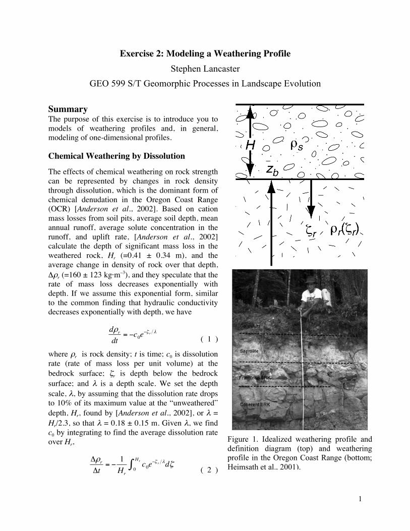
The effects of chemical weathering on rock strength can be represented by changes in rock density through dissolution, which is the dominant form of chemical denudation in the Oregon Coast Range (OCR) [Anderson et al., 2002]. Based on cation mass losses from soil pits, average soil depth, mean annual runoff, average solute concentration in the runoff, and uplift rate, [Anderson et al., 2002] calculate the depth of significant mass loss in the weathered rock, Hr (=0.41 ± 0.34 m), and the average change in density of rock over that depth, Δρr (=160 ± 123 kg·m–3), and they speculate that the rate of mass loss decreases exponentially with depth. If we assume this exponential form, similar to the common finding that hydraulic conductivity decreases exponentially with depth, we have

( 1 )

where ρr is rock density; t is time; c0 is dissolution rate (rate of mass loss per unit volume) at the bedrock surface; ζr is depth below the bedrock surface; and λ is a depth scale. We set the depth scale, λ, by assuming that the dissolution rate drops to 10% of its maximum value at the “unweathered” depth, Hr, found by [Anderson et al., 2002], or λ = Hr/2.3, so that λ = 0.18 ± 0.15 m. Given λ, we find c0 by integrating to find the average dissolution rate over Hr,

( 2 )

€

dρrdt

= −c0e−ζ r λ

€

ΔρrΔt

= −1Hr

c0e−ζ r λdζ

0

Hr∫

Figure 1. Idealized weathering profile and definition diagram (top) and weathering profile in the Oregon Coast Range (bottom; Heimsath et al., 2001).

2

setting the mass loss over the depth of significant weathering in the rock, ΔρrHr, equal to the mass loss in the soil, ΔρsH, (= 66.2 ± 19.4 kg·m–2, where H is soil depth) as in [Anderson et al., 2002], finding Δt from the depth, Hr, and the bedrock lowering rate, ε (= 0.1 ± 0.07 mm/a) [Anderson et al., 2002], to get

( 3 )

Solving for c0 and substituting values, the dissolution rate at the bedrock surface, c0 = 0.099 ± 0.096 kg·m–3·a–1.

Density-Dependent Physical Weathering

Physical weathering in the Oregon Coast Range is apparently dominated, at least in soil-mantled areas, by biotic action: rodent (Aplodontia rufa) burrowing and tree throw. My observations in the OCR (cf. [Lancaster et al., 2003]) indicate that sites denuded by landslides can remain bare of soil for decades, a period that is probably dependent on the probability of colluvium-trapping trees falling across the site and, therefore, on the age and size of the surrounding forest [May and Gresswell, 2003]. On sites of bare bedrock, it is likely that exfoliation due to unloading [Stock and Dietrich, 2006] and frost cracking [T.C. Hales and Roering, 2005; T. C. Hales and Roering, 2007] are most important for physical weathering. All of these processes involve overcoming the tensile strength of the rock and therefore likely depend on rock density [Stock and Dietrich, 2006], which is reduced by chemical weathering.

Rock density-dependent physical weathering is simulated by letting the bedrock-regolith conversion rate at zero colluvial depth vary with rock density:

( 4 )

where zb is the elevation of the bedrock surface; H is vertical colluvial depth; θ is the slope angle; hs is the slope-normal depth scale of the disintegration rate; εh is the minimum (hard-rock) zero-depth disintegration rate (e.g., 160 m/Ma; [Heimsath et al., 2001]); rrh is the density of unweathered rock (e.g., 2270 kg/m3 [115]); ew is the maximum (saprolite) zero-depth production rate (e.g., 350 m/Ma, the maximum value suggested by [Heimsath et al., 2001]); and rrw is the density of saprolite (e.g., 1150 kg/m3, the minimum density measured by [Anderson et al., 2002]). The term in brackets is the zero-depth disintegration rate, which is simply a linear function interpolating between eh and ew. The cosine term in the exponential is needed to relate vertical soil depth, H, to the slope-normal depth scale, hs.

This unwieldy expression with five parameters can be reduced to a simpler form with three parameters:

( 5 )

where

€

ΔρsH =λHrc0ε

1− e−Hr λ( )

€

dzbdt

= − εh +ρrh − ρrρrh − ρrw

⎛

⎝ ⎜

⎞

⎠ ⎟ εw −εh( )

⎡

⎣ ⎢

⎤

⎦ ⎥ e−H cosθ hs

€

dzbdt

= − ε0 −ερρr( )e−H cosθ hs

3

( 6 )

and

( 7 )

The density dependence in this model is obtained by essentially drawing a line between the maximum and minimum lowering rates measured by [Heimsath et al., 2001] at the minimum and maximum bedrock densities measured by [Anderson et al., 2002]. (What are some of the potential pitfalls of this sort of scheme?)

Finally, mass balance governs the thickness of the colluvium:

!"!"

= −!!!!!!!!"

+ ! + ! ( 8 )

where I and O are source (input) and sink (output) terms, e.g., to account for introduction of material from upslope and loss of material downslope.

New Tools

Before we get to the soil column model, we’ll cover some new Matlab tools, including type conversion, animation, matrix arithmetic, subplots, the “if statement,” and the “while loop.” You should now start up Matlab.

The While Loop: The model’s main loop is a “while loop,” which is similar to a for loop in the sense that the loop will continue to repeat as long as a specified condition is met. In the case of the for loop, the program incremented a “counter” variable (i.e., a variable that records the number of the current iteration of the loop) and tested its value against the total number of iterations desired. The while loop allows us to continue iterating through a loop as long as certain conditions are met, where we don’t already know how many iterations it will take to reach the desired end point. In this case, the while loop is

while z_br > z_br0-total_delz_br, …

end The “while” statement is followed by a so-called logical expression. Logical expressions have the value of one if true and zero if false. This loop will continue to iterate as long as the logical expression comparing the current bedrock elevation to the desired final bedrock elevation is true, i.e., as long as the current bedrock elevation is greater than the desired end point.

€

ε0 =εwρrh −εhρrwρrh − ρrw

€

ερ =εw −εhρrh − ρrw

4

The If Statement: The “if” statement is, like the “while” statement, followed by a logical expression, and like the while loop, the lines between “if” and “end” are executed only if the logical expression is true. The difference is that, with the if statement, those in-between lines are only executed once. Unlike the while loop, if statements can also contain alternatives, that is,

if a == b, % do something else if a == c, % do something else else % do a different thing end The “else if” statement allows specification of alternative conditions, and the “else” statement allows the programmer to make the model do something when none of the specified conditions are met.

Animation: Animation in Matlab is done by storing the contents of the current figure as a frame in an array of frames with the “getframe” command, changing those contents, storing another frame, and so on. The whole array of frames is then played with the “movie” command:

for i = 1:N … M(i) = getframe; end movie(M)

Matrix Arithmetic: In the last exercise, we assigned different values to members of an array by using a for loop:

Xdata = (0:2*pi/10:2*pi); for j=1:3 for i=1:11 Zdata(i,j) = cos(Xdata(i) - 0.5*(j-1)); end end It turns out we could have also done the same thing with the following:

Xdata = (0:2*pi/10:2*pi); for j=1:3 Zdata(:,j) = cos(Xdata - 0.5*(j-1)); end Instead of stepping through the rows of Zdata, we instead assign values to each of the three columns all at once. What a time saver! If we were really clever, we probably could have figured

5

out a way to forego the j-loop as well.

Type Conversion: Most of the time, we can perform arithmetic and not worry about whether we’re dealing with integers, real, or even complex numbers—Matlab is a lot less fussy about such things than most other programming languages. Sometimes, however, we need to specify that the result of some arithmetic must be an integer, or we wish to represent a number as a “string,” or text, to name the two most common cases.

By default, Matlab will store the results of arithmetic as type “double,” i.e., double-precision real numbers (single-precision real numbers are take up 32 bits or 64 bits in memory depending on whether you have a 32-bit or 64-bit processor; double-precision real numbers take up 64 bits or 128 bits, respectively). If, however, we want to use the result of the arithmetic as the index or size of an array, we need to make sure the number is stored as an integer. Type the following lines:

pi/3 int16(pi/3)

The first should have printed out “1.0472” and the second “1.”

When we want to use the value of a variable in, say, a title or label, we must convert the variable to a “string,” which is the computer-ese term for a series of text characters. Type the following:

int2str(int16(pi/3))

This will also print out “1” but without the preceding white space, an indication that Matlab now realizes that we have now asked it to be even more literal than it would be otherwise.

Subplots: Sometimes we want to include several graphs within the same figure window, for example, when several graphs share the same horizontal axis. In Matlab, this is done with the “subplot” command. Type the following lines:

figure subplot(3,1,1)

These commands will open a figure window and make a set of unit axes occupying only the top third of the figure. In the “subplot” command, the first number in parentheses specifies the number of rows of subplots, the second number specifies the number of columns, and the third number specifies which of the subplots we want to make “current” (i.e., subsequent “plot” and “label” commands will be applied to this subplot). The last number counts across and then down, i.e., if we typed

subplot(3,2,4)

6

it would indicate that we want to have six subplots in three rows and two columns and that we want the first subplot on the second row to be current.

Numerical Weathering Profile Model

Now, create a new M-file and name it something like “soil_column.m.” We’ll deal with the different parts of the model in turn.

First enter the lines to initialize the model’s constant parameters, some of which were discussed above:

% initialize process parameters: l_depth_decay=0.18; % depth scale for chem. weath., m Hs_depth_decay=0.30; % depth scale for phys. weath., m rho_rh=2270; %initial unweathered bedrock bulk density, kg/m3 rho_rw=1150; %saprolite (weathered rock) bulk density, kg/m3 rho_s=740; %soil bulk density, kg/m3 (Anderson et al., 2002) eps_h=1.6e-4; %minimum hard-rock zero-depth phys. weath. rate, m/yr eps_w=3.5e-4; %maximum saprolite phys. weath. rate, m/yr C_0=0.099; %dissolution rate at bedrock surface, kg/m3/yr % initialize numerical parameters: dt=1.0; %time step, yr nT=500; %number of time steps between plotting Tviz=0.0; %time for making next plot, yr N_layers_per_lambda=20; %number of layers in bedrock delta_zeta=l_depth_decay/N_layers_per_lambda; %discretization of bedrock, m zeta_bottom=2.0; %maximum depth in calculations, eff. unweathered depth, m total_delz_br=1.2; %total bedrock lowering during simulation, m z_br0=100.0; %initial bedrock elevation, m H_init=0.0; %initial soil depth, m H_next=1.0; % initialize soil source term: extra_dH_dt=0; %rate of accumulation from upslope, m/yr While the initial soil depth is here set to zero, one could forego “spin-up” time by setting the initial depth, H_init, to the final steady-state soil depth, H_next.

Next, the following lines initialize the model’s variables:

% initialize spatial variables: zeta=delta_zeta:delta_zeta:zeta_bottom; %depth below bedrock surface, m num_del_zeta=int16(zeta_bottom/delta_zeta); %number of bins in rock column rho_r=zeros(1,num_del_zeta)+rho_rh; % hard-rock bedrock density, kg/m3 z_br=z_br0; %bedrock surface elevation, m H=H_init; %soil depth, m % initialize time series variables to zero b/c we don't know the right size H_series=0.0; rho_r1_series=0.0; z_br_series=0.0; time_series=0.0; clear F

7

% initialize "counter" variables: i=1; m=0; run_time=0.0; % set initial values of time series: H_series(i)=H; rho_r1_series(i)=rho_r(1); z_br_series(i)=z_br; time_series(i)=run_time; Note that we used three of our new tools: (1) we used the “int16” command to convert the ratio, zeta_bottom/delta_zeta, into a number that could be used as one of the dimensions of a new array, and (2) we used matrix addition with the “zeros” command to initialize the whole rho_r array to the same value. We could have gotten the same result by using the “ones” command (which makes an array in which all values are equal to one) and multiplication.

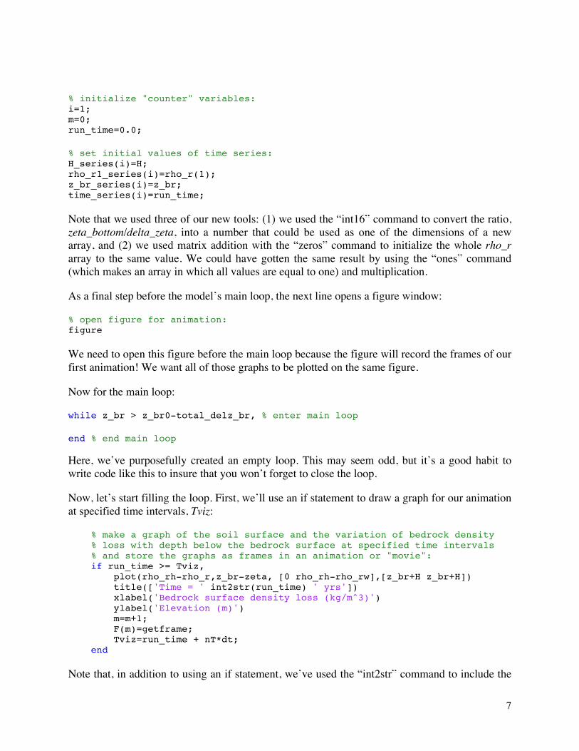
As a final step before the model’s main loop, the next line opens a figure window:

% open figure for animation: figure We need to open this figure before the main loop because the figure will record the frames of our first animation! We want all of those graphs to be plotted on the same figure.

Now for the main loop:

while z_br > z_br0-total_delz_br, % enter main loop end % end main loop Here, we’ve purposefully created an empty loop. This may seem odd, but it’s a good habit to write code like this to insure that you won’t forget to close the loop.

Now, let’s start filling the loop. First, we’ll use an if statement to draw a graph for our animation at specified time intervals, Tviz:

% make a graph of the soil surface and the variation of bedrock density % loss with depth below the bedrock surface at specified time intervals % and store the graphs as frames in an animation or "movie": if run_time >= Tviz, plot(rho_rh-rho_r,z_br-zeta, [0 rho_rh-rho_rw],[z_br+H z_br+H]) title(['Time = ' int2str(run_time) ' yrs']) xlabel('Bedrock surface density loss (kg/m^3)') ylabel('Elevation (m)') m=m+1; F(m)=getframe; Tviz=run_time + nT*dt; end Note that, in addition to using an if statement, we’ve used the “int2str” command to include the

8

value of the run_time variable in the title so that the frames of our animation will be time-stamped.

The following lines contain the “guts” of the model by describing the change in density due to chemical weathering, the changes in bedrock surface elevation and soil thickness due to physical weathering (and, for soil thickness, the upslope source):

del_rho = -C_0 * exp(-zeta / l_depth_decay) * dt; delz_br = -(eps_h + ((rho_rh-rho_r(1)) / (rho_rh-rho_rw)) ... * (eps_w-eps_h)) * exp(-H / Hs_depth_decay) * dt; delH = -rho_r(1)/rho_s * delz_br + extra_dH_dt * dt; z_br = z_br + delz_br; rho_r = rho_r + del_rho; H = H + delH; Note that we’ve made extensive use of matrix arithmetic, but we’ve been careful to use only one array in each line of matrix arithmetic, e.g., when we add a scalar to a vector, that scalar value is added to each term of the vector. Next, we need to address the bookkeeping of our bedrock layers. By lowering the bedrock surface elevation, we’ve reduced the depth of all of our bedrock layers by the amount of that lowering:

zeta = zeta + delz_br; Now, we want to be sure that, if we’ve removed all of the rock from one of the layers, we eliminate that layer and that we don’t eventually exhaust our initial supply of layers:

if zeta(1) <= 0.0, zeta = zeta + delta_zeta; rho_temp=rho_r; rho_r(1:num_del_zeta-1)=rho_temp(2:num_del_zeta); rho_r(num_del_zeta)=rho_rh; end Our if statement says that if the depth of the first layer is zero or negative, then we increase the depth of all layers by one layer thickness (delta_zeta), make the second layer first, and add a new layer of unweathered bedrock at the bottom.

The next lines serve to cap the soil thickness at a constant value:

if H > H_next, H=H_next; end In one of your exercises, you will need to figure out how to make the soil be stripped when reaching a threshold value. The previous if statement is where you will do that.

Finally, we increment the run time and the index for our time series and record variable values in those time series:

run_time=run_time+dt; i=i+1; H_series(i)=H;

9

rho_r1_series(i)=rho_r(1); z_br_series(i)=z_br; time_series(i)=run_time;

Note that every time we add another value to the series, we are changing their lengths. This is computationally costly because Matlab must copy the arrays into new, larger arrays every time we do this. This cost is the reason that, when we can, we use the “zeros” or “ones” command to initialize our arrays to their full sizes. In the above case, we didn’t know beforehand how many iterations it would take to lower the bedrock surface by the desired amount, so we didn’t know how big the arrays would need to be. Note that the next line should now be the “end” of the main loop.

After the loop is done, we want to look at the results:

movie(F,2,2) figure subplot(3,1,1), plot(time_series,H_series), ylabel('soil depth (m)') subplot(3,1,2), plot(time_series,rho_r1_series), ... ylabel('density loss (kg/m^{-3})') subplot(3,1,3), plot(time_series,z_br_series), ... ylabel('bedrock surface elevation (m)'), xlabel('time (yr)') The first line plays the movie back twice at 2 frames per second. (Note: In my tests, the timestamp is not updated during the movie playback. Hmph.) The next lines use the subplot command to make a column of three graphs of the time series.

An Alternative Model of Physical Weathering by Frost Cracking

As shown in class, fluctuations in temperature at the surface and the diffusion of those fluctuations with depth beneath the surface generally lead to a maximum in frost cracking at a finite depth beneath the surface. For annual and daily fluctuations in surface temperature, we may represent temperature, T, as a function of time and depth as follows:

! = !! + !!!!!! !∗!!"#2!"!!

−!!!∗!

+ !!!!!! !∗!!"#2!"!!

−!!!∗!

( 9 )

where T0 is mean annual temperature; Ta and Td are the amplitudes of the annual and daily temperature fluctuations; ζs is the depth below the surface; ζ∗s and ζ∗d are the depth scales for penetration of annual and daily fluctuations, respectively; Pa and Pd are the annual and daily periods (i.e., 365 days and 1 day), respectively; and t is time. We can use this equation to determine the time spent in the temperature range in which frost cracking is active, i.e., the frost cracking window, typically –8 to –3 °C. If I were more clever, maybe I could figure out how to find an analytical solution for the time spent in the frost cracking window. Since I’m not so clever, I’ll do it numerically.

Open another new M-file, name it something like “frost_cracking_window.m,” and enter the following code. First are the initializations:

10

% initialize constants: Ta=15; Td=15; T0=5; zsa=3; zsd=0.2; Pa=365; Pd=1; % initialize independent variables: t=0:0.01:365; z=0:0.01:5; % initialize dependent variables: T=zeros(length(z),length(t)); STc=zeros(size(z)); Then come the calculations:

% calculate temperatures: for i=1:length(t), T(:,i)=T0+Ta*exp(-z/zsa).*sin(2*pi*t(i)/Pa-z/zsa)+... Td*exp(-z/zsd).*sin(2*pi*t(i)/Pd-z/zsd); end % calculate time in frost cracking window: for j=1:length(z), I=find(T(j,:)>=-8 & T(j,:)<=-3); STc(j)=length(I)*0.01/Pa; end You might notice something different about the matrix arithmetic in the temperature calculation: the multiplication symbols between the exponential and sine terms are preceded by periods, (i.e., “.*”). This syntax indicates term-by-term multiplication of the terms of the two arrays rather than true matrix multiplication.

Finally, graph the results:

plot(STc,-z) The resulting function, STc, can be used to determine the dependence of physical weathering rate on soil depth (i.e., we won’t try to apply physical weathering within the bedrock column but, rather, only on the surface layer, as with the physical weathering function previously described and implemented). Note that you can call one script within another.

Exercises

1. Use the weathering model (soil_column.m) to predict a relationship between steady-state bedrock lowering rate and soil depth. Note that it takes some time after the soil depth reaches its equilibrium value before the bedrock density profile reaches it equilibrium shape and, therefore, the soil production rate reaches its equilibrium value.

2. Edit the code to produce cycles of soil depth increase between episodes of stripping once a threshold depth is surpassed. Use variations in the soil source term, extra_dH_dt, to vary the period of these cycles and use the model to predict a relationship between that period and steady-state bedrock lowering rate.

3. Use the frost-cracking model (frost_cracking_window.m) to replace the exponential dependence on soil depth in the physical weathering function with a numerically

11

calculated soil depth dependence (i.e., keep everything, particularly the dependence on bedrock density, except for the exponential term). Use the revised model to predict the relationship between bedrock lowering rate and soil depth and between bedrock lowering rate and mean annual temperature, T0. How would bedrock lowering rate vary over a long slope with significant and systematic variations in mean annual temperature (decreasing temperature with increasing elevation) and soil depth (e.g., decreasing soil depth with increasing elevation)?

Submit your M-files that reflect changes prescribed above to me as attachments in an email before the time/date at which the assignment is due. Make certain that your M-files “run” to your satisfaction without errors before submitting them. Make sure your email has the subject line, “GEO 599 Exercise 2: <lastname>,” where you should substitute your own last name for the bit in angle brackets. Also submit a written report (as an email attachment) explaining the prescribed examinations with the models. Embed figures in your report by saving them as EPS files from Matlab and dragging or importing them into your document. The report can be as brief as you can make it, but it should explain exactly what you did (methods) and what your results are. Don’t try to produce a manuscript with introduction, discussion, and conclusions.

References

Anderson, S. P., W. E. Dietrich, and G. H. Brimhall (2002), Weathering profiles, mass-balance analysis, and rates of solute loss: Linkages between weathering and erosion in a small, steep catchment, GSAMB, 114(9), 1143-1158.

Hales, T. C., and J. J. Roering (2005), Climate-controlled variations in scree production, Southern Alps, New Zealand, Geo, 33(9), 701-704.

Hales, T. C., and J. J. Roering (2007), Climatic controls on frost cracking and implications for the evolution of bedrock landscapes, J. Geophys. Res., 112.

Heimsath, A. M., W. E. Dietrich, K. Nishiizumi, and R. C. Finkel (2001), Stochastic processes of soil production and transport: Erosion rates, topographic variation and cosmogenic nuclides in the Oregon Coast Range, ESPL, 26(5), 531-552.

Lancaster, S. T., S. K. Hayes, and G. E. Grant (2003), Effects of wood on debris flow runout in small mountain watersheds, WRR, 39(6), 1168.

May, C. L., and R. E. Gresswell (2003), Processes and rates of sediment and wood accumulation in headwater streams of the Oregon Coast Range, USA, ESPL, 28(4), 409-424.

Stock, J. D., and W. E. Dietrich (2006), Erosion of steepland valleys by debris flows, GSAMB, 118, 1125-1148.