Chemical Data Assimilation Experiment of Real Data based ... · the chemical data assimilation are to be ”forgotten” due to diffusion process. Meanwhile the emis-sion rates and

www.dmi.dk/dmi/sr14-03.pdf page 1 of 19

Scientific Report 14-03

Chemical Data Assimilation Experiment of Real Data based on Online Integrated Enviro-HIRLAM Model Output

Alexey Penenko1,2, Vladimir Penenko1, Roman Nuterman3,4,5, Alexander Baklanov3,6, Alexander Mahura3

1 Institute of Computational Mathematics and Mathematical Geophysics SB RAS, ICM&MG SB RAS, prospekt Akade-mika Lavrentjeva 6, 630090, Novosibirsk, Russia

2 Novosibirsk State University, NSU, Pirogova Str. 2, 630090, Novosibirsk, Russia 3 Danish Meteorological Institute, DMI, Lyngbyvej 100, DK-2100, Copenhagen, Denmark 4 University of Copenhagen, Nørregade 10, PO Box 2177, 1017 Copenhagen K, Denmark

5 Tomsk State University, TSU, Lenin Ave., 36, 634050, Tomsk, Russia 6 World Meteorological Organization, WMO, 7bis av. la Paix, CP2300, CH-1211, Geneva, Switzerland

Copenhagen 2014



Colophon Serial title: Scientific Report 14-03 Title: Chemical data assimilation experiment of real data based on online integrated Enviro-HIRLAM model output Subtitle: --- Author(s): Alexey Penenko, Vladimir Penenko, Roman Nuterman, Alexander Baklanov, Alexander Mahura Other contributors: --- Responsible institution: Danish Meteorological Institute Language: English Keywords: Discrete-Analytical schemes, splitting method, fine-grained data assimilation, chemical data assimi-lation, variational approach, convection-diffusion-reaction model Url: www.dmi.dk/dmi/sr14-03.pdf Digital ISBN: 978-87-7478-657-3 (on-line) ISSN: 1399-1949 (on-line) Version: - Website: www.dmi.dk Copyright: Danish Meteorological Institute Application and publication of data and text is allowed with proper reference and acknowledgement



Content: Abstract ................................................................................................................................................ 4 1. Introduction .................................................................................................................................. 4 2. Data Assimilation Algorithm ....................................................................................................... 5

2.1. Transport and Transformation Model ....................................................................................... 5 2.2. Fine-Grained Data Assimilation to the Model .......................................................................... 7

3. Input Data Analysis .................................................................................................................... 10 4. Chemical Data Assimilation ...................................................................................................... 12

5.1. Data Assimilation Scenario ..................................................................................................... 12 5.2. Data Assimilation Results ....................................................................................................... 13

5.2.1. Site-wise division ............................................................................................................. 13 5.2.2. Temporal difference ......................................................................................................... 17 5.2.3. Species exclusion experiment .......................................................................................... 18

Conclusion ......................................................................................................................................... 18 Acknowledgements ............................................................................................................................ 19 References .......................................................................................................................................... 19



Abstract

Results of numerical experiments with chemical data assimilation algorithm of in situ concentration measurements on real data scenario have been presented. The algorithm is based on the variational approach and splitting scheme. This allows avoiding iterative direct problems solution for transport and transformation model and the algorithm becomes a “real-time algorithm”. In order to construct test scenario, meteorological data has been taken from Enviro-HIRLAM output, initial conditions from MOZART model output and measurements from Airbase database.

1. Introduction We consider the following classes of problems associated to the inverse modeling:

Direct problems: System’s behavior has to be forecasted and studied with a mathe-matical model. Inverse problems: Model parameters must be adjusted to fit model forecasts to the corresponding measurement data. It may take to solve series of direct problems with various model parameters. Data assimilation problems: A forecast has to be improved (on-line) by adjusting model parameters with incoming measurement data. It may take to solve series of inverse problems with various measurement data.

In this work we present data assimilation algorithm for convection-diffusion part of atmospheric chemistry model. To construct a data assimilation algorithm, the following properties should be taken into account:

Atmospheric composition is being changed rapidly, therefore current and future sys-tem state is of interest. Chemical weather forecast in ”Real-time”. Stiff chemical kinetics equations (different time scales), various chemical mechanisms and their nonlinear behavior. Uncertainties are not only in initial conditions but also in model coefficients (reaction rates) and in emission rates. High dimensionality ( ) of modern atmospheric chemistry transport models due to high number of spatial variables and different species, imposes requirements to the com-putational performance. Relatively small number of chemical species in a small number of spatial points can be measured. Data assimilation algorithms must be embedded in existing models. Multi-disciplinary study.

A review and examples of chemical data assimilation algorithms can be found in [1, 2, 3]. Summa-rizing them, we would like to emphasize that unlike data assimilation in meteorology initial states in the chemical data assimilation are to be ”forgotten” due to diffusion process. Meanwhile the emis-sion rates and model coefficients play a significant role as the sources of uncertainty in the chemical data assimilation. In our work we use source-term uncertainty to perform data assimilation. The report is a continuation of [4]. The current work has the following purposes:

To compile a complete realistic scenario to evaluate data assimilation algorithms pre-sented in the previous report [4]. In order to apply a Data Assimilation algorithm to real data, one has to prepare a con-sistent set of parameters:

Meteorological conditions for transport and transformation of model parameters. Chemical background for initial and boundary conditions.



Measurement data have to be reduced to a common form and divided into assimi-lated and reference sets.

The data assimilation algorithm has to be applied to the assimilated set and compared to a reference one.

2. Data Assimilation Algorithm

2.1. Transport and Transformation Model Let us consider a spatial-temporal domain:

, , ∈ Ω 0, 0, 0, , ∈ 0, , Ω : Ω 0, .

bounded by Ω Ω 0, . In the domain we consider atmospheric chemistry transport and transformation model for different substances like contaminants, heat, moisture, radiation, etc.

≡,

div , , grad ,

, , , , , ∈ Ω , (1)

,,

, , , , , ∈ Ω , (2)

, 0 , ∈ Ω. (3)

Here , is a state function that has physical meaning of concentrations fields at point , ∈Ω , e.g. , corresponds to the concentration of substance at point , . Here 1, . . . , ,

is the number of considered substances. Vector , , , , , , de-notes ”wind speed”, , , , , , , is a diagonal diffusion tensor, : → is a transformation operator, is the boundary outer normal direction, , , , , - a priori data for the sources and initial data, , is a control function (uncertain-

ty), that is introduced in the perfect model structure to assimilate data. As it is for , , each entry of , , , , , , vectors corresponds to a quantity attributed to l-th substance at point , . Transformation operator is defined by the chemical kinetics system of 22 reacting species from [5, 6] augmented with the reaction taken from the CMAQ model [7]:

hv NO2 → NO O3P hv O3 → O1D O2HCHO hv → CO 2. HO2 HCHO hv → CO H2

O2 O3P → O3 N2 O1D → N2 O3PO1D O2 → O2 O3P H2O O1D → 2. OHHO2 NO → NO2 OH NO O3 → NO2 O2

NO RO2 → HCHO HO2 NO2 CO OH → CO2 HO2HC OH → H2O RO2 HCHO OH → CO H2O HO2NO2 OH → HNO3 2. HO2 → H2O2 O2

H2O 2. HO2 → H2O H2O2 O2 HO2 RO2 → O2 ROOH2. RO2 → Prod OH SO2 → HO2 Sulf

Reaction rates have been taken from [5] and depend on time, i.e, photochemistry is considered.

This kinetics system can be presented in the production-destruction operator form: , , , Π , , 1, . . . , , (4) , Π : → . (5)



Direct problem: With given , , , determine from (1)-(3). Exact solution ∗ is a solution of direct problem corresponding to ”unknown” emissions ∗. We consider all the functions and model parameters to be smooth enough for the solutions to exist and further transformations to make sense.

For the numerical solution let us introduce uniform temporal grid on 0, with step

size and points and uniform spatial grids with , 1,2,3 grid points on Ω, . Let be the space of real grid functions on . Direct problem can be efficiently

solved with splitting method. Let us consider additive-averaged splitting scheme (analogous to [8]) on the intervals . The splitting is done with respect to physical process (advection-diffusion and transformation processes) and advection-diffusion part is further split with respect to spatial dimensions. Finally we have 4 parallel stages for the step partition ∑ 1 and sources

partition ∑ .

Convection-diffusion processes ( 1,2,3) ,

, , , ,

, , , , ∈ Ω , ,

,,

, , , , , ∈ Ω , ,

, , , ∈ Ω, where Ω ∈ Ω| 0|| . This initial value problem can be approximated with implicit matrix form:

, (6)

: . (7)

Here ∈ stands for the solution on the -th time layer, ∈ is the uncer-tainty on the j-th time layer and : → are approximated advection-diffusion operators from (1) corresponding to spatial dimensions. Chemical reaction processes ( 4)

,, ,

Π , , , , , ∈ Ω , ,

, , , ∈ Ω, or in the entry-wise form

,, ,

Π , , , , , ∈ Ω , , 1, . . . , .

where is the destruction rate functional and Π is the production functional. In [9,10,11] a family of unconditionally monotonic schemes have been built, from the first to fourth order of accuracy. One of the single stage schemes is equivalent to the known QSSR scheme [12]:

, 1, . . . , , ∈ ,



1

Π ,

1

.

In vector form . (8)

Next step approximation

. (9)

Advantage of the scheme is that individual processes for each dimension are evaluated independent-ly (in parallel).

2.2. Fine-Grained Data Assimilation to the Model In order to assimilate measurement data, we have to connect measured quantities with the model variables. This is formally done with the measurement operator : , ∗ . , , ∈ 0, , (10)

where are measurement data, ∗ . , is ”true” (or exact) solution, is measurement data uncertainty. Data assimilation problem: Determine . , for ∗ with (1)-(3), (10) and functions , , , defined on 0 ∗.

In the work we consider in situ measurements at the domain grid points , ⊂

. Hence the m-th measurement is defined by the vector , , , , , 1, . . . , .

where is the spatial coordinate of the measurement, is the moment of measurement, is the number of substance measured, is the resulting concentration and is the standard variation of the measurement. According to the data assimilation problem statement in a time-step we can use only measurements with . Let us define the set of indices

1 | . The corresponding measurement operator

,∈

,

∈ , ∈ . A function is from a set of admissible values that describe error estimate for measurement data. The error is considered to be bounded in (weighted) Euclidean norm in the measurements space

‖ ‖∈

.

Variational data assimilation provides the solution to a data assimilation problem as the minimum of the functional with the constraints imposed by the model. The functional usually combines measurement data misfit with a norm of a control variable:



, ‖ ‖ , where ‖. ‖ is the norm of a Hilbert space over and . , . is the corresponding inner product,

is the regularization (assimilation parameter), which selects whether the solution will be closer to the direct model solution or will reproduce measurements better. In the paper on the time step we update only the control variable for this time step. In the context of assimilating data to the split model we distinguish between the two approaches:

In conventional approach [13, 14] one takes minimum of , as the solution with constraints (6), (8), (9) and , i.e., control functions of different splitting stages are connected. In the fine-grained approach [15, 16, 17] the same data are assimilated to different parts of model and the results are coupled afterwards. We seek for the minimum of the func-tional

, ,

on constraints (6), (8) with the independent .

Using the method of Lagrange multipliers to solve minimization problem with equality con-straints, we can construct augmented functional:

, , ,

,

We can see that components of , corresponding to different are independent hence

stationary point coordinates can be found independently. In order to present an algorithm of finding a stable point for the convection-diffusion

part, we need further elaboration of operator . As a result of splitting we can consider equations (6) independent for each coordinate line in both dimensions. The algorithm is the same for any coordi-nate line and here we will describe the algorithm applied the -th grid line along X axis for a given 1 and l-th substance field. Let , , , 1

: . For the sake of computational efficiency we use approximations of (1) that produce tridiagonal matrix systems:

, 0, (11)

, 1, … , 1, (12)

, . (13) In this term the assimilated state is the solution of the minimization problem

, ,



WRT (11)-(13) where is the spatial-temporal measurement mask (i.e. equals 1 if ∈

and 0 otherwise, in other words, it is equal to 1 if there is a measurement data at point ), is measurement data at point (if there is a measurement) and is measurement device standard deviation of the measurement in point (if there is a measurement). Introducing Lagrange multi-pliers, we obtain augmented functional:

, , ∗ , ∗ .

Taking the first variations of the augmented functional equal to zero, we obtain the following equations:

∗ , , ∗ 0, which is equivalent to (11)-(13).

, , ∗ 0

is equivalent to

2, 0,

2, 1, … , 1,

2, .

and

, , 0

is equivalent to 2 0, 0, … , .

The systems obtained can be merged into tridiagonal matrix equation [15,16,17]

Φ Φ , 0, Φ Φ Φ , 1, . . . , 2,

Φ Φ , 1,

00 ,

22 ,

00 ,

Φ , 2 ,

which is solved by the direct matrix sweep method. For the transformation step data assimilation the algorithm is the same for any grid

point ∈ . For brevity let ∈ , ∈ , ∈ and the



result is sought as the stationary point of the augmented functional

,

1Π .

where is equal to 1 if l-th substance is measured at point at moment and zero otherwise. This minimum is given by the formula:

11

1Π

1,

1.

As we can see, the resulting algorithm can be implemented without iterations.

3. Input Data Analysis

In our model we use ppb as basic concentration units. To compile the scenario to test Data Assimi-lation, we have used the following datasets:

Airbase - European atmospheric composition measurement data [18]. We have used data from 22 Scandinavian (DK, SE, FI, NO) measurement sites. There are 64001 in total

, , , , measurements for the considered period of time. Concentration data for substances , , , is given in ug/m3 and for in mg/m3. Conversion formula

8314⋅⋅

,

where Concentration is concentration in [ppb], is concentration [ug/m3], is temperature [K], is molecular weight in [ams], is pressure in [Pa]. And

1000 ∗ 8314⋅⋅

,

where is concentration [mg/m3]. MOZART IFS data is used as initial conditions. Dataset contains , , , ,

, , , concentration fields in [mole/mole] Conversion formula [19]: ∗ 10 .

where Concentration is concentration in [ppb], vmr is volume mixture ratio in [mole/mole]. Enviro-HIRLAM output has been used for meteorological data [20].

In order to check data consistency, we have conducted some basic correlation study. We’ve chosen since its concentrations were present in both datasets from MOZART and Enviro-HIRLAM. In

figures 1 and 2 we can see that models performance can vary. In this case Enviro-HIRLAM did better estimate (r = 0.31) than MOZART (r = -0.1) for measurement site DK0021A. Time series are presented to the left and scatter plots to the right.



Figure 1. Time series comparison at the measurement site (left). Scatter plot of measurements vs

MOZART-IFS model output (right).

Figure 2. Time series comparison at a measurement site (left). Scatter plot of measurements vs Enviro-

HIRLAM model output (right).

Figure 3. Time series comparison at a measurement site (left). Scatter plot of measurements vs Enviro-

HIRLAM model output (right).

The second numerical experiment was devoted to estimation of the correlation with respect to time of a day. In figures 4 and 5 we can see that the correlation is better for the day-time (from 5 am to 8 pm) and slightly drops in the night-time.



Figure 4. Measurements vs Enviro-HIRLAM model output correlation with respect to time of day (for July

2010).

Figure 5. Measurements vs Enviro-HIRLAM model output correlation with respect to time of day (for July

2010).

4. Chemical Data Assimilation

5.1. Data Assimilation Scenario In our numerical experiments we have done the following simplifications with respect to the data assimilation problem statement:

The model used is a 2D model; Zero Neumann boundary conditions are used (to be taken from MOZART); Simple transformation mechanism (22 chemical reactions); Transformation rates depend only on time of a day (important to account for pressure and

temperature), revised parameters will be useful; Available emission databases are needed (annual update is desirable for operational use); A simplified diffusion coefficient is used.

In the data assimilation, we have used, the domain which is defined by temporal and spatial grids:

Temporal grids: - Physical time span: 1 July 2010 - 1 August 2010. - Temporal grid for transport processes

3720 ∗ 720 31 . - Nested temporal grid for transformation processes is 100 times finer:



372000 ∗ 7.2 31 . Spatial grids: (5 times coarser than Enviro-HIRLAM grid in each dimension):

61 ∗ 83 5086 , 61 ∗ 81 4962 .

Transport model parameters have been taken from the Enviro-HIRLAM meteorological output. We have used wind speed at 10m components (U10, V10). Diffusion coefficient is evaluated from the wind speeds. Measurement Data have been taken from AirBase - the European Air quality database [5]. We have used 64001 SO2, CO, NO, O3, NO2 measurements in total from 22 Scandinavian (DK - Denmark, SE - Sweden, FI - Finland, NO - Norway) measurement sites (Fig.6).

Figure 6. Computation domain and measurement sites locations (red dots).

To study impact of both transformation and data assimilation processes, we have considered four configurations encoded by:

DATrspT(rns): Transformations with data assimilation to transport processes; TrspTrns: Transformations with transport processes without data assimilation; DATrsp: Data assimilation to transport processes without transformation; Trsp: Transport processes (with neither transformation nor data assimilation).

5.2. Data Assimilation Results To compare configurations, some part of measurements are assimilated the rest is used as reference. The choice of division criteria defines a numerical experiment. Results are compared with respect to correlation coefficient and RMSE.

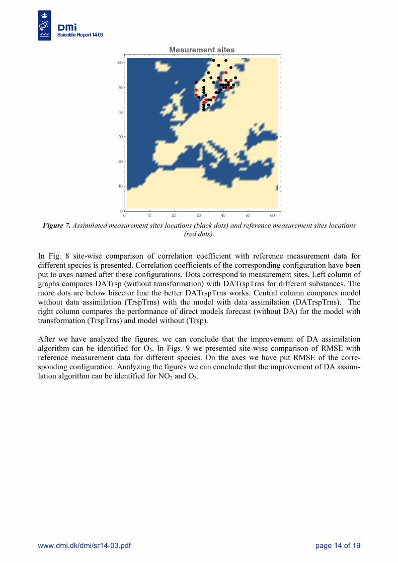
5.2.1. Site-wise division In this experiment we assimilated 80% of data on sites and used the rest of data for reference (Fig.7).



Figure 7. Assimilated measurement sites locations (black dots) and reference measurement sites locations

(red dots).

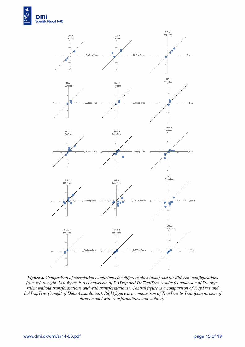
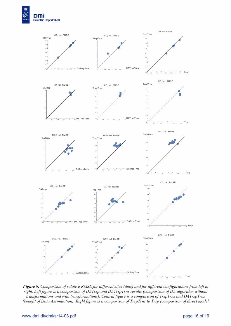
In Fig. 8 site-wise comparison of correlation coefficient with reference measurement data for different species is presented. Correlation coefficients of the corresponding configuration have been put to axes named after these configurations. Dots correspond to measurement sites. Left column of graphs compares DATrsp (without transformation) with DATrspTrns for different substances. The more dots are below bisector line the better DATrspTrns works. Central column compares model without data assimilation (TrspTrns) with the model with data assimilation (DATrspTrns). The right column compares the performance of direct models forecast (without DA) for the model with transformation (TrspTrns) and model without (Trsp). After we have analyzed the figures, we can conclude that the improvement of DA assimilation algorithm can be identified for O3. In Figs. 9 we presented site-wise comparison of RMSE with reference measurement data for different species. On the axes we have put RMSE of the corre-sponding configuration. Analyzing the figures we can conclude that the improvement of DA assimi-lation algorithm can be identified for NO2 and O3.



Figure 8. Comparison of correlation coefficients for different sites (dots) and for different configurations from left to right. Left figure is a comparison of DATrsp and DATrspTrns results (comparison of DA algo-rithm without transformations and with transformations). Central figure is a comparison of TrspTrns and

DATrspTrns (benefit of Data Assimilation). Right figure is a comparison of TrspTrns to Trsp (comparison of direct model win transformations and without).



Figure 9. Comparison of relative RMSE for different sites (dots) and for different configurations from left to right. Left figure is a comparison of DATrsp and DATrspTrns results (comparison of DA algorithm without

transformations and with transformations). Central figure is a comparison of TrspTrns and DATrspTrns (benefit of Data Assimilation). Right figure is a comparison of TrspTrns to Trsp (comparison of direct model



win transformations and without).

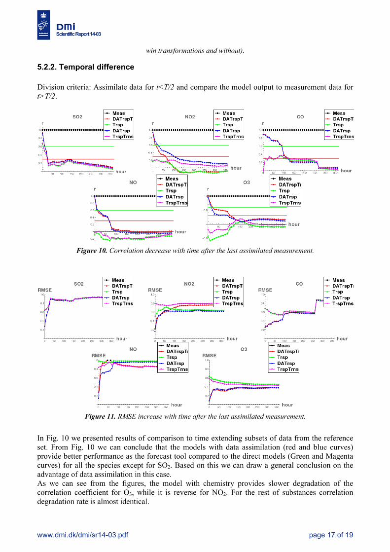
5.2.2. Temporal difference Division criteria: Assimilate data for t<T/2 and compare the model output to measurement data for t>T/2.

Figure 10. Correlation decrease with time after the last assimilated measurement.

Figure 11. RMSE increase with time after the last assimilated measurement.

In Fig. 10 we presented results of comparison to time extending subsets of data from the reference set. From Fig. 10 we can conclude that the models with data assimilation (red and blue curves) provide better performance as the forecast tool compared to the direct models (Green and Magenta curves) for all the species except for SO2. Based on this we can draw a general conclusion on the advantage of data assimilation in this case. As we can see from the figures, the model with chemistry provides slower degradation of the correlation coefficient for O3, while it is reverse for NO2. For the rest of substances correlation degradation rate is almost identical.



Looking at RMSE degradation in Fig. 11 we can confirm the conclusion of data assimilation bene-fits. Comparing DATrsp and DATrspT, we can state that RMSE degradation rate (its increase) for DATrspT for all species is higher than for DATrsp. Probably it is because of more uncertain and nonlinear nature of DATrspT with chemical transformations.

5.2.3. Species exclusion experiment Division criteria: Assimilate all the data except for data of the selected substance.

Species Meas DATrspTrns Trsp DATrsp TrspTrnsCO 1. 0.0420364 0.041718 0.041718 0.042036

NO 1. 0.370355 -0.068419 -0.068419 -0.035124

NO2 1. 0.458236 0.063321 0.063321 -0.019848 SO2 1. -0.014101 -0.016041 -0.016041 -0.014101

O3 1. 0.119529 -0.058031 -0.058031 -0.029600

Table 1. Comparison of results for different excluded species.

As we can see from Table 1, the best performance for DA with chemical transformations has been obtained for NO2 and NO. This can be explained by a strong link between the two species. In case the concentration of one of them is known, the other can be reconstructed. Less improvement has been obtained for O3 (below significant correlation level of 0.3). For CO and SO2 the results of all configurations have been almost the same.

Conclusion

Combination of splitting and data assimilation schemes let us construct computationally effective algorithms for data assimilation of in-situ measurements to convection-diffusion models. A complete data assimilation scenario has been compiled with meteorological data from Enviro-HIRLAM model, initial concentration data from the MOZART model and in-situ measurement data from AirBase. We carried out series of numerical experiments in which we tested data assimilation algorithms on different divisions of measurement data into assimilated and reference datasets. Data assimilation was able to improve modeling results with imperfect (approximate) models and model parameters. The advantage of data assimilation algorithm that includes chemical transformations was identified for ozone concentrations modeling. Among the future steps to improve data assimilation results we can identify:

Inclusion of more realistic boundary conditions is required; Additional tuning is essential for coefficients of chemical reactions; Quality control of chemical data measurements at stations is recommended for exclud-

ing ”extreme” data; Revision of implementation procedure/steps for chemical model is required; Additional evaluation of monthly and seasonal variability is needed.



Acknowledgements Authors are thankful to DMI colleagues for constructive comments and discussions. Authors appreciate Irina Gerasimova’s help with the text of report. The work has been partially supported by COST Action ES1004 (http://eumtechem.info) STSM Grant #21654, RFBR 14-01-31482 mol_a and 14-01-00125, Programs # 4 Presidium Russian Academy of Science (RAS) and # 3 MSD RAS, integration projects Siberian Branch RAS #8 and #35.

References [1] A. Sandu and C. Tianfeng. Chemical data assimilation - an overview. Atmosphere, 2:426–463, 2011. [2] Baklanov A. et. al. Online coupled regional meteorology chemistry models in Europe: current status and

prospects. Atmos. Chem. Phys., 14:317–398, 2014. [3] Elbern H.,Strunk A., Schmidt H., Talagrand O., Emission rate and chemical state estimation by 4-

dimensional variational inversion. Atmos. Chem. Phys. 2007. Vol.7. P.3749-3769. [4] Penenko, A., Penenko, V., Nuterman, R., Mahura, A. Discrete-Analytical Algorithms for Atmospheric

Transport and Chemistry Simulation and Chemical Data Assimilation. DMI Scientific Report 14-02 (2014) www.dmi.dk/dmi/sr14-02.pdf

[5] William R. Stockwell and Wendy S. Goliff Comment on “Simulation of a reacting pollutant puff using an adaptive grid algorithm” by R. K. Srivastava et al. JOURNAL OF GEOPHYSICAL RESEARCH, 2002 V 107 No D22.

[6] Gery, M.W. G.Z. Whitten, J.P. Killus, and M.C. Dodge, A photochemical kinetics mechanism for urban and regional scale computer modeling, J. Geophys. Res., 94, 12, 952-12,956,1989

[7] Byun, D. W. and Schere, K. L.: Review of the governing equations, computational algorithms and other components of the Models-3 Community Multiscale Air Quality (CMAQ) Modeling System, Applied Mechanics Reviews, 59(2), 51–77, 2006.

[8] A.A. Samarskii and P.N. Vabishchevich. Computational Heat Transfer. Vol.1,2. Wiley, Chichester, 1995. [9] V. Penenko, E. Tsvetova, Variational methods for construction of monotone approximations for atmos-

pheric chemistry models, Journal of Computational and Applied Mathematics, 2013, V 6, No 3. 210-220. [10] V. Penenko, E. Tsvetova, Discrete-analytical methods for the implementation of variational principles

in environmental applications Journal of Computational and Applied Mathematics 226 (2009) 319-330 [11] V.V. Penenko, E.A. Tsvetova, A.V. Penenko., Variational approach and Euler's integrating factors for

environmental studies Computers and Mathematics with Applications, (2014) V.67, Issue 12, P. 2240–2256.

[12] Hesstvedt, E.; Hov, O.; Isaacsen, I. Quasi-steady-state-approximation in air pollution modelling: comparison of two numerical schemes for oxidant prediction. Int. J. Chem. Kinet. 1978, 10, 971–994.

[13] V.V. Penenko Methods of numerical modeling of atmospheric processes. Hydrometeoizdat (1981), Leningrad, pp.352

[14] MARCHUK G.I., ZALESNY V.B. A numerical technique for geophysical data assimilation problems using Pontryagin’s principle and splitting-up method Russian Journal of Numerical Analysis and Mathemati-cal Modeling. 1993. Vol. 8. №. 4. C. 311–326.

[15] A. Penenko Some theoretical and applied aspects of sequential variational data assimilation (In Rus-sian), Comp. tech. v.11, Part 2, (2006) 35-40.

[16] V. V. Penenko Variational methods of data assimilation and inverse problems for studying the atmos-phere, ocean, and environment Num. Anal. and Appl., 2009 V 2 No 4, 341-351.

[17] Penenko, A.V. and Penenko V.V. (2014), Direct data assimilation method for convection-diffusion models based on splitting scheme. Computational technologies, 19 Issue 4, 69 (In Russian).

[18] http://acm.eionet.europa.eu/databases/airbase. [19] Daniel J. Jacob, Introduction to Atmospheric Chemistry, Princeton University Press, 1999,

http://acmg.seas.harvard.edu/people/faculty/djj/book/bookchap1.html [20] Nuterman R. et. al High resolution forecast meteorology and chemistry for a Danish Urban Area EMS

2011.

Chemical Data Assimilation Experiment of Real Data based ... · the chemical data assimilation are to be ”forgotten” due to diffusion process. Meanwhile the emis-sion rates and

Documents