Chemical composition and severe ozone loss derived from SCIAMACHY and GOME-2 observations during Arctic winter 2010/2011 in comparisons to Arctic winters in the past

ACPD13, 16597–16660, 2013

The Arctic low ozoneperiod 2011

R. Hommel et al.

Title Page

Abstract Introduction

Conclusions References

Tables Figures

J I

J I

Back Close

Full Screen / Esc

Printer-friendly Version

Interactive Discussion

Discussion

Paper

|D

iscussionP

aper|

Discussion

Paper

|D

iscussionP

aper|

Atmos. Chem. Phys. Discuss., 13, 16597–16660, 2013www.atmos-chem-phys-discuss.net/13/16597/2013/doi:10.5194/acpd-13-16597-2013© Author(s) 2013. CC Attribution 3.0 License.

EGU Journal Logos (RGB)

Advances in Geosciences

Open A

ccess

Natural Hazards and Earth System

Sciences

Open A

ccess

Annales Geophysicae

Open A

ccess

Nonlinear Processes in Geophysics

Open A

ccess

Atmospheric Chemistry

and Physics

Open A

ccess

Atmospheric Chemistry

and Physics

Open A

ccess

Discussions

Atmospheric Measurement

Techniques

Open A

ccess

Atmospheric Measurement

Techniques

Open A

ccess

Discussions

Biogeosciences

Open A

ccess

Open A

ccess

BiogeosciencesDiscussions

Climate of the Past

Open A

ccess

Open A

ccess

Climate of the Past

Discussions

Earth System Dynamics

Open A

ccess

Open A

ccess

Earth System Dynamics

Discussions

GeoscientificInstrumentation

Methods andData Systems

Open A

ccess

GeoscientificInstrumentation

Methods andData Systems

Open A

ccess

Discussions

GeoscientificModel Development

Open A

ccess

Open A

ccess

GeoscientificModel Development

Discussions

Hydrology and Earth System

Sciences

Open A

ccess

Hydrology and Earth System

Sciences

Open A

ccess

Discussions

Ocean Science

Open A

ccess

Open A

ccess

Ocean ScienceDiscussions

Solid Earth

Open A

ccess

Open A

ccess

Solid EarthDiscussions

The Cryosphere

Open A

ccess

Open A

ccess

The CryosphereDiscussions

Natural Hazards and Earth System

Sciences

Open A

ccess

Discussions

This discussion paper is/has been under review for the journal Atmospheric Chemistryand Physics (ACP). Please refer to the corresponding final paper in ACP if available.

Chemical composition and severe ozoneloss derived from SCIAMACHY andGOME-2 observations during Arcticwinter 2010/2011 in comparisons to Arcticwinters in the pastR. Hommel1, K.-U. Eichmann1, J. Aschmann1, K. Bramstedt1, M. Weber1,C. von Savigny1,*, A. Richter1, A. Rozanov1, F. Wittrock1, R. Bauer1,F. Khosrawi2, and J. P. Burrows1

1Institute of Environmental Physics (IUP), University of Bremen, Bremen, Germany2Department of Meteorology, Stockholm University, Stockholm, Sweden*now at: Institute of Physics, Ernst-Moritz-Arndt-University of Greifswald, Greifswald, Germany

Received: 1 May 2013 – Accepted: 3 June 2013 – Published: 20 June 2013

Correspondence to: R. Hommel ([email protected])

Published by Copernicus Publications on behalf of the European Geosciences Union.

16597

http://www.atmos-chem-phys-discuss.net

http://www.atmos-chem-phys-discuss.net/13/16597/2013/acpd-13-16597-2013-print.pdf

http://www.atmos-chem-phys-discuss.net/13/16597/2013/acpd-13-16597-2013-discussion.html

http://creativecommons.org/licenses/by/3.0/

ACPD13, 16597–16660, 2013


R. Hommel et al.

Title Page



Tables Figures

J I

J I

Back Close

Full Screen / Esc



Discussion

Paper

|D

iscussionP

aper|

Discussion

Paper

|D

iscussionP

aper|

Abstract

Record breaking losses of ozone (O3) in the Arctic stratosphere have been reportedin winter and spring 2011. Trace gas amounts and polar stratospheric cloud (PSC)distributions retrieved using differential optical absorption spectroscopy (DOAS) andscattering theory applied to the measurements of radiance and irradiance by satellite-5

born and ground-based instrumentation, document the unusual behaviour. A chemicaltransport model has been used to relate and compare Arctic winter-spring conditions in2011 with those in previous years. We examine in detail the composition and transfor-mations occurring in the Arctic polar vortex using total column and vertical profile dataproducts for O3, bromine oxide (BrO), nitrogen dioxide (NO2), chlorine dioxide (OClO),10

and PSCs retrieved from measurements made by the instrument SCIAMACHY on-board the ESA satellite Envisat, as well as the total column ozone amount, retrievedfrom the measurements of GOME-2 on the EUMETSAT operational meteorological po-lar orbiter Metop-A. In the late winter and spring 2010/2011 the chemical loss of O3in the polar vortex is consistent with and confirms findings reported elsewhere. More15

than 70 % of O3 was depleted between the 425 K and 525 K isentropic surfaces, i.e.in the altitude range ∼16–20 km. In contrast, during the same period in the previouswinter only slightly more than 20 % depletion occurred below 20 km, whereas 40 % ofthe O3 was removed above the 575 K isentrope (∼23 km). This loss above the 575 Kisentrope is explained by the catalytic destruction by the NOx descending from the20

mesosphere. At lower altitudes O3 loss results from processing by halogen driven O3catalytic removal cycles, activated by the large volume of PSC generated throughoutthis winter and spring. The mid-winter 2011 conditions, prior to the catalytic cycles be-ing fully effective, are also investigated. Surprisingly, a significant loss of O3 with 60 %is observed in mid-January 2011 below 500 K (∼19 km), which was then sustained for25

approximately a week. This “mini-hole” event had an exceptionally large spatial ex-tent. Such meteorologically driven changes in polar stratospheric O3 are expected toincrease in frequency as anthropogenically induced climate change evolves.

16598





ACPD13, 16597–16660, 2013


R. Hommel et al.

Title Page



Tables Figures

J I

J I

Back Close

Full Screen / Esc



Discussion

Paper

|D

iscussionP

aper|

Discussion

Paper

|D

iscussionP

aper|

1 Introduction

Predicting the future levels of ozone (O3) above the Arctic and its loss during winter-spring is intrinsically challenging. The history of the observations of stratospheric ozoneat high latitudes has repeatedly resulted in unexpected behaviour attributable to ourlimited knowledge of the dynamics and chemistry. Accurate scientific assessments of5

the evolution of polar ozone in a changing climate are required by the parties to theUnited Nation’s Vienna Convention on Ozone Depleting Substances (ODS) and itsMontreal Protocol/amendments.

In the Northern Hemisphere in contrast to the Southern Hemisphere, the polar vor-tex is much less stable and a large inter-annual variability of stratospheric ozone at10

mid-and high-latitudes occurs. This variability is closely tied to year-to-year changesin the activity of planetary waves (Fusco and Salby, 1999; Weber et al., 2011), mod-ulating the intensity, temporal evolution and stability of the Arctic polar vortex (see forexample Hartmann et al., 2000; Dhomse et al., 2006; Mitchell et al., 2011, and ref-erences therein). By determining the vortex temperature, this in turn modulates the15

effectiveness of the catalytic cycles removing stratospheric O3 in late winter and springafter polar sunrise via the formation of polar stratospheric clouds (PSC). As a resultheterogeneous reactions and equilibria, which take place on aerosol and PSC, convertthe relatively photo-stable species such as hydrogen chloride (HCl), chlorine nitrate(ClONO2), bromine nitrate (BrONO2) and hypobromous acid (HOBr) into the photo-20

labile species molecular chlorine (Cl2), bromine chloride (BrCl), bromine (Br2) and re-lated halogen temporary reservoirs. The rate of removal of ozone is thus strongly de-pendent on particular dynamical conditions in a given winter and spring (WMO, 2010,and references therein). In winter–spring 2011, anomalously large ozone losses in theArctic stratospheric polar vortex have been reported (e.g. Hurwitz et al., 2011; Manney25

et al., 2011; Sinnhuber et al., 2011). In March 2010, however, when also the Arcticstratosphere was extensively denitrified and large chlorine activation was observed

16599





ACPD13, 16597–16660, 2013


R. Hommel et al.

Title Page



Tables Figures

J I

J I

Back Close

Full Screen / Esc



Discussion

Paper

|D

iscussionP

aper|

Discussion

Paper

|D

iscussionP

aper|

(Manney et al., 2011; Khosrawi et al., 2011), polar ozone was unusually high (Stein-brecht et al., 2011).

In spite of the first indications of stratospheric ozone recovering, as a result of themeasures enacted by the Montreal Protocol (see WMO, 2010, and references therein)and inferred from the studies of Mäder et al. (2010) and Salby et al. (2011), an ongoing5

potential for further, yet unexpected, dramatical polar ozone losses exists (e.g. Rexet al., 2004). It is therefore of value to examine the causes of Arctic variability and theirimpact on polar ozone and its depletion, in order to improve our understanding of thechemical and dynamical control of stratospheric ozone in a changing climate.

In this paper, we investigate the chemical composition of the Arctic vortex during win-10

ter–spring 2011, where ozone loss was one of the largest yet observed, and compareit with observations from the preceding winter–spring in 2010, when polar ozone levelswere unusually large. Data products from the nadir, limb and occultation measurementsof SCIAMACHY for O3, BrO, NO2, OClO and PSCs have been used to determine thecompositional state of the Arctic vortex. To put them into the context of the documented15

inter-annual variability of Arctic ozone, the total column amount of O3 is retrieved fromGOME/SCIAMACHY/GOME-2 nadir measurements for the winters from 1995/1996 to2011/2012. In addition, we show ground-based DOAS measurements of OClO andNO2 over Ny-Ålesund (79◦ N, 12◦ E), providing additional information to probe our un-derstanding of the vortex behaviour. Extending the work of Sonkaew et al. (2013), the20

vertical profile of chemical ozone loss in the Arctic lower stratosphere has been de-termined for the 2010 and 2011 polar vortices, using the vortex-average method. Thismethod accounts explicitly for the diabatic changes in ozone (Eichmann et al., 2002).By comparison of novel time-slice simulations, conducted with a three-dimensionalchemistry transport model (CTM) driven by ECMWF ERA-Interim meteorology, with25

observations, our understanding and ability to simulate the behaviour of chemistry anddynamics in the years 2010 and 2011 is tested.

The methods and data sources, used to investigate the state of ozone in the Arcticvortex, are described in Sect. 2. This is then followed in Sect. 3 by a more detailed

16600





ACPD13, 16597–16660, 2013


R. Hommel et al.

Title Page



Tables Figures

J I

J I

Back Close

Full Screen / Esc



Discussion

Paper

|D

iscussionP

aper|

Discussion

Paper

|D

iscussionP

aper|

description of the conditions during winter–spring 2010 and 2011. The origins of anepisode of extremely low ozone in mid-winter 2011, previously unreported, which oc-curred prior to the large chemical destruction of ozone later in spring, is also identifiedand investigated. Section 4 summarizes our results and interpretation of these twounique winters.5

2 Methods

The research, reported in this manuscript, uses the data products retrieved from theScanning Imaging Absorption SpectroMeter for Atmospheric CHartography (SCIA-MACHY) onboard ESA’s Envisat satellite (Burrows et al., 1995; Bovensmann et al.,1999) and from the Global Ozone Monitoring Experiment (GOME) instrument onboard10

ESA’s second European Remote Sensing satellite (ERS-2; Burrows et al., 1999) andits operational successor GOME-2 onboard EUMETSAT’s Metereological Operationalsatellite (MetOp-A). SCIAMACHY was proposed in July 1988 for launch on the ESA Po-lar Orbiting Earth Mission, POEM-1. This mission was subsequently renamed Envisatand launched on the 28 February 2002 into a polar sun-synchronous orbit similar to15

ERS-2 at an altitude of about 800 km. SCIAMACHY makes measurements of the back-scattered solar radiation upwelling from the top of the atmosphere for the majority ofits orbit, alternately in limb and nadir viewing. During orbital sunrise at mid and highnorthern latitudes solar occultation measurements are performed, and lunar occultationmeasurements are made on the nightside of the Earth in the Southern Hemisphere.20

Solar occultation is undertaken once per orbit whereas the moon is only in view about6 days a month. Global coverage of the sunlit part of the Earth is achieved at the equa-tor in six days in nadir and limb viewing. Contact with Envisat was unexpectedly andsuddenly lost on the 8 April 2012.

For almost a decade SCIAMACHY provided a unique record of the upwelling ra-25

diation at the top of the atmosphere in its different viewing geometries simultane-ously and contiguously in 6 channels from 214 to 1750 nm and two channels mea-

16601





ACPD13, 16597–16660, 2013


R. Hommel et al.

Title Page



Tables Figures

J I

J I

Back Close

Full Screen / Esc



Discussion

Paper

|D

iscussionP

aper|

Discussion

Paper

|D

iscussionP

aper|

suring from 1940 to 2040 nm and 2265 to 2380 nm, respectively. Additionally, polar-isation measurements are performed using 7 broad-band polarisation measurementdevices (PMDs). Its limb and occultation measurements yield profiles of atmosphericconstituents (gases, aerosol and cloud) from the troposphere to the thermosphere. Thesolar occultation measurements are restricted to the latitudes range from 49 to 69◦ N.5

Limb measurements provide global coverage.The smaller instrument GOME resulted from the descoping of the SCIA-mini, which

was proposed to ESA in response to its call for atmospheric constituent monitoringinstrumentation in December 1988. GOME was launched aboard ERS-2 on the 20thApril 1995 into a sun-synchronous orbit having an equator crossing time of 10.30 a.m.10

during the descending part of the orbit. It made global measurements in nadir view-ing geometry of the upwelling electromagnetic radiation between 233 and 793 nm fromJuly 1995 to June 2003, when ERS-2 lost its tape recorder. Using its 960 km swath,global coverage at the equator is achieved in three days. After June 2003, 30–40 % ofits measurements were downlinked in direct broadcast mode until ESA began decom-15

missioning ERS-2 in July 2011.The first GOME-2 was launched aboard Metop-A in October 2006 into a sun-

synchronous orbit having an descending leg equator crossing time of 9.30 a.m. Routineoperations began in March 2007. GOME-2 has a superior spatial resolution to that ofGOME, similar to that in nadir of SCIAMACHY. Metop-B with a second GOME-2 has20

been launched in September 2012. For additional information about the instrumentsand general measurement techniques we refer readers to the following publications:Burrows et al. (1995) and Bovensmann et al. (1999) for SCIAMACHY; Burrows et al.(1999) and Callies et al. (2000) for GOME and GOME-2, respectively.

2.1 SCIAMACHY limb trace gas profiles25

Vertical profiles of atmospheric species are retrieved from limb-scatter measurementsperformed by the SCIAMACHY instrument on Envisat (Bovensmann et al., 1999). Thelevel 2 data products retrievals used in this investigation (version 2.5) have been devel-

16602





ACPD13, 16597–16660, 2013


R. Hommel et al.

Title Page



Tables Figures

J I

J I

Back Close

Full Screen / Esc



Discussion

Paper

|D

iscussionP

aper|

Discussion

Paper

|D

iscussionP

aper|

oped and processed at the Institute of the Environmental Physics (IUP) of the Univer-sity of Bremen (IUP Bremen retrieval) using the level 1 (version 7.03/04) data productsprovided by ESA. For this study several spectral windows in the UV, visible, or near-infrared spectral ranges have been used.

The vertical ozone profile retrieval uses an optimal estimation approach employing5

the radiance profiles measured at selected wavelengths in the UV Hartley and Hugginsbands of O3 (267–305 nm; Rohen et al., 2008) and the visible O3 Chappuis band (seeSonkaew et al., 2009). The NO2 and BrO vertical profiles are retrieved using theirfingerprint differential structure of the trace gas absorption bands in the spectral ranges420–470 nm and 338–356.2 nm, respectively.10

All these retrievals use an upper atmosphere reference tangent height to normalisethe limb radiance at a given tangent height in order to reduce the influence of the solarFraunhofer lines, any errors in instrument radiometric calibration and radiation scat-tered in the lower troposphere or reflected from the underlying surface. The position ofthe reference tangent heights is optimised individually for each species and in the case15

of ozone with respect to the different spectral intervals used. Both O3 and BrO retrievalsuse variants on the optimal estimation type technique (Rodgers, 2000) having an addi-tional smoothing constraint (first order Tikhonov term), while the NO2 retrieval employsthe information operator approach (see Kozlov, 1983; Hoogen et al., 1999; Doicu et al.,2007, and references therein). The pressure and temperature information used in the20

forward radiative transfer model is provided by the operational analysis model of theEuropean Centre for Medium-Range Weather Forecasts (ECMWF). More detailed ex-planations of the retrieval algorithms and validation results for different species arereported elsewhere: e.g. for the NO2 retrieval algorithm in Rozanov et al. (2005); forthe O3 algorithm in Sonkaew et al. (2009); O3 profile validation results are presented25

in Mieruch et al. (2012); BrO profile validation is reported by Rozanov et al. (2011a,b);for NO2 profile validation see Bauer et al. (2012).

16603





ACPD13, 16597–16660, 2013


R. Hommel et al.

Title Page



Tables Figures

J I

J I

Back Close

Full Screen / Esc



Discussion

Paper

|D

iscussionP

aper|

Discussion

Paper

|D

iscussionP

aper|

2.2 SCIAMACHY solar occultation

SCIAMACHY performs a solar occultation measurement once per orbit. The sun-synchronous polar orbit of Envisat provides seasonally dependent occultations at mid-latitudes. These occur between 49◦ N and 69◦ N in the Northern Hemisphere. Verticalprofiles of O3, NO2, and BrO are retrieved by applying an optimal estimation approach5

including a smoothing constraint, similar to that used for O3 and BrO profiles retrievedfrom the limb measurements. The knowledge of the tangent height for the solar occulta-tion measurements has been optimised using the scans over the solar disk (Bramstedtet al., 2012). In this case O3 is retrieved from the Chappuis bands between 524.3–590.7 nm. The O3 profile is then used in the retrieval of NO2 from the spectral window10

424.1–453.3 nm. Previous versions of these products are described in Meyer et al.(2005) and Bramstedt et al. (2007). The vertical profile of BrO is retrieved from theradiance and irradiance measurements in the spectral window 338.0–356.2 nm (usingthe knowledge of the previously retrieved O3 and NO2 profiles). It is for the first timeevaluated in this paper, and in this sense a preliminary product. Pressure and tempera-15

ture information at a given tangent height is based on the ECMWF data also used in thelimb retrievals. The solar occultation retrievals are produced using retrieval algorithmsdeveloped at IUP Bremen.

2.3 SCIAMACHY OClO and NO2 from nadir measurements

SCIAMACHY nadir observations have been analysed for OClO and NO2 slant columns20

retrieved by the Differential Optical Absorption Spectroscopy (DOAS; see Platt, 1994)applied to the measurements of the upwelling radiation from space (see Burrows et al.,2011, and references therein). The analysis performed here closely follows the ap-proach described in Richter et al. (2005) applied to GOME data.

The OClO molecule, which undergoes rapid photolysis during daytime, achieves its25

largest concentrations at night and thus is best measured during twilight in nadir sound-ing. In addition the OClO amount changes rapidly along the path of electromagnetic

16604





ACPD13, 16597–16660, 2013


R. Hommel et al.

Title Page



Tables Figures

J I

J I

Back Close

Full Screen / Esc



Discussion

Paper

|D

iscussionP

aper|

Discussion

Paper

|D

iscussionP

aper|

radiation through the atmosphere and as a function of the solar zenith angle (SZA).These changes can be accounted for by simulation using radiative transfer models(Hendrick et al., 2006; Oetjen et al., 2011, and references therein). However, for theassessment of change, an optimal approach to evaluate changes in OClO measure-ments is to compare the data at a solar zenith angle of 90◦. This avoids any error in5

the conversion of slant to vertical columns (Wagner et al., 2002; Richter et al., 2005)and the relative changes between years. For a quantitative comparison with models,the radiative transfer effects need to be accounted for.

At large SZA, the intensity of electromagnetic radiation leaving the top of the at-mosphere is small and individual measurements of OClO retrieved from SCIAMACHY10

have a relatively low signal to noise and thus large retrieval errors. By averaging overthe measurements made at SZAs between 89◦ and 91◦ the error and resultant scatter isreduced. This approach has been validated by comparison with ground-based zenith-sky observations where very good agreement was obtained (Oetjen et al., 2011).

NO2 is also photolysed by ultraviolet radiation but the changes along the path of15

ultraviolet radiation are smaller than those for OClO and vertical columns can be deter-mined using an appropriate air mass factors (AMF). However, to be consistent with theOClO observations, NO2 columns are also analysed around SZA of 90◦. This approachhas the additional advantage of a much reduced sensitivity to the lower atmosphere,minimising any potential impact of tropospheric pollution in the Arctic.20

2.4 SCIAMACHY PSC detection description

SCIAMACHY provides profile measurements of limb-scattered solar radiation. Fromthe profiles at 750 and 1090 nm we construct a colour index, which is used in combi-nation with a defined threshold to detect PSC. More detailed information on the PSCdetection method can be found in von Savigny et al. (2005a). As shown in von Savi-25

gny et al. (2005b) the retrievals are robust. For almost all of the detections of PSC theECMWF temperature at the location and altitude of the detected PSC is consistent with

16605





ACPD13, 16597–16660, 2013


R. Hommel et al.

Title Page



Tables Figures

J I

J I

Back Close

Full Screen / Esc



Discussion

Paper

|D

iscussionP

aper|

Discussion

Paper

|D

iscussionP

aper|

the known PSC temperature formation threshold of about 195–198 K. The current PSCdetection scheme does not allow to distinguish between different PSC types.

In von Savigny et al. (2005a) only PSC observations in the Southern Hemispherewere analysed, while in this study we show results obtained from SCIAMACHY mea-surements in the Northern Hemisphere for the first time. In contrast to the southern5

hemispheric observations with scattering angles of up to 160◦, the northern hemi-spheric SCIAMACHY limb-scatter observations – particularly at high latitudes – areassociated with relatively small scattering angles as low as about 25◦. This differencein scattering angles required a minor optimisation of the PSC detection threshold ap-plied to the vertical gradients of the colour-index ratio. For the analyses presented here10

a threshold value of θ = 1.45 is used. More detailed information on the PSC detectionmethod can be found in von Savigny et al. (2005a).

2.5 Ground based measurements

Ground-based zenith sky observations made at Ny-Ålesund (79◦ N, 12◦ E) have beenused to retrieve OClO and NO2 slant columns using the Differential Optical Absorption15

Spectroscopy (DOAS; Platt, 1994) method. The spectral window and related settingsare similar to those used with SCIAMACHY radiances for the retrieval of trace gas slantcolumns. Here, as references spectrum, a measurement at a small solar zenith angleis used: the SZA being typically about 80◦. For more details see Oetjen et al. (2011).

2.6 Long-term total column ozone data set20

A consistent, consolidated and merged O3 total column, retrieved from the nadirmeasurements made by GOME, SCIAMACHY (Bracher et al., 2005) and GOME-2(Coldewey-Egbers et al., 2005; Weber et al., 2005), called in short the GSG data set,has been compiled at IUP (Weber et al., 2007). In the GSG data set the SCIAMACHY(2002–2012) and the well validated GOME data record (1995–2011) have been used25

to normalize the data sets by a mean scaling factor (GOME2 and SCIAMACHY) and

16606





ACPD13, 16597–16660, 2013


R. Hommel et al.

Title Page



Tables Figures

J I

J I

Back Close

Full Screen / Esc



Discussion

Paper

|D

iscussionP

aper|

Discussion

Paper

|D

iscussionP

aper|

trend (SCIAMACHY only) in the monthly mean zonal mean ratios. Using the selectioncriterion of having maximum global sampling, the GSG data set is then composed ofGOME from 1995 to June 2003, SCIAMACHY from 2003 to 2006 and GOME-2 af-ter 2006. This data set has already been used in other related studies (Kiesewetteret al., 2010a,b). Data are available from http://www.iup.uni-bremen.de/gome/wfdoas.5

Another long-term data set is the merged SBUV/TOMS/OMI O3 data set (Mod V8; http://acdb-ext.gsfc.nasa.gov/Data_services/merged) that extends from 1978 to present(Stolarski and Frith, 2006), which agrees to within 2 % with the GSG data set whencomparing monthly mean zonal means.

2.7 Chemical ozone loss calculation10

The chemical ozone loss has been calculated using ozone profiles retrieved in the po-lar vortex. This approach has been explained in more detail by Eichmann et al. (2002).The method has been adapted to SCIAMACHY ozone limb profiles using UKMO mete-orological data for the determination of the vortex edge and the calculation of diabaticdescent rates (Sonkaew et al., 2013). Retrieved SCIAMACHY ozone number density15

profiles were converted to volume mixing ratios and interpolated to isentropic levelsbetween 425 K and 600 K using meteorological data from the UK MetOffice (UKMO).The potential vorticity is used to select the SCIAMACHY measurements made insidethe vortex. In this study 38 PVU of modified potential vorticity was used to define theedge, with 1PVU = 1×10−6 Km2 kg−1 s−1. Having sampled all measurements within20

the polar vortex, they were then averaged to produce a daily vortex mean. Diabatic de-scent rates for each measurement were then calculated and also averaged. From thevortex mean diabatic descent, the dynamical ozone supply to the vortex mean ozoneat a given isentropic level is calculated. At the end of the winter–spring the sum ofthe “measured” ozone loss (observed ozone difference between starting date and end25

date) and the accumulated dynamical supply yields the net chemical ozone loss ata given isentrope. Measurements of optical spectrometers as SCIAMACHY, GOME, orGOME-2 are made only in sunlit parts of the vortex. The coverage of the vortex at the

16607





http://www.iup.uni-bremen.de/gome/wfdoas

http://acdb-ext.gsfc.nasa.gov/Data_services/merged



ACPD13, 16597–16660, 2013


R. Hommel et al.

Title Page



Tables Figures

J I

J I

Back Close

Full Screen / Esc



Discussion

Paper

|D

iscussionP

aper|

Discussion

Paper

|D

iscussionP

aper|

beginning of the year after sunrise is thus somewhat sparse. Closer to the end of thevortex lifetime in early spring, parts of the vortex are observed more than once duringone day and the vortex can also be probed at different local times. While the local timeof the SCIAMACHY measurements inside the Arctic polar vortex is close to 11:00 LTin January, it changes during winter and spring and can reach around 19:00 LT at the5

beginning of April for measurements near the pole. This is not considered to be a lim-itation for the determination of the ozone loss, as the diurnal variation of O3 within thevortex at a given potential temperature is negligible. This is not the case for the inter-pretation of the NO2 and BrO within the vortex as these species have significant diurnalvariations.10

In addition to the vortex edge criteria (PV> 38 PVU) to select the measured pro-files for vortex-averaging, we consider only measurements made south of 80◦ N This isdone in order to retain accuracy with respective model estimates, because its relativelycoarse gridding makes the model’s local time on SCIAMACHY overpass unprecisenear the poles. This ensures that the comparisons of vortex-mean O3 and its loss esti-15

mates are made under approximately equal conditions.Unlike O3, BrO and NO2 fields may be affected by strong diurnal variations. SCIA-

MACHY measurements are moving closer to the pole during the course of the winter–spring period because of the rising sun. Thus spring-time vortex-averages may be com-piled from different local times, as for the higher latitudes there are 2–3 orbits crossing20

the same geolocation. Even if the overall number of profiles considered in the averagessteadily increases with time – thus making the vortex-averages more representative –the uncertainty of the inferred vortex-average BrO and NO2 time-series will slightlyincrease by 5–15 % when the vortex weakens during polar spring.

2.8 Chemistry transport model25

For this study, an isentropic three-dimensional CTM (B3DCTM) with 29 levels between330 and 2700 K (about 10 to 55 km) and a horizontal resolution of 2.5◦ ×3.75◦ in lat-itude and longitude has been used (Sinnhuber et al., 2003; Aschmann et al., 2009,

16608





ACPD13, 16597–16660, 2013


R. Hommel et al.

Title Page



Tables Figures

J I

J I

Back Close

Full Screen / Esc



Discussion

Paper

|D

iscussionP

aper|

Discussion

Paper

|D

iscussionP

aper|

2011). The model is driven by horizontal wind fields and temperature provided by theERA-Interim reanalysis of the European Centre for Medium-Range Weather Forecasts(ECMWF). The chemistry scheme comprises 59 tracers and about 180 gas phase, het-erogeneous and photochemical reactions and is an extended version of the SLIMCATmodel described by Chipperfield (1999). Updates and improvements of the model set-5

up have been reported in Sinnhuber et al. (2003) and Winkler et al. (2008). Reactionrates and absorption cross sections are taken from the Jet Propulsion Laboratory (JPL)recommendations (JPL/NASA, 2006). An equilibrium treatment of polar stratosphericcloud (PSC) formation, including liquid aerosols, solid nitric acid tri-hydrate (NAT) andice particles is implemented within the model.10

The model run used in this study is a continuation of the original 21 yr integration pre-sented in Aschmann et al. (2011). However, unlike the previous runs the vertical trans-port is derived from interactively calculated diabatic heating rates using the MIDRADscheme (Shine, 1987). Identical to Aschmann et al. (2011), the model contains an ad-ditional 5 pptv of very short-lived halogen source gases. The model integrations start15

on June 2009/2010 running until April of the next year.To assess the chemical ozone loss, we added an additional quasi-passive ozone

tracer which is initialized with the standard ozone tracer. This is not completely passivebut uses an adapted version of the linearized chemistry scheme LINOZ (McLindenet al., 2000; Kiesewetter et al., 2010b). This is to capture the impact of the large-20

scale ozone photochemistry independently from the main chemistry scheme. As thelinearized scheme does not contain any parametrization for heterogeneous chemistry,the difference between the quasi-passive and the standard ozone tracer reveals thedesired information about the chemical loss caused by heterogeneous multiphase pro-cesses. Similarly to the approach used to infer vortex-averaged ozone losses from25

SCIAMACHY limb measurements, for the calculation of model vortex-averages onlythose grid cells are taken into account where the modified potential vorticity exceeds38 PVU at latitudes below 80◦ N, and where the solar zenith angle is between 75◦ and88◦ on local time of SCIAMACHY overpass.

16609





ACPD13, 16597–16660, 2013


R. Hommel et al.

Title Page



Tables Figures

J I

J I

Back Close

Full Screen / Esc



Discussion

Paper

|D

iscussionP

aper|

Discussion

Paper

|D

iscussionP

aper|

As the model does not explicitly cover the domain below 10 km, we use a staticmonthly mean zonal mean climatology (Fortuin and Kelder, 1998) to calculate the tro-pospheric contribution to total column ozone.

3 Results and Discussion

3.1 Arctic total ozone observed using GOME/SCIAMACHY/GOME-2 since 19955

A compilation of total ozone observations from GOME (1995–2002), SCIAMACHY(2003–2006) and GOME-2 (2007–2012) over the Arctic shows that ozone patternsin March 2011 are very similar as in 1997 (Fig. 1). This can also be seen from the dailytime-series of polar cap ozone (i.e. area weighted averaged over latitudes ≥ 50◦ N;Fig. 2a and b), which closely follow each other in these two years. Polar cap ozone was10

at a record low by day 50 (end of February) in 2007 and 2011. Minimum polar ozonewas at a record low (close to 220 DU) in March 2011 and remained unusually low untilearly April. Throughout March 2011 it was the lowest in the 15 yr data record of theGSG data set.

The variability in Arctic ozone evident from the compact relationship between the15

extra-tropical winter eddy heat flux, a measure of wave forcing of the winter residualcirculation, and spring-to-fall polar cap ozone ratio, is shown in Fig. 3 (Weber et al.,2011). This figure shows data from both hemispheres (triangles for SH, circles for NH).A spring-to-fall ratio larger than one indicates that ozone transport outweighs polarozone losses (typically in the NH) and smaller than one that polar ozone loss dominates20

(typically in the SH). Planetary wave activity during Arctic winter–spring 2010/2011 wasamong the lowest in the NH in the thirty years of satellite data, but still higher thantypically seen in the SH including the heavily perturbed Antarctic ozone hole in winter2002 (Richter et al., 2005; von Savigny et al., 2005b). As a result, ozone transport fromits source regions in the tropical stratosphere into the mid- and high latitudes of the25

Northern Hemisphere was weaker in the second half of 2010 than in other years and in

16610





ACPD13, 16597–16660, 2013


R. Hommel et al.

Title Page



Tables Figures

J I

J I

Back Close

Full Screen / Esc



Discussion

Paper

|D

iscussionP

aper|

Discussion

Paper

|D

iscussionP

aper|

the following winter 2010/2011, polar stratospheric temperatures were lower favouringconditions for large polar ozone losses. The Arctic winter 2009/2010, one year before,is located at the upper end of the range of winter planetary wave activity (Fig. 3). Inthat winter the Brewer–Dobson circulation was particularly strong (coinciding with anextremely negative Arctic Oscillation phase) with very high ozone throughout the NH5

(Steinbrecht et al., 2011).

3.2 Arctic ozone in March 2010 and 2011

The consecutive winters 2010 and 2011 are good examples of largely varying ozonelevels over the Arctic. In winter–spring 2010, Arctic ozone was unusually high, whereasa year later the so far largest ozone losses over the Arctic have been reported (e.g.10

Steinbrecht et al., 2011; Manney et al., 2011). Figure 4 compares partial columns ofMarch mean stratospheric ozone in 2010 and 2011 from SCIAMACHY and GOME-2with results from the isentropic Bremen CTM. In March 2010 and 2011 ozone wasmaximum above the North American and West Siberian landmasses, with minimumozone found above the North Atlantic sector between Greenland and Scandinavia. In15

March 2010, even near the pole total ozone was very high, an effect which is attributedto the poleward meridional transport of ozone rich air from lower latitudes becauseat that time, the vortex had already collapsed. In 2011, the vortex was pretty stableuntil mid-March, so that ozone was largely depleted north of approximately 75◦ N. Inparticular with respect to GOME-2, the model reproduces well the observed c-shape20

pattern of the high ozone in the collar region and the low ozone over the NorthernAtlantic and Europe.

From GOME-2 total ozone the Fortuin and Kelder (1998) climatology of troposphericozone was subtracted in order to obtain a comparable partial ozone column for thestratosphere. The model’s lower boundary coincides with the lowest altitude retrieved25

from SCIAMACHY limb-scatter ozone measurements (∼ 10 km), also the top of atmo-sphere is approximately equal to the highest altitude for which ozone was retrievedfrom limb, so that these two data products do not substantially differ in their vertical

16611





ACPD13, 16597–16660, 2013


R. Hommel et al.

Title Page



Tables Figures

J I

J I

Back Close

Full Screen / Esc



Discussion

Paper

|D

iscussionP

aper|

Discussion

Paper

|D

iscussionP

aper|

extent, hence their vertical columns, as in Fig. 4, are directly comparable. With this inmind, and considering that ozone above 55 km contributes to around 0.1 % or less tothe total column, it turns out that the model has an approximately 10 % positive bias inthe stratospheric ozone column, compared to SCIAMACHY limb measurements. Thisbias is primarily reflected in high ozone values over the landmasses north of 40◦ N.5

In contrast, the model shows a good agreement with the two instrument’s data in re-gions where column ozone is low. Sensitivity studies have shown that the modelledozone column in the two years may vary by approximately 10 % depending on the ap-proach used to model the vertical transport of stratospheric trace constituents. Resultspresented in this work are confined to model runs conducted with interactive heat-10

ing rate calculations (MIDRAD), though apparent polar column ozone is larger than insimulations with prescribed ERA-Interim heating rates. The latter shows approximately10 % lower column ozone in the collar region between 40◦ N and 70◦ N in both winter–spring periods. Although this better agrees with SCIAMACHY limb total ozone, mod-elled ozone profiles, respectively losses, which are in the focus of this study, are better15

represented in the interactive model.The bias between GOME-2 and SCIAMACHY can most likely be attributed to the

relatively simple approach used to obtain a stratospheric column from the measuredGOME-2 total column.

3.3 SCIAMACHY limb measurements: O3, NO2 and BrO20

Individual chemical processes governing ozone losses in the Arctic stratosphereare difficult to measure directly and independently from dynamical processes whichlargely determine the interannual variability of polar ozone and its synoptic day-to-daychanges. In the following, we use correlative SCIAMACHY limb observations to illus-trate the temporal development of ozone and related chemical constituents in the win-25

ter–spring Arctic vortex 2010 and 2011, each being representative of a warm and coldArctic winter stratosphere, respectively. Chemically-induced ozone losses are inferred

16612





ACPD13, 16597–16660, 2013


R. Hommel et al.

Title Page



Tables Figures

J I

J I

Back Close

Full Screen / Esc



Discussion

Paper

|D

iscussionP

aper|

Discussion

Paper

|D

iscussionP

aper|

from limb measured ozone mixing ratio profiles (Eichmann et al., 2002; Sonkaew et al.,2013).

3.3.1 Vortex-averages

Figure 5 shows the temporal evolution of the vortex-averaged observed ozone mixingratio from January to April in 2010 and 2011. It also depicts the evolution of the SCIA-5

MACHY limb-scatter measured and vortex-averaged BrO and NO2 mixing ratios, twogases, which are largely being involved in the chemical cycles destroying ozone. In2011 below the 525 K isentropic level O3 was as low as 0.5–1.5 ppmv after 12 March2011 until the vortex became unstable and broke down. Differences in the vortex dy-namics in the two years explain the obvious differences seen in the ozone time-series10

above 550 K: in 2010, when the vortex was much weaker than in 2011, the variabilityin the ozone profiles is quite large in the upper layers. Higher temperatures in a weakervortex 2010 go along with a higher variability in the descent of air from above (descentis stronger in weaker vortices; Rosenfield et al., 1994), contributing to the variability atthe ozone mixing ratio maximum within the vortex. The vortex mean ozone in Fig. 515

highlights another, not previously investigated detail in the ozone mixing ratios: a sud-den reduction of ozone down to 1.5 ppmv or less occurred during an eight-day period,commencing 21 January 2011. In Sect. 3.8 this episode and its origins are examined.

The interannual variability of BrO increases with latitude as shown by Sinnhuberet al. (2002) using observed and modelled stratospheric BrO slant column densities.20

For the measurement site at Ny-Ålesund (79◦ N, 12◦ E) they showed winter-to-winterdeviations of up to 40 %. Stations further south exhibited weaker year-to-year changes.Since stratospheric BrO is produced in the tropics from short- and long-lived sourcegases (WMO, 2010), polar BrO levels depend, like ozone, on the strength of the large-scale meridional transport linked to the planetary-scale wave activity. The BrO vortex-25

averaged time-series of Fig. 5 are giving us the impression that in the depicted period2011 the BrO variability was somewhat larger than in 2010. In particular before 15March 2011 also the overall mixing ratio level is 1–2 pptv lower than in 2010. The latter

16613





ACPD13, 16597–16660, 2013


R. Hommel et al.

Title Page



Tables Figures

J I

J I

Back Close

Full Screen / Esc



Discussion

Paper

|D

iscussionP

aper|

Discussion

Paper

|D

iscussionP

aper|

is confirmed by polar maps of the stratospheric BrO partial column, constructed from6 day running means of the SCIAMACHY limb measurements (not shown). The pro-nounced temporary minimum in the BrO mixing ratio below 550 K seen in late January2011 is clearly associated with low ozone values – this relationship is also examined inSect. 3.8.5

In April of the two years, the vortex-mean BrO abundance drops quickly. This isbecause the vortex is becoming unstable and to a certain degree allows BrO poorair from mid-latitudes to be mixed into the vortex. During spring the near-polar BrOmixing ratio decreases relatively rapidly by approximately a third, an effect which ispronounced in the lowermost stratosphere below 20 km (∼ 475 K; Theys et al., 2009).10

Also, in spring and summer the positive vertical gradient in the near-polar stratosphericBrO mixing-ratios is weaker than during the winter month (e.g. McLinden et al., 2010).

During polar night most of the stratospheric NOx is converted into reservoir species,mainly N2O5 and HNO3. NOx, hence NO2, will be recycled when sunlight returns inlate-winter and spring. This is clearly seen in the vortex-average NO2 mixing ratios from15

SCIAMACHY limb measurements (Fig. 5). Below the 550 K isentrope, NO2 is below0.1 ppbv throughout January. The replenishment of vortex NO2 in winter–spring 2011is substantially delayed when compared to 2010 conditions. The long-lasting stablevortex delays horizontal mixing of NO2-rich air from mid-latitudes into the vortex, asshown by Konopka et al. (2007) for the 2002/2003 Arctic winter. Secondly, in a strong20

vortex less air from the mesosphere and upper stratosphere (where NOx is available oreven formed during the course of the winter) descends into lower polar stratosphere.Additionally, in winter–spring 2011 PSCs effectively denitrified the Arctic stratosphereas never observed before (Manney et al., 2011; Khosrawi et al., 2012, see Sect. 3.6),keeping NO2 levels low in lower regions of the vortex until the end of March 201125

(compare NO2 from SCIAMACHY nadir measurements, Fig. 10b).

16614





ACPD13, 16597–16660, 2013


R. Hommel et al.

Title Page



Tables Figures

J I

J I

Back Close

Full Screen / Esc



Discussion

Paper

|D

iscussionP

aper|

Discussion

Paper

|D

iscussionP

aper|

3.3.2 Inferred ozone losses

By applying the vortex-averaging method of Eichmann et al. (2002) to SCIAMACHYlimb-scatter ozone profiles, we estimate a chemically-induced ozone loss below the550 K isentropic surface of up to 77 % in April 2011, relative to values measured thefirst day of the year (bottom panel of Fig. 5). Even in the short period between 215

and 29 January 2011, we infer an ozone reduction by 60 % on average, which quicklyrecovered afterwards. It is known that such rapid ozone reductions and subsequentrecoveries are pure dynamical features, typically caused by so-called ozone mini-holeevents (e.g. Weber et al., 2002). Why this is influencing an isentropic ozone loss esti-mate, developed to infer the strength of the chemically-induced polar ozone destruction10

independently from reasons related to the dynamics of the atmosphere, is examined inmore detail in Sect. 3.8.

By comparison, in the warmer and weaker Arctic vortex 2010 ozone losses barelyexceeded 20 % below 550 K. Above the 550 K isentropic surface, however, we infer anozone depletion of up to 40 % during spring 2010 (relative to values at first day of the15

year). The slower descent of air in the strong vortex 2010/2011 implies that this up-per layer of ozone depletion is found at higher altitudes as in 2010. Above the regionswhere halogen driven catalytic cycles remove ozone, NOx (NO+NO2) photochemistryis predominantly responsible for ozone depletion (Osterman et al., 1997). This pro-cess is stronger during warm winter years when the vortex is weaker because less20

denitrification on fewer PSCs is taking place, air from the upper stratosphere is fasterdescending and the lateral mixing of NO2-rich air from mid-latitudes is more likely thanin cold winter–spring periods when vortex mixing-barrier is much stronger (Rosenfieldet al., 1994; Konopka et al., 2007). As shown in Sonkaew et al. (2013) these NOx drivencatalytic ozone losses above the 550 K isentropic level are frequently observed in the25

Arctic polar stratosphere in late spring.Manney et al. (2011) reported chemically induced ozone losses on the order of

at least 2.5 ppmv between 470 K and 550 K by end of March 2011 from Lagrangian

16615





ACPD13, 16597–16660, 2013


R. Hommel et al.

Title Page



Tables Figures

J I

J I

Back Close

Full Screen / Esc



Discussion

Paper

|D

iscussionP

aper|

Discussion

Paper

|D

iscussionP

aper|

chemical transport model studies and ozone measurements from MLS/Aura and theMatch network of ozone sondes. This number is consistent with ours, which is 2.5–3 ppmv at the end of March. Our SCIAMACHY based loss estimate, however, is slightly(0.5 ppmv) lower above 525 K as that of Manney et al. (2011). The onset of the catalyticozone destruction occurs around 1 February 2011 in both studies. Sinnhuber et al.5

(2011) inferred column ozone losses of up to 120 DU towards end of April 2011 fromMIPAS observations. These observations are principally confirmed by correspondingmodel simulations conducted with an isentropic CTM of very similar set-up as oursused in this study (Sinnhuber et al., 2003; Aschmann et al., 2011), but differently initial-ized and driven by meteorology from the ECMWF operational analysis. Sinnhuber et al.10

(2011) also showed MIPAS ozone at the 475 K isentropic surface reduced to 1.5 ppmvin early April 2011, which is rather at the upper end of our estimate. Arnone et al.(2012) reported MIPAS based vortex-averaged ozone reductions down to 0.6 ppmv inearly April 2011 at 18 km (∼ 430 K isentrope), in good agreement with our data. Theircorresponding ozone losses are also matching our estimates, although based on a dif-15

ferent method, taking correlative MIPAS N2O observations into account.

3.4 SCIAMACHY solar occultation measurements: O3, NO2 and BrO

In order to complement our results obtained from the limb-scatter measurementsshown in Fig. 5, we also retrieved O3, BrO, and NO2 profiles from SCIAMACHY so-lar occultation measurements (Fig. 6). As for limb profiles, in our analysis we consider20

only those occultation profiles located within the vortex. Since solar occultation mea-surements were performed at different local time (sunset around 18:00 LT, comparedto morning local time around 10:00 LT for limb geometry), respective vortex-averagesare obtained from different geolocations compared to the limb data. This is demon-strated clearly in Fig. 7, which shows 475 K potential vorticity maps for two days during25

winter 2011 together with geolocations of limb and solar occultation measurements.The vortex edge is approximately at 38 PVU, here indicated by yellow contour shades.Occultation measurements are the larger grey coloured circles, limb measurements

16616





ACPD13, 16597–16660, 2013


R. Hommel et al.

Title Page



Tables Figures

J I

J I

Back Close

Full Screen / Esc



Discussion

Paper

|D

iscussionP

aper|

Discussion

Paper

|D

iscussionP

aper|

are the smaller dots. White limb dots mark measured profiles outside the vortex, thoseconsidered in the vortex-averages are marked in black. On 23 February the vortexis nearly concentric and close to the pole (stable vortex). On this day only four solaroccultation profiles, from locations over Central Siberia contribute to the time-seriesshown in Fig. 6, compared to 130 profiles in limb-scattering geometry. On 15 April,5

the situation is very different. The vortex is largely displaced towards Central Siberia,stretching down to regions over South-Eastern Europe. During that day most limb pro-files are concentrated near the pole, only a few limb profiles capture the vortex regionsouth of 70◦ N. In that case five solar occultation profiles lie within the vortex, and notnecessarily close to its edge as on 23 February 2011.10

It is important for comparing the constructed solar occultation measured BrO andNO2 vortex-averages with the limb observation results (Fig. 5), that the local time ofthe solar occultation measurement is quite different from the limb measurement. Bothgases have a strong diurnal cycle, with steepest gradients appearing at sunrise andsunset. Solar occultation measurements are performed during local sunset so that we15

cannot rule out that the obtained vortex-averaged time-series of the two gases mayillustrate a different state of the vortex with respect to daytime limb measurements.BrO mixing ratios may be lower than during mid-day, NO2 larger, since the diurnalcycle of the two gases are highly anti correlated (Lary et al., 1996). Evident in the solaroccultation time-series are larger mixing ratios in particular in BrO and NO2 compared20

to limb (Fig. 5). O3 mixing ratios are only slightly larger above the 625 K isentrope(∼ 25 km). That is because occultation profiles are obtained at lower latitudes as limbprofiles, so that the measurements are generally conducted over the landmasses ofthe Northern Hemisphere where the column amount of the three species is largest.

Qualitatively the temporal evolution of the time-series obtained from limb-scatter and25

solar occultation measurements are quite similar. But also interesting differences areseen. Although the variability of the occultation measured mixing ratios in comparisonto limb vortex-averages is larger in the upper layers and in spring when the large ozonelosses occur, but the low ozone period commencing 21 January 2011 is not seen in

16617





ACPD13, 16597–16660, 2013


R. Hommel et al.

Title Page



Tables Figures

J I

J I

Back Close

Full Screen / Esc



Discussion

Paper

|D

iscussionP

aper|

Discussion

Paper

|D

iscussionP

aper|

the occultation time-series. However, noticeable small O3 mixing ratios are seen at the400 K isentropic surface also in January and February. These sporadically occurringevents may be influenced by mixing processes with tropospheric air stirred into thelowest regions of the vortex (limb data were not processed at this isentrope).

The time-series of averaged BrO and NO2 profiles from solar occultation measure-5

ments show approximately a factor two larger mixing ratios as limb vortex-averages.Together with a noticeably larger variability of the two time-series from the solar oc-cultation measurements this clearly results from the sparse sampling over the vortexarea, more or less along its edge, where the mixing ratios are per se larger than furtherpoleward. Along the edge a certain probability of horizontal stirring with air from mid-10

latitudes exists that may be captured in the occultation measurements. Hence solaroccultation averages as shown here are not representative for inner vortex conditions.

3.5 Reproducing limb-observations of O3, NO2 and BrO using the Bremen-CTM

3.5.1 Modelled vortex-averages

From the stratospheric isentropic Bremen-CTM we constructed vortex-averages for O3,15

BrO and NO2 in a similar way as for the limb observations (Fig. 8). For each isentropicmodel level between 419 K and 662 K we averaged only over those grid cells south of80◦ N where the modified PV was larger than 38 PVU (indicating the vortex edge) andthe solar zenith angle during SCIAMACHY overpass was between 75◦ and 88◦. As seenfrom Fig. 8, the timing of the onset of decreasing ozone mixing ratios as well as layers20

where this decrease occurs, below the 550 K isentropic surface, are well reproduced in2011. However, ozone drops below 1.5 ppmv one week earlier in the model around 5March. In the observations this is seen around 12 March 2011 (Fig. 5). Above 550 K,the CTM tends to overestimate ozone in the vortex. The period of low O3 below 550 Kin mid-January 2011 is not reproduced in the CTM – we are examining this in more25

detail also in Sect. 3.8.3. Also the situation in 2010 is well reproduced by the model,though with a weaker variability.

16618





ACPD13, 16597–16660, 2013


R. Hommel et al.

Title Page



Tables Figures

J I

J I

Back Close

Full Screen / Esc



Discussion

Paper

|D

iscussionP

aper|

Discussion

Paper

|D

iscussionP

aper|

The temporal development of vortex BrO in the model differs from SCIAMACHYlimb observations in several ways: modelled BrO profiles in the vortex are biased lowin both years, in particular at lower isentropes. Above 550 K, this low bias is on theorder of ∼ 2 pptv during mid-winter, increasing to ∼ 5 pptv later in March. Also, modelledBrO decreases gradually with time until polar BrO is getting low due to the break-5

up of the vortex later in spring. A similar gradual decrease is not seen in the limbdata. In contrast, limb BrO is high in February and March of both years, suggestingto decrease relatively rapidly within a week or so, when the vortex becomes unstable.Limb-measured BrO in the vortex is also somewhat lower in mid-winter 2011 than in2010, presumably due to slower large-scale meridional transport from the regions of its10

photochemical production. Although this assumption is supported by the modelled O3and NO2, whose levels are also generally slightly lower in 2011 than in 2010, modelledBrO is 1–2 pptv larger above 475K in 2011 than in the year before. This effect mightbe partly explained by a shift in the chemical equilibrium of the formation reaction ofbromine nitrate (BrONO2) towards BrO due to the lower NO2 mixing ratios.15

With the return of sunlight, polar NO2 is reconverted from its reservoir species N2O5.Although the timing of the onset of this photochemical regeneration is well reproducedby the CTM, springtime vortex-averaged NO2 levels are underestimated. This under-estimation results from a generally low bias in model NO2, so that lateral mixing ofNO2-rich air from mid-latitudes (Noxon cliff; Noxon, 1979) cannot account for restoring20

springtime polar NO2 levels to the same extent as seen in the limb vortex-averages. InApril 2011, the CTM shows approximately half of the NO2 measured by SCIAMACHYlimb, in April 2010 the low bias is less distinct and in the order of a third.

3.5.2 Modelled ozone losses

In the model, polar ozone losses are quantified as the difference between the modelled25

chemically fully interactive ozone and a quasi-passive ozone tracer (LINOZ; linearisedchemistry without heterogeneous reactions). Resulting losses are in good agreementwith the estimate from SCIAMACHY limb measurements below the 550 K isentropic

16619





ACPD13, 16597–16660, 2013


R. Hommel et al.

Title Page



Tables Figures

J I

J I

Back Close

Full Screen / Esc



Discussion

Paper

|D

iscussionP

aper|

Discussion

Paper

|D

iscussionP

aper|

surface. Relative to SCIAMACHY, modelled ozone losses are approximately 10 % over-estimated in April 2011. In 2010, we find rather a slightly underestimation of the mod-elled induced losses in that region. The overestimation of the 2011 loss is in the samerange as the ones reported by Singleton et al. (2007) from SLIMCAT CTM model stud-ies of the so far most severe Arctic ozone losses observed in winter–spring 2004/2005.5

They compared to loss estimates from various satellite instruments based on the pas-sive tracer subtraction method and argued that mainly sampling differences betweenthe data sets may have led to overestimated model losses. The differences betweenthe ozone loss inferred from our CTM simulations and the estimates from SCIAMACHYlimb measurements are also partly attributable to small differences in the vortex sam-10

pling of the two data sets. Additionally, we cannot rule out that deficits in the modeltreatment of PSCs and accompanied effects of heterogenous chemistry on those par-ticles may play a substantial role in the overestimation of ozone depletion, in particularduring spring.

One striking difference between ozone losses from SCIAMACHY and the CTM is the15

absence of the NOx driven ozone decomposition layer above 550 K in the model. Thisis not an effect of the general underestimation of polar NO2 in the CTM, it is rather aninherent effect of the approach used to infer ozone losses in the model. The loss dueto NOx is parameterized in the LINOZ scheme and thus impacts the linearized ozonetracer which represents the reference of the model’s loss estimate. Consequently, this20

layer is not deducible from the approach used here.The apparent ozone loss in mid-January 2011 seen in the SCIAMACHY limb es-

timate (Fig. 5, bottom right panel), however, is also not inferable from model resultssince a respective decrease of ozone mixing ratios is not seen in the modelled ozonetime-series. In Sect. 3.8.3 we investigate this behaviour in more detail.25

3.6 SCIAMACHY limb observations of PSCs

The meteorological conditions in the 2011 Arctic winter–spring polar vortex favouredthe formation of PSCs. Figure 9 shows the temporal evolution of the daily mean PSC

16620





ACPD13, 16597–16660, 2013


R. Hommel et al.

Title Page



Tables Figures

J I

J I

Back Close

Full Screen / Esc



Discussion

Paper

|D

iscussionP

aper|

Discussion

Paper

|D

iscussionP

aper|

occurrence rate (left panel) and daily averaged PSC altitude (right panel) – both inthe 60◦ N–80◦ N latitude range – for several Arctic winters including 2010/2011 from1 January to 1 April. The PSC occurrence rate is given by the ratio of the number ofSCIAMACHY measurements with PSC detections and the total number of measure-ments – on a given day and within a certain latitude range.5

In January 2010 a very strong PSC occurrence during an approximately one-monthperiod, from mid-December to mid-January seen in Fig. 9, was observed also by thespace-borne CALIOP (Cloud-Aerosol Lidar with Orthogonal Polarisation) instrumentonboard CALIPSO (Cloud-Aerosol Lidar and Infrared Pathfinder Satellite Observa-tions) as shown in Khosrawi et al. (2011) and Pitts et al. (2011). The total supply of10

PSCs during the entire winter–spring period was even stronger in 2011. From SCIA-MACHY limb-scatter observations we infer that the PSC occurrence rate in 2010 wassome 20 % larger than in 2011, but only during a relatively short period, that ended atthe beginning of February 2010. In contrast, during the 2010/2011 season, PSCs wereformed from the end of December 2010 and were present over the pole until the 18th15

of March (Khosrawi et al., 2012).The 2011 SCIAMACHY PSC record shows three periods of maximized PSC forma-

tion – at the beginning of January, from 18 January to 1 February and a long-lastingperiod after the 8 February. During this third period, the PSCs occurrence rate steadilyincreased, until a maximum was observed on 22 March 2011. In comparison, CALIOP20

detected four PSC periods, starting earlier on 23 December 2010. Not exactly similarto the periods seen by SCIAMACHY, but largely overlapping. A similar increase duringMarch was also observed in 2005, when the so far largest total ozone mass loss wasobserved (Sonkaew et al., 2013). In 2005, however, most PSCs were formed during thelast days of January – at comparable rates as in 2008 and 2010. In the latter two years,25

however, respective periods lasted only a few days, hence were distinctly different fromthe conditions seen in 2011 and 2005.

16621





ACPD13, 16597–16660, 2013


R. Hommel et al.

Title Page



Tables Figures

J I

J I

Back Close

Full Screen / Esc



Discussion

Paper

|D

iscussionP

aper|

Discussion

Paper

|D

iscussionP

aper|

In this context, we also have to keep in mind that the vortex sampling of SCIAMACHYlimb measurements in January may be quite poor, and the variability in PSC occurrencerates seen in Fig. 9 in January may be partly explained by this.

The right panel of Fig. 9 impressively demonstrates the PSC descent during thecourse of winter–spring. This descent is not only attributed to particle sedimentation,5

to a large extent it reflects the descent of the lower stratospheric temperature mini-mum, as has been demonstrated for the Southern Hemisphere by von Savigny et al.(2005a). PSC altitudes derived from SCIAMACHY correspond to PSC top altitudes, notto centroid altitudes. The cloud thickness cannot be inferred using the method applied.

Informations about the composition of the observed PSCs can be obtained from10

measurements by the CALIOP instrument onboard CALIPSO. According to CALIOP,the 2009/2010 PSC season stated with the formation of predominantly type I PSCs,that diverged more and more over time into the formation of type II (ice) particles. Incontrast, during the whole 2010/2011 PSC season, type II clouds were always foundtogether with type Ia (NAT) and type Ib (STS) clouds (Khosrawi et al., 2012). However,15

from such informations alone one cannot state which PSC type is giving rise to particu-lar features or characteristics that are seen in the vortex-average ozone time-series. ButPSC observations correlate well with certain aspects seen in the polar HNO3 and N2Otime-series as measured by other instruments, for instance MLS/Aura or SMR/Odin(Khosrawi et al., 2011, 2012; Manney et al., 2011). Khosrawi et al. (2011) showed20

that the so far largest denitrification over the last decade in winter–spring 2009/2010emerged from an extended formation of solid particles (NAT/ice) in early winter. Inwinter–spring 2011, the overall denitrification was even more pronounced than in thewinter before. It lasted much longer over four month and developed rather continuously,in contrast to the rather short one-month period of cold temperatures in 2010 (Khos-25

rawi et al., 2012). There is no doubt that denitrification played a large role for the ozonelosses 2011, however, recently Strahan et al. (2013) argued that the unexpected dy-namical situation of the polar stratosphere may be accountable for around one-third ofthe ozone destroyed in the Arctic vortex in March and April 2011.

16622





ACPD13, 16597–16660, 2013


R. Hommel et al.

Title Page



Tables Figures

J I

J I

Back Close

Full Screen / Esc



Discussion

Paper

|D

iscussionP

aper|

Discussion

Paper

|D

iscussionP

aper|

In 2005, when the so far largest Arctic chemical ozone losses were observed (Man-ney et al., 2006, 2011; Sonkaew et al., 2013), a temporal evolution of PSC occurrenceis seen which is very similar to that in 2011.

After a strong event of PSC formation around 30 January 2005, PSCs were furtherformed over large areas over the Arctic, steadily increasing until the end of February5

when a final warming halted PSC existence. Based on model studies, Feng et al. (2007)argued that during the course of the 2005 winter PSCs were mainly composed of type I(STS/NAT), whereby the strong PSC formation around 30 January 2005 is attributableto type I and II PSCs in approximately equal measure.

3.7 Chlorine activation from SCIAMACHY in comparison with ground-based10

DOAS measurements

While OClO is not directly involved in ozone depletion, it is formed by reaction of BrOand ClO which are both key substances in catalytic ozone removal. While BrO concen-trations do not vary strongly from year to year, ClO concentrations do, making OClOan indicator for chlorine activation.15

As shown in Fig. 10a, OClO slant columns at 90◦ SZA from SCIAMACHY nadir mea-surements vary strongly from year to year. After an initial increase in mid-December,the values remain elevated in January and then decrease until the end of the observa-tion period in mid-March, when no more 90◦ SZA measurements are available in theascending part of the orbits. In some years, OClO levels remain elevated until begin-20

ning of March, while in other years, activation already ends in January. The cold winterin 2010/2011 was unique in that OClO values remained high until the end of observa-tions, indicating persistent chlorine activation. The observed large variability in OClOcolumns is mainly explained by interannual differences in chlorine activation, resultingfrom differences in stratospheric temperatures and PSC formation rates. Some addi-25

tional variability is introduced by the satellite observation method at 90◦ SZA which islimited to a certain latitude range for each day. Depending on the size and deforma-

16623





ACPD13, 16597–16660, 2013


R. Hommel et al.

Title Page



Tables Figures

J I

J I

Back Close

Full Screen / Esc



Discussion

Paper

|D

iscussionP

aper|

Discussion

Paper

|D

iscussionP

aper|

tion of the polar vortex, this can lead to variations in the sampling of the region withactivated chlorine.

NO2 is involved in both, the catalytic destruction of ozone and in the formation ofreservoir species such as chlorine nitrate (ClONO2). Daytime levels of NO2 are mainlydetermined by day length which governs the partitioning between NO, NO2, and its5

reservoirs, and to a lesser degree by temperature. During polar night, it is convertedinto N2O5 and HNO3 which can be incorporated into PSCs and thereby be removedfrom the gas phase. Usually, this removal is reversible as PSCs evaporate, but if PSCssediment to lower altitudes, persistent denitrification of some atmospheric layers canoccur. The removal of NO2 is of particular importance for the length of stratospheric10

chlorine activation as in its absence, the formation of inactive chlorine reservoirs isdelayed.

In general, the variability in the NO2 columns is relatively small, mainly because daylength is the determining factor. This is illustrated in Fig. 10b, where SCIAMACHY NO2columns are shown for a number of Arctic winters. The main difference between indi-15

vidual years is the onset of the recovery of NO2 columns in spring, and no clear linkbetween years with large chlorine activation and those with late onset of NO2 increaseis apparent. However, the cold winter 2010/2011 differs from all previous winters inthat no sign of increase in NO2 columns is observed until the end of the observationperiod, and NO2 levels are at a record low for every single day after 15 February. In20

agreement to other satellite observations shown by Manney et al. (2011) and Khosrawiet al. (2011), this indicates that in spring 2011 NOy was removed from the lower Arc-tic stratosphere by large scale denitrification, providing the conditions for strong andpersistent ozone depletion.

Also ground-based DOAS measurements in Ny-Ålesund (79◦ N, 12◦ E; Fig. 10c25

and d) confirm that the winter–spring 2011 was exceptional compared to other yearswith strong chlorine activation, like 2005 and 2008. As already seen in the SCIAMACHYobservations, the winter 2010/2011 was unique in that OClO values remained high untilthe end of observations shortly after the 20th of April. Significant levels of OClO well

16624





ACPD13, 16597–16660, 2013


R. Hommel et al.

Title Page



Tables Figures

J I

J I

Back Close

Full Screen / Esc



Discussion

Paper

|D

iscussionP

aper|

Discussion

Paper

|D

iscussionP

aper|

above the detection limit have been detected until the beginning of April, indicatingchlorine activation about four weeks later in the year than in previous years. For NO2the results are similar: very low levels indicating efficient denitrification has been seenfrom the ground-based observations until April 2011 as well.

3.8 Low Arctic ozone in January 20115

The SCIAMACHY limb time-series of vortex-averaged Arctic ozone (Fig. 5) exhibitstwo periods of low ozone in winter–spring 2011, as discussed in Sect. 3.3. In additionto the long-lasting, chemically-induced ozone depletion in March and April, for severaldays commencing 21 January 2011 ozone mixing ratios in the Arctic vortex dropped onaverage to values less than 1.5 ppmv below the 500 K isentrope. When the ozone loss,10

relative to values on the first day of year, is inferred from this time-series via the vortex-averaging method of Eichmann et al. (2002), the January 2011 low ozone episodeseems also attributable to chemical depletion caused by ODS, similarly as the long-lasting low ozone period in March and April 2011. Even if enough ODS were activatedby then, it would need some time to chemically destroy most of the ozone in a relatively15

thick layer of the vortex, so that this mechanism alone cannot explain such a suddendrop in the vortex ozone mixing ratios. Also, why then should ozone recover a few dayslater at approximately the same rate when a strong mixing barrier encompassing thevortex prevents exchange with surrounding ozone-rich air?

In the most recent studies examining the strength and causes of the 2011 Arctic20

ozone hole, the period of low ozone in January 2011 was not investigated in greater de-tail, since most of the studies focused on the severe chemically-induced ozone losseslater in that year (Hurwitz et al., 2011; Sinnhuber et al., 2011; Balis et al., 2011; Arnoneet al., 2012; Manney et al., 2011). Therefore, in the following we are attempting to ex-amine the causes leading to the so far briefly discussed transient low ozone period in25

January 2011 and examine why this feature is not seen in the inferred ozone lossesfrom chemistry transport model calculations.

16625





ACPD13, 16597–16660, 2013


R. Hommel et al.

Title Page



Tables Figures

J I

J I

Back Close

Full Screen / Esc



Discussion

Paper

|D

iscussionP

aper|

Discussion

Paper

|D

iscussionP

aper|

3.8.1 Observations and meteorological situation

In Fig. 11 a twelve-day sequence of nadir-scanned GOME-2 total ozone is shown, be-ginning on 20 January 2011, one day before low column ozone was observed overCentral Siberia north of Sakhalin island. This area of low ozone was centered at ap-proximately 140◦ E/63◦ N and had an initial extent of about 2000km×1000km in longi-5

tude and latitude (or 1.4×106 km2). In the following six days the low ozone area approx-imately doubled in size and moved westwards across the Ural region. On 28 January itmoved a few degrees eastwards towards Central Siberia, where it dissolved two dayslater. Thereafter, Arctic ozone replenished temporarily until around the 6 February. Vor-tex ozone again declined and remained low for the following almost three month, ac-10

cording to the SCIAMACHY limb vortex-avereaged O3 mixing-ratio time-series (Fig. 5).This temporarily effect is very typical for so-called ozone mini-hole events which arecaused by intrusion of subtropical air masses with a high tropopause (Weber et al.,2002).

Although before 21 January 2011 PSCs were present in the Arctic stratosphere15

(Fig. 9), until then, not much chlorine had been activated (Fig. 10) that could haveled to substantial chemical ozone destruction in mid-January. Hence, such a suddendrop and subsequent rapid recovery of polar ozone can only be explained by dynamicalchanges.

For quite some time now, sporadically occurring extreme total ozone events on syn-20

optic scales related to weather regimes in the upper troposphere and tropopause re-gion have been investigated (e.g. Reed, 1950). Those events have been named “ozonemini-holes” (OMH; Newman et al., 1988). Based on TOMS total ozone observationssince 1979, James (1998) found a strong connection between the occurrence of OMHsand the storm-track regions in the North Atlantic and North Pacific and noted a consid-25

erably larger frequency of OMH formation during January to March, with a tendency tolater formation the further north the hole appears in the Northern Hemisphere. OMHsare caused in the stratosphere when the tropopause is elevated as a consequence of

16626





ACPD13, 16597–16660, 2013


R. Hommel et al.

Title Page



Tables Figures

J I

J I

Back Close

Full Screen / Esc



Discussion

Paper

|D

iscussionP

aper|

Discussion

Paper

|D

iscussionP

aper|

advection of sub-tropical air moving poleward during the passage of upper troposphericanticyclones (Krzyścin, 2002). This also implies a lifting of isentropic surfaces abovethe anticyclonic ridges, which in turn leads to horizontal divergence of ozone out of thestratospheric column, a quasi secondary effect of OMH formation as pointed out byKoch et al. (2005).5

In recent years, investigations of mechanisms leading to OMH formation in the North-ern Hemisphere focussed on the Northern Atlantic storm track regions where mini-holes are formed predominantly. For example, Weber et al. (2002) reported on an OMHformed in February 1996 above Greenland and at the vortex edge. Associated with itwere very low stratospheric temperatures (below 188 K, sufficiently low for PSC II for-10

mation) and very low total ozone close to 180 DU. This OMH moved within a few daysin northwest direction and dissipated north of Siberia.

Only a few studies investigated the relationship between OMHs observed over Cen-tral or Eastern Asia (where the January 2011 low ozone is found) and respective at-mospheric conditions in those regions. While Liu et al. (2009) studied OMH conditions15

over the Tibetan Plateau in December 2003 and linked their occurrence to tropopauseelevations associated with the poleward displacement of the subtropical jet triggered bydeep tropical convective heating (Madden–Julian Oscillation), Han et al. (2005) foundevidence for OMH formation during December 2001 associated with poleward motionof lower stratospheric air east of the Aleutian high. Both studies describe OMHs ob-20

served south of 40◦ N, not mentioning OMH conditions over Asia further poleward, asseen in January 2011. The mini-hole we are examining here formed initially over WestAsian continental regions, clearly west of the Northern Pacific storm track which hasbeen reported as another preferred region of OMH formation, in addition to the otherpreferred region over the North Atlantic (Orsolini et al., 1998). James (1998) identified25

an increased number of mini-holes occurrences over Central Siberia, at least 45◦ west-ward of the Northern Pacific storm track region, which agrees closely with the areawhere the OMH has been observed in January 2011. However, the authors neither

16627





ACPD13, 16597–16660, 2013


R. Hommel et al.

Title Page



Tables Figures

J I

J I

Back Close

Full Screen / Esc



Discussion

Paper

|D

iscussionP

aper|

Discussion

Paper

|D

iscussionP

aper|

described where Central Siberian mini-holes were formed nor in which direction theymove when formed near the date line.

Not only the pronounced poleward placement of the January 2011 ozone low issomehow remarkable with respect to its potential dynamical drivers as mentionedabove, also a few other characteristics of this particular OMH appear exceptional: low5

total ozone over Asia has been observed for ten days in January 2011, which is sub-stantially longer as the typical lifetime of ozone mini-holes (1–4 days; Newman et al.,1988). Krzyścin (2002) found OMH lifetimes longer than six days only during six yearsbetween 1926 and 1999. The maximum area of the January 2011 OMH is much largerthan typical sizes observed in other events. Newman et al. (1988) refer to OMHs ex-10

tending over 1000–3000 km (approx. 8×105 to 7×106 km2), whereas Koch et al. (2005)found that OMHs cover ∼ 5×105 km2. While on the first day of appearance (21 January)the area of GOME-2 total ozone lower than 300 DU is not larger than 2000×1000 km,covering an area of approximately 1.4×106km2, during its largest extent on 27 Jan-uary, the GOME-2 low ozone area covered a region of more than 3400 km zonally and15

2000 km meridionally, or 3.5×106 km2. Due to the limitations of satellite observationsduring daytime, the area of the OMH could have been even larger and well extendinginto the polar night. From our CTM simulations, which are capturing the evolution ofthis low ozone period in January 2011 quite well (Fig. 12), we obtain that on 27 Jan-uary 2011 the true meridional extent of the OMH could be as large as its zonal extent,20

putting its area in the range of 1×107 km2. This is almost a third larger than valuesgiven in literature referring to typical OMH sizes and almost as large as a typical areacovered by an Antarctic ozone hole in southern hemispheric spring.

Also remarkable is the motion of the January 2011 low ozone area. In the first sixdays after being detected, it moved westward. In contrast, typical OMHs move in the25

opposite direction associated with the motion of anticyclones and the jet stream.In order to examine whether the January 2011 low ozone event is attributable to

tropopause disturbances similarly as OMHs, in Figs. 13–15 we further elucidate me-teorological conditions near the tropopause. GOME-2 first detected lower ozone over

16628





ACPD13, 16597–16660, 2013


R. Hommel et al.

Title Page



Tables Figures

J I

J I

Back Close

Full Screen / Esc



Discussion

Paper

|D

iscussionP

aper|

Discussion

Paper

|D

iscussionP

aper|

Eastern Siberia on 21 January 2011 (Fig. 11). In this region the vortex slid over a re-gion where tropopause temperatures decreased below 205 K (Fig. 13) due to adiabaticcooling where the tropopause was elevated from motion of air passing an anticyclonein the upper troposphere. The tropopause lifting coincides with higher geopotentialheights (Fig. 14). The imposed lifting of isentropes above the elevated tropopause in5

this region is also seen nicely in Fig. 15, where the atmospheric pressure decreasesat the 350 K isentropic surface. The synoptic situation did not change until 25 January2011. During this period, only on three days (21–23 January) the vortex was locatedabove this region, so that the elevation of isentropes thinned the stratospheric ozonecolumn, hence established an OMH-like situation. At the same time another OMH-10

like situation established over Western Siberia and moved eastward. Approximatelyover the Ural mountains, a fragmented low-PV area is found on 24 and 25 January2011, indicative of a tropospheric ridge associated OMH condition. One day later, a PVstreamer indicating a high tropopause started to establish east of the MediterraneanSea, rapidly moving pole- and eastward, sliding below the vortex two days later on15

27 January. For the next two days, until the 29th, the vortex was located above thisrelatively large region where the tropopause was elevated.

Between 24 and 26 January a broad band of very low temperatures connected thetwo regions exhibiting an elevated tropopause, approximately across the Siberian coastof the Arctic ocean. Even though the tropopause in this cold region was not distinctly20

elevated, the vortex-averaged temperature was low as 195 K between the tropopauseand the 600 K isentrope over all days when ozone was low in both the GOME-2 totalcolumn and the limb vortex-average.

Although total ozone mapping from space inferred a rather coherent reduction ofthe ozone column during an elongated period in late January 2011, the meteorologi-25

cal situation clearly reveals that a superposition of two independently evolving synopticevents in the tropopause region formed two individual situations very similar to thosecausing ozone mini-holes. The two situations evolved from opposite sides of the Asiancontinent, both poleward of 60◦ N. We conclude that favourable meteorological condi-

16629





ACPD13, 16597–16660, 2013


R. Hommel et al.

Title Page



Tables Figures

J I

J I

Back Close

Full Screen / Esc



Discussion

Paper

|D

iscussionP

aper|

Discussion

Paper

|D

iscussionP

aper|

tions in both the free troposphere and the lower stratosphere merged the two OMH-likesituations after a few days of development, so that finally the thinning of ozone in theArctic vortex appears like a single Arctic ozone mini-hole, covering large areas of thenorthern regions of Central Siberia.

3.8.2 Comparison to a typical OMH condition5

The low ozone event in January 2011 is remarkable as id did not emerged over regionsattributed to most frequent OMH occurrence. However, meteorological conditions re-sponsible for this low ozone event were not different from these in the Northern Atlanticsector, where OMHs are found predominately. From the polar stereographic maps ofnear tropopause temperature and geopotential height (Figs. 13 and 14) one can infer10

a distinct and much larger ridge of tropospheric air (3 PV isoline), located over theNorth Atlantic on all days shown in the sequence. From the 26 January 2011 on itmoved over the British Islands and Scandinavia, later reaching Central Europe. Thetropopause there was distinctly elevated, substantially higher as in the regions wherewe identified the precursors of the low ozone “pocket” over Asia (Fig. 14). However, dur-15

ing the whole period, those tropopause ridges never slid under the vortex, which duringthe whole period was shifted towards Central Asia. Hence, tropopause elevations overthe Northern Atlantic did not contribute to severe reductions in the stratospheric ozonecolumn in late January 2011. In particular, they did not influence the ozone vortex-averages shown in Fig. 5.20

Associated with this Scandinavian tropopause ridge a comparably small ozone mini-hole is seen in GOME-2 total ozone between 27 and 30 January 2011. In the relativecoarse resolved CTM (resolution 2.5◦ in latitude, 3.75◦ in longitude) this OMH is notwell reproduced. Only on 30 January 2011 the OMH is apparent in the CTM, a fewdegrees shifted to the northwest (Fig. 12).25

16630





ACPD13, 16597–16660, 2013


R. Hommel et al.

Title Page



Tables Figures

J I

J I

Back Close

Full Screen / Esc



Discussion

Paper

|D

iscussionP

aper|

Discussion

Paper

|D

iscussionP

aper|

3.8.3 Modelling the January 2011 Arctic low ozone event

As shown in Fig. 12, the CTM largely reproduces the day-to-day variability of strato-spheric ozone over the Arctic. Only small-scale synoptic features like the Scandinavianozone mini-hole around the 28 January 2011 are not adequately resolved. Also themagnitude of thinning the ozone column during the OMH-like situation is not captured5

well compared to GOME-2 observations. GOME-2 shows ozone as low as 200 DU onseveral days near the polar night blind spot, whereas the model’s total ozone is notlower than 250 DU. Partly, this deficit is attributable to an approximated troposphericcontribution to the total ozone column.

A respective reduction in the height-resolved and vortex-averaged time-series of10

modelled Arctic ozone 2011 (Fig. 8) is not seen, in contrast to the vortex-average con-structed from SCIAMACHY limb ozone profiles (Fig. 5). Although model data have beenwritten at local times of SCIAMACHY overpasses and were sampled in similar man-ner as limb profiles in order to construct vortex-averages, i.e. grid cells lying within thevortex where modified PV > 38 PVU but south of 80◦ N, exhibiting SZAs < 88◦, certain15

differences between the areas of the vortex covered by these two sampling methodspersist. This may lead to the effect that in the model small-scale drops in the screenedvortex O3 mixing ratio are simply averaged out.

On the other hand, model equations are solved on isentropes. In the polar strato-sphere isentropes are invariant to adiabatic processes in the tropopause region, so20

that a “thinning effect” in ozone mixing ratios above tropopause elevations is not ap-parent in the model vortex-average as long as the meridional divergence of ozonecontaining air out of the column is small. When the vortex-average is inferred from be-haviour number densities, the “thinning effect” becomes apparent (not shown) and isin the order of 35 % below the 475 K isentrope, relative to average values in the undis-25

torted vortex before and after this episode. This effect is approximately twice as largein the limb vortex-average (Sect. 3.3.2). Furthermore, in the model this “thinning effect”in the ozone number density does not extend well into the stratosphere. Projected on

16631





ACPD13, 16597–16660, 2013


R. Hommel et al.

Title Page



Tables Figures

J I

J I

Back Close

Full Screen / Esc



Discussion

Paper

|D

iscussionP

aper|

Discussion

Paper

|D

iscussionP

aper|

geometric altitudes, this effect disappears at least 2 km below the regions in respec-tive limb profiles. Whether meridional divergence of ozone containing air out of thecolumn is underestimated in the CTM and better resolved in the vortex-average fromlimb measured ozone profiles, cannot be satisfactorily answered yet. However, such anunderestimation is not unlikely because the model runs in a relatively coarse horizontal5

resolution so that numerical diffusion may play a role here even if the model’s driv-ing meteorology (ERA-Interim) is reproducing well the dynamical aspects of the OMHsituation.

3.8.4 Implications for vortex-average ozone loss estimates

What do these conclusions mean for the vortex-average inferred from SCIAMACHY10

limb measurements and the model during time of the OMH-like situation in the Arcticstratosphere between 21 and 29 January 2011?

First, one has to also keep in mind that limb (as nadir) measurements depend onsunlight, so that during this specific period vortex regions north of 75◦ N were not ob-served. But between 21 and 30 January 2011 the vortex appeared not perfectly cir-15

cumpolar, rather rotated off-centred from the geographic pole and was markedly dis-placed towards Siberia. This led to a situation, that a larger area of the vortex wasilluminated by the sun, thus was observed, than if the vortex would have been shapedmore perfectly circumpolar, rotating well-centred above the pole. As described above,the largest part of this sunlit area exhibited low ozone values. The few profiles from20

regions within the vortex showing larger, quasi undisturbed ozone values not beingaffected by tropopause elevations consequently do not contribute much to the dailymean vortex-averages. Hence, the transient lowering of ozone seen in the time-seriesof vortex-averaged limb ozone of Fig. 5 is reflecting a real situation.

However, the conversion of the retrieved number density profiles into mixing ratios25

on isentropic surfaces involves an error or bias through uncertainties in the griddedmeteorological data sets used in this conversion. A few percent bias or uncertaintyin temperature and pressure translates mainly into a vertical displacement of the pro-

16632





ACPD13, 16597–16660, 2013


R. Hommel et al.

Title Page



Tables Figures

J I

J I

Back Close

Full Screen / Esc



Discussion

Paper

|D

iscussionP

aper|

Discussion

Paper

|D

iscussionP

aper|

jection from geometric altitudes to isentropes and to a lesser extent into a bias of themagnitude of the estimated “dynamical loss”. A 2 % deviation in the meteorology, for in-stance, yield vertical displacements of the limb vortex-mean mini-hole structure on theorder of 10 K. But since the number density to mixing ratio conversion is proportional∼ T/p, a bias in coherent meteorological fields should almost have no effect.5

From the time-series of the SCIAMACHY measured PSC occurrence rate (Fig. 9a)and OClO at 90◦ SZA (Fig. 10a) as a proxy for chlorine activation, it is seen that theOMH-like situation in January 2011 had a direct impact on the chemical ozone de-struction later in spring via the induced low temperatures in the stratosphere. Thesefavoured PSC formation after the 24 of January 2011 and subsequently amplified chlo-10

rine activation.It has to be mentioned that also the 2011 BrO vortex-average in Fig. 5 shows a “thin-

ning effect” similar to that in ozone between 21 and 30 January 2011. This “thinning”extends well into the middle stratosphere close to the 575 K isentropic surface. Relativeto values before and after the event, approximately 45 % less BrO is observed at 450 K15

and ∼ 25 % at 550 K.Of course, from such an investigation of a singular event we cannot claim that such

dynamically induced phenomena are representative for the recent past nor that theyare indicative of developments in a stratosphere impacted by climate change. But sincethose conditions are playing an important role in the chemistry of the polar strato-20

sphere, an increase in their occurrence would substantially reinforcing ozone depletioneven when the ozone layer recovers to values of the pre-CFC era.

4 Conclusions

Data products from the instruments SCIAMACHY and GOME/GOME-2 have beenused in this study to investigate the state of ozone in Arctic winters from 2002/200325

to 2010/2011. As an example of the large year-to-year variation in Arctic ozone, the dif-ferent behaviours of O3 in the consecutive boreal winter–spring periods in 2009/2010

16633





ACPD13, 16597–16660, 2013


R. Hommel et al.

Title Page



Tables Figures

J I

J I

Back Close

Full Screen / Esc



Discussion

Paper

|D

iscussionP

aper|

Discussion

Paper

|D

iscussionP

aper|

and 2010/2011 have been investigated in more detail. Height-resolved time-series ofvortex-averaged O3, BrO, NO2 from SCIAMACHY limb-scattering and solar occulta-tion measurements were analyzed. From limb-scatter observations we infer chemically-induced ozone losses by employing the vortex-average technique described by Eich-mann et al. (2002). SCIAMACHY observations of PSCs from the limb viewing geometry5

are used together with nadir OClO slant columns at 90◦ SZA to further identify differentbehaviours of ozone depleting processes during the SCIAMACHY lifetime. Our under-standing and ability to accurately simulate polar ozone depleting processes was testedwith a three-dimensional isentropic chemistry transport model for the years 2010 and2011.10

From limb measurements, we infer ozone losses of more than 70 % below the 550 Kisentropic surface in spring 2011, which corresponds well to estimates of previous stud-ies (Manney et al., 2011; Sinnhuber et al., 2011; Arnone et al., 2012). In contrast, inspring 2010, when the vortex was much warmer and weaker than in 2011, chemically-induced ozone losses amount to only about 20 %. Differences in the vortex dynamics,15

coupled with the chemical processing of O3 between the two winters and springs ac-count for differences in the ozone time-series above the 550 K isentropic surface. In2010, the variability in the O3 profiles is quite large at the upper layers and about twiceas much ozone is depleted via NOx photochemistry than via heterogeneous processingon PSCs.20

The O3 vortex-average mixing ratios indicate another, previously unreported, lossfeature in winter 2011 which occurred prior to the large chemical destruction of O3.For about ten days commencing 20 January 2011, column ozone over the Arctic de-creased rapidly by more than 70 DU. Limb measurements show that below the 500 Kisentrope ozone was reduced by up to 60 % to values as low as 1.5 ppmv. It turns25

out that a superposition of two independently evolving synoptic tropopause elevationsover the Asian continent lowered the stratospheric ozone column by adiabatically lift-ing isentropes in the stratosphere – a situation which is commonly referred to as an“ozone mini-hole”. This involves a horizontal “redistribution” of ozone from the column

16634





ACPD13, 16597–16660, 2013


R. Hommel et al.

Title Page



Tables Figures

J I

J I

Back Close

Full Screen / Esc



Discussion

Paper

|D

iscussionP

aper|

Discussion

Paper

|D

iscussionP

aper|

(horizontal divergence) which is better traced in the ozone profiles from SCIAMACHYlimb than in the CTM. Due to the relatively coarse horizontal resolution the model doesnot adequately resolve this meridional dispersion of ozone out of the elevated column.Together with differences in the sampling of the data in the illuminated part of the vortexthis leads to a different temporal development of the vortex-averaged time-series in the5

model compared to that inferred from limb profiles. The induced adiabatic cooling ofthe stratosphere during this period fostered further PSC formation so that more chlo-rine was activated in turn. It is not unlikely that the occurrence of this enlarged “ozonemini-hole”-like situation in mid-January 2011 may have substantially contributed thatozone destruction later in spring became as intense as observed. The region occupied10

an area almost as large as a chemically-induced ozone hole, that is at least a thirdlarger than the area covered by “ozone mini-holes” typically.

In the strong and persistent Arctic vortex 2011 slightly lower levels of BrO were ob-served than 2010, which are accountable to a weaker meridional transport from tropicalsource regions during autumn and winter 2010/2011. Later in the two years, when the15

vortex became progressively unstable, vortex BrO decreased as NO2 levels increased:the latter being attributed to increased horizontal mixing.

BrO and NO2 are biased low in modelled Arctic vortices in both years. In other re-spects CTM simulations are generally in good agreement with the observations pre-sented here. In particular the day-to-day variability of polar cap ozone and the large20

ozone losses from heterogenous processing in spring 2011 are represented well,though the latter is slightly overestimated.

In agreement with previous studies using other satellite instruments (e.g. Manneyet al., 2011; Khosrawi et al., 2012) SCIAMACHY observations show that the season ofPSC formation was prolonged in 2011 as never observed before over the Arctic. In this25

respect also chlorine activation was until then the strongest in the entire SCIAMACHYperiod.

In this manuscript we described correlative observations of the compositional stateof the Arctic stratosphere during winter–spring 2010/2011, when the so far most se-

16635





ACPD13, 16597–16660, 2013


R. Hommel et al.

Title Page



Tables Figures

J I

J I

Back Close

Full Screen / Esc



Discussion

Paper

|D

iscussionP

aper|

Discussion

Paper

|D

iscussionP

aper|

vere ozone losses have been reported. We compared the situation particularly with2009/2010 as an example of a typical weak Arctic vortex exhibiting higher ozone lev-els. To understand the chemical composition of the Arctic stratosphere improves ourknowledge about the processes determining the observed large intrinsic variability ofArctic ozone levels. This is of concern when assessing the predicability of future ozone5

and accompanied polar winter extremes because it is suspected that global climatechange impacts stratospheric conditions. Although in general our CTM has been ableto provide reasonable agreement with the observations, there are several detailed is-sues to be resolved in further work. Finally, the observation of a large OMH coupled toa large Northern Hemisphere polar ozone hole is not a coincidence. The issue is how10

often will such events occur in the future in a warming climate.

Acknowledgements. This work was funded by the European commission under the project“Stratospheric ozone: Halogen Impacts in a Varying Atmosphere” (SHIVA; FP7-ENV-2007-1-226224), the DFG Research Unit 1095 “Stratospheric Change and its Role for Climate Predic-tion” (SHARP) and was supported by the University of Bremen. CvS was partly supported by15

the University of Greifswald. Part of this work was supported by the project DACCS as part ofthe DFG priority program CAWSES. We thank several colleagues for suggestions and com-ments on the manuscript, in particular Hans F. Graf and Björn-Martin Sinnhuber, as well asFelix Ebojie, Katja Weigel, Stefan Noël, Claus Gebhardt and Emmanouil Proestakis. We alsolike to thank Gregor Kiesewetter, Peter Voelger, and Michael C. Pitts for providing access to20

additional data.

References

Arnone, E., Castelli, E., Papandrea, E., Carlotti, M., and Dinelli, B. M.: Extreme ozone depletionin the 2010–2011 Arctic winter stratosphere as observed by MIPAS/ENVISAT using a 2-D tomographic approach, Atmos. Chem. Phys., 12, 9149–9165, doi:10.5194/acp-12-9149-25

2012, 2012. 16616, 16625, 16634Aschmann, J., Sinnhuber, B.-M., Atlas, E. L., and Schauffler, S. M.: Modeling the transport

of very short-lived substances into the tropical upper troposphere and lower stratosphere,Atmos. Chem. Phys., 9, 9237–9247, doi:10.5194/acp-9-9237-2009, 2009. 16608

16636





http://dx.doi.org/10.5194/acp-12-9149-2012




ACPD13, 16597–16660, 2013


R. Hommel et al.

Title Page



Tables Figures

J I

J I

Back Close

Full Screen / Esc



Discussion

Paper

|D

iscussionP

aper|

Discussion

Paper

|D

iscussionP

aper|

Aschmann, J., Sinnhuber, B.-M., Chipperfield, M. P., and Hossaini, R.: Impact of deep convec-tion and dehydration on bromine loading in the upper troposphere and lower stratosphere,Atmos. Chem. Phys., 11, 2671–2687, doi:10.5194/acp-11-2671-2011, 2011. 16609, 16616

Balis, D., Isaksen, I. S. A., Zerefos, C., Zyrichidou, I., Eleftheratos, K., Tourpali, K., Bojkov, R.,Rognerud, B., Stordal, F., Søvde, O. A., and Orsolini, Y.: Observed and modelled record5

ozone decline over the Arctic during winter/spring 2011, Geophys. Res. Lett., 38, L23801,doi:10.1029/2011GL049259, 2011. 16625

Bauer, R., Rozanov, A., McLinden, C. A., Gordley, L. L., Lotz, W., Russell III, J. M., Walker, K. A.,Zawodny, J. M., Ladstätter-Weißenmayer, A., Bovensmann, H., and Burrows, J. P.: Valida-tion of SCIAMACHY limb NO2 profiles using solar occultation measurements, Atmos. Meas.10

Tech., 5, 1059–1084, doi:10.5194/amt-5-1059-2012, 2012. 16603Bovensmann, H., Burrows, J. P., Buchwitz, M., Frerick, J., Noël, S., Rozanov, V. V.,

Chance, K. V., and Goede, A. P. H.: Sciamachy: mission objectives and measurement modes,J. Atmos. Sci., 56, 127–150, 1999. 16601, 16602

Bracher, A., Lamsal, L. N., Weber, M., Bramstedt, K., Coldewey-Egbers, M., and Burrows, J. P.:15

Global satellite validation of SCIAMACHY O3 columns with GOME WFDOAS, Atmos. Chem.Phys., 5, 2357–2368, doi:10.5194/acp-5-2357-2005, 2005. 16606

Bramstedt, K., Amekudzi, L., Bracher, A., Rozanov, A., Bovensmann, H., and Burrows, J. P.:SCIAMACHY Solar Occultation: Ozone and NO2 Profiles from 2002–2006, in: Proceedingof the ERS-Envisat Symposium, ESA-SP 636, ESA Publications Division, 23–27 April 2007,20

Montreux, Switzerland, ISBN: 92-9291-200-1, 2007. 16604Bramstedt, K., Noël, S., Bovensmann, H., Gottwald, M., and Burrows, J. P.: Precise pointing

knowledge for SCIAMACHY solar occultation measurements, Atmos. Meas. Tech., 5, 2867–2880, doi:10.5194/amt-5-2867-2012, 2012. 16604

Burrows, J., Weber, M., Buchwitz, M., Rozanov, V. V., Ladstätter-Weißenmayer, A., Richter, A.,25

DeBeek, R., Hoogen, R., Bramstedt, K., and Eichmann, K.: The Global Ozone MonitoringExperiment (GOME): mission concept and first scientific results, J. Atmos. Sci., 56, 151–175, doi:10.1175/1520-0469(1999)056<0151:TGOMEG>2.0.CO;2, 1999. 16601, 16602

Burrows, J. P., Platt, U., and Borrell, P.: The Remote Sensing of Tropospheric Composition fromSpace, 1st Edn., Springer, Heidelberg, Germany, 2011. 1660430

Burrows, J. P., Hölzle, E., Goede, A., Visser, H., and Fricke, W.: SCIAMACHY – scanning imag-ing absorption spectrometer for atmospheric chartography, Acta Astronaut., 35, 445—451,1995. 16601, 16602

16637






http://dx.doi.org/10.1029/2011GL049259

http://dx.doi.org/10.5194/amt-5-1059-2012



http://dx.doi.org/10.1175/1520-0469(1999)056<0151:TGOMEG>2.0.CO;2

ACPD13, 16597–16660, 2013


R. Hommel et al.

Title Page



Tables Figures

J I

J I

Back Close

Full Screen / Esc



Discussion

Paper

|D

iscussionP

aper|

Discussion

Paper

|D

iscussionP

aper|

Callies, J., Corpaccioli, E., Eisinger, M., Hahne, A., and Lefebvre, A.: GOME-2 – METOP’ssecond-generation sensor for operational ozone monitoring, ESA Bull., 102, 28–36, 2000.16602

Chipperfield, M. P.: Multiannual simulations with a three-dimensional chemical transport model,J. Geophys. Res., 104, 1781–1805, 1999. 166095

Coldewey-Egbers, M., Weber, M., Lamsal, L. N., de Beek, R., Buchwitz, M., and Burrows, J. P.:Total ozone retrieval from GOME UV spectral data using the weighting function DOAS ap-proach, Atmos. Chem. Phys., 5, 1015–1025, doi:10.5194/acp-5-1015-2005, 2005. 16606

Dhomse, S., Weber, M., Wohltmann, I., Rex, M., and Burrows, J. P.: On the possible causesof recent increases in northern hemispheric total ozone from a statistical analysis of satellite10

data from 1979 to 2003, Atmos. Chem. Phys., 6, 1165–1180, doi:10.5194/acp-6-1165-2006,2006. 16599

Doicu, A., Hilgers, S., von Bargen, A., Rozanov, A., Eichmann, K.-U., von Savi-gny, C., and Burrows, J. P.: Information operator approach and iterative regulariza-tion methods for atmospheric remote sensing, J. Quant. Spectrosc. Ra., 103, 340–350,15

doi:10.1016/j.jqsrt.2006.05.002, 2007. 16603Eichmann, K.-U., Weber, M., Bramstedt, K., and Burrows, J.: Ozone depletion in the NH

winter/spring 1999/2000 as measured by GOME-ERS2, J. Geophys. Res., 107, 8280,doi:10.1029/2001JD001148, 2002. 16600, 16607, 16613, 16615, 16625, 16634, 16650

Feng, W., Chipperfield, M. P., Davies, S., von der Gathen, P., Kyrö, E., Volk, C. M., Ulanovsky, A.,20

and Belyaev, G.: Large chemical ozone loss in 2004/2005 Arctic winter/spring, Geophys.Res. Lett., 34, L09803, doi:10.1029/2006GL029098, 2007. 16623

Fortuin, P. J. F. and Kelder, H.: An ozone climatology based on ozonesonde and satellite mea-surements, J. Geophys. Res., 103, 31709–31734, doi:10.1029/1998JD200008, 1998. 16610,16611, 1665725

Fusco, A. and Salby, M.: Interannual variations of total ozone and their relationship to variationsof planetary wave activity, J. Climate, 12, 1619–1629, 1999. 16599

Han, J., Yamazaki, K., and Niwano, M.: The winter ozone minimum over the subtropical north-western Pacific, J. Meteorol. Soc. Jpn., 81, 57–67, doi:10.2151/jmsj.83.57, 2005. 16627

Hartmann, D. L., Wallace, J. M., Limpasuvan, V., Thompson, D. W. J., and Holton, J. R.: Can30

ozone depletion and global warming interact to produce rapid climate change?, P. Natl. Acad.Sci. USA, 97, 1412–1417, 2000. 16599

16638







http://dx.doi.org/10.1016/j.jqsrt.2006.05.002

http://dx.doi.org/10.1029/2001JD001148

http://dx.doi.org/10.1029/2006GL029098

http://dx.doi.org/10.1029/1998JD200008

http://dx.doi.org/10.2151/jmsj.83.57

ACPD13, 16597–16660, 2013


R. Hommel et al.

Title Page



Tables Figures

J I

J I

Back Close

Full Screen / Esc



Discussion

Paper

|D

iscussionP

aper|

Discussion

Paper

|D

iscussionP

aper|

Hendrick, F., Van Roozendael, M., Kylling, A., Petritoli, A., Rozanov, A., Sanghavi, S.,Schofield, R., von Friedeburg, C., Wagner, T., Wittrock, F., Fonteyn, D., and De Mazière, M.:Intercomparison exercise between different radiative transfer models used for the interpreta-tion of ground-based zenith-sky and multi-axis DOAS observations, Atmos. Chem. Phys., 6,93–108, doi:10.5194/acp-6-93-2006, 2006. 166055

Hoogen, R., Rozanov, V. V., and Burrows, J. P.: Ozone profiles from GOME satel-lite data: algorithm description and first validation, J. Geophys. Res., 104, 8263–8280,doi:10.1029/1998JD100093, 1999. 16603

Hurwitz, M. M., Newman, P. A., and Garfinkel, C. I.: The Arctic vortex in March 2011: a dynam-ical perspective, Atmos. Chem. Phys., 11, 11447–11453, doi:10.5194/acp-11-11447-2011,10

2011. 16599, 16625James, P. M.: An interhemispheric comparison of ozone mini-hole climatologies, Geophys. Res.

Lett., 25, 301–304, 1998. 16626, 16627JPL/NASA: Chemical Kinetics and Photochemical Data for Use in Atmospheric Studies,

JPL Publication 06-2, Evaluation No 15, edited by: Sander, S. P., Friedl, R. R., Ravis-15

hankara, A. R., Golden, D. M., Kolb, C. E., Kurylo, M. J., Huie, R. E., Orkin, V. L., Molina, M. J.,Moortgat, G. K., and Finlayson-Pitts, B. J., NASA Jet Propulsion Laboratory, California Insti-tute of Technology, Pasadena, California, 2006. 16609

Khosrawi, F., Urban, J., Pitts, M. C., Voelger, P., Achtert, P., Kaphlanov, M., Santee, M. L.,Manney, G. L., Murtagh, D., and Fricke, K.-H.: Denitrification and polar stratospheric20

cloud formation during the Arctic winter 2009/2010, Atmos. Chem. Phys., 11, 8471–8487,doi:10.5194/acp-11-8471-2011, 2011. 16600, 16621, 16622, 16624

Khosrawi, F., Urban, J., Pitts, M. C., Voelger, P., Achtert, P., Santee, M. L., Manney, G. L.,and Murtagh, D. (Eds.): Denitrification and polar stratospheric cloud formation during theArctic winter 2009/2010 and 2010/2011 in comparison, Proceedings of the ESA Atmospheric25

Science Conference 18–22 June 2012, Bruges, Belgium, ESA-SP-708, Eur. Space AgencySpec. Publ., November 2012, ISBN/ISSN:978-92-9092-272-8, 2012. 16614, 16621, 16622,16635

Kiesewetter, G., Sinnhuber, B.-M., Vountas, M., Weber, M., and Burrows, J. P.: A long-termstratospheric ozone data set from assimilation of satellite observations: high-latitude ozone30

anomalies, J. Geophys. Res., 115, D10307, doi:10.1029/2009JD013362, 2010a. 16607

16639






http://dx.doi.org/10.1029/1998JD100093



http://dx.doi.org/10.1029/2009JD013362

ACPD13, 16597–16660, 2013


R. Hommel et al.

Title Page



Tables Figures

J I

J I

Back Close

Full Screen / Esc



Discussion

Paper

|D

iscussionP

aper|

Discussion

Paper

|D

iscussionP

aper|

Kiesewetter, G., Sinnhuber, B.-M., Weber, M., and Burrows, J. P.: Attribution of stratosphericozone trends to chemistry and transport: a modelling study, Atmos. Chem. Phys., 10, 12073–12089, doi:10.5194/acp-10-12073-2010, 2010b. 16607, 16609

Koch, G., Wernli, H., Schwierz, C., Staehelin, J., and Peter, T.: A composite study on the struc-ture and formation of ozone miniholes and minihighs over central Europe, Geophys. Res.5

Lett., 32, L12810, doi:10.1029/2004GL022062, 2005. 16627, 16628Konopka, P., Engel, A., Funke, B., Müller, R., Grooß, J.-U., Günther, G., Wetter, T., Stiller, G.,

von Clarmann, T., Glatthor, N., Oelhaf, H., Wetzel, G., López-Puertas, M., Pirre, M.,Huret, N., and Riese, M.: Ozone loss driven by nitrogen oxides and triggered by strato-spheric warmings can outweigh the effect of halogens, J. Geophys. Res., 112, D5105,10

doi:10.1029/2006JD007064, 2007. 16614, 16615Kozlov, V.: Design of experiments related to the inverse of mathematical physics, in: Mathe-

matical Theory of Experiment Design, edited by: Ermakov, C. M., Nauka, Moscow, 216–246,1983 (in Russian). 16603

Krzyścin, J. W.: Long-term changes in ozone mini-hole event frequency over the Northern15

Hemisphere derived from ground-based measurements, Int. J. Climatol., 22, 1425–1439,doi:10.1002/joc.812, 2002. 16627, 16628

Lary, D. J., Chipperfield, M. P., Toumi, R., and Lenton, T.: Heterogeneous atmospheric brominechemistry, J. Geophys. Res., 101, 1489–1504, doi:10.1029/95JD02839, 1996. 16617

Liu, C., Liu, Y., Cai, Z., Gao, S., Lü, D., and Kyrölä, E.: A Madden–Julian Oscillation-20

triggered record ozone minimum over the Tibetan Plateau in December 2003 and itsassociation with stratospheric “low-ozone pockets”, Geophys. Res. Lett., 36, L15830,doi:10.1029/2009GL039025, 2009. 16627

Mäder, J. A., Staehelin, J., Peter, T., Brunner, D., Rieder, H. E., and Stahel, W. A.: Evidence forthe effectiveness of the Montreal Protocol to protect the ozone layer, Atmos. Chem. Phys.,25

10, 12161–12171, doi:10.5194/acp-10-12161-2010, 2010. 16600Manney, G. L., Santee, M. L., Froidevaux, L., Hoppel, K., Livesey, N. J., and Waters, J. W.: EOS

MLS observations of ozone loss in the 2004–2005 Arctic winter, Geophys. Res. Lett., 33,L04802, doi:10.1029/2005GL024494, 2006. 16623

Manney, G. L., Santee, M. L., Rex, M., Livsey, N. J., Pitts, M. C., Veefkind, P., Nash, E. R.,30

Wohltmann, I., Lehmann, R., Froidevaux, L., Poole, L. R., Schoeberl, M. R., Haffner, D. P.,Davies, J., Dorokhov, V., Gernandt, H., Johnson, B., Kivi, R., Kyrö, E., Larsen, N., Levelt, P. F.,Makshtas, A., McElroy, C. T., Nakajima, H., Parrondo, M. C., Tarasick, D. W., von der Ga-

16640






http://dx.doi.org/10.1029/2004GL022062

http://dx.doi.org/10.1029/2006JD007064

http://dx.doi.org/10.1002/joc.812

http://dx.doi.org/10.1029/95JD02839

http://dx.doi.org/10.1029/2009GL039025


http://dx.doi.org/10.1029/2005GL024494

ACPD13, 16597–16660, 2013


R. Hommel et al.

Title Page



Tables Figures

J I

J I

Back Close

Full Screen / Esc



Discussion

Paper

|D

iscussionP

aper|

Discussion

Paper

|D

iscussionP

aper|

then, P., Walker, K. A., and Zinoviev, N. S.: Unprecedented Arctic ozone loss in 2011, Na-ture, 478, 469–475, doi:10.1038/nature10556, 2011. 16599, 16600, 16611, 16614, 16615,16616, 16622, 16623, 16624, 16625, 16634, 16635

McLinden, C. A., Olsen, S. C., Hannegan, B., Wild, O., Prather, M. J., and Sundet, J.: Strato-spheric ozone in 3-D models: a simple chemistry and the cross-tropopause flux, J. Geophys.5

Res., 105, 14653–14665, doi:10.1029/2000JD900124, 2000. 16609McLinden, C. A., Haley, C. S., Lloyd, N. D., Hendrick, F., Rozanov, A., Sinnhuber, B.,

Goutail, F., Degenstein, D. A., Llewellyn, E. J., Sioris, C. E., Van Roozendael, M., Pom-mereau, J. P., Lotz, W., and Burrows, J. P.: Odin/OSIRIS observations of stratosphericBrO: retrieval methodology, climatology, and inferred Bry, J. Geophys. Res., 115, D15308,10

doi:10.1029/2009JD012488, 2010. 16614Meyer, J., Bracher, A., Rozanov, A., Schlesier, A. C., Bovensmann, H., and Burrows, J. P.: Solar

occultation with SCIAMACHY: algorithm description and first validation, Atmos. Chem. Phys.,5, 1589–1604, doi:10.5194/acp-5-1589-2005, 2005. 16604

Mieruch, S., Weber, M., von Savigny, C., Rozanov, A., Bovensmann, H., Burrows, J. P.,15

Bernath, P. F., Boone, C. D., Froidevaux, L., Gordley, L. L., Mlynczak, M. G., Russell III, J. M.,Thomason, L. W., Walker, K. A., and Zawodny, J. M.: Global and long-term comparison ofSCIAMACHY limb ozone profiles with correlative satellite data (2002–2008), Atmos. Meas.Tech., 5, 771–788, doi:10.5194/amt-5-771-2012, 2012. 16603

Mitchell, D. M., Gray, L. J., and Charlton-Perez, A. J.: The structure and evolution of the20

stratospheric vortex in response to natural forcings, J. Geophys. Res., 116, D15110,doi:10.1029/2011JD015788, 2011. 16599

Newman, P. A., Lait, L. R., and Schoeberl, M. R.: The morphology and meteorology of SouthernHemisphere spring total ozone mini-holes, Geophys. Res. Lett., 15, 923–926, 1988. 16626,1662825

Noxon, J. F.: Stratospheric NO2 2: global behavior, J. Geophys. Res., 84, 5067–5076, 1979.16619

Oetjen, H., Wittrock, F., Richter, A., Chipperfield, M., Medeke, T., Sheode, N., Sinnhuber, B.-M., Sinnhuber, M., and Burrows, J. P.: Evaluation of stratospheric chlorine chemistry for theArctic spring 2005 using modelled and measured OClO column densities, Atmos. Chem.30

Phys., 11, 689–703, doi:10.5194/acp-11-689-2011, 2011. 16605, 16606

16641





http://dx.doi.org/10.1038/nature10556

http://dx.doi.org/10.1029/2000JD900124

http://dx.doi.org/10.1029/2009JD012488



http://dx.doi.org/10.1029/2011JD015788


ACPD13, 16597–16660, 2013


R. Hommel et al.

Title Page



Tables Figures

J I

J I

Back Close

Full Screen / Esc



Discussion

Paper

|D

iscussionP

aper|

Discussion

Paper

|D

iscussionP

aper|

Orsolini, Y. J., Stephenson, D. B., and Doblas-Reyes, F. J.: Storm track signature in total ozoneduring Northern Hemisphere winter, Geophys. Res. Lett., 25, 2413, doi:10.1029/98GL01852,1998. 16627

Osterman, G. B., Salawitch, R. J., Sen, B., Toon, G. C., Stachnik, R. A., Pickett, H. M., Mar-gitan, J. J., Blavier, J., and Peterson, D. B.: Balloon-borne measurements of stratospheric5

radicals and their precursors: implications for the production and loss of ozone, Geophys.Res. Lett., 24, 1107–1110, doi:10.1029/97GL00921, 1997. 16615

Pitts, M. C., Poole, L. R., Dörnbrack, A., and Thomason, L. W.: The 2009–2010 Arctic polarstratospheric cloud season: a CALIPSO perspective, Atmos. Chem. Phys., 11, 2161–2177,doi:10.5194/acp-11-2161-2011, 2011. 1662110

Platt, U.: Differential optical absorption spectroscopy (DOAS), in: Air Monitoring by Spectro-scopic Techniques, Chemical Analysis Series, edited by: Sigrist, M. W., John Wiley, NewYork, 127 pp., 1994. 16604, 16606

Reed, R.: On the role of vertical motions in ozone-weather relationships, J. Meteorol., 7, 263–267, 1950. 1662615

Rex, M., Salawitch, R. J., von der Gathen, P., Harris, N. R. P., Chipperfield, M. P., andNaujokat, B.: Arctic ozone loss and climate change, Geophys. Res. Lett., 31, L04116,doi:10.1029/2003GL018844, 2004. 16600

Richter, A., Wittrock, F., Weber, M., Beirle, S., Kühl, S., Platt, U., Wagner, T., Wilms-Grabe, W.,and Burrows, J. P.: GOME observations of stratospheric trace gas distributions during the20

splitting vortex event in the Antarctic winter 2002 Part I: Measurements, J. Atmos. Sci., 62,778–785, 2005. 16604, 16605, 16610

Rodgers, C. D.: Inverse Methods for Atmospheric Sounding: Theory and Practice, World Sci-entific, Singapore, 2000. 16603

Rohen, G. J., Savigny, C. v., Kaiser, J. W., Llewellyn, E. J., Froidevaux, L., López-Puertas, M.,25

Steck, T., Palm, M., Winkler, H., Sinnhuber, M., Bovensmann, H., and Burrows, J. P.: Ozoneprofile retrieval from limb scatter measurements in the HARTLEY bands: further retrievaldetails and profile comparisons, Atmos. Chem. Phys., 8, 2509–2517, doi:10.5194/acp-8-2509-2008, 2008. 16603

Rosenfield, J. E., Newman, P. E., and Schoeberl, M. R.: Computations of diabatic descent in30

the stratospheric polar vortex, J. Geophys. Res., 99, 16677–16689, doi:10.1029/94JD01156,1994. 16613, 16615

16642





http://dx.doi.org/10.1029/98GL01852

http://dx.doi.org/10.1029/97GL00921


http://dx.doi.org/10.1029/2003GL018844




http://dx.doi.org/10.1029/94JD01156

ACPD13, 16597–16660, 2013


R. Hommel et al.

Title Page



Tables Figures

J I

J I

Back Close

Full Screen / Esc



Discussion

Paper

|D

iscussionP

aper|

Discussion

Paper

|D

iscussionP

aper|

Rozanov, A., Bovensmann, H., Bracher, A., Hrechanyy, S., Rozanov, V., Sinnhu-ber, M., Stroh, F., and Burrows, J.: NO2 and BrO vertical profile retrieval fromSCIAMACHY limb measurements: Sensitivity studies, Adv. Space Res., 36, 846–854,doi:10.1016/j.asr.2005.03.013, 2005. 16603

Rozanov, A., Kühl, S., Doicu, A., McLinden, C., Pukıte, J., Bovensmann, H., Burrows, J. P.,5

Deutschmann, T., Dorf, M., Goutail, F., Grunow, K., Hendrick, F., von Hobe, M., Hrechanyy, S.,Lichtenberg, G., Pfeilsticker, K., Pommereau, J. P., Van Roozendael, M., Stroh, F., and Wag-ner, T.: BrO vertical distributions from SCIAMACHY limb measurements: comparison of al-gorithms and retrieval results, Atmos. Meas. Tech., 4, 1319–1359, doi:10.5194/amt-4-1319-2011, 2011a. 1660310

Rozanov, A., Weigel, K., Bovensmann, H., Dhomse, S., Eichmann, K.-U., Kivi, R., Rozanov, V.,Vömel, H., Weber, M., and Burrows, J. P.: Retrieval of water vapor vertical distributions inthe upper troposphere and the lower stratosphere from SCIAMACHY limb measurements,Atmos. Meas. Tech., 4, 933–954, doi:10.5194/amt-4-933-2011, 2011b. 16603

Salby, M., Titova, E., and Deschamps, L.: Rebound of Antarctic ozone, Geophys. Res. Lett.,15

38, L09702, doi:10.1029/2011GL047266, 2011. 16600Shine, K. P.: The middle atmosphere in the absence of dynamic heat fluxes, Q. J. Roy. Meteorol.

Soc., 113, 603–633, 1987. 16609Singleton, C., Randall, C., Harvey, V., Chipperfield, M., Feng, W., Manney, G., Froidevaux, L.,

Boone, C., Bernath, P., Walker, K., McElroy, C., and Hoppel, K.: Quantifying Arctic ozone loss20

during the 2004–2005 winter using satellite observations and a chemical transport model,J. Geophys. Res., 112, D07304, doi:10.1029/2006JD007463, 2007. 16620

Sinnhuber, B.-M., Arlander, D. W., Bovensmann, H., Burrows, J. P., Chipperfield, M. P., Enell, C.-F., Frieß, U., Hendrick, F., Johnston, P. V., Jones, R. L., Kreher, K., Mohamed-Tahrin, N.,Müller, R., Pfeilsticker, K., Platt, U., Pommereau, J.-P., Pundt, I., Richter, A., South, A. M.,25

Tørnkvist, K. K., Van Roozendael, M., Wagner, T., and Wittrock, F.: Comparison of measure-ments and model calculations of stratospheric bromine monoxide, J. Geophys. Res., 107,4398, doi:10.1029/2001JD000940, 2002. 16613

Sinnhuber, B.-M., Weber, M., Amankwah, A., and Burrows, J. P.: Total ozone during the unusualAntarctic winter of 2002, Geophys. Res. Lett., 30, 1580, doi:10.1029/2002GL016798, 2003.30

16608, 16609, 16616

16643





http://dx.doi.org/10.1016/j.asr.2005.03.013





http://dx.doi.org/10.1029/2011GL047266

http://dx.doi.org/10.1029/2006JD007463

http://dx.doi.org/10.1029/2001JD000940

http://dx.doi.org/10.1029/2002GL016798

ACPD13, 16597–16660, 2013


R. Hommel et al.

Title Page



Tables Figures

J I

J I

Back Close

Full Screen / Esc



Discussion

Paper

|D

iscussionP

aper|

Discussion

Paper

|D

iscussionP

aper|

Sinnhuber, B.-M., Stiller, G., Ruhnke, R., von Clarmann, T., Kellmann, S., and Aschmann, J.:Arctic winter 2010/2011 at the brink of an ozone hole, Geophys. Res. Lett., 38, L24814,doi:10.1029/2011GL049784, 2011. 16599, 16616, 16625, 16634

Sonkaew, T., Rozanov, V. V., von Savigny, C., Rozanov, A., Bovensmann, H., and Burrows, J. P.:Cloud sensitivity studies for stratospheric and lower mesospheric ozone profile retrievals5

from measurements of limb-scattered solar radiation, Atmos. Meas. Tech., 2, 653–678,doi:10.5194/amt-2-653-2009, 2009. 16603

Sonkaew, T., von Savigny, C., Eichmann, K.-U., Weber, M., Rozanov, A., Bovensmann, H.,Burrows, J. P., and Grooß, J.-U.: Chemical ozone losses in Arctic and Antarctic polar win-ter/spring season derived from SCIAMACHY limb measurements 2002–2009, Atmos. Chem.10

Phys., 13, 1809–1835, doi:10.5194/acp-13-1809-2013, 2013. 16600, 16607, 16613, 16615,16621, 16623

Steinbrecht, W., Köhler, U., Claude, H., Weber, M., Burrows, J. P., and van der A, R. J.: Veryhigh ozone columns at northern mid-latitudes in 2010, Geophys. Res. Lett., 38, L06803,doi:10.1029/2010GL046634, 2011. 16600, 1661115

Stolarski, R. S. and Frith, S. M.: Search for evidence of trend slow-down in the long-termTOMS/SBUV total ozone data record: the importance of instrument drift uncertainty, Atmos.Chem. Phys., 6, 4057–4065, doi:10.5194/acp-6-4057-2006, 2006. 16607

Strahan, S. E., Douglass, A. R., and Newman, P. A.: The contributions of chemistry and trans-port to low arctic ozone in March 2011 derived from Aura MLS observations, J. Geophys.20

Res., 118, 1563–1576, doi:10.1002/jgrd.50181, 2013. 16622Theys, N., Van Roozendael, M., Errera, Q., Hendrick, F., Daerden, F., Chabrillat, S.,

Dorf, M., Pfeilsticker, K., Rozanov, A., Lotz, W., Burrows, J. P., Lambert, J.-C., Goutail, F.,Roscoe, H. K., and De Mazière, M.: A global stratospheric bromine monoxide climatol-ogy based on the BASCOE chemical transport model, Atmos. Chem. Phys., 9, 831–848,25

doi:10.5194/acp-9-831-2009, 2009. 16614von Savigny, C., Ulasi, E. P., Eichmann, K.-U., Bovensmann, H., and Burrows, J. P.: Detection

and mapping of polar stratospheric clouds using limb scattering observations, Atmos. Chem.Phys., 5, 3071–3079, doi:10.5194/acp-5-3071-2005, 2005a. 16605, 16606, 16622

von Savigny, C., Rozanov, A., Bovensmann, H., Eichmann, K.-U., Noël, S., Rozanov, V. V.,30

Sinnhuber, B.-M., Weber, M., and Burrows, J. P.: The ozone hole break-up in September2002 as seen by SCIAMACHY on ENVISAT, J. Atmos. Sci., 62, 721–734, 2005b. 16605,16610

16644





http://dx.doi.org/10.1029/2011GL049784



http://dx.doi.org/10.1029/2010GL046634


http://dx.doi.org/10.1002/jgrd.50181



ACPD13, 16597–16660, 2013


R. Hommel et al.

Title Page



Tables Figures

J I

J I

Back Close

Full Screen / Esc



Discussion

Paper

|D

iscussionP

aper|

Discussion

Paper

|D

iscussionP

aper|

Wagner, T., Wittrock, F., Richter, A., Wenig, M., Burrows, J. P., and Platt, U.: Continuous mon-itoring of the high and persistent chlorine activation during the Arctic winter 1999/2000 bythe GOME instrument on ERS-2, J. Geophys. Res., 107, 8267, doi:10.1029/2001JD000466,2002. 16605

Weber, M., Eichmann, K.-U., Wittrock, F., Bramstedt, K., Hild, L., Richter, A., Burrows, J., and5

Müller, R.: The cold Arctic winter 1995/96 as observed by GOME and HALOE: troposphericwave activity and chemical ozone loss, Q. J. Roy. Meteorol. Soc., 128, 1293–1319, 2002.16615, 16626, 16627

Weber, M., Lamsal, L. N., Coldewey-Egbers, M., Bramstedt, K., and Burrows, J. P.: Pole-to-polevalidation of GOME WFDOAS total ozone with groundbased data, Atmos. Chem. Phys., 5,10

1341–1355, doi:10.5194/acp-5-1341-2005, 2005. 16606Weber, M., Lamsal, L. N., and Burrows, J. P.: Improved SCIAMACHY WFDOAS total ozone

retrieval: steps towards homogenising long-term total ozone datasets from GOME, SCIA-MACHY, and GOME2, in: Proc. “Envisat Symposium 2007”, Montreux, Switzerland, 23–27April 2007, ESA SP-636, July 2007, available at: http://envisat.esa.int/envisatsymposium/15

proceedings/posters/3P4/463281we.pdf (last access: 17 June 2013), 2007. 16606Weber, M., Dikty, S., Burrows, J. P., Garny, H., Dameris, M., Kubin, A., Abalichin, J., and

Langematz, U.: The Brewer-Dobson circulation and total ozone from seasonal to decadaltime scales, Atmos. Chem. Phys., 11, 11221–11235, doi:10.5194/acp-11-11221-2011, 2011.16599, 16610, 1664820

Winkler, H., Sinnhuber, M., Notholt, J., Kallenrode, M.-B., Steinhilber, F., Vogt, J., Zieger, B.,Glassmeier, K.-H., and Stadelmann, A.: Modeling impacts of geomagnetic field variations onmiddle atmospheric ozone responses to solar proton events on long timescales, J. Geophys.Res., 113, D02302, doi:10.1029/2007JD008574, 2008. 16609

WMO: Scientific Assessment of Ozone Depletion: 2010, Global Ozone Research and Monitor-25

ing Project, Report No. 52, World Meteorological Organization, Geneva, Switzerland, 2010.16599, 16600, 16613

16645





http://dx.doi.org/10.1029/2001JD000466


http://envisat.esa.int/envisatsymposium/proceedings/posters/3P4/463281we.pdf




http://dx.doi.org/10.1029/2007JD008574

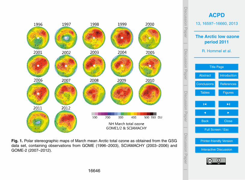
ACPD13, 16597–16660, 2013


R. Hommel et al.

Title Page



Tables Figures

J I

J I

Back Close

Full Screen / Esc



Discussion

Paper

|D

iscussionP

aper|

Discussion

Paper

|D

iscussionP

aper|

6 Rene Hommel et al.: The Arctic low ozone period 2011.

Fig. 1. Polar stereographic maps of March mean Arctic total ozone as obtained from the GSG data set, containing observations from GOME(1996 - 2003), SCIAMACHY (2003 - 2006) and GOME-2 (2007 - 2012).

ary) in 2007 and 2011. Minimum polar ozone was at a recordlow (close to 220 DU) in March 2011 and remained unusu-ally low until early April. Throughout March 2011 it was thelowest in the 15–year data record of the GSG data set.

The variability in Arctic ozone evident from the compactrelationship between the extra-tropical winter eddy heat flux,a measure of wave forcing of the winter residual circulation,and spring-to-fall polar cap ozone ratio, is shown in Fig. 3(Weber et al., 2011). This figure shows data from both hemi-spheres (triangles for SH, circles for NH). A spring-to-fallratio larger than one indicates that ozone transport outweighspolar ozone losses (typically in the NH) and smaller than onethat polar ozone loss dominates (typically in the SH). Plan-etary wave activity during Arctic winter-spring 2010/2011was among the lowest in the NH in the thirty years of satel-lite data, but still higher than typically seen in the SH in-cluding the heavily perturbed Antarctic ozone hole in winter

2002 (Richter et al., 2005; von Savigny et al., 2005a). As aresult, ozone transport from its source regions in the tropicalstratosphere into the mid- and high latitudes of the north-ern hemisphere was weaker in the second half of 2010 thanin other years and in the following winter 2010/2011, polarstratospheric temperatures were lower favouring conditionsfor large polar ozone losses. The Arctic winter 2009/2010,one year before, is located at the upper end of the range ofwinter planetary wave activity (Fig. 3). In that winter theBrewer-Dobson circulation was particularly strong (coincid-ing with an extremely negative Arctic Oscillation phase) withvery high ozone throughout the NH (Steinbrecht et al., 2011).

3.2 Arctic ozone in March 2010 and 2011

The consecutive winters 2010 and 2011 are good examplesof largely varying ozone levels over the Arctic. In winter-spring 2010, Arctic ozone was unusually high, whereas a

Fig. 1. Polar stereographic maps of March mean Arctic total ozone as obtained from the GSGdata set, containing observations from GOME (1996–2003), SCIAMACHY (2003–2006) andGOME-2 (2007–2012).

16646





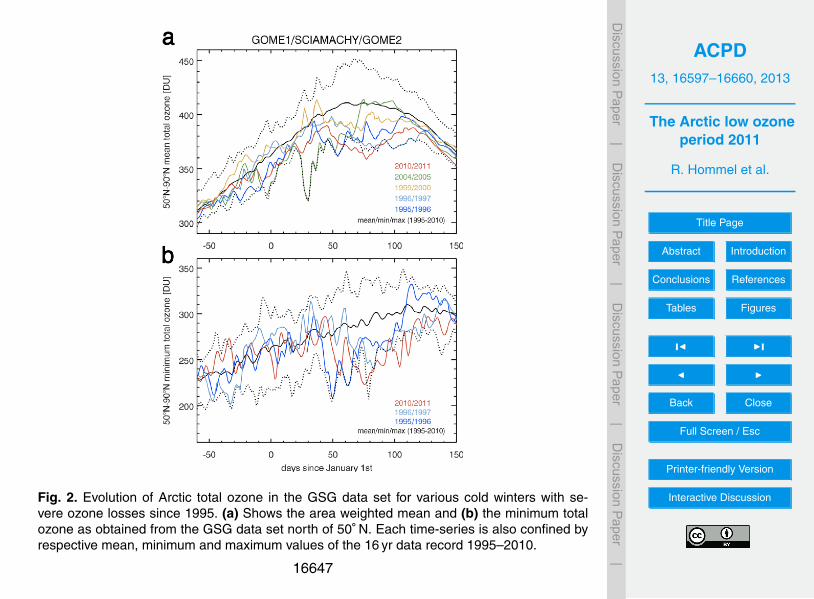
ACPD13, 16597–16660, 2013


R. Hommel et al.

Title Page



Tables Figures

J I

J I

Back Close

Full Screen / Esc



Discussion

Paper

|D

iscussionP

aper|

Discussion

Paper

|D

iscussionP

aper|

Fig. 2. Evolution of Arctic total ozone in the GSG data set for various cold winters with se-vere ozone losses since 1995. (a) Shows the area weighted mean and (b) the minimum totalozone as obtained from the GSG data set north of 50◦ N. Each time-series is also confined byrespective mean, minimum and maximum values of the 16 yr data record 1995–2010.

16647





ACPD13, 16597–16660, 2013


R. Hommel et al.

Title Page



Tables Figures

J I

J I

Back Close

Full Screen / Esc



Discussion

Paper

|D

iscussionP

aper|

Discussion

Paper

|D

iscussionP

aper|

Copernicus Publications

Bahnhofsallee 1e

37081 Göttingen

Germany

Martin Rasmussen (Managing Director)

Nadine Deisel (Head of Production/Promotion)

Contact

[email protected]

http://publications.copernicus.org

Phone +49-551-900339-50

Fax +49-551-900339-70

Legal Body

Copernicus Gesellschaft mbH

Based in Göttingen

Registered in HRB 131 298

County Court Göttingen

Tax Office FA Göttingen

USt-IdNr. DE216566440

Page 1/1

Fig. 3. Correlation between winter eddy heat flux and spring-to-fall ozone ratio over the polarcaps (update from Weber et al., 2011). Triangles are data from the SH; circles from the NH.

16648





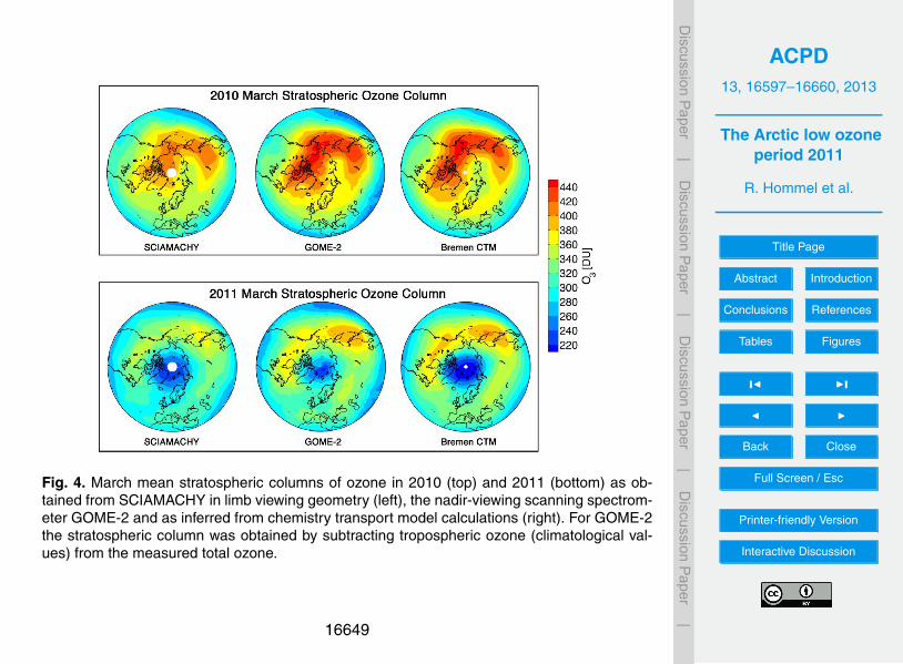
ACPD13, 16597–16660, 2013


R. Hommel et al.

Title Page



Tables Figures

J I

J I

Back Close

Full Screen / Esc



Discussion

Paper

|D

iscussionP

aper|

Discussion

Paper

|D

iscussionP

aper|


Bahnhofsallee 1e

37081 Göttingen

Germany



Contact

[email protected]


Phone +49-551-900339-50

Fax +49-551-900339-70

Legal Body


Based in Göttingen





Page 1/1

Fig. 4. March mean stratospheric columns of ozone in 2010 (top) and 2011 (bottom) as ob-tained from SCIAMACHY in limb viewing geometry (left), the nadir-viewing scanning spectrom-eter GOME-2 and as inferred from chemistry transport model calculations (right). For GOME-2the stratospheric column was obtained by subtracting tropospheric ozone (climatological val-ues) from the measured total ozone.

16649





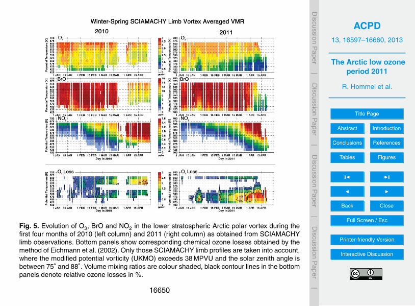
ACPD13, 16597–16660, 2013


R. Hommel et al.

Title Page



Tables Figures

J I

J I

Back Close

Full Screen / Esc



Discussion

Paper

|D

iscussionP

aper|

Discussion

Paper

|D

iscussionP

aper|


Bahnhofsallee 1e

37081 Göttingen

Germany



Contact

[email protected]


Phone +49-551-900339-50

Fax +49-551-900339-70

Legal Body


Based in Göttingen





Page 1/1

Fig. 5. Evolution of O3, BrO and NO2 in the lower stratospheric Arctic polar vortex during thefirst four months of 2010 (left column) and 2011 (right column) as obtained from SCIAMACHYlimb observations. Bottom panels show corresponding chemical ozone losses obtained by themethod of Eichmann et al. (2002). Only those SCIAMACHY limb profiles are taken into account,where the modified potential vorticity (UKMO) exceeds 38 MPVU and the solar zenith angle isbetween 75◦ and 88◦. Volume mixing ratios are colour shaded, black contour lines in the bottompanels denote relative ozone losses in %.

16650





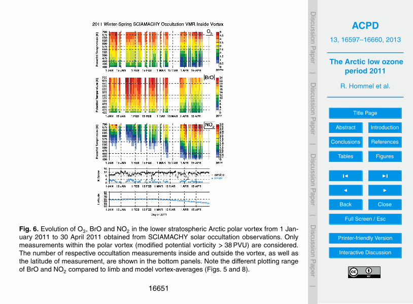
ACPD13, 16597–16660, 2013


R. Hommel et al.

Title Page



Tables Figures

J I

J I

Back Close

Full Screen / Esc



Discussion

Paper

|D

iscussionP

aper|

Discussion

Paper

|D

iscussionP

aper|


tropic ozone loss estimate, developed to infer the strengthof the chemically-induced polar ozone destruction indepen-dently from reasons related to the dynamics of the atmo-sphere, is examined in more detail in Section 3.8.

By comparison, in the warmer and weaker Arctic vor-tex 2010 ozone losses barely exceeded 20 % below 550 K.Above the 550 K isentropic surface, however, we infer anozone depletion of up to 40 % during spring 2010 (relativeto values at first day of the year). The slower descent ofair in the strong vortex 2010/2011 implies that this upperlayer of ozone depletion is found at higher altitudes as in2010. Above the regions where halogen driven catalytic cy-cles remove ozone, NOx (NO+NO2) photochemistry is pre-dominantly responsible for ozone depletion (Osterman et al.,1997). This process is stronger during warm winter yearswhen the vortex is weaker because less denitrification onfewer PSCs is taking place, air from the upper stratosphere isfaster descending and the lateral mixing of NO2-rich air frommid-latitudes is more likely than in cold winter-spring peri-ods when vortex mixing-barrier is much stronger (Rosenfieldet al., 1994; Konopka et al., 2007). As shown in Sonkaewet al. (2013) these NOx driven catalytic ozone losses abovethe 550 K isentropic level are frequently observed in the Arc-tic polar stratosphere in late spring.

Manney et al. (2011) reported chemically induced ozonelosses on the order of at least 2.5 ppmv between 470 Kand 550 K by end of March 2011 from Lagrangian chem-ical transport model studies and ozone measurements fromMLS/Aura and the Match network of ozone sondes. Thisnumber is consistent with ours, which is 2.5-3 ppmv atthe end of March. Our SCIAMACHY based loss estimate,however, is slightly (0.5 ppmv) lower above 525 K as thatof Manney et al. (2011). The onset of the catalytic ozonedestruction occurs around 1 February 2011 in both studies.Sinnhuber et al. (2011) inferred column ozone losses of upto 120 DU towards end of April 2011 from MIPAS obser-vations. These observations are principally confirmed bycorresponding model simulations conducted with an isen-tropic CTM of very similar set-up as ours used in thisstudy (Sinnhuber et al., 2003; Aschmann et al., 2011), butdifferently initialized and driven by meteorology from theECMWF operational analysis. Sinnhuber et al. (2011) alsoshowed MIPAS ozone at the 475 K isentropic surface re-duced to 1.5 ppmv in early April 2011, which is rather atthe upper end of our estimate. Arnone et al. (2012) reportedMIPAS based vortex-averaged ozone reductions down to 0.6ppmv in early April 2011 at 18 km (∼430 K isentrope), ingood agreement with our data. Their corresponding ozonelosses are also matching our estimates, although based ona different method, taking correlative MIPAS N2O observa-tions into account.

Fig. 6. Evolution of O3, BrO and NO2 in the lower stratosphericArctic polar vortex from 01 January 2011 to 30 April 2011 ob-tained from SCIAMACHY solar occultation observations. Onlymeasurements within the polar vortex (modified potential vorticity> 38 PVU) are considered. The number of respective occultationmeasurements inside and outside the vortex, as well as the latitudeof measurement, are shown in the bottom panels. Note the differ-ent plotting range of BrO and NO2 compared to limb and modelvortex-averages (Fig. 5 and Fig. 8).

3.4 SCIAMACHY solar occultation measurements: O3,NO2 and BrO

In order to complement our results obtained from the limb-scatter measurements shown in Fig. 5, we also retrieved O3,BrO, and NO2 profiles from SCIAMACHY solar occultationmeasurements (Fig. 6). As for limb profiles, in our analy-sis we consider only those occultation profiles located withinthe vortex. Since solar occultation measurements were per-formed at different local time (sunset around 18:00, com-pared to morning local time around 10:00 for limb geome-try), respective vortex-averages are obtained from differentgeolocations compared to the limb data. This is demon-

Fig. 6. Evolution of O3, BrO and NO2 in the lower stratospheric Arctic polar vortex from 1 Jan-uary 2011 to 30 April 2011 obtained from SCIAMACHY solar occultation observations. Onlymeasurements within the polar vortex (modified potential vorticity > 38 PVU) are considered.The number of respective occultation measurements inside and outside the vortex, as well asthe latitude of measurement, are shown in the bottom panels. Note the different plotting rangeof BrO and NO2 compared to limb and model vortex-averages (Figs. 5 and 8).

16651





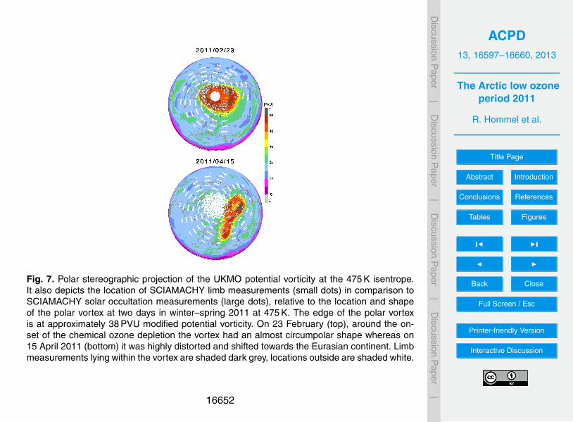
ACPD13, 16597–16660, 2013


R. Hommel et al.

Title Page



Tables Figures

J I

J I

Back Close

Full Screen / Esc



Discussion

Paper

|D

iscussionP

aper|

Discussion

Paper

|D

iscussionP

aper|


Fig. 7. Polar stereographic projection of the UKMO potential vor-ticity at the 475 K isentrope. It also depicts the location of SCIA-MACHY limb measurements (small dots) in comparison to SCIA-MACHY solar occultation measurements (large dots), relative to thelocation and shape of the polar vortex at two days in winter-spring2011 at 475 K. The edge of the polar vortex is at approximately38 PVU modified potential vorticity. On 23 February (top), aroundthe onset of the chemical ozone depletion the vortex had an almostcircumpolar shape whereas on 15 April 2011 (bottom) it was highlydistorted and shifted towards the Eurasian continent. Limb mea-surements lying within the vortex are shaded dark gray, locationsoutside are shaded white.

mation reaction of bromine nitrate (BrONO2) towards BrOdue to the lower NO2 mixing ratios.

With the return of sunlight, polar NO2 is reconverted fromits reservoir species N2O5. Although the timing of the onsetof this photochemical regeneration is well reproduced by the

CTM, springtime vortex-averaged NO2 levels are underes-timated. This underestimation results from a generally lowbias in model NO2, so that lateral mixing of NO2-rich airfrom mid-latitudes (Noxon cliff; Noxon, 1979) cannot ac-count for restoring springtime polar NO2 levels to the sameextent as seen in the limb vortex-averages. In April 2011,the CTM shows approximately half of the NO2 measured bySCIAMACHY limb, in April 2010 the low bias is less dis-tinct and in the order of a third.

3.5.2 Modelled ozone losses

In the model, polar ozone losses are quantified as thedifference between the modelled chemically fully interac-tive ozone and a quasi-passive ozone tracer (LINOZ; lin-earised chemistry without heterogeneous reactions). Result-ing losses are in good agreement with the estimate fromSCIAMACHY limb measurements below the 550 K isen-tropic surface. Relative to SCIAMACHY, modelled ozonelosses are approximately 10 % overestimated in April 2011.In 2010, we find rather a slightly underestimation of the mod-elled induced losses in that region. The overestimation ofthe 2011 loss is in the same range as the ones reported bySingleton et al. (2007) from SLIMCAT CTM model stud-ies of the so far most severe Arctic ozone losses observedin winter-spring 2004/2005. They compared to loss esti-mates from various satellite instruments based on the passivetracer subtraction method and argued that mainly samplingdifferences between the data sets may have led to overes-timated model losses. The differences between the ozoneloss inferred from our CTM simulations and the estimatesfrom SCIAMACHY limb measurements are also partly at-tributable to small differences in the vortex sampling of thetwo data sets. Additionally, we cannot rule out that deficitsin the model treatment of PSCs and accompanied effects ofheterogenous chemistry on those particles may play a sub-stantial role in the overestimation of ozone depletion, in par-ticular during spring.

One striking difference between ozone losses from SCIA-MACHY and the CTM is the absence of the NOx drivenozone decomposition layer above 550 K in the model. Thisis not an effect of the general underestimation of polar NO2

in the CTM, it is rather an inherent effect of the approachused to infer ozone losses in the model. The loss due to NOx

is parameterized in the LINOZ scheme and thus impacts thelinearized ozone tracer which represents the reference of themodel’s loss estimate. Consequently, this layer is not de-ducible from the approach used here.

The apparent ozone loss in mid-January 2011 seen in theSCIAMACHY limb estimate (Fig. 5, bottom right panel),however, is also not inferable from model results since a re-spective decrease of ozone mixing ratios is not seen in themodelled ozone time-series. In Section 3.8.3 we investigatethis behaviour in more detail.

Fig. 7. Polar stereographic projection of the UKMO potential vorticity at the 475 K isentrope.It also depicts the location of SCIAMACHY limb measurements (small dots) in comparison toSCIAMACHY solar occultation measurements (large dots), relative to the location and shapeof the polar vortex at two days in winter–spring 2011 at 475 K. The edge of the polar vortexis at approximately 38 PVU modified potential vorticity. On 23 February (top), around the on-set of the chemical ozone depletion the vortex had an almost circumpolar shape whereas on15 April 2011 (bottom) it was highly distorted and shifted towards the Eurasian continent. Limbmeasurements lying within the vortex are shaded dark grey, locations outside are shaded white.

16652





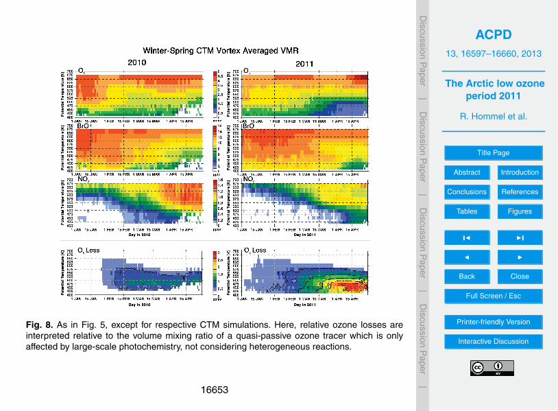
ACPD13, 16597–16660, 2013


R. Hommel et al.

Title Page



Tables Figures

J I

J I

Back Close

Full Screen / Esc



Discussion

Paper

|D

iscussionP

aper|

Discussion

Paper

|D

iscussionP

aper|

Rene Hommel et al.: The Arctic low ozone period 2011. 13

Fig. 8. As in Fig. 5, except for respective CTM simulations. Here, relative ozone losses are interpreted relative to the volume mixing ratio ofa quasi-passive ozone tracer which is only affected by large-scale photochemistry, not considering heterogeneous reactions.

3.6 SCIAMACHY limb observations of PSCs

The meteorological conditions in the 2011 Arctic winter-spring polar vortex favoured the formation of PSCs. Fig. 9shows the temporal evolution of the daily mean PSC occur-rence rate (left panel) and daily averaged PSC altitude (rightpanel) - both in the 60◦N - 80◦N latitude range - for sev-eral Arctic winters including 2010/2011 from January 1st toApril 1st. The PSC occurrence rate is given by the ratio ofthe number of SCIAMACHY measurements with PSC de-tections and the total number of measurements - on a givenday and within a certain latitude range.

In January 2010 a very strong PSC occurrence duringan approximately one-month period, from mid-Decemberto mid-January seen in Fig. 9, was observed also by thespace-borne CALIOP (Cloud-Aerosol Lidar with Orthog-onal Polarisation) instrument onboard CALIPSO (Cloud-

Aerosol Lidar and Infrared Pathfinder Satellite Observations)as shown in Khosrawi et al. (2011) and Pitts et al. (2011).The total supply of PSCs during the entire winter-spring pe-riod was even stronger in 2011. From SCIAMACHY limb-scatter observations we infer that the PSC occurrence ratein 2010 was some 20 % larger than in 2011, but only dur-ing a relatively short period, that ended at the beginning ofFebruary 2010. In contrast, during the 2010/2011 season,PSCs were formed from the end of December 2010 and werepresent over the pole until the 18th of March (Khosrawi et al.,2012).

The 2011 SCIAMACHY PSC record shows three periodsof maximized PSC formation - at the beginning of January,from 18 January to 1 February and a long-lasting period af-ter the 8th of February. During this third period, the PSCsoccurrence rate steadily increased, until a maximum was ob-served on 22 March 2011. In comparison, CALIOP detected

Fig. 8. As in Fig. 5, except for respective CTM simulations. Here, relative ozone losses areinterpreted relative to the volume mixing ratio of a quasi-passive ozone tracer which is onlyaffected by large-scale photochemistry, not considering heterogeneous reactions.

16653





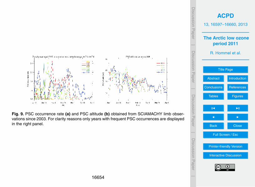
ACPD13, 16597–16660, 2013


R. Hommel et al.

Title Page



Tables Figures

J I

J I

Back Close

Full Screen / Esc



Discussion

Paper

|D

iscussionP

aper|

Discussion

Paper

|D

iscussionP

aper|


Fig. 9. PSC occurrence rate (a) and PSC altitude (b) obtained from SCIAMACHY limb observations since 2003. For clarity reasons onlyyears with frequent PSC occurrences are displayed in the right panel.

four PSC periods, starting earlier on 23 December 2010. Notexactly similar to the periods seen by SCIAMACHY, butlargely overlapping. A similar increase during March wasalso observed in 2005, when the so far largest total ozonemass loss was observed (Sonkaew et al., 2013). In 2005,however, most PSCs were formed during the last days ofJanuary - at comparable rates as in 2008 and 2010. In thelatter two years, however, respective periods lasted only afew days, hence were distinctly different from the conditionsseen in 2011 and 2005.

In this context, we also have to keep in mind that the vor-tex sampling of SCIAMACHY limb measurements in Jan-uary may be quite poor, and the variability in PSC occur-rence rates seen in Fig. 9 in January may be partly explainedby this.

The right panel of Fig. 9 impressively demonstrates thePSC descent during the course of winter-spring. This descentis not only attributed to particle sedimentation, to a large ex-tent it reflects the descent of the lower stratospheric temper-ature minimum, as has been demonstrated for the southernhemisphere by von Savigny et al. (2005b). PSC altitudes de-rived from SCIAMACHY correspond to PSC top altitudes,not to centroid altitudes. The cloud thickness cannot be in-ferred using the method applied.

Informations about the composition of the observed PSCscan be obtained from measurements by the CALIOP in-strument onboard CALIPSO. According to CALIOP, the2009/2010 PSC season stated with the formation of predom-inantly type I PSCs, that diverged more and more over timeinto the formation of type II (ice) particles. In contrast, dur-ing the whole 2010/2011 PSC season, type II clouds werealways found together with type Ia (NAT) and type Ib (STS)clouds (Khosrawi et al., 2012). However, from such infor-mations alone one cannot state which PSC type is giving

rise to particular features or characteristics that are seen inthe vortex-average ozone time-series. But PSC observationscorrelate well with certain aspects seen in the polar HNO3

and N2O time-series as measured by other instruments, forinstance MLS/Aura or SMR/Odin (Khosrawi et al., 2011,2012; Manney et al., 2011). Khosrawi et al. (2011) showedthat the so far largest denitrification over the last decade inwinter-spring 2009/2010 emerged from an extended forma-tion of solid particles (NAT/ice) in early winter. In winter-spring 2011, the overall denitrification was even more pro-nounced than in the winter before. It lasted much longerover four month and developed rather continuously, in con-trast to the rather short one-month period of cold tempera-tures in 2010 (Khosrawi et al., 2012). There is no doubt thatdenitrification played a large role for the ozone losses 2011,however, recently Strahan et al. (2013) argued that the unex-pected dynamical situation of the polar stratosphere may beaccountable for around one-third of the ozone destroyed inthe Arctic vortex in March and April 2011.

In 2005, when the so far largest Arctic chemical ozonelosses were observed (Manney et al., 2006, 2011; Sonkaewet al., 2013), a temporal evolution of PSC occurrence is seenwhich is very similar to that in 2011.

After a strong event of PSC formation around 30 January2005, PSCs were further formed over large areas over theArctic, steadily increasing until the end of February when afinal warming halted PSC existence. Based on model studies,Feng et al. (2007) argued that during the course of the 2005winter PSCs were mainly composed of type I (STS/NAT),whereby the strong PSC formation around 30 January 2005is attributable to type I and II PSCs in approximately equalmeasure.

Fig. 9. PSC occurrence rate (a) and PSC altitude (b) obtained from SCIAMACHY limb obser-vations since 2003. For clarity reasons only years with frequent PSC occurrences are displayedin the right panel.

16654





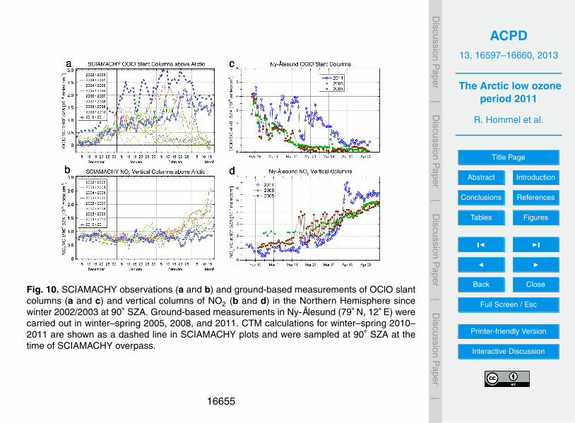
ACPD13, 16597–16660, 2013


R. Hommel et al.

Title Page



Tables Figures

J I

J I

Back Close

Full Screen / Esc



Discussion

Paper

|D

iscussionP

aper|

Discussion

Paper

|D

iscussionP

aper|


Fig. 10. SCIAMACHY observations (a and b) and ground-based measurements of OClO slant columns (a and c) and vertical columns ofNO2 (b and d) in the Northern Hemisphere since winter 2002/2003 at 90◦ SZA. Ground-based measurements in Ny-Alesund (79◦N, 12◦E)were carried out in winter-spring 2005, 2008, and 2011. CTM calculations for winter-spring 2010 - 2011 are shown as a dashed line inSCIAMACHY plots and were sampled at 90◦ SZA at the time of SCIAMACHY overpass.

Fig. 11. Daily maps of total ozone measured by GOME-2 between 20 and 31 January 2011. On 21 January 2011 column ozone wassubstantially lowered by more than 70 DU over Central Siberia north of Sakhalin, and was moving westwards to the Ural region. After 28January 2011 the area of low ozone moves eastward and dissolves at approximately 90 - 100◦E / 60◦N on 30 January.

before low column ozone was observed over Central Siberianorth of Sakhalin island. This area of low ozone was cen-tered at approximately 140◦E / 63◦N and had an initial ex-tent of about 2000×1000 km in longitude and latitude (or1.4×106 km2). In the following six days the low ozone areaapproximately doubled in size and moved westwards across

the Ural region. On 28 January it moved a few degrees east-wards towards Central Siberia, where it dissolved two dayslater. Thereafter, Arctic ozone replenished temporarily untilaround the 6th February. Vortex ozone again declined andremained low for the following almost three month, accord-ing to the SCIAMACHY limb vortex-avereaged O3 mixing-

Fig. 10. SCIAMACHY observations (a and b) and ground-based measurements of OClO slantcolumns (a and c) and vertical columns of NO2 (b and d) in the Northern Hemisphere sincewinter 2002/2003 at 90◦ SZA. Ground-based measurements in Ny-Ålesund (79◦ N, 12◦ E) werecarried out in winter–spring 2005, 2008, and 2011. CTM calculations for winter–spring 2010–2011 are shown as a dashed line in SCIAMACHY plots and were sampled at 90◦ SZA at thetime of SCIAMACHY overpass.

16655





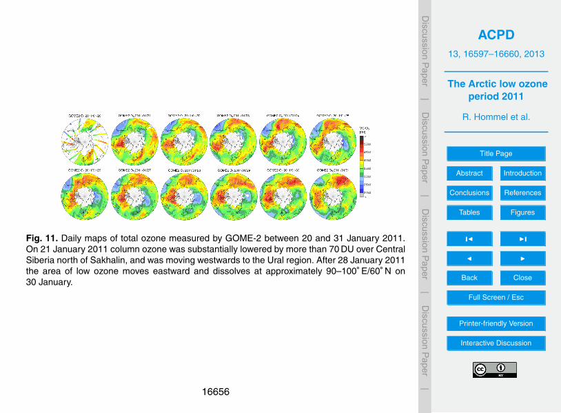
ACPD13, 16597–16660, 2013


R. Hommel et al.

Title Page



Tables Figures

J I

J I

Back Close

Full Screen / Esc



Discussion

Paper

|D

iscussionP

aper|

Discussion

Paper

|D

iscussionP

aper|


Fig. 10. SCIAMACHY observations (a and b) and ground-based measurements of OClO slant columns (a and c) and vertical columns ofNO2 (b and d) in the Northern Hemisphere since winter 2002/2003 at 90◦ SZA. Ground-based measurements in Ny-Alesund (79◦N, 12◦E)were carried out in winter-spring 2005, 2008, and 2011. CTM calculations for winter-spring 2010 - 2011 are shown as a dashed line inSCIAMACHY plots and were sampled at 90◦ SZA at the time of SCIAMACHY overpass.

Fig. 11. Daily maps of total ozone measured by GOME-2 between 20 and 31 January 2011. On 21 January 2011 column ozone wassubstantially lowered by more than 70 DU over Central Siberia north of Sakhalin, and was moving westwards to the Ural region. After 28January 2011 the area of low ozone moves eastward and dissolves at approximately 90 - 100◦E / 60◦N on 30 January.

before low column ozone was observed over Central Siberianorth of Sakhalin island. This area of low ozone was cen-tered at approximately 140◦E / 63◦N and had an initial ex-tent of about 2000×1000 km in longitude and latitude (or1.4×106 km2). In the following six days the low ozone areaapproximately doubled in size and moved westwards across

the Ural region. On 28 January it moved a few degrees east-wards towards Central Siberia, where it dissolved two dayslater. Thereafter, Arctic ozone replenished temporarily untilaround the 6th February. Vortex ozone again declined andremained low for the following almost three month, accord-ing to the SCIAMACHY limb vortex-avereaged O3 mixing-

Fig. 11. Daily maps of total ozone measured by GOME-2 between 20 and 31 January 2011.On 21 January 2011 column ozone was substantially lowered by more than 70 DU over CentralSiberia north of Sakhalin, and was moving westwards to the Ural region. After 28 January 2011the area of low ozone moves eastward and dissolves at approximately 90–100◦ E/60◦ N on30 January.

16656





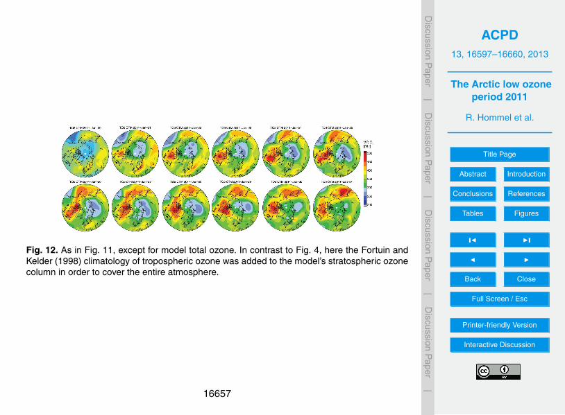
ACPD13, 16597–16660, 2013


R. Hommel et al.

Title Page



Tables Figures

J I

J I

Back Close

Full Screen / Esc



Discussion

Paper

|D

iscussionP

aper|

Discussion

Paper

|D

iscussionP

aper|


Bahnhofsallee 1e

37081 Göttingen

Germany



Contact

[email protected]


Phone +49-551-900339-50

Fax +49-551-900339-70

Legal Body


Based in Göttingen





Page 1/1

Fig. 12. As in Fig. 11, except for model total ozone. In contrast to Fig. 4, here the Fortuin andKelder (1998) climatology of tropospheric ozone was added to the model’s stratospheric ozonecolumn in order to cover the entire atmosphere.

16657





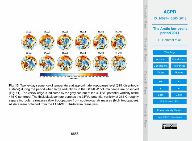
ACPD13, 16597–16660, 2013


R. Hommel et al.

Title Page



Tables Figures

J I

J I

Back Close

Full Screen / Esc



Discussion

Paper

|D

iscussionP

aper|

Discussion

Paper

|D

iscussionP

aper|


Bahnhofsallee 1e

37081 Göttingen

Germany



Contact

[email protected]


Phone +49-551-900339-50

Fax +49-551-900339-70

Legal Body


Based in Göttingen





Page 1/1

Fig. 13. Twelve day sequence of temperature at approximate tropopause level (315 K isentropicsurface) during the period when large reductions in the GOME-2 column ozone are observed(Fig. 11). The vortex edge is indicated by the grey contour of the 38 PVU potential vorticity at the475 K isentrope. The thick black contour denotes the 3 PVU potential vorticity at 315 K, roughlyseparating polar airmasses (low tropopause) from subtropical air masses (high tropopause).All data were obtained from the ECMWF ERA-Interim reanalysis.

16658





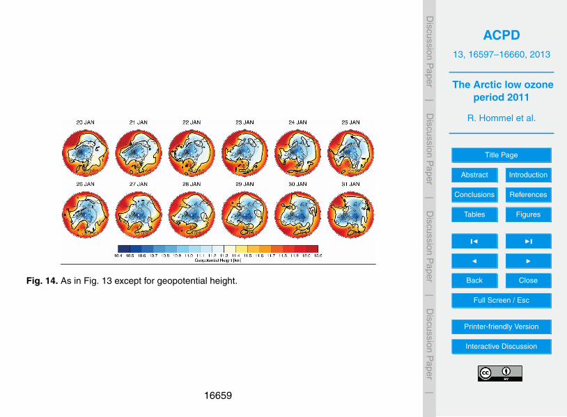
ACPD13, 16597–16660, 2013


R. Hommel et al.

Title Page



Tables Figures

J I

J I

Back Close

Full Screen / Esc



Discussion

Paper

|D

iscussionP

aper|

Discussion

Paper

|D

iscussionP

aper|


Bahnhofsallee 1e

37081 Göttingen

Germany



Contact

[email protected]


Phone +49-551-900339-50

Fax +49-551-900339-70

Legal Body


Based in Göttingen





Page 1/1

Fig. 14. As in Fig. 13 except for geopotential height.

16659





ACPD13, 16597–16660, 2013


R. Hommel et al.

Title Page



Tables Figures

J I

J I

Back Close

Full Screen / Esc



Discussion

Paper

|D

iscussionP

aper|

Discussion

Paper

|D

iscussionP

aper|


Fig. 15. As in Fig. 13 except for pressure at the 350 K isentropic surface.

comparably small ozone mini-hole is seen in GOME-2 to-tal ozone between 27 and 30 January 2011. In the relativecoarse resolved CTM (resolution 2.5◦ in latitude, 3.75◦ inlongitude) this OMH is not well reproduced. Only on 30 Jan-uary 2011 the OMH is apparent in the CTM, a few degreesshifted to the Northwest (Fig. 12).

3.8.3 Modelling the January 2011 Arctic low ozone event

As shown in Fig. 12, the CTM largely reproduces the day-to-day variability of stratospheric ozone over the Arctic. Onlysmall-scale synoptic features like the Scandinavian ozonemini-hole around the 28th of January 2011 are not adequatelyresolved. Also the magnitude of thinning the ozone columnduring the OMH-like situation is not captured well comparedto GOME-2 observations. GOME-2 shows ozone as lowas 200 DU on several days near the polar night blind spot,whereas the model’s total ozone is not lower than 250 DU.Partly, this deficit is attributable to an approximated tropo-spheric contribution to the total ozone column.

A respective reduction in the height-resolved and vortex-averaged time-series of modelled Arctic ozone 2011 (Fig. 8)is not seen, in contrast to the vortex-average constructed fromSCIAMACHY limb ozone profiles (Fig. 5). Although modeldata have been written at local times of SCIAMACHY over-passes and were sampled in similar manner as limb profilesin order to construct vortex-averages, i.e. grid cells lyingwithin the vortex where modified PV > 38 PVU but south of80◦N, exhibiting SZAs < 88◦, certain differences betweenthe areas of the vortex covered by these two sampling meth-ods persist. This may lead to the effect that in the modelsmall-scale drops in the screened vortex O3 mixing ratio aresimply averaged out.

On the other hand, model equations are solved on isen-tropes. In the polar stratosphere isentropes are invariant toadiabatic processes in the tropopause region, so that a ”thin-ning effect” in ozone mixing ratios above tropopause eleva-tions is not apparent in the model vortex-average as long asthe meridional divergence of ozone containing air out of thecolumn is small. When the vortex-average is inferred frombehaviour number densities, the ”thinning effect” becomesapparent (not shown) and is in the order of 35 % below the475 K isentrope, relative to average values in the undistortedvortex before and after this episode. This effect is approxi-mately twice as large in the limb vortex-average (Sec. 3.3.2).Furthermore, in the model this ”thinning effect” in the ozonenumber density does not extend well into the stratosphere.Projected on geometric altitudes, this effect disappears atleast 2 km below the regions in respective limb profiles.Whether meridional divergence of ozone containing air outof the column is underestimated in the CTM and better re-solved in the vortex-average from limb measured ozone pro-files, cannot be satisfactorily answered yet. However, suchan underestimation is not unlikely because the model runsin a relatively coarse horizontal resolution so that numericaldiffusion may play a role here even if the model’s driving me-teorology (ERA-Interim) is reproducing well the dynamicalaspects of the OMH situation.

3.8.4 Implications for vortex-average ozone loss estimates

What do these conclusions mean for the vortex-averageinferred from SCIAMACHY limb measurements and themodel during time of the OMH-like situation in the Arcticstratosphere between 21 and 29 January 2011?

Fig. 15. As in Fig. 13 except for pressure at the 350 K isentropic surface.

16660





Chemical composition and severe ozone loss derived from SCIAMACHY and GOME-2 observations during Arctic winter 2010/2011 in comparisons to Arctic winters in the past

Documents