Chef: a cheap and fast pipeline for iteratively cleaning label uncertainties Yinjun Wu University of Pennsylvania [email protected] James Weimer University of Pennsylvania [email protected] Susan B. Davidson University of Pennsylvania [email protected] ABSTRACT High-quality labels are expensive to obtain for many machine learn- ing tasks, such as medical image classification tasks. Therefore, probabilistic (weak) labels produced by weak supervision tools are used to seed a process in which influential samples with weak labels are identified and cleaned by several human annotators to improve the model performance. To lower the overall cost and computa- tional overhead of this process, we propose a solution called Chef (CHEap and Fast label cleaning), which consists of the following three components. First, to reduce the cost of human annotators, we use Infl, which prioritizes the most influential training samples for cleaning and provides cleaned labels to save the cost of one human annotator. Second, to accelerate the sample selector phase and the model constructor phase, we use Increm-Infl to incrementally pro- duce influential samples, and DeltaGrad-L to incrementally update the model. Third, we redesign the typical label cleaning pipeline so that human annotators iteratively clean smaller batch of samples rather than one big batch of samples. This yields better overall model performance and enables possible early termination when the expected model performance has been achieved. Extensive ex- periments show that our approach gives good model prediction performance while achieving significant speed-ups. PVLDB Reference Format: Yinjun Wu, James Weimer, and Susan B. Davidson. Chef: a cheap and fast pipeline for iteratively cleaning label uncertainties. PVLDB, 14(1): XXX-XXX, 2020. doi:XX.XX/XXX.XX PVLDB Artifact Availability: The source code, data, and/or other artifacts have been made available at http://vldb.org/pvldb/format_vol14.html. 1 INTRODUCTION There is a general consensus that the success of advanced machine learning models depends on the availability of extremely large training sets with high-quality labels. Unfortunately, obtaining high-quality labels may be prohibitively expensive. For example, labeling medical images typically requires the effort of experts with domain knowledge. To produce labels at large scale with low cost, weak supervision tools—such as Snorkel [33]—can be used to automatically generate probabilistic labels (or weak labels) for unlabeled training samples by leveraging labeling functions [33]. This work is licensed under the Creative Commons BY-NC-ND 4.0 International License. Visit https://creativecommons.org/licenses/by-nc-nd/4.0/ to view a copy of this license. For any use beyond those covered by this license, obtain permission by emailing [email protected]. Copyright is held by the owner/author(s). Publication rights licensed to the VLDB Endowment. Proceedings of the VLDB Endowment, Vol. 14, No. 1 ISSN 2150-8097. doi:XX.XX/XXX.XX Figure 1: The iterative pipeline of cleaning uncertainties from the labels of training set. It has been shown in [2, 29, 36], however, that imperfect labeling functions can produce inferior probabilistic labels, thus hurting the downstream model quality. Therefore, it is necessary to perform additional cleaning operations to clean such label uncertainties [29]. The label cleaning process is typically iterative [21, 25], and re- quires multiple rounds (see Figure 1, loop labeled 1 ). First, given a cleaning budget , the top- influential training samples with probabilistic labels are selected (the sample selector phase). Second, for those selected samples, cleaned labels are provided by human annotators (the annotation phase). Third, the ML model is calcu- lated using the updated training set (the model constructor phase), and returned to the user. If the resulting model performance is not good enough, the process is repeated with an additional budget ′ . Otherwise, it is deployed. Note that since each of these phases may be performed repeatedly, it is important that they be as efficient as possible. It is also noteworthy that for some applications—such as the medical image classification task—it is essential to have multi- ple human annotators for label cleaning to alleviate their labeling errors [16] in the annotation phase, thus incurring substantial time overhead and financial cost. In this paper, we propose a solu- tion called Chef (CHEap and Fast label cleaning), to reduce the time overhead and cost of the label cleaning pipeline and simultaneously enhance the overall model performance. De- tails of the overall design of Chef are given next. Sample selector phase. Finding the most influential training samples can be done with several different influence measures, e.g., the influence function [20], the Data Shapley values [17], the noisy label detection algorithms [9, 15], the active learning technique [35] or using a bi-level optimization solution [42]. Unfortunately, these do not work well for cleaning weak labels. We therefore develop a variant of the influence function called Infl which can simultaneously detect the most influential samples and suggest arXiv:2107.08588v1 [cs.DB] 19 Jul 2021

Welcome message from author
This document is posted to help you gain knowledge. Please leave a comment to let me know what you think about it! Share it to your friends and learn new things together.
Transcript

Chef: a cheap and fast pipeline for iteratively cleaning labeluncertainties
Yinjun Wu
University of Pennsylvania
James Weimer
University of Pennsylvania
Susan B. Davidson
University of Pennsylvania
ABSTRACTHigh-quality labels are expensive to obtain for many machine learn-
ing tasks, such as medical image classification tasks. Therefore,
probabilistic (weak) labels produced by weak supervision tools are
used to seed a process in which influential samples with weak labels
are identified and cleaned by several human annotators to improve
the model performance. To lower the overall cost and computa-
tional overhead of this process, we propose a solution called Chef
(CHEap and Fast label cleaning), which consists of the following
three components. First, to reduce the cost of human annotators, we
use Infl, which prioritizes the most influential training samples for
cleaning and provides cleaned labels to save the cost of one human
annotator. Second, to accelerate the sample selector phase and the
model constructor phase, we use Increm-Infl to incrementally pro-
duce influential samples, and DeltaGrad-L to incrementally update
the model. Third, we redesign the typical label cleaning pipeline so
that human annotators iteratively clean smaller batch of samples
rather than one big batch of samples. This yields better overall
model performance and enables possible early termination when
the expected model performance has been achieved. Extensive ex-
periments show that our approach gives good model prediction
performance while achieving significant speed-ups.
PVLDB Reference Format:Yinjun Wu, James Weimer, and Susan B. Davidson. Chef: a cheap and fast
pipeline for iteratively cleaning label uncertainties. PVLDB, 14(1):
XXX-XXX, 2020.
doi:XX.XX/XXX.XX
PVLDB Artifact Availability:The source code, data, and/or other artifacts have been made available at
http://vldb.org/pvldb/format_vol14.html.
1 INTRODUCTIONThere is a general consensus that the success of advanced machine
learning models depends on the availability of extremely large
training sets with high-quality labels. Unfortunately, obtaining
high-quality labels may be prohibitively expensive. For example,
labeling medical images typically requires the effort of experts
with domain knowledge. To produce labels at large scale with low
cost, weak supervision tools—such as Snorkel [33]—can be used
to automatically generate probabilistic labels (or weak labels) forunlabeled training samples by leveraging labeling functions [33].
This work is licensed under the Creative Commons BY-NC-ND 4.0 International
License. Visit https://creativecommons.org/licenses/by-nc-nd/4.0/ to view a copy of
this license. For any use beyond those covered by this license, obtain permission by
emailing [email protected]. Copyright is held by the owner/author(s). Publication rights
licensed to the VLDB Endowment.
Proceedings of the VLDB Endowment, Vol. 14, No. 1 ISSN 2150-8097.
doi:XX.XX/XXX.XX
Figure 1: The iterative pipeline of cleaning uncertaintiesfrom the labels of training set.
It has been shown in [2, 29, 36], however, that imperfect labeling
functions can produce inferior probabilistic labels, thus hurting the
downstream model quality. Therefore, it is necessary to perform
additional cleaning operations to clean such label uncertainties [29].
The label cleaning process is typically iterative [21, 25], and re-
quires multiple rounds (see Figure 1, loop labeled 1 ). First, given
a cleaning budget 𝐵, the top-𝐵 influential training samples with
probabilistic labels are selected (the sample selector phase). Second,for those selected samples, cleaned labels are provided by human
annotators (the annotation phase). Third, the ML model is calcu-
lated using the updated training set (the model constructor phase),and returned to the user. If the resulting model performance is not
good enough, the process is repeated with an additional budget 𝐵′.Otherwise, it is deployed. Note that since each of these phases may
be performed repeatedly, it is important that they be as efficient as
possible. It is also noteworthy that for some applications—such as
the medical image classification task—it is essential to have multi-
ple human annotators for label cleaning to alleviate their labeling
errors [16] in the annotation phase, thus incurring substantial time
overhead and financial cost. In this paper, we propose a solu-tion called Chef (CHEap and Fast label cleaning), to reducethe time overhead and cost of the label cleaning pipeline andsimultaneously enhance the overallmodel performance. De-tails of the overall design of Chef are given next.
Sample selector phase. Finding the most influential training
samples can be done with several different influence measures, e.g.,
the influence function [20], the Data Shapley values [17], the noisy
label detection algorithms [9, 15], the active learning technique
[35] or using a bi-level optimization solution [42]. Unfortunately,
these do not work well for cleaning weak labels. We therefore
develop a variant of the influence function called Infl which can
simultaneously detect the most influential samples and suggest
arX
iv:2
107.
0858
8v1
[cs
.DB
] 1
9 Ju
l 202
1

cleaned labels. One key technical challenge in the efficient imple-
mentation of Infl concerns the explicit evaluation of gradients on
every training sample.Weaddress this challenge by developingIncrem-Infl, which removes uninfluential training samplesearly and can thus incrementally recommend themost influ-ential training samples to human annotators.
Human annotation phase. After influential samples are selected,
the next step is for human annotators to clean the labels of those
samples. Recall thatmultiple human annotators may be used to inde-
pendently label each training sample, and inconsistencies between
the labels are resolved, e.g., by majority vote [16]. To reduce thecost of the human annotation phase, we consider the sug-gested clean labels from the sample selector phase as one al-ternative labeler, which can be combined with results pro-vided by the human annotators to reduce annotation cost.
Model constructor phase. In previous work [40], we developed
a provenance-based algorithm called DeltaGrad for incrementallyupdating model parameters after the deletion or addition of a small
subset of training samples, and showed that it was significantly
faster than recalculating the model from scratch. Since the result
of the human annotation phase can be regarded as the deletion of
top-𝐵 samples with probabilistic labels, and insertion of those same
samples with cleaned labels, we can adapt DeltaGrad for this setting.
This algorithm is called DeltaGrad-L. To accelerate the modelconstructor phase, rather than retraining from scratch aftercleaning the labels of a small set of training samples, we in-crementally update the model using DeltaGrad-L.
Redesign of the cleaning pipeline. The final contribution of this
paper, which is enabled by the reduced cost of the sample selection,
human annotation, and model construction phases, is a re-design
of the pipeline in Figure 1 (see the loop 2 ). Rather than providing
all top-𝐵 influential training samples (and suggesting how to fix
the label uncertainty) at once, the sample selector gives the hu-
man annotator the next top-𝑏 influential training samples, where
𝑏 is smaller than 𝐵 and is specified by the user. The model is then
refreshed using the cleaned labels, and the next top-𝑏 samples to
be given to the human annotator are calculated. This continues
until the initial budget 𝐵 has been exhausted or the expected pre-
diction performance is reached (thus terminating early). This cannot only improve the overall model performance, but alsolead to early termination, thus further saving the cost of hu-man annotation. Note that to enable incremental computation
by Increm-Infl and DeltaGrad-L, some “provenance” information is
necessary, and can be pre-computed offline in an Initialization stepprior to the start of loop 2 .
We demonstrate the effectiveness of Chef using several crowd-
sourced datasets as well as real medical image datasets. Our experi-
ments show that Chef achieves up to 54.7x speed-up in the sample
selector phase, and up to 7.5x speed-up in the model constructor
phase. Furthermore, by using Infl and smaller batch sizes 𝑏, the
overall model quality can be improved.
Summarizing, the contributions of this paper include:
• A solution called Chef which can significantly reduce the
overall cost of label cleaning by 1) reducing the cost of
each of the three phases—the Sample selector phase, the
Human annotation phase and the Model constructor phase—
respectively and 2) redesigning the label cleaning pipeline
to enable better model performance and early stopping in
the human annotation phase.
• Extensive experiments which show the effectiveness of Chef
on real crowd-sourced datasets and medical image datasets.
The rest of this paper is organized as follows. In Section 2, we
summarize related work. Preliminary notation, definitions and as-
sumptions are given in Section 3, followed by our algorithms, Infl,
Increm-Infl and DeltaGrad-L in Section 4. Experimental results are
discussed in Section 5, and we conclude in Section 6.
2 RELATEDWORKIncremental updates on ML models In the past few years, sev-
eral approaches for incrementally maintaining different types of
models have emerged [5, 11, 20, 40, 41], which address important
practical problems such as GPDR [34] and training sample valuation
[10]. The DeltaGrad-L algorithm in the model constructor phase is
adapted from our DeltaGrad algorithm [40], which addresses the
problem of incrementally updating strongly convex models after a
small subset of training samples are deleted or added. Note that this
problem is related to the classical materialized view maintenanceproblem as mentioned in [41], if we consider ML models as views.
Data cleaning for MLmodels Diagnosing and cleaning errorsor noises in training samples has attracted considerable attention
[9, 15], and is typically addressed iteratively [1, 21, 25]. For exam-
ple, the authors of [15] observed that the noisily labeled samples
were memorized by the model in the overfitting phase, which can
be detected through transferring the model status back to the un-
derfitting phase. [9] identifies and fixes the noisy labels through
jointly analyzing how probable one noisy label is flipped by the
human annotators and how this label update influences the model
performance. However, it explicitly assumes that the noisy labels
are either 1 or 0, thus not applicable in the presence of probabilistic
labels. The approach in [21] detects errors in both feature values
and labels; But it explicitly assumes that the uncleaned samples are
harmful and thus excluded in the training process, we follow the
principle of [33] by “including” the training samples with uncertain
labels in the training phase.
Detecting the most influential training samples with un-certainties As discussed in [1], it is important to prioritize the
most influential training samples for cleaning. This can depend on
various influence measures, e.g., the uncertainty-based measures in
active learning methods [35], the influence function [20], the data
shapley value [17], the loss produced by neural network models
[13, 15], etc. However, to our knowledge, none of these techniques
can be used to automatically suggest possibly cleaned labels, apart
from [42]. Furthermore, the applicability of [42] is limited due to
its poor scalability and some of the above methods (including [42])
are not applicable in the presence of probabilistic labels and the
regularization on them.
3 PRELIMINARIESIn this section, we introduce essential notation and assumptions,
and then describe the influence function and DeltaGrad.
2
3.1 NotationA 𝐶-class classification task is a classification task in which the
number of classes is 𝐶 . Suppose that the goal is to construct a
machine learning model on a training set,Z = Z𝑑
⋃Z𝑝 , in which
Z𝑑 = {z𝑖 }𝑁𝑑
𝑖=1= {(x𝑖 , 𝑦𝑖 )}𝑁𝑑
𝑖=1and Z𝑝 = {z𝑖 }
𝑁𝑝
𝑖=1= {(x𝑖 , 𝑦𝑖 )}
𝑁𝑝
𝑖=1,
denoting a set of 𝑁𝑑 training samples with deterministic labels
and 𝑁𝑝 training samples with probabilistic labels, respectively. A
probabilistic label, 𝑦𝑖 , is represented by a probabilistic vector of
length𝐶 , in which the value in the 𝑐𝑡ℎ entry (𝑐 = 1, 2, . . . ,𝐶) denotes
the probability that z𝑖 belongs to the class 𝑐 . The performance of the
model constructed onZ is then validated on a validation dataset
Zval
and tested on a test datasetZtest. Note that the size ofZvaland
Ztest are typically small, consisting of samples with ground-truth
labels or deterministic labels verified by the human annotators. Due
to the possibly negative effect brought by the uncleaned training
samples with probabilistic labels, it is reasonable to regularize those
samples in the following objective function (e.g. see [37]):
𝐹 (w) = 1
𝑁[∑𝑁𝑑
𝑖=1𝐹 (w, z𝑖 ) +
∑𝑁𝑝
𝑖=1𝛾𝐹 (w, z𝑖 ) ] (1)
In the formula above, we usew to represent the model parameter,
𝐹 (w, z) to denote the loss incurred on a sample z with the model
parameter w and 𝛾 (0 < 𝛾 < 1, specified by users) to denote the
weight on the uncleaned training samples. Furthermore, the first
order gradient of this loss can be denoted by ∇w𝐹 (w, z), and the
second order gradient (i.e. the Hessian matrix) by H(w, z). We
further use ∇w𝐹 (w) and H(w) to denote the first order gradientand the Hessian matrix averaged over all weighted training samples.
To optimize Equation (1), stochastic Gradient Descent (SGD)
can be applied. At each SGD iteration 𝑡 , one essential step is to
evaluate the first-order gradients of a randomly sampled mini-batch
of training samples, ℬ𝑡 (we denote the size ofℬ𝑡 as |ℬ𝑡 |), i.e.:
∇w𝐹 (w,ℬ𝑡 ) =1
|ℬ𝑡 |∑
z∈ℬ𝑡𝛾z∇w𝐹 (w, z) ,
in which 𝛾𝑧 is 1 if 𝑧 ∈ Z𝑑 and 𝛾 otherwise.
Plus, since loop 2 in Figure 1 may be repeated for multiple
rounds, we useZ (𝑘) to denote the updated training dataset after 𝑘
rounds and w(𝑘) to represent the model constructed onZ (𝑘) .
3.2 AssumptionsWe make two assumptions: the strong convexity assumption, andthe small cleaning budget assumption.
Strong convexity assumption Following [40], we focus on
model classes satisfying `−strong convexity, meaning that the mini-
mal eigenvalue of each Hessian matrix H(w, z) is always greaterthan a non-negative constant ` for arbitrary w and z. One typicalmodel satisfying this property is logistic regression with L2 norm
regularization.
Small cleaning budget assumption Since manually cleaning
labels is time-consuming and expensive, we assume that the cleaningbudget 𝐵 is far smaller than the size of training set,Z.
3.3 Influence functionThe influence function method [20] is originally proposed to esti-
mate how the prediction performance on one test sample ztest isvaried if we delete one training sample z, or add an infinitely small
perturbation on the feature of z. This is formulated as follows:
Idel(z) = −∇w𝐹 (w, ztest)⊤H−1 (w) ∇w𝐹 (w, z)
Ipert (z) = −∇w𝐹 (w, ztest)⊤H−1 (w) ∇x∇w𝐹 (w, z) .
We can then leverage Idel(z) and Ipert (z)𝛿 to approximate the
additional errors incurred on the test sample ztest after deleting thetraining sample z, or perturbing the feature of z by 𝛿 .
As [20] indicates, by evaluating the training sample influence
with the above influence function, the “harmful” training samples
on the model prediction (i.e. the one with negative influence) can
be distinguished from the “helpful” ones (i.e. the one with positive
influence). We can then prioritize the most “harmful” training sam-
ples with probabilistic labels for cleaning. In practice, due to the
invisibility of the test samples in most cases, the validation set is
used instead, leading to the following modified influence functions:
Idel(z) = −∇w𝐹 (w,Zval
)⊤H−1 (w) ∇w𝐹 (w, z) (2)
Ipert (z) = −∇w𝐹 (w,Zval)⊤H−1 (w) ∇x∇w𝐹 (w, z) (3)
The two formulas above also follow the modified influence function
in [42] which uses a set of trusted validation samples instead of test
samples to estimate the influence of each training sample.
3.4 DeltaGradAs introduced in [40], DeltaGrad is used to incrementally update
the parameters of a strongly convex model after the removal of a
small subset of training samples, R (|R | ≪ 𝑁 ), and the addition
of another small subset of training samples, A (|A| ≪ 𝑁 ), on
the training dataset Z; both R and A can be empty. Before the
above modifications on the training datasetZ, suppose we derive
the gradients on a randomly sampled mini-batch ℬ𝑡 and calculate
the model parameter, w𝑡 , at the 𝑡𝑡ℎ SGD iteration, Then after R is
deleted andA is added, to obtain the updated model parameter w𝐼𝑡
at the 𝑡𝑡ℎ SGD iteration, it is essential to evaluate the gradients on
the following updated mini-batch ℬ′𝑡 , i.e., (ℬ𝑡 − R) ∪ A𝑡 . Here,
ℬ𝑡 − R represents the remaining training samples inℬ𝑡 after R is
deleted, whileA𝑡 denotes a randomly sampled mini-batch fromA.
Note thatℬ′𝑡 can be further rewritten as (ℬ𝑡 − (ℬ𝑡
⋂R)) ∪ A𝑡 .
As a result, the gradient on ℬ′𝑡 can be evaluated as follows:
∇w𝐹 (w𝐼𝑡 ,ℬ
′𝑡 ) =
1
|ℬ′𝑡 |[|ℬ𝑡 |∇w𝐹 (w𝐼
𝑡 ,ℬ𝑡 )
−|ℬ𝑡 ∩ R |∇w𝐹 (w𝐼𝑡 ,ℬ𝑡 ∩ R) + |A𝑡 |∇w𝐹 (w𝐼
𝑡 ,A𝑡 )],
(4)
The latter two gradients in the above formula, ∇w𝐹 (w𝐼𝑡 ,A𝑡 ) and
∇w𝐹 (w𝐼𝑡 ,ℬ𝑡 ∩ R), can be efficiently calculated due to the small
size of R andA. As a result, computing ∇w𝐹 (w𝐼𝑡 ,ℬ𝑡 ) becomes the
dominant overhead in evaluating Equation (4) when the mini-batch
size is large. Hence, DeltaGrad aims to reduce the overhead of this
term by incrementally computing it using the Cauchy-mean value
theorem [23] with the approximate Hessian matrix, B𝑡 , as follows:
∇w𝐹 (w𝐼𝑡 ,ℬ𝑡 ) ≈ B𝑡 (w𝐼
𝑡 −w𝑡 ) + ∇w𝐹 (w𝑡 ,ℬ𝑡 ) . (5)
in which, the product B𝑡 (w𝐼𝑡 −w𝑡 ) is calculated using the L-BFGS
algorithm [30] while the gradient term ∇w𝐹 (w𝑡 ,ℬ𝑡 ) is cachedduring the training phase on the original training datasetZ.
As described in [40], although this approximation is faster than
computing ∇w𝐹 (w𝐼𝑡 ,ℬ𝑡 ) explicitly, the approximation errors are
3
not negligible. To balance between the approximation error and effi-
ciency in DeltaGrad,∇w𝐹 (w𝐼𝑡 ,ℬ𝑡 ) is explicitly evaluated in the first
𝑗0 SGD iterations and every𝑇0 SGD iterations afterwards, where𝑇0and 𝑗0 are pre-specified hyper-parameters. The algorithmic details
of DeltaGrad are provided in Appendix C. See [40] for more details.
4 METHODOLOGYIn this section, we describe the system design in detail for the
sample selector phase (Section 4.1), the model constructor phase
(Section 4.2) and the human annotation phase (Section 4.3).
4.1 The sample selector phaseSample selection accomplishes two things: 1) it calculates the train-
ing sample influence using Infl in order to prioritize the most influ-
ential uncleaned training samples for cleaning, and simultaneously
suggests possibly cleaned labels for them (see Section 4.1.1); and 2)
it filters out uninfluential training samples early using Increm-Infl
at each round of loop 2 (see Section 4.1.2).
4.1.1 Infl. The goal of Infl is to calculate the influence of an un-
cleaned training sample, z, by estimating howmuch additional error
will be incurred on the validation setZval
if 1) the probabilistic label
of z is updated to some deterministic label; and 2) z is up-weightedto 1 after it is cleaned, which is similar to (but fully not covered by)
the intuition of the influence function method [20]. To capture this
intuition, we propose the following modified influence function
(see Appendix A.1 for the derivation):
Ipert (z, 𝛿𝑦, 𝛾 ) ≈ 𝑁 · (𝐹 (w𝑈 ,Zval) − 𝐹 (w,Z
val))
= −∇w𝐹 (w,Zval)⊤H−1 (w) [∇𝑦∇w𝐹 (w, z)𝛿𝑦 + (1 − 𝛾 ) ∇w𝐹 (w, z) ],
(6)
in which 𝛿𝑦 denotes the difference between the original probabilis-
tic label of z and one deterministic label (ranging from 1 to 𝐶) and
w𝑈denotes the updated model parameters after the label is cleaned
and z is up-weighted. To calculate 𝛿𝑦 , the deterministic label is first
converted to its one-hot representation, i.e. a vector of length 𝐶
taking 1 in the 𝑐𝑡ℎ entry (𝑐 = 1, 2, . . . ,𝐶) for the label 𝑐 and taking 0in all other entries (recall that 𝐶 represents the number of classes).
To recommend the most influential uncleaned training samples
to the human annotators and suggest possibly cleaned labels, we 1)
explicitly evaluate Equation (6) for each uncleaned training sample
for all possible deterministic labels, 2) prioritize the most “harm-
ful” training samples for cleaning, i.e. the ones with the smallest
negative influence values after their labels are updated to somedeterministic labels, and 3) suggest those deterministic labels as the
potentially cleaned labels for the human annotators.
Comparison to [42] As discussed earlier, DUTI [42] can also
recommend the most influential training samples for cleaning and
suggest possibly cleaned labels, which is accomplished through solv-
ing a bi-level optimization problem. However, solving this problem
is computationally challenging, and therefore this method cannot
be used in real-time over multiple rounds (i.e. in loop 2 ).
The authors of [42] also modified the influence function to reflect
the perturbations of the training labels as follows:
Ipert (z) = −∇w𝐹 (w,Zval)⊤H−1 (w) ∇𝑦∇w𝐹 (w, z), (7)
and compared it against DUTI. Equation (7) is equivalent to re-
moving 𝛿𝑦 (which quantifies the effect of label changes) and (1 −
𝛾)∇w𝐹 (w, z) from Equation (6). As we will see in Section 5, ignor-
ing 𝛿𝑦 in Equation (7) can lead to worse performance than Infl even
when all the training samples are equally weighted.
Computing ∇𝑦∇w𝐹 (w, z) At first glance, it seems that the term
∇𝑦∇w𝐹 (w, z) cannot be calculated using auto-differentiation pack-
ages such as Pytorch, since it involves the partial derivative with
respect to the label of z. However, we notice that this partial deriv-ative can be explicitly calculated when the loss function 𝐹 (w, z) isthe cross-entropy function, which is the most widely used objective
function in the classification task. Specifically, the instantiation of
the loss function 𝐹 (w, z) into the cross-entropy function can be
expressed as:
𝐹 (w, z) = −∑𝐶
𝑘=1�� (𝑘 ) log(𝑝 (𝑘 ) (w, x)), (8)
In this formula above, 𝑦 = [𝑦 (1) , 𝑦 (2) , . . . , 𝑦 (𝐶) ] is the label of aninput sample z = (x, 𝑦) and [𝑝 (1) (w, x), 𝑝 (2) (w, x), . . . , 𝑝 (𝐶) (w, x)]represents the model output given this input sample, which is a
probabilistic vector of length 𝐶 depending on the model parameter
w and the input feature x. Then we can observe that Equation
(8) is a linear function of the label 𝑦. Hence, ∇𝑦∇w𝐹 (w, z) can be
explicitly evaluated as:
∇𝑦∇w𝐹 (w, z) = [−∇w log(𝑝 (1) (w, x)), . . . ,−∇w log(𝑝 (𝐶 ) (w, x)) ] (9)
As a result, each −∇w log(𝑝 (𝑐) (w, x)), 𝑐 = 1, 2, . . . ,𝐶 can be calcu-
lated with the auto-differentiation package.
Computing H−1 (w) Recall thatH(w) denotes the Hessian ma-
trix averaged on all training samples. Rather than explicitly cal-
culating its inverse, by following [20], we leverage the conjugate
gradient method [26] to approximately compute the Matrix-vector
product ∇w𝐹 (w,Zval)⊤H−1 (w) in Equation (6).
4.1.2 Increm-Infl. The goal of using Infl is to quantify the influenceof all uncleaned training samples and select the Top-𝑏 influential
training samples for cleaning. But in loop 2 , this search space
could be reduced by employing Increm-Infl. Specifically, other than
the initialization step, we can leverage Increm-Infl to prune away
most of the uninfluential training samples early in following rounds,
thus only evaluating the influence of a small set of candidate influ-
ential training samples in those rounds. Suppose this set of samples
is denoted asZ (𝑘)𝑖𝑛𝑓
for the round 𝑘 ; the derivation of this set is out-
lined in Algorithm 1. As this algorithm indicates, the first step is to
effectively estimate the maximal perturbations of Equation (6) at
the 𝑘𝑡ℎ cleaning round for each uncleaned training sample z andeach possible label change 𝛿𝑦 (see line 2), which are assumed to take
I0 (z, 𝛿𝑦, 𝛾) (see Theorem 1 for its definition) as the perturbation
center. Then the first part ofZ (𝑘)𝑖𝑛𝑓
consists of all the training sam-
ples which produce the Top-𝑏 smallest values of I0 (z, 𝛿𝑦, 𝛾) with a
given 𝛿𝑦 (see line 6). For those 𝑏 smallest values, we also collect the
maximal value of their upper bound, 𝐿. We then include inZ (𝑘)𝑖𝑛𝑓
all the remaining training samples whose lower bound, is smaller
than 𝐿 with certain 𝛿𝑦 (see line 5). This indicates the possibility of
those samples becoming the Top-𝑏 influential samples. The process
to obtainZ (𝑘)𝑖𝑛𝑓
is also intuitively explained in Appendix B.
4

As described above, it is critical to estimate the maximal pertur-
bation of Equation (6) for each uncleaned training sample, z, andeach label perturbation, 𝛿𝑦 , which requires the following theorem.
Theorem 1. For a training sample z = (x, 𝑦) which has not beencleaned before the 𝑘𝑡ℎ round of loop 2 , the following bounds holdfor Equation (6) evaluated on the training sample z and a label per-turbation 𝛿𝑦 :
| − I (𝑘 )pert (z, 𝛿𝑦, 𝛾 ) − I0 (z, 𝛿𝑦, 𝛾 ) −1 − 𝛾2
𝑒1` −∑𝐶
𝑗=1𝛿𝑦,𝑗𝑒1 ∥H( 𝑗 ) (w(𝑘 ) , z) ∥ |
≤∑𝐶
𝑗=1|𝛿𝑦,𝑗 |𝑒2 ∥H( 𝑗 ) (w(𝑘 ) , z) ∥ +
1 − 𝛾2
𝑒2`
in which,I0 (z, 𝛿𝑦, 𝛾) = v⊤ [∇𝑦∇w𝐹 (w(0) , z)𝛿𝑦+(1−𝛾)∇w𝐹 (w(0) , z)],v⊤ = −∇w𝐹 (w(𝑘) ,Zval)⊤H−1 (w(𝑘) ), 𝛿𝑦 = [𝛿𝑦,1, 𝛿𝑦,2, . . . , 𝛿𝑦,𝐶 ],H( 𝑗) (w(𝑘) , z) =
∫1
0−∇2w log(𝑝 ( 𝑗) (w(0) + 𝑠 (w(𝑘) − w(0) ), x))𝑑𝑠 ,
` = ∥∫1
0H(w(0) + 𝑠 (w(𝑘) − w(0) ), z)𝑑𝑠∥, and
𝑒1 = v⊤ (w(𝑘) − w(0) ), 𝑒2 = ∥v∥∥w(𝑘) − w(0) ∥.
To reduce the computational overhead, the integrated Hessian
matrices,
∫1
0H(w(0) + 𝑠 (w(𝑘) −w(0) ), z)𝑑𝑠 andH( 𝑗) (w(𝑘) , z), are
approximated by their counterparts evaluated atw(0) , i.e.,H(w(0) , z)and −∇2w log(𝑝 ( 𝑗) (w(0) , x)). As a consequence, the bounds can be
calculated by applying several linear algebraic operations on v,w(𝑘) , w(0) and some pre-computed formulas, i.e., the norm of the
Hessian matrices, ∥ − ∇2w log(𝑝 ( 𝑗) (w(0) , x))∥ and ∥H(w(0) , z)∥,and the gradients, ∇𝑦∇w𝐹 (w(0) , z) and ∇w𝐹 (w(0) , z), which can
be computed as “provenance” information in the initialization
step. Note that pre-computing ∇𝑦∇w𝐹 (w(0) , z) and ∇w𝐹 (w(0) , z)is quite straightforward by leveraging Equation (9). Then the re-
maining question is how to compute ∥−∇2w log(𝑝 ( 𝑗) (w(0) , x))∥ and∥H(w(0) , z)∥ efficiently without explicitly evaluating the Hessian
matrices. Since those two terms calculate the norm of one Hessian
matrix, we therefore only take one of them as a running example to
describe how to compute them in a feasible way, as shown below.
Pre-computing ∥H(w(0) , z)∥ Since 1) a Hessian matrix is sym-
metric (due to its positive definiteness); and 2) the L2-norm of a
symmetric matrix is equivalent to its eigenvalue with the largest
magnitude [27], the L2 norm of one Hessian matrix is thus equiva-
lent to its largest eigenvalue. To evaluate this eigenvalue, we use
the Power method [28], which is discussed in Appendix D.
Time complexity of Increm-Infl By assuming that there are
𝑛 samples left after Increm-Infl is used, the dimension of vector-
ized w is 𝑚, and the running time of computing the vector vand the gradient (∇𝑦∇w𝐹 (w, z) or ∇w𝐹 (w, z)) is denoted by 𝑂 (𝑣)and 𝑂 (Grad) respectively, the time complexity of Increm-Infl is
𝑂 (𝑣) + 𝑁𝐶 (𝑂 (𝐶𝑚) +𝑂 (𝑚) +𝑂 (𝐶)) + 𝑛𝑐𝑂 (Grad) (see Appendix Efor detailed analysis).
4.2 The model constructor phase (DeltaGrad-L)At the 𝑘𝑡ℎ round of loop 2 , after the human annotators clean the
labels for a set of 𝑏 influential training samples, R (𝑘) , provided by
the Sample selector, the next step is to update the model parameters
in theModel constructor. To reduce the overhead of this step, we can
regard the process of updating labels as two sub-processes, i.e. the
deletions of the training samples, R (𝑘) (with the associated weight,
Algorithm 1 Increm-Infl
Input: The number of samples to be cleaned at the 𝑘𝑡ℎ round: 𝑏
Output: A set of prioritized training samples for cleaning: Z (𝑘 )𝑖𝑛𝑓
1: Initialize Z (𝑘 )𝑖𝑛𝑓
= {}2: Calculate I0 (z, 𝛿𝑦, 𝛾 ) and the perturbation bound on this term by us-
ing Theorem 1 for each uncleaned sample, z = (x, ��) , and each label
perturbation, 𝛿𝑦 = �� − 𝑜𝑛𝑒ℎ𝑜𝑡 (𝑐), (𝑐 = 1, 2, . . . ,𝐶)3: Add the training samples producing Top-𝑏 smallest I0 (z, 𝛿𝑦, 𝛾 ) toZ (𝑘 )𝑖𝑛𝑓
4: obtain the largest perturbation upper bound, 𝐿, for all Top-𝑏 smallest
I0 (z, 𝛿𝑦, 𝛾 )5: For any remaining training sample, z, if its lower perturbation bound
of I0 (z, 𝛿𝑦, 𝛾 ) is smaller than 𝐿 with a certain 𝛿𝑦 , add it to Z (𝑘 )𝑖𝑛𝑓
6: Return Z (𝑘 )𝑖𝑛𝑓
𝛾 ), and the additions of those training samples with the cleaned
labels (with the updated weight, 1), thus facilitating the use of
DeltaGrad in this scenario. Specifically, the following modifications
to Equation (4) are required: 1) the input deleted training samples
should be R (𝑘) ; 2) the input cached model parameters and the
corresponding gradients become the ones obtained at the 𝑘 − 1𝑠𝑡round of the loop 2 ; 3) instead of randomly sampling a mini-batch
A𝑡 from the added training samplesA,A𝑡 should be replaced with
the removed training samples from ℬ𝑡 , i.e., ℬ𝑡⋂R (𝑘) , but with
updated labels; 4) the cleaned training samples and the uncleaned
training samples so far are weighted by 1 and 𝛾 respectively (this
only slightly modifies how the loss is calculated for each mini-
batch).
4.3 The human annotation phaseAs discussed in Section 1, the Sample selector not only suggests
which samples should be cleaned, but also suggests the candidate
cleaned labels, which can be regarded as one independent label an-
notator. When multiple annotators exist, we aggregate their labels
by using majority vote to resolve possible label conflicts.
5 EXPERIMENTSWe conducted extensive experiments in Python 3.6 and PyTorch
1.7.0 [31]. All experiments were conducted on a Linux server with an
Intel(R) Xeon(R) CPU E5-2630 v4 @ 2.20GHz, 3 GeForce 2080 Titan
RTX GPUs and 754GB of main memory. Code has been released in
GitHub1.
5.1 Experimental setupTwo types of datasets are used, one of which is annotated with
ground-truth labels but no human generated labels, while the other
is fully annotated with crowdsourced labels but only partially anno-
tated by ground-truth labels. The former type (referred to as Fullyclean datasets) is used to evaluate the quality of labels suggested
by Infl by comparing them against the ground-truth labels. The
latter type (referred to as Crowdsourced datasets) is used for eval-
uating the performance of our methods in more realistic settings.
1see https://github.com/thuwuyinjun/Chef
5

The two types of datasets are briefly described next; more detailed
descriptions can be found in Appendix F.1.
Fully clean datasets: Three real medical image datasets are used:
MIMIC-CXR-JPG (MIMIC for short) [18], Chexpert [16] and Dia-
betic Retinopathy Detection (Retina for short) [12]. The datasets
are used to identify whether one or more diseases or findings exist
for each image sample. In the experiments, we are interested in
predicting the existence of findings called “Lung Opacity”, “the
referable Diabetic Retinopathy” and “Cardiomegaly” for MIMIC,
Retina and Chexpert, respectively.
Crowdsourced datasets: Three realistic crowdsourced datasets
are used: Fashion 10000 (Fashion for short)2[24], Fact Evaluation
Judgement (Fact for short)3, and Twitter sentiment analysis (Twitter
for short)4. Only a small portion of samples in the datasets have
ground-truth labels while the rest are labeled by crowdsourcing
workers (e.g., the labels of the Fashion dataset are collected through
the Amazon Mechanical Turk (AMT) crowdsourcing platform). The
Fashion dataset is an image dataset for distinguishing fashionable
images from unfashionable ones; the Fact dataset uses RDF triples
to represent facts about public figures and the classification task is
to judge whether or not each fact is true; and the Twitter dataset
consists of plain-text tweets on major US airlines for sentiment
analysis, i.e., identifying positive or negative tweets. For the Fashion
and Fact datasets, extra text is also associated with each sample,
e.g. user comments on each image in Fashion and the evidence for
each fact in Fact, which is critical for producing probabilistic labels
(see discussion below).
Since some samples in the datasets have missing or unknown
ground-truth labels, we remove them in the experiments. Also, ex-
cept for MIMIC which has 579 validation samples and 1628 test
samples, other datasets do not have well-defined validation and test
set. For example, as of the time the experiments were performed,
the test samples of Chexpert had not been released. To remedy this,
we partition the Chexpert validation set into two parts to create
validation and test sets, each of which have 234 samples. Since there
was no validation set for Retina, we randomly select roughly 10%
training samples, i.e., 3512 samples, as the validation set. Similarly,
for the Twitter and Fact datasets, we randomly partition the set of
samples with ground-truth labels as the validation set and test set,
and regard all the other samples as the training set. Since ground-
truth labels are not available in the Fashion dataset, we randomly
select roughly 0.5%5of the sample samples as the validation set and
test set, each containing 146 samples. The “ground-truth” labels
for those samples are determined by aggregating human annotated
labels using majority vote. The remaining samples in this dataset
are then regarded as training samples. In the end, the six datasets,
i.e., MIMIC, Retina, Chexpert, Fashion, Fact and Twitter include
∼78k,∼31k,∼38k,∼29k,∼38k and ∼12k training samples. More de-
tailed statistics of the six datasets are given in Appendix F.1.
Producing probabilistic labelsDue to the lack of probabilisticlabels or labeling functions [33] for the datasets, we leverage [3],[39]
2available at http://skuld.cs.umass.edu/traces/mmsys/2014/user05.tar
3available at https://sites.google.com/site/crowdscale2013/shared-task/task-fact-eval
4available at https://github.com/naimulhuq/Capstone/blob/master/Data/Airline-Full-
Non-Ag-DFE-Sentiment%20(raw%20data).csv
5This ratio is determined based on the observation that in the Twitter and Fact datasets,
the percentage of samples with ground-truth labels is less than 1% of the size of the
entire dataset.
or [7] to automatically derive suitable labeling functions and thus
probabilistic labels in the experiments. Note that [3] and [39] deal
with text data (including the text associated with image data) while
[7] targets pure image data. However, the time and space complexity
of [7] is quadratic in the dataset size, and does not scale to large
image datasets such as our Fully clean datasets. Furthermore, no text
information is available for images in Fully clean datasets, so it is notfeasible to use [3] or [39]. As a result, random probabilistic labels
are produced for all training samples. For Crowdsourced datasets,we apply [3] on the extra text information in Fashion (e.g. user
comments for each image) and the plain-text tweets in the Twitter
dataset to produce probabilistic labels. For the Fact dataset, the
two texts for each sample (i.e. the RDF triples and the associated
evidence) are compared using [6] to generate labeling functions.
Human annotator setup For Crowdsourced datasets, we canuse the crowdsourced labels as the cleaned labels for the uncleaned
training samples. However, no such labels are available in Fullyclean datasets. To remedy this, we note that the error rate of manu-
ally labeling medical images is typically between 3% and 5%, but
sometimes can be up to 30% [4]. We therefore produce synthetic
human annotated labels by flipping the ground truth labels of a ran-
domly selected 5% of the samples6. We assume three independent
annotators, and aggregate their labels as the cleaned labels using
majority vote (denoted Infl (one)). Since Infl and DUTI [42] can
suggest cleaned labels, those labels can be used as cleaned labels
by themselves for the uncleaned samples (denoted Infl (two)) or
be combined with two other simulated human annotators for label
cleaning (denoted Infl (three)).
Model constructor setup Throughout the paper we assume
that strong convexity holds on theMLmodels. Therefore, in this sec-
tion, to justify the performance advantage of our design as a whole
(including Increm-Infl, DeltaGrad-L and Infl), we focus on a scenario
where pre-trained models are leveraged for feature transforma-
tion and then a logistic regression model is used for classification,
which has emerged as a convention for medical image classification
tasks [32]. Specifically, in the experiments, we use a pre-trained
ResNet50 [14] for the image datasets (Fully clean datasets and Fash-
ion), and use a pre-trained BERT-based transformer [8] for the text
datasets (Fact and Twitter). Stochastic gradient descent (SGD) is
then used in the subsequent training process with a mini-batch size
of 2000, and weight 𝛾 = 0.8 on the uncleaned samples. Early stop-
ping is also applied to avoid overfitting. Other hyper-parameters
are varied across different datasets and are included in Appendix
F.2. As discussed in Section 1, other than the initialization step, we
can construct the models by either retraining from scratch (denoted
Retrain) or leveraging DeltaGrad for incremental updates.
However, the strong convexity assumption on model type is
only required for Increm-Infl and DeltaGrad-L, but not for Infl.
Hence, extra experiments are conducted using convolutional neural
networks (CNNs), which are presented in the Appendix G.2. The
results demonstrate the performance advantage of Infl in more
general settings.
Sample selector setupWe assume that the clean budge𝐵 = 100,
meaning that 100 training samples are cleaned in total. We further
6Recall that although the samples have probabilistic labels, their true labels are known
by construction.
6

vary the number of samples to be cleaned at each round, i.e. the
value of 𝑏.
Baseline against InflWe compare Infl against several baseline
methods, including other versions of the influence function, i.e.
Equation (2) [20] (denoted by Infl-D) and Equation (7) [42] (denoted
by Infl-Y) and DUTI. Since solving the bi-level optimization problem
in DUTI is extremely expensive, we only run DUTI once to identify
the Top-100 influential training samples.
Since active learning and noisy sample detection algorithms can
prioritize the most influential samples for label cleaning, they are
also compared against Infl. Specifically, we consider two active
learning methods, i.e., least confidence based sampling method
(denoted by Active (one)) and entropy based sampling method
(denoted by Active (two)) [35], and two noisy sample detection
algorithms, i.e., O2U [15] and TARS [9].
Note that many of these baseline methods are not applicable
in the presence of probabilistic labels and regularization on un-
cleaned training samples. Hence, we modify the methods to handle
these scenarios or adjust the experimental set-up to create a fair
comparison. For example, in Appendix F.3, we present necessary
modifications to DUTI so that it can handle probabilistic labels.
However, it is not straightforward to modify DUTI for quantify-
ing the effect of up-weighting the training samples after they are
cleaned. We therefore only compare DUTI against Infl when all the
training samples are equally weighted (i.e. 𝛾 = 1 in Equation (1)),
which is presented in Appendix G.4. Similarly, TARS is only applica-
ble when the noisy labels are either 0 or 1 rather than probabilistic
ones. Therefore, to compare Infl and TARS, we round the probabilis-
tic labels to their nearest deterministic labels for a fair comparison
(see Appendix G.3 for details). For other baseline methods such as
Active (one), Active (two), O2U and Infl-D, no modifications are
made other than using Equation (1) for model training.
Baseline against DeltaGrad-L and Increm-Infl Recall that
DeltaGrad-L incrementally updates the model after some training
samples are cleaned. We compare this with retraining the model
from scratch (denoted as Retrain). We also compare the running
time for selecting the influential training samples with and without
Increm-Infl. When Increm-Infl is not used, it is denoted as Full.
Figure 2: Comparison of accumulated running time betweenDeltaGrad-L and Retrain
5.2 Experimental designIn this section, we design the following three experiments:
Exp1 In this experiment, we compared the model prediction
performance after Infl and other baseline methods (including Infl-D,
Active (one), Active (two), O2U) are applied to select 100 training
samples for cleaning. Recall that there are three different strategies
that Infl can use to provide cleaned labels and their performance is
compared. To show the benefit of using a smaller batch size 𝑏, we
choose two different values for 𝑏, i.e. 100 and 10. Since the ground-
truth labels are available for all samples in Fully clean datasets, wecount how many of them match the labels suggested by Infl. We
also vary 𝛾 for a more extensive comparison (see Appendix G).
Exp2 This experiment compares the running time of select-
ing the Top-𝑏 (with 𝑏 = 10) influential training samples (denoted
Time𝑖𝑛𝑓 ) with and without using Increm-Infl at each round in the
Sample selector phase. Recall that the most time-consuming step to
evaluate Equation (6) is to compute the class-wise gradients for each
sample and the sample-wise gradients. Therefore, its running time
(denoted as Time𝑔𝑟𝑎𝑑 ) is also recorded. For Increm-Infl, the time to
compute the bounds in Theorem 1 is also included in Time𝑖𝑛𝑓 .
Exp3 The main goal of this experiment is to explore the differ-
ence in running time between Retrain and DeltaGrad-L for updating
the model parameters in the Model constructor phase. In addition,
the model parameters produced by DeltaGrad-L and Retrain are not
exactly the same [40], which could lead to different influence values
for each training sample and thus produce different models in subse-
quent cleaning rounds. Therefore, we also explore whether such dif-
ferences produce divergent prediction performance for DeltaGrad-L
and Retrain.
(a) Twitter (b) Fashion
Figure 3: Visualization of the validation samples, test sam-ples and themost influential training sample 𝑆 (‘+’, ‘-’ and ‘X’denote the positive ground-truth samples, negative ground-truth samples and the sample 𝑆 respectively)
5.3 Experimental resultsExp1 Experimental results are given in Table 1
7. We observe that
with fixed 𝑏, e.g., 10, Infl (two) performs best across almost all
datasets. Recall that Infl (two) uses the derived labels produced
by Infl as the cleaned labels without additional human annotated
labels. Due to its superior performance, especially on Crowdsourceddatasets, this implies that the quality of the labels provided by Infl
could actually be better than that of the human annotated labels.
To further understand the reason behind this, we compared the
labels suggested by Infl against their ground-truth labels for Fully
7Except Infl (two), only the averaged F1 scores are given. Due to space limit, the error
bars of the F1 scores are included in Appendix G.1
7

Table 1: Comparison of the model prediction performance (F1 score) after 100 training samples are cleaned
b=100 b=10
uncleaned Infl
(one)
Infl
(two)
Infl
(three)
Infl-D Active
(one)
Active
(two)
O2U Infl
(one)
Infl (two) Infl (two) +
DeltaGrad
Infl
(three)
MIMIC 0.6284 0.6292 0.6293 0.6293 0.6283 0.6287 0.6287 0.1850 0.6292 0.6293±0.0011 0.6292±0.0005 0.6292
Retina 0.5565 0.5580 0.5582 0.5581 0.5556 0.5568 0.5568 0.1314 0.5579 0.5582±0.0003 0.5610±0.0010 0.5581
Chexpert 0.5244 0.5286 0.5297 0.5289 0.5246 0.5246 0.5246 0.5281 0.5287 0.5300±0.0018 0.5295±0.0030 0.5291
Fashion 0.5140 0.5178 0.5177 0.5177 0.5143 0.5145 0.5145 0.5152 0.5178 0.5181±0.0131 0.5195±0.0144 0.5180
Fact 0.6595 0.6601 0.6609 0.6603 0.6596 0.6600 0.6600 0.6598 0.6601 0.6609±0.0043 0.6609±0.0065 0.6602
Twitter 0.6485 0.6594 0.6680 0.6594 0.6518 0.6515 0.6515 0.6490 0.6578 0.6697±0.0058 0.6597±0.0027 0.6586
Table 2: Running time of Increm-Infl and Full
Time𝑖𝑛𝑓 (s) Time𝑔𝑟𝑎𝑑 (s)
Full Increm-Infl Full Increm-Infl
MIMIC 151.4±0.5 2.77±0.03 (54.7x) 145.4±0.7 0.17±0.03 (855x)Retina 74.0±0.6 1.36±0.04 (54.4x) 70.8±0.6 0.21±0.03 (337x)Chexpert 72.5±0.2 17.9±1.9 (4.1x) 69.3±0.2 14.7±1.5 (4.7x)Fashion 66.4±3.6 8.7±0.6 (7.6x) 57.1±3.3 0.81±0.07 (70.5x)Fact 73.8±4.0 6.1±0.8 (12.1x) 72.5±6.0 4.7±0.1 (15.4x)Twitter 33.1±2.3 14.1±0.4 (2.3x) 30.2±1.1 12.7±0.1 (2.4x)
clean datasets. It turns out that over 70% are equivalent (89 for
Retina, 79 for Chexpert and 95 for MIMIC). Note that even the
ground-truth labels of these three datasets are not 100% accurate.
In the Chexpert dataset, for example, the ground-truth labels are
generated through an automate labeling tool rather than being
labeled by human annotators, thereby leading to possible labeling
errors. Those erroneous labels may not match the labels provided by
Infl, thus leading to worse model performance (see the performance
difference between Infl (one) and Infl (two) for Chexpert dataset).
However, the above comparison could not be done for Crowd-sourced datasets due to the lack of ground-truth labels. We therefore
investigate the relationship between the samples with ground-truth
labels and the influential samples identified by Infl. Specifically, we
use t-SNE [38] to visualize the samples with ground-truth labels
for the Twitter and Fashion datasets after feature transformation
using the pre-trained models (see Figure 3). As described in Section
5.1, those samples belong to validation or test set. In addition, in
this figure, we indicate the position of the most influential training
sample 𝑆 identified by Infl. As this figure indicates, the sample 𝑆
is proximal to the samples with negative ground-truth labels for
the Twitter dataset (positive for the Fashion dataset). To guarantee
the accurate predictions on those nearby ground-truth samples, it
is therefore reasonable to label 𝑆 as negative (positive for Fashion
dataset), which matches the labels provided by Infl but differs from
ones given by the human annotators. This indicates the high quality
of the labels given by Infl. Thus, when high-quality human labelers
are not available, Infl can be an alternative labeler for reducing the
labeling overhead without harming the labeling quality.
Table 1 also exhibits the benefit of using smaller batch sizes 𝑏
since it results in better model performance when Infl, especially
Infl (two), is used for some datasets (e.g, see its model performance
comparison between 𝑏 = 100 and 𝑏 = 10 for Twitter dataset in Table
1). Intuitively, Infl only quantifies the influence of cleaning singletraining sample rather than multiple ones. Therefore, the larger 𝑏
is, the more likely that Infl selects a sub-optimal set of 𝑏 samples for
cleaning. Ideally, 𝑏 should be one, meaning that one training sample
is cleaned at each round. However, this can inevitably increase the
number of rounds and thus the overall overhead. In Appendix G.5,
we empirically explored how to choose an appropriate 𝑏 to balance
the model performance and the total running time.
Exp2 In this experiment, we compare the running time of Increm-
Infl and Full in selecting the Top-10 influential training samples
(Time𝑖𝑛𝑓 ) at each cleaning round of the loop 2 (with 𝑏 = 10).
Due to space, we only include results for the last round in Table 2,
which are similar to results in other rounds. As Table 2 indicates,
Increm-Infl is up to 54.7x faster than Full, which is due to the signif-
icantly decreased overhead of computing the class-wise gradients
for each sample (i.e. Time𝑔𝑟𝑎𝑑 ) when Increm-Infl is used. To fur-
ther illustrate this point, we also record the number of candidate
influential training samples whose influence values are explicitly
evaluated with and without using Increm-Infl. The result indicates
that due to the early removal of uninfluential training samples us-
ing Increm-Infl, we only need to evaluate the influence of a small
portion of training samples, thus reducing Time𝑔𝑟𝑎𝑑 by up to two
orders of magnitude and thereby significantly reducing the total
running time, Time𝑖𝑛𝑓 . In addition, we observe that Increm-Infl
always returns the same set of influential training samples as Full,
which thus guarantees the correctness of Increm-Infl.
Exp3 Experimental results of Exp3 are shown in Figure 2. The
first observation is that DeltaGrad-L can achieve up to 7.5x speed-
up with respect to Retrain on updating the model parameters. As
shown in Section 5.2, the models updated by DeltaGrad-L are not
exactly the same as those produced by Retrain, which might cause
different model performance between the two methods. However,
we observe that the models constructed by those two methods have
almost equivalent prediction performance (see the second to last
column in Table 1). This indicates that it is worthwhile to leverage
DeltaGrad-L for speeding up the model constructor.
6 CONCLUSIONSIn this paper, we propose Chef, which can reduce the overall cost of
the label cleaning pipeline and achieve better model performance
than other approaches; it may also allow early termination in the
human annotation phase. Extensive experimental studies show the
effectiveness of our solution over a broad spectrum of real datasets.
As the first step toward generalizing our techniques to more general
settings, we also evaluate Infl for CNN models (see Appendix G.2).
How to extend other components of our solution beyond strongly
convex models is left as future work.
8

REFERENCES[1] Leonel Aguilar Melgar, David Dao, Shaoduo Gan, Nezihe M Gürel, Nora Hollen-
stein, Jiawei Jiang, Bojan Karlaš, Thomas Lemmin, Tian Li, Yang Li, et al. 2021.
Ease. ML: A Lifecycle Management System for Machine Learning. In 11th AnnualConference on Innovative Data Systems Research (CIDR 2021)(virtual). CIDR.
[2] Stephen H Bach, Daniel Rodriguez, Yintao Liu, Chong Luo, Haidong Shao, Cas-
sandra Xia, Souvik Sen, Alex Ratner, Braden Hancock, Houman Alborzi, et al.
2019. Snorkel drybell: A case study in deploying weak supervision at industrial
scale. In Proceedings of the 2019 International Conference on Management of Data.362–375.
[3] Benedikt Boecking, Willie Neiswanger, Eric Xing, and Artur Dubrawski. 2020.
Interactive Weak Supervision: Learning Useful Heuristics for Data Labeling.
arXiv preprint arXiv:2012.06046 (2020).[4] Adrian P Brady. 2017. Error and discrepancy in radiology: inevitable or avoidable?
Insights into imaging 8, 1 (2017), 171–182.
[5] Jonathan Brophy and Daniel Lowd. 2020. DART: Data Addition and Removal
Trees. arXiv preprint arXiv:2009.05567 (2020).
[6] Oishik Chatterjee, Ganesh Ramakrishnan, and Sunita Sarawagi. 2019. Data
Programming using Continuous and Quality-Guided Labeling Functions. arXivpreprint arXiv:1911.09860 (2019).
[7] Nilaksh Das, Sanya Chaba, Renzhi Wu, Sakshi Gandhi, Duen Horng Chau, and
Xu Chu. 2020. GOGGLES: Automatic Image Labeling with Affinity Coding. In
Proceedings of the 2020 ACM SIGMOD International Conference on Management ofData. 1717–1732.
[8] Jacob Devlin, Ming-Wei Chang, Kenton Lee, and Kristina Toutanova. 2018. Bert:
Pre-training of deep bidirectional transformers for language understanding. arXivpreprint arXiv:1810.04805 (2018).
[9] Mohamad Dolatshah, Mathew Teoh, Jiannan Wang, and Jian Pei. [n.d.]. Cleaning
Crowdsourced Labels Using Oracles for Statistical Classification. Proceedings ofthe VLDB Endowment 12, 4 ([n. d.]).
[10] Amirata Ghorbani and James Zou. 2019. Data shapley: Equitable valuation of data
for machine learning. In International Conference on Machine Learning. PMLR,
2242–2251.
[11] Antonio Ginart, Melody Y Guan, Gregory Valiant, and James Zou. 2019. Making
ai forget you: Data deletion in machine learning. arXiv preprint arXiv:1907.05012(2019).
[12] Varun Gulshan, Lily Peng, Marc Coram, Martin C Stumpe, Derek Wu, Arunacha-
lam Narayanaswamy, Subhashini Venugopalan, Kasumi Widner, Tom Madams,
Jorge Cuadros, et al. 2016. Development and validation of a deep learning algo-
rithm for detection of diabetic retinopathy in retinal fundus photographs. Jama316, 22 (2016), 2402–2410.
[13] Bo Han, Quanming Yao, Xingrui Yu, Gang Niu, Miao Xu, Weihua Hu, Ivor Tsang,
and Masashi Sugiyama. 2018. Co-teaching: Robust training of deep neural net-
works with extremely noisy labels. In Advances in neural information processingsystems. 8527–8537.
[14] Kaiming He, Xiangyu Zhang, Shaoqing Ren, and Jian Sun. 2016. Deep residual
learning for image recognition. In Proceedings of the IEEE conference on computervision and pattern recognition. 770–778.
[15] Jinchi Huang, Lie Qu, Rongfei Jia, and Binqiang Zhao. 2019. O2u-net: A simple
noisy label detection approach for deep neural networks. In Proceedings of theIEEE International Conference on Computer Vision. 3326–3334.
[16] Jeremy Irvin, Pranav Rajpurkar, Michael Ko, Yifan Yu, Silviana Ciurea-Ilcus, Chris
Chute, Henrik Marklund, Behzad Haghgoo, Robyn Ball, Katie Shpanskaya, et al.
2019. CheXpert: A large chest radiograph dataset with uncertainty labels and
expert comparison. In Thirty-Third AAAI Conference on Artificial Intelligence.[17] Ruoxi Jia, David Dao, BoxinWang, Frances AnnHubis, Nick Hynes, NeziheMerve
Gürel, Bo Li, Ce Zhang, Dawn Song, and Costas J Spanos. 2019. Towards efficient
data valuation based on the shapley value. In The 22nd International Conferenceon Artificial Intelligence and Statistics. PMLR, 1167–1176.
[18] Alistair Johnson et al. [n.d.]. Alistair Johnson, Matt Lungren, Yifan Peng, Zhiyong
Lu, Roger Mark, Seth Berkowitz, Steven Horng. ([n. d.]).
[19] Alistair EW Johnson, Tom J Pollard, Nathaniel R Greenbaum, Matthew P Lungren,
Chih-ying Deng, Yifan Peng, Zhiyong Lu, Roger G Mark, Seth J Berkowitz, and
Steven Horng. 2019. MIMIC-CXR-JPG, a large publicly available database of
labeled chest radiographs. arXiv preprint arXiv:1901.07042 (2019).[20] Pang Wei Koh and Percy Liang. 2017. Understanding black-box predictions via
influence functions. In Proceedings of the 34th International Conference on MachineLearning-Volume 70. 1885–1894.
[21] Sanjay Krishnan, Jiannan Wang, Eugene Wu, Michael J Franklin, and Ken Gold-
berg. 2016. Activeclean: Interactive data cleaning for statistical modeling. Pro-ceedings of the VLDB Endowment 9, 12 (2016), 948–959.
[22] Yann Le Cun, Lionel D Jackel, Brian Boser, John S Denker, Henry P Graf, Isabelle
Guyon, Don Henderson, Richard E Howard, and William Hubbard. 1989. Hand-
written digit recognition: Applications of neural network chips and automatic
learning. IEEE Communications Magazine 27, 11 (1989), 41–46.[23] EB Leach and MC Sholander. 1978. Extended mean values. The American Mathe-
matical Monthly 85, 2 (1978), 84–90.
[24] Babak Loni, Lei Yen Cheung, Michael Riegler, Alessandro Bozzon, Luke Gottlieb,
and Martha Larson. 2014. Fashion 10000: an enriched social image dataset for
fashion and clothing. In Proceedings of the 5th acm multimedia systems conference.41–46.
[25] Mohammad Mahdavi, Felix Neutatz, Larysa Visengeriyeva, and Ziawasch Abed-
jan. 2019. Towards automated data cleaning workflows. Machine Learning 15
(2019), 16.
[26] James Martens. 2010. Deep learning via hessian-free optimization.. In ICML,Vol. 27. 735–742.
[27] Carl D Meyer. 2000. Matrix analysis and applied linear algebra. Vol. 71. Siam.
[28] RV Mises and Hilda Pollaczek-Geiringer. 1929. Praktische Verfahren der
Gleichungsauflösung. ZAMM-Journal of Applied Mathematics and Mechan-ics/Zeitschrift für Angewandte Mathematik und Mechanik 9, 1 (1929), 58–77.
[29] Mona Nashaat, Aindrila Ghosh, James Miller, and Shaikh Quader. 2020. WeSAL:
Applying active supervision to find high-quality labels at industrial scale. In
Proceedings of the 53rd Hawaii International Conference on System Sciences.[30] Jorge Nocedal. 1980. Updating quasi-Newton matrices with limited storage.
Mathematics of computation 35, 151 (1980), 773–782.
[31] Adam Paszke, Sam Gross, Soumith Chintala, Gregory Chanan, Edward Yang,
Zachary DeVito, Zeming Lin, Alban Desmaison, Luca Antiga, and Adam Lerer.
2017. Automatic differentiation in pytorch. (2017).
[32] Maithra Raghu, Chiyuan Zhang, Jon Kleinberg, and Samy Bengio. 2019. Trans-
fusion: Understanding transfer learning for medical imaging. arXiv preprintarXiv:1902.07208 (2019).
[33] Alexander Ratner, Stephen H Bach, Henry Ehrenberg, Jason Fries, Sen Wu, and
Christopher Ré. 2017. Snorkel: Rapid training data creationwithweak supervision.
In Proceedings of the VLDB Endowment. International Conference on Very LargeData Bases, Vol. 11. NIH Public Access, 269.
[34] Lawrence Ryz and Lauren Grest. 2016. A new era in data protection. ComputerFraud & Security 2016, 3 (2016), 18–20.
[35] Burr Settles. 2009. Active learning literature survey. (2009).
[36] L Smyth. 2020. Training-ValueNet: A new approach for label cleaning on weakly-
supervised datasets. (2020).
[37] Sainbayar Sukhbaatar and Rob Fergus. 2014. Learning from noisy labels with
deep neural networks. arXiv preprint arXiv:1406.2080 2, 3 (2014), 4.[38] Laurens Van der Maaten and Geoffrey Hinton. 2008. Visualizing data using t-SNE.
Journal of machine learning research 9, 11 (2008).
[39] Paroma Varma and Christopher Ré. 2018. Snuba: Automating weak supervi-
sion to label training data. In Proceedings of the VLDB Endowment. InternationalConference on Very Large Data Bases, Vol. 12. NIH Public Access, 223.
[40] Yinjun Wu, Edgar Dobriban, and Susan Davidson. 2020. DeltaGrad: Rapid retrain-
ing of machine learning models. In International Conference on Machine Learning.PMLR, 10355–10366.
[41] Yinjun Wu, Val Tannen, and Susan B Davidson. 2020. PrIU: A Provenance-Based
Approach for Incrementally Updating Regression Models. In Proceedings of the2020 ACM SIGMOD International Conference on Management of Data. 447–462.
[42] Xuezhou Zhang, Xiaojin Zhu, and Stephen Wright. 2018. Training set debugging
using trusted items. In Proceedings of the AAAI Conference on Artificial Intelligence,Vol. 32.
9

A SUPPLEMENTARY PROOFSA.1 Derivation of Equation (6)
Proof. According to [20], to analyze the influence of the label changes on one training sample z as well as re-weighting this sample, we
need to consider the following objective function:
𝐹𝜖1,𝜖2,z (w) =1
𝑁[∑𝑁𝑑
𝑖=1𝐹 (w, z𝑖 ) +
∑𝑁𝑝
𝑖=1𝛾𝐹 (w, z𝑖 )] + 𝜖1𝐹
(w, z(𝛿𝑦)
)− 𝜖2𝐹 (w, z) (S10)
in which z = (x, 𝑦) ∈ Z𝑝 = {z𝑖 }𝑁𝑝
𝑖=1, z(𝛿𝑦) = (x, 𝑦 + 𝛿𝑦), representing the z with the cleaned label 𝑦 + 𝛿𝑦 , and 𝜖1 and 𝜖2 are two small
weights. We can adjust the values of 𝜖1 and 𝜖2 to obtain a new objective function such that the effect of the z is cancelled out and its cleaned
version is up-weighted. To achieve this, we can set 𝜖1 =1
𝑁and 𝜖2 =
𝛾
𝑁.
Then when Equation (S10) is minimized, its gradient should be zero. Then by denoting its minimizer as w𝜖1,𝜖2,z, the following equationholds:
∇w𝐹𝜖1,𝜖2,z(w𝜖1,𝜖2,z
)=
1
𝑁[∑𝑁𝑑
𝑖=1∇w𝐹
(w𝜖1,𝜖2,z, z𝑖
)+∑𝑁𝑝
𝑖=1𝛾∇w𝐹
(w𝜖1,𝜖2,z, z𝑖
)] + 𝜖1∇w𝐹
(w𝜖1,𝜖2,z, z(𝛿𝑦)
)− 𝜖2∇w𝐹
(w𝜖1,𝜖2,z, z
)= 0
We also denote the minimizer of argminw𝐹0,0,z (w) as w, which is also the minimizer of Equation (1) and is derived before any training
sample is cleaned. Due to the closeness of w𝜖1,𝜖2,z8and w as both 𝜖1 and 𝜖2 are near-zero values, we can then apply Taylor expansion on
∇w𝐹(w𝜖1,𝜖2,z, 𝜖1, 𝜖2
), i.e.:
0 = ∇w𝐹(w𝜖1,𝜖2,z, 𝜖1, 𝜖2
)≈ ∇w𝐹 (w, 𝜖1, 𝜖2) +H𝜖1,𝜖2,z (w) (w𝜖1,𝜖2,z − w)
=1
𝑁[∑𝑁𝑑
𝑖=1∇w𝐹 (w, z𝑖 ) +
∑𝑁𝑝
𝑖=1𝛾∇w𝐹 (w, z𝑖 )] + 𝜖1∇w𝐹
(w, z(𝛿𝑦)
)− 𝜖2∇w𝐹 (w, z) +H𝜖1,𝜖2,z (w) (w𝜖1,𝜖2,z − w),
(S11)
in whichH𝜖1,𝜖2,z (∗) denotes the Hessian matrix of 𝐹𝜖1,𝜖2,z (w). Then by using the fact that1
𝑁[∑𝑁𝑑
𝑖=1∇w𝐹 (w, z𝑖 ) +
∑𝑁𝑝
𝑖=1𝛾∇w𝐹 (w, z𝑖 )] = 0
(since w is the minimizer of 𝐹0,0,z (w)) and H𝜖1,𝜖2,z (w) ≈ H
0,0,z (w) = H (w) (since 𝜖1 and 𝜖2 are near zero, recall that H (∗) is the Hessianmatrix of Equation (1)), the formula above is derived as:
w𝜖1,𝜖2,z − w = −H𝜖1,𝜖2,z (w)−1 [𝜖1∇w𝐹
(w, z(𝛿𝑦)
)− 𝜖2∇w𝐹 (w, z)]
Recall that 𝜖1 = 1
𝑁and 𝜖2 =
𝛾
𝑁for the purpose of cleaning the labels of z and re-weighting it afterwards. Then the formula above is
further reformulated as:
w 1
𝑁,𝛾
𝑁,z − w = −H 1
𝑁,𝛾
𝑁,z (w)
−1 [ 1𝑁∇w𝐹
(w, z(𝛿𝑦)
)− 𝛾
𝑁∇w𝐹 (w, z)]
By further reorganizing the formula above and utilize the Cauchy mean value theorem, we can get:
w 1
𝑁,𝛾
𝑁,z − w = −H 1
𝑁,𝛾
𝑁,z (w)
−1 [ 1𝑁∇w𝐹
(w, z(𝛿𝑦)
)− 𝛾
𝑁∇w𝐹 (w, z)]
= −H 1
𝑁,𝛾
𝑁,z (w)
−1 [ 1𝑁∇w𝐹
(w, z(𝛿𝑦)
)− 1
𝑁∇w𝐹 (w, z) +
1
𝑁∇w𝐹 (w, z) −
𝛾
𝑁∇w𝐹 (w, z)]
= −H 1
𝑁,𝛾
𝑁,z (w)
−1 [ 1𝑁∇w∇𝑦𝐹 (w, z) 𝛿𝑦 +
1
𝑁∇w𝐹 (w, z) −
𝛾
𝑁∇w𝐹 (w, z)]
= −H 1
𝑁,𝛾
𝑁,z (w)
−1 [ 1𝑁∇w∇𝑦𝐹 (w, z) 𝛿𝑦 +
1 − 𝛾𝑁∇w𝐹 (w, z)]
(S12)
Recall that the influence function is to quantify how much the loss on the validation dataset varies after z is cleaned and re-weighted.
Therefore, we can obtain this version of the influence function as:
Ipert (z, 𝛿𝑦, 𝛾) = 𝑁 · (𝐹 (w 1
𝑁,𝛾
𝑁,z,Zval
) − 𝐹 (w,Zval))
≈ 𝑁 · (∇w𝐹 (w,Zval) (w 1
𝑁,𝛾
𝑁,z − w))
= −∇w𝐹 (w,Zval)⊤H−1 (w) [∇𝑦∇w𝐹 (w, z)𝛿𝑦 + (1 − 𝛾)∇w𝐹 (w, z)],
□
8this is one implicit assumption of the influence function method
10

A.2 Proof of Theorem 1Proof. Recall that I0 (z, 𝛿𝑦, 𝛾) = v⊤∇𝑦∇w𝐹 (w(0) , z)𝛿𝑦 , then the following equation holds:
(−I (𝑘)pert(z, 𝛿𝑦, 𝛾) − I0 (z, 𝛿𝑦, 𝛾))
= v⊤ [∇𝑦∇w𝐹 (w(𝑘) , z)𝛿𝑦 + (1 − _)∇w𝐹 (w(𝑘) , z)] − v⊤ [∇𝑦∇w𝐹 (w(0) , z)𝛿𝑦 + (1 − _)∇w𝐹 (w(0) , z)]
= v⊤ [∇𝑦∇w𝐹 (w(𝑘) , z)𝛿𝑦 − ∇𝑦∇w𝐹 (w(0) , z)𝛿𝑦]︸ ︷︷ ︸Diff1
+(1 − _) v⊤ [∇w𝐹 (w(𝑘) , z) − ∇w𝐹 (w(0) , z)]︸ ︷︷ ︸Diff2
(S13)
Then by plugging the definition of ∇𝑦∇w𝐹 (w(𝑘) , z) into the formula Diff1 above, we can get:
Diff1 = v⊤ [−[∇w log(𝑝 (1) (w(𝑘) , x)) − ∇w log(𝑝 (1) (w(0) , x))]
, . . . ,−[∇w log(𝑝 (𝐶) (w(𝑘) , x)) − ∇w log(𝑝 (𝐶) (w(0) , x))]]𝛿𝑦Then by utilizing the Cauchy mean value theorem, the formula above can be rewritten as:
Diff1 = v⊤ [−[∇w log(𝑝 (1) (w(𝑘) , x)) − ∇w log(𝑝 (1) (w(0) , x))]
, . . . ,−[∇w log(𝑝 (𝐶) (w(𝑘) , x)) − ∇w log(𝑝 (𝐶) (w(0) , x))]]𝛿𝑦
= v⊤ [∫
1
0
−∇2w log(𝑝 (1) (w(0) + 𝑠 (w(𝑘) −w(0) ), x))𝑑𝑠 (w(𝑘) −w(0) )
, . . . ,
∫1
0
−∇2w log(𝑝 (𝐶) (w(0) + 𝑠 (w(𝑘) −w(0) ), x))𝑑𝑠 (w(𝑘) −w(0) )]𝛿𝑦
= v⊤ [H(1) (w(𝑘) , z) (w(𝑘) −w(0) ), . . . ,H(𝐶) (w(𝑘) , z) (w(𝑘) −w(0) )]𝛿𝑦Then by using the definition of 𝛿𝑦 , i.e. 𝛿𝑦 = [𝛿𝑦,1, 𝛿𝑦,2, . . . , 𝛿𝑦,𝐶 ], the formula above can be further derived as:
Diff1 =
𝐶∑𝑗=1
𝛿𝑦,𝑗v⊤H( 𝑗) (w(𝑘) , z) (w(𝑘) −w(0) ). (S14)
Note that since eachH( 𝑗) (w(𝑘) , z), 𝑗 = 1, 2, . . . ,𝐶 is a semi-positive definite matrix for strongly convex models, it can thus be decomposed
with its eigenvalues and eigenvectors, i.e.:
H( 𝑗) (w(𝑘) , z) =𝑚∑𝑠=1
𝜎𝑠u𝑠u⊤𝑠
Therefore, for each summed term in Equation (S14), it can be rewritten as below by using the formula above:
v⊤H( 𝑗) (w(𝑘) , z) (w(𝑘) −w(0) ) = v⊤ (𝑚∑𝑠=1
𝜎𝑠u𝑠u⊤𝑠 ) (w(𝑘) −w(0) ) =𝑚∑𝑠=1
𝜎𝑠v⊤u𝑠u⊤𝑠 (w(𝑘) −w(0) ) (S15)
Since v⊤u𝑠 and u⊤𝑠 (w(𝑘) − w(0) ) are two scalars, they can be rewritten as u⊤𝑠 v and (w(𝑘) − w(0) )⊤u𝑠 respectively. As a result, the
formula above can be rewritten as:
v⊤H( 𝑗) (w(𝑘) , z) (w(𝑘) −w(0) ) =𝑚∑𝑠=1
𝜎𝑠u⊤𝑠 v(w(𝑘) −w(0) )⊤u𝑠 , (S16)
Then for each summed term above, it is still a scalar. Therefore, we can also rewrite it as follows by introducing its transpose:
u⊤𝑠 v(w(𝑘) −w(0) )⊤u𝑠 =1
2
[(u⊤𝑠 v(w(𝑘) −w(0) )⊤u𝑠 + (u⊤𝑠 v(w(𝑘) −w(0) )⊤u𝑠 )⊤
]=
1
2
[u⊤𝑠 v(w(𝑘) −w(0) )⊤u𝑠 + u⊤𝑠 (w(𝑘) −w(0) )v⊤u𝑠
]=
1
2
u⊤𝑠 [v(w(𝑘) −w(0) )⊤ + (w(𝑘) −w(0) )v⊤]u𝑠(S17)
Note that [v(w(𝑘) −w(0) )⊤ + (w(𝑘) −w(0) )v⊤] is a symmetric matrix, which has orthogonal eigenvectors and thus can be decomposed
with its eigenvectors as follows:
[v(w(𝑘) −w(0) )⊤ + (w(𝑘) −w(0) )v⊤] = UAU⊤ =
𝑚∑𝑡=1
𝑎𝑡 u𝑡 u⊤𝑡
11

in which 𝑎1 ≥ 𝑎2 ≥ · · · ≥ 𝑎𝑚 are the eigenvalues and each u𝑡 is a mutually orthogonal eigenvector. The formula above is then plugged
into Equation (S17), which results in:
u⊤𝑠 v(w(𝑘) −w(0) )⊤u𝑠 =1
2
[u⊤𝑠 v(w(𝑘) −w(0) )⊤u𝑠 + (u⊤𝑠 v(w(𝑘) −w(0) )⊤u𝑠 )⊤
]=
1
2
[u⊤𝑠 v(w(𝑘) −w(0) )⊤u𝑠 + u⊤𝑠 (w(𝑘) −w(0) )v⊤u𝑠
]=
1
2
u⊤𝑠 [v(w(𝑘) −w(0) )⊤ + (w(𝑘) −w(0) )v⊤]u𝑠
=1
2
u⊤𝑠 [𝑚∑𝑡=1
𝑎𝑡 u𝑡 u⊤𝑡 ]u𝑠
This formula is then plugged into Equation (S16), leading to:
v⊤H( 𝑗) (w(𝑘) , z) (w(𝑘) −w(0) ) =𝑚∑𝑠=1
𝜎𝑠u⊤𝑠 v(w(𝑘) −w(0) )⊤u𝑠
=
𝑚∑𝑠=1
𝜎𝑠
[1
2
u⊤𝑠 [𝑚∑𝑡=1
a𝑡 u𝑡 u⊤𝑡 ]u𝑠
]=
1
2
𝑚∑𝑠=1
𝑚∑𝑡=1
𝜎𝑠𝑎𝑡u⊤𝑠 u𝑡 u⊤𝑡 u𝑠
=1
2
𝑚∑𝑠=1
𝑚∑𝑡=1
𝜎𝑠𝑎𝑡 u⊤𝑡 u𝑠u⊤𝑠 u𝑡 =
1
2
𝑚∑𝑡=1
𝑎𝑡 u⊤𝑡
[𝑚∑𝑠=1
𝜎𝑠u𝑠u⊤𝑠
]u𝑡
(S18)
Recall that
H( 𝑗) (w(𝑘) , z) =𝑚∑𝑠=1
𝜎𝑠u𝑠u⊤𝑠
, which is a semi-definite positive matrix. As a result, the following inequality holds for arbitrary vector u:
0 ≤ u⊤H( 𝑗) (w(𝑘) , z)u ≤ ∥H( 𝑗) (w(𝑘) , z)∥u⊤u = ∥H( 𝑗) (w(𝑘) , z)∥∥u∥2
Therefore, Equation (S18) can be bounded as:
v⊤H( 𝑗) (w(𝑘) , z) (w(𝑘) −w(0) ) ≤ 1
2
∑𝑎𝑡 ≥0
𝑎𝑡 ∥H( 𝑗) (w(𝑘) , z)∥∥u𝑡 ∥2 +1
2
∑𝑎𝑡<0
0
=1
2
∑𝑎𝑡 ≥0
𝑎𝑡 ∥H( 𝑗) (w(𝑘) , z)∥ = ∥H( 𝑗) (w(𝑘) , z)∥1
2
∑𝑎𝑡 ≥0
𝑎𝑡
(S19)
and:
v⊤H( 𝑗) (w(𝑘) , z) (w(𝑘) −w(0) ) ≥ 1
2
∑𝑎𝑡<0
𝑎𝑡 ∥H( 𝑗) (w(𝑘) , z)∥∥u𝑡 ∥2 +1
2
∑𝑎𝑡 ≥0
0
=1
2
∑𝑎𝑡<0
𝑎𝑡 ∥H( 𝑗) (w(𝑘) , z)∥ = ∥H( 𝑗) (w(𝑘) , z)∥1
2
∑𝑎𝑡<0
𝑎𝑡
(S20)
Note that the two non-zero eigenvalues of v(w(𝑘)−w(0) )⊤+(w(𝑘)−w(0) )v⊤ are v⊤ (w(𝑘)−w(0) )±∥v∥∥(w(𝑘)−w(0) )∥, which correspondto the eigenvectors ∥v∥(w(𝑘) −w(0) ) ± ∥(w(𝑘) −w(0) )∥v. For those two non-zero eigenvalues, v⊤ (w(𝑘) −w(0) ) + ∥v∥∥(w(𝑘) −w(0) )∥ isgreater than 0 while v⊤ (w(𝑘) −w(0) ) − ∥v∥∥(w(𝑘) −w(0) )∥ is smaller than 0. Therefore, we can explicitly derive
1
2
∑𝑎𝑡 ≥0 𝑎𝑡 and
1
2
∑𝑎𝑡<0 𝑎𝑡
as follows:
1
2
∑𝑎𝑡 ≥0
𝑎𝑡 =1
2
[v⊤ (w(𝑘) −w(0) ) + ∥v∥∥(w(𝑘) −w(0) )∥]
1
2
∑𝑎𝑡<0
𝑎𝑡 =1
2
[v⊤ (w(𝑘) −w(0) ) − ∥v∥∥(w(𝑘) −w(0) )∥]
As a result, Equation (S19) and Equation (S20) can be further bounded as:
v⊤H( 𝑗) (w(𝑘) , z) (w(𝑘) −w(0) ) ≤ 1
2
[v⊤ (w(𝑘) −w(0) ) + ∥v∥∥(w(𝑘) −w(0) )∥]∥H( 𝑗) (w(𝑘) , z)∥
and:
v⊤H( 𝑗) (w(𝑘) , z) (w(𝑘) −w(0) ) ≥ 1
2
[v⊤ (w(𝑘) −w(0) ) − ∥v∥∥(w(𝑘) −w(0) )∥]∥H( 𝑗) (w(𝑘) , z)∥
12

Based on the results above, we can then derive the upper bound of Equation (S14) as follows:
Diff1 =
𝐶∑𝑗=1
𝛿𝑦,𝑗v⊤H( 𝑗) (w(𝑘) , z) (w(𝑘) −w(0) )
≤∑
𝛿𝑦,𝑗 ≥0𝛿𝑦,𝑗 ∥H( 𝑗) (w(𝑘) , z)∥ [
1
2
[v⊤ (w(𝑘) −w(0) ) + ∥v∥∥(w(𝑘) −w(0) )∥]]
+∑
𝛿𝑦,𝑗<0
𝛿𝑦,𝑗 ∥H( 𝑗) (w(𝑘) , z)∥ [1
2
[v⊤ (w(𝑘) −w(0) ) − ∥v∥∥(w(𝑘) −w(0) )∥]]
(S21)
Similarly, the lower bound of Equation (S14) is derived as:
Diff1 ≥∑
𝛿𝑦,𝑗<0
𝛿𝑦,𝑗 ∥H( 𝑗) (w(𝑘) , z)∥ [1
2
[v⊤ (w(𝑘) −w(0) ) + ∥v∥∥(w(𝑘) −w(0) )∥]]
+∑
𝛿𝑦,𝑗 ≥0𝛿𝑦,𝑗 ∥H( 𝑗) (w(𝑘) , z)∥ [
1
2
[v⊤ (w(𝑘) −w(0) ) − ∥v∥∥(w(𝑘) −w(0) )∥]](S22)
Then we move on to derive the bounds on Diff2 in Equation (S13). As the first step, we utilize the Cauchy mean value theorem on this
term as follows:
Diff2 = v⊤ [∇w𝐹 (w(𝑘) , z) − ∇w𝐹 (w(0) , z)] = v⊤ [∫
1
0
H(w(0) + 𝑠 (w(𝑘) −w(0) ), z)𝑑𝑠] (w(𝑘) −w(0) )
which thus follows the same form as Equation (S15). Therefore, by following the same derivation of the bounds on Equation (S15), the
formula above is bounded as:
Diff2 = v⊤ [∇w𝐹 (w(𝑘) , z) − ∇w𝐹 (w(0) , z)]
∈[1
2
[v⊤ (w(𝑘) −w(0) ) − ∥v∥∥w(𝑘) −w(0) ∥]∥∫
1
0
H(w(0) + 𝑠 (w(𝑘) −w(0) ), z)𝑑𝑠 ∥,
1
2
[v⊤ (w(𝑘) −w(0) ) + ∥v∥∥w(𝑘) −w(0) ∥]∥∫
1
0
H(w(0) + 𝑠 (w(𝑘) −w(0) ), z)𝑑𝑠 ∥] (S23)
As a consequence, by utilizing the results in Equation (S21), (S22) and (S23), Equation (S13) is bounded as:
I (𝑘)pert(z, 𝛿𝑦, 𝛾) − I0 (z, 𝛿𝑦, 𝛾)
≤∑
𝛿𝑦,𝑗 ≥0𝛿𝑦,𝑗 ∥H( 𝑗) (w(𝑘) , z)∥ [
1
2
[v⊤ (w(𝑘) −w(0) ) + ∥v∥∥(w(𝑘) −w(0) )∥]]
+∑
𝛿𝑦,𝑗<0
𝛿𝑦,𝑗 ∥H( 𝑗) (w(𝑘) , z)∥ [1
2
[v⊤ (w(𝑘) −w(0) ) − ∥v∥∥(w(𝑘) −w(0) )∥]]
+ 1 − 𝛾2
[v⊤ (w(𝑘) −w(0) ) + ∥v∥∥w(𝑘) −w(0) ∥]∥∫
1
0
H(w(0) + 𝑠 (w(𝑘) −w(0) ), z)𝑑𝑠 ∥
Then by denoting 𝑒1 = v⊤ (w(𝑘) −w(0) ) and 𝑒2 = ∥v∥∥(w(𝑘) −w(0) )∥ , the upper bound of I (𝑘)pert(z, 𝛿𝑦, 𝛾) − I0 (z, 𝛿𝑦, 𝛾) can be denoted as:
I (𝑘)pert(z, 𝛿𝑦, 𝛾) − I0 (z, 𝛿𝑦, 𝛾)
≤∑
𝛿𝑦,𝑗 ≥0𝛿𝑦,𝑗 ∥H( 𝑗) (w(𝑘) , z)∥(𝑒1 + 𝑒2) +
∑𝛿𝑦,𝑗<0
𝛿𝑦,𝑗 ∥H( 𝑗) (w(𝑘) , z)∥(𝑒1 − 𝑒2) +1 − 𝛾2
(𝑒1 + 𝑒2)∥∫
1
0
H(w(0) + 𝑠 (w(𝑘) −w(0) ), z)𝑑𝑠 ∥
=
𝐶∑𝑗=1
[𝛿𝑦,𝑗𝑒1 + |𝛿𝑦,𝑗 |𝑒2] ∥H( 𝑗) (w(𝑘) , z)∥ +1 − 𝛾2
(𝑒1 + 𝑒2)∥∫
1
0
H(w(0) + 𝑠 (w(𝑘) −w(0) ), z)𝑑𝑠 ∥
13
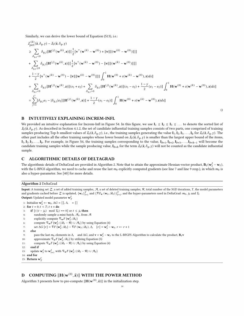
Similarly, we can derive the lower bound of Equation (S13), i.e.:
I (𝑘)pert(z, 𝛿𝑦, 𝛾) − I0 (z, 𝛿𝑦, 𝛾)
≥∑
𝛿𝑦,𝑗<0
𝛿𝑦,𝑗 ∥H( 𝑗) (w(𝑘) , z)∥ [1
2
[v⊤ (w(𝑘) −w(0) ) + ∥v∥∥(w(𝑘) −w(0) )∥]]
+∑
𝛿𝑦,𝑗 ≥0𝛿𝑦,𝑗 ∥H( 𝑗) (w(𝑘) , z)∥ [
1
2
[v⊤ (w(𝑘) −w(0) ) − ∥v∥∥(w(𝑘) −w(0) )∥]]
+ 1 − 𝛾2
[v⊤ (w(𝑘) −w(0) ) − ∥v∥∥w(𝑘) −w(0) ∥]∥∫
1
0
H(w(0) + 𝑠 (w(𝑘) −w(0) ), z)𝑑𝑠 ∥
=∑
𝛿𝑦,𝑗<0
𝛿𝑦,𝑗 ∥H( 𝑗) (w(𝑘) , z)∥(𝑒1 + 𝑒2) +∑
𝛿𝑦,𝑗>0
𝛿𝑦,𝑗 ∥H( 𝑗) (w(𝑘) , z)∥(𝑒1 − 𝑒2) +1 − 𝛾2
(𝑒1 − 𝑒2)∥∫
1
0
H(w(0) + 𝑠 (w(𝑘) −w(0) ), z)𝑑𝑠 ∥
=
𝐶∑𝑗=1
[𝛿𝑦,𝑗𝑒1 − |𝛿𝑦,𝑗 |𝑒2] ∥H( 𝑗) (w(𝑘) , z)∥ +1 − 𝛾2
(𝑒1 − 𝑒2)∥∫
1
0
H(w(0) + 𝑠 (w(𝑘) −w(0) ), z)𝑑𝑠 ∥
□
B INTUITIVELY EXPLAINING INCREM-INFLWe provided an intuitive explanation for Increm-Infl in Figure S4. In this figure, we use I1 ≤ I2 ≤ I3 ≤ . . . to denote the sorted list of
I0 (z, 𝛿𝑦, 𝛾). As described in Section 4.1.2, the set of candidate influential training samples consists of two parts, one comprised of training
samples producing Top-b smallest values of I0 (z, 𝛿𝑦, 𝛾), i.e., the training samples generating the value I1, I2, I3, . . . , I𝑏 for I0 (z, 𝛿𝑦, 𝛾). Theother part includes all the other training samples whose lower bound on I0 (z, 𝛿𝑦, 𝛾) is smaller than the largest upper bound of the items,
I1, I2, I3, . . . , I𝑏 . For example, in Figure S4, the training samples corresponding to the value, I𝑏+1, I𝑏+2, I𝑏+3, . . . , I𝑏+ℎ−1 will become the
candidate training samples while the sample producing value, I𝑏+ℎ for the term I0 (z, 𝛿𝑦, 𝛾) will not be counted as the candidate influential
sample.
C ALGORITHMIC DETAILS OF DELTAGRADThe algorithmic details of DeltaGrad are provided in Algorithm 2. Note that to attain the approximate Hessian-vector product, B𝑡 (w𝐼
𝑡 −w𝑡 ),with the L-BFGS algorithm, we need to cache and reuse the last𝑚0 explicitly computed gradients (see line 7 and line 9 resp.), in which𝑚0 is
also a hyper-parameter. See [40] for more details.
Algorithm 2 DeltaGrad
Input: A training set Z, a set of added training samples, A, a set of deleted training samples, R, total number of the SGD iterations,𝑇 , the model parameters
and gradients cached before Z is updated, {w𝑡 }𝑇𝑡=1 and {∇𝐹w (w𝑡 ,ℬ𝑡 ) }𝑇𝑡=1, and the hyper-parameters used in DeltaGrad:𝑚0, 𝑗0 and𝑇0
Output: Updated model parameter w𝐼𝑇
1: Initialize w𝐼0← w0, Δ𝐺 = [], Δ𝑊 = []
2: for 𝑡 = 0; 𝑡 < 𝑇 ; 𝑡 + + do3: if [ ( (𝑡 − 𝑗0) mod 𝑇0) == 0] or 𝑡 ≤ 𝑗0 then4: randomly sample a mini-batch, A𝑡 , from A5: explicitly compute ∇w𝐹
(w𝐼𝑡 ;ℬ𝑡
)6: compute ∇w𝐹
(w𝐼𝑡 ; (ℬ𝑡 − R) ∪ A𝑡
)by using Equation (4)
7: set Δ𝐺 [𝑟 ] = ∇𝐹(w𝐼𝑡 ;ℬ𝑡
)− ∇𝐹 (w𝑡 ;ℬ𝑡 ) , Δ𝑊 [𝑟 ] = w𝐼
𝑡 −w𝑡 , 𝑟 ← 𝑟 + 18: else9: pass the last𝑚0 elements in Δ𝑊 and Δ𝐺 , and v = w𝐼
𝑡 −w𝑡 to the L-BFGFS Algorithm to calculate the product, B𝑡v10: approximate ∇w𝐹
(w𝐼𝑡 ,ℬ𝑡
)by utilizing Equation (5)
11: compute ∇w𝐹(w𝐼𝑡 ; (ℬ𝑡 − R) ∪ A𝑡
)by using Equation (4)
12: end if13: update w𝐼
𝑡 to w𝐼𝑡+1 with ∇w𝐹
(w𝐼𝑡 ; (ℬ𝑡 − R) ∪ A𝑡
)14: end for15: Return w𝐼
𝑇
D COMPUTING ∥H(w(0) , z)∥WITH THE POWER METHODAlgorithm 3 presents how to pre-compute ∥H(w(0) , z)∥ in the initialization step.
14

Figure S4: Intuitive illustration of Increm-Infl
Algorithm 3 Pre-compute ∥H(w(0) , z)∥ in the initialization step
Input: A training sample z ∈ Z, the class 𝑗 and the model parameter obtained in the initialization step: w(0)
Output: ∥H(w(0) , z) ∥.1: Initialize g as a random vector;
2: ***** Power method below ******
3: while g is not converged do4: Calculate H(w(0) , z)g by using the auto-differentiation package
5: Update g: g =H(w(0) ,z)g∥H(w(0) ,z)g∥
6: end while7: Calculate the largest eigenvalue of H(w(0) , z) in magnitude by using
g⊤H(w(0) ,z)g∥g∥ , which is equivalent to ∥H(w(0) , z) ∥.
8: Return ∥H(w(0) , z) ∥.
Note that the algorithm above relies on the auto-differentiation package for calculating the Hessian-vector product effectively. Specifically,
for a Hessian-vector product H(w(0) , z)g, it can be further rewritten as follows:
H(w(0) , z)g = ∇2w𝐹 (w(0) , z)g = ∇w (∇w𝐹 (w(0) , z))g
= ∇w (∇w𝐹 (w(0) , z)g)(S24)
in which the first equality utilizes the definition of the Hessian matrix while the last equality regards the vector g as a constant with
respect to w and utilizes the chain rule in reverse. Therefore, to obtain the result of H(w(0) , z)g, we can invoke the auto-differentiation
package twice. The first one is on the loss 𝐹 (w(0) , z), resulting in the first order derivative ∇w𝐹 (w(0) , z), while the second one is on the
product ∇w𝐹 (w(0) , z)g, leading to the final result of H(w(0) , z)g.
E TIME COMPLEXITY OF PRIORITIZING THE MOST INFLUENTIAL TRAINING SAMPLES WITHINCREM-INFL
According to Theorem 1, evaluating the bound on I (𝑘)pert(z, 𝛿𝑦, 𝛾) requires four major steps, including 1) computing the Hessian-vector
product, v, by employing the solution shown in Section D, which can be computed once for all training samples (suppose the time complexity
of this step is 𝑂 (𝑣); 2) computing v[∇𝑦∇w𝐹 (w(0) , z)𝛿𝑦 + (1 − 𝛾)∇w𝐹 (w(0) , z)] in I0 (z, 𝛿𝑦, 𝛾) with two matrix-vector multiplications
(recall that ∇𝑦∇w𝐹 (w(0) , z) and ∇w𝐹 (w(0) , z) are pre-computed), which requires 𝑂 (𝐶𝑚) operations (𝑚 is used to denote the dimension of
w); 3) computing v(w(𝑘) −w(0) ) and ∥v∥∥w(𝑘) −w(0) ∥, which requires 𝑂 (𝑚) operations; 4) computing
∑𝐶𝑟=1 |𝛿𝑦,𝑟 |∥H(𝑟 ) (w(𝑘) , z)∥ and∑𝐶
𝑟=1 𝛿𝑦,𝑟 ∥H(𝑟 ) (w(𝑘) , z)∥, which requires 𝑂 (𝐶) operations (recall that ∥H(𝑟 ) (w(𝑘) , z)∥ is also pre-computed). Hence, the overall overhead
of evaluating the bound on I (𝑘)pert(z, 𝛿𝑦, 𝛾) for all 𝑁 training samples and all possible𝐶 classes is𝑂 (𝑣) +𝑁𝐶 (𝑂 (𝐶𝑚) +𝑂 (𝑚) +𝑂 (𝐶)). Suppose
after Algorithm 1 is invoked, 𝑛(≪ 𝑁 ) samples become the candidate influential training samples. Then the next step is to evaluate Equation
(6) on each of those candidate samples for each possible deterministic class. Note that the main overhead of each invocation of Equation
(6) comes from deriving the class-wise gradient ∇𝑦∇w𝐹 (w(𝑘) , z) and the sample-wise gradient ∇w𝐹 (w(𝑘) , z), which is supposed to have
time complexity 𝑂 (Grad). Therefore, the total time complexity of utilizing the Algorithm 1 first and evaluating Equation (6) on 𝑛 candidate
training samples afterwards is 𝑂 (𝑣) + 𝑁𝐶 (𝑂 (𝐶𝑚) +𝑂 (𝑚) +𝑂 (𝐶)) + 𝑛𝑐𝑂 (Grad). In contrast, without utilizing Algorithm 1, it is essential to
evaluate Equation (6) on every training sample which thus requires 𝑂 (𝑣) + 𝑁𝐶 ·𝑂 (Grad) operations. Considering the fact that the time
overhead of single gradient computation is much larger than 𝑂 (𝐶𝑚), 𝑂 (𝑚) or 𝑂 (𝐶), then we can expect that with small 𝑛, Increm-Infl can
lead to significant speed-ups.
15

F SUPPLEMENTARY EXPERIMENTAL SETUPSF.1 Details of the datasetsMIMIC dataset is a large chest radiograph dataset containing 377,110 images, which have been partitioned into training set, validation set
and test set. There are 13 binary labels for each image, corresponding to the existence of 13 different findings. Those labels are automatically
extracted from the text [19], thus leading to possibly undetermined labels for some finds. In the experiments, we focused on predicting
whether the finding “Lung Opacity” exists for each image and only retained those training samples with determined binary labels for this
finding, eventually producing 85046 samples, 579 samples and 1628 samples in the training set, validation set and test set respectively.
Chexpert dataset is another large chest radiograph dataset consisting of 223,415 X-ray images as the training set and another 234
images as the validation set. Since the test set is not publicly available yet, we regard the original validation set as the test set and randomly
selected 10% of the training samples as the validation set. This dataset is used to predict whether each of the 14 observations exists in each
X-ray image. In the experiments, we focus on predicting the existence of the observation “Cardiomegaly” in each image. Similar to the
pre-processing operations on MIMIC, we removed the training samples and the validation samples with undetermined labels (labeled as -1)
for this observation, leading to 38629 samples and 4251 samples in the training set and validation set respectively. All the test samples, i.e.
the original validation samples, are fully labeled, which are all retained in the experiments.
Retina dataset is an image dataset consisting of fully labeled retinal fundus photographs [12]. The target use of this dataset is to diagnose
one eye disease called Diabetic Retinopathy (DR) for each image, which is classified into 5 categories based on severity. We followed [32] to
predict whether an image belongs to a referable DR, which regard the label 1 and 2 as the referable one and the label 3-5 as the non-referable
one. As a consequence, the original five-class classification problem is transformed into a binary classification problem. In the original
version of Retina dataset, there are 35127 samples and 53576 samples in the training set and test. We randomly select 10% of the training
samples as the validation samples and use the rest of them as the training set in the experiments.
Fashion dataset includes 30525 images and the label of each image represents whether it is fashionable or not, annotated by three
different human annotators. In addition to those labels, some text information such as the users’ comments is also associated with each
image. However, ground-truth labels are not available in this dataset and simulated with the labels by aggregating the human annotated
labels through majority vote. For the experiments in Section 5, similar to Fully clean datasets, we apply ResNet50 for feature transformation
and run logistic regression model afterwards.
Fact dataset Each sample in Fact dataset is an RDF triple for representing one fact and there are over 40000 of such facts. Each such fact
is labeled as true, false or ambiguous by five different human annotators. But the total number of human annotators is 57. Among all the
samples, only 577 samples have ground-truth labels. In the experiments, we removed the samples with the ground-truth label “ambiguous”
and randomly partition the remaining samples with ground-truth labels into two parts, Although there are three different labels, we ignore
the label ‘ambiguous’, meaning that we only conduct a binary classification task on this dataset. However, it is likely that the aggregated label
for some uncleaned training sample becomes ‘ambiguous’ even after we resolve the labeling conflicts between different human annotators.
To deal with this, the probabilistic labels of this sample is not updated for representing the labeling uncertainties from the human annotators.
To facilitate the feature transformation as mentioned in Section 5, we concatenate each RDF triple as one sentence and then employ the
pre-trained bert-based transformer [8] for transforming each raw text sample into a sequence of embedding vectors. To guarantee batch
training on this dataset, only the last 20 embedding vectors are used. If the total number of embedding sequence for a sample is smaller than
20, we pad this sequence with zero vectors. As introduced in Section 5, to identify whether a fact is true or not, it is essential to compare this
RDF triple against the associated evidence (represented by a sentence). Therefore, by following the above principle, we transform each piece
of evidence into a embedding sequence and trim the length of this sequence to 20 for accelerating the training process.
Twitter dataset is comprised of ∼12k tweets for sentimental analysis. In other words, the classification problem on this dataset is to
judge whether the expression in each tweet is positive, negative or neutral. The labels of those samples are provided by a group of 507 human
annotators and each individual tweet is labeled by three different human annotators. Among all the samples, 577 of them have ground-truth
labels. Similar to Fact dataset, only the positive label and the negative label are employed in the experiments. Therefore, the samples taking
the neutral label as the ground truth are removed. Also, if the aggregated human annotated labels on one uncleaned sample is neural, then
the probabilistic label on this sample is not updated Plus, we generate a 768-D embedding sequence by running the pre-trained bert-based
transformer on each tweet and trim the length of the resulting embedding sequence to 20. When logistic regression model is used,
The detailed statistics of the above six datasets are included in Table 3.
Table 3: Sizes of Fully clean datasets and Crowdsourced datasets
Dataset MIMIC Retina Chexpert Fashion Fact Twitter
Training set 78487 31615 37882 29031 38176 11606
Validation set 579 3512 234 146 255 37
Test set 1628 53576 234 146 259 37
# of samples with ground
truth
80649 88703 43114 29323 514 74
16

F.2 Hyper-parameters for model trainingWe included all the other hyper-parameters in Table 4, which are determined through grid search. In addition, notice that applying DeltaGrad
or Retrain to update the model parameters may lead to the termination of the training process at different epochs. Therefore, for fair
comparison of the running time for DeltaGrad and Retrain, we run SGD for fixed number of epochs and record the running time of the two
methods. After the training process is done. we apply the early stopping on the model parameters cached at each SGD epoch to determine
the model parameters.
Recall that for DeltaGrad, to balance between the approximation error and efficiency in DeltaGrad, ∇w𝐹 (w𝐼𝑡 ,ℬ𝑡 ) is explicitly evaluated in
the first 𝑗0 SGD iterations and every 𝑇0 SGD iterations afterwards, where 𝑇0 and 𝑗0 are pre-specified hyper-parameters. Also, As Algorithm
2 indicates, the use of L-BFGS algorithm also requires last𝑚0 explicitly evaluated gradients and model parameters as the input. In the
experiments, we set up the above three hyper-parameters as,𝑚 = 2, 𝑗0 = 10 and 𝑇0 = 10 for all six datasets.
Table 4: The hyper-parameters for each dataset
Dataset MIMIC Retina Chexpert Fashion Fact Twitter
Learning rate 0.0005 0.001 0.02 0.05 0.005 0.01
L2 regularization 0.05 0.05 0.05 0.001 0.01 0.01
# of epochs 150 200 200 200 150 400
F.3 Adapting DUTI to handle probabilistic labelsAccording to [42], the original version of DUTI is as follows:
min
Y′=[𝑦′1,𝑦′
2,...,𝑦′𝑛 ],w
[ 1
|Zval|
∑z∈Zval
𝐹 (w, z) + 1
𝑛
𝑛∑𝑖=1
𝐹 (w, (x, 𝑦′𝑖 )) +𝛾
𝑛
𝑛∑𝑖=1
(1 − 𝑦′𝑖,𝑦𝑖 )],
s.t. w = argminw1
𝑛
𝑛∑𝑖=1
𝐹 (w, (x𝑖 , 𝑦′𝑖 ))(S25)
which is defined on the training datasetZ = {(x𝑖 , 𝑦𝑖 )}𝑛𝑖=1 and the validation datasetZval
= {(x𝑖 , 𝑦𝑖 )} |Zval |𝑖=1
. In the formula above, each 𝑦′𝑖
is a vector of length 𝐶 (recall that 𝐶 represents the number of classes) and the term 𝑦′𝑖,𝑦𝑖
indicates the (𝑦𝑖 )𝑡ℎ entry in the vector 𝑦′𝑖, which
implicitly suggests that each 𝑦𝑖 should be a deterministic label.
Note that if 𝑦𝑖 is a probabilistic label (represented by a probabilistic vector of length 𝐶), we cannot calculate the term 𝑦′𝑖,𝑦𝑖
. Therefore, we
replace 𝑦𝑖 in 𝑦′𝑖,𝑦𝑖
by using the index with the largest entry in 𝑦𝑖 .
G SUPPLEMENTARY EXPERIMENTSG.1 Detailed experimental results of Exp1The detailed experimental results of Exp1 are included in Table 5 and Table 6 respectively for 𝑏 = 100 and 𝑏 = 10.
Table 5: Comparison of the model prediction performance (F1 score) after 100 training samples are cleaned (𝑏 = 100, 𝛾 = 0.8)
uncleaned Infl-D Active (one) Active (two) O2U Infl (one) Infl (two) Infl (three)
MIMIC 0.6284±0.0012 0.6283±0.0011 0.6286±0.0008 0.6286±0.0008 0.1850±0.0006 0.6292±0.0005 0.6293±0.0012 0.6293±0.0008Retina 0.5565±0.0019 0.5556±0.0012 0.5566±0.0029 0.5566±0.0029 0.1331±0.0012 0.5580±0.0013 0.5582±0.0011 0.5581±0.0009Chexpert 0.5244±0.0016 0.5244±0.0033 0.5248±0.0024 0.5248±0.0024 0.5276±0.0012 0.5286±0.0023 0.5297±0.0022 0.5289±0.0022Fashion 0.5140±0.0142 0.5143±0.0146 0.5145±0.0144 0.5145±0.0144 0.5148±0.0142 0.5178±0.0132 0.5177±0.0132 0.5177±0.0126Fact 0.6595±0.0017 0.6596±0.0018 0.6598±0.0017 0.6598±0.0017 0.6599±0.0014 0.6601±0.0021 0.6609±0.0021 0.6603±0.0021Twitter 0.6485±0.0050 0.6530±0.0088 0.6540±0.0045 0.6540±0.0045 0.6481±0.0023 0.6594±0.0034 0.6680±0.0044 0.6594±0.0032
Table 6: Comparison of the model prediction performance (F1 score) after 100 training samples are cleaned (𝑏 = 10, 𝛾 = 0.8)
uncleaned Infl-D Active (one) Active (two) O2U Infl (one) Infl (two) Infl (three)
MIMIC 0.6284±0.0012 0.6283±0.0011 0.6287±0.0005 0.6287±0.0005 0.1850±0.0008 0.6292±0.0007 0.6293±0.0011 0.6292±0.0008Retina 0.5565±0.0019 0.5556±0.0016 0.5568±0.0001 0.5568±0.0016 0.1314±0.0006 0.5579±0.0013 0.5582±0.0003 0.5581±0.0018
Chexpert 0.5244±0.0016 0.5246±0.0036 0.5246±0.0020 0.5246±0.0020 0.5281±0.0016 0.5287±0.0024 0.5300±0.0024 0.5291±0.0023Fashion 0.5140±0.0142 0.5143±0.0144 0.5145±0.0135 0.5145±0.0135 0.5152±0.0143 0.5178±0.0125 0.5181±0.0131 0.5180±0.0128Fact 0.6595±0.0017 0.6596±0.0018 0.6600±0.0017 0.6600±0.0017 0.6598±0.0010 0.6601±0.0019 0.6609±0.0020 0.6602±0.0022
Twitter 0.6485±0.0050 0.6518±0.0081 0.6515±0.0082 0.6515±0.0082 0.6490±0.0067 0.6578±0.0039 0.6697±0.0058 0.6586±0.0032
17

Table 7: Comparison of the model prediction performance (F1 score) after 100 training samples are cleaned (CNN)
b=100 b=10
uncleaned Infl
(one)
Infl
(two)
Infl
(three)
Infl
(one)
Infl
(two)
Infl
(three)
Infl-D Active
(one)
Active
(two)
O2U
MIMIC 0.8897 0.8895 0.8883 0.8893 0.8893 0.8908 0.8904 0.8895 0.8895 0.8895 0.8873
Retina 0.5529 0.5577 0.5636 0.5602 0.5596 0.5645 0.5607 0.5556 0.5574 0.5574 0.5608
Fact 0.7510 0.7536 0.8027 0.7636 0.7553 0.8063 0.7654 0.7560 0.7566 0.7516 0.7739
Twitter 0.6609 0.6727 0.6828 0.6783 0.6585 0.6907 0.6745 0.6642 0.6544 0.6610 0.6740
Table 8: Comparison of the model prediction performance (F1 score) after 100 training samples are cleaned (against TARS,b=100)
uncleaned Infl-D Active (one) Active (two) O2U TARS Infl (one) Infl (two) Infl (three)
MIMIC 0.6413±0.0008 0.6647±0.0129 0.6569±0.0240 0.6569±0.0240 0.6686±0.0016 0.6022±0.0016 0.6606±0.0117 0.6375±0.0445 0.6600±0.0079Chexpert 0.5359±0.0040 0.5506±0.0015 0.5404±0.0025 0.5404±0.0025 0.5419±0.0008 0.5257±0.0031 0.5505±0.0022 0.5671±0.0065 0.5537±0.0037Retina 0.5702±0.0015 0.6077±0.0090 0.5910±0.0028 0.5910±0.0028 0.6021±0.0110 0.5573±0.0295 0.6015±0.0082 0.6168±0.0063 0.6057±0.0076Fashion 0.6280±0.0035 0.6318±0.0047 0.6329±0.0070 0.6329±0.0070 0.6380±0.0027 0.4964±0.0022 0.6365±0.0022 0.6460±0.0060 0.6372±0.0026
Table 9: Comparison of the model prediction performance (F1 score) after 100 training samples are cleaned (against TARS,b=10)
uncleaned Infl-D Active (one) Active (two) O2U TARS Infl (one) Infl (two) Infl (three)
MIMIC 0.6413±0.0008 0.6874±0.0110 0.6815±0.0063 0.6815±0.0063 0.6698±0.0019 0.6025±0.0008 0.6867±0.0005 0.6968±0.0220 0.6925±0.0149Chexpert 0.5359±0.0040 0.5581±0.0119 0.5404±0.0136 0.5404±0.0136 0.5396±0.0045 0.5333±0.0029 0.5626±0.0061 0.5863±0.0046 0.5579±0.0128Retina 0.5702±0.0015 0.6098±0.0111 0.5989±0.0062 0.5989±0.0062 0.6026±0.0012 0.5572±0.0296 0.6136±0.0097 0.6347±0.0034 0.6173±0.0070Fashion 0.6280±0.0035 0.6318±0.0047 0.6329±0.0070 0.6329±0.0070 0.6380±0.0027 0.4964±0.0022 0.6365±0.0022 0.6460±0.0060 0.6372±0.0026
G.2 Comparing Infl against baseline methods with neural network modelsIn this section, we conduct some initial experiments when neural network models are used in theModel constructor. To goal is to compare Infl
(with different strategies to clean labels) against all the baseline methods mentioned in Section 5 (including Infl-D, Active (one), Active (two),
and O2U) in this more general setting. Specifically, for the image dataset, we applied the LeNet [22] (a classical type of convolutional neural
network structure) on the original image features (instead of features transformed by using transfer learning). For the text dataset, such as Fact
and Twitter dataset, similar to Section 5, we still transform each plain-text sample into the corresponding embedding representations by using
the pre-trained bert-based transformer and then applied one 1D convolutional neural network on the resulting embedding representations.
We found that the performance of applying LeNet model on Fashion and Chexpert dataset is significantly worse than that when the
pre-trained models are used, even when all the probabilistic labels are replaced with the ground-truth labels or the aggregated human
annotated labels. Therefore, we only present the experimental results on MIMIC, Retina, Fact and Twitter dataset, which are included in
Table 7.
As Table 7 indicates, Infl (two) can still achieve the best model performance for those four datasets, thus indicating the potential of
applying Infl even when neural network model is used. Note that LeNet model is obviously less complicated than other large neural network
models, such as ResNet50. Therefore, in the future, we would do more extensive experiments to evaluate the performance of Infl when
those large neural network models are used. In addition, recall that unlike Infl, Increm-Infl and DeltaGrad-L are only applicable for strongly
convex models such as logistic regression models. How to extend those two methods to handle neural network models will also be part of
the future work.
G.3 Comparing Infl against TARSAs claimed in Section 5, similar to Infl, TARS [9] also targets prioritizing the most influential uncleaned training samples for cleaning.
However, this method explicitly assumes that all the labels (no matter they are clean or not) are either 0 or 1 rather than probabilistic labels,
thus indicating its inapplicability in the presence of the probabilistic labels. To facilitate a fair comparison between Infl and TARS, we round
the probabilistic labels on the uncleaned training samples to the nearest deterministic labels and still regularize those samples.
In addition, we notice that to determine the influence of each uncleaned training sample, TARS needs to estimate how each uncleaned
label will be changed if it is to be cleaned. This depends on “all” the possible combinations of labels provided by “all” human annotators,
which are thus exponential in the number of human annotators. Therefore, since the number of human annotators for Fact and Twitter
dataset is not small (over 50), we only compare Infl against TARS on Fully clean datasets and Fashion dataset. In this experiment, we still
train logistic regression models on the features transformed by using the pre-trained models and use the same hyper-parameters as Section
5. In the end, we summarize the experimental results in Table 8-9.
18

Table 10: Comparison of the model prediction performance (F1 score) after 100 training samples are cleaned (𝑏 = 100, 𝛾 = 1)
uncleaned Infl-D Infl-Y DUTI Active
(one)
Active
(two)
O2U Infl (one) Infl (two) Infl (three)
MIMIC 0.6310±0.0010 0.6310±0.0010 0.6310±0.0011 0.6310±0.0011 0.6314±0.0008 0.6314±0.0008 0.1278±0.0080 0.6320±0.0011 0.6321±0.0011 0.6321±0.0010Retina 0.5547±0.0020 0.5543±0.0015 0.5546±0.0019 0.5558±0.0019 0.5554±0.0018 0.5554±0.0018 0.0940±0.0023 0.5564±0.0020 0.5567±0.0021 0.5565±0.0021Chexpert 0.5360±0.0123 0.5354±0.0108 0.5360±0.0118 0.5361±0.0127 0.5366±0.0127 0.5366±0.0127 0.5282±0.0043 0.5403±0.0122 0.5444±0.0080 0.5403±0.0131Fashion 0.5264±0.0078 0.5262±0.0076 0.5265±0.0081 0.5238±0.0070 0.5267±0.0041 0.5267±0.0041 0.5277±0.0065 0.5297±0.0068 0.5301±0.0053 0.5299±0.0059Fact 0.6584±0.0015 0.6587±0.0016 0.6584±0.0015 0.6582±0.0056 0.6580±0.0020 0.6580±0.0020 0.6587±0.0006 0.6586±0.0016 0.6588±0.0016 0.6585±0.0017Twitter 0.7034±0.0062 0.6853±0.0140 0.7102±0.0125 0.6230±0.0149 0.7051±0.0089 0.7051±0.0089 0.6401±0.0175 0.7164±0.0017 0.7349±0.0290 0.7200±0.0109
Table 11: Comparison of the model prediction performance (F1 score) after 100 training samples are cleaned (𝑏 = 10, 𝛾 = 1)
uncleaned Infl-D Infl-Y Active (one) Active (two) O2U Infl (one) Infl (two) Infl (three)
MIMIC 0.6310±0.0010 0.6310±0.0010 0.6310±0.0011 0.6316±0.0007 0.6316±0.0007 0.1284±0.0077 0.6321±0.0010 0.6321±0.0010 0.6321±0.0010Retina 0.5547±0.0020 0.5543±0.0015 0.5547±0.0018 0.5552±0.0018 0.5552±0.0018 0.0934±0.0021 0.5564±0.0018 0.5567±0.0019 0.5564±0.0019Chexpert 0.5360±0.0123 0.5355±0.0112 0.5359±0.0121 0.5368±0.0127 0.5368±0.0127 0.5281±0.0036 0.5402±0.0117 0.5412±0.0120 0.5406±0.0124Fashion 0.5264±0.0078 0.5263±0.0076 0.5265±0.0081 0.5268±0.0041 0.5268±0.0041 0.5275±0.0065 0.5298±0.0068 0.5303±0.0053 0.5300±0.0059Fact 0.6584±0.0015 0.6585±0.0015 0.6585±0.0017 0.6584±0.0021 0.6584±0.0021 0.6586±0.0020 0.6585±0.0016 0.6588±0.0016 0.6585±0.0017Twitter 0.7034±0.0062 0.5854±0.0099 0.6999±0.0020 0.7030±0.0109 0.7030±0.0109 0.6268±0.0069 0.7153±0.0019 0.7420±0.0019 0.7171±0.0029
Table 12: Comparison of the model prediction performance (F1 score) after 100 training samples are cleaned (𝑏 = 100, 𝛾 = 0)
uncleaned Infl-D Active (one) Active (two) O2U Infl (one) Infl (two) Infl (three)
MIMIC 0.6323±0.0041 0.8880±0.0174 0.8641±0.0348 0.8641±0.0348 0.8933±0.0082 0.8740±0.0306 0.8989±0.0008 0.8853±0.0196Retina 0.5614±0.0018 0.6728±0.0138 0.6898±0.0038 0.6898±0.0038 0.6707±0.0340 0.6756±0.0133 0.6894±0.0048 0.6884±0.0077Chexpert 0.5231±0.0009 0.5709±0.0059 0.5752±0.0512 0.5752±0.0512 0.5825±0.0195 0.5853±0.0238 0.5924±0.0171 0.5878±0.0188Fashion 0.5057±0.0163 0.5789±0.0437 0.5593±0.0089 0.5593±0.0089 0.5830±0.0021 0.5905±0.0212 0.6020±0.0431 0.5975±0.0139Fact 0.6604±0.0020 0.6584±0.0221 0.6723±0.0185 0.6723±0.0185 0.6553±0.0232 0.6618±0.0192 0.6691±0.0159 0.6616±0.0221Twitter 0.6335±0.0301 0.6534±0.0248 0.6324±0.0024 0.6324±0.0112 0.7703±0.0210 0.6029±0.0689 0.6739±0.0403 0.6232±0.0560
According to Table 8-9, Infl still results in much better models than other baseline methods, including TARS. This thus demonstrates the
performance advantage of Infl even when the uncleaned labels are all deterministic. So in comparison to TARS, Infl is not only suitable for
more general scenarios, but also capable of producing higher-quality models in those scenarios.
G.4 Vary the weight for the uncleaned training samplesWe also repeat the Exp1 in Section 5 with varied weights on the uncleaned training samples, i.e. varied 𝛾 in Equation (1). Specifically, we use
two different 𝛾 ′s, 1 and 0. The results with 𝛾 = 0 and 𝛾 = 1 are included in Table 10-11 and Table 12-13 respectively.
First of all, when 𝛾 = 1, we can observe that either Infl (one) or Infl (two) or Infl (three) achieves the best model performance. Since both
Infl (two) and Infl (three) involve the labels suggested by Infl, it therefore again indicates those labels are reasonable.
It is also worth noting that when 𝛾 is one where all the training samples are equally weighted. DUTI performs worse than Infl. Based on
our observations in the experiments, this phenomenon might be due to the difficulty in exactly solving the bi-optimization problem in DUTI,
thus producing sub-optimal selections of the influential training samples.
Plus, when 𝛾 = 1, we also observe that Infl-Y performs worse than Infl. Recall that by comparing against Infl, Infl-Y quantifies the influence
of each training sample without taking the magnitude of the label changes into the considerations. Since Infl-Y fails to outperform Infl, it
thus justifies the necessity of explicitly considering the label changes in the influence function.
On the other hand, when 𝛾 = 0, except MIMIC and Retina, Infl can still beat other baseline methods, thus indicating that the potential of
Infl when the uncleaned labels are not included in the training process. Note that for MIMIC and Retina dataset, the performance of Infl is
not ideal. One possible reason is that with 𝛾 = 0, the samples with probabilistic labels are not included in the training process, meaning that
only a small portion of samples (up to 100) are used for model training. Note that there are 100 samples cleaned in total, thus violating the
small cleaning budge assumption. Plus, note that for the influence function method, due to the Taylor expansion in Equation (S11), one
implicit assumption is thus the slight modification on model parameter after small amount of training samples are modified. However, we
also observe that significant updates on the model parameters occur after the 100 samples are cleaned for MIMIC and Retina dataset (due to
the violation of the small cleaning budge assumption), thus leading to inaccurate estimate on the training sample influence. How to handle
this pathological scenario will be also part of our future work.
Lastly, by comparing Table 10-11 and Table 12-13, it is worth noting that with 𝛾 = 1, the model performance is worse with respect to that
with 𝛾 = 0, thus implying the negative effect of the probabilistic labels. But as we can see, when 𝛾 = 1, the strong negative effect of the
probabilistic labels do not hurt the performance of Infl, thus suggesting the robustness of Infl when the probabilistic labels are not ideal.
19

Table 13: Comparison of the model prediction performance (F1 score) after 100 training samples are cleaned (𝑏 = 10, 𝛾 = 0)
uncleaned Infl-D Active (one) Active (two) O2U Infl (one) Infl (two) Infl (three)
MIMIC 0.6323±0.0041 0.9013±0.0006 0.9008±0.0007 0.9007±0.0007 0.9010±0.0008 0.9007±0.0004 0.8991±0.0012 0.9008±0.0010Retina 0.5614±0.0018 0.6550±0.0613 0.6916±0.0038 0.6916±0.0038 0.6962±0.0193 0.6902±0.0007 0.6904±0.0254 0.6802±0.0108Chexpert 0.5231±0.0009 0.5736±0.0100 0.5890±0.0190 0.5890±0.0190 0.5775±0.0271 0.6275±0.0329 0.6382±0.0225 0.6254±0.0206Fashion 0.5057±0.0163 0.5956±0.0296 0.5651±0.0407 0.5651±0.0407 0.5498±0.0486 0.6449±0.0126 0.6926±0.0148 0.6706±0.0174Fact 0.6604±0.0020 0.6511±0.0306 0.6532±0.0305 0.6532±0.0305 0.6829±0.0157 0.6576±0.0283 0.6871±0.0801 0.6582±0.0229Twitter 0.6335±0.0301 0.6140±0.0226 0.6891±0.0024 0.6891±0.0086 0.7547±0.0087 0.7406±0.1798 0.8184±0.0446 0.7711±0.0258
Table 14: Comparison of the model prediction performance (F1 score) with varied 𝑏 on Twitter dataset (Infl (two))
uncleaned b=1000 b=500 b=200 b=100 b=50 b=20 b=10
Twitter 0.6509 0.8672 0.8932 0.8939 0.9149 0.9105 0.9046 0.9064
Fashion 0.6605 0.6942 0.6993 0.6990 0.7042 0.7065 0.7089 0.7082
G.5 Vary the size of 𝑏As the first step toward determining an appropriate 𝑏 to balance the model performance and the running time given a fixed cleaning
budget, we set up the clean budget as 1000 and vary 𝑏 from 10 to 1000. All the other hyper-parameters are the same as that in Section
5. The experimental results are provided in Table 14. As this table shows, roughly speaking, when the cleaning budget is 1000 and 𝑏 is
100, i.e. roughly 10% of the cleaning budget, the model performance is close to the peak performance. After 𝑏 becomes even smaller, the
model performance will not be significantly improved but will increase the overall running time. Therefore, to balance between the model
performance and the running time, setting 𝑏 as the 10% of the cleaning budget would be recommended.
20
Related Documents