Chebyshev polynomials and Fourier transform of SU (2) irreducible representation character as spin tomographic star-product kernel

arX

iv:0

905.

4944

v1 [

quan

t-ph

] 2

9 M

ay 2

009

Chebyshev polynomials and Fourier transform

of SU(2) irreducible representation character

as spin-tomographic star-product kernel

S. N. Filippov1∗ and V. I. Man’ko2†

1Moscow Institute of Physics and Technology (State University)

Institutskii per. 9, Dolgoprudnyi, Moscow Region 141700, Russia2P. N. Lebedev Physical Institute, Russian Academy of Sciences

Leninskii Prospect 53, Moscow 119991, Russia

Spin-tomographic symbols of qudit states and spin observables are studied. Spin

observables are associated with the functions on a manifold whose points are labelled

by spin projections and sphere S2 coordinates. The star-product kernel for such func-

tions is obtained in explicit form and connected with Fourier transform of characters

of SU(2) irreducible representation. The kernels are shown to be in close relation

to the Chebyshev polynomials. Using specific properties of these polynomials, we

establish the recurrence relation between kernels for different spins. Employing the

explicit form of the star-product kernel, a sum rule for Clebsch-Gordan and Racah

coefficients is derived. Explicit formulas are obtained for the dual tomographic star-

product kernel as well as for intertwining kernels which relate spin-tomographic

symbols and dual tomographic symbols.

Keywords: spin tomography, star-product, kernel, quantizer, dequantizer, SU(2)-group char-

acter, qudit

I. INTRODUCTION

In quantum mechanics, states of a system are usually associated with the density op-erators. The other possibility is to use different maps of quantum states onto the quasi-probability functions [1, 2] or the fair probability-distribution function called tomogram(see, e.g., [3, 4, 5, 6, 7, 8, 9]). The latter one is of great interest because it can be measuredexperimentally [10, 11, 12, 13, 14]. Though tomograms are often utilized with the onlyaim to reconstruct the Wigner function or the density matrix, it should be emphasized thattomograms themselves are a primary notion of quantum states. As far as spin states areconcerned, the corresponding tomographic map is elaborated in [15, 16, 17, 18, 19]. Theexamples of other maps of spin states onto functions are discussed in [20, 21, 22]. By analogywith the density operator, any other operator (observable) on a Hilbert space can be mappedonto the function called tomographic symbol of the operator. Such a scanning procedure isacomplished with the help of the special dequantizer operator [9, 23]. Using the quantizeroperator [9, 23], one can reconstruct the operator in question, i.e, there exists an inversemap of tomographic symbols onto operators. Within the framework of the spin-tomographic

∗Electronic address: [email protected]†Electronic address: [email protected]

2

star-product procedure [24, 25, 26], one deals with symbols instead of operators. In partic-ular, the symbol of the product of two operators is equal to the star-product of the symbolscorresponding to the separate operators. The main feature of the star-product is that it isassociative but noncommutative in general. The star-product kernel is easily expressed interms of the dequantizer and quantizer operators. The explicit formula of the kernel waspresented previously with the help of Clebsch-Gordan and Racah coefficients in the work[27] and specified for the low-spin states in [28].

The aim of this work is to obtain a new explicit formula of the spin-tomographic star-product kernel in terms of SU(2) irreducible representation character. As mentioned above,any qudit state can be described by the spin-tomographic probability introduced in [15, 16],where the reconstructed states are expressed in terms of such state characteristics as theWigner function or the density matrix. In the work [29], the discussion is presented howto use such a tomographic probability-distribution in the other known reconstruction pro-cedure. Both the spin tomogram, which coincides with that introduced in [15, 16], andthe inversion formula, which provides the density operator of a spin state by means of itsspin tomogram, were given in [29] in the compact exponential forms. On the other hand, itwas proved in [28] that the exponential form of the inversion formula, the inversion formulafound in [16], and that presented in another form in [27] are all identical on the set of spintomograms. In view of this equivalency, one can use any form of the inversion formula onan equal footing. This means that any form of the quantizer and dequantizer operators isacceptable to study concrete properties of the star-product representation of spin operatorsand qudit states. In the present paper, the problem is attacked with the help of exponentialrepresentation of the quantizer and dequantizer operators. The SU(2) irreducible represen-tation character is known to be nothing else but the Chebyshev polynomial of a specificargument. In turn, the kernel is shown to be a Fourier transformation of the character. Weexploit special properties of the Chebyshev polynomials not only to derive the star-productkernel but also to reveal its peculiarities, for instance, the recurrence relation. Comparingdifferent explicit forms of the star-product kernels, we show that the kernel is not definedunambiguously, but the residual must give zero while integrating with tomographic symbols.We point out that the constructed kernels of the spin-tomographic star-product are givenfor the functions which depend not only on group element of SU(2) but also on weights(spin projection m) of SU(2) irreps.

The paper is organized as follows.In Sec. II, we give a brief review of the scanning and reconstruction procedures which

are performed in the spin tomography of qudit states. In Sec. III, the star-product kernelis represented in the form of Fourier transformation of the SU(2) irreps character and theexplicit formula for the kernel is derived. In Sec. IV, we compare two different explicit formsof the kernel to obtain a new sum rule for Clebsch-Gordan and Racah coefficients. In Sec.V, we establish the recurrence relation between the star-product kernels for different spins.In Sec. VI, conclusions are presented. The ambiguity of the spin-tomographic star-productkernel is illustrated in Appendix A. Generalization of the explicit formulas to other typesof kernels is given in Appendix B.

3

II. SPIN TOMOGRAMS AND TOMOGRAPHIC SYMBOLS OF OPERATORS

Unless specifically stated, qudit states with spin j are considered. We deal with theangular momentum operators Jx, Jy, and Jz and the standard state vectors |jm〉 defined asfollows:

(J2x + J2

y + J2z )|jm〉 = j(j + 1)|jm〉, Jz|jm〉 = m|jm〉, (1)

with the spin projection m taking the values −j,−j + 1, . . . , j.As stated above, the state of a qudit is completely determined by its density operator ρ

or alternatively by the following probability-distribution function (called spin tomogram):

wj(m,n) = 〈jm|R†(n)ρR(n)|jm〉 = Tr(

ρ R(n)|jm〉〈jm|R†(n))

= Tr(

ρUj(m,n))

, (2)

where we introduced the dequantizer operator U(m,n) and the rotation operator R(n). Thevector n(θ, φ) = (cos φ sin θ, sin φ sin θ, cos θ) determines the axis of quantization (the pointon the sphere specified by the longitude φ ∈ [0, 2π] and the latitude θ ∈ [0, π]). The rotationoperator is defined through

R(n) = e−i(n⊥· J)θ, n⊥ = (− sin φ, cosφ, 0). (3)

The tomogram satisfies the following normalization conditions:

j∑

m=−j

wj(m,n) = 1,2j + 1

4π

2π∫

0

dφ

π∫

0

sin θdθ wj(m,n(θ, φ)) = 1. (4)

Some other features of the spin-tomographic functions are discussed in [30, 31, 32, 33].

Taking into account the relation R(n)JzR†(n) = (n · J) ≡ nαJα, the dequantizer operator

Uj(m,n) can be written in the following exponential form:

Uj(m,n) = R(n)|jm〉〈jm|R†(n) = R(n)δ(m − Jz)R†(n) = δ

(

m − R(n)JzR†(n)

)

= δ(

m − (n · J))

=1

2π

2π∫

0

eimϕe−i(n·J)ϕdϕ, (5)

where by δ we denote the Kronecker delta-symbol [34].Given the tomogram (2), one can reconstruct the density operator ρ with the help of the

quantizer operator Dj(m,n). The reconstruction procedure reads

ρ =

j∑

m=−j

1

4π

2π∫

0

dφ

π∫

0

sin θdθ wj(m,n(θ, φ))Dj(m,n(θ, φ)) (6)

or briefly

ρ =

∫

wj(x)Dj(x)dx, (7)

4

where we denoted

x = (m,n),

∫

dx =

j∑

m=−j

1

4π

∫

dΩ =

j∑

m=−j

1

4π

2π∫

0

dφ

π∫

0

sin θdθ. (8)

Similarly to the case of dequantizer, the quantizer operator Dj(x) can be represented inthe exponential form [29]

Dj(m,n) =2j + 1

π

2π∫

0

sin2(ϕ/2)eimϕe−(n·J)ϕdϕ =2j + 1

2π

1∑

s=−1

1

1 − 3s2

2π∫

0

ei(m+s)ϕe−i(n·J)ϕdϕ.

(9)Both quantizer and dequantizer are Hermitian operators, with the latter one being non-

negative as well.By analogy with the density operator, any spin operator A acting on a Hilbert space of

states (1) is mapped onto the function fA(x) and vice versa. By construction, the relation

between the tomographic symbol fA(x) and the operator A reads

fA(x) = Tr(

AUj(x))

, A =

∫

fA(x)Dj(x)dx. (10)

Besides usual tomographic symbols described above, sometimes it is convenient to usedual tomographic symbols defined through

fdA(x) = Tr

(

ADj(x))

, A =

∫

fdA(x)Uj(x)dx. (11)

For instance, the average value of the operator A reads

Tr(

ρA)

= Tr

∫

wj(x)Dj(x)A dx =

∫

wj(x)Tr(

ADj(x))

dx =

∫

wj(x)fdA(x)dx. (12)

This implies that one can calculate mean values of observables by using standard and dualtomographic symbols only. The dual tomographic symbols were anticipated in the work [8]and elaborated in [23, 35]. Quantumness of qudit states was demonstrated by means of dualtomographic symbols in [36].

III. KERNEL OF STAR-PRODUCT FOR SPIN TOMOGRAPHIC SYMBOLS

Since operators and tomographic symbols are in strong relation with each other, anyoperation on A and B corresponds to an adequate operation on functions fA(x) and fB(x).

For instance, the sum of A and B maps to the sum of fA(x) and fB(x). As far as the product

AB is concerned, the corresponding tomographic symbol fAB(x) is called the star-productof the symbols fA(x) and fB(x):

fAB(x) = fA(x) ⋆ fB(x). (13)

5

By definition, one has

fAB(x1) = Tr(

ABUj(x1))

=

∫∫

fA(x3)fB(x2)Kj(x3,x2,x1)dx2dx3, (14)

where the function

Kj(x3,x2,x1) = Tr(

Dj(x3)Dj(x2)Uj(x1))

(15)

is called the kernel of the star-product scheme. It is worth noting that this kernel is non-local.The non-locality of kernels of this type can also be illustrated if we consider delta-functionon the tomogram set. In fact, definitions (2) and (7) are followed by the relation

wj(x1) =

∫

wj(x2)Tr(

Dj(x2)Uj(x1))

dx2, (16)

which holds true for an arbitrary spin tomogram wj(x). This implies that the function

Kδj (x2,x1) = Tr

(

Dj(x2)Uj(x1))

(17)

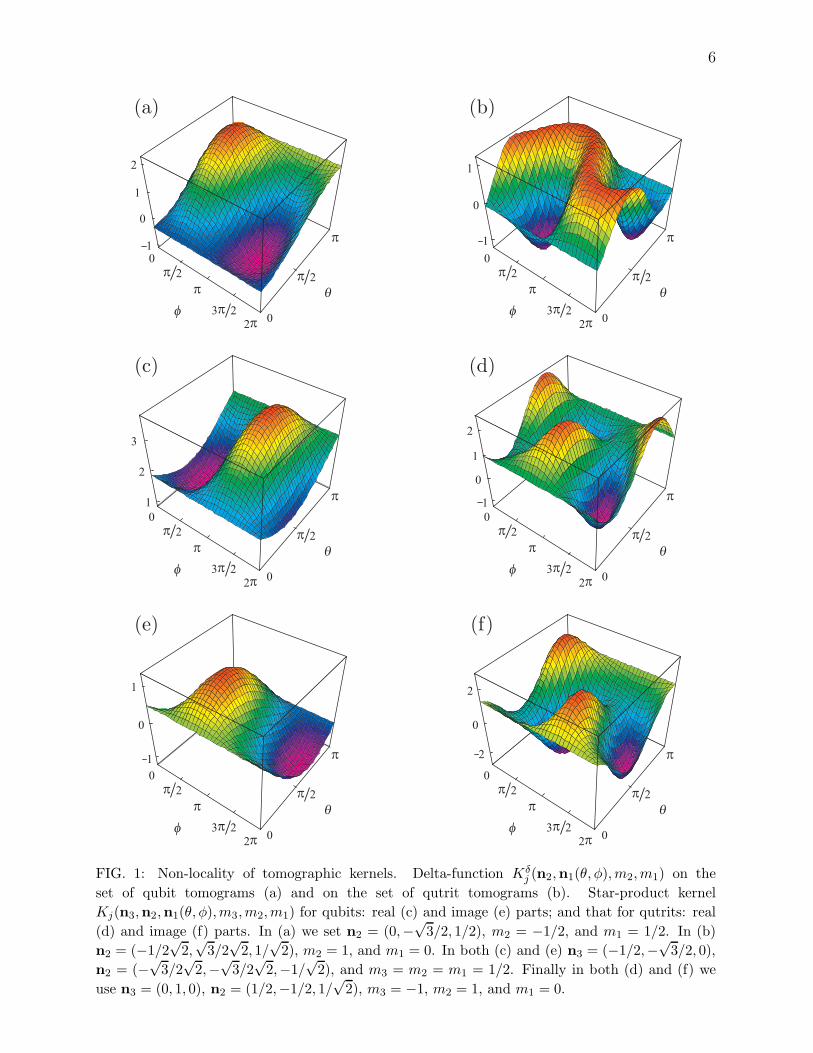
can be treated as the kernel of the unity operator on the set of spin tomograms and plays therole of an analogue of the Dirac delta-function. Some examples of the star-product kernelsand the delta-functions for the low-spin states are depicted in Fig. 1. It is readily seenthat apart from being non-local, the delta-function on the tomogram set is not non-negativeeither.

By analogy with ordinary tomographic symbols, one can also introduce the dual spin-tomographic star-product

fdAB

(x) = fdA(x) ⋆ fd

B(x) (18)

with the non-local kernel of the form

Kdj (x3,x2,x1) = Tr

(

Uj(x3)Uj(x2)Dj(x1))

. (19)

Let us calculate the explicit form of the star-product kernel (15) for qudits with spin j.Using the exponential representation of the dequantizer (5) and the quantizer (9), we

obtain

Kj(x3,x2,x1) =(2j + 1)2

(2π)3

1∑

s2=−1

1∑

s3=−1

1

(1 − 3s22)(1 − 3s2

3)

×2π∫

0

2π∫

0

2π∫

0

Tr(

e−i(n3·J)ϕ3e−i(n2·J)ϕ2e−i(n1·J)ϕ1

)

eim1ϕ1ei(m2+s2)ϕ2ei(m3+s3)ϕ3dϕ1dϕ2dϕ3. (20)

From this it follows that the spin-tomographic star-product kernel (15) is nothing else butthe Fourier transform of SU(2) irreducible representation character

χ(n3,n2,n1, ϕ3, ϕ2, ϕ1) = Tr(

e−i(n3·J)ϕ3e−i(n2·J)ϕ2e−i(n1·J)ϕ1

)

= Tr(

e−i(N·J)Φ)

, (21)

6

2

1

0

1

2

2

2

23

0

0

2

1

0

1

2

2

2

23

0

0

1

0

1

2

2

2

23

0

0

2

3

1

2

2

2

23

0

0

1

0

1

2

2

2

23

0

0

2

0

2

2

2

2

23

0

0

(a) (b)

(c) (d)

(e) (f)

FIG. 1: Non-locality of tomographic kernels. Delta-function Kδj (n2,n1(θ, φ),m2,m1) on the

set of qubit tomograms (a) and on the set of qutrit tomograms (b). Star-product kernel

Kj(n3,n2,n1(θ, φ),m3,m2,m1) for qubits: real (c) and image (e) parts; and that for qutrits: real

(d) and image (f) parts. In (a) we set n2 = (0,−√

3/2, 1/2), m2 = −1/2, and m1 = 1/2. In (b)

n2 = (−1/2√

2,√

3/2√

2, 1/√

2), m2 = 1, and m1 = 0. In both (c) and (e) n3 = (−1/2,−√

3/2, 0),

n2 = (−√

3/2√

2,−√

3/2√

2,−1/√

2), and m3 = m2 = m1 = 1/2. Finally in both (d) and (f) we

use n3 = (0, 1, 0), n2 = (1/2,−1/2, 1/√

2), m3 = −1, m2 = 1, and m1 = 0.

7

where Φ = Φ(n1,n2,n3, ϕ1, ϕ2, ϕ3) and N = N(n1,n2,n3, ϕ1, ϕ2, ϕ3) are respectively theangle and axis of the resulting rotation which is equivalent to successive rotations aroundaxis nk by angle ϕk, k = 1, 2, 3.

To simplify formulas let us introduce the 3-vector ϕ with components (ϕ1, ϕ2, ϕ3) andthe 9-vector N with components constructed from components of three vectors n1, n2, n3,i.e., N = (n1,n2,n3). Also, we designate

∫

dϕ =

2π∫

0

2π∫

0

2π∫

0

dϕ1dϕ2dϕ3, m = (m1, m2, m3). (22)

Given the angle Φ, the character has a rather simple form

χ(Φ) =

j∑

m=−j

eimΦ =sin((2j + 1)Φ/2)

sin(Φ/2)= U2j

(

cos(Φ/2))

, (23)

where Un(cos θ) = sin (n+1)θsin θ

is the Chebyshev polynomial of the second kind of degree n[37, 38].

Thus, combining (20)–(23), we obtain the integral representation of the star-productkernel

Kj(x3,x2,x1) =(2j + 1)2

(2π)3

1∑

s2=−1

1∑

s3=−1

1

(1 − 3s22)(1 − 3s2

3)Ij(x3,x2,x1), (24)

where by Ij(x3,x2,x1) we denote the following integral:

Ij(x3,x2,x1) =

∫

U2j

(

cosΦ(N, ϕ)

2

)

ei(m·ϕ)eis2ϕ2eis3ϕ3dϕ. (25)

This implies that the kernel of spin-tomographic star-product can be treated as the Fouriertransform of the Chebyshev polynomial of a specific argument. In the same way, it caneasily be checked that the kernel of the dual spin-tomographic star-product reads

Kdj (x3,x2,x1) =

2j + 1

(2π)3

1∑

s1=−1

1

1 − 3s21

∫

U2j

(

cosΦ(N, ϕ)

2

)

ei(m·ϕ)eis1ϕ1dϕ. (26)

Further, the angle Φ does not depend on spin j. Consequently it is possible to calculateit for qubits and then extend the obtained result to other spins. Substituting 1/2 for j in(23), we get the character for qubits

χ1/2(Φ) = U1

(

cos(Φ/2))

= 2 cos(Φ/2). (27)

On the other hand, from (21) it follows that

χ1/2(Φ) = Tr(

e−i(n3·σ)ϕ3/2e−i(n2·σ)ϕ2/2e−i(n1·σ)ϕ1/2)

, (28)

where σ = (σx, σy, σz) is a set of the Pauli matrices. Employing the known property of Pauli

matrices σασβ = δαβ 1 + iεαβγ σγ , it is not hard to prove that the relations

8

(a · σ)(b · σ) = aαbβ σασβ = (a · b)1 + i(

[a× b] · σ)

, (29)

e−i(n·σ)ϕ/2 = 1 cos(ϕ/2) − i(n · σ) sin(ϕ/2) (30)

are valid whenever n2 is equal to unity. In view of these relations, we finally obtain

e−i(n3·σ)ϕ3/2e−i(n2·σ)ϕ2/2e−i(n1·σ)ϕ1/2 = 1 cos (Φ(N, ϕ)/2) − i(N · σ) sin (Φ(N, ϕ)/2) . (31)

Recall that the angle Φ depends on three rotation angles ϕ1, ϕ2, ϕ3 and three directions n1,n2, n3. Departing from this notation, one can easily derive the resulting rotation angle

cos (Φ(N, ϕ)/2) = cos(ϕ1/2) cos(ϕ2/2) cos(ϕ3/2) − (n1 · n2) sin(ϕ1/2) sin(ϕ2/2) cos(ϕ3/2)

−(n2 · n3) cos(ϕ1/2) sin(ϕ2/2) sin(ϕ3/2) − (n3 · n1) sin(ϕ1/2) cos(ϕ2/2) sin(ϕ3/2)

+ (n1 · [n2 × n3]) sin(ϕ1/2) sin(ϕ2/2) sin(ϕ3/2) (32)

and the rotation axis

N sin (Φ(N, ϕ)/2) = n1 sin(ϕ1/2) cos(ϕ2/2) cos(ϕ3/2)

+n2 cos(ϕ1/2) sin(ϕ2/2) cos(ϕ3/2) + n3 cos(ϕ1/2) cos(ϕ2/2) sin(ϕ3/2)

−

n1(n2 · n3) − n2(n1 · n3) + n3(n1 · n2)

sin(ϕ1/2) sin(ϕ2/2) sin(ϕ3/2)

−[n1 × n2] sin(ϕ1/2) sin(ϕ2/2) cos(ϕ3/2) − [n2 × n3] cos(ϕ1/2) sin(ϕ2/2) sin(ϕ3/2)

−[n1 × n3] sin(ϕ1/2) cos(ϕ2/2) sin(ϕ3/2). (33)

Now, when cos (Φ(N, ϕ)/2) is known, integral (25) can be evaluated. Change of variablestk = − cot(ϕk/2), k = 1, 2, 3 results in the integral taking the form

Ij(x3,x2,x1) = 8

∫

+∞∫

−∞

∫

dt1dt2dt3(t3 − i)m3+s3−1(t2 − i)m2+s2−1(t1 − i)m1−1

(t3 + i)m3+s3+1(t2 + i)m2+s2+1(t1 + i)m1+1

×U2j

(

t1t2t3 − t1(n2 · n3) − t2(n3 · n1) − t3(n1 · n2) − (n1 · [n2 × n3])

(t1 − i)1/2(t1 + i)1/2(t2 − i)1/2(t2 + i)1/2(t3 − i)1/2(t3 + i)1/2

)

, (34)

where z1/2, z ∈ C is regarded as a principal branch of the square root function, with thebranch cut being along the positive real axis. Since the integrand decreases fast enough as|tk| → ∞, k = 1, 2, 3, one can calculate the integral in question with the help of the residuetheorem. Indeed, choosing for each complex variable tk, k = 1, 2, 3 the path of integrationshown in Fig. 2, we have Ij(x3,x2,x1) = (2πi)3Rest1=iRest2=iRest3=i. In order to calculatethe residues one needs to find a coefficient corresponding to the term (t1− i)−1(t2− i)−1(t3−i)−1.

Employing the expansion of the Chebyshev polynomial

U2j(x) =

[j]∑

k=0

(−1)k(2j − k)!

k!(2j − 2k)!(2x)2j−2k, (35)

9

x

y

i

i

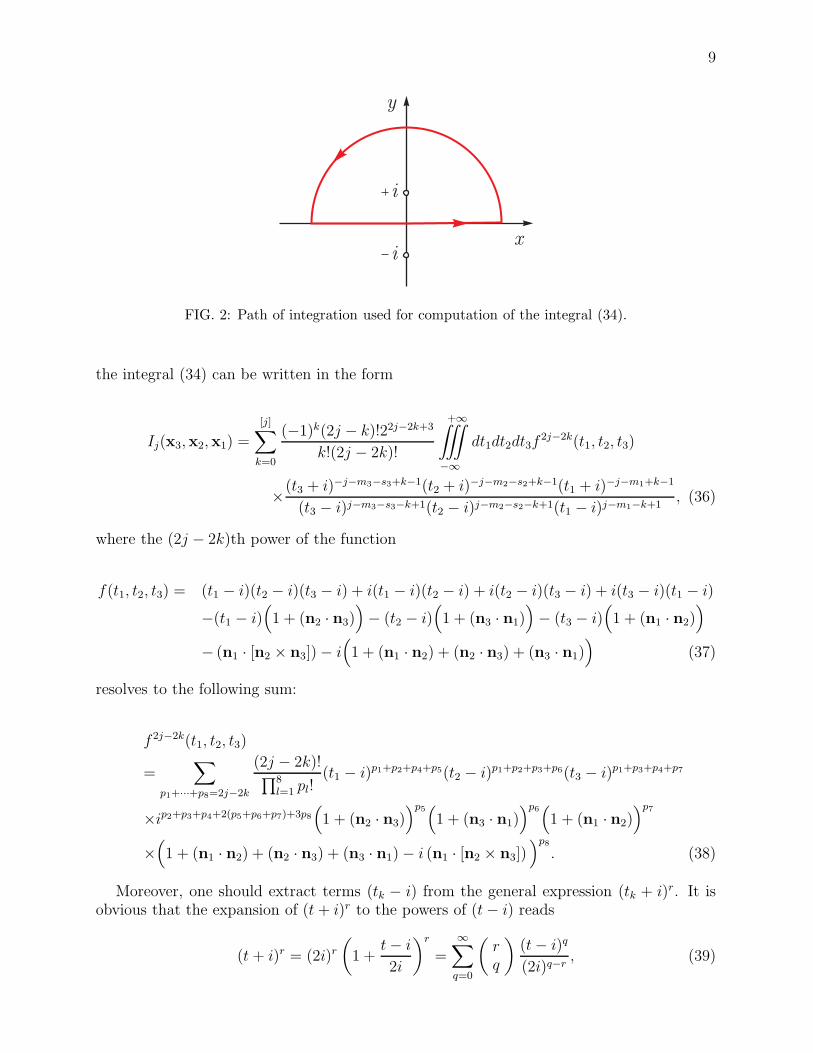
FIG. 2: Path of integration used for computation of the integral (34).

the integral (34) can be written in the form

Ij(x3,x2,x1) =

[j]∑

k=0

(−1)k(2j − k)!22j−2k+3

k!(2j − 2k)!

∫

+∞∫

−∞

∫

dt1dt2dt3f2j−2k(t1, t2, t3)

×(t3 + i)−j−m3−s3+k−1(t2 + i)−j−m2−s2+k−1(t1 + i)−j−m1+k−1

(t3 − i)j−m3−s3−k+1(t2 − i)j−m2−s2−k+1(t1 − i)j−m1−k+1, (36)

where the (2j − 2k)th power of the function

f(t1, t2, t3) = (t1 − i)(t2 − i)(t3 − i) + i(t1 − i)(t2 − i) + i(t2 − i)(t3 − i) + i(t3 − i)(t1 − i)

−(t1 − i)(

1 + (n2 · n3))

− (t2 − i)(

1 + (n3 · n1))

− (t3 − i)(

1 + (n1 · n2))

− (n1 · [n2 × n3]) − i(

1 + (n1 · n2) + (n2 · n3) + (n3 · n1))

(37)

resolves to the following sum:

f 2j−2k(t1, t2, t3)

=∑

p1+···+p8=2j−2k

(2j − 2k)!∏8

l=1 pl!(t1 − i)p1+p2+p4+p5(t2 − i)p1+p2+p3+p6(t3 − i)p1+p3+p4+p7

×ip2+p3+p4+2(p5+p6+p7)+3p8

(

1 + (n2 · n3))p5

(

1 + (n3 · n1))p6

(

1 + (n1 · n2))p7

×(

1 + (n1 · n2) + (n2 · n3) + (n3 · n1) − i (n1 · [n2 × n3]))p8

. (38)

Moreover, one should extract terms (tk − i) from the general expression (tk + i)r. It isobvious that the expansion of (t + i)r to the powers of (t − i) reads

(t + i)r = (2i)r

(

1 +t − i

2i

)r

=

∞∑

q=0

(

rq

)

(t − i)q

(2i)q−r, (39)

10

where we introduced binomial coefficients according to the rule [43]

(

rq

)

=r(r − 1) . . . (r − q + 1)

q!. (40)

Here r is supposed to be real, q is an integer,

(

rq

)

= 0 if q < 0, and

(

r0

)

= 1.

If we combine (36) with (38) and (39), we can calculate the residues involved and thenthe integral I. The direct computation yields

Ij(x3,x2,x1)

= (2π)3

[j]∑

k=0

∑

p1+···+p8=2j−2k

(−1)k(2j − k)!22j−2k+3

k!∏8

l=1 pl!

(

1 + (n2 · n3))p5

(

1 + (n3 · n1))p6

×(

1 + (n1 · n2))p7

(

1 + (n1 · n2) + (n2 · n3) + (n3 · n1) − i (n1 · [n2 × n3]))p8

×∞

∑

q3=0

∞∑

q2=0

∞∑

q1=0

ip2+p3+p4+2(p5+p6+p7)+3p8+3

(2i)3j+m3+m2+m1+s3+s2−3k+3+q3+q2+q1

(

−j − m1 + k − 1q1

)

×(

−j − m2 − s2 + k − 1q2

) (

−j − m3 − s3 + k − 1q3

)

×δj−m1−k−p1−p2−p4−p5−q1,0δj−m2−s2−k−p1−p2−p3−p6−q2,0δj−m3−s3−k−p1−p3−p4−p7−q3,0. (41)

Finally, substituting the calculated value of I for the integral in (24), we obtain the explicitform of the spin-tomographic star-product kernel

Kj(x3,x2,x1)

= (2j + 1)21

∑

s3=−1

1∑

s2=−1

[j]∑

k=0

∑

p1+···+p8=2j−2k

(−1)k(2j − k)!

(1 − 3s23)(1 − 3s2

2)2−p1+p5+p6+p7+2p8k!

∏8l=1 pl!

×(

1 + (n2 · n3))p5

(

1 + (n3 · n1))p6

(

1 + (n1 · n2))p7

×(

1 + (n1 · n2) + (n2 · n3) + (n3 · n1) − i (n1 · [n2 × n3]))p8

×(

−j − m1 + k − 1j − m1 − k − p1 − p2 − p4 − p5

) (

−j − m2 − s2 + k − 1j − m2 − s2 − k − p1 − p2 − p3 − p6

)

×(

−j − m3 − s3 + k − 1j − m3 − s3 − k − p1 − p3 − p4 − p7

)

. (42)

IV. EQUIVALENCY OF KERNEL REPRESENTATIONS

The problem of the explicit form of the star-product kernel has been attacked fromdifferent perspectives. In the work [27], the explicit formula is expressed in terms of Clebsch-Gordan and Racah coefficients. To be more precise, the result is

11

K′j(x3,x2,x1) = (−1)j−m1−m2−m3

2j∑

L1=0

2j∑

L2=0

2j∑

L3=0

(−1)L1+L2+L3

√

(2L3 + 1)3(2L2 + 1)3(2L1 + 1)

×〈jm1; j − m1|L10〉〈jm2; j − m2|L20〉〈jm3; j − m3|L30〉

L2 L3 L1

j j j

×L1∑

M1=−L1

L2∑

M2=−L2

L3∑

M3=−L3

(

L2 L3 L1

M2 M3 M1

)

D(L1)0−M1

(0, θ1,−φ1)D(L2)0−M2

(0, θ2,−φ2)D(L3)0−M3

(0, θ3,−φ3),

(43)

where the Wigner D-function reads

D(j)m′m(α, β, γ) = e−im′αe−imγ

∑

s

(−1)s√

(j + m)!(j − m)!(j + m′)!(j − m′)!

s!(j − m′ − s)!(j + m − s)!(m′ − m + s)!

×(

cosβ

2

)2j+m−m′−2s (

− sinβ

2

)m′−m+2s

. (44)

In [28], using the irreducible tensor operators for the SU(2) group [39, 40], the same resultis specified for the low-spin states and presented in the form of the expansion to orthog-onal summands. In the present work, starting from the exponential representation of thequantizer and dequantizer operators, we managed to obtain another explicit form of thestar-product kernel which can also be presented in the form

K′′j (x3,x2,x1)

= (2j + 1)2

1∑

s3=−1

1∑

s2=−1

[j]∑

k=0

∑

p1+···+p8=2j−2k

(−1)k(2j − k)!

(1 − 3s23)(1 − 3s2

2)2−p1+p5+p6+p7+2p8k!

∏8l=1 pl!

×(

1 + (n(θ2, φ2) · n(θ3, φ3)))p5

(

1 + (n(θ3, φ3) · n(θ1, φ1)))p6

(

1 + (n(θ1, φ1) · n(θ2, φ2)))p7

×(

1 + (n(θ1, φ1) · n(θ2, φ2)) + (n(θ2, φ2) · n(θ3, φ3)) + (n(θ3, φ3) · n(θ1, φ1))

−i (n(θ1, φ1) · [n(θ2, φ2) × n(θ3, φ3)]))p8

×(

−j − m1 + k − 1j − m1 − k − p1 − p2 − p4 − p5

) (

−j − m2 − s2 + k − 1j − m2 − s2 − k − p1 − p2 − p3 − p6

)

×(

−j − m3 − s3 + k − 1j − m3 − s3 − k − p1 − p3 − p4 − p7

)

. (45)

It is obvious that all the different formulas must be equivalent on the set of tomograms.This is followed by a specific sum rule for Clebsch-Gordan and Racah coefficients. Namely

K′j(x3,x2,x1) ∼ K′′

j (x3,x2,x1), (46)

where the sign ∼ is defined through a biconditional implication of the form

12

K′j(x3,x2,x1) ∼ K′′

j (x3,x2,x1) ⇐⇒

∫∫

fA(x3)fB(x2)K′j(x3,x2,x1)dx2dx3

=

∫∫

fA(x3)fB(x2)K′′j (x3,x2,x1)dx2dx3 for all symbols fA(x) and fB(x)

. (47)

Some of sum rules for Clebsch-Gordan coefficients can be found in [39, 41, 42].Though there takes place an ambiguity in the star-product kernel, all types of the kernel

must be equivalent for calculating the symbol of the product of two given operators. Asfar as functions (43) and (45) are concerned, in case of qubits (j = 1/2), both formulasturned out to be the same (and consequently equal to that found in [28]). In case of qutrits(j = 1), the kernel (45) contains more terms than the kernel (43) expressed in terms ofClebsch-Gordan coefficients. Actually, all redundant terms give zero while integrating withtomographic symbols. In Appendix 1, we discuss the cause of the deviation between kernelsand present the difference ∆j = K′′

j (x3,x2,x1) −K′j(x3,x2,x1) for qutrits (j = 1).

V. RECURRENCE RELATION FOR SPIN-TOMOGRAPHIC KERNELS

The Chebyshev polynomials obey the recurrence relation of the form [37, 38]

Un+1(x) = 2xUn(x) − Un−1(x). (48)

Using this peculiar property of the Chebyshev polynomials, it is easy to prove that thereexists a similar recurrence relation for integral (25). In fact, one has

Ij+1/2(x3,x2,x1) = 2Jj(x3,x2,x1) − Ij−1/2(x3,x2,x1), (49)

where

Jj(x3,x2,x1) =

[j]∑

k=0

(−1)k(2j − k)!22j−2k+3

k!(2j − 2k)!

∫

+∞∫

−∞

∫

dt1dt2dt3f2j−2k+1(t1, t2, t3)

×(t3 + i)−j−m3−s3+k−3/2(t2 + i)−j−m2−s2+k−3/2(t1 + i)−j−m1+k−3/2

(t3 − i)j−m3−s3−k+3/2(t2 − i)j−m2−s2−k+3/2(t1 − i)j−m1−k+3/2. (50)

Employing the explicit form (37) of the function f(t1, t2, t3), one can calculate the integralinvolved just in the same way as it was fulfilled before and then utilize the following propertyof binomial coefficients [43]:

(

rq + 1

)

=

(

r + 1q + 1

)

−(

rq

)

. (51)

The result is

13

Jj(x3,x2,x1) =∑

m′

1,m′

2,m′

3

Ij(N,m′)

[

δm′

1,m1+1/2 δm′

2,m2+1/2 δm′

3,m3+1/2

+1

2

∑

k<l

∑

h 6=k,l

1/2∑

ν=−1/2

(−1)1/2+νδm′

h,mh+ν δm′

k,mk+1/2 δm′

l,ml+1/2

+1

4

∑

k<l

∑

h 6=k,l

(

1 + (nk · nl))

1/2∑

νk=−1/2

1/2∑

νl=−1/2

(−1)1+νk+νlδm′

h,mh+1/2 δm′

k,mk+νk

δm′

l,ml+νl

+1

8

(

1 + (n1 · n2) + (n2 · n3) + (n3 · n1) − i (n1 · [n2 × n3]))

×1/2∑

ν1=−1/2

1/2∑

ν2=−1/2

1/2∑

ν3=−1/2

(−1)3/2+ν1+ν2+ν3δm′

1,m1+ν1

δm′

2,m2+ν2

δm′

3,m3+ν3

]

. (52)

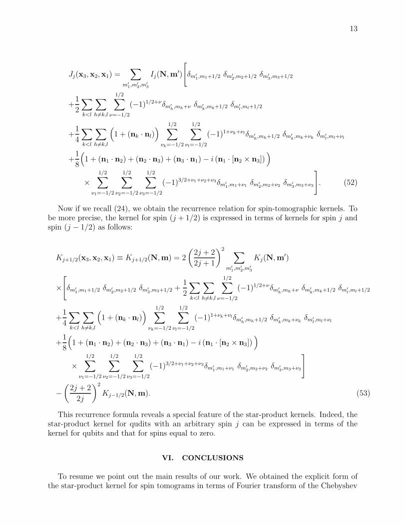
Now if we recall (24), we obtain the recurrence relation for spin-tomographic kernels. Tobe more precise, the kernel for spin (j + 1/2) is expressed in terms of kernels for spin j andspin (j − 1/2) as follows:

Kj+1/2(x3,x2,x1) ≡ Kj+1/2(N,m) = 2

(

2j + 2

2j + 1

)2∑

m′

1,m′

2,m′

3

Kj(N,m′)

×[

δm′

1,m1+1/2 δm′

2,m2+1/2 δm′

3,m3+1/2 +

1

2

∑

k<l

∑

h 6=k,l

1/2∑

ν=−1/2

(−1)1/2+νδm′

h,mh+ν δm′

k,mk+1/2 δm′

l,ml+1/2

+1

4

∑

k<l

∑

h 6=k,l

(

1 + (nk · nl))

1/2∑

νk=−1/2

1/2∑

νl=−1/2

(−1)1+νk+νlδm′

h,mh+1/2 δm′

k,mk+νk

δm′

l,ml+νl

+1

8

(

1 + (n1 · n2) + (n2 · n3) + (n3 · n1) − i (n1 · [n2 × n3]))

×1/2∑

ν1=−1/2

1/2∑

ν2=−1/2

1/2∑

ν3=−1/2

(−1)3/2+ν1+ν2+ν3δm′

1,m1+ν1

δm′

2,m2+ν2

δm′

3,m3+ν3

]

−(

2j + 2

2j

)2

Kj−1/2(N,m). (53)

This recurrence formula reveals a special feature of the star-product kernels. Indeed, thestar-product kernel for qudits with an arbitrary spin j can be expressed in terms of thekernel for qubits and that for spins equal to zero.

VI. CONCLUSIONS

To resume we point out the main results of our work. We obtained the explicit form ofthe star-product kernel for spin tomograms in terms of Fourier transform of the Chebyshev

14

polynomial (see Eqs. (24) and (25)). The expllcit form of the recurrence relation for spin-tomographic star-product kernels is another new result of the work. This relation providesa connection of the kernels for qudits (j ≥ 1) with two basic kernels for the cases j = 0 andj = 1/2. We clarified the relations between different forms of quantizers and dequantizersused in spin tomography and available in the literature [15, 16, 27, 29]. We establishedthat all the different expressions for the quantizers and dequantizers are equivalent on theset of tomographic symbols for the spin operators and spin states. The kernel of the dualtomographic star-product is also expressed in terms of Chebyshev polynomials (see Eq. (26))and calculated explicitly (see Eq.(B3)). Within the proposed technique, we also managedto obtain explicit expressions for delta-function on the tomogram set. In the work [44], therelation of irreps characters for compact and finite groups with kernels of star-products ofthe functions on the groups was obtained. In the present work, we found the relation ofthe characters of SU(2)-group irreps with the star-product of functions depending on bothgroup element and weight of irreps.

Acknowledgments

V.I.M. thanks the Russian Foundation for Basic Research for partial support underProject Nos. 07-02-00598 and 08-02-90300. S.N.F. thanks the Ministry of Education andScience of the Russian Federation and the Federal Education Agency for support underProject No. 2.1.1/5909.

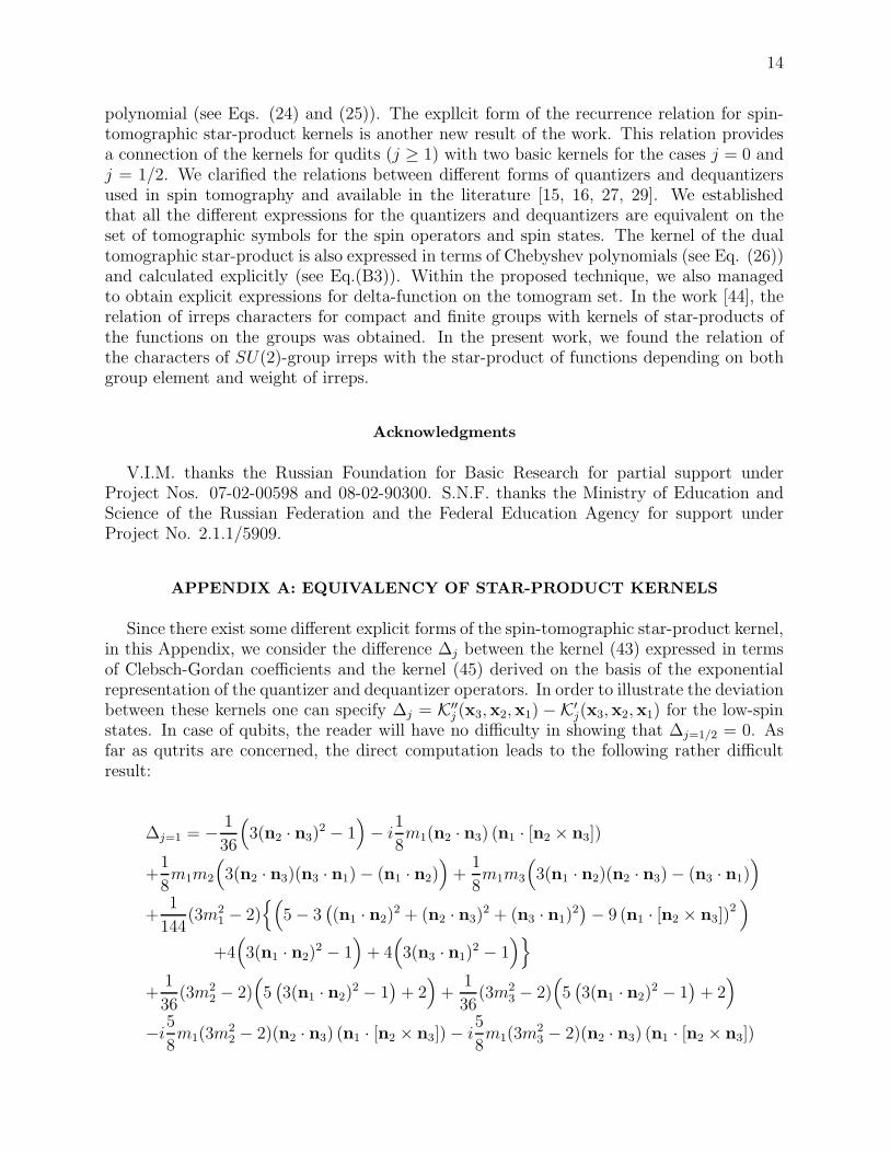
APPENDIX A: EQUIVALENCY OF STAR-PRODUCT KERNELS

Since there exist some different explicit forms of the spin-tomographic star-product kernel,in this Appendix, we consider the difference ∆j between the kernel (43) expressed in termsof Clebsch-Gordan coefficients and the kernel (45) derived on the basis of the exponentialrepresentation of the quantizer and dequantizer operators. In order to illustrate the deviationbetween these kernels one can specify ∆j = K′′

j (x3,x2,x1) − K′j(x3,x2,x1) for the low-spin

states. In case of qubits, the reader will have no difficulty in showing that ∆j=1/2 = 0. Asfar as qutrits are concerned, the direct computation leads to the following rather difficultresult:

∆j=1 = − 1

36

(

3(n2 · n3)2 − 1

)

− i1

8m1(n2 · n3) (n1 · [n2 × n3])

+1

8m1m2

(

3(n2 · n3)(n3 · n1) − (n1 · n2))

+1

8m1m3

(

3(n1 · n2)(n2 · n3) − (n3 · n1))

+1

144(3m2

1 − 2)(

5 − 3(

(n1 · n2)2 + (n2 · n3)

2 + (n3 · n1)2)

− 9 (n1 · [n2 × n3])2)

+4(

3(n1 · n2)2 − 1

)

+ 4(

3(n3 · n1)2 − 1

)

+1

36(3m2

2 − 2)(

5(

3(n1 · n2)2 − 1

)

+ 2)

+1

36(3m2

3 − 2)(

5(

3(n1 · n2)2 − 1

)

+ 2)

−i5

8m1(3m

22 − 2)(n2 · n3) (n1 · [n2 × n3]) − i

5

8m1(3m

23 − 2)(n2 · n3) (n1 · [n2 × n3])

15

−i3

8(3m2

1 − 2)m2(n3 · n1) (n1 · [n2 × n3]) − i3

8(3m2

1 − 2)m3(n1 · n2) (n1 · [n2 × n3])

+1

4m1m2(3m

23 − 2)(n1 · n2) +

1

4m1(3m

22 − 2)m3(n3 · n1) +

1

36(3m2

2 − 2)(3m23 − 2)

+1

144(3m2

1 − 2)(3m22 − 2)

2(

3(n3 · n1)2 − 1

)

+5(

5 − 3(

(n1 · n2)2 + (n2 · n3)

2 + (n3 · n1)2)

− 9 (n1 · [n2 × n3])2)

+1

144(3m2

1 − 2)(3m23 − 2)

2(

3(n1 · n2)2 − 1

)

+5(

5 − 3(

(n1 · n2)2 + (n2 · n3)

2 + (n3 · n1)2)

− 9 (n1 · [n2 × n3])2)

+5

72(3m2

1 − 2)(3m22 − 2)(3m2

3 − 2)(

(

3(n1 · n2)2 − 1

)

+(

3(n3 · n1)2 − 1

)

)

. (A1)

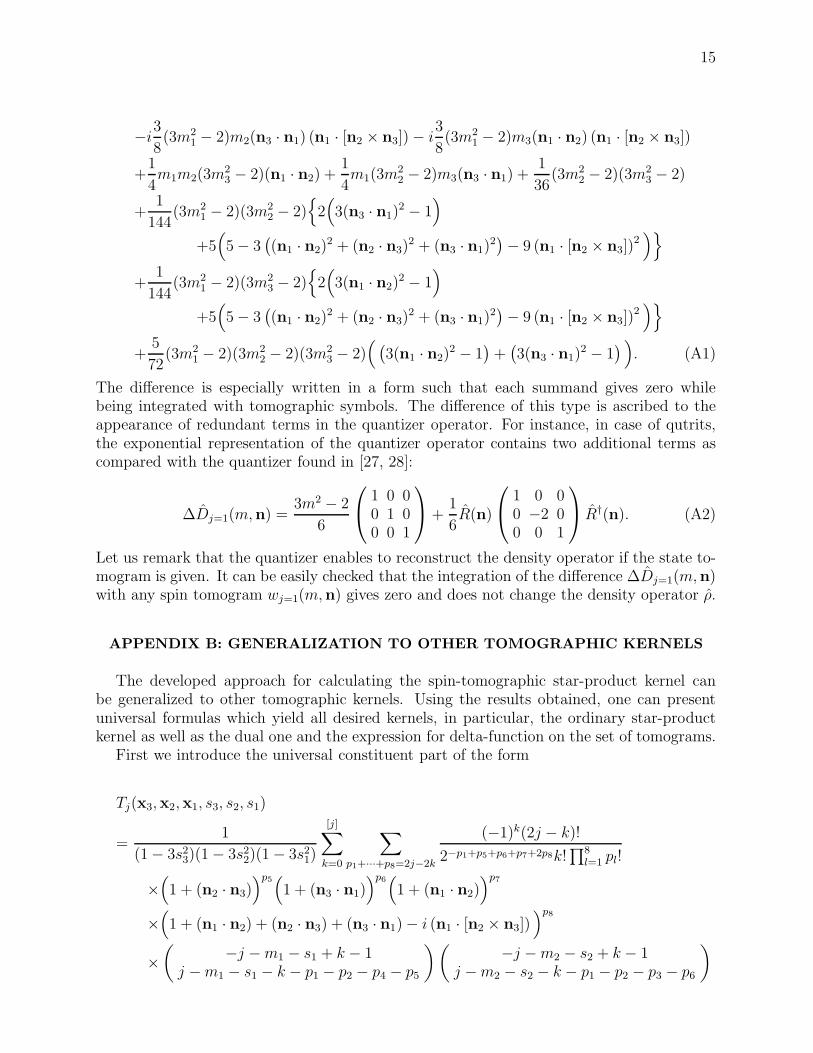
The difference is especially written in a form such that each summand gives zero whilebeing integrated with tomographic symbols. The difference of this type is ascribed to theappearance of redundant terms in the quantizer operator. For instance, in case of qutrits,the exponential representation of the quantizer operator contains two additional terms ascompared with the quantizer found in [27, 28]:

∆Dj=1(m,n) =3m2 − 2

6

1 0 00 1 00 0 1

+1

6R(n)

1 0 00 −2 00 0 1

R†(n). (A2)

Let us remark that the quantizer enables to reconstruct the density operator if the state to-mogram is given. It can be easily checked that the integration of the difference ∆Dj=1(m,n)with any spin tomogram wj=1(m,n) gives zero and does not change the density operator ρ.

APPENDIX B: GENERALIZATION TO OTHER TOMOGRAPHIC KERNELS

The developed approach for calculating the spin-tomographic star-product kernel canbe generalized to other tomographic kernels. Using the results obtained, one can presentuniversal formulas which yield all desired kernels, in particular, the ordinary star-productkernel as well as the dual one and the expression for delta-function on the set of tomograms.

First we introduce the universal constituent part of the form

Tj(x3,x2,x1, s3, s2, s1)

=1

(1 − 3s23)(1 − 3s2

2)(1 − 3s21)

[j]∑

k=0

∑

p1+···+p8=2j−2k

(−1)k(2j − k)!

2−p1+p5+p6+p7+2p8k!∏8

l=1 pl!

×(

1 + (n2 · n3))p5

(

1 + (n3 · n1))p6

(

1 + (n1 · n2))p7

×(

1 + (n1 · n2) + (n2 · n3) + (n3 · n1) − i (n1 · [n2 × n3]))p8

×(

−j − m1 − s1 + k − 1j − m1 − s1 − k − p1 − p2 − p4 − p5

) (

−j − m2 − s2 + k − 1j − m2 − s2 − k − p1 − p2 − p3 − p6

)

16

×(

−j − m3 − s3 + k − 1j − m3 − s3 − k − p1 − p3 − p4 − p7

)

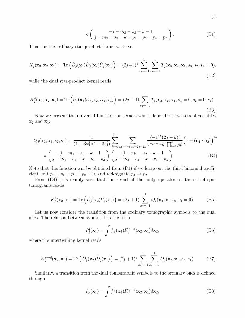
. (B1)

Then for the ordinary star-product kernel we have

Kj(x3,x2,x1) = Tr(

Dj(x3)Dj(x2)Uj(x1))

= (2j+1)21

∑

s3=−1

1∑

s2=−1

Tj(x3,x2,x1, s3, s2, s1 = 0),

(B2)while the dual star-product kernel reads

Kdj (x3,x2,x1) = Tr

(

Uj(x3)Uj(x2)Dj(x1))

= (2j + 1)1

∑

s1=−1

Tj(x3,x2,x1, s3 = 0, s2 = 0, s1).

(B3)Now we present the universal function for kernels which depend on two sets of variables

x2 and x1:

Qj(x2,x1, s2, s1) =1

(1 − 3s22)(1 − 3s2

1)

[j]∑

k=0

∑

p1+···+p4=2j−2k

(−1)k(2j − k)!

2−p1+p4k!∏4

l=1 pl!

(

1 + (n1 · n2))p4

×(

−j − m1 − s1 + k − 1j − m1 − s1 − k − p1 − p2

) (

−j − m2 − s2 + k − 1j − m2 − s2 − k − p1 − p3

)

. (B4)

Note that this function can be obtained from (B1) if we leave out the third binomial coeffi-cient, put p2 = p5 = p6 = p8 = 0, and redesignate p4 → p2.

From (B4) it is readily seen that the kernel of the unity operator on the set of spintomograms reads

Kδj (x2,x1) = Tr

(

Dj(x2)Uj(x1))

= (2j + 1)1

∑

s2=−1

Qj(x2,x1, s2, s1 = 0). (B5)

Let us now consider the transition from the ordinary tomographic symbols to the dualones. The relation between symbols has the form

fdA(x1) =

∫

fA(x2)Ko→dj (x2,x1)dx2, (B6)

where the intertwining kernel reads

Ko→dj (x2,x1) = Tr

(

Dj(x2)Dj(x1))

= (2j + 1)2

1∑

s2=−1

1∑

s1=−1

Qj(x2,x1, s2, s1). (B7)

Similarly, a transition from the dual tomographic symbols to the ordinary ones is definedthrough

fA(x1) =

∫

fdA(x2)K

d→oj (x2,x1)dx2, (B8)

17

where the intertwining kernel reads

Kd→oj (x2,x1) = Tr

(

Uj(x2)Uj(x1))

= Qj(x2,x1, s2 = 0, s1 = 0). (B9)

[1] E. P. Wigner, Phys. Rev., 40, 749 (1932).

[2] K. Husimi, Proc. Phys. Math. Soc. Jpn., 22, 264 (1940).

[3] S. Mancini, V. I. Man’ko, and P. Tombesi, Phys. Lett. A, 213, 1 (1996).

[4] V. I. Man’ko, G. Marmo, A. Simoni, E. C. G. Sudarshan, and F. Ventriglia, Rep. Math. Phys.,

61, 337 (2008).

[5] J. Bertrand and P. Bertrand, Found. Phys., 17, 397 (1987).

[6] K. Vogel and H. Risken, Phys. Rev. A, 40, 2847 (1989).

[7] V. I. Man’ko and R. V. Mendes, Physica D, 145, 330 (2000).

[8] O. Man’ko and V. I. Man’ko, J. Russ. Laser Res., 18, 407 (1997).

[9] O. V. Man’ko, V. I. Man’ko, and G. Marmo, J. Phys. A: Math. Gen., 35, 699 (2002).

[10] D. T. Smithey, M. Beck, M. G. Raymer, and A. Faridani, Phys. Rev. Lett., 70, 1244 (1993).

[11] J. Mlynek, Phys. Rev. Lett., 77, 2933 (1996).

[12] A. I. Lvovsky, H. Hansen, T. Alchele, O. Benson, J. Mlynek, and S. Schiller, Phys. Rev. Lett.,

87, 050402 (2001).

[13] V. D’Auria, S. Fornaro, A. Porzio, S. Solimeno, S. Olivares, and M. G. A. Paris, Phys. Rev.

Lett., 102, 020502 (2009).

[14] T. Kiesel, W. Vogel, V. Parigi, A. Zavatta, and M. Bellini, Phys. Rev. A, 78, 021804 (2008).

[15] V. V. Dodonov and V. I. Man’ko, Phys. Lett. A, 229, 335 (1997).

[16] V. I. Man’ko and O. V. Man’ko, J. Exp. Theor. Phys., 85, 430 (1997).

[17] S. Weigert, Phys. Rev. Lett., 84, 802 (2000).

[18] J. P. Amiet and S. Weigert, J. Opt. B: Quantum Semiclass. Opt., 1, L5 (1999).

[19] G. S. Agarwal, Phys. Rev. A, 57, 671 (1998).

[20] C. Munoz, A. B. Klimov, L. L. Sanchez-Soto, and G. Bjork, ”Discrete coherent states for n

qubits,” quant-ph/0809.4995 (2008).

[21] J. F. Carinena, J. M. Garcia-Bondia, and J. C. Varilly, J. Phys. A: Math. Gen., 23, 901

(1990).

[22] A. B. Klimov and J. L. Romero, J. Phys. A: Math. Theor., 41, 055303 (2008).

[23] V. I. Man’ko, G. Marmo, and P. Vitale, Phys. Lett. A, 334, 1 (2005).

[24] O. V. Man’ko, V. I. Man’ko, and G. Marmo, Phys. Scr., 62, 446 (2000).

[25] O. Man’ko, V. I. Man’ko, and G. Marmo, J. Phys. A: Math. Gen., 35, 699 (2002).

[26] O. V. Man’ko, J. Russ. Laser Res., 28, 483 (2007).

[27] O. Castanos, R. Lopez-Pena, M. A. Man’ko, and V. I. Man’ko, J. Phys. A: Math. Gen., 36,

4677 (2003).

[28] S. N. Filippov and V. I. Man’ko, J. Russ. Laser Res., 30, 82 (2009).

[29] G. M. D’Ariano, L. Maccone, and M. Paini, J. Opt. B: Quantum Semicl. Opt., 5, 77 (2003).

[30] V. A. Andreev and V. I. Man’ko, J. Exp. Theor. Phys., 87, 239 (1998).

[31] O. V. Man’ko, V. I. Man’ko, and S. S. Safonov, Theor. Math. Phys., 115, 185 (1998).

[32] V. A. Andreev, O. V. Man’ko, V. I. Man’ko, and S. S. Safonov, J. Russ. Laser Res., 19, 340

(1998).

18

[33] S. N. Filippov and V. I. Man’ko, J. Russ. Laser Res., 29, 564 (2008).

[34] M. A. Man’ko, V. I. Man’ko, and R. V. Mendes, J. Phys. A: Math. Gen., 34, 8321 (2001).

[35] O. V. Man’ko, V. I. Man’ko, G. Marmo, and P. Vitale, Phys. Lett. A, 360, 522 (2007).

[36] S. N. Filippov and V. I. Man’ko, Phys. Scr., 79, 055007 (2009).

[37] H. Bateman and A. Erdelyi, Higher transcendential functions, Volume 2, Mc Graw-Hill Book

Company, New York Toronto London (1953).

[38] I. S. Gradstein and I. M. Ryzhik, Tables of integrals, series and products, Academic Press,

New York (1965).

[39] D. A. Varshalovich, A. N. Moskalev, and V. K. Khersonskii, Theory of Angular Momentum,

World Scientific, Singapore (1988).

[40] A. B. Klimov and S. M. Chumakov, J. Opt. Soc. Am. A, 17, 2315 (2000).

[41] L. A. Shelepin, Tr. Fiz. Inst., Akad. Nauk SSSR, 70, 3 (1973).

[42] Ya. A. Smorodinsky and L. A. Shelepin, Sov. Phys. Usp., 15, 1 (1973).

[43] G. A. Korn and T. M. Korn, Mathematical handbook for scientists and engineers. Definitions,

theorems, and formulas for reference and review, McGraw-Hill, New York, 2nd enl. and rev.

edition (1968), p. 21.5-1.

[44] P. Aniello, A. Ibort, V. I. Man’ko, and G. Marmo, Phys. Lett. A, 373, 401 (2009).