Characterizing the Severe Turbulence Environments Associated With Commercial Aviation Accidents

Meteorol Atmos Phys 94, 235–270 (2006)DOI 10.1007/s00703-005-0181-4

1 Department of Marine, Earth, and Atmospheric Sciences, North Carolina State University, Raleigh, NC, USA2 USDA=Forest Service, North Central Research Station, East Lansing, MI, USA3 MESO Inc., Raleigh, NC, USA

Characterizing the severe turbulence environmentsassociated with commercial aviation accidents. A real-timeturbulence model (RTTM) designed for the operationalprediction of hazardous aviation turbulence environments

M. L. Kaplan1, J. J. Charney2, K. T. Waight III3, K. M. Lux1, J. D. Cetola1,A. W. Huffman1, A. J. Riordan1, S. D. Slusser1, M. T. Kiefer1,P. S. Suffern1, and Y.-L. Lin1

With 19 Figures

Received April 1, 2004; revised April 25, 2005; accepted November 24, 2005Published online: July 31, 2006 # Springer-Verlag 2006

Summary

In this paper, we will focus on the real-time prediction ofenvironments that are predisposed to producing moderate-severe (hazardous) aviation turbulence. We will describe thenumerical model and its postprocessing system that is de-signed for said prediction of environments predisposed tosevere aviation turbulence as well as presenting numerousexamples of its utility. The purpose of this paper is to dem-onstrate that simple hydrostatic precursor circulations orga-nize regions of preferred wave breaking and turbulence at thenonhydrostatic scales of motion. This will be demonstratedwith a hydrostatic numerical modeling system, which can berun in real time on a very inexpensive university computerworkstation employing simple forecast indices. The forecastsystem is designed to efficiently support forecasters who aredirecting research aircraft to measure the environmentimmediately surrounding turbulence.

The numerical model is MASS version 5.13, which is in-tegrated over three different grid matrices in real-time on auniversity workstation in support of NASA-Langley’s B-757turbulence research flight missions. The model horizontalresolutions are 60, 30, and 15 km and the grids are centeredover the region of operational NASA-Langley B-757 turbu-lence flight missions.

The postprocessing system includes several turbulence-related products including four turbulence forecasting indices,winds, streamlines, turbulence kinetic energy, and Richardson

numbers. Additionally there are convective products includ-ing precipitation, cloud height, cloud mass fluxes, lifted index,and K-index. Furthermore, soundings, sounding parameters,and Froude number plots are also provided. The horizontalcross section plot products are provided from 16,000–46,000feet in 2,000 feet intervals. Products are available every threehours at the 60 and 30 km grid interval and every 1.5 hours atthe 15 km grid interval. The model is initialized from theNWS ETA analyses and integrated two times a day.

1. Introduction

The operational forecasting of turbulence poten-tial has been ongoing for several years. Manyindices are generated daily from operational num-erical weather prediction models. The NationalWeather Service has employed the Ellrod Index(e.g., Ellrod and Knapp, 1992), the NOAA Fore-casting Systems Laboratory has employed in-dices developed by Marroqin et al (1990) basedon turbulence kinetic energy and eddy dissipa-tion rate, and the Research Applications Programof the National Center for Atmospheric Researchhad developed the Integrated Turbulence Fore-casting Algorithm (ITFA) index as part of the

suite of products from the NWS RUC II-model(Sharman et al, 2000). This system is now knownas the Graphical Turbulence Guidance (GTG)system. The Ellrod Index is by far the simplestbased solely on deformation and vertical windshear. The Marroquin index is based on a for-mulation of turbulence kinetic energy. GTG is,by far, the most comprehensive and sophisticatedindex, that is used operationally, employing aweighted set of nearly twenty individual compo-nent terms as well as contemporary observationsof turbulence pireps into a turbulence probabilityindex. In spite of the sophistication of GTG it isdesigned primarily for nonconvective turbulence,i.e., clear air turbulence (CAT) and mountainwave-induced turbulence. It is not exclusively de-signed to denote regions of severe turbulence buta broad cross-section of turbulence intensities in-cluding light, moderate, and severe. As noted inKaplan et al (2005a), most severe aviation turbu-lence encounters that result in damage to aircraftor onboard injuries are closely associated withmoist convection. Hence, a turbulence predictiveindex, to be employed on an operational basis,needs to have the capacity to predict not only theenvironments that organize light-moderate turbu-lence, which typically occurs in clear air, but themore severe turbulence most often found in asso-ciation with moist convection, i.e., convectively-induced turbulence (CIT) which is most oftenassociated with aviation accidents. Additionally,one of the negative aspects of GTG, is that it isan amalgamation of so many different specificdynamical terms and empirical weighting factorsthat it is unclear what physical=dynamical pro-cesses are most relevant in organizing the envi-ronment that is favorable for turbulence in a givencase study, particularly severe accident-producingturbulence. Therefore one is dependent upon sta-tistical validation rather than dynamical under-standing when the inevitable improvement of saidindex is undertaken. The use of the much simplerRTTM indices facilitates a clearer understandingof what hydrostatic environments tend to orga-nize fine scale turbulence.

In the remainder of this paper we will demon-strate the utility of the index described in Kaplanet al (2005a, b) in delimiting, in real-time, areas ofmoderate-severe turbulence potential. Addition-ally we will demonstrate that said index has thecapacity to denote all three forms of turbulence

including CAT, CIT and mountain wave-inducedturbulence. We will do so with a hydrostatic nu-merical modeling system that is very inexpensiveto run on a university computer workstation. Inthe next section of the paper we will describe thenumerical modeling system and postprocessoremployed in the Real-Time Turbulence Model(RTTM) run operationally at North Carolina StateUniversity in support of NASA’s B-757 turbu-lence research missions. We will focus on a de-scription of the key turbulence-forecasting indexin this section of the paper. The third section ofthis paper will focus on several real-time examples

Table 1. MASS model (vers. 5.13) characteristics

Model numerics

– Hydrostatic primitive equation model– 3-D equations for u, v, T, q, and p– Cartesian grid on a polar stereographic map– Sigma-p terrain-following vertical coordinate– Vertical coverage from �10 m to �16,000 m– Energy-absorbing sponge layer near model top– Fourth-order horizontal space differencing on an

unstaggered grid– Split–explicit time integration schemes: (a) forward–

backward for the gravity mode and(b) Adams–Bashforth for the advective mode

– Time-dependent lateral boundary conditions– Positive–definite advection scheme for the scalar variables– Massless tracer equations for ozone and aerosol transport

Initialization

– First guess from large-scale gridded analyses– Reanalysis with rawinsonde and surface data using

a 3D optimum interpolation scheme– High-resolution terrain data base derived from

observations– High-resolution satellite or climatological sea surface

temperature database– High-resolution land use classification scheme– High-resolution climatological subsoil moisture data

base derived from antecedent precipitation– High resolution normalized difference vegetation index

PBL specification

– Blackadar PBL scheme– Surface energy budget– Soil hydrology scheme– Atmospheric radiation attenuation scheme

Moisture physics

– Grid-scale prognostic equations for cloud water and ice,rainwater, and snow

– Kain–Fritsch convective parameterization

236 M. L. Kaplan et al

of the model, its index, and simulated precipita-tion and wind fields associated with case studiesof observed turbulence as reported by pireps. Theability of the model to denote CIT will be di-agnosed, in particular, although its versatility indefining regions of both CAT and mountain wave-induced turbulence will also be described. Thefinal section will focus on summarizing the mod-eling system and its application to the problem ofthe real-time forecasting of turbulence potential.It must be reiterated that this system was devel-oped for its efficiency and its convenient use byNASA weather forecasters who are familiar withits predictive indices and with whose collabora-tion these indices were developed. Additionally,its scientific utility is that it demonstrates the keyhydrostatic processes and environments that like-ly organize nonhydrostatic wave breaking eventsresulting in aviation turbulence.

2. The numerical model and postprocessor

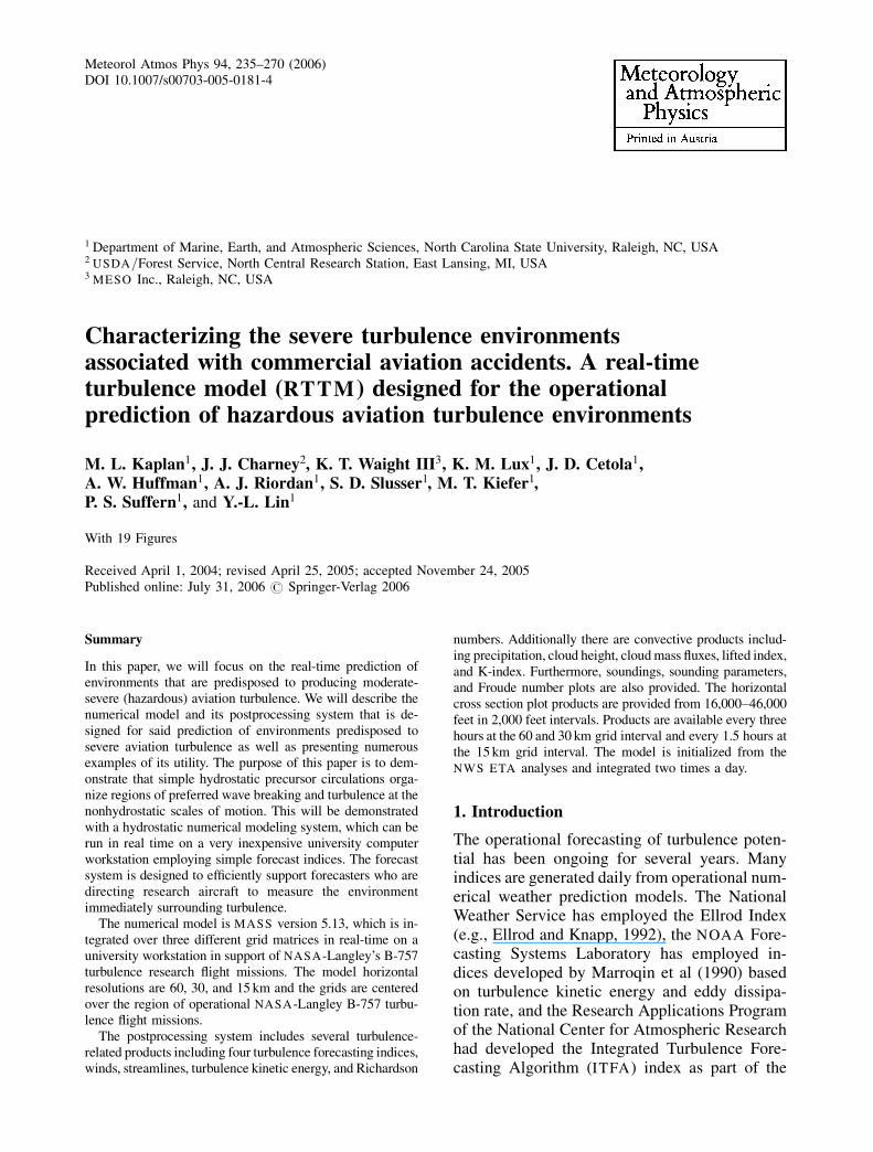
The numerical model is MASS version 5.13(Kaplan et al, 2000). The MASS model is a hy-drostatic terrain-following sigma coordinate sys-tem with comprehensive boundary layer andconvective parameterizations (note Table 1). Themodel is integrated over three different horizon-tal resolutions, i.e., 60 km, 30 km, and 15 km forthe coarse, fine1 and fine2 grids with the finesttwo meshes employing one-way nested-grid lat-eral boundary conditions (note Fig. 1). The grid

matrix size is 70� 60� 50 points for the coarsemesh grid, 90� 100� 50 points for the 30 kmgrid, and 90� 100� 50 points for the 15 kmgrid. The vertical sigma spacing is such that thereare 15 levels below 850 mb, between 850 mb and400 mb there are levels every 20 mb, and above400 mb they are spaced every 40 mb. The modelis very efficiently programmed for operationalutility. The initial state for the coarse mesh em-ploys the NWS ETA analyses at 0000 UTC and1200 UTC as well as reanalyzed rawinsonde andaviation surface observations employing an op-

Fig. 1. RTTM coarse, fine1, and fine2 gridlocations

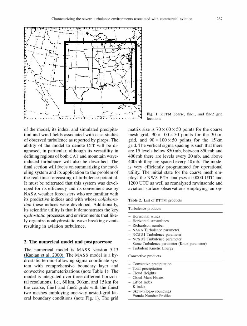
Table 2. List of RTTM products

Turbulence products

– Horizontal winds– Horizontal streamlines– Richardson number– NASA Turbulence parameter– NCSU1 Turbulence parameter– NCSU2 Turbulence parameter– Stone Turbulence parameter (Knox parameter)– Turbulent Kinetic Energy

Convective products

– Convective precipitation– Total precipitation– Cloud Heights– Cloud Mass Fluxes– Lifted Index– K-index– Skew-t=log-p soundings– Froude Number Profiles

Characterizing the severe turbulence environments associated with commercial aviation 237

timum interpolation scheme. Time-dependent lat-eral boundary conditions are derived from theNWS ETA model 40 km data set and are updatedevery 3 hours at the 60 km scale. Hourly coarsermesh simulated fields serve as the time-dependentlateral boundary conditions for the 30 and 15 kmgrid meshes. The 30 km simulation is initialized at3 hours past 0000 UTC and 1200 UTC from thecoarse mesh simulation and the 15 km simulationis initialized at 3 hours past 0300 UTC and 1500

UTC from the fine1 simulation. The three gridsare located in a manner that enables them to pro-duce simulations covering the entire 24 hour pe-riod, i.e., 24 hours at the coarse mesh, 21 hours atthe fine1 mesh, and 18 hours at the fine2 meshfrom the NWS ETA analysis data cycles consis-tent with the range of typical operational NASA-Langley B-757 turbulence research flights. Themodeling system is designed solely to supportthe NASA turbulence research flight missions.

Fig. 2a. Pireps from the NOAA

Aviation Digital Data source val-id from 1326 UTC–1508 UTC18 September 2001; (b) Watervapor infrared satellite imageryvalid at 1415 UTC 18 September2001

238 M. L. Kaplan et al

The postprocessing system is designed to sup-port real-time forecasts of turbulence potential foruse in directing the NASA B-757 research air-craft to locations of turbulence. There are fourcomponents to the postprocessor (note Table 2).The most important component is the suite ofturbulence products listed in Table 2. These

include: winds, streamlines, Richardson num-bers, turbulence kinetic energy, and four turbu-lence prediction indices. They are depicted onhorizontal surfaces from 16,000 feet to 46,000feet in 2,000 feet intervals, as mid-upper tropo-spheric turbulence is the focus of the B-757 tur-bulence research flights.

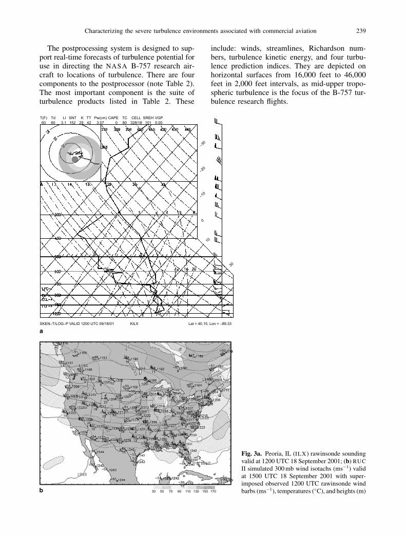
Fig. 3a. Peoria, IL (ILX) rawinsonde soundingvalid at 1200 UTC 18 September 2001; (b) RUC

II simulated 300 mb wind isotachs (ms�1) validat 1500 UTC 18 September 2001 with super-imposed observed 1200 UTC rawinsonde windbarbs (ms�1), temperatures (�C), and heights (m)

Characterizing the severe turbulence environments associated with commercial aviation 239

Fig. 4a. RTTM fine1 simulated 40,000 feetwind barbs (kts) valid at 1500 UTC 18September 2001; (b) RTTM fine1 simulated40,000 feet NCSU2 index (s-3) valid at 1500UTC 18 September 2001; (c) RTTM fine13-hour total precipitation (mm) valid from1200 UTC–1500 UTC 18 September 2001

The four indices are mathematically depictedin Eqs. (1)–(4) below.

ðV � VtÞ

0:1 þ 1000d�

dz

� �� �2; ð1Þ

V ¼wind speed; Vt ¼ 35 m=s; �¼ potential temp.if RH<95%; �¼ equivalent potential temp. ifRH� 95%

KTI ¼ f f 1 � 1

Ri

� �þ �

� �; ð2Þ

f¼Coriolis parameter; Ri¼ bulk Richardsonnumber; �¼ relative vorticity

NCSU1 ¼ ðU � rðUÞÞ jrð�ÞjjRij ; ð3Þ

U¼wind vector; Ri¼ bulk Richardson number;�¼ relative vorticity

NCSU2 ¼ jr Xr�j; ð4Þ

¼Montgomery stream function; �¼ relativevorticity.

Index no. 1 depicted in Eq. (1) is the NASA tur-bulence index developed by Proctor (2000) thatis primarily designed to determine layers of neu-tral static stability. Index no. 2 depicted in Eq. (2)

Fig. 5a. Pireps from the NOAA

Aviation Digital Data source val-id from 1631 UTC–1850 UTC16 October 2001; (b) Water va-por infrared satellite imageryvalid at 1915 UTC 16 October2001; (c) RUC II simulated500 mb temperatures (�C) validat 1800 UTC 16 October 2001with superimposed observed1200 UTC rawinsonde windbarbs (ms�1), temperatures (�C),and heights (m)

M. L. Kaplan et al: Characterizing the severe turbulence environments associated with commercial aviation 241

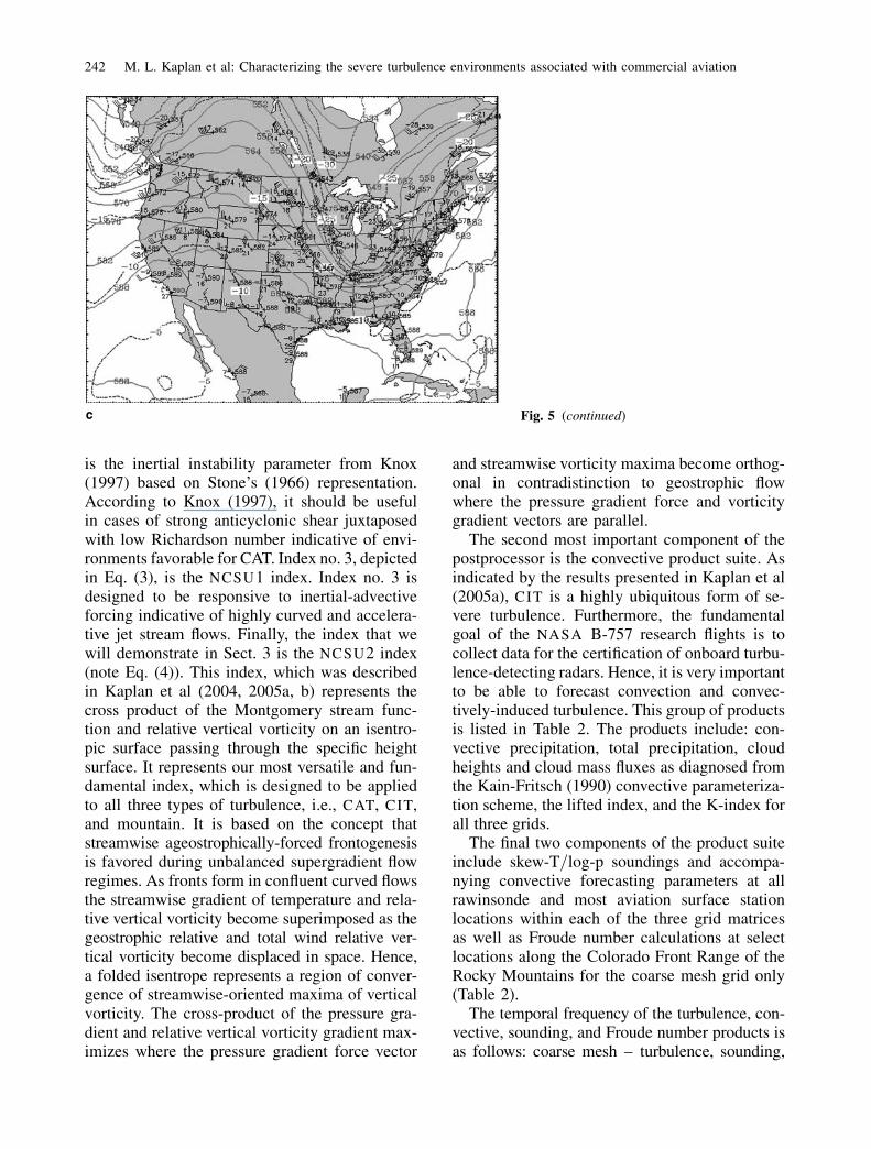
is the inertial instability parameter from Knox(1997) based on Stone’s (1966) representation.According to Knox (1997), it should be usefulin cases of strong anticyclonic shear juxtaposedwith low Richardson number indicative of envi-ronments favorable for CAT. Index no. 3, depictedin Eq. (3), is the NCSU1 index. Index no. 3 isdesigned to be responsive to inertial-advectiveforcing indicative of highly curved and accelera-tive jet stream flows. Finally, the index that wewill demonstrate in Sect. 3 is the NCSU2 index(note Eq. (4)). This index, which was describedin Kaplan et al (2004, 2005a, b) represents thecross product of the Montgomery stream func-tion and relative vertical vorticity on an isentro-pic surface passing through the specific heightsurface. It represents our most versatile and fun-damental index, which is designed to be appliedto all three types of turbulence, i.e., CAT, CIT,and mountain. It is based on the concept thatstreamwise ageostrophically-forced frontogenesisis favored during unbalanced supergradient flowregimes. As fronts form in confluent curved flowsthe streamwise gradient of temperature and rela-tive vertical vorticity become superimposed as thegeostrophic relative and total wind relative ver-tical vorticity become displaced in space. Hence,a folded isentrope represents a region of conver-gence of streamwise-oriented maxima of verticalvorticity. The cross-product of the pressure gra-dient and relative vertical vorticity gradient max-imizes where the pressure gradient force vector

and streamwise vorticity maxima become orthog-onal in contradistinction to geostrophic flowwhere the pressure gradient force and vorticitygradient vectors are parallel.

The second most important component of thepostprocessor is the convective product suite. Asindicated by the results presented in Kaplan et al(2005a), CIT is a highly ubiquitous form of se-vere turbulence. Furthermore, the fundamentalgoal of the NASA B-757 research flights is tocollect data for the certification of onboard turbu-lence-detecting radars. Hence, it is very importantto be able to forecast convection and convec-tively-induced turbulence. This group of productsis listed in Table 2. The products include: con-vective precipitation, total precipitation, cloudheights and cloud mass fluxes as diagnosed fromthe Kain-Fritsch (1990) convective parameteriza-tion scheme, the lifted index, and the K-index forall three grids.

The final two components of the product suiteinclude skew-T=log-p soundings and accompa-nying convective forecasting parameters at allrawinsonde and most aviation surface stationlocations within each of the three grid matricesas well as Froude number calculations at selectlocations along the Colorado Front Range of theRocky Mountains for the coarse mesh grid only(Table 2).

The temporal frequency of the turbulence, con-vective, sounding, and Froude number products isas follows: coarse mesh – turbulence, sounding,

Fig. 5 (continued)

242 M. L. Kaplan et al: Characterizing the severe turbulence environments associated with commercial aviation

Fig. 6a. RTTM fine1 simulated 26,000 feetwind barbs (kts) valid at 1800 UTC 16 October2001; (b) RTTM fine1 simulated 26,000feet NCSU2 index (s-3) valid at 1800 UTC16 October 2001; (c) RTTM fine1 simulated3-hour total precipitation (mm) valid from1500 UTC–1800 UTC 16 October 2001

and Froude number products at initial time andevery three hours; convective products at initialtime plus three hours and every three hours there-after, fine1 mesh – the same except starting atthree hours after 0000 UTC and 1200 UTC forturbulence and sounding products; convectiveproducts starting six hours after 0000 UTC and1200 UTC, fine2 mesh – the same for turbulenceand sounding products except starting at six hoursafter 0000 UTC and 1200 UTC and every 90 mi-nutes; convective products starting at 7.5 hoursafter 0000 UTC and 1200 UTC and every 90 mi-nutes. All horizontal plot products are available�5 hours after observed data time for the coarse

mesh, �6 hours for the fine1 mesh, and �7 hoursfor the fine2 mesh with sounding and Froudenumber products delayed �2 hours after the hor-izontal plots for each grid. The computing is per-formed on a DEC-ALPHA workstation at theDepartment of Marine, Earth, and AtmosphericSciences at North Carolina State University. Allof these products are displayed at the followingweb site: http:==shear.meas.ncsu.edu=.

3. Case study examples of RTTM simulations

In this section of the paper, we will heuristi-cally compare some of the RTTM products to

Fig. 7a. Pireps from the NOAA

Aviation Digital Data source val-id from 1126 UTC–1320 UTC5 October 2001; (b) Water vaporinfrared satellite imagery validat 1215 UTC 5 October 2001;(c) Columbus, OH (ILN) rawin-sonde sounding valid at 1200UTC 5 October 2001; (d) RUC

II simulated 200 mb wind iso-tachs (ms�1) valid at 1500 UTC5 October 2001 with super-imposed observed 1200 UTCrawinsonde wind barbs (ms�1),temperatures (�C), and heights(m)

244 M. L. Kaplan et al

the turbulence pireps as well as observations ofwinds, temperatures and clouds for several casestudies of moderate-severe turbulence. Thesecase studies were simulated in real time withthe RTTM and all products generated in real timeduring the May 2001–April 2002 time frame.Most, not all, are associated with convective pre-

cipitation and jet entrance regions consistent withthe findings in Kaplan et al (2005a, b). TheNCSU2 index fields to be displayed for thefollowing case studies range in magnitude from<1 to >200� 10�12 units of the time tendencyof enstrophy, i.e., s�3. A case study was assumedto lie in the moderate-severe range of turbu-

Fig. 7 (continued)

Characterizing the severe turbulence environments associated with commercial aviation 245

Fig. 8a. RTTM fine1 36,000 feet wind barbs(kts) valid at 1200 UTC 5 October 2001;(b) RTTM fine1 36,000 feet NCSU2 index(s-3) valid at 1200 UTC 5 October 2001;(c) RTTM fine1 simulated 3 hour precipitation(mm) valid from 0900 UTC–1200 UTC 5October 2001

lence potential if any of the following criteriaapplied:

(1) the RTTM coarse mesh values exceeded10� 10�12 units,

(2) the RTTM fine1 values exceeded 50� 10�12

units, and=or the(3) RTTM fine2 values exceeded 150� 10�12

units of the index. These thresholds werebased on daily comparisons of index maximato moderate-severe turbulence pireps. A totalof 8 moderate-severe case studies will bedescribed including 6 moderate-severe con-vective turbulence, 1 very intense day of com-bined convective and clear air sequence ofturbulence reports, and 1 moderate-severe

day of combined clear air and mountainturbulence reports. It should be emphasizedthat all of the RTTM NCSU2 turbu-lence potential index fields represent fore-casts of 6 hours or more ranging upwards of18 hours.

3.1 Convective turbulence case studies

3.1.1 Case 1 (9=18=01)

On this day, 18 September 2001, the 25,000–40,000 feet pireps, depicted in Fig. 2a, shiftabruptly southeastwards during the 1326 UTC–1508 UTC time period from the northernMississippi River Valley including Iowa and

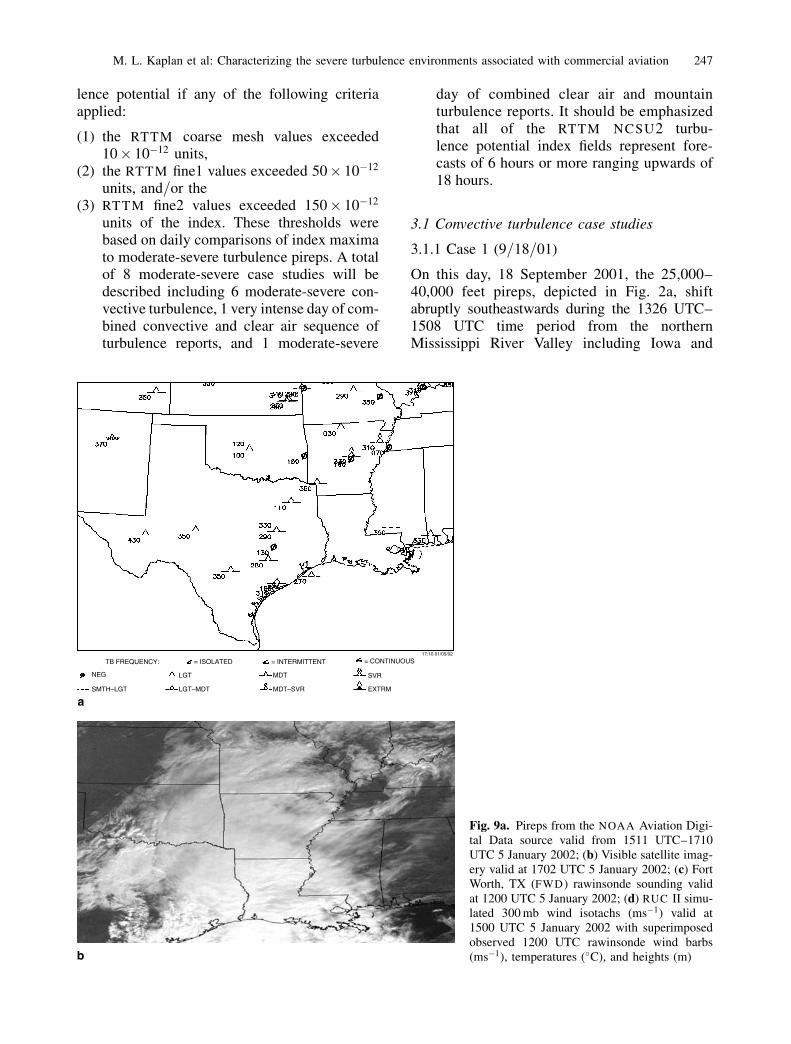
Fig. 9a. Pireps from the NOAA Aviation Digi-tal Data source valid from 1511 UTC–1710UTC 5 January 2002; (b) Visible satellite imag-ery valid at 1702 UTC 5 January 2002; (c) FortWorth, TX (FWD) rawinsonde sounding validat 1200 UTC 5 January 2002; (d) RUC II simu-lated 300 mb wind isotachs (ms�1) valid at1500 UTC 5 January 2002 with superimposedobserved 1200 UTC rawinsonde wind barbs(ms�1), temperatures (�C), and heights (m)

M. L. Kaplan et al: Characterizing the severe turbulence environments associated with commercial aviation 247

northern Missouri to southern Missouri, Illinois,and the Ohio River Valley region. A moderate-severe turbulence pilot report at 15,000 feet isapparent near St. Louis, Missouri (STL) high-lighting this southeastwards shift. The 1415 UTCwater vapor imagery in Fig. 2b indicates amassive area of convection across the northern

Mississippi River Valley and eastern sections ofKansas and Oklahoma. Apparent in this satelliteimagery are streaks of outflow oriented in ananticyclonically-curved manner across Arkansas,southern Missouri, and southern Illinois that areclose to the aforementioned rapid shift in densepirep coverage. This anticyclonic outflow and

Fig. 9 (continued)

248 M. L. Kaplan et al

relatively short-radii turning flow structure is typ-ical of a convective outflow jet-induced entranceregion (note Kaplan et al, 2005b). Observed1200 UTC soundings at Topeka, Kansas (TOP),Springfield, Missouri (SGF), and Peoria, Illinois(ILX) all indicate near neutral layers from�350 mb–250 mb with the ILX balloon (onlysounding depicted in Fig. 3a) indicating a majoranticyclonic shear zone within this near neu-tral layer. The neutral layer is indicative of adownstream cold pool aloft formed ahead ofthe lifting accompanying a convective outflowjetlet (note Kaplan et al, 2005b). Consistent withthis is the RUC-II model 1500 UTC simulated

200 mb wind fields depicted in Fig. 3b superim-posed upon the 1200 UTC rawinsonde observa-tions. This shows a classic outflow jet coveringeastern Iowa, eastern Missouri, as well as Illinoisand western Indiana and Kentucky. These fieldsstrongly suggest that the upstream convectionis producing an anticyclonically-configured out-flow jet in response to convective heating withthe strongest accelerations located well down-stream near the 2-hourly shift in turbulencepireps over eastern Missouri and southern Illinoisand Indiana.

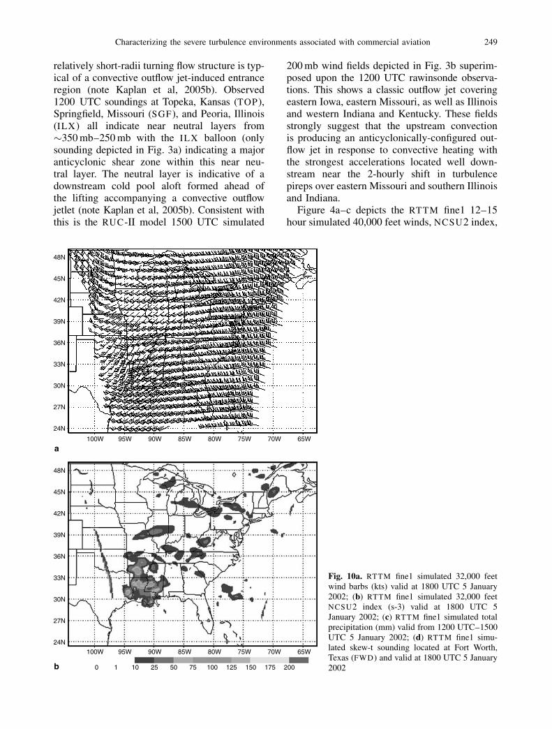
Figure 4a–c depicts the RTTM fine1 12–15hour simulated 40,000 feet winds, NCSU2 index,

Fig. 10a. RTTM fine1 simulated 32,000 feetwind barbs (kts) valid at 1800 UTC 5 January2002; (b) RTTM fine1 simulated 32,000 feetNCSU2 index (s-3) valid at 1800 UTC 5January 2002; (c) RTTM fine1 simulated totalprecipitation (mm) valid from 1200 UTC–1500UTC 5 January 2002; (d) RTTM fine1 simu-lated skew-t sounding located at Fort Worth,Texas (FWD) and valid at 1800 UTC 5 January2002

Characterizing the severe turbulence environments associated with commercial aviation 249

and total precipitation valid at 1500 UTC, 1500UTC, and from 1200 UTC–1500 UTC, respec-tively, from the 0000 UTC 18 September 2001simulation. Evident is the shift in outflow jetand index maxima ahead of the convectiveprecipitation thus forcing the maxima of theNCSU2 index >150 units of enstrophy tendencyat 40,000 feet from central Missouri southeast-

wards into Illinois. This NCSU2 index maximalocation is more consistent with the pirepsdepicted in Fig. 2a. The NCSU2 index at36,000 and 30,000 feet is very similar to the40,000 feet values (not shown) indicating thatthe layer from just below 300 mb to just above200 mb was accelerating under the influence ofconvective heating upstream and that the convec-

Fig. 10 (continued)

250 M. L. Kaplan et al

tively-accelerated entrance region over Missouriwas close to the index maxima and thereforelikely contributing to the favorable environmentfor turbulence. This is consistent with the infer-ences drawn from the satellite and rawinsondeobservations.

3.1.2 Case 2 (10=16=01)

Pilot reports from 1631 UTC–1850 UTC indi-cate several moderate to severe turbulence en-counters over southwestern Pennsylvania andwestern Maryland between 15,000 and 27,000

feet (Fig. 5a). The water vapor satellite imageryindicated a sharp comma cloud with convec-tion over westcentral Pennsylvania at 1915 UTC(Fig. 5b). The turbulence maximum is close to thestrong 500 mb front as noted in the RUC analysesin Fig. 5c.

The RTTM fine1 six-hour simulated 26,000feet NCSU2 index as well as winds and total pre-cipitation for the period from 1500 UTC–1800UTC are depicted in Fig. 6a–c. The NCSU2 indexshows a comma-shaped maxima and bulls eye>150 units over southwestern Pennsylvania andprecipitation is simulated to fall just upstream

Fig. 11a. Pireps from theNOAA Aviation Digital Datasource valid from 1028 UTC–1157 UTC 11 October 2001;(b) Water vapor infrared satel-lite imagery valid at 1145 UTC11 October 2001; (c) Columbus,Ohio (ILN) rawinsonde sound-ing valid at 1200 UTC 11October 2001; (d) RUC IIsimulated 200 mb wind isotachs(ms�1) valid at 0900 UTC 11October 2001 with superimposedobserved 0000 UTC rawinsondewind barbs (ms�1), temperatures(�C), and heights (m)

Characterizing the severe turbulence environments associated with commercial aviation 251

near Pittsburgh (PIT) indicating that the maxi-mum index values were just downstream fromthe convection. The 1500 UTC–1800 UTC con-vection in the RTTM shifts the 1800 UTCNCSU2 index maximum slightly downstreamfrom the 500 mb front in Fig. 5c thus reflecting

the effect of convective forcing. Additionally thesimulated sounding at Buffalo, NY (BUF) (notshown) indicates a strong signal of the neutrallayer and vertical shear maximum near the26,000 feet level in proximity to the height of theobserved turbulence. However, it is fair to say that

Fig. 11 (continued)

252 M. L. Kaplan et al

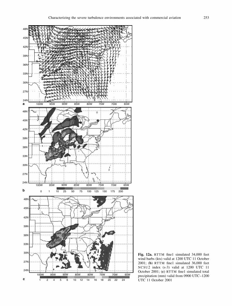
Fig. 12a. RTTM fine1 simulated 34,000 feetwind barbs (kts) valid at 1200 UTC 11 October2001; (b) RTTM fine1 simulated 36,000 feetNCSU2 index (s-3) valid at 1200 UTC 11October 2001; (c) RTTM fine1 simulated totalprecipitation (mm) valid from 0900 UTC–1200UTC 11 October 2001

Characterizing the severe turbulence environments associated with commercial aviation 253

Fig. 13a. Pireps from the NOAA AviationDigital Data source valid from 1650–1843UTC 17 February 2002; (b) Infrared satelliteimagery valid at 1846 UTC 17 February 2002;(c) RUC II simulated 500 mb temperatures(�C) valid at 1800 UTC 17 February 2002with superimposed observed 1200 UTC rawin-sonde wind barbs (ms�1), temperatures (�C),and heights (m)

254 M. L. Kaplan et al

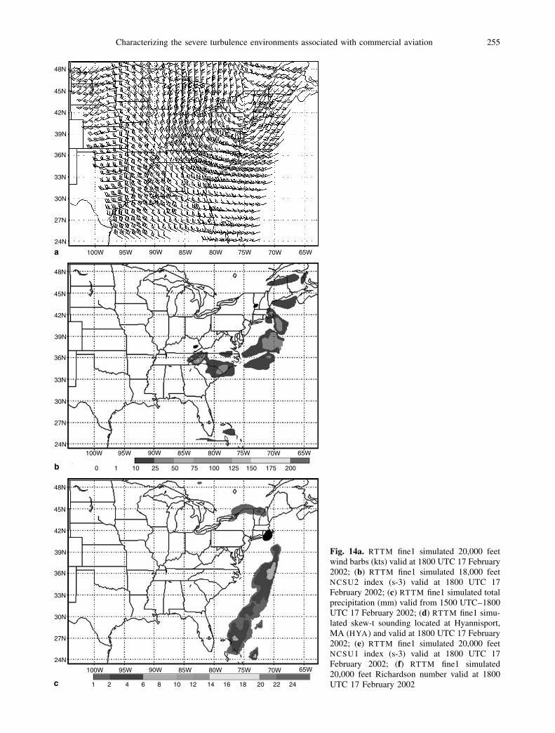
Fig. 14a. RTTM fine1 simulated 20,000 feetwind barbs (kts) valid at 1800 UTC 17 February2002; (b) RTTM fine1 simulated 18,000 feetNCSU2 index (s-3) valid at 1800 UTC 17February 2002; (c) RTTM fine1 simulated totalprecipitation (mm) valid from 1500 UTC–1800UTC 17 February 2002; (d) RTTM fine1 simu-lated skew-t sounding located at Hyannisport,MA (HYA) and valid at 1800 UTC 17 February2002; (e) RTTM fine1 simulated 20,000 feetNCSU1 index (s-3) valid at 1800 UTC 17February 2002; (f) RTTM fine1 simulated20,000 feet Richardson number valid at 1800UTC 17 February 2002

Characterizing the severe turbulence environments associated with commercial aviation 255

the strong 500 mb front allows the NCSU2 indexmaxima to be relatively closely juxtaposed to themidtropospheric baroclinic zone unlike the pre-vious case study where the NCSU2 index max-ima was more substantially detached from thebackground jet=front system and more closely

coupled to the convective maxima,, i.e., the back-ground confluence maximum within the jet=frontsystem is just as important for substantial indexvalues in the RTTM indicating the significant roleof adiabatic forcing in organizing an environ-ment predisposed to turbulence in this case study.

Fig. 14 (continued)

256 M. L. Kaplan et al

3.1.3 Case 3 (10=5=01)

This case study strongly suggests major differencesfrom the previous case study in that the RTTM

index maxima are based on the development ofa convective outflow jet not unlike case study 1,in particular. The turbulence pireps during the1126 UTC–1320 UTC time frame depicted inFig. 7a indicate a swath of almost unbrokenmoderate intensity activity from Kansas throughMissouri, Illinois, Indiana, and Ohio. This beltof observed turbulence is nearly coincident withthe split structure in the convection in the 1215UTC water vapor imagery depicted in Fig. 7band is closely aligned, actually just northwest of,the anticyclonic turning flow in the rawinsondesat 1200 UTC superimposed on the 1500 UTCRUC 200 mb winds in Fig. 7d. Soundings atPeoria, Illinois (ILX) and Columbus, Ohio (ILN)at 0000 UTC and 1200 UTC, respectively indi-cated a deep neutral layer above 350 mb (ILN

sounding is depicted in Fig. 7c). Hence, there issome proof supporting a convectively-enhancedjet which acts to split the flow and produce con-ditions not unlike that shown in case study 1,above.

The 36,000 feet winds and NCSU2 index at1200 UTC 10=5=01 as well as 3 hour precipita-tion valid at 1200 UTC from the 0000 UTC10=5=01 RTTM fine1 simulation depicted inFig. 8a–c nicely show how the RTTM is devel-oping a separate convectively-enhanced anti-

cyclonic outflow jet from Missouri to northernOhio. This outflow jet lies south of the main(large scale) jet entrance region producing aswath of high turbulence probability >150 unitsnear the observed turbulence. The heavy con-vective precipitation simulated to occur overMissouri accelerates the flow downstream overnorthern Illinois, Indiana, and Ohio providingthe vorticity gradients necessary to trigger largeindex values south of the large scale jet entranceregion.

3.1.4 Case 4 (1=5=02)

This case study represents yet another example ofsevere convective turbulence. Figure 9a depictsthe turbulence pireps between 1511 UTC and1710 UTC. An examination of these fields indi-cates that several moderate to severe reports occurearly in the day over central and northeasternArkansas with a shift in the moderate activityabruptly towards the lower Ohio River Valleyregion later in the day (not shown). Additionally,the airmets (not shown) do not anticipate turbu-lence in the region where it occurs, i.e., focusingthe strongest warning area south of the Louisianacoastal region.

Visible satellite imagery valid at 1702 UTC, therawinsonde sounding at Fort Worth, Texas (FWD)valid at 1200 UTC, and the RUC 300 mb anal-yses valid at 1500 UTC in Fig. 9b, c, and d allstrongly indicate a subsynoptic jet streak that is,

Fig. 14 (continued)

Characterizing the severe turbulence environments associated with commercial aviation 257

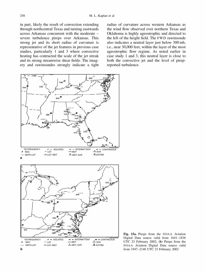
in part, likely the result of convection extendingthrough northcentral Texas and turning eastwardsacross Arkansas concurrent with the moderate –severe turbulence pireps over Arkansas. Thisstrong jet and its short radius of curvature isrepresentative of the jet features in previous casestudies, particularly 1 and 3 where convectiveheating has contracted the scale of the jet streakand its strong streamwise shear fields. The imag-ery and rawinsondes strongly indicate a tight

radius of curvature across western Arkansas asthe wind flow observed over northern Texas andOklahoma is highly ageostrophic and directed tothe left of the height field. The FWD rawinsondealso indicates a neutral layer just below 300 mb,i.e., near 30,000 feet, within the layer of the mostageostrophic flow regime. As noted earlier incase study 1 and 3, this neutral layer is close toboth the convective jet and the level of pirep-reported turbulence.

Fig. 15a. Pireps from the NOAA AviationDigital Data source valid from 1641–1836UTC 23 February 2002; (b) Pireps from theNOAA Aviation Digital Data source validfrom 1947–2140 UTC 23 February 2002

258 M. L. Kaplan et al

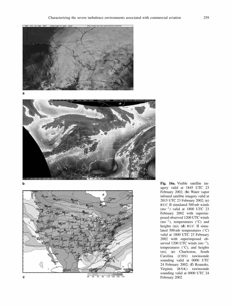
Fig. 16a. Visible satellite im-agery valid at 1845 UTC 23February 2002; (b) Water vaporinfrared satellite imagery valid at2015 UTC 23 February 2002; (c)RUC II simulated 300 mb winds(ms�1) valid at 1800 UTC 23February 2002 with superim-posed observed 1200 UTC winds(ms�1), temperatures (�C) andheights (m); (d) RUC II simu-lated 500 mb temperatures (�C)valid at 1800 UTC 23 February2002 with superimposed ob-served 1200 UTC winds (ms�1),temperatures (�C), and heights(m); (e) Charleston, SouthCarolina (CHS) rawinsondesounding valid at 0000 UTC24 February 2002; (f) Roanoke,Virginia (RNK) rawinsondesounding valid at 0000 UTC 24February 2002

Characterizing the severe turbulence environments associated with commercial aviation 259

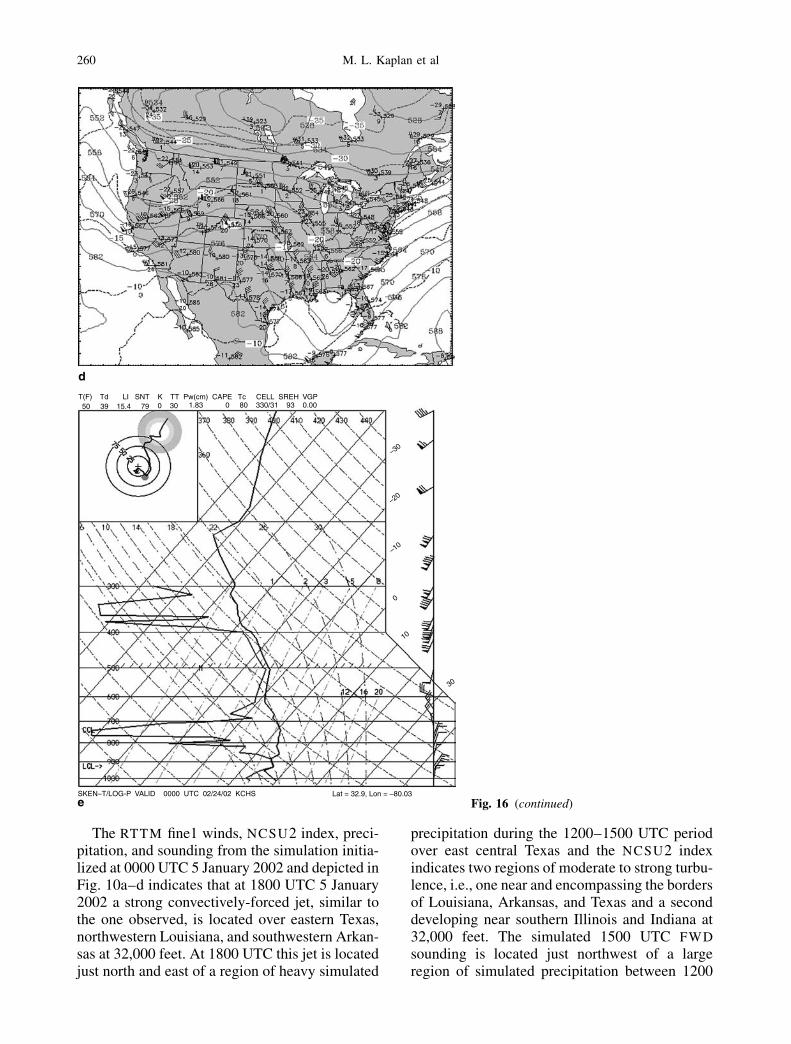
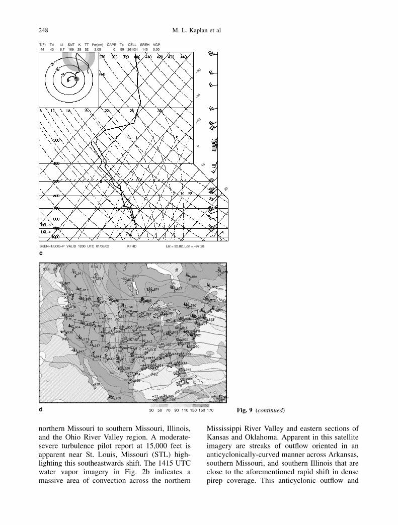
The RTTM fine1 winds, NCSU2 index, preci-pitation, and sounding from the simulation initia-lized at 0000 UTC 5 January 2002 and depicted inFig. 10a–d indicates that at 1800 UTC 5 January2002 a strong convectively-forced jet, similar tothe one observed, is located over eastern Texas,northwestern Louisiana, and southwestern Arkan-sas at 32,000 feet. At 1800 UTC this jet is locatedjust north and east of a region of heavy simulated

precipitation during the 1200–1500 UTC periodover east central Texas and the NCSU2 indexindicates two regions of moderate to strong turbu-lence, i.e., one near and encompassing the bordersof Louisiana, Arkansas, and Texas and a seconddeveloping near southern Illinois and Indiana at32,000 feet. The simulated 1500 UTC FWD

sounding is located just northwest of a largeregion of simulated precipitation between 1200

Fig. 16 (continued)

260 M. L. Kaplan et al

UTC and 1500 UTC. It is interesting that the 1500UTC FWD simulated sounding captures some ofthe observed deep neutral layer structure, i.e.,below 500 mb, as well as the strong vertical varia-tion of wind velocity and directional shear in par-ticular, from southwest to south back to southwestin the vertical near the level of observed shear at1200 UTC. The RTTM fine1 simulated fieldsinitialized at 0000 UTC 5 January 2002 indicatethe tendency towards a shift of the turbulence po-tential >150 units from Louisiana and Arkansasat 1800 UTC to over the lower Ohio River Valleyby 2100 UTC (not shown) analogous to the newlydeveloping pireps over this region (not shown) aswell as the growth of the convectively-forced jetnortheastwards. Hence, the RTTM favors highestturbulence potential over Louisiana and Arkansaswith a jump in the maxima similar to where it isobserved to occur.

3.1.5 Case 5 (10=11=01)

This case study is very similar to case studies 1,3, and 4 in terms of strong convective outflowjet formation. During the early morning hours of

11 October 2001 the focus of pireps shifts east-wards into the Ohio River Valley from the over-night maxima in the eastern Great Plains andMississippi River Valley. Figure 11a depictsthese pireps from 1028–1157 UTC. Water vaporsatellite imagery at �1145 UTC, the observedsounding at Columbus, Ohio (ILN) valid at 1200UTC, and 200 mb RUC analyses winds validat 0900 UTC with superimposed 0000 UTC10=11=01 rawinsondes depicted in Fig. 11b, c,and d all are similar to a pattern seen in casestudies 1, 3, and 4. Convection in the lower Mis-sissippi River Valley amplifies a jet streak overthe upper Missisippi River Valley and westernOhio River Valley during the overnight period.This results in a split anticyclonic structure tothe downstream water vapor imagery accompa-nying a secondary anticyclonic wind maximumover Indiana by 1100 UTC. The 1200 UTC raw-insonde at ILN has a strong anticyclonic shearforced by the strong westerly component in-crease with height in the upper troposphere be-tween 300 mb and 250 mb with near neutrallayers just below the region of strongest anti-cyclonic shear.

Fig. 16 (continued)

Characterizing the severe turbulence environments associated with commercial aviation 261

Fig. 17a. RTTM fine1 simulated 22,000 feetwind barbs (kts) valid at 2100 UTC 23February 2002; (b) RTTM fine1 simulated22,000 feet NCSU2 index (s-3) valid at 1800UTC 23 February 2002; (c) RTTM fine1 simu-lated 24,000 feet NCSU2 index (s-3) valid at2100 UTC 23 February 2002; (d) RTTM fine1simulated total precipitation (mm) valid from1500 UTC–1800 UTC 23 February 2002; (e)RTTM fine1 simulated 22,000 feet Richardsonnumber valid at 2100 UTC 23 February 2002;(f) RTTM fine1 simulated skew-t sounding lo-cated at Charleston, South Carolina (CHS) andvalid at 0000 UTC 24 February 2002

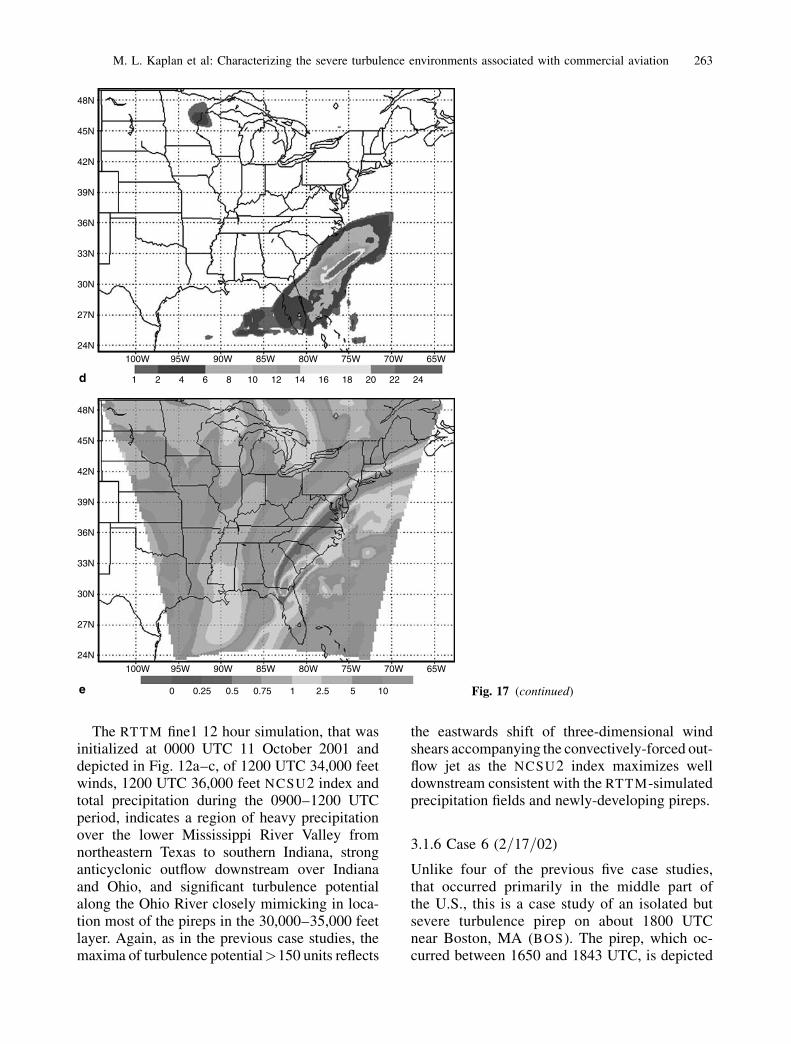
The RTTM fine1 12 hour simulation, that wasinitialized at 0000 UTC 11 October 2001 anddepicted in Fig. 12a–c, of 1200 UTC 34,000 feetwinds, 1200 UTC 36,000 feet NCSU2 index andtotal precipitation during the 0900–1200 UTCperiod, indicates a region of heavy precipitationover the lower Mississippi River Valley fromnortheastern Texas to southern Indiana, stronganticyclonic outflow downstream over Indianaand Ohio, and significant turbulence potentialalong the Ohio River closely mimicking in loca-tion most of the pireps in the 30,000–35,000 feetlayer. Again, as in the previous case studies, themaxima of turbulence potential>150 units reflects

the eastwards shift of three-dimensional windshears accompanying the convectively-forced out-flow jet as the NCSU2 index maximizes welldownstream consistent with the RTTM-simulatedprecipitation fields and newly-developing pireps.

3.1.6 Case 6 (2=17=02)

Unlike four of the previous five case studies,that occurred primarily in the middle part ofthe U.S., this is a case study of an isolated butsevere turbulence pirep on about 1800 UTCnear Boston, MA (BOS). The pirep, which oc-curred between 1650 and 1843 UTC, is depicted

Fig. 17 (continued)

M. L. Kaplan et al: Characterizing the severe turbulence environments associated with commercial aviation 263

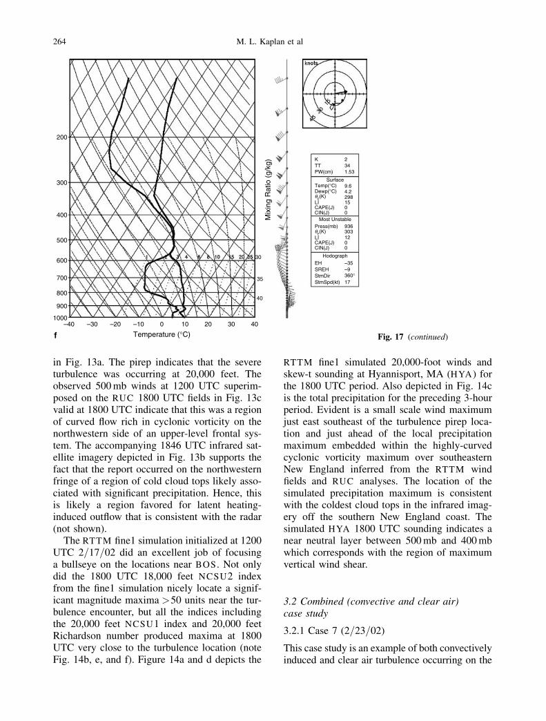
in Fig. 13a. The pirep indicates that the severeturbulence was occurring at 20,000 feet. Theobserved 500 mb winds at 1200 UTC superim-posed on the RUC 1800 UTC fields in Fig. 13cvalid at 1800 UTC indicate that this was a regionof curved flow rich in cyclonic vorticity on thenorthwestern side of an upper-level frontal sys-tem. The accompanying 1846 UTC infrared sat-ellite imagery depicted in Fig. 13b supports thefact that the report occurred on the northwesternfringe of a region of cold cloud tops likely asso-ciated with significant precipitation. Hence, thisis likely a region favored for latent heating-induced outflow that is consistent with the radar(not shown).

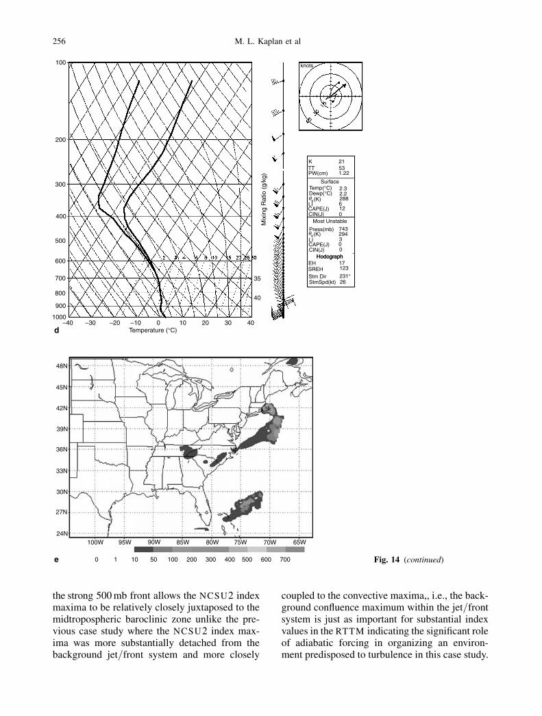
The RTTM fine1 simulation initialized at 1200UTC 2=17=02 did an excellent job of focusinga bullseye on the locations near BOS. Not onlydid the 1800 UTC 18,000 feet NCSU2 indexfrom the fine1 simulation nicely locate a signif-icant magnitude maxima >50 units near the tur-bulence encounter, but all the indices includingthe 20,000 feet NCSU1 index and 20,000 feetRichardson number produced maxima at 1800UTC very close to the turbulence location (noteFig. 14b, e, and f). Figure 14a and d depicts the

RTTM fine1 simulated 20,000-foot winds andskew-t sounding at Hyannisport, MA (HYA) forthe 1800 UTC period. Also depicted in Fig. 14cis the total precipitation for the preceding 3-hourperiod. Evident is a small scale wind maximumjust east southeast of the turbulence pirep loca-tion and just ahead of the local precipitationmaximum embedded within the highly-curvedcyclonic vorticity maximum over southeasternNew England inferred from the RTTM windfields and RUC analyses. The location of thesimulated precipitation maximum is consistentwith the coldest cloud tops in the infrared imag-ery off the southern New England coast. Thesimulated HYA 1800 UTC sounding indicates anear neutral layer between 500 mb and 400 mbwhich corresponds with the region of maximumvertical wind shear.

3.2 Combined (convective and clear air)case study

3.2.1 Case 7 (2=23=02)

This case study is an example of both convectivelyinduced and clear air turbulence occurring on the

Fig. 17 (continued)

264 M. L. Kaplan et al

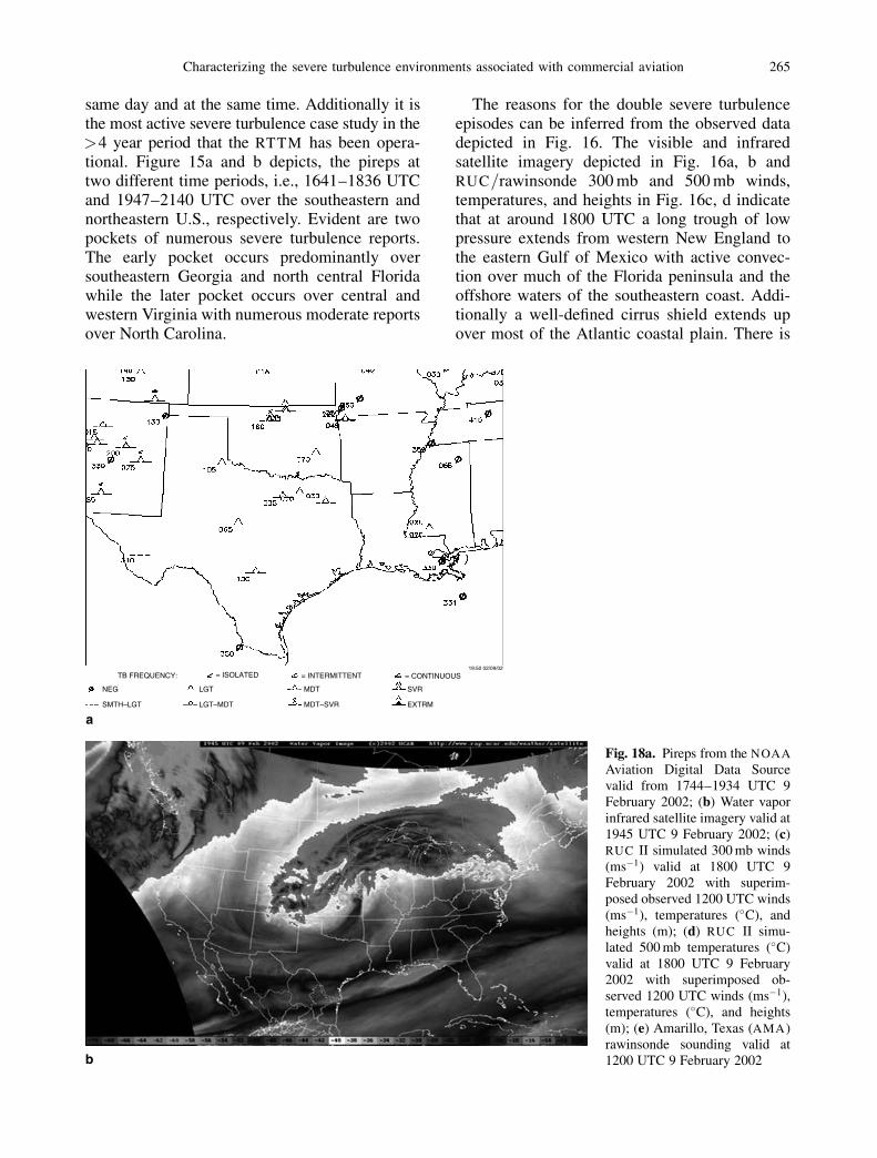
same day and at the same time. Additionally it isthe most active severe turbulence case study in the>4 year period that the RTTM has been opera-tional. Figure 15a and b depicts, the pireps attwo different time periods, i.e., 1641–1836 UTCand 1947–2140 UTC over the southeastern andnortheastern U.S., respectively. Evident are twopockets of numerous severe turbulence reports.The early pocket occurs predominantly oversoutheastern Georgia and north central Floridawhile the later pocket occurs over central andwestern Virginia with numerous moderate reportsover North Carolina.

The reasons for the double severe turbulenceepisodes can be inferred from the observed datadepicted in Fig. 16. The visible and infraredsatellite imagery depicted in Fig. 16a, b andRUC=rawinsonde 300 mb and 500 mb winds,temperatures, and heights in Fig. 16c, d indicatethat at around 1800 UTC a long trough of lowpressure extends from western New England tothe eastern Gulf of Mexico with active convec-tion over much of the Florida peninsula and theoffshore waters of the southeastern coast. Addi-tionally a well-defined cirrus shield extends upover most of the Atlantic coastal plain. There is

Fig. 18a. Pireps from the NOAA

Aviation Digital Data Sourcevalid from 1744–1934 UTC 9February 2002; (b) Water vaporinfrared satellite imagery valid at1945 UTC 9 February 2002; (c)RUC II simulated 300 mb winds(ms�1) valid at 1800 UTC 9February 2002 with superim-posed observed 1200 UTC winds(ms�1), temperatures (�C), andheights (m); (d) RUC II simu-lated 500 mb temperatures (�C)valid at 1800 UTC 9 February2002 with superimposed ob-served 1200 UTC winds (ms�1),temperatures (�C), and heights(m); (e) Amarillo, Texas (AMA)rawinsonde sounding valid at1200 UTC 9 February 2002

Characterizing the severe turbulence environments associated with commercial aviation 265

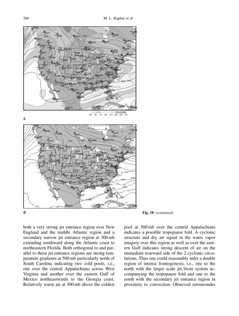
both a very strong jet entrance region over NewEngland and the middle Atlantic region and asecondary narrow jet entrance region at 300 mbextending southward along the Atlantic coast tonortheastern Florida. Both orthogonal to and par-allel to these jet entrance regions are strong tem-perature gradients at 500 mb particularly north ofSouth Carolina indicating two cold pools, i.e.,one over the central Appalachians across WestVirginia and another over the eastern Gulf ofMexico northeastwards to the Georgia coast.Relatively warm air at 300 mb above the coldest

pool at 500 mb over the central Appalachiansindicates a possible tropopause fold. A cyclonicstructure and dry air signal in the water vaporimagery over this region as well as over the east-ern Gulf indicates strong descent of air on theimmediate rearward side of the 2 cyclonic circu-lations. Thus one could reasonably infer a doubleregion of intense frontogenesis, i.e., one to thenorth with the larger scale jet=front system ac-companying the tropopause fold and one to thesouth with the secondary jet entrance region inproximity to convection. Observed rawinsondes

Fig. 18 (continued)

266 M. L. Kaplan et al

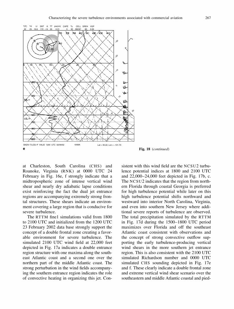
at Charleston, South Carolina (CHS) andRoanoke, Virginia (RNK) at 0000 UTC 24February in Fig. 16e, f strongly indicate that amidtropospheric zone of intense vertical windshear and nearly dry adiabatic lapse conditionsexist reinforcing the fact the dual jet entranceregions are accompanying extremely strong fron-tal structures. These shears indicate an environ-ment covering a large region that is conducive forsevere turbulence.

The RTTM fine1 simulations valid from 1800to 2100 UTC and initialized from the 1200 UTC23 February 2002 data base strongly support theconcept of a double frontal zone creating a favor-able environment for severe turbulence. Thesimulated 2100 UTC wind field at 22,000 feetdepicted in Fig. 17a indicates a double entranceregion structure with one maxima along the south-east Atlantic coast and a second one over thenorthern part of the middle Atlantic coast. Thestrong perturbation in the wind fields accompany-ing the southern entrance region indicates the roleof convective heating in organizing this jet. Con-

sistent with this wind field are the NCSU2 turbu-lence potential indices at 1800 and 2100 UTCand 22,000–24,000 feet depicted in Fig. 17b, c.The NCSU2 indicates that the region from north-ern Florida through coastal Georgia is preferredfor high turbulence potential while later on thishigh turbulence potential shifts northward andwestward into interior North Carolina, Virginia,and even into southern New Jersey where addi-tional severe reports of turbulence are observed.The total precipitation simulated by the RTTM

in Fig. 17d during the 1500–1800 UTC periodmaximizes over Florida and off the southeastAtlantic coast consistent with observations andthe concept of strong convective outflow sup-porting the early turbulence-producing verticalwind shears in the more southern jet entranceregion. This is also consistent with the 2100 UTCsimulated Richardson number and 0000 UTCsimulated CHS sounding depicted in Fig. 17eand f. These clearly indicate a double frontal zoneand extreme vertical wind shear scenario over thesoutheastern and middle Atlantic coastal and pied-

Fig. 18 (continued)

Characterizing the severe turbulence environments associated with commercial aviation 267

mont regions consistent with the observations ofatmospheric variables and severe turbulence.

3.3 Combined (clear air and mountain)case study

3.3.1 Case 8 (2=9=02)

In contradistinction to the preceding case studies,this was a clear air turbulence case and mountainturbulence case with little or no moist convection,i.e., in many ways a classic example of a tropo-pause fold case study. Figure 18c and d depictsthe RUC analysis 500 mb and 300 mb wind andtemperature fields which indicated that a highlycurved jet streak entrance region and very strongfrontal system was approaching the region of ob-served severe turbulence (north-central Oklahoma)reported in the pireps depicted in Fig. 18a shortly

before 1900 UTC. Also, a second maxima inthe jet stream was rotating across eastern Utahnear additional severe pireps over New Mexicoand Colorado. The Amarillo, Texas (AMA) 1200UTC observed sounding in Fig. 18e indicated adry adiabatic layer at the same level of the se-vere turbulence report, i.e., 23,000 feet, and thewater vapor infrared satellite imagery depicted inFig. 18b confirmed the absence of deep convec-tion and very highly curved and sheared flowover northern Texas and northwestern Oklahomaat 1900 UTC. In spite of these strong signals ofthree-dimensional shear and frontal structure, theairmets (not shown) do not highlight this regionover Oklahoma as the most favored for verystrong turbulence, i.e., the focus is farther west-ward in the mountainous regions.

The 1800 UTC RTTM coarse NCSU2 indexvalues initialized at 1200 UTC 9 February 2002

Fig. 19a. RTTM Coarse simulated 22,000feet wind barbs (kts) valid at 1800 UTC 9February 2002; (b) RTTM Coarse simulated22,000 feet NCSU2 index valid at 1800 UTC9 February 2002; (c) RTTM Coarse simulatedskew-t sounding located at Oklahoma City,Oklahoma (OKC) and valid at 1800 UTC 9February 2002

268 M. L. Kaplan et al

and depicted in Fig. 19b unambiguously depictmaxima over north-central Oklahoma and themountains of the intermountain west. The RTTM

coarse NCSU2 index recorded the highest indexvalue for the coarse mesh simulation of any ofthese case studies by exceeding 50 units. Thesimulated winds in Fig. 19a show the significantcurvature and horizontal shear from which onecan infer the strong gradients of vertical vorticityas well as the low Richardson numbers inferredfrom the vertical wind shear and neutral layer inthe observed Amarillo, Texas (AMA) soundingdepicted in Fig. 18e and simulated OklahomaCity, Oklahoma (OKC) sounding depicted inFig. 19c. This case study indicates that the RTTM

has the potential to diagnose nonconvective tur-bulence as accurately as convective turbulence.

4. Conclusions

A real-time turbulence model and its postpro-cessing system are described and several examplesof its use in predicting the organizing environmentfor moderate and severe turbulence are presented.The system is designed for efficiency in supportof an operational flight experiment. The doubly

nested-grid modeling system is designed to pre-dict the potential for atmospheric turbulence inclear air, convection, and in proximity to moun-tains. The system produces 4 turbulence indices,numerous convective products, winds, streamlines,Richardson numbers, soundings, and Froude num-ber calculations at 60, 30, and 15 km horizontalresolutions and 2000 foot vertical resolutions overmuch of the continental U.S. in support of theNASA-Langley B-757 operational turbulence re-search flights. It is the efficiency and tailoring ofthe system and its products that enabled NASA

weather forecasters to employ this in a manner,which meets their technical requirements.

Several case studies of observed moderate –severe turbulence are described wherein 6–18hour forecasts of turbulence potential from theRTTM NCSU2 index are compared to pirepsand observations. The RTTM NCSU2 index iscompared to observed winds, temperatures, andsatellite imagery in an effort to heuristically diag-nose its utility as a forecasting tool. The simplic-ity of the index enables scientific evaluation ofits utility to be straightforward and tractableunlike many more complex and intricate forecastindices. Select case study analyses indicate that

Fig. 19 (continued)

Characterizing the severe turbulence environments associated with commercial aviation 269

the RTTM index tends to perform well in theprediction of regions of both convective and clearair turbulence potential 6–18 hours prior to anobserved report of an aircraft’s encounter withmoderate – severe turbulence. The scientific im-plication here is that certain modes of hydrostaticforcing, often involving anticyclonically curvedand accelerating convective outflow jetlets aswell as their accompanying streamwise mesos-cale frontal zones, may be very important inorganizing the fine scale nonhydrostatic scalesof motion for turbulence, which is consistentwith the findings of Kaplan et al (2005b). Theseresults are for select individual case study com-parisons, however, and are not as rigorously con-vincing of the utility of the RTTM as an in depthstatistical evaluation of a large number of casestudies. Such an evaluation is being performedat the present time.

Acknowledgements

This research has been funded under the Turbulence Predic-tion and Warning System element of NASA’ Aviation SafetyProgram under NASA contract no. NASA1-02007. Theauthors wish to acknowledge the support of Dr. Fred H.Proctor, the NASA-Langley Technical Contract Monitor.Figures employed in this paper were extracted from NASA=CR-2004-213025. Support was also provided by AFRL con-tract no. FA8718-04-C-0011.

References

Ellrod GP, Knapp DI (1992) An objective clear air turbu-lence forecasting technique: verification and operationaluse. Wea Forecast 7: 150–165

Kain JS, Fritsch JM (1990) A one-dimensional entraining-detraining plume model. J Atmos Sci 47: 2784–2802

Kaplan ML, Lin Y-L, Charney JJ, Pfeiffer KD, Ensley DB,DeCroix DS, Weglarz RP (2000) A terminal area PBL

prediction system at Dallas–Fort Worth and its applica-tion in simulating diurnal PBL jets. Bull Amer Meteor Soc81: 2179–2204

Kaplan ML, Lux KM, Cetola JD, Huffman AW, Riordan AJ,Slusser SW, Lin YL, Charney JJ, Waight KT III (2004)Characterizing the severe turbulence environments as-sociated with commercial aviation accidents. A Real-Time Turbulence Model (RTTM) designed for theoperational prediction of hazardous aviation turbulenceenvironments. NASA/CR-2004-213025, NASA LangleyResearch Center, August 2004, 54 pp

Kaplan ML, Huffman AW, Lux KM, Cetola JD, Charney JJ,Riordan AJ, Lin Y-L, Waight KT III (2005a) Charac-terizing the severe turbulence environments associatedwith commercial aviation accidents. A 44-case studysynoptic observational analyses. Meteorol Atmos Phys88: 129–152

Kaplan ML, Huffman AW, Lux KM, Cetola JD, Charney JJ,Riordan AJ, Lin Y-L, Waight KT III (2005b) Charac-terizing the severe turbulence environments associatedwith commercial aviation accidents. Hydrostatic meso-scale numerical simulations of supergradient wind flowand ageostrophic along-stream frontogenesis. MeteorolAtmos Phys 88: 153–173

Knox JA (1997) Possible mechanisms of clear air turbu-lence in strongly anticyclonic flows. Mon Wea Rev 125:1251–1259

Marroquin A (1998) An advanced algorithm to diagnoseatmospheric turbulence using numerical model output.Preprints, 16th Conf. on Weather Analysis and Fore-casting, 11–16 January, 1998 Phoenix, AZ, pp 79–81

Proctor FH (2000) Personal communicationSharman R, Wiener G, Brown B (2000) Description and

verification of the NCAR Integrated Turbulence Fore-casting Algorithm (ITFA). AIAA 00-0493. AIAA 38thAerospace Sciences Meeting and Exhibit, 10–13 January,2000-AIAA, Reno, NV

Stone PH (1966) On non-geostrophic baroclinic instability.J Atmos Sci 23: 390–400

Corresponding author’s address: Yuh-Lang Lin, Depart-ment of Marine, Earth, and Atmospheric Sciences, Box8208, North Carolina State University, Raleigh, NorthCarolina 27695-8208, USA (E-mail: [email protected])

Verleger: Springer-Verlag GmbH, Sachsenplatz 4–6, 1201 Wien, Austria. – Herausgeber: Prof. Dr. Reinhold Steinacker, Institut fur Meteorologie und Geophysik,Universitat Wien, Althanstraße 14, 1090 Wien, Austria. – Redaktion: Althanstraße 14, 1090 Wien, Austria. – Satz und Umbruch: Thomson Press (India) Ltd., Chennai. –

Druck und Bindung: Grasl Druck&Neue Medien, 2540 Bad Voslau, Austria. – Verlagsort: Wien. – Herstellungsort: Bad Voslau. – Printed in Austria.

270 M. L. Kaplan et al: Characterizing the severe turbulence environments associated with commercial aviation