Characterization of transversal electrophoresis based microflow devices for water purification

"Sapienza" University of Rome

Faculty of Engineering

Thesis submitted in partial fulfillment of the requirements for the

Master’s degree in Nanotechnology Engineering

Characterization of transversalelectrophoresis based microflow devices

for water purification

Student Academic Supervisor

Enrico Brinciotti Prof. C.M. Casciola

Industrial Supervisor

Ir. Alwin Verschueren

a.a. 2011/2012

I would like to dedicate this thesis to my loving parents, to mybrother Luca, and to my girlfriend Michela; for their endless love,support and encouragement throughout different periods of my life.

"There are the rushing waves...mountains of molecules,

each stupidly minding its own business...trillions apart

...yet forming white surf in unison.Here it is standing: atoms with consciousness; matter with curiosity.

Stands at the sea, wondering: I...a universe of atomsan atom in the universe."

Richard Feynman

Acknowledgements

I would like to express my sincere gratitude to Ir. Alwin Verschueren,my supervisor at Philips Research, for providing me the opportunityto do my final project work at Philips. His patient guidance, en-thusiastic encouragement and useful critiques have been very muchappreciated.I acknowledge Philips for the housing and laboratory facilities. The8 months experience has been unquestionably enriching.My grateful thanks are also extended to Prof. C. M. Casciola, myacademic supervisor at Sapienza University of Rome. Without hisvaluable course and education it would not have been possible to facethis experience.I would like to extend my thanks to Uwe Chittka, Henk Boots andSjoerd Huang, members of the research project, for the helpful dis-cussions in the weekly project meetings.Finally, again, I wish to thank my parents for their support and en-couragement throughout my study.

Abstract

For applications in the consumer electronics domain it would be in-teresting if the ion-content of tapwater could be manipulated, notablycalcium and bicarbonate ions (determining water hardness). The pres-ence of charged species in water enables the use of various electricfield driven separation technologies for desalination. These charge-based separation systems have advantages over other existing desali-nation techniques in the case of low salinity water, requiring lowerpressures and energies compared to reverse osmosis and distillation,respectively. These systems are suitable for the small-scale produc-tion of drinking water and ultra-pure water. For that purpose novelmicrofluidic devices that use transversal electrophoresis to manipu-late the ion distribution inside a fluid stream have been designed andbuilt. The performance of these devices is strongly affected by theoccurrence of electrolysis at the electrodes. However, there is limitedunderstanding as to how electrode geometry and material, flow rateand applied voltage affect both the transient and the steady statedynamics of such devices.

For that reason a number of microfluidic channel devices, with var-ious dimensions and electrode materials, have been systematicallyinvestigated using various conditions of applied voltage, flow-rate,and ion content. Two types of electrical characterization techniqueshave been used: Electrochemical Impedance Spectroscopy and Poten-tial Step Voltammetry (sometimes referred to as Transient currentmeasurements). A finite element Electro-Hydro-Dynamic simulationmodel has been made available in COMSOL, which includes migra-tion, diffusion convection of ions, together with water auto-ionization

and electrolysis. This model has been used and optimized for compar-ison to the measurement results. The goal has been to quantitativelyexplain the measurement results, so that the influence of various pa-rameters (channel geometry, electrode material, fluid composition) onelectrolysis can be understood.

Processed data from EIS measurements have been related to electro-chemical and physical quantities using a simple equivalent electricalnetwork. A low frequency (mHz to 100 Hz) high capacity (up to910 µF/cm2), whose value is independent on flow-rate, pH, and ionconcentration, have been found. It only depends on electrode mate-rial. Highest values have been found for Carbon (we speculate due toits high surface roughness). A model on electrolysis reactions at theelectrodes is proposed, which gave a good agreement with both nu-merical simulations and experimental results. By means of potentialstep voltammetry experiments, different electrolysis threshold volt-ages have been found for different electrode materials. Boron DopedDiamond turned out to be the material with the highest thresholdvoltage (3.8 V). The transport mechanism has been studied by com-paring experimental I-t and steady-state I-V curves with numericalsimulations. A plateau regime, occurring at different applied voltagesfor different materials, has been found in all I-V curves; in this regionthe smaller is the electrodes gap, the higher is the current density.Nevertheless, in this part of the I-V curve, the current is also inde-pendent on applied voltage, thus we argue that it is determined bydiffusion. Finally, an interesting steady-state pH profile turned outfrom simulations, highlighting a thin region at the electrodes wheremigration is so big that it counters the diffusion pH profile, thus be-coming the dominant transport process.

Contents

Contents v

List of Figures viii

Introduction xv

1 Theoretical analysis 11.1 Poisson Boltzmann equation . . . . . . . . . . . . . . . . . . . . . 1

1.1.1 Gouy-Chapman Solution . . . . . . . . . . . . . . . . . . . 41.1.2 Complete Solution . . . . . . . . . . . . . . . . . . . . . . 81.1.3 Overview of regimes . . . . . . . . . . . . . . . . . . . . . 9

1.2 Complete physical framework . . . . . . . . . . . . . . . . . . . . 161.2.1 Convection . . . . . . . . . . . . . . . . . . . . . . . . . . 161.2.2 Autoionization of water . . . . . . . . . . . . . . . . . . . . 221.2.3 Electrolysis . . . . . . . . . . . . . . . . . . . . . . . . . . 24

1.2.3.1 Theory of electrolysis . . . . . . . . . . . . . . . . 241.2.3.2 Threshold voltage for electrolysis . . . . . . . . . 311.2.3.3 Low ∆V : Equilibrium . . . . . . . . . . . . . . . 321.2.3.4 Pre-Plateau region: 0.61[V]<∆V<1.23[V] . . . . 321.2.3.5 Plateau: Injection and recombination of H+ &

OH− . . . . . . . . . . . . . . . . . . . . . . . . 331.2.3.6 Very high ∆V : electrolysis and bubbles . . . . . 351.2.3.7 Expression for injection current . . . . . . . . . . 351.2.3.8 Electrolysis at higher voltages: air & bubbles for-

mation . . . . . . . . . . . . . . . . . . . . . . . . 37

v

1.3 Theoretical model based on RC network . . . . . . . . . . . . . . 38

2 Modeling 452.1 COMSOL Model . . . . . . . . . . . . . . . . . . . . . . . . . . . . 45

2.1.1 Introduction . . . . . . . . . . . . . . . . . . . . . . . . . . 452.1.2 Geometry & Mesh . . . . . . . . . . . . . . . . . . . . . . 462.1.3 Weak form implementation in COMSOL . . . . . . . . . . . 47

2.1.3.1 Derivation of the weak form . . . . . . . . . . . . 482.1.4 Overview of COMSOL model equations . . . . . . . . . . . 49

2.1.4.1 Ion concentration mass balance . . . . . . . . . . 492.1.4.2 Charge distribution and conservation: Poisson equa-

tion . . . . . . . . . . . . . . . . . . . . . . . . . 522.1.4.3 Boundary conditions . . . . . . . . . . . . . . . . 522.1.4.4 Calculation of current . . . . . . . . . . . . . . . 53

3 Experimental analysis 553.1 Introduction . . . . . . . . . . . . . . . . . . . . . . . . . . . . . . 553.2 Electrochemical Impedance Spectroscopy . . . . . . . . . . . . . . 573.3 Potential Step Voltammetry . . . . . . . . . . . . . . . . . . . . . 61

3.3.1 I-t plot . . . . . . . . . . . . . . . . . . . . . . . . . . . . . 663.3.1.1 Transient regime . . . . . . . . . . . . . . . . . . 663.3.1.2 Transition from transient to Steady-State . . . . 66

3.4 Experimental Setup . . . . . . . . . . . . . . . . . . . . . . . . . . 703.4.1 Measuring block . . . . . . . . . . . . . . . . . . . . . . . . 703.4.2 Room temperature meter . . . . . . . . . . . . . . . . . . . 723.4.3 Pressure sensor . . . . . . . . . . . . . . . . . . . . . . . . 733.4.4 Conductivity meter & cell . . . . . . . . . . . . . . . . . . 753.4.5 pH meter . . . . . . . . . . . . . . . . . . . . . . . . . . . 753.4.6 Pump and syringes . . . . . . . . . . . . . . . . . . . . . . 763.4.7 Debubbler/Degasser . . . . . . . . . . . . . . . . . . . . . 763.4.8 Sample stage . . . . . . . . . . . . . . . . . . . . . . . . . 77

3.5 Experimental setup validation . . . . . . . . . . . . . . . . . . . . 773.5.1 EIS setup validation . . . . . . . . . . . . . . . . . . . . . 80

vi

3.5.2 Voltammetry setup validation . . . . . . . . . . . . . . . . 823.5.3 Results of validation . . . . . . . . . . . . . . . . . . . . . 88

3.6 Set of Samples . . . . . . . . . . . . . . . . . . . . . . . . . . . . . 883.7 Measuring Protocol . . . . . . . . . . . . . . . . . . . . . . . . . . 97

3.7.1 Changing working fluid . . . . . . . . . . . . . . . . . . . . 993.7.2 Order of measurements . . . . . . . . . . . . . . . . . . . . 108

4 Experimental results 1124.1 EIS measurements on channel samples . . . . . . . . . . . . . . . 112

4.1.1 Jb30 (Carbon sample) EIS results . . . . . . . . . . . . . . 1124.1.2 Validate dimensions of sample channels . . . . . . . . . . . 1204.1.3 Low frequency Stern capacitance observed, independent of

concentration and pH . . . . . . . . . . . . . . . . . . . . . 1204.2 Validate dimensions of channel samples by pressure drop . . . . . 1254.3 Transient measurement on channel samples . . . . . . . . . . . . . 125

4.3.1 Dependence of electrode material on steady I-V curves (elec-trolysis) . . . . . . . . . . . . . . . . . . . . . . . . . . . . 126

4.3.2 Characterization of transient current . . . . . . . . . . . . 1274.3.3 I-V on different geometries . . . . . . . . . . . . . . . . . . 132

4.4 Comparison with simulations . . . . . . . . . . . . . . . . . . . . 1344.4.1 pH profile . . . . . . . . . . . . . . . . . . . . . . . . . . . 142

4.5 Conclusions and outlook . . . . . . . . . . . . . . . . . . . . . . . 145

Appendix A 147

Appendix B 152

Appendix C 154

Bibliography 156

vii

List of Figures

1.1 1D representation of planar geometry device . . . . . . . . . . . . 11.2 Overview of five analytical regimes in ϕ, λ space . . . . . . . . . . 51.3 Concentration and field profiles for three sets of ϕ , λ parameter

values for limiting case of Uniform E,n in the range λ < 1 andϕ < 1 . . . . . . . . . . . . . . . . . . . . . . . . . . . . . . . . . 10

1.4 Concentration and field profiles for limiting case of Uniform E inthe range λ < ϕ and ϕ > 1 . . . . . . . . . . . . . . . . . . . . . 11

1.5 Concentration and field profiles for limiting case of Uniform n inthe range λ > 1 and ϕ < 1 . . . . . . . . . . . . . . . . . . . . . 11

1.6 Concentration and field profiles for limiting case of Screened E inthe range E0 1 and n0 ' 1 . . . . . . . . . . . . . . . . . . . . 12

1.7 Concentration and field profiles for limiting case of Separated n inthe range E0 ' 1 and n0 1 . . . . . . . . . . . . . . . . . . . . 12

1.8 Overview of the regimes defined by the ratio of the midplane con-centration and field. . . . . . . . . . . . . . . . . . . . . . . . . . 14

1.9 The Poiseuille flow problem in a channel, which is translation in-variant in the x direction, and which has an arbitrarily shapedcross-section C in the yz plane. The boundary of C is denoted∂C. The pressure at the left end, x = 0, is an amount ∆p higherthan at the right end, x = L [18]. . . . . . . . . . . . . . . . . . . 18

viii

1.10 Contour lines for the velocity field vx(y, z) for the Poiseuille flowproblem in a rectangular channel. The contour lines are shown insteps of 10 % of the maximal value vx(0, h2 ). (b) A plot of vx(y, h2 )along the long center-line parallel to ey. (c) A plot of vx(0, z) alongthe short center-line parallel to ez. . . . . . . . . . . . . . . . . . . 21

1.11 ∆V vs ∆pH. The ∆pH follows the blue line until the saturationthreshold of 0.61V is reached; then reactions are not anymore inequilibrium, thus the ∆pH starts to decrease, following the purpleline. . . . . . . . . . . . . . . . . . . . . . . . . . . . . . . . . . . 32

1.12 ∆pH in regime I and II. . . . . . . . . . . . . . . . . . . . . . . . 331.13 Cross section of a sample . . . . . . . . . . . . . . . . . . . . . . 351.14 The electrolysis of water produces oxygen at the anode and hy-

drogen at the cathode. Ions from an electrolyte are necessary toprovide conductivity but these play no role in the electrode reac-tions. . . . . . . . . . . . . . . . . . . . . . . . . . . . . . . . . . 39

1.15 Equivalent electrical network used to fit the measurements. . . . 401.16 Real Z ′(blue) and Imaginary Z ′′ (red) part of complex impedance

Z∗. Both measured results (dotted line) and fitted values (solidline) are shown. . . . . . . . . . . . . . . . . . . . . . . . . . . . . 41

1.17 Real C ′ (blue) and Imaginary C ′′ (red) part of complex capacitanceC∗. Both measured results (dotted line) and fitted values (solidline) are shown. . . . . . . . . . . . . . . . . . . . . . . . . . . . 42

2.1 Computational domain with dimensions. . . . . . . . . . . . . . . 46

3.1 Real Z’ (blue) and Imaginary Z” (red) part of complex impedanceZ∗. . . . . . . . . . . . . . . . . . . . . . . . . . . . . . . . . . . . 59

3.2 Real C’ (blue) and Imaginary C” (red) part of complex capacitanceC∗. . . . . . . . . . . . . . . . . . . . . . . . . . . . . . . . . . . . 60

3.3 Applied voltage as a function of time. . . . . . . . . . . . . . . . . 623.4 Room temperature ([’C], primary vertical axis, red marker) and

Offset current ([A], secondary vertical axis, blue marker) as a func-tion of time ([s], horizontal axis). . . . . . . . . . . . . . . . . . . 65

3.5 Offset current vs Room Temperature. . . . . . . . . . . . . . . . . 65

ix

3.6 Transient current measurement (DI water). . . . . . . . . . . . . . 683.7 Transient current measurement (300ppm). . . . . . . . . . . . . . 693.8 I-V plot at steady state (Grey: DI water; Blue: 300ppm). . . . . . 693.9 Schematic representation of the experimental setup. . . . . . . . . 713.10 10 Ω(100x) attenuator’s scheme. . . . . . . . . . . . . . . . . . . . 723.11 Temperature datalogger. . . . . . . . . . . . . . . . . . . . . . . . 733.12 Experimental setup. . . . . . . . . . . . . . . . . . . . . . . . . . 783.13 RRC reference circuit used to validate both EIS and Voltammetry

apparatus. . . . . . . . . . . . . . . . . . . . . . . . . . . . . . . . 793.14 Impedance of the R(RC) test circuit as a function of frequency;

measure (dotted line) and expected (solid line) values. . . . . . . . 823.15 Capacitance of the R(RC) test circuit as a function of frequency;

calculated from measured (dotted line) and expected (solid line)values. . . . . . . . . . . . . . . . . . . . . . . . . . . . . . . . . . 83

3.16 I-t plot from the reference circuit used to validate the Voltammetrysetup. . . . . . . . . . . . . . . . . . . . . . . . . . . . . . . . . . 86

3.17 Current normalized with applied voltage versus time. Referencecircuit used to validate the Voltammetry setup. . . . . . . . . . . 87

3.18 Cross-section (a) and top view (b) schematic drawings of a Carbonsample; a first (3 mm thick, 5 cm wide) layer of PMMA is gluedto the left and right Carbon electrodes (1 mm thick, separated bya width of 0.25 mm), and the bottom wall is obtained using a gluecover foil. a) View from the inlet (the central outlet is not visiblesince it is aligned with the inlet), a zoomed image of the gap isalso shown (not in scale). b) View from top. . . . . . . . . . . . 90

3.19 SEM picture of the Carbon surface, note its high roughness. . . . 913.20 SEM picture of Carbon surface, increased magnifiaction; note the

high surface roughness. . . . . . . . . . . . . . . . . . . . . . . . 923.21 SEM image of the BDD (Boron Doped Diamond) surface; note

how, here, the surface roughness is much lower than in figure 3.19and 3.20. . . . . . . . . . . . . . . . . . . . . . . . . . . . . . . . 93

3.22 Photography of carbon sample Jb30 (see table 3.27 for geometry). 94

x

3.23 Cross-section (a) and top view (b) schematic drawings of a Ptsample; two stacked and bonded layers of glass (1 mm thick, 2cm wide), with Pt (or Au) sputtered on top of them. After theetching, five independent electrode pairs are obtained. SU-8 hasbeen used to design the laterals walls. a) View from the inlet (theoutlet is not visible since it is aligned with the inlet). b) View fromtop. . . . . . . . . . . . . . . . . . . . . . . . . . . . . . . . . . . 95

3.24 Zoomed cross-section schematic drawing of a Pt sample; two stackedand bonded layers of glass (1 mm thick, 2 cm wide), with Pt (orAu) sputtered on top of them. After the etching, five independentelectrode pairs are obtained. SU-8 has been used to design thelaterals walls. Not in scale. . . . . . . . . . . . . . . . . . . . . . 95

3.25 Schematic representation of a sample belonging to the second class(Au and Pt). The axis perpendicular to the plane of the pictureconstitutes the width of the channel. . . . . . . . . . . . . . . . . 96

3.26 Photography of three Au devices belonging to the second group ofsamples (see table 3.27 for geometry). . . . . . . . . . . . . . . . 96

3.27 List of samples. . . . . . . . . . . . . . . . . . . . . . . . . . . . . 983.28 Crocodile clamp used to avoid the presence of air into the tubing

when the syringe has to be disconnected from the system (see stepvii of Preparation of measurement). . . . . . . . . . . . . . . . . 103

3.29 Screenshot of the template used to process and interpret all EISdata. . . . . . . . . . . . . . . . . . . . . . . . . . . . . . . . . . 106

4.1 EIS on Jb30 (Carbon); DI water; v=13.33 mm/s; ∆V = 50mV.Impedance vs frequency (top), and Capacitance vs frequency (bot-tom). . . . . . . . . . . . . . . . . . . . . . . . . . . . . . . . . . . 115

4.2 EIS on Jb30 (Carbon); 3 ppm KCl; v=13.33 mm/s; ∆V = 50mV.Impedance vs frequency (top), and Capacitance vs frequency (bot-tom). . . . . . . . . . . . . . . . . . . . . . . . . . . . . . . . . . . 116

4.3 EIS on Jb30 (Carbon); 30 ppm KCl; v=13.33 mm/s; ∆V = 50mV.Impedance vs frequency (top), and Capacitance vs frequency (bot-tom). . . . . . . . . . . . . . . . . . . . . . . . . . . . . . . . . . . 117

xi

4.4 EIS on Jb30 (Carbon); 300 ppm KCl; v=13.33 mm/s; ∆V =50mV. Impedance vs frequency (top), and Capacitance vs fre-quency (bottom). . . . . . . . . . . . . . . . . . . . . . . . . . . . 118

4.5 Real part of Capacitance as a function of frequency at differentconcentrations of KCl (DI water, 3 ppm, 30 ppm, 300ppm) onthe same sample (Jb30, Carbon). Electrode gap: 250 × 10−6 m;Length: 55× 10−3 m; Height: 1× 10−3 m. . . . . . . . . . . . . . 119

4.6 Low frequency Stern capacitance [µF/cm2] for different materials. 1214.7 Low frequency Stern capacitance. Overview of measured values. . 1224.9 Low frequency Stern capacitance. Results of EIS tests at different

pH. . . . . . . . . . . . . . . . . . . . . . . . . . . . . . . . . . . . 1234.8 Real part of Capacitance as a function of frequency at different

concentrations (DI water, 30 ppm, 300ppm) on the same sample(T01, Pt). . . . . . . . . . . . . . . . . . . . . . . . . . . . . . . . 124

4.10 Current density [A/mm2] as a function of applied voltage for dif-ferent materials (Au, Pt, Carbon, Si, BDD). . . . . . . . . . . . . 128

4.11 Bulk Current density [A/mm] as a function of applied voltage fordifferent materials (Au, Pt, Carbon, Si, BDD). . . . . . . . . . . . 129

4.12 I-t plot (charging phase) at different concentrations of KCl (Blue:DI water; Orange: 3ppm; Green: 30ppm; Purple: 300ppm). Sam-ple T01; measure with flow (v = 13.33mm/s). . . . . . . . . . . . 130

4.13 I-t plot (charging phase) at different concentrations of KCl (Blue:DI water; Orange: 3ppm; Green: 30ppm; Purple: 300ppm). Sam-ple T01; measure without flow (v = 0mm/s). . . . . . . . . . . . . 131

4.14 I-V plot for different sample geometries. KCl concentration: 300ppm; v = 13.33 mm/s). . . . . . . . . . . . . . . . . . . . . . . . . 133

4.15 I-t plot from simulations (left graph) and experiments (right plot).Different concentrations of KCl (0, 3, 30, 300 ppm); v = 13.33mm/s); ∆V = 2 V. . . . . . . . . . . . . . . . . . . . . . . . . . . 135

xii

4.16 Time dependence of the normalized electric field in different partsof the channel: 1 and 9 left (positively charged) and right (nega-tively charged) walls of the channel; 3 and 7 limit of the diffuselayers; 5 center of the channel. 300 ppm of KCl. Applied voltge:2V; Velocity: 13.3 mm/s. . . . . . . . . . . . . . . . . . . . . . . 137

4.17 Contribution to current of each species as a function of time. 300ppm of KCl. Applied voltge: 2V; Velocity: 13.3 mm/s. The thinblue line represents the measured current. . . . . . . . . . . . . . 138

4.18 Concentration of charged species at right (negatively charged) elec-trode vs time. 0.3 ppm of KCl. Applied voltge: 2V; Velocity: 13.3mm/s. . . . . . . . . . . . . . . . . . . . . . . . . . . . . . . . . . 139

4.19 Steady-state concentration profile within the cell gap of each chargedspecies. 300 ppm of KCl. Applied voltge: 2V; Velocity: 13.3 mm/s. 140

4.20 [H+][OH−]Kw

ratio as a function of the normalized coordinate of thecell gap. 300 ppm of KCl. Applied voltge: 2V; Velocity: 13.3mm/s. . . . . . . . . . . . . . . . . . . . . . . . . . . . . . . . . . 141

4.21 Net average increase rate of H+ concentration [m−3·s−1] due toinjection (red), auto-ionization (green) and flow rate (blue) for DIwater. Applied voltge: 2V; Velocity: 13.3 mm/s. . . . . . . . . . . 142

4.22 Net average increase rate of H+ concentration [m−3·s−1] due toinjection (red), auto-ionization (green) and flow rate (blue) for 300ppm of KCl. Applied voltge: 2V; Velocity: 13.3 mm/s. . . . . . . 143

4.23 pH profile (at different times) resulting from the application of apotential step of 2 V to a channel haveing a gap of 50 µm. Solution:300 ppm KCl.Velocity: 13.3 mm/s. . . . . . . . . . . . . . . . . . 144

24 EIS on Jb34; Capacitance vs Frequency (Blue line: Real C; Redline: Immaginary C). De-Ionized water (pH 5.7), flowrate 32 µL/min,∆V=50mV. . . . . . . . . . . . . . . . . . . . . . . . . . . . . . . 147

25 EIS on Jb34; Capacitance vs Frequency (Blue line: Real C; Redline: Immaginary C). 3ppm of KCl aqueous solution (pH 5.7),flowrate 32 µL/min, ∆V=50mV. . . . . . . . . . . . . . . . . . . 148

xiii

26 EIS on Jb34; Capacitance vs Frequency (Blue line: Real C; Redline: Immaginary C). 30ppm of KCl aqueous solution (pH 5.7),flowrate 32 µL/min, ∆V=50mV. . . . . . . . . . . . . . . . . . . 149

27 EIS on Jb34; Capacitance vs Frequency (Blue line: Real C; Redline: Immaginary C) . 300ppm of KCl aqueous solution (pH 5.7),flowrate 32 µL/min, ∆V=50mV. . . . . . . . . . . . . . . . . . . 150

28 EIS on A1; Capacitance vs Frequency (Filled dotted line: Real C;Empty dotted line: -Immaginary C) . DI water ( pH 5.7), differentflowrate values: from 0 µL/min to 40µL/min, ∆V=50mV. . . . . 151

29 Table of conversion: Syringe inside diameter . . . . . . . . . . . . 153

30 Table of conversion: Flow rate . . . . . . . . . . . . . . . . . . . . 155

xiv

Introduction

For applications in the consumer electronics (household appliances domain) itwould be interesting if the ion-content of tapwater could be manipulated, no-tably calcium and bicarbonate ions (determining water hardness). For that pur-pose novel microfluidic devices that use transversal electrophoresis to manipulatethe ion distribution inside a fluid stream have been designed and built. The per-formance of these devices is strongly affected by the occurrence of electrolysis atthe electrodes. The presence of charged species in water enables the use of variouselectric field driven separation technologies for desalination. These charge-basedseparation systems have advantages over other existing desalination techniquesin the case of low salinity water, requiring lower pressures and energies comparedto reverse osmosis and distillation, respectively. These systems are suitable forthe small-scale production of drinking water and ultra-pure water.

My assignment is part of a research project named "EDI (Electro-De-Ionization)perfect water". This project has the purpose of creating a water purificationsystem based on electro-deionization within a flow-through microscale device.Indeed, the reduction of ion content is achieved through the control and themanipulation of ions through an external electric field. The innovation key ofthis research project is the mechanism used to purify the fluid from the chargesspecies: the electro-deionization.

Consider a rectangular section channel having a length of 3 cm, a width of 1mm, and a height of 0.05 mm; two walls (top and bottom or left and right) con-stitutes the electrodes of the device, since they are made by an electric conductormaterial (boron doped diamond, Carbon, Au, Pt, etc). The channel is filled witha solution containing a known amount of ions (typically K+ and Cl−). By ap-plying a potential difference between the electrodes, a separation effect within

xv

the channel can be generated: the ions are forced to migrate towards the chargedwalls, forming an electric double layer at the interface between the electrodes andthe fluid phase. The driving force to obtain separation is the electric field, soit’s crucial that it doesn’t decrease to zero in the center of the channel. Workingwith a micro-sized electrode gap is a key factor to ensure that a separation regimeis achieved; indeed, thanks to the closeness of the electrodes, one can avoid theformation of a bulk region where the electric field is negligible and the ionic con-centration is the same of the initial condition. The center of the channel, in thisway, can be forced to become almost depleted of charged species. The channelends with three outlets. The central, main, stream has a very low amount of ions;the two fluid streams close to the charged walls, where the charged species areconcentrated, constitutes the side “waste” outlets, which are not carried to theconsumer.

My assignment has been to characterize and understand the transport andelectrolysis mechanism occurring in such flow-through microfluidic channel de-vices. For that reason a number of microfluidic channel devices, with variousdimensions and electrode materials have been systematically investigated usingvarious conditions of applied voltage, flow-rate, and ion content.

Two types of electrical characterization techniques have been used: Electro-chemical Impedance Spectroscopy and Potential Step Voltammetry (sometimesreferred to as Transient current measurements).

A finite element Electro-Hydro-Dynamic simulation model has been madeavailable in COMSOL, which includes migration, diffusion convection of ions,together with water auto-ionization and electrolysis. This model has been usedand optimized for comparison to the measurement results. The goal has been toquantitatively explain the measurement results, so that the influence of variousparameters (channel geometry, electrode material, fluid composition) on electrol-ysis can be understood.

The physical context within which the present work is included is well de-scribed by the Poisson-Boltzmann theory (PB) on ions charge transport in so-lution. Thanks to a detailed study on the behavior of the solution of the PBequation for a planar geometry, under different conditions of ions concentration,recently it turned out that a separation effect within a microchannel can be gen-

xvi

erated [3]. One of the solutions, sometimes also referred to as the general solutionof the PB equation, is the Gouy-Chapman model (GC). Nevertheless, the lattersolution comes from a model which makes the following assumptions:

• planar geometry.

• the charge adsorbed on the surface is uniformly distributed;

• the charge that forms the diffuse layer is point-like;

• the dielectric permittivity of the solution is constant;

• the electric field is screened in the bulk;

The modern theory of the electric double layer comes from these hypotheses.Within the years, several formal modifications have been added, like the Sternone on the finite dimensions of the charges, in order to make this model as closeas possible to the reality (GCS model).

Within the conditions for the validity of the GCS model on electric doublelayer there is the assumption, which is often neglected and by far has become im-plicit, that there exists a bulk region with zero electric field. This assumption wasreasonable at the time of its first inception but, at the present, as the dimensionsof devices come into micrometer range, may no longer be justified.

Recently, a detailed numerical study on the behavior of the planar solution ofthe PB equation, by varying dimensions and electrolyte concentration, has beenpublished [3]. The purpose of the above mentioned work was to obtain a completenumerical solution of the PB equation for a planar geometry. By analyzing thenumerical solution, in agreement with the experimental results, an important andnew regime has been discovered.

xvii

For low applied voltages (<1V in microdevices), the complete solution is inagreement with the GC solution. Here, the electric double layers fully absorb theapplied voltage such that a region appears where the electric field is screened.For high voltages (>1V) and small geometry (microdevices), the solution of thePB equation shows a dramatically different behavior, in that the double layerscan no longer absorb the complete applied voltage. Instead, a finite field re-mains throughout the device that leads to the complete separation of the chargedspecies. In this high voltage regime, if no other mechanisms contributing tocurrent are present (auto-ionization, injection, inflow), the double layer charac-teristics are no longer described by the usual Debye parameter k, and the ionconcentration at electrodes is intrinsically bound (even without assuming stericinteractions).

This thesis is organized as follows. The first chapter describes the physicalproblem and the theoretical framework. It contains a detailed analytic descriptionof the physics involved, the solution of the PB equation in a microchannel witha planar geometry and with symmetric z:z electrolyte. The GC solution willnaturally appear as a subset (Screening regime) of the complete solution. Underparticular conditions of concentration and voltage, the complete solution giverise to a Separated regime, in which the electric field is no longer screened in thecenter of the microchannel, causing separation of charged species. The chapterends with the presentation and the analysis of the equivalent electrical networkused to represent and fit the EIS data.

Chapter two includes a description of the COMSOL model. It explains how thePDE problem is solved in its weak formulation, and which equations have beenused to model the system. The geometry and the mesh are also described in thissection.

In the third chapter the main characteristics of the experimental techniquesused to probe and electrically characterize the samples are described. Two typesof measurements were conducted: Electrochemical Impedance Spectroscopy (EIS)and transient current measurements (also referred to as Potential Step Voltamme-try). A description of these techniques is included, together with their workingprinciple and their insights. An overview of the experimental setup that hasbeen used, including a description of the measuring protocol, samples, materi-

xviii

als, geometry, and conditions under which each of them has been tested is alsoincluded.

The fourth chapter contains the description of processed results from exper-iments. An overview of the insights from EIS measures is included. From I-tmeasurements two main analyses were developed, a comparison of the electrolysisonset for different materials, to find out which material shows the best perfor-mance, and a study on the effect of the flow on the steady state current. Thelogic used to process the data is described briefly before showing the results. Acomparison with results from simulation is also included. The chapter ends withconclusions and further improvements which may lead to an optimization of theperformances of the final product.

xix

Chapter 1

Theoretical analysis

1.1 Poisson Boltzmann equation

The Poisson-Boltzmann (PB) equation is a very important equation, as it con-stitutes a wide ranging fundament for our understanding of electrolyte solu-tions, electrode processes, colloid interaction, membrane transport, structure ofbiomolecules, transistor behavior, plasma discharges, microfluidic pumping, su-percapacitors, battery performance, and even the durability of concrete.The solution, which is often referred to as the general solution, is the Gouy-Chapman solution ([1], [2]). Nevertheless, the latter contains an assumption thatwas reasonable at the time of its inception but at present, as the dimensions ofdevices come into the micrometer range, may no longer be justified.

Figure 1.1: 1D representation of planar geometry device

Recently Verschueren et al. ([3]; [4]) have obtained analytic and numericalsolutions (both for transient and steady-state) for a binary z:z electrolyte in abounded planar geometry, without the assumption of the GC theory. In theirwork, Verschueren et al. demonstrated that above a sharply defined thresholdvoltage the electrical double layers behave completely different from GC theory;

1

in fact, the opposite charges of the electrolyte will become fully separated. Toverify the validity of the analytic assumptions, they performed also experimentalmeasuring of the electrode polarization charge in an actual microscale device filledwith non-aqueous electrolyte. The measurements fully support the presented cal-culations and the predicted charge separation.The Poisson-Boltzmann equation can be derived from rigorous statistical mechan-ics under the assumption that finite size effects and ion-ion correlations (otherthan through the mean potential) can be neglected. Both assumptions are jus-tified as long as the ion concentrations are not extremely high. To illustrate theprocesses that form the distribution of charges, the PB equation will now bederived in an alternative way, by first retrieving the “Nernst-Planck” equation.Figure 1.1 represents a planar (1D) geometry with position coordinate x (in m),bounded by two electrodes located at x = ±1/2d, where d denotes the charac-teristic device dimension (in m). At every position x, the local migration (ordrift) current density J imig of ion species i (in A/m2) under influence of thelocal electric field E (in V/m) is defined as

J imig := zieniµiE (1.1)

where ni is the local concentration (in m−3), zi is the valence (in units of elec-tron charge e= 1.6 × 10−19C), and µi the electrophoretic mobility (in m2 V −1

s−1) of ion species i. The local diffusion current density J idif arising fromconcentration gradients is given by Fick’s first law

J idif = −zieDi∇ni = −µikT∇ni (1.2)

whereDi is the diffusion constant (inm2 s−1). The right-hand side of equation 1.2follows from Einstein’s relation: diffusion and migration processes both experiencethe same drag resistance in liquids, and therefore the diffusion constant Di canbe related to the mobility µi, Boltzmann constant k = 1.38 × 10−23JK−1 andabsolute temperature T (in K).The Nernst-Planck equation defines the total current density as the sum of eq 1.1

2

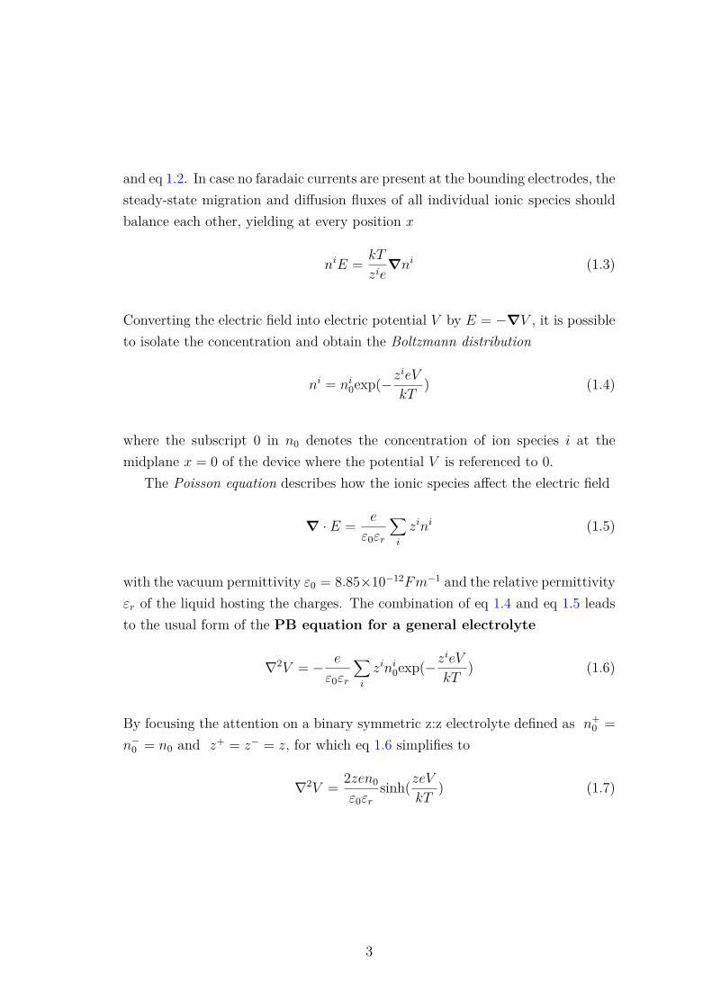
and eq 1.2. In case no faradaic currents are present at the bounding electrodes, thesteady-state migration and diffusion fluxes of all individual ionic species shouldbalance each other, yielding at every position x

niE = kT

zie∇ni (1.3)

Converting the electric field into electric potential V by E = −∇V , it is possibleto isolate the concentration and obtain the Boltzmann distribution

ni = ni0exp(−zieV

kT) (1.4)

where the subscript 0 in n0 denotes the concentration of ion species i at themidplane x = 0 of the device where the potential V is referenced to 0.

The Poisson equation describes how the ionic species affect the electric field

∇ · E = e

ε0εr

∑i

zini (1.5)

with the vacuum permittivity ε0 = 8.85×10−12Fm−1 and the relative permittivityεr of the liquid hosting the charges. The combination of eq 1.4 and eq 1.5 leadsto the usual form of the PB equation for a general electrolyte

∇2V = − e

ε0εr

∑i

zini0exp(−zieV

kT) (1.6)

By focusing the attention on a binary symmetric z:z electrolyte defined as n+0 =

n−0 = n0 and z+ = z− = z, for which eq 1.6 simplifies to

∇2V = 2zen0

ε0εrsinh(zeV

kT) (1.7)

3

Converting this equation into its dimensionless planar form gives

∂2V

∂x2 = λ0sinh(V ) (1.8)

with

V ≡ zeV

kT(1.9)

λ0 ≡2n0z

2e2d2

ε0εrkT(1.10)

where dimensionless position x = x/d, dimensionless voltage V and dimensionlessconcentration (at the midplane) λ0 are used.At this midplane x = 0, we define the zero reference of the potential V = 0, andbecause of the symmetry in eq 1.7 and 1.8, the potentials at both ends of thedevice will become opposite (equal to ± 1/2 ; see Figure 1.1).

1.1.1 Gouy-Chapman Solution

The Gouy-Chapman Solution (GC) is derived in numerous leading textbooks asa solution of the planar PB eq 1.7. However, the GC solution is not its generalsolution, since it makes a further assumption! In most of the textbooks, it isderived for the case of a single isolated charged plate immersed in electrolyte.Here the derivation is not reported but, analyzing the solution for the extendedcase of two oppositely charged plates, it will become evident how the physicalmeaning of the GC solution can fail.The further assumption of the GC approach is that there exists a region wherethe electric field is negligibly small. For the special case of two identically chargedplates, this assumption is fully justified since the midplane by symmetry has zerofield. However, in all other cases, this implies the presence of a "bulk electrolyte"region. From the Boltzmann eq 1.4, it follows that uniform potential (zero field)implies uniform concentration of all ionic species ("bulk"). Under electroneutrality

4

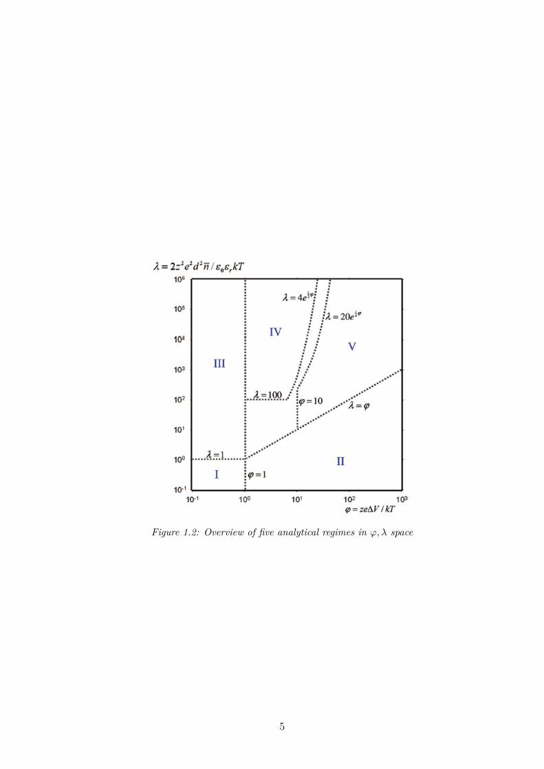
Figure 1.2: Overview of five analytical regimes in ϕ, λ space

5

conditions, this "bulk" region forms a trivial solution of the PB eq 1.6. For a singlecharged plate, it makes sense to assume "bulk electrolyte" at infinity. However,for the case of two oppositely charged plates, one cannot a priori justify the GCassumption ∂V /∂x|x=0 = 0. Nevertheless, if one make this assumption, then itfollows that

∂V

∂x= −

√4λ0

∣∣∣∣sinh(12 V

)∣∣∣∣ (1.11)

Solving this from the lower boundary x = −1/2 where V = 1/2 gives

V = 2ln1 + tanh

(18ϕ)exp

(−√λ0(

12 + x

))1− tanh

(18ϕ)exp

(−√λ0(

12 + x

)) −1

2 ≤ x < 0

V = 2ln1− tanh

(18ϕ)exp

(−√λ0(

12 − x

))1 + tanh

(18ϕ)exp

(−√λ0(

12 − x

)) 0 < x ≤ −1

2 (1.12)

Equation 1.12 is referred to as the GC solution, describing the potential profile asa function of the dimensionless midplane concentration λ0 and electrode poten-tial difference ϕ. This GC solution is widely used, often to successfully explainmeasurement results. It is useful, however, to investigate a posteriori the reason-ability of the "zero field" assumption, by calculating the first order estimates ofV and ∂V /∂x at the midplane x = 0 with eq 1.12:

V

∣∣∣∣∣∣x=0

' 4tanh(1

8ϕ)exp

(−1

4

√λ0)

(1.13)

∂V

∂x

∣∣∣∣∣∣x=0

'√

4λ02tanh(1

8ϕ)exp

(−1

4

√λ0)

(1.14)

In recalling both assumptions, the midplane potential estimate V |x=0 should bemuch lower than the maximum potential (1/2)ϕ and the midplane field estimate

6

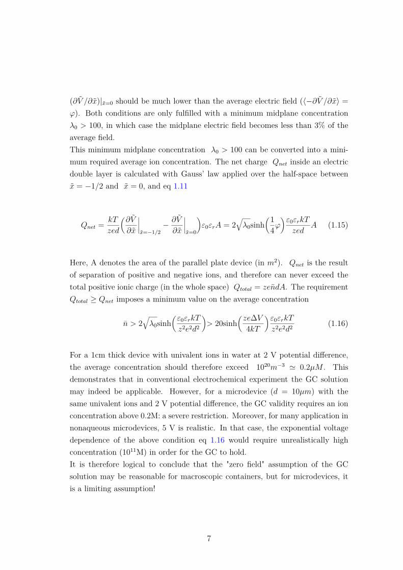
(∂V /∂x)|x=0 should be much lower than the average electric field (〈−∂V /∂x〉 =ϕ). Both conditions are only fulfilled with a minimum midplane concentrationλ0 > 100, in which case the midplane electric field becomes less than 3% of theaverage field.This minimum midplane concentration λ0 > 100 can be converted into a mini-mum required average ion concentration. The net charge Qnet inside an electricdouble layer is calculated with Gauss’ law applied over the half-space betweenx = −1/2 and x = 0, and eq 1.11

Qnet = kT

zed

(∂V

∂x

∣∣∣∣x=−1/2

− ∂V

∂x

∣∣∣∣x=0

)ε0εrA = 2

√λ0sinh

(14ϕ)ε0εrkT

zedA (1.15)

Here, A denotes the area of the parallel plate device (in m2). Qnet is the resultof separation of positive and negative ions, and therefore can never exceed thetotal positive ionic charge (in the whole space) Qtotal = zendA. The requirementQtotal ≥ Qnet imposes a minimum value on the average concentration

n > 2√λ0sinh

(ε0εrkT

z2e2d2

)> 20sinh

(ze∆V4kT

)ε0εrkT

z2e2d2 (1.16)

For a 1cm thick device with univalent ions in water at 2 V potential difference,the average concentration should therefore exceed 1020m−3 ' 0.2µM . Thisdemonstrates that in conventional electrochemical experiment the GC solutionmay indeed be applicable. However, for a microdevice (d = 10µm) with thesame univalent ions and 2 V potential difference, the GC validity requires an ionconcentration above 0.2M: a severe restriction. Moreover, for many application innonaqueous microdevices, 5 V is realistic. In that case, the exponential voltagedependence of the above condition eq 1.16 would require unrealistically highconcentration (1011M) in order for the GC to hold.It is therefore logical to conclude that the "zero field" assumption of the GCsolution may be reasonable for macroscopic containers, but for microdevices, itis a limiting assumption!

7

1.1.2 Complete Solution

To obtain the complete solution one has to return to the Poisson-Boltzmann equa-tion and solve it without assuming the presence of a "bulk electrolyte" region withzero field. Again, consider a symmetrical z:z electrolyte: z+ = −z− = z. Chargeneutrality over the device as a whole dictates

∫ d/2−d/2 n

−dx =∫ d/2−d/2 n

+dx = nd.

A total potential difference ∆V is applied between both electrodes (separatedby a distance d), and therefore the integrated electric field should be equal to∫ d/2−d/2Edx = ∆V . These quantities can be used for defining the following dimen-sionless variables

x ≡ x

dn± ≡ n±d∫

n±dx= n±

nE ≡ Ed∫

Edx= Ed

∆V (1.17)

Dimensionless parameters related to the applied voltage and average concentra-tion are defined as follows

ϕ ≡ ze∆VkT

and λ ≡ 2nz2e2d2

ε0εrkT(1.18)

Then eq 1.3 and eq 1.5 can be written as

ϕn±E = ±∂n±

∂x(1.19)

ϕ∂E

∂x= 1

2λ(n+ − n−) (1.20)

The solution of eq 1.19 and eq 1.20 is fully equivalent to the Poisson-Boltzmannformulation of eq 1.8, except from the use of λ (average concentration) as aparameter instead of λ0 (midplane concentration). The solution applies bothto strong and to weak electrolytes, as long as the average number of ions (andtherefore the average concentration n) is known in the steady-state situation.

8

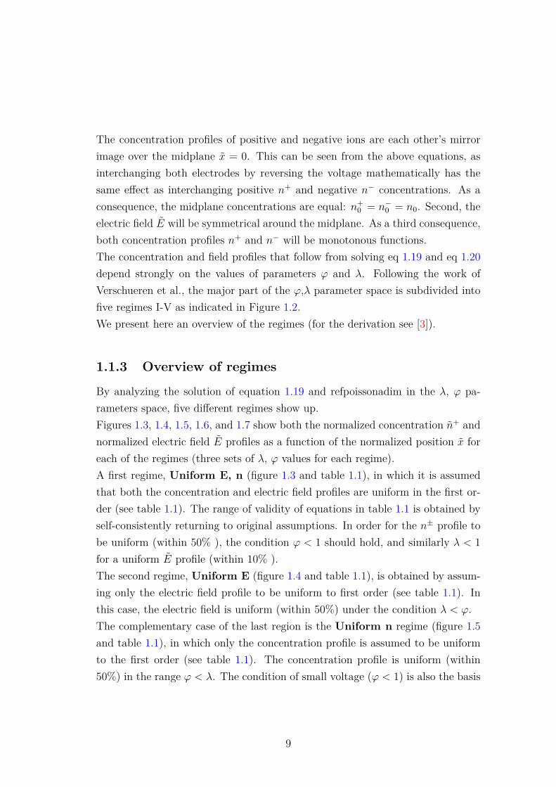
The concentration profiles of positive and negative ions are each other’s mirrorimage over the midplane x = 0. This can be seen from the above equations, asinterchanging both electrodes by reversing the voltage mathematically has thesame effect as interchanging positive n+ and negative n− concentrations. As aconsequence, the midplane concentrations are equal: n+

0 = n−0 = n0. Second, theelectric field E will be symmetrical around the midplane. As a third consequence,both concentration profiles n+ and n− will be monotonous functions.The concentration and field profiles that follow from solving eq 1.19 and eq 1.20depend strongly on the values of parameters ϕ and λ. Following the work ofVerschueren et al., the major part of the ϕ,λ parameter space is subdivided intofive regimes I-V as indicated in Figure 1.2.We present here an overview of the regimes (for the derivation see [3]).

1.1.3 Overview of regimes

By analyzing the solution of equation 1.19 and refpoissonadim in the λ, ϕ pa-rameters space, five different regimes show up.Figures 1.3, 1.4, 1.5, 1.6, and 1.7 show both the normalized concentration n+ andnormalized electric field E profiles as a function of the normalized position x foreach of the regimes (three sets of λ, ϕ values for each regime).A first regime, Uniform E, n (figure 1.3 and table 1.1), in which it is assumedthat both the concentration and electric field profiles are uniform in the first or-der (see table 1.1). The range of validity of equations in table 1.1 is obtained byself-consistently returning to original assumptions. In order for the n± profile tobe uniform (within 50% ), the condition ϕ < 1 should hold, and similarly λ < 1for a uniform E profile (within 10% ).The second regime, Uniform E (figure 1.4 and table 1.1), is obtained by assum-ing only the electric field profile to be uniform to first order (see table 1.1). Inthis case, the electric field is uniform (within 50%) under the condition λ < ϕ.The complementary case of the last region is the Uniform n regime (figure 1.5and table 1.1), in which only the concentration profile is assumed to be uniformto the first order (see table 1.1). The concentration profile is uniform (within50%) in the range ϕ < λ. The condition of small voltage (ϕ < 1) is also the basis

9

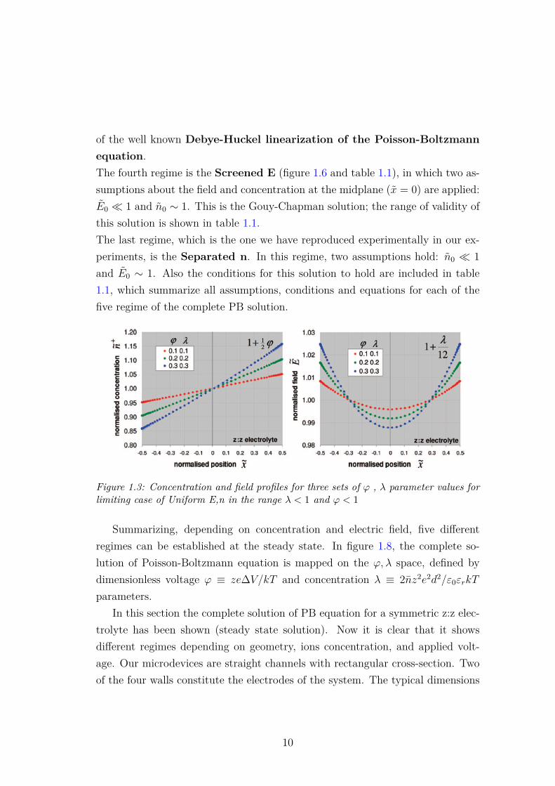
of the well known Debye-Huckel linearization of the Poisson-Boltzmannequation.The fourth regime is the Screened E (figure 1.6 and table 1.1), in which two as-sumptions about the field and concentration at the midplane (x = 0) are applied:E0 1 and n0 ∼ 1. This is the Gouy-Chapman solution; the range of validity ofthis solution is shown in table 1.1.The last regime, which is the one we have reproduced experimentally in our ex-periments, is the Separated n. In this regime, two assumptions hold: n0 1and E0 ∼ 1. Also the conditions for this solution to hold are included in table1.1, which summarize all assumptions, conditions and equations for each of thefive regime of the complete PB solution.

Figure 1.3: Concentration and field profiles for three sets of ϕ , λ parameter values forlimiting case of Uniform E,n in the range λ < 1 and ϕ < 1

Summarizing, depending on concentration and electric field, five differentregimes can be established at the steady state. In figure 1.8, the complete so-lution of Poisson-Boltzmann equation is mapped on the ϕ, λ space, defined bydimensionless voltage ϕ ≡ ze∆V/kT and concentration λ ≡ 2nz2e2d2/ε0εrkT

parameters.In this section the complete solution of PB equation for a symmetric z:z elec-

trolyte has been shown (steady state solution). Now it is clear that it showsdifferent regimes depending on geometry, ions concentration, and applied volt-age. Our microdevices are straight channels with rectangular cross-section. Twoof the four walls constitute the electrodes of the system. The typical dimensions

10

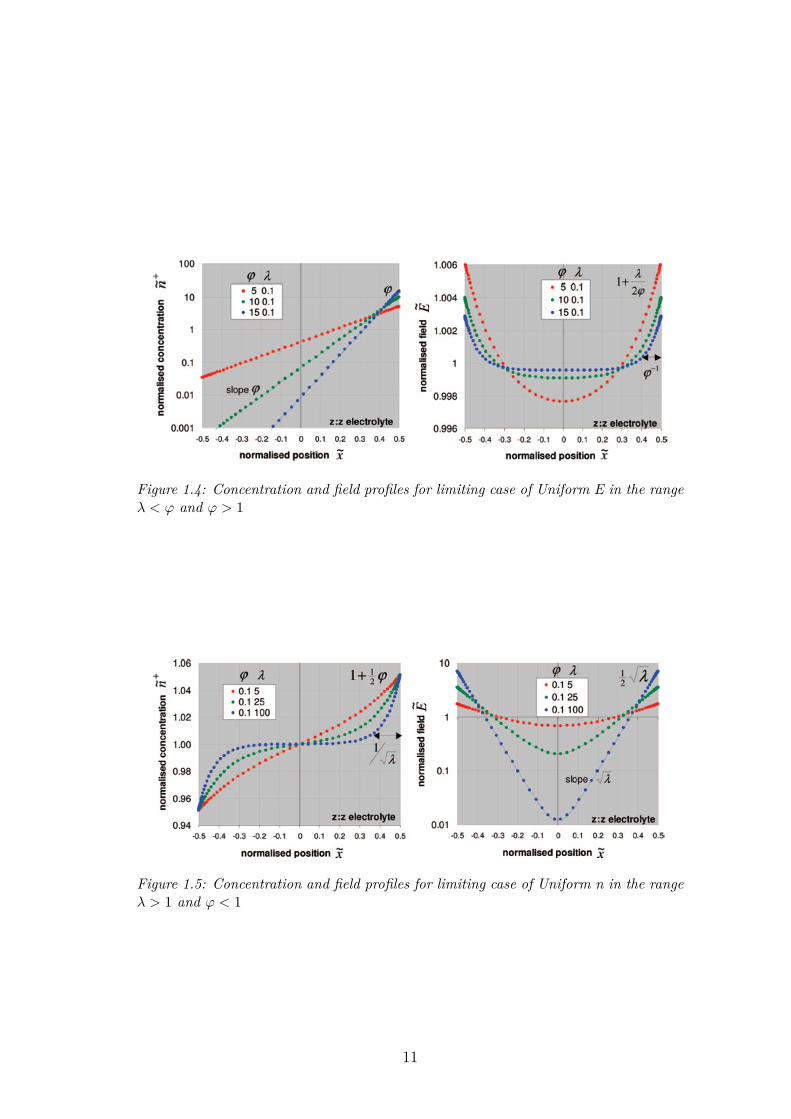
Figure 1.4: Concentration and field profiles for limiting case of Uniform E in the rangeλ < ϕ and ϕ > 1

Figure 1.5: Concentration and field profiles for limiting case of Uniform n in the rangeλ > 1 and ϕ < 1

11

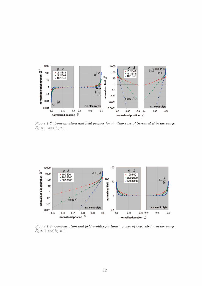
Figure 1.6: Concentration and field profiles for limiting case of Screened E in the rangeE0 1 and n0 ' 1

Figure 1.7: Concentration and field profiles for limiting case of Separated n in the rangeE0 ' 1 and n0 1

12

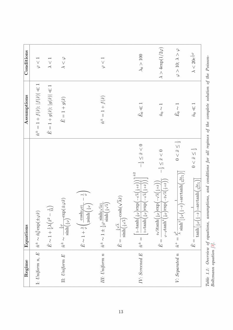
Regim

eEqu

ations

Assum

ptions

Con

dition

s

I:Uniform

n,E

n±∼n± 0exp(±ϕx

)n±

=1

+f

(x);|f

(x)|

1ϕ<

1

E∼

1+

1 2λ( x

2−

1 12

)E

=1

+g(x

);|g

(x)|

1λ<

1

II:U

niform

En±∼

1 2ϕ

sinh( 1 2

ϕ

) exp(±ϕx

)E

=1

+g(x

)λ<ϕ

E∼

1+

λ ϕ

cosh(ϕx

)

2sinh( 1 2

ϕ

) −1 ϕ

III:

Uniform

nn±∼

1±

1 2ϕsin

h(√λx

)

sinh( 1 2

√λ

)n±

=1

+f

(x)

ϕ<

1

E=

1 2√λ

sinh( 1 2

√λ

) cosh(√λx

)

IV:S

creenedE

n±

= 1−

tanh( 1 8

ϕ

) exp( −√

λ

( 1 2+x

))1+tanh( 1 8

ϕ

) exp( −√

λ

( 1 2+x

)) ±2

−1 2≤x<

0E

0

1λ

0>

100

E=

4√λtanh( 1 8

ϕ

) exp( −√

λ

( 1 2+x

))ϕ−ϕtanh

2( 1 8

ϕ

) exp( −2√

λ

( 1 2+x

))−

1 2≤x<

0n

0∼

1λ>

4exp

(1/2ϕ

)

V:S

eparated

nn

+=

ϕ2 λ

1

sinh2[ 1 2ϕ

( 1 2−x

) +arctan

h( 2ϕ2ϕ

+λ

)]0<x≤

1 2E

0∼

1ϕ>

10;λ

>ϕ

E=

1

tanh[ 1 2ϕ

( 1 2−x

) +arctan

h( 2ϕ2ϕ

+λ

)]0<x≤

1 2n

0

1λ<

20e

1 4ϕ

Table1.1:

Overview

ofequa

tions,assumptions,an

dcond

ition

sforallregimes

ofthecompletesolutio

nof

thePo

isson-

Boltzman

nequa

tion[3].

13

Figure 1.8: Overview of the regimes defined by the ratio of the midplane concentrationand field.

are shown in table 1.1.3. Following the theoretical framework of the previoussection we can estimate that, if a voltage of 2V is applied between two elec-trodes having a gap of 50µm, and the solution that flows into the channel has aconcentration of 300 ppm of KCl, then

ϕ = 77.81, and λ = 1.1× 108

From figure 1.2 it can be noticed that there are three conditions to be in theseparated n regime:

• λ = 1.1× 108 > ϕ = 77.8

• ϕ = 77.8 > 10

14

• λ = 1.1× 108 < 20e 14ϕ = 5.62× 109

All conditions are fulfilled, so the regime of the PB solution is the "Separatedn". These combination of applied voltage, ions concentration, and geometry, havebeen reproduced experiemtally (adding the flowrate). The results are shown infigure 4.17 (see the starting conditions). With the same conditions, but for lowerconcentrations, the PB regime is still the separated n (being ϕ = 77.8 and λ equalto 4.5 × 104, 1.1 × 106, and 1.1 × 107 respectively for DI water, 3ppm, and 30ppm of KCl).

Lenght Width Electrodes Gap[m] [m] [m]

3× 10−2; 9× 10−2 10−4; 10−3 5× 10−6; 3× 10−4

The idea is to use this separated regime to purify the flowing fluid from allion species included in traditional tapwater (Ca2+; K+; Cl−; Na+; ...). Indeed,inside the device, water streams through a narrow channel, where in two stages:mineral ions are separated by electric fields towards the sides of the channels,then the stream is split into a purified main stream and a concentrated wastestream.Let’s consider a 300 ppm solution of KCl diluted in DI water. If this solution flowswithin the microchannel while a voltage of 5V is applied between the electrodes,then, at the outlet of the channel, the central part of the device will be almostpurified from the ions, while the side regions near the electrodes will containalmost the entire amount of charged species.

15

1.2 Complete physical framework

1.2.1 Convection

Three transport mechanisms are present in our picture. Two of them are Migra-tion and Diffusion of charged species, which both occur from one wall of thechannel to the opposite charged wall; these two mechanisms have been describedin the previous section.The third mechanism is the convection of fluid. The latter occurs in the samedirection of the length of the channel, then being transversal to the migration ofions.Each of these mechanisms has a different driving force. Migration of ions is gen-erated by a potential gradient (electric field), diffusion of charged species occursdue to a concentration gradient, and convection flow is driven by a pressure dif-ference within the length of the channel.Analytical expressions for transversal transport mechanisms have already beenderived (PB equation). Due to the small dimensions of the devices with whichwe are dealing, the flow regime is basically laminar and Reynolds number (Re)is low

Re = ρuL

µ(1.21)

where ρ [Kg·m−3] and µ [Pa·s] are, respectively, the density and the dynamicviscosity of the fluid, L is the characteristic length, and u the mean velocity ofthe object relative to the fluid).To give a pratical comparison, we can calculate which is the value of Re forexperimental conditions of figure 4.17. In this case (for all solutions studied theviscosity is the same), L = 50 × 10−6 m, µH2O = 8.9 × 10−4 Pa·s, ρH2O = 103

Kg/m3, and v=13.3 mm/s, thus Re = 7.5× 10−1.For a straight channel, with a general cross-section, the expression for the flowcan be derived by solving the Navier-Stokes problem. The solution is a pressure-driven, steady-state flow, also known as Poiseuille flow or Hagen-Poiseuille flow.

16

This class is of major importance for the basic understanding of liquid handlingin lab-on-a-chip and microchannel systems. In a Poiseuille flow the fluid is driventhrough a long, straight, and rigid channel by imposing a pressure differencebetween the two ends of the channel.The length of the channel is parallel to the x axis, and it is assumed to betranslation invariant in that direction. The constant cross-section in the yz planeis denoted C with boundary ∂C, respectively. A constant pressure difference ∆Pis maintained over a segment of length L of the channel, i.e., P (0) = p0 + ∆Pand p(L) = p0. The gravitational force is balanced by a hydrostatic pressuregradient in the vertical direction. These two forces are therefore left out of thetreatment. The translation invariance of the channel in the x direction combinedwith the vanishing of forces in the yz plane implies the existence of a velocity fieldindependent of x, while only its x component can be non-zero, v(r) = vx(y, z) ·ex.Consequently (v · ∇)v = 0 and the steady-state Navier–Stokes equation becomes

v(r) = vx(y, z) · ex (1.22)

0 = η∇2[vx(y, z) · ex]−∇p (1.23)

Since y and z components of the velocity field are zero, it follows that ∂yp = 0 and∂zp = 0, and consequently that the pressure field only depends on x, p(r) = p(x).Using this result the x component of the Navier–Stokes equation becomes

η(∂2y + ∂2

z )vx(y, z) = ∂xp(x) (1.24)

Here it is seen that the left-hand side is a function of y and z while the right-handside is a function of x. The only possible solution is thus that the two sides of theNavier–Stokes equation equal the same constant. However, a constant pressuregradient ∂xp(x) implies that the pressure must be a linear function of x, and using

17

the boundary conditions for the pressure we obtain

p(r) = ∆pηL

(L− x) + p0 (1.25)

Figure 1.9: The Poiseuille flow problem in a channel, which is translation invariantin the x direction, and which has an arbitrarily shaped cross-section C in the yz plane.The boundary of C is denoted ∂C. The pressure at the left end, x = 0, is an amount∆p higher than at the right end, x = L [18].

With this we finally arrive at the second-order partial differential equation thatvx(y, z) must fulfil in the domain C given the usual no-slip boundary conditionsat the solid walls of the channel described by ∂C,

(∂2y + ∂2

z )vx(y, z) = −∆pηL

(y, z) ∈ C (1.26)

vx(y, z) = 0 (y, z) ∈ ∂C (1.27)

Once the velocity field is determined it is possible to calculate the so-called flowrate Q, which is defined as the fluid volume transported by the channel per unittime. For compressible fluids it becomes important to distinguish between theflow rate Q and the mass flow rate Qmass defined as the discharged mass per unittime. In the case of the geometry of Figure 1.9 we have

Q ≡∫Cdydzvx(y, z) (1.28)

18

Qmass ≡∫Cdydzρvx(y, z) (1.29)

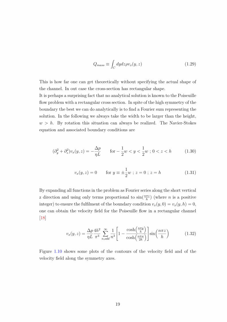
This is how far one can get theoretically without specifying the actual shape ofthe channel. In out case the cross-section has rectangular shape.It is perhaps a surprising fact that no analytical solution is known to the Poiseuilleflow problem with a rectangular cross section. In spite of the high symmetry of theboundary the best we can do analytically is to find a Fourier sum representing thesolution. In the following we always take the width to be larger than the height,w > h. By rotation this situation can always be realized. The Navier-Stokesequation and associated boundary conditions are

(∂2y + ∂2

z )vx(y, z) = −∆pηL

for− 12w < y <

12w ; 0 < z < h (1.30)

vx(y, z) = 0 for y ≡ ±12w ; z = 0 ; z = h (1.31)

By expanding all functions in the problem as Fourier series along the short verticalz direction and using only terms proportional to sin(nπz

h) (where n is a positive

integer) to ensure the fulfilment of the boundary condition vx(y, 0) = vx(y, h) = 0,one can obtain the velocity field for the Poiseuille flow in a rectangular channel[18]

vx(y, z) = ∆pηL

4h2

π3

∞∑n,odd

1n3

1−cosh

(nπyh

)cosh

(nπw2h

)sin(nπz

h

)(1.32)

Figure 1.10 shows some plots of the contours of the velocity field and of thevelocity field along the symmetry axes.

19

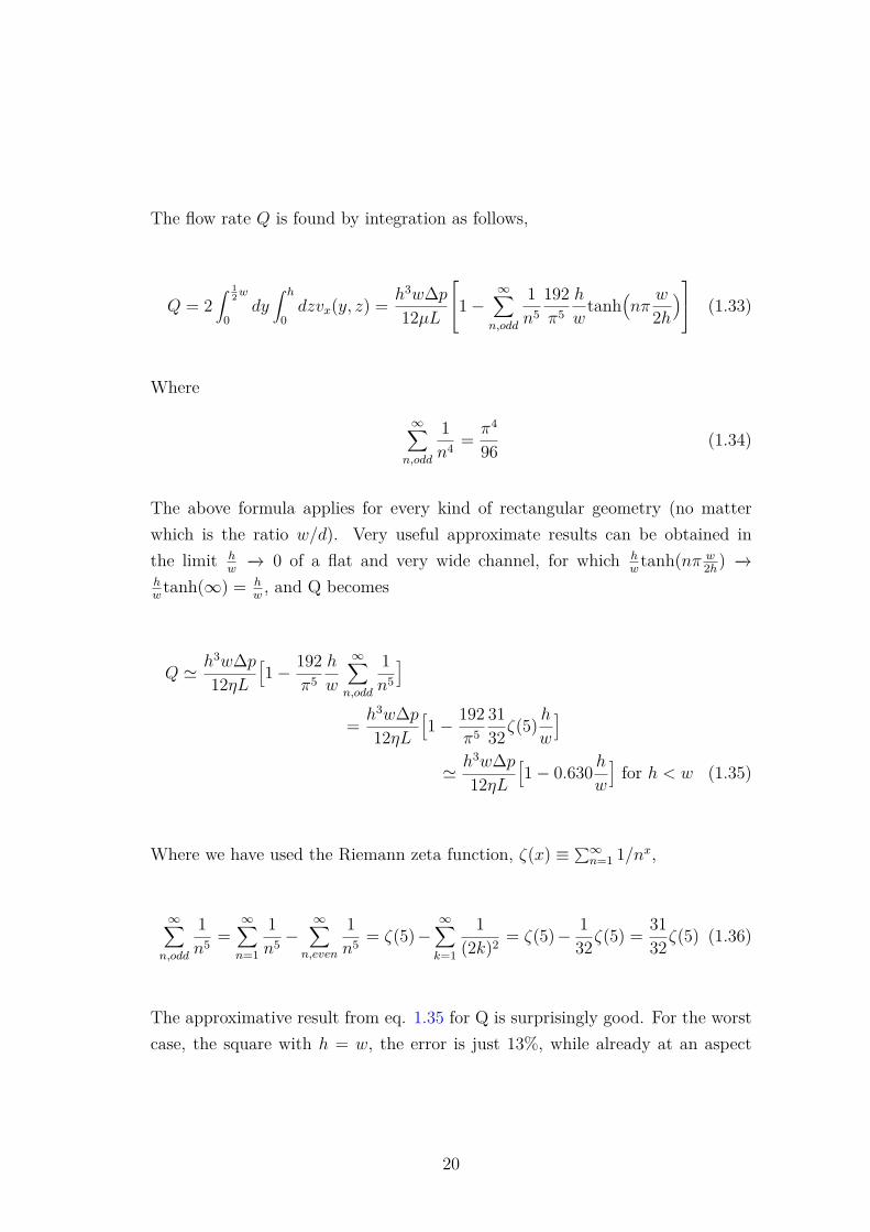
The flow rate Q is found by integration as follows,

Q = 2∫ 1

2w

0dy∫ h

0dzvx(y, z) = h3w∆p

12µL

1−∞∑

n,odd

1n5

192π5

h

wtanh

(nπ

w

2h) (1.33)

Where

∞∑n,odd

1n4 = π4

96 (1.34)

The above formula applies for every kind of rectangular geometry (no matterwhich is the ratio w/d). Very useful approximate results can be obtained inthe limit h

w−→ 0 of a flat and very wide channel, for which h

wtanh(nπ w

2h) −→hwtanh(∞) = h

w, and Q becomes

Q ' h3w∆p12ηL

[1− 192

π5h

w

∞∑n,odd

1n5

]

= h3w∆p12ηL

[1− 192

π53132ζ(5) h

w

]' h3w∆p

12ηL[1− 0.630 h

w

]for h < w (1.35)

Where we have used the Riemann zeta function, ζ(x) ≡ ∑∞n=1 1/nx,

∞∑n,odd

1n5 =

∞∑n=1

1n5 −

∞∑n,even

1n5 = ζ(5)−

∞∑k=1

1(2k)2 = ζ(5)− 1

32ζ(5) = 3132ζ(5) (1.36)

The approximative result from eq. 1.35 for Q is surprisingly good. For the worstcase, the square with h = w, the error is just 13%, while already at an aspect

20

ratio of a half, h = w/2, the error is down to 0.2% .

Figure 1.10: Contour lines for the velocity field vx(y, z) for the Poiseuille flow problemin a rectangular channel. The contour lines are shown in steps of 10 % of the maximalvalue vx(0, h2 ). (b) A plot of vx(y, h2 ) along the long center-line parallel to ey. (c) Aplot of vx(0, z) along the short center-line parallel to ez.

Until now we have considered the following processes:

• Fluid convection from the inlet to the outlet of the channel;

• Migration and Diffusion of ions from the bulk to the sides and from one sideto the other.In a real case, together with the above mentioned Migration and Diffusion ofcharged particles, there are a number of other physical-chemical phenomena thatoccur. The most important, which cannot be neglected, are

• Auto-ionization of water;

• Electrolysis at the electrodes surface.

The first is a bulk process [8], while the second one is a surface process (whichstrongly depends on applied voltage). Let’s describe how they work and how theyinfluence the performances of ions separation.

21

1.2.2 Autoionization of water

The self-ionization of water (also autoionization of water, and autodissociation ofwater) is an ionization reaction in pure water or an aqueous solution, in which awater molecule, H2O, loses the nucleus of one of its hydrogen atoms to become ahydroxide ion, OH−. The hydrogen nucleus, H+, immediately protonates anotherwater molecule to form hydronium, H3O

+. It is an example of autoprotolysis,and exemplifies the amphoteric nature of water.Chemically pure water has a conductivity of

σ = 0.055µS/cm (1.37)

The conductivity of pure water and any aqueous solution, according to Svante-Arrhenius theories, must be due to the presence of ions. The ions are producedby the self-ionization reaction:

H2O H+ +OH− (1.38)

This equilibrium applies to pure water and any aqueous solution. The chemicalequilibrium constant, Keq, for this reaction, is given by

Keq = [H+][OH−][H2O] (1.39)

If the concentration of the dissolved solutes is not very high, the concentrationof [H2O] can be taken as being constant at ca 55.5 M.The Ionization constant (Dissociation constant, Self-Ionization constant, orIonic product) of water, symbolized with Kw, is given by

Kw = [H+][OH−] = Keq × [H2O] (1.40)

22

Where [H+] is the concentration ofH+, and [OH−] is the concentration of hydrox-ide ion. At 25’C Kw is approximately equal to 1 × 10−14 M2. Water moleculesdissociate into equal amounts of [H+] and [OH−], so their concentrations areequal to ca 1× 10−7 mol dm−3.It is useful to study the kinetics of equilibrium 1.38. The following relation forthe time derivative of [H+] and [OH−] holds

∂[H+]∂t

= ∂[OH−]∂t

= kD · [H2O]−Krec · [H+][OH−] (1.41)

Thus, the equilibrium constant can be written in terms of kD and krec as follows

Keq = kDkrec

= kw[H2O] (1.42)

The recombination process [10] is not instantaneous, but is governed by a finiterate. According to [10], the water recombination rate is given by

krec = 1.4× 1011[M−1 · s−1] (1.43)

Or, in [m3/s]

1.4× 1011

6× 1026 = 2.33× 10−16[m3/s] (1.44)

With equation 1.42 and 1.43, knowing that Kw = 10−14 M2, it is possible toobtain a relation for kD and quantify it

kD = krec · kw[H2O] = 1.12× 1011[M−1s−1] · 10−14[M2]

55.5[M] = 113.76 hours (1.45)

23

From this result, it is clear that the dissociation of water is a very slow process.What makes it effective is the high concentration of water molecules, which com-pensates the rate of the reaction.A solution in which H+ and OH− concentrations equal each other is consideredas a neutral solution.Pure H2O is a neutral solution, but most H2O samples contain impurities. If animpurity is an acid or base this will affect the concentration of hydronium andhydroxide ions. Water samples which are exposed to air will absorb the acid car-bon dioxide and concentration of H+ will increase. The concentration of OH−

will decrease in such a way that the product [H+][OH−] remains constant forfixed temperature and pressure.

1.2.3 Electrolysis

Depending on applied voltage, reactions at electrodes can occur [15]; [16]. As willbecome clear later (Potential step Voltammetry section), when a series of differentvoltage step amplitudes is applied, one can obtain an I-V curve, in which thesteady state current at each amplitude is plotted as a function of applied voltage[9]. In this plot, depending on electrode materials, three different regions can beidentified: moving from lower to higher voltages, a first region in which currentincreases with voltage; a second region in which the current shows a plateau(same current for different voltages); and a third part, which is characterized bya strong exponential increase in current.

1.2.3.1 Theory of electrolysis

Typical experiments on electrolysis involve high concentrations of acid added tothe solution. In this way, one achieves standard conditions (e.g. concentrationsof solutions is 1 M, temperature is 25C, and all gasses are at 1 bar), underwhich one can use directly the standard potential of an electrode to estimate thecurrent.

24

However, in our case, we are not in standard conditions. Three reactions occurin our experiments, involving generation of H+ and OH−, together with H2 andO2. These are a cathode reaction

H+ + e− −→ 12H2 (1.46)

or

H2O + e− −→ OH− + 12H2(g) (1.47)

And an anode reaction

12H2O −→ H+ + 1

4O2(g) + e− (1.48)

Each of these has an electrode potential, which establishes the voltage requiredto drive the reaction. The electrode potential can be calculated using the Nernstequation applied at each reaction. By enumerating equation 1.46 with subscript 1,equation 1.47 with subscript 2, and equation 1.48 with subscript 3, the potentialsare

V1 = V0,1 −RT

Fln[a1/2

H2

aH+

](1.49)

V2 = V0,2 −RT

Fln[a

1/2H2 aOH−

](1.50)

V3 = V0,3 −RT

Fln[ 1a

1/4O2 aH+

](1.51)

where symbol a indicates the activity of each species, F is the Faraday constant(i.e. 96,485 [C/mol]), and the subscript 0 indicates the standard electrode poten-tial (i.e. V0,1 = 0 V; V0,2 = −0.8277 V; V0,3 = 1.23 V). Depending on the phase

25

of each species, the activity can be related to other quantities. For diluted ionsthe following relation holds

ai = cic0

(1.52)

where c0 is the standard concentration.For ideal gases, the activity can be related to partial pressure with followingequation

ai = pip0

(1.53)

where p0 is the standard pressure. Also dissolved gases are present in our case.Their activity can be related to concentrations using Henry’s law

p = kHceq (1.54)

Then,

ai = pip0

= kHcip0

= kHcikHc0

= cic0

(1.55)

where the subscript 0 here indicates concentration at standard p, T. It can eas-ily be demonstrated that activity of dissolved gases can be related also to thesaturation concentration. Consider a generic gas-solution equilibrium

A(g) ←−−→ A(aq) (1.56)

for each species the chemical potential is expressed by

µg = µ0 +RT ln(ag)

26

µaq = µ0 +RT ln(aaq) (1.57)

thus, at equilibrium, µg = µaq gives ag = aaq, being µ0,g = µ0,aq [17].For ideal gases, relation 1.53 holds. Nevertheless, Henry’s law (1.54) states thatc ∝ p, so

aaq = ag = pip0

= kHceqkHceq,p=p0

= ceqcsat

(1.58)

where csat ≡ p0kH

(concentration at p = p0). When p = p0, c ≡ csat, thus the ac-tivity of dissolved gases is directly related to the ratio of concentration of speciesi and its saturation concentration csat.In our reactions, the only gases species are O2 and H2. Their saturation concen-trations (when p = p0) are 1.38 mM for O2 and 0.807 mM for H2.Substituting relations 1.52, 1.53, and 1.55 into equations 1.49, 1.50, and 1.51gives

V1 = V0,1 − 0.059[V] log[a1/2

H2

aH+

]= 0[V] − 0.059[V]

[pHcath + 1

2 log[aH2 ]]

(1.59)

V2 = V0,2 − 0.059[V] log[a

1/2H2 aOH−

]=

= −0.8277[V] − 0.059[V][− pOHcath + 1

2 log[aH2 ]]

=

= −0.8277[V] − 0.059[V] · 14− 0.059[V][pHcath + 1

2 log[aH2 ]]

(1.60)

Thus

V1 = V2 = −0.059[V][pHcath + 1

2[aH2 ]]

(1.61)

27

Then, for anode reaction

V3 = V0,3 − 0.059[V] log[ 1a

1/4O2 aH+

]= 1.23[V] − 0.059[V]

[pHan −

14 log[aO2 ]

](1.62)

So, taking the difference between anode and cathode one obtain the relationbetween ∆V and ∆pH

∆V = V3 − V2 = 1.23[V] + 0.059[V][(pHcath − pHan) + 1

4 logaO2 + 12 logaH2

]=

= 1.23[V] + 0.059[V][∆pHc−a + 1

4 logaO2 + 12 logaH2

](1.63)

Equation 1.63 describes the relation between applied voltage and pH differencebetween cathode and anode.To know how the pH depends on applied potential, two approaches can be used:the first one uses the relation 1.4 to derive the pH dependence on applied poten-tial, while the second approach takes the definition of total chemical potential andapplies the equilibrium conditions to it. Now, we demonstrate that, by applyingseparately both different approaches, the same conclusion comes out.

Derivation from Gouy-Chapman

Equation 1.4 gives the distribution of concentration as a function of the dis-tance from a charged surface. Applying it to anode gives

nH+ = nH+ · e12−e∆VkT (1.64)

Using the definition of pH

28

pH = −log10nH+ = −log10

(nH+ · e

12−e∆VkT

)=

= −log10nH+ − log10e12−e∆VkT =

= −log10nH+ − 0.4312e∆VkT

(1.65)

By applying the same relation to cathode, and then taking the difference, thefollowing result comes out

∆pHcath−an = −0.43e∆EkT

= − ∆V0.059[V] (1.66)

Derivation from µtot at equilibrium

At constant pressure and temperature, Gibbs energy is minimal at equilib-rium: chemical potential is constant for each species:

µi =(∂G

∂Ni

)T,P,Nj 6=i

(1.67)

The total chemical potential µtot include an internal chemical potential µintand an external term, µext, which takes into account external sources of energy(e.g applied potential). The expression for µtot is then

µtot = µint + µext = µ0 + µE + µchem = µ0 + zFV (x) +RT ln[n(x)

](1.68)

So, when µtot is constant

const = zFV (x) +RT ln[n(x)

](1.69)

29

which, rearranged, becomes

n(x) = const · e−zFRT

V (x) (1.70)

Using the Gouy-Chapman assumption (E|bulk = 0), the constant is equal to thebulk concentration n, thus giving a complete expression for n(x)

n(x) = n · e−zFRT

V (x) (1.71)

This expression can be manipulated by applying −log to all terms; the result is

−log[n(x)

]= −log(n) ·+ zF

RT ln(10)V (x) (1.72)

By applying this equation to both anode and cathode, and taking the difference,one obtain

pHcath − pHan = zF

RT ln(10)(Vcath − Van) = − ∆V0.059[V] (1.73)

Which coincides with equation 1.66. Furthermore, when chemical equilibrium isreached, the following conditions on chemical potential hold

∑µreact =

∑µprod

∑i

νiµi = 0 (1.74)

this conditions, combined with equation 1.68 results in Nernst equation

V = −∑i νiµ0,i

F∑i νizi

− RT

F∑i νizi

∑i

νiln(ni) = V0 −RT

nFlnQ (1.75)

30

1.2.3.2 Threshold voltage for electrolysis

We derived the equations describing the electrolysis mechanism, and showed howthe electrolysis reactions affect the pH of the system. Summarizing, we can statethat electrolysis is a non-equilibrium process which acts to reestablish a new equi-librium. To understand when electrolysis starts, it is necessary to individuate thethreshold voltage at which the equilibrium cannot be reached.From equation 1.63 and 1.73, since the saturation concentration value is 1.38mMfor O2 and 0.807mM for H2, it is clear that there is a limit on applied voltage,after which all dissolved gas species have already reached their saturation con-centration, and thus the ratio c/csat = 1. This threshold voltage can easily becalculated by setting to zero the value of activities terms in equation 1.63

∆Vthreshold = 1.23[V] + 0.059[V] ∆pHcath−an (1.76)

then, using equation 1.73, it comes out that

∆Vthreshold = 1.23[V] −∆V (1.77)

So, ∆V > ∆Vthreshold when ∆V >1.23[V]

2 = 0.61V . This is the voltage at whichelectrolysis starts, creating H+ and O2 at anode and OH− and H2 at cathode.The fact that the threshold is lower than 1.23V can also be interpreted as aneffect of migration. When a voltage is applied, H+ migrate towards cathode, andOH− towards anode; when they will reach the electrode, they will react to formH2 and O2 respectively, thus "pushing" both oxidation and reduction reactions toproduce more dissolved gases.

Now, we present a study on how electrolysis acts and modify the steady-stateshape of an i, V curve. Four different regimes will show up.

31

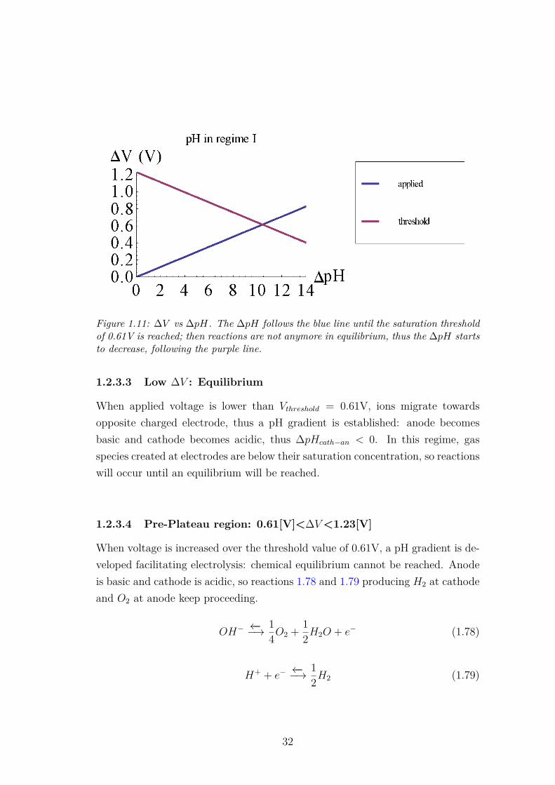
Figure 1.11: ∆V vs ∆pH. The ∆pH follows the blue line until the saturation thresholdof 0.61V is reached; then reactions are not anymore in equilibrium, thus the ∆pH startsto decrease, following the purple line.

1.2.3.3 Low ∆V : Equilibrium

When applied voltage is lower than Vthreshold = 0.61V, ions migrate towardsopposite charged electrode, thus a pH gradient is established: anode becomesbasic and cathode becomes acidic, thus ∆pHcath−an < 0. In this regime, gasspecies created at electrodes are below their saturation concentration, so reactionswill occur until an equilibrium will be reached.

1.2.3.4 Pre-Plateau region: 0.61[V]<∆V<1.23[V]

When voltage is increased over the threshold value of 0.61V, a pH gradient is de-veloped facilitating electrolysis: chemical equilibrium cannot be reached. Anodeis basic and cathode is acidic, so reactions 1.78 and 1.79 producing H2 at cathodeand O2 at anode keep proceeding.

OH−←−−→ 1

4O2 + 12H2O + e− (1.78)

H+ + e−←−−→ 1

2H2 (1.79)

32

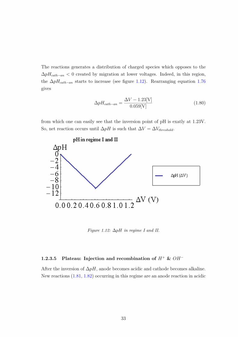
The reactions generates a distribution of charged species which opposes to the∆pHcath−an < 0 created by migration at lower voltages. Indeed, in this region,the ∆pHcath−an starts to increase (see figure 1.12). Rearranging equation 1.76gives

∆pHcath−an = ∆V − 1.23[V]0.059[V] (1.80)

from which one can easily see that the inversion point of pH is exatly at 1.23V.So, net reaction occurs until ∆pH is such that ∆V = ∆Vthreshold.

Figure 1.12: ∆pH in regime I and II.

1.2.3.5 Plateau: Injection and recombination of H+ & OH−

After the inversion of ∆pH, anode becomes acidic and cathode becomes alkaline.New reactions (1.81, 1.82) occurring in this regime are an anode reaction in acidic

33

environment

12H2O −→ H+ + 1

4O2(g) + e− (1.81)

and a cathode reaction in alkaline environment

H2O + e− −→ OH− + 12H2(g) (1.82)

The i, V curve has a plateau. As current is a monotonous increasing functionof overpotential η = ∆V −∆Vthreshold, this means that in the plateau region theoverpotential is constant

η = ∆V −∆Vthreshold = const = η0 (1.83)

thus, using expression 1.76, we can write

∆V − 1.23[V] − 0.059[V] ∆pHcath−an = η0 (1.84)

and so

∆pHcath−an = ∆V − 1.23[V] − η0

0.059[V] (1.85)

It is clear that ∆pHcath−an cannot increase above a certain threshold. Assuminga threshold of ∆pHcath−an = 12, if we include this into expression 1.76 we obtaina value for ∆V of 1.94V. Substituting this value into expression 1.85 gives a nulloverpotential. This can explain why in the plateau region we don’t see an increaseof current when applied voltage is varied in a appropriate range.

34

1.2.3.6 Very high ∆V : electrolysis and bubbles

Once the maximum pH gradient is reached, there is no other mechanism whichcan compensate the voltage. Every potential amplitude above the pH gradientthreshold is an overpotential, which generates charged species and bubbles at theelectrodes.

1.2.3.7 Expression for injection current

In the plateau region, electrolysis reactions occur at electrodes, which lead to theformation of H+ and OH−. This process is known as Injection of H+ and OH−

at electrodes.Consider a cross section (see figure 1.13) of the microchannel; left and right wallsconstitute the electrodes of the device. When a voltage is suddenly applied, H+

and OH− migrate towards opposite charged electrodes, and recombine in thebulk, thus contributing to measured current. At the electrodes, reactions occur,which lead to the generation of H+ and OH−.

Figure 1.13: Cross section of a sample

35

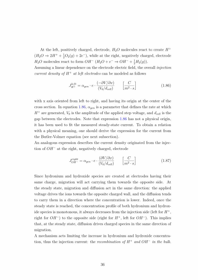
At the left, positively charged, electrode, H2O molecules react to create H+

(H2O −→ 2H+ + 12O2(g) + 2e−), while at the right, negatively charged, electrode

H2O molecules react to form OH− (H2O + e− −→ OH− + 12H2(g)).

Assuming a linear dependence on the electrode electric field, the overall injectioncurrent density of H+ at left electrodes can be modeled as follows

J leftH+ = αgen · e ·(−∂V/∂x)(V0/dcell)

[C

m2 · s

](1.86)

with x axis oriented from left to right, and having its origin at the center of thecross section. In equation 1.86, αgen is a parameter that defines the rate at whichH+ are generated, V0 is the amplitude of the applied step voltage, and dcell is thegap between the electrodes. Note that expression 1.86 has not a physical origin,it has been used to fit the measured steady-state current. To obtain a relationwith a physical meaning, one should derive the expression for the current fromthe Butler-Volmer equation (see next subsection).An analogous expression describes the current density originated from the injec-tion of OH− at the right, negatively charged, electrode

JrightOH− = αgen · e ·(∂V/∂x)(V0/dcell)

[C

m2 · s

](1.87)

Since hydronium and hydroxide species are created at electrodes having theirsame charge, migration will act carrying them towards the opposite side. Atthe steady state, migration and diffusion act in the same direction: the appliedvoltage drives the ions towards the opposite charged wall, and the diffusion tendsto carry them in a direction where the concentration is lower. Indeed, once thesteady state is reached, the concentration profile of both hydronium and hydrox-ide species is monotonous, it always decreases from the injection side (left for H+,right for OH−) to the opposite side (right for H+, left for OH−). This impliesthat, at the steady state, diffusion drives charged species in the same direction ofmigration.A mechanism acts limiting the increase in hydronium and hydroxide concentra-tion, thus the injection current: the recombination of H+ and OH− in the bulk.

36

Indeed, at the center of the channel (bulk region), H+ and OH− react to re-combine and form a water molecule. At the steady state, the rate at which H+

and OH− (1024m−3·s−) recombine balances the rate at which they are createdthrough injection.The main consequence of this mechanism is that if, at the steady state, the cur-rent at which injection and recombination balance each other is dominant overthe other processes, then the measured current (versus time) has to show a flathorizontal shape: this result is in agreement with our experiments (cfr fig 4.12).

1.2.3.8 Electrolysis at higher voltages: air & bubbles formation

If the applied voltage is increased, same reactions occur. The result is the for-mation of H2(g) and O2 (g) at the electrodes. The main difference betweenthe previous regime and the present is the impossibility of reaching equilibrium,since both the concentration of dissolved gases and the pH gradient have alreadyreached their limit. Here, every increase on applied voltage gives an overpotential,which increases the rate of electrolysis reactions. As mentioned in the previoussubsection, the Butler-volmer equation allows to calculate the current density re-sulting from the electrolysis mechanism. It describes how the electrical currenton an electrode depends on electrode potential, considering that both a cathodicand an anodic reaction occur on the same electrode.

i = i0 ·[exp

(αaNeFη

RT

)− exp

(− αcNeFη

RT

)](1.88)

where i is the electrode current densisty, i0 is the exchange current density, Tthe absolute temperature, Ne the number of electrons involved in the reaction, Fthe Faraday constant, αa and αc are the so-called anodic and cathodic transferdimensionless coefficient, and η is the overpotential.The above equation 1.88 refers to a system which is not limited by any masstransfer process from the bulk to the electrode surface. In the mass-transfer-

37

influenced conditions, a more general expression holds

i = i0 ·[n0(0, t)n∗0

exp(αaNeFη

RT

)− nr(0, t)

n∗rexp

(− αcNeFη

RT

)](1.89)

in which n0 and nr refer to the concentration of the oxidized and the reducedform, respectively. n(0, t) is the time-dependent concentration at the distancezero from the surface, while n∗0 and n∗r are bulk concentrations of the oxidizedand the reduced form, respectively. It can be easily noticed that expression 1.89simplifies to expression 1.88 when the concentration of the electroactive speciesat the surface equals to that in the bulk.The activation voltage, the speed and the products of described reactions aredetermined by the nature of the electrode material, even though the latter is notpart of the reaction’s stoichiometry. Because of this, such reactions are oftendescribed as examples of electrocatalysis. Much research is being conductedaimed at diminishing the voltage needed to affect water electrolysis. Voltages aslow as 1.6 V have been achieved by the use of catalytic electrodes.In our case, formation of hydrogen and oxygen at electrodes is an issue, sinceit causes air formation within the channel. For these reasons all choices havebeen made following the opposite goal: reduce the effect of electrolysis byfinding the material which shows the highest voltage to drive the airformation reaction.

1.3 Theoretical model based on RC network

As already stated, the physical model which represents the charge transportphenomena is well described by the Poisson-Nernst-Plank equations in a pla-nar geometry. In the previous section we described the physical picture andthe involved processes: migration and diffusion of ions, advection, electrolysis at

38

Figure 1.14: The electrolysis of water produces oxygen at the anode and hydrogen at thecathode. Ions from an electrolyte are necessary to provide conductivity but these playno role in the electrode reactions.

39

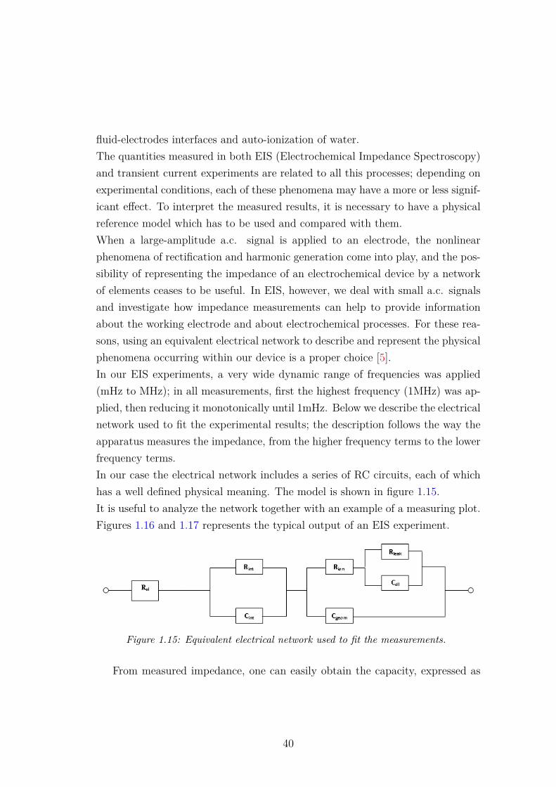
fluid-electrodes interfaces and auto-ionization of water.The quantities measured in both EIS (Electrochemical Impedance Spectroscopy)and transient current experiments are related to all this processes; depending onexperimental conditions, each of these phenomena may have a more or less signif-icant effect. To interpret the measured results, it is necessary to have a physicalreference model which has to be used and compared with them.When a large-amplitude a.c. signal is applied to an electrode, the nonlinearphenomena of rectification and harmonic generation come into play, and the pos-sibility of representing the impedance of an electrochemical device by a networkof elements ceases to be useful. In EIS, however, we deal with small a.c. signalsand investigate how impedance measurements can help to provide informationabout the working electrode and about electrochemical processes. For these rea-sons, using an equivalent electrical network to describe and represent the physicalphenomena occurring within our device is a proper choice [5].In our EIS experiments, a very wide dynamic range of frequencies was applied(mHz to MHz); in all measurements, first the highest frequency (1MHz) was ap-plied, then reducing it monotonically until 1mHz. Below we describe the electricalnetwork used to fit the experimental results; the description follows the way theapparatus measures the impedance, from the higher frequency terms to the lowerfrequency terms.In our case the electrical network includes a series of RC circuits, each of whichhas a well defined physical meaning. The model is shown in figure 1.15.It is useful to analyze the network together with an example of a measuring plot.Figures 1.16 and 1.17 represents the typical output of an EIS experiment.

Figure 1.15: Equivalent electrical network used to fit the measurements.

From measured impedance, one can easily obtain the capacity, expressed as

40

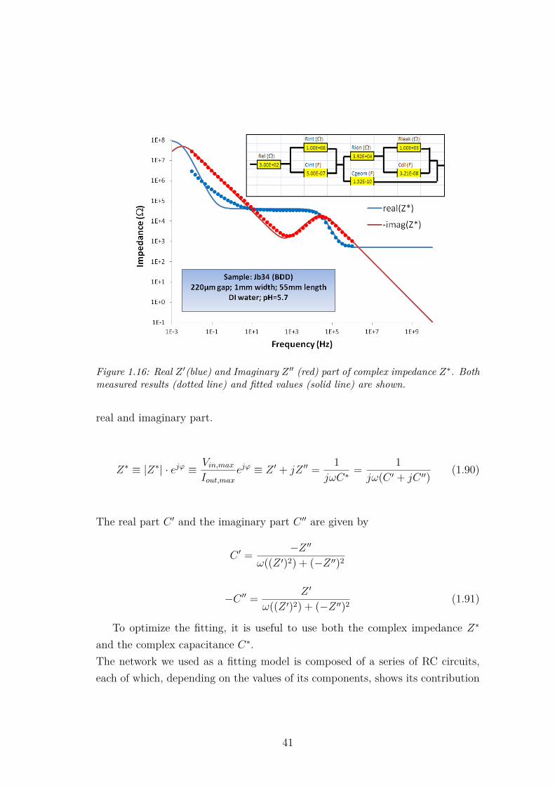
Figure 1.16: Real Z ′(blue) and Imaginary Z ′′ (red) part of complex impedance Z∗. Bothmeasured results (dotted line) and fitted values (solid line) are shown.

real and imaginary part.

Z∗ ≡ |Z∗| · ejϕ ≡ Vin,maxIout,max

ejϕ ≡ Z ′ + jZ ′′ = 1jωC∗

= 1jω(C ′ + jC ′′) (1.90)

The real part C ′ and the imaginary part C ′′ are given by

C ′ = −Z ′′

ω((Z ′)2) + (−Z ′′)2

−C ′′ = Z ′

ω((Z ′)2) + (−Z ′′)2 (1.91)

To optimize the fitting, it is useful to use both the complex impedance Z∗

and the complex capacitance C∗.The network we used as a fitting model is composed of a series of RC circuits,each of which, depending on the values of its components, shows its contribution

41

Figure 1.17: Real C ′ (blue) and Imaginary C ′′ (red) part of complex capacitance C∗.Both measured results (dotted line) and fitted values (solid line) are shown.

to the impedance and capacitance plot at different frequencies.Rel represents the electrode resistance, which is always a real quantity; it rangesfrom a value of 102 to a value around 103Ω. Its contribution is visible only withina frequency region in which all the other phenomena are not contributing any-more, so at high frequency (105 − 106 Hz).The capacitive behavior at high frequency is dominated by Cgeom, which repre-sents the intrinsic capacity related to the geometry of the channel

Cgeom = ε0εrA

dcell(1.92)

Where, with dcell we denoted the gap between the electrodes, ε0 and εr, respec-tively, are the vacuum and relative electric permittivity, and A is the electrodearea. This component varies as a function of the sample geometry. Its valueis of 2.8 × 10−10 F for samples having a big A

dcellratio (dcell = 2.2 × 10−4 m,

A = 0.09× 0.001 = 9× 10−5 m2); for samples with a smaller Adcell

ratio its valueis around 6.9× 10−12 F (dcell = 50× 10−6 m, A = 100× 10−6 · 5× 10−3 m = 0.5

42

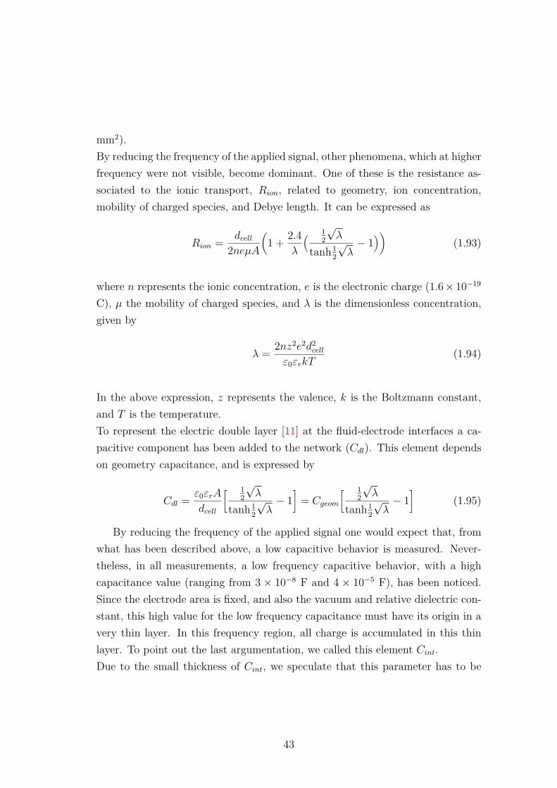
mm2).By reducing the frequency of the applied signal, other phenomena, which at higherfrequency were not visible, become dominant. One of these is the resistance as-sociated to the ionic transport, Rion, related to geometry, ion concentration,mobility of charged species, and Debye length. It can be expressed as

Rion = dcell2neµA

(1 + 2.4

λ

( 12

√λ

tanh12

√λ− 1

))(1.93)

where n represents the ionic concentration, e is the electronic charge (1.6× 10−19

C), µ the mobility of charged species, and λ is the dimensionless concentration,given by

λ = 2nz2e2d2cell

ε0εrkT(1.94)

In the above expression, z represents the valence, k is the Boltzmann constant,and T is the temperature.To represent the electric double layer [11] at the fluid-electrode interfaces a ca-pacitive component has been added to the network (Cdl). This element dependson geometry capacitance, and is expressed by

Cdl = ε0εrA

dcell

[ 12

√λ

tanh12

√λ− 1

]= Cgeom

[ 12

√λ

tanh12

√λ− 1

](1.95)

By reducing the frequency of the applied signal one would expect that, fromwhat has been described above, a low capacitive behavior is measured. Never-theless, in all measurements, a low frequency capacitive behavior, with a highcapacitance value (ranging from 3 × 10−8 F and 4 × 10−5 F), has been noticed.Since the electrode area is fixed, and also the vacuum and relative dielectric con-stant, this high value for the low frequency capacitance must have its origin in avery thin layer. In this frequency region, all charge is accumulated in this thinlayer. To point out the last argumentation, we called this element Cint.Due to the small thickness of Cint, we speculate that this parameter has to be

43

related to the Stern layer, which has typically a thickness of less than 1 nm. It istherefore possible to calculate the thickness of the Stern layer on each measure-ment using the following expression

Cstern[µF · cm−2] = Cint ·100A

(1.96)

dstern[nm] = 1Cintε0εrA

· 109 (1.97)

To ensure that Cint is charged at low frequency, however, a leakage resistivebranch which represents the motion of the charges towards the interface, chargingits thickness. This leakage process is represented in the model through the resistorRleak, which assumes very low values (between 100Ω and 103Ω).The physical meaning of this capacitive behavior at low frequency is still underinvestigation; several hypotheses have been advanced, the more promising is thatthis behavior is a consequence of adsorption processes occurring at the fluid-electrode interface, which justifies a relaxation at so low frequencies (mHz-Hz).

44

Chapter 2

Modeling

2.1 COMSOL Model

2.1.1 Introduction

A complete understanding of the physical picture associated to EIS and transientresults requires an agreement with simulations. COMSOL is a powerful interac-tive environment for modeling and solving all kinds of scientific and engineeringproblems based on partial differential equations. The software makes it possibleto extend conventional models for one type of physics into multiphysics mod-els that solve coupled physics phenomena simultaneously. The physics problemis written in one of three special syntaxes; (i) coeffcient form, (ii) general (orstrong) form, or (iii) weak form. In short, the coefficient form is for linear oralmost linear PDEs, the general form is for nonlinear PDEs, and the weak formoffers the maximum flexibility. When the problem is described in one of the threesyntaxes, COMSOL then internally compiles a set of PDEs representing the entiremodel. COMSOL uses the finite element method (FEM) and runs the finite ele-ment analysis together with adaptive meshing and error control using a varietyof numerical solvers. Consequently, one can easily define complex geometries inCOMSOL or solve problems where high precision is only required in some parts ofthe domain.

45

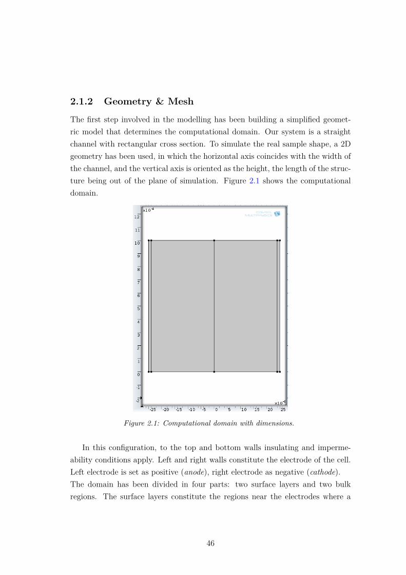
2.1.2 Geometry & Mesh

The first step involved in the modelling has been building a simplified geomet-ric model that determines the computational domain. Our system is a straightchannel with rectangular cross section. To simulate the real sample shape, a 2Dgeometry has been used, in which the horizontal axis coincides with the width ofthe channel, and the vertical axis is oriented as the height, the length of the struc-ture being out of the plane of simulation. Figure 2.1 shows the computationaldomain.

Figure 2.1: Computational domain with dimensions.

In this configuration, to the top and bottom walls insulating and imperme-ability conditions apply. Left and right walls constitute the electrode of the cell.Left electrode is set as positive (anode), right electrode as negative (cathode).The domain has been divided in four parts: two surface layers and two bulkregions. The surface layers constitute the regions near the electrodes where a

46

fine mesh is necessary to model the double-layer. The thickness of this layerdepends on ion concentration (λ); its value is fixed choosing the lowest between100 · dcell/

√λ and dcell/50.

An interface layer of 0.05 nm has been set at both left and right electrodes toaccount for the Stern layer.Once the geometry has been created, the next step is to build a mesh that isin agreement with the conflicting requirements of resolving relevant details suf-ficiently while keeping the computational costs in check. The main factors thatdetermine the mesh resolution are the characteristic length scales of the domaingeometry and of the relevant finest details.Given the fair regularity of our geometry, a so called "Mapping technique" hasbeen implemented to create a structured quadrilateral mesh on boundaries anddomains. This COMSOL node allows to control the number, size, and distributionof elements by using "Size" and "Distribution" subnodes. To create a mappedquadrilateral mesh for each domain, the mapped mesher maps a regular grid de-fined on a logical unit square onto each domain. The mapping method is based ontransfinite interpolation. The settings in the Size and Distribution features usedby the a Mapped feature determine the density of the logical meshes.The numberof mesh points in the bulk layer is 200, also in the surface layer it is 200. Thedistribution of mesh elements is fixed along the bulk regions, with 200 elements;left and right walls also has a fixed distribution with 2 elements. The mesh size inthe bulk is 0.12 µm. For the surface layers of the domain, an explicit exponentialdistribution of element sizes is used, with very fine elements near the electrodes.The element sizes in the domain range from a maximum of 0.12 × 10−6m to aminimum of 5.25× 10−11m.

2.1.3 Weak form implementation in COMSOL

The weak form is a particular way of specifying a model in COMSOL with amore general syntax. First, weak does not mean that the approach is inferior;weak form is very powerful and flexible. Weak form is a term borrowed frommathematics, but it has a slightly different meaning in this context. The strongpoints of the weak form that are relevant to this works is that it can (i) solve

47

strongly nonlinear problems, (ii) add and modify nonstandard constraints, and(iii) build models with PDEs on boundaries, edges and points. Furthermore, theweak solution form gives the exact Jacobian necessary for fast convergence ofstrongly nonlinear problems.

2.1.3.1 Derivation of the weak form

First, consider a general PDE problem for a single variable u defned on the 2Ddomain Ω with boundary ∂Ω in strong form

∂jΓij = Fi i = x, y, in Ω, (2.1)

where we use the Einstein summation notation. Let u(t) be an arbitrary functionon Ω called the test function (u(t) belongs to a suitable chosen, well-behaved classof functions). Multiplying the PDE with this function and integrating yields

∫Ωu(t)∂jΓijda =

∫Ωu(t)Fida (2.2)

We now use the Green’s theorem to integrate by parts

∫∂Ωu(t)(njΓij)ds−

∫Ω

[∂ju

(t)]Γijda =

∫Ωu(t)Fida (2.3)

This is rearranged to fit COMSOL syntax

0 = −∫∂Ωu(t)(njΓij)ds+

∫Ω

([∂ju

(t)]Γij + u(t)Fi

)da (2.4)

This is the weak reformulation of the original PDE. Note, the bulk divergenceterm ∂jΓij has been reduced to a (Neumann) boundary condition njΓij. One cansubstitute njΓij on the boundary where a (Neumann) boundary condition has tohold.The weak formulation is a weaker condition on the solution than the strong form

48

formulation. For instance, in the case of discontinuities in material properties, itis possible to find a solution in weak form while the strong form has no meaning.For this reason the weak form is used in numerical simulations. With the weakform comes the implementation of weak constraints which is the subject of thenext section.

2.1.4 Overview of COMSOL model equations

We review here the PDE problem implemented in the model. As stated in thefirst chapter ("Theoretical analysis"), the complete physical picture involves Mi-gration, Diffusion, Inflow and Outflow of ions, together with Auto-ionization andElectrolysis. What follows is a description of how each term has been imple-mented in COMSOL.

2.1.4.1 Ion concentration mass balance

• Migration & Diffusion

Nernst-Planck equation is a conservation of mass equation that describes themotion of chemical species in a fluid medium. It includes the flux of ions underthe influence of both an ionic concentration gradient ∇n and an electric fieldE = −∇V .

Jmig,diff = e∂n

∂t= e∇ ·

[D∇n+ Dze

kTn(∇V

)] [C

m3 · s

](2.5)

Where n is the concentration [m−3], e is the electric charge [C], D the diffusioncoefficient [m2 · s−1], z the valence, k the Boltzmann constant [J · K−1], T thetemperature [K], and V the applied voltage [V ]. For the reasons discussed inthe previous sections, the weak form of this equation has been implemented inCOMSOL. The chemical species include H+, OH−,

K+, Cl−, HCO−3 ; each of these species has its own NP equation, solved in theweak formulation.One issue is the extreme values of the concentration fields that can occur in

49

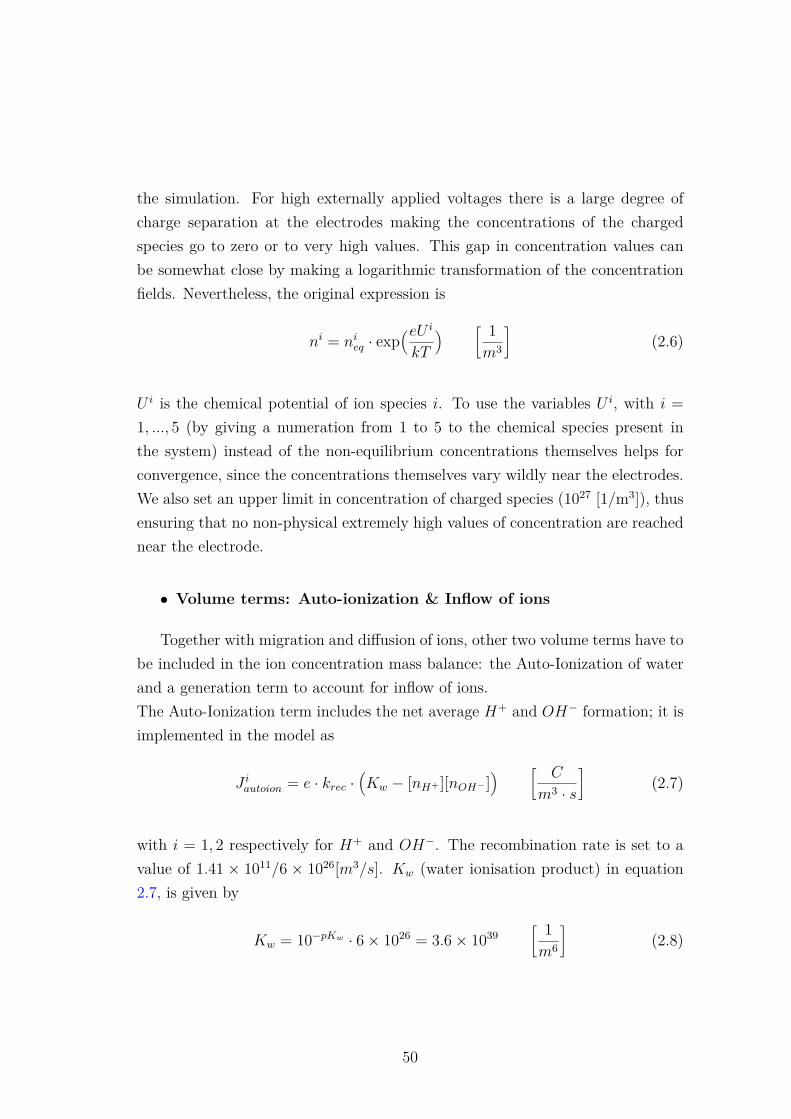
the simulation. For high externally applied voltages there is a large degree ofcharge separation at the electrodes making the concentrations of the chargedspecies go to zero or to very high values. This gap in concentration values canbe somewhat close by making a logarithmic transformation of the concentrationfields. Nevertheless, the original expression is

ni = nieq · exp(eU i

kT

) [ 1m3

](2.6)

U i is the chemical potential of ion species i. To use the variables U i, with i =1, ..., 5 (by giving a numeration from 1 to 5 to the chemical species present inthe system) instead of the non-equilibrium concentrations themselves helps forconvergence, since the concentrations themselves vary wildly near the electrodes.We also set an upper limit in concentration of charged species (1027 [1/m3]), thusensuring that no non-physical extremely high values of concentration are reachednear the electrode.

• Volume terms: Auto-ionization & Inflow of ions

Together with migration and diffusion of ions, other two volume terms have tobe included in the ion concentration mass balance: the Auto-Ionization of waterand a generation term to account for inflow of ions.The Auto-Ionization term includes the net average H+ and OH− formation; it isimplemented in the model as

J iautoion = e · krec ·(Kw − [nH+ ][nOH− ]

) [C

m3 · s

](2.7)

with i = 1, 2 respectively for H+ and OH−. The recombination rate is set to avalue of 1.41 × 1011/6 × 1026[m3/s]. Kw (water ionisation product) in equation2.7, is given by

Kw = 10−pKw · 6× 1026 = 3.6× 1039[ 1m6

](2.8)

50

where pKw = 14. Inflow of ions [m−3·s−1] is modeled through a volume generationterm; the net inflowing particle concentration of species i is then

Jinflow = e(nieq − ni) ·v

Lcell(2.9)

where v is the flow velocity (Poiseuille flow), and Lcell is the length of the channel;the quantity v

Lcellhas the unit of s−1 and is called residence time: time required

from an ion to flow from the inlet to the end of the channel.

• Boundary term: Electrolysis

The last process that has to be included in the overall ion concentration massbalance is the net H+ and OH− generation at left and right electrodes due toelectrolysis. This process is taken into account as a boundary condition.As already stated in the previous chapter, the current caused by injection of H+

and OH− at the electrodes has been modeled using the following relation

JH+

left = e · αgen · −∂V/∂x

V0/dcell

JH+

right = 0

JOH−

left = 0

JOH−

right = e · αgen ·∂V/∂x

V0/dcell(2.10)

All terms have the units of [C ·m−2 · s].To further improve the accuracy and thecloseness to reality of our model, expressions 2.10 should be replaced with theButler-Volmer equations for our system. The Butler-Volmer equation, as stated inprevious chapter, describes how the electrical current on an electrode depends on

51

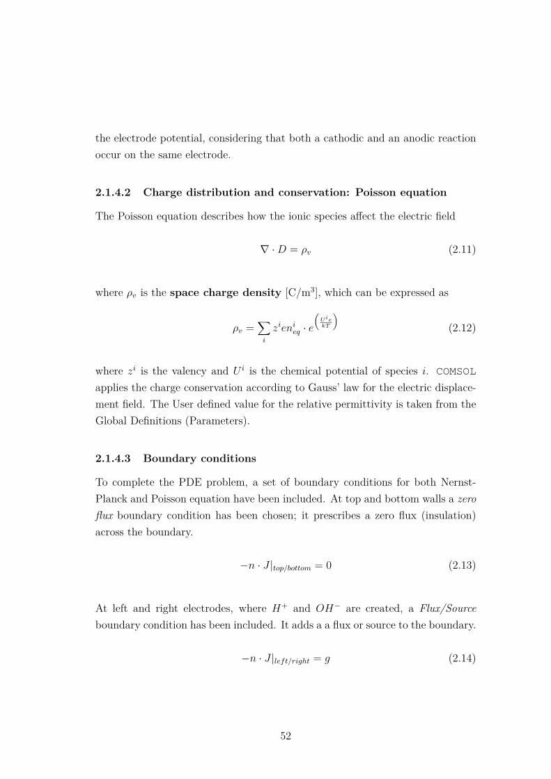
the electrode potential, considering that both a cathodic and an anodic reactionoccur on the same electrode.

2.1.4.2 Charge distribution and conservation: Poisson equation

The Poisson equation describes how the ionic species affect the electric field

∇ ·D = ρv (2.11)

where ρv is the space charge density [C/m3], which can be expressed as

ρv =∑i

zienieq · e(UiekT

)(2.12)

where zi is the valency and U i is the chemical potential of species i. COMSOL

applies the charge conservation according to Gauss’ law for the electric displace-ment field. The User defined value for the relative permittivity is taken from theGlobal Definitions (Parameters).

2.1.4.3 Boundary conditions

To complete the PDE problem, a set of boundary conditions for both Nernst-Planck and Poisson equation have been included. At top and bottom walls a zeroflux boundary condition has been chosen; it prescribes a zero flux (insulation)across the boundary.

−n · J |top/bottom = 0 (2.13)

At left and right electrodes, where H+ and OH− are created, a Flux/Sourceboundary condition has been included. It adds a a flux or source to the boundary.

−n · J |left/right = g (2.14)

52

where g is a source term, which in our case is coresponds to the injection current2.10.The charge conservation also includes a zero charge boundary condition whichapplies to both top and bottom walls. In COMSOL it is implemented through theZero Charge node, which adds a boundary condition that speficies zero charge onthe boundary.

−n ·D = 0 (2.15)

2.1.4.4 Calculation of current

The overall current that flows within the system can be calculated following twodifferent approaches. The first is from the electrode charge, the second is amethod which uses the Ramo-Shockley theorem to calculate the current. Havingtwo methods to calculate the measured current also increases, by comparing them,the reliability of result.

• Electrode charge

The first method to calculate the current is by taking into account the elec-trode charge.

I = dQel

dt=d(ε0εrLcellE

)dt

− αgen ·∂V/∂x

V0/dcell(2.16)

where V0 is the applied voltage, dcell is the cell gap, and Lcell is the length of thechannel.

• Ramo-Shockley

According to the Ramo-Shockley theorem [19; 20], each moving charged par-ticle contributes to the current on a chosen electrode in the following way

Iq = E0,vqv

∆V0(2.17)

53

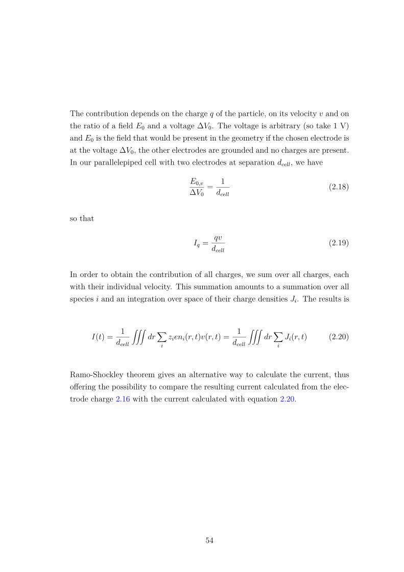
The contribution depends on the charge q of the particle, on its velocity v and onthe ratio of a field E0 and a voltage ∆V0. The voltage is arbitrary (so take 1 V)and E0 is the field that would be present in the geometry if the chosen electrode isat the voltage ∆V0, the other electrodes are grounded and no charges are present.In our parallelepiped cell with two electrodes at separation dcell, we have

E0,v

∆V0= 1dcell

(2.18)

so that

Iq = qv

dcell(2.19)

In order to obtain the contribution of all charges, we sum over all charges, eachwith their individual velocity. This summation amounts to a summation over allspecies i and an integration over space of their charge densities Ji. The results is

I(t) = 1dcell

∫∫∫dr∑i

zieni(r, t)v(r, t) = 1dcell

∫∫∫dr∑i

Ji(r, t) (2.20)

Ramo-Shockley theorem gives an alternative way to calculate the current, thusoffering the possibility to compare the resulting current calculated from the elec-trode charge 2.16 with the current calculated with equation 2.20.

54

Chapter 3

Experimental analysis

3.1 Introduction

To reproduce the theoretical results of the previous section, ideally, one would liketo probe the ionic concentration and electric field profiles inside a microdevice.Unfortunately, that is not feasible, but other quantities can be measured (e.g.transient current flowing towards an electrode or the frequency response of com-plex electric impedance); and then these can be correlated to the electrochemicalparameters of interest.

Electrical characterization of electrophoretic microcells, micro-channel con-taining electrolyte solutions, and a lot of other electrochemical devices, is oftenperformed by means of two experimental techniques: Electrochemical ImpedanceSpectroscopy (EIS) and Potential Step Voltammetry also referred to astransient current measurements. The former probes the frequency response ofthe system by applying a small amplitude sinusoidal voltage (50 mV); the latterstudies the current flowing into a given device as a function of time, typically fora time window of about 102 s.

Our purpose is to characterize a set of microfluidic devices containing elec-trolyte solutions. All of them are straight microchannels with a rectangular sec-tion. They differ in dimensions and materials. Two of the walls of the channel

55

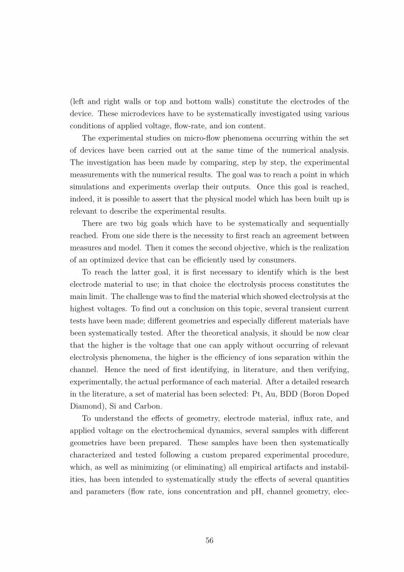
(left and right walls or top and bottom walls) constitute the electrodes of thedevice. These microdevices have to be systematically investigated using variousconditions of applied voltage, flow-rate, and ion content.

The experimental studies on micro-flow phenomena occurring within the setof devices have been carried out at the same time of the numerical analysis.The investigation has been made by comparing, step by step, the experimentalmeasurements with the numerical results. The goal was to reach a point in whichsimulations and experiments overlap their outputs. Once this goal is reached,indeed, it is possible to assert that the physical model which has been built up isrelevant to describe the experimental results.

There are two big goals which have to be systematically and sequentiallyreached. From one side there is the necessity to first reach an agreement betweenmeasures and model. Then it comes the second objective, which is the realizationof an optimized device that can be efficiently used by consumers.

To reach the latter goal, it is first necessary to identify which is the bestelectrode material to use; in that choice the electrolysis process constitutes themain limit. The challenge was to find the material which showed electrolysis at thehighest voltages. To find out a conclusion on this topic, several transient currenttests have been made; different geometries and especially different materials havebeen systematically tested. After the theoretical analysis, it should be now clearthat the higher is the voltage that one can apply without occurring of relevantelectrolysis phenomena, the higher is the efficiency of ions separation within thechannel. Hence the need of first identifying, in literature, and then verifying,experimentally, the actual performance of each material. After a detailed researchin the literature, a set of material has been selected: Pt, Au, BDD (Boron DopedDiamond), Si and Carbon.

To understand the effects of geometry, electrode material, influx rate, andapplied voltage on the electrochemical dynamics, several samples with differentgeometries have been prepared. These samples have been then systematicallycharacterized and tested following a custom prepared experimental procedure,which, as well as minimizing (or eliminating) all empirical artifacts and instabil-ities, has been intended to systematically study the effects of several quantitiesand parameters (flow rate, ions concentration and pH, channel geometry, elec-

56

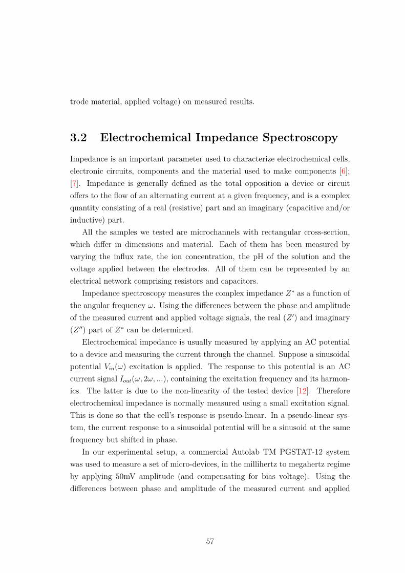
trode material, applied voltage) on measured results.

3.2 Electrochemical Impedance Spectroscopy

Impedance is an important parameter used to characterize electrochemical cells,electronic circuits, components and the material used to make components [6];[7]. Impedance is generally defined as the total opposition a device or circuitoffers to the flow of an alternating current at a given frequency, and is a complexquantity consisting of a real (resistive) part and an imaginary (capacitive and/orinductive) part.

All the samples we tested are microchannels with rectangular cross-section,which differ in dimensions and material. Each of them has been measured byvarying the influx rate, the ion concentration, the pH of the solution and thevoltage applied between the electrodes. All of them can be represented by anelectrical network comprising resistors and capacitors.

Impedance spectroscopy measures the complex impedance Z∗ as a function ofthe angular frequency ω. Using the differences between the phase and amplitudeof the measured current and applied voltage signals, the real (Z ′) and imaginary(Z ′′) part of Z∗ can be determined.

Electrochemical impedance is usually measured by applying an AC potentialto a device and measuring the current through the channel. Suppose a sinusoidalpotential Vin(ω) excitation is applied. The response to this potential is an ACcurrent signal Iout(ω, 2ω, ...), containing the excitation frequency and its harmon-ics. The latter is due to the non-linearity of the tested device [12]. Thereforeelectrochemical impedance is normally measured using a small excitation signal.This is done so that the cell’s response is pseudo-linear. In a pseudo-linear sys-tem, the current response to a sinusoidal potential will be a sinusoid at the samefrequency but shifted in phase.

In our experimental setup, a commercial Autolab TM PGSTAT-12 systemwas used to measure a set of micro-devices, in the millihertz to megahertz regimeby applying 50mV amplitude (and compensating for bias voltage). Using thedifferences between phase and amplitude of the measured current and applied

57

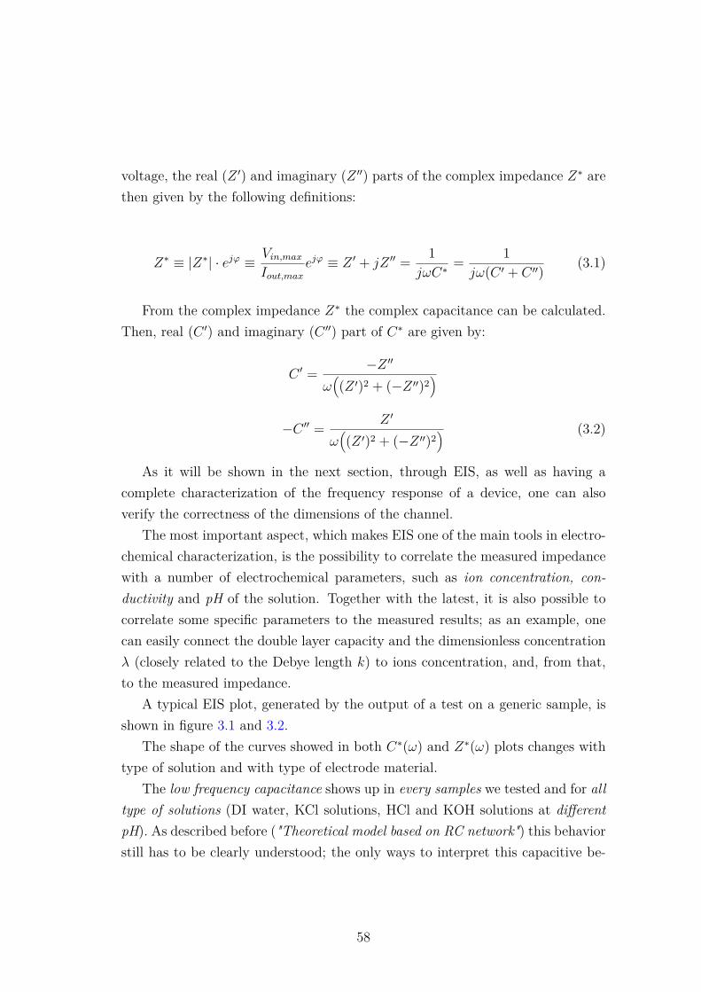
voltage, the real (Z ′) and imaginary (Z ′′) parts of the complex impedance Z∗ arethen given by the following definitions:

Z∗ ≡ |Z∗| · ejϕ ≡ Vin,maxIout,max

ejϕ ≡ Z ′ + jZ ′′ = 1jωC∗

= 1jω(C ′ + C ′′) (3.1)

From the complex impedance Z∗ the complex capacitance can be calculated.Then, real (C ′) and imaginary (C ′′) part of C∗ are given by:

C ′ = −Z ′′

ω((Z ′)2 + (−Z ′′)2

)

−C ′′ = Z ′

ω((Z ′)2 + (−Z ′′)2

) (3.2)

As it will be shown in the next section, through EIS, as well as having acomplete characterization of the frequency response of a device, one can alsoverify the correctness of the dimensions of the channel.

The most important aspect, which makes EIS one of the main tools in electro-chemical characterization, is the possibility to correlate the measured impedancewith a number of electrochemical parameters, such as ion concentration, con-ductivity and pH of the solution. Together with the latest, it is also possible tocorrelate some specific parameters to the measured results; as an example, onecan easily connect the double layer capacity and the dimensionless concentrationλ (closely related to the Debye length k) to ions concentration, and, from that,to the measured impedance.

A typical EIS plot, generated by the output of a test on a generic sample, isshown in figure 3.1 and 3.2.

The shape of the curves showed in both C∗(ω) and Z∗(ω) plots changes withtype of solution and with type of electrode material.

The low frequency capacitance shows up in every samples we tested and for alltype of solutions (DI water, KCl solutions, HCl and KOH solutions at differentpH). As described before ("Theoretical model based on RC network") this behaviorstill has to be clearly understood; the only ways to interpret this capacitive be-

58

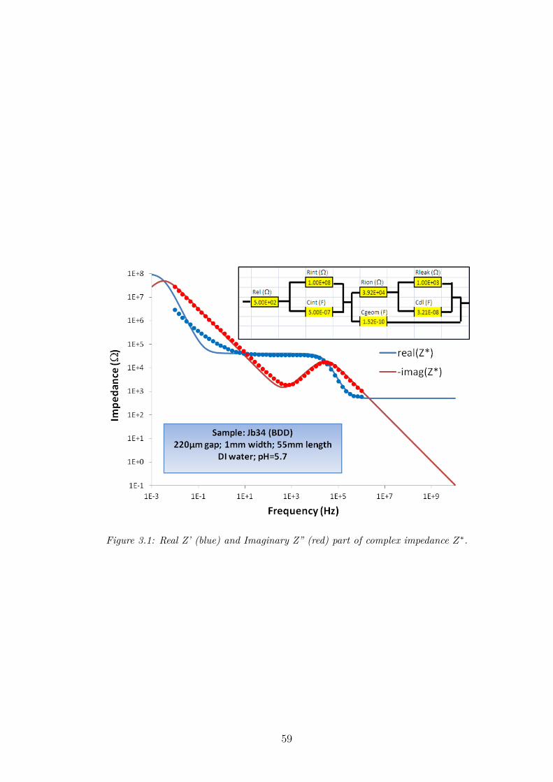
Figure 3.1: Real Z’ (blue) and Imaginary Z” (red) part of complex impedance Z∗.

59

Figure 3.2: Real C’ (blue) and Imaginary C” (red) part of complex capacitance C∗.

60

havior is by making some hypothesis on its origin, and test them experimentally.The physical interpretation we speculate is a charge accumulation mechanism,

in a very small thickness, at the interface between electrode and solution. Weverified whether this process is flux dependent or not; indeed, as it will be de-scribed later ("Measuring protocol"), also tests with reduced flux and even withoutflux have been performed. The results of the tests without flow have been thencompared to the results of the tests with flow. The results of EIS experimentsshow that no significant variations of the low frequency capacitance with flow arepresent.

3.3 Potential Step Voltammetry

Experimentally the ionic fluxes can be determined from the electrical transientcurrent that flows externally between the electrodes after a voltage is applied[? ]. This technique involves the application of a potential step to an electrodepair, and is based on the measure of the current caused by the applied voltagein a fixed time window, typically between 100s and 200s. Typically a series ofdifferent voltages is used and, for each amplitude, both polarities are sequentiallyapplied. In this way, any accumulation of charges of the same polarity on thewalls of the device, which would alter the simmetry and could affect the stabilityfor long periods, can be avoided.

All current traces start from equilibrium (no voltage applied for a sufficientlylong period of time) and step towards values between 100 mV and 3-5 V, depend-ing on electrodes material. An illustration of the time variation of the appliedvoltage is given in figure 3.3.

For each voltage V, a sequence of "regimes" is followed, which we will call0 −→ V , V −→ 0, 0 −→ −V and −V −→ 0. Here a sample time of 100 s is usedtogether with a zero volt multiplier equal to 2 which means that the V −→ 0 andthe −V −→ 0 regimes are applied 2 times longer than the 0 −→ V and 0 −→ −Vregimes. This allows the sample to sufficiently relax back to its equilibrium state.

The measurement setup is controlled through a custom written Labview pro-gram. It allows among other things to set the sample time (s), the scan rate

61

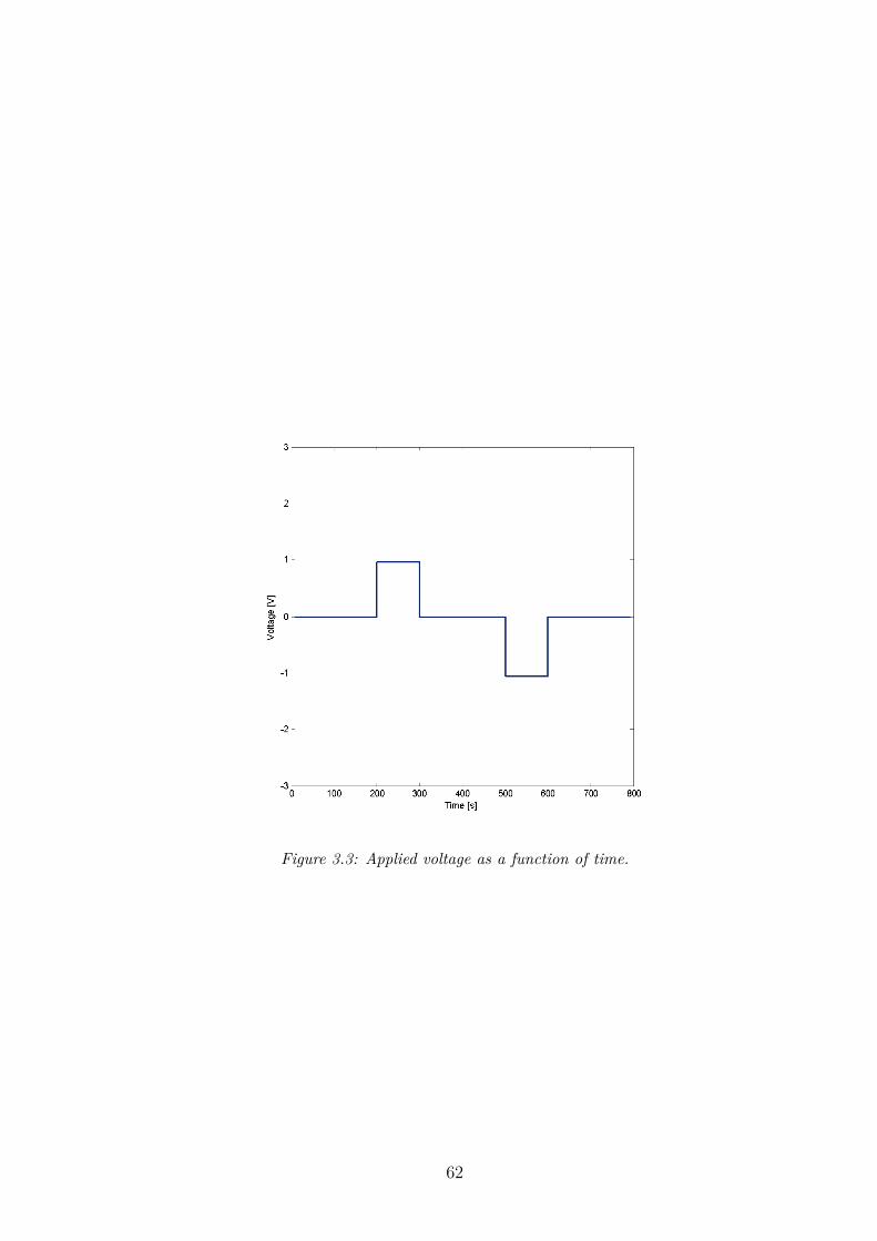
Figure 3.3: Applied voltage as a function of time.

62

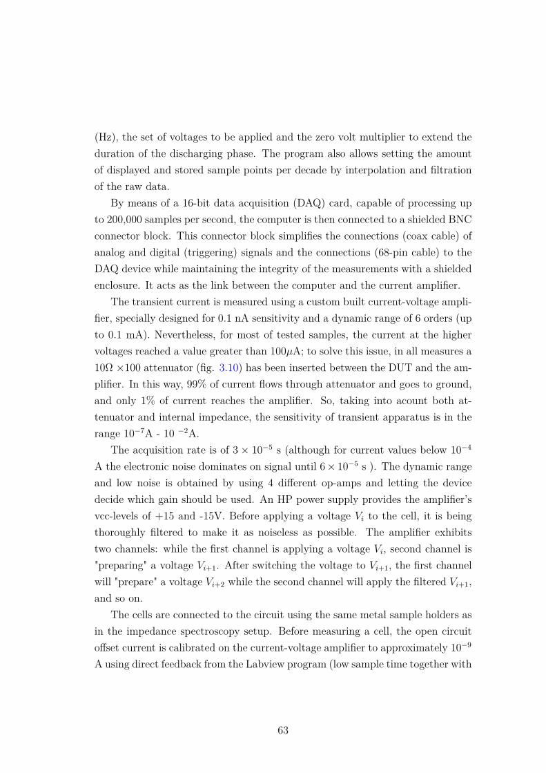
(Hz), the set of voltages to be applied and the zero volt multiplier to extend theduration of the discharging phase. The program also allows setting the amountof displayed and stored sample points per decade by interpolation and filtrationof the raw data.

By means of a 16-bit data acquisition (DAQ) card, capable of processing upto 200,000 samples per second, the computer is then connected to a shielded BNCconnector block. This connector block simplifies the connections (coax cable) ofanalog and digital (triggering) signals and the connections (68-pin cable) to theDAQ device while maintaining the integrity of the measurements with a shieldedenclosure. It acts as the link between the computer and the current amplifier.

The transient current is measured using a custom built current-voltage ampli-fier, specially designed for 0.1 nA sensitivity and a dynamic range of 6 orders (upto 0.1 mA). Nevertheless, for most of tested samples, the current at the highervoltages reached a value greater than 100µA; to solve this issue, in all measures a10Ω ×100 attenuator (fig. 3.10) has been inserted between the DUT and the am-plifier. In this way, 99% of current flows through attenuator and goes to ground,and only 1% of current reaches the amplifier. So, taking into acount both at-tenuator and internal impedance, the sensitivity of transient apparatus is in therange 10−7A - 10 −2A.

The acquisition rate is of 3× 10−5 s (although for current values below 10−4

A the electronic noise dominates on signal until 6× 10−5 s ). The dynamic rangeand low noise is obtained by using 4 different op-amps and letting the devicedecide which gain should be used. An HP power supply provides the amplifier’svcc-levels of +15 and -15V. Before applying a voltage Vi to the cell, it is beingthoroughly filtered to make it as noiseless as possible. The amplifier exhibitstwo channels: while the first channel is applying a voltage Vi, second channel is"preparing" a voltage Vi+1. After switching the voltage to Vi+1, the first channelwill "prepare" a voltage Vi+2 while the second channel will apply the filtered Vi+1,and so on.

The cells are connected to the circuit using the same metal sample holders asin the impedance spectroscopy setup. Before measuring a cell, the open circuitoffset current is calibrated on the current-voltage amplifier to approximately 10−9

A using direct feedback from the Labview program (low sample time together with

63

high frequency). After completing the voltage sequence, the measurements arewritten to a text-file which is later on imported in Excel for post-processing.

The first applied voltage is zero. The corresponding measured current is equalto the offset current which will be subtracted from the voltage curves.

One issue is related to the sensitivity of the offset current to Room Temper-ature variations. Since it takes almost 3 hours to obtain a complete series ofvoltages (600s per each amplitude; 17 different amplitudes), room temperaturecan easily drift within this time window (especially in early morning and lateevening); typically the drift is between 21’C and 25’C (in summer).

To understand and quantify this effect, a long weekend measure at 0V (ac-quired using linear filtering) has been conducted, by simply leaving the metalsample holders disconnected into the closed Faraday cover. At the same time theroom temperature has been recorded through the temperature meter (Voltcraft),which is equipped with software that can be used to download the measured dataon hard disk.

The result of this test is shown in figure 3.4.To quantify the dependence of offset current from room temperature, a I-T

plot is useful (Figure 3.5). The rate of change for the offset with room temperatureis approximately 2nA·C−1. The offset current dependence with room temperaturebecomes visible in a complete series of voltage step measures, and manifests itselfas a spread in the last acquired current values in the discharging phase at differentvoltage amplitudes.

One aspect that makes transient current measurements very useful for ourpurpose is that from its output it is possible to estimate and study the transportphenomena occurring within the channel. Indeed, a movement of charged speciesis associated to a current flowing towards the electrodes. By observing the be-havior of the measured I-t curve, it is possible to establish which mechanism islimiting the transport.

Obviously the shape of the measured curve strongly depends from which so-lution is flowing into the channel. Solutions with lower ions content will also havelower values of the measured current; so, the transient current typically increasesby moving from DI water to 3ppm, and will increase more by moving to higherconcentration (30ppm or even 300ppm).

64

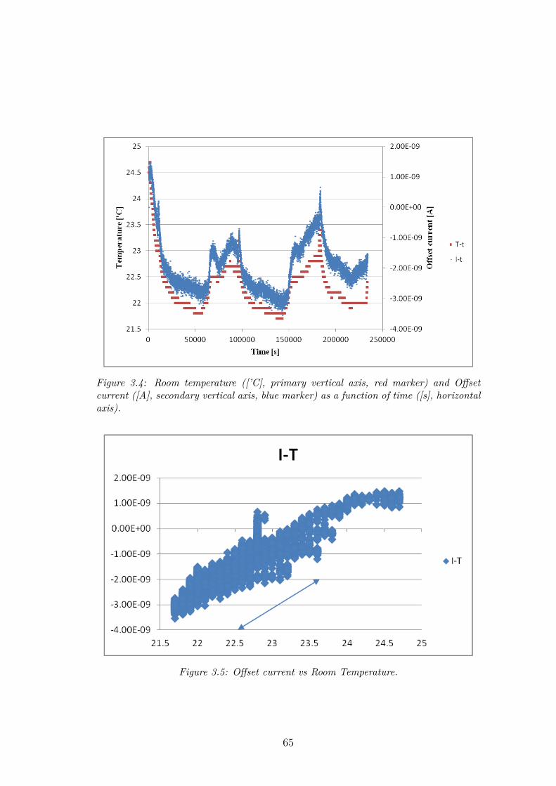
Figure 3.4: Room temperature ([’C], primary vertical axis, red marker) and Offsetcurrent ([A], secondary vertical axis, blue marker) as a function of time ([s], horizontalaxis).

Figure 3.5: Offset current vs Room Temperature.

65

3.3.1 I-t plot

Let’s see how an I-t plot with a solution containing 30 or 300ppm of KCl can beinterpreted.

3.3.1.1 Transient regime

When a voltage of sufficient amplitude (high enough to completely separate ionsand low enough not to be in the exponential electrolysis regime) is suddenly ap-plied (for a given geometry and concentration), all ions start to migrate towardsopposite charged electrodes; this process reflects itself as a measured current. So,in the transient regime, the higher the concentration, the higher will be the mea-sured current. The regime that will be established strongly depends on appliedvoltage’s amplitude. For lower voltages, as described analytically in [4], the sep-aration effect doesn’t show up. For sufficient voltage amplitudes (zeV > 10kT )and ions concentration (2(zed)2n

ε0εrkT< 20exp(1

4zeVkT

)) the "separated n" regime willbe established. As stated in the first chapter, for a microdevice a voltage of1V is sufficient to establish the separation regime (for macroscale devices 5V).The required time for an ion to migrate towards the opposite charged electrodeis determined by its mobility. Since K+ and Cl− have almost same mobilities,they will reach the opposite charged electrodes almost at the same time. Thissymmetry doesn’t apply for H+ and OH− ions. Indeed, the mobility of H+ is3.6× 10−7m2V −1s−1, and for OH− is 2× 10−7m2V −1s−1, so, H+ ions are ' 2×faster than OH−. This also mean that the recombination point of H+ and OH−ions will not be in the center of the channel, but, due to the different mobilities,it will be closer to the negatively charged electrode.

3.3.1.2 Transition from transient to Steady-State

If no other process (flow, autoionization, injection) acts, once all ions have mi-grated towards opposite charge electrodes, the center of the channel becomesempty of charged species, and then the measured current would decrease to zero.In a real experiment, however, all other previously described phenomena con-tributing to current are present.

66

The convective flow acts as a reservoir of ions. The amount of fluid com-ing from an upstream cross section, indeed, is rich in new ions, since it hasn’texperimented any applied voltage yet.

As previously described, the flow profile is parabolic (Poiseuille), so the ve-locity will be higher in the center, and will decrease with quadratic law to "zero"moving towards the channel walls. This feature generates an accumulation of ionsat the sides of the channel, meaning that the ions concentration inside the vol-ume where the voltage is applied increases in time. A typical I-t test has a timewindow of 100s. Within this time, the accumulation of ions at the electrodesis such relevant that, at some point (end of transient regime and beginning ofsteady-state), they build up achieving a concentration able to screens the electricfield in the center of the channel. Once the electric field is screened, K+ and Cl−

ions don’t contribute anymore to measured current.Now, if nothing else acts to give contribution to current, the steady-state

current would decrease to zero. Nevertheless, two coupled processes result in ameasured current: the injection of H+ and OH− at the electrodes, whichgenerates a new amount of additional charged species, and their recombina-tion in the bulk. H+ and OH− ions generated at electrodes experiment theelectric field generated from the applied voltage, and will migrate towards oppo-site charged electrode, thus giving a new contribute to the measured current. Inthis process, also diffusion acts a in the same direction of migration, being theconcentration of H+ and OH− higher at their generation point.

H+ and OH− ions generated at the electrodes are then transported both bymigration and diffusion from the sides toward the center where, due to autoion-ization, they react to recombine and form H2O.

The steady-state current is mainly determined by two mechanisms which actsimultaneously and balance each other: migration and diffusion of H+ and OH−ions generated from reactions at the electrodes and their recombination due toautoionization in the bulk.

When applied voltage overcomes the threshold required to generate H2 andO2 at electrodes, new additional charges will be created, and so the measuredcurrent will increase its value. Electrolysis is very easy to be individuated inan I-V plot (usually reported with the last acquired points), since, when the

67

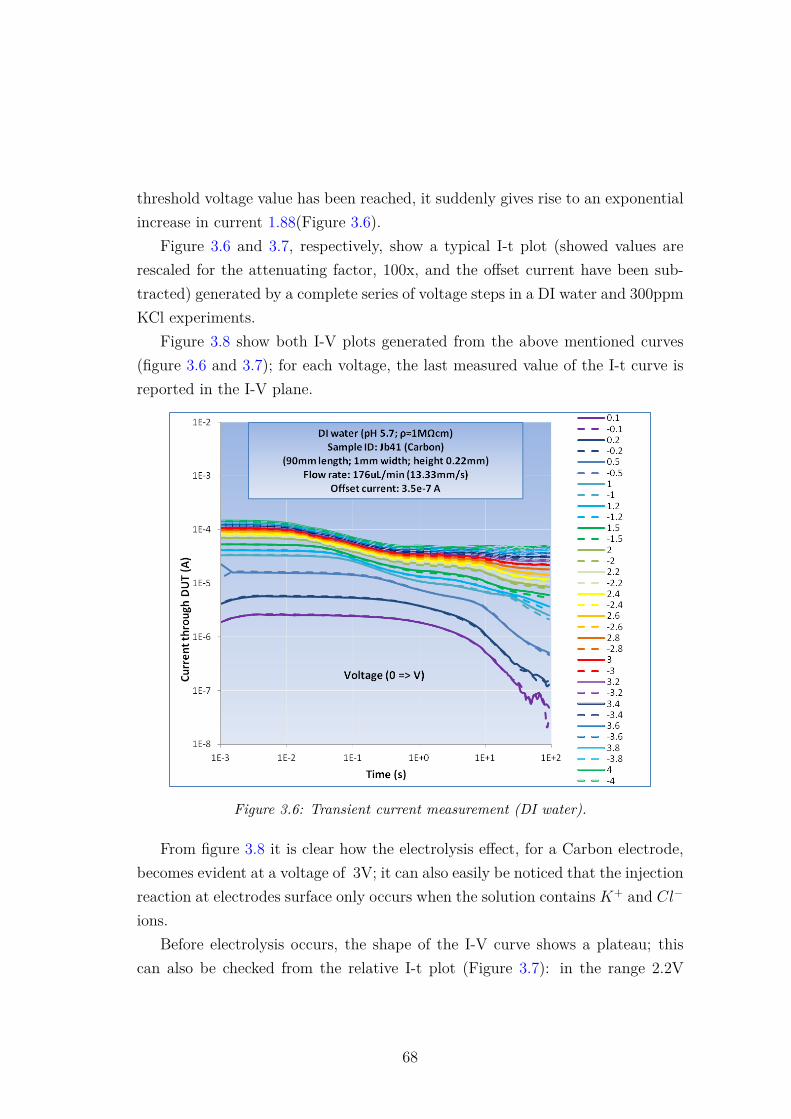
threshold voltage value has been reached, it suddenly gives rise to an exponentialincrease in current 1.88(Figure 3.6).

Figure 3.6 and 3.7, respectively, show a typical I-t plot (showed values arerescaled for the attenuating factor, 100x, and the offset current have been sub-tracted) generated by a complete series of voltage steps in a DI water and 300ppmKCl experiments.

Figure 3.8 show both I-V plots generated from the above mentioned curves(figure 3.6 and 3.7); for each voltage, the last measured value of the I-t curve isreported in the I-V plane.

Figure 3.6: Transient current measurement (DI water).

From figure 3.8 it is clear how the electrolysis effect, for a Carbon electrode,becomes evident at a voltage of 3V; it can also easily be noticed that the injectionreaction at electrodes surface only occurs when the solution contains K+ and Cl−

ions.Before electrolysis occurs, the shape of the I-V curve shows a plateau; this

can also be checked from the relative I-t plot (Figure 3.7): in the range 2.2V

68

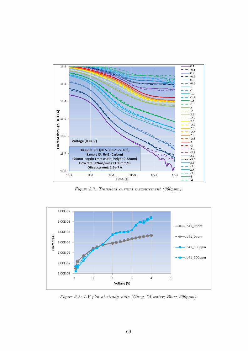
Figure 3.7: Transient current measurement (300ppm).

Figure 3.8: I-V plot at steady state (Grey: DI water; Blue: 300ppm).

69

to 2.8V all the curves end with the same steady state current. Then, when theelectrolysis threshold voltage is reached, the strong increase in current is due toreactions at electrodes.

3.4 Experimental Setup

3.4.1 Measuring block

EIS measures have been carried out through a very wide dynamic range (mHz-MHz) commercial Autolab TM PGSTAT-12. The potential amplitude of thesignal is of 50 mV. The supply for the Autolab apparatus comes directly fromthe network. The output, or the signal to be applied to the sample, is connectedto the electrodes through an amplifier. The hardware is controlled by the Novasoftware, interfaced by USB connection to the terminal. The graphical interfaceof the software, while measuring, appears as in figure 3.9. The possibility ofchecking the amplitude and the phase of measured signal during the experimentand the live updating of Nyquist –Z” vs Z’ plot, constitutes two very useful toolsthrough which control and follow the trend of a measure.

A four channels scope (Tektronix TDS3034B) is connected to the AutolabPGSTAT12; in this way it is possible to check the voltage signal applied to thesample. Through the scope one can check both the wave form of the appliedvoltage signal and of the measured current. This device is indispensable to havea direct feedback on how the system is responding to the external stimulus (volt-age).

To do the Voltammetry tests a 100x 10Ω attenuator has been interposedbetween the amplifier and the sample. With this trick the current generatedby the higher amplitude voltage steps, which often overcome the 100 µA upperlimit of apparatus sensitivity, can be recorded. The attenuator has a very simpleconfiguration, reported in figure 3.10. The custom built amplifier, as previouslydescribed, has a sensitivity of 10−7A (considering the 10Ω× 100 attenuator andthe amplifier internal impedance of 1 kΩ), an acquisition speed of a 30 to 60µs (depending on current amplitude), and 6 orders wide dynamic range (up to

70

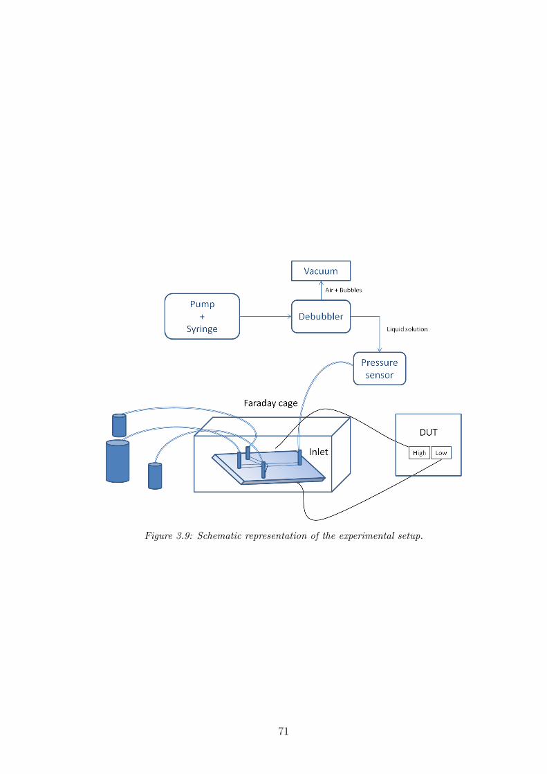
Figure 3.9: Schematic representation of the experimental setup.

71

mA). The initial current flowing (mA in a few µs) is responsible of charging thecapacitor, and is intentionally left out of the measuring plot.

Figure 3.10: 10 Ω(100x) attenuator’s scheme.

3.4.2 Room temperature meter

The room temperature meter is a Voltcraft DL-140TH. This temperature andhumidity data logger is intended to be used for monitoring and collecting dataof environment temperature and humidity. It has been used to monitor andcollect temperature and humidity values efficiently and conveniently for long timeperiods. The readings are saved in the logger and simply read out by PC witha USB port. The LCD can show current readings, MAX, MIN, TIME, DATEand temperature or humidity values. The data logger is designed with a highaccuracy temperature and humidity sensor with fast response and stability.

72

Figure 3.11: Temperature datalogger.

3.4.3 Pressure sensor

The pressure sensor has been placed between the debubbler and the sample. Thesupply is given by a 10 V Delta Elektronika (ES015-10) power supplier. Thepressure transducer implements a conversion of the pressure signal into a voltagesignal. The latter is then read and processed by a multimeter, which shows themeasured value (mV) on its display. The system is calibrated such that 50 mVcorresponds to 1 bar.

Checking the pressure within the channel is crucial. A second aspect whichmakes this element more useful is the possibility to know, at each time, whichis the velocity within the channel. All tested samples are straight channels withrectangular cross section; once the influx rate is fixed, one can easily obtain thevelocity within the channel by simply multiplying this quantity for the crosssection. By knowing the velocity, the length of the channel, and the viscosity ofthe fluid, it is possible to obtain the theoretical pressure drop. The exact valueis not possible to obtain; indeed, to know this quantity, one should know theanalytic solution for the Poiseuille problem in a rectangular cross section. Thissolution is nowadays unknown. To obtain an approximate value there are severaloptions, one of this is by representing the solution as a expansion in Fourier terms.

The Navier-Stokes problem, for this geometry, is expressed by

[∂2y + ∂2

z ]vx(y, z) = −∆pµL

− 12w < y <

12w, 0 < z < h

73

vx(y, z) = 0 y = ±12w, z = 0, z = h (3.3)

where h is the height of the channel, w the width, L the length. In theprevious relations it has been adopted an orthonormal reference where x is in thedirection of the length of the channel, y axes is directed as its width, and z axesas its height.

The no slip boundary condition is expressed by

vx(y, 0) = 0vx(y, h) = 0 (3.4)

To fulfill this condition only terms proportional to sin(nπzh−1) have to betaken into account in the Fourier expansion, where n is a positive integer.

After some calculations, not reported here, an expression for the influx rateQ can be obtained,

Q ' h3w∆p12µL

[1−

inf∑n,odd

1n5

192π5

h

wtanh

(nπ

w

2h)]

(3.5)

from this expression one can calculate the pressure drop within the channel.The value obtained through the last expression has been taken as a reference

to test if the pressure sensor was working as it should. The comparison betweenthe latter and the measured value showed a good agreement.

The estimated value for the pressure within the channel has constituted areference with which testing the sensor first, and then a tool through whichcalculating the influx rate that had to be set, for each sample, to obtain a velocitywithin the channel of 13.33 mm/s. Indeed, to make all tests on different samplescomparable each other, the influx rate was set such that the velocity within thechannel was 13.33 mm/s. In this way, for each sample, once the influx rategenerating a velocity of 13.33mm/s was known, the theoretical value for thepressure within the channel has been calculated. Then a comparison between thelatter and the value showed by the sensor is has been possible to know whetherthe pressure within the channel was the expected one.

Working following the last procedure also ensured that the tubing tightnessand connections system have been optimized.

74

Some samples have very small dimensions (h=5µm, w=100µm), so also anon-perfect mechanic coupling could generate a leakage, or a pressure drop. Bymonitoring the pressure through the sensor one can be sure that these leakagesare noticed and corrected.

3.4.4 Conductivity meter & cell

The conductivity meter is composed of a CDM210 MeterLabTM apparatus con-nected to a Radiometer analytic CDC641T conductivity cell with temperaturesensor. The latter has a 2-pole universal conductivity electrode with glass bodyand temperature sensor (Max. temperature 100’C, min. immersion depth 14 mm,cell constant 0.85 ≤ 0.87 ≤ 1.15 cm−1); it has a traditional design based on twoplates of platinum, and is ideal for routine measurement of conductivity and foruse with a sample changer due to the easy rinsing. Conductivity measurementis temperature dependent (if the temperature increases so does the conductivityvalue), this is the reason why a cell with a built-in temperature sensor (set at 25’Cas a reference and with a correction coefficient of 2%

′C) was chosen. Conductivity

can be corrected to a reference temperature of 20 or 25’C. Sample temperaturescan be measured automatically or entered manually.

Some of the features available on the CDM210 are the automatic frequencyswitching, the AUTOREAD function, and, most importantly, high precision mea-surements: conductivity measurements in the range 0.001 µS/cm to 5.99 S/cmand resistivity measurements in the range 0.2 Ω·cm to 1.0 GΩ·cm.

3.4.5 pH meter

The pH meter is an IQ160G-KIT Bluetooth Waterproof Handheld (-2.00 to 19.99range, ± 0.01 pH of accuracy). The stainless steel pH probe has a virtuallyunbreakable sensor that stores dry and needs no maintenance, thereby eliminatingthe frustrations of using delicate glass electrodes. To calibrate the probe, we beginwith pH 7 buffer, then moved to the second buffer (pH 4) and finally to additionalbuffers.

Notably measuring the pH of DI water takes a long time. To measure the pH

75

of DI water, it has been used the following trick: adding a very small amountof NaCl to the solution, so that the pH value is not altered but the probe of itsvalue is much faster.

Also this sensor is temperature compensated, although the variation is lessimportant than for the conductivity measurements. By having two probes, bothof them temperature compensated, showing the actual solution temperature, itis possible to compare their output and verify if the measured values match.

3.4.6 Pump and syringes

The pumping system includes a syringe, hosting the fluid, and a pump, whichprovides the mechanic energy needed to forward through the sample.

The pump, an Harvard Apparatus (11plus), has to be calibrated with thesyringe used for the experiment; what has to be done is setting the diameter ofthe syringe to calibrate the rotation of the pump.

Tested samples have very different dimensions, so syringes with different vol-umes (from 2.5 ml to 60 ml) have been used. Every time the syringe has beenchanged, a reconfiguration of the pump by updating the diameter has been nec-essary.

3.4.7 Debubbler/Degasser

The device we used (Systec Degasser/Debubblers 9000-1544) has a total volumeof 5mL. The bubbles elimination module is based on gravity. Removing of bothbubbles and dissolved gases from the flow path improves dispense precision andaccuracy and enhances overall system performance. By combining vacuum de-gassing with active bubble removal, the Systec Degasser/Debubblers both elim-inate existing bubbles and actually prevent the formation of new bubbles byremoving the dissolved gases before they can nucleate and cause problems.

76

3.4.8 Sample stage

The sample to test is placed into a Faraday cage, so that parasitic effects comingfrom surroundings are reduced.

The connection is made via two terminals (positive and negative) which areconnected to the electrode pair of the sample. For the impedance measurementsalso a grounding cable was needed.

Figure 3.12 gives an idea of how the experimental setup looks like.

3.5 Experimental setup validation

Before running experiments on true samples, it is necessary to test and verifythe reliability of both the Electrochemical Impedance Spectroscopy (EIS) andthe Potential Step Voltammetry (or Transient Current Measurements) setups.Indeed, to achieve a reliable result, one has to be sure that the system throughwhich the quantity object of the study is measured is working in a correct wayand with as less artifacts as possible. Also, it has to be ensured that the outputof the measures constitutes a reliable basis on which building a theoretical model.Typically this test is carried out by measuring known quantities, such as simpleand known electrical networks, and by comparing the expected values with themeasured one.

It is convenient to use as a reference circuit a simple R(RC) network; thereason that justifies this choice is that this circuit also well represents the typicalresponse of a true sample, so it can also be used as a reference through which fitsthe measured data.

The electrical circuit is showed in figure 3.13.With the following expected values for the elements:

RS=120 Ω ; RP=150k Ω ; CP=200 µF

The voltage drop can be expressed as

U = (RS +RP )I −RP IC (3.6)

77

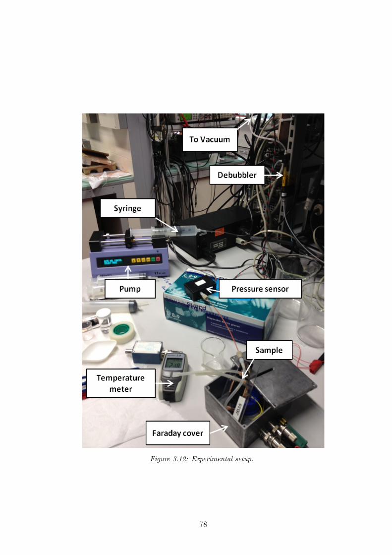
Figure 3.12: Experimental setup.

78

Figure 3.13: RRC reference circuit used to validate both EIS and Voltammetry appara-tus.

From this expression one can easily obtain the total current flowing throughthe network

I = U +RP ICRSRP

(3.7)

And, for the voltage drop through the capacitor,

QC

C= RP

(I − IC

)(3.8)

One can assume that the voltage drop U is constant. Then, by expressingIC from eq.3.7 and substituting the expression for I given by eq. 3.8, we obtain(U=const)

IC = U

RS

− RS +RP

RSRP

QC

C(3.9)

The expression for the time dependence of IC is then

IC = U

RS

e−tRS+RP

RSRPC (3.10)

From which, by integrating from t0 = 0 to time t, one can obtain the chargeaccumulated during time in the capacitor as

QC = URPC

RS +RP

(1− e−t

RS+RPRSRPC

)(3.11)

79

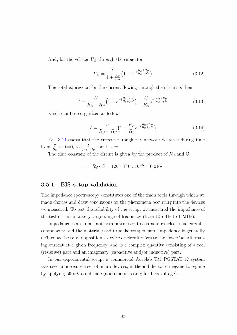
And, for the voltage UC through the capacitor

UC = U

1 + RSRP

(1− e−t

RS+RPRSRPC

)(3.12)

The total expression for the current flowing through the circuit is then

I = U

RS +RP

(1− e−t

RS+RPRSRPC

)+ U

RS

e−tRS+RP

RSRPC (3.13)

which can be reorganized as follow

I = U

RS +RP

(1 + RP

RS

e−tRS+RP

RSRPC

)(3.14)

Eq. 3.14 states that the current through the network decrease during timefrom U

RSat t=0, to U

(RS+RP ) , at t−→∞.The time constant of the circuit is given by the product of RS and C

τ = RS · C = 120 · 180× 10−6 = 0.216s

3.5.1 EIS setup validation

The impedance spectroscopy constitutes one of the main tools through which wemade choices and draw conclusions on the phenomena occurring into the deviceswe measured. To test the reliability of the setup, we measured the impedance ofthe test circuit in a very large range of frequency (from 10 mHz to 1 MHz).

Impedance is an important parameter used to characterize electronic circuits,components and the material used to make components. Impedance is generallydefined as the total opposition a device or circuit offers to the flow of an alternat-ing current at a given frequency, and is a complex quantity consisting of a real(resistive) part and an imaginary (capacitive and/or inductive) part.

In our experimental setup, a commercial Autolab TM PGSTAT-12 systemwas used to measure a set of micro-devices, in the millihertz to megahertz regimeby applying 50 mV amplitude (and compensating for bias voltage).

80

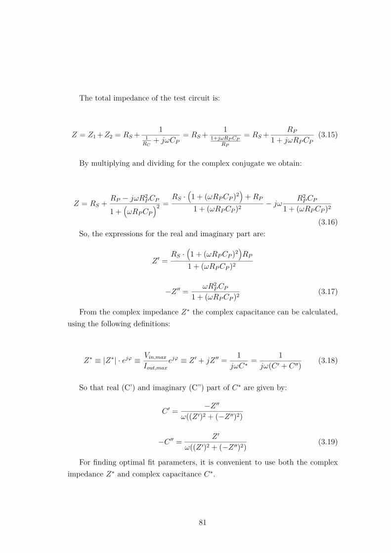
The total impedance of the test circuit is:

Z = Z1 +Z2 = RS + 11RC

+ jωCP= RS + 1

1+jωRPCPRP

= RS + RP

1 + jωRPCP(3.15)

By multiplying and dividing for the complex conjugate we obtain:

Z = RS + RP − jωR2PCP

1 +(ωRPCP

)2 =RS ·

(1 + (ωRPCP )2

)+RP

1 + (ωRPCP )2 − jω R2PCP

1 + (ωRPCP )2

(3.16)So, the expressions for the real and imaginary part are:

Z ′ =RS ·

(1 + (ωRPCP )2

)RP

1 + (ωRPCP )2

−Z ′′ = ωR2PCP

1 + (ωRPCP )2 (3.17)

From the complex impedance Z∗ the complex capacitance can be calculated,using the following definitions:

Z∗ ≡ |Z∗| · ejϕ ≡ Vin,maxIout,max

ejϕ ≡ Z ′ + jZ ′′ = 1jωC∗

= 1jω(C ′ + C ′′) (3.18)

So that real (C’) and imaginary (C”) part of C∗ are given by:

C ′ = −Z ′′

ω((Z ′)2 + (−Z ′′)2)

−C ′′ = Z ′

ω((Z ′)2 + (−Z ′′)2) (3.19)

For finding optimal fit parameters, it is convenient to use both the compleximpedance Z∗ and complex capacitance C∗.

81

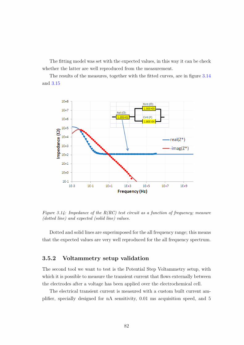
The fitting model was set with the expected values, in this way it can be checkwhether the latter are well reproduced from the measurement.

The results of the measures, together with the fitted curves, are in figure 3.14and 3.15

Figure 3.14: Impedance of the R(RC) test circuit as a function of frequency; measure(dotted line) and expected (solid line) values.

Dotted and solid lines are superimposed for the all frequency range; this meansthat the expected values are very well reproduced for the all frequency spectrum.

3.5.2 Voltammetry setup validation

The second tool we want to test is the Potential Step Voltammetry setup, withwhich it is possible to measure the transient current that flows externally betweenthe electrodes after a voltage has been applied over the electrochemical cell.

The electrical transient current is measured with a custom built current am-plifier, specially designed for nA sensitivity, 0.01 ms acquisition speed, and 5

82

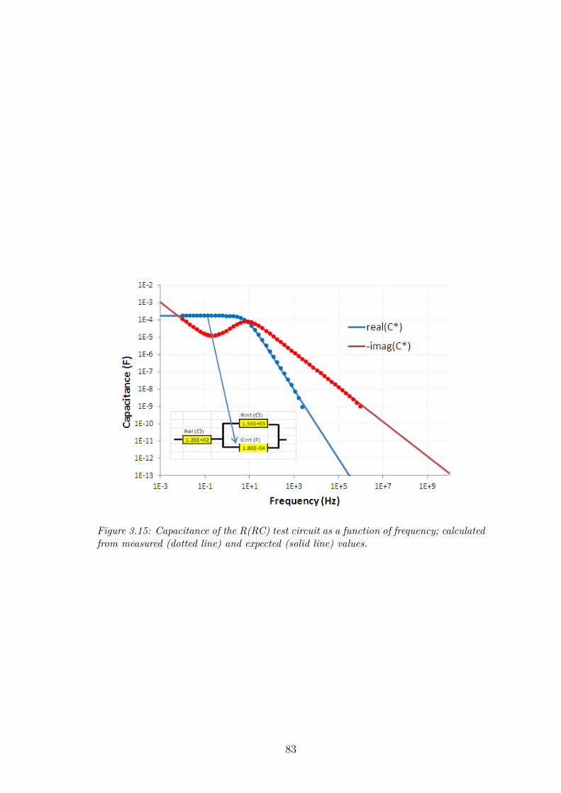
Figure 3.15: Capacitance of the R(RC) test circuit as a function of frequency; calculatedfrom measured (dotted line) and expected (solid line) values.

83

orders dynamic range (up to 100 microamperes).All transient current traces start from equilibrium (with zero voltage applied).

The initial capacitive charging currents (of mA during µs) are intentionally leftout of the traces. We applied to the test circuit a voltage step at 17 differentmagnitudes, from 0.01V up to 3V.

As shown before, the transient current can be expressed as

I = U

RS +RP

(1 + RP

RS

e−tRS+RP

RSRPC

)(3.20)

This transient current is not the exact analytical equation, because it assumedthat the electrical network contains ideal capacitance and resistance components,i.e. independent of frequency. The true capacitance and resistance componentsshow a slight frequency dependence. With involved mathematical analysis it canbe shown that in that case the factor in the transient current exponent will changevalue.

In the previous section we derived the expression for the impedance as afunction of frequency. The real and imaginary parts are given by

Z ′ =RS ·

(1 + (ωRPCP )2

)RP

1 + (ωRPCP )2

−Z ′′ = ωR2PCP

1 + (ωRPCP )2 (3.21)

In a typical transient current experiment, a voltage step is applied to thesystem. The formal expression is:

V (t) = Vt · u(t) with unit-step u(t) :=

0 if t < 0,

1 if t ≥ 0.

84

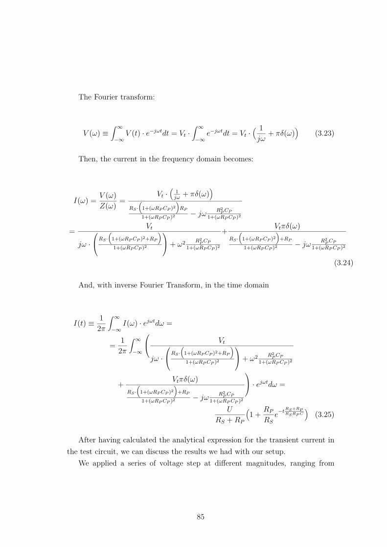
The Fourier transform:

V (ω) ≡∫ ∞−∞

V (t) · e−jωtdt = Vt ·∫ ∞−∞

e−jωtdt = Vt ·( 1jω

+ πδ(ω))

(3.23)

Then, the current in the frequency domain becomes:

I(ω) = V (ω)Z(ω) =

Vt ·(

1jω

+ πδ(ω))

RS ·(

1+(ωRPCP )2)RP

1+(ωRPCP )2 − jω R2PCP

1+(ωRPCP )2

= Vt

jω ·

RS ·(

1+(ωRPCP )2+RP)

1+(ωRPCP )2

+ ω2 R2PCP

1+(ωRPCP )2

+ Vtπδ(ω)RS ·(

1+(ωRPCP )2)

+RP1+(ωRPCP )2 − jω R2

PCP1+(ωRPCP )2

(3.24)

And, with inverse Fourier Transform, in the time domain

I(t) ≡ 12π

∫ ∞−∞

I(ω) · ejωtdω =

= 12π

∫ ∞−∞

Vt

jω ·

RS ·(

1+(ωRPCP )2+RP)

1+(ωRPCP )2

+ ω2 R2PCP

1+(ωRPCP )2

+ Vtπδ(ω)RS ·(

1+(ωRPCP )2)

+RP1+(ωRPCP )2 − jω R2

PCP1+(ωRPCP )2

· ejωtdω =

U

RS +RP

(1 + RP

RS

e−tRS+RP

RSRPC

)(3.25)

After having calculated the analytical expression for the transient current inthe test circuit, we can discuss the results we had with our setup.

We applied a series of voltage step at different magnitudes, ranging from

85

0.01V up to 3V, always by applying both positive and negative polarity to theelectrodes. By operating in this way it can be ensured that the test is symmetric,which is very important when dealing with true samples. Indeed, by first applyinga polarity and then the opposite one, it can be ensured that at the end of eachpotential step the charge distribution within the channel is as close as possibleto the homogeneous condition. In this way the symmetry of the samples is alsonot altered during time.

The following plots represent a comparison of the measurements with thefitted curve based on the expected values. For the charging phase we obtainedthe plot shown in figure 3.16.

Figure 3.16: I-t plot from the reference circuit used to validate the Voltammetry setup.

The black curve represent the transient current values obtained from the time

86

dependent solution for the R(RC) circuit:

I = U

RS +RP

(1 + RP

RS

e−tRS+RP

RSRPC

)(3.26)

Figure 3.16 represents the experimental results, and the fitting at 1 V. Tovalidate the setup, for each voltage, we compared the measured curve with acurve fitted using the RRC reference parameters.

All measured curves show a good agreement with the expected solution; nev-ertheless, for a time window ranging from 0.05s to 1s, all measured curves showa current decay which is not overlapped to the fitted curve (see figure 3.17).

Figure 3.17: Current normalized with applied voltage versus time. Reference circuitused to validate the Voltammetry setup.

As stated before, the time constant of the circuit is given by the product ofRS and C

87

τ = RS · C = 120 · 180× 10−6 = 0.216s

The measured curves, however, show a slower decrease on time.

3.5.3 Results of validation

For the EIS setup, the measured values have shown a perfect agreement with theexpected one. This achievement suggests us that the results obtained through theEIS setup can be used to study the charge transport processes occurring withinthe channel.

The Potential Step Voltammetry setup has been tested first by comparingthe measured results with the analytical expression for the transient current inthe time domain. The latter has been derived by applying the Fourier InverseTransform to the frequency dependent expression of the transient current. Thesecond check consisted in a graphical comparison of the measured and a fitted acurve, representing the approximated transient current flowing in the RRC circuitat a given voltage.

From this check, it turned out that there is a time window (from 0.05s to 1s)in which measured and fitted data are not in perfect agreement; while the fittedcurve decrease exponentially, with a time constant of 0.216s, the measured curvedecrease slowly (this imperfection could belong to the test circuit).

3.6 Set of Samples

The set of samples, which constitutes the core of this research project, has beenconceived such that the performance dependence on geometry and material canbe analyzed.There are also several parameters which have been experimentally varied for eachsample; these include ions concentration, influx rate, applied voltage and pH.Below is a table containing a list of all samples involved in the experimental in-vestigation. For each sample, as mentioned, the flow rate is calculated so as togenerate a velocity within the channel of 13.33 mm/s. Together with the speed,in the table, pressure values inside the channel are included; these have been

88

calculated with the Fourier series expansion described above ("Pressure sensor").The geometry of all samples is simple; they are all straight channels with rectan-gular cross section (in which the width is larger than the height). They can bedivided in two classes; a first group of samples, with electrodes in Carbon, BDDand Si, on the side walls of their channel. The fluid is entered within the channelfrom an inlet perpendicular to it. Then, once the solution has entered into thechannel and has interacted with the electric field generated by the electrodes,it is collected in three outlets. A narrow-section outlet in which the solution,when the applied signal is a voltage step, is rich in ions; then two, wide-section,central outlet (main outlet) carry most of the fluid towards the exit. The fluidthat passes through the main outlets has a very low ion content; in this sensethis class of devices is very close to the prototype that has to be realized. Figure3.18 shows both a topview and a cross-section schematic drawings of a Carbonsample; a first (3 mm thick, 5 cm wide) layer of PMMA is glued to the left andright Carbon electrodes (1 mm thick, separated by a width of 0.25 mm), and thebottom wall is obtained using a glue cover foil.For two materials (e.g. Carbon and BDD), we include also nice SEM (ScanningElectron Microscopy) images (figures 3.19, 3.20, 3.21), which will turn out to beuseful for the interpretation of some EIS data.Figure 3.22 shows an image of a carbon sample (ID: Jb30).

The second group (Figure 3.23, 3.24, and 3.25) includes channel samples withAu or Pt electrodes sputtered on two layers of glass (1 mm thick, 2 cm wide),which are then properly stacked and bonded as in figure 3.23 and 3.24. Usinga proper mask and etching technique, a multiple electrode configuration shapelike the one in figure 3.23 and 3.24 can be obtained. The lateral walls have beendesigned using SU-8. Their dimensions are smaller, but the main difference isrepresented by the number of electrodes. They have 5 electrode pairs, indepen-dent each other, which cover the top and the bottom walls of the channel; theseelectrode pairs are spaced from each other to make them electrically independent.In this way, by simply moving the electric connection to another electrode pair, itis possible to use the sample even if, for any reason, a given couple of electrodeshas been damaged. Figure 3.26 shows a photo of three gold devices belonging tothe second group of samples (ID: A1, A2, A3).

89

Figure 3.18: Cross-section (a) and top view (b) schematic drawings of a Carbon sample;a first (3 mm thick, 5 cm wide) layer of PMMA is glued to the left and right Carbonelectrodes (1 mm thick, separated by a width of 0.25 mm), and the bottom wall isobtained using a glue cover foil. a) View from the inlet (the central outlet is not visiblesince it is aligned with the inlet), a zoomed image of the gap is also shown (not inscale). b) View from top.

90

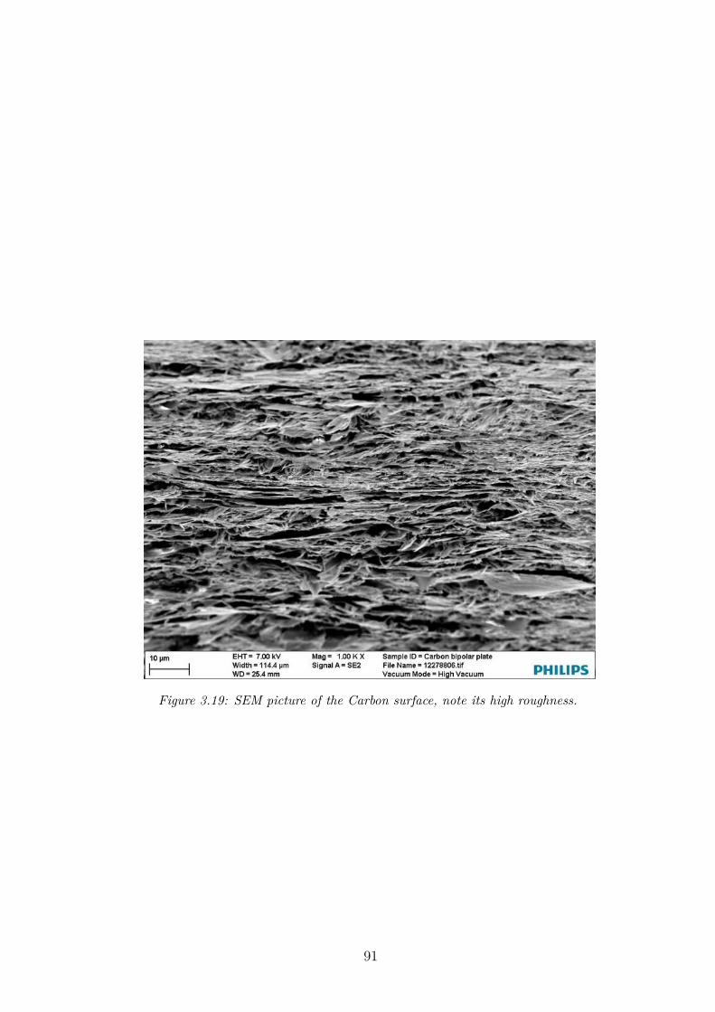
Figure 3.19: SEM picture of the Carbon surface, note its high roughness.

91

Figure 3.20: SEM picture of Carbon surface, increased magnifiaction; note the highsurface roughness.

92

Figure 3.21: SEM image of the BDD (Boron Doped Diamond) surface; note how, here,the surface roughness is much lower than in figure 3.19 and 3.20.

93

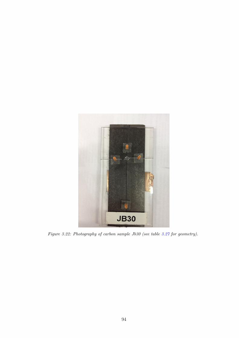
Figure 3.22: Photography of carbon sample Jb30 (see table 3.27 for geometry).

94

Figure 3.23: Cross-section (a) and top view (b) schematic drawings of a Pt sample; twostacked and bonded layers of glass (1 mm thick, 2 cm wide), with Pt (or Au) sputteredon top of them. After the etching, five independent electrode pairs are obtained. SU-8has been used to design the laterals walls. a) View from the inlet (the outlet is notvisible since it is aligned with the inlet). b) View from top.

Figure 3.24: Zoomed cross-section schematic drawing of a Pt sample; two stacked andbonded layers of glass (1 mm thick, 2 cm wide), with Pt (or Au) sputtered on top ofthem. After the etching, five independent electrode pairs are obtained. SU-8 has beenused to design the laterals walls. Not in scale.

95

Figure 3.25: Schematic representation of a sample belonging to the second class (Auand Pt). The axis perpendicular to the plane of the picture constitutes the width of thechannel.

Figure 3.26: Photography of three Au devices belonging to the second group of samples(see table 3.27 for geometry).

96

The first class of samples is very close to the real morphology and functionalityof the device that has to be realized. The structure of these samples has beendesigned to be used for separations experiments, which are not include in thepresent work, and constitute the next step of the research project.

The configuration of the second group of samples (having more than oneelectrode pair on the same device) is intended to be used for a parametric study.In this kind of study, a lot of measures have to be done, so the event of damageon one of the electrode pairs in not rare.

As it can be seen from the table, the gap between the electrodes ranges from5 µm and 250 µm, the width between 100 µm and 1mm , and the length is of3cm for the Au and Pt set of samples (not to be confused with the electrodelength, which is 5 mm), while for the set of samples with only one electrode pairthe length ranges from 55cm and 90cm. Together with the velocity within thechannel, also the time required to fill the channel, or the residence time for afluid particle, is reported in table 3.27. The last parameter is very useful whileflushing the system, since from its value one can have an idea of how many timesthe volume of the channel has been replaced.

3.7 Measuring Protocol

Through EIS we study how the impedance of the system varies in a very largedynamic range (from mHz up to MHz) by applying a voltage between the elec-trodes. Through Voltammetry tests, as described in the previous section, onecan measure the current flowing within the channel (transversal to the fluid flow)when a voltage step has been applied between the electrodes.

Different solutions (DI water, DI water with added HCl or KOH to reach apH from 4 up to 10 and DI water with added 3ppm, 30ppm, and 300ppm ofKCl) have been tested. For that reason a detailed procedure to be followed whenchanging type of solution has been developed and used to prepare each performedexperiment.

97

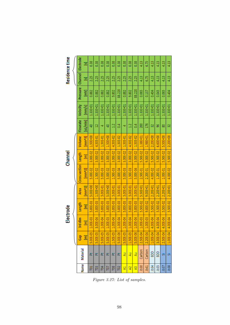
Figure 3.27: List of samples.

98

3.7.1 Changing working fluid

To quantitatively explain the results, so that the influence of various parameters(channel geometry, electrode material, fluid composition) on transport relatedphenomena is understood, it is crucial to ensure that the protocol used in theexperimental procedures takes into account and solves (or at least reduces) allpossible artifacts and problems.

In that sense, to be sure that the results are reliable, one has to introduce anumber of "checks" during the measuring procedure. The parameters that haveto be systematically controlled (because their values strongly affect the info weobtain) are the conductivity and the pH of the solution, the pressure within thechannel, the presence of parasitic EM effects, the presence of bubbles and air intothe channel.

To control and check all these parameters, we have built up an experimentalprotocol which, besides reducing all the artifacts, has been designed to ensurethat the measurements are as much reproducible and systematic as possible.

The operations involved in a test can be grouped in three phases:

1. Preparing the measurement

2. Measuring

3. Processing of the results

What follows is a list of all sequential steps involved in a typical experiment(cfr figure 3.29 for a better understanding of each step). These steps are here in-tentionally listed as a custom built up protocol; in this way each of the precautionused within the procedure is reported.

Preparation of measurement:

i. Flush DI water tap for at least 3 minutes (to be sure that the resistivityreaches at least a value of 1MΩ·cm).

99

ii. Fill a wash bottle with DI water (to wash and clean the pH and conductivitysensors). Alternatively fill a 600ml glass beaker with DI water.

iii. Fill a clean glass with 120ml of test solution (that amount of solution willbe used both for flushing the system and for the measure). If it’s a DI watertest, leave the glass in contact with atmosphere for '15 mins (in order tobe sure that the solution has reached equilibrium with the CO2 in the air).

iv. Prepare pH sensor for use: if the pH probe is in the storage solution,extract it and wash it under the DI water tap (or wash bottle); if it isjust dried and not in the storage solution, leave it for 1hour in the storagesolution to “activate” the sensor, and then rinse it under the DI water tap(or wash bottle).

v. Prepare conductivity sensor for use: it has to be left in contact withair, after having rinsed it with DI water. Before it can be used, it has to berinsed in the DI water tank.

vi. Fill a 60ml syringe with test solution, 30 ml of solution is used to flush thesystem at high flow rate (even by manually pushing the syringe) with thesample disconnected; then, after having connected the sample, use the last30ml to flush the system with the device connected (check that the pressuredoesn’t exceed 0.5 bar).

vii. After having flushed the system the syringe has to be disconnected. Whenthe syringe is disconnected, always block the soft Si tube (next tothe debubbler) with a crocodile clamp (see figure 3.28), so thatair cannot enter in the debubbler.

viii. Fill again a syringe with a volume of 6ml plus the amount of solution neededto run the test. Choose appropriate syringe size for the sample that hasto be tested (small cross-section samples require low flow rates, so a lowcross-section syringe has to be used). Note that, if the syringe volume usedfor the measurements is not 60 ml, the Diameter value has to be changedin the pump (check appendix 29 and 30).

100

ix. Fill two glasses (from now #1 and #2) with a small amount of solution('3ml) directly from the syringe.

x. Take note of the pressure value with no flow (and with sample and pumpdisconnected).

xi. Run the pump at high influx rate (so that the pressure reaches up to 12bar)

and fill a small glass (2.5ml) with the solution coming from the outlet. Notethat this step might not be applicable for the narrower samples due to thelow influx rate value, in these cases fill a glass with the solution coming fromthe outlet with the sample disconnected (to check if the system is clean).

xii. Measure the conductivity and temperature of the solution in glass #1 (filledwith the fluid directly from the syringe). All conductivity values arethen stored in a .xls template in KΩcm.

xiii. Measure the conductivity and temperature of the solution in the glass #3(filled with the fluid from the sample or otherwise with fluid from systemwithout sample).

xiv. Measure, after adding a small amount of NaCl (not needed for KCl so-lution), the pH of the solution in glass #2. Take note of value for thetemperature of solution, which can be read from the pH sensor display.

xv. Measure, after adding a small amount of NaCl (not needed for KCl so-lution), the pH of the solution in glass #3. Take note of value for thetemperature of solution, which can be read from the pH sensor display.

xvi. Set the influx rate at the standard value (specific for each sample, so thatthe velocity in the channel is 13.33mm/s), and take note of the pressurevalue (after it is stable).

xvii. For some samples it is necessary to block the side outlets to ensure thatnothing is sucked from the sample. In this case take note of the pressureafter having blocked the side outlets and take also note that the side outletshave been blocked.

101

xviii. Put the outlet tube into a clean glass (it can also be the same glass usedin steps xiii and xv to measure the outlet of the sample for the first time,thus from now it will be indicated as glass #3) which will be filled with thesolution coming through the sample.

xix. Electrically connect the sample.

xx. Close the Faraday Cover (always paying attention not to force the outletand inlet silicon tubes).

xxi. Take note of the Room Temperature value.

xxii. Calibrate the offset current, then close box, leave measurement running at0V for 30 minutes. If it drifts back, correct, and monitor for another 30minutes until it is stable (beware: electronics of transient current setupshows an offset current dependence on room temperature variation).

xxiii. If the measured pH, resistivity, and pressure are as expected, run the ex-periment. Take note of all values in an .xls file.

Measuring:

During the measurement, some tools that help to be sure that the conditionsof the system are close to the expected one are available. These tools includea pressure sensor (which is useful to check if the pressure is stable and is closeto the expected value), a scope (which shows both the EIS current and voltagewaves) and the software interface (which gives simultaneously an overview of thepoint acquired while measuring).

End of the experiment:

1. Check again the pressure and take note of the value.

2. Check again the Room Temperature and take note of the value.

102

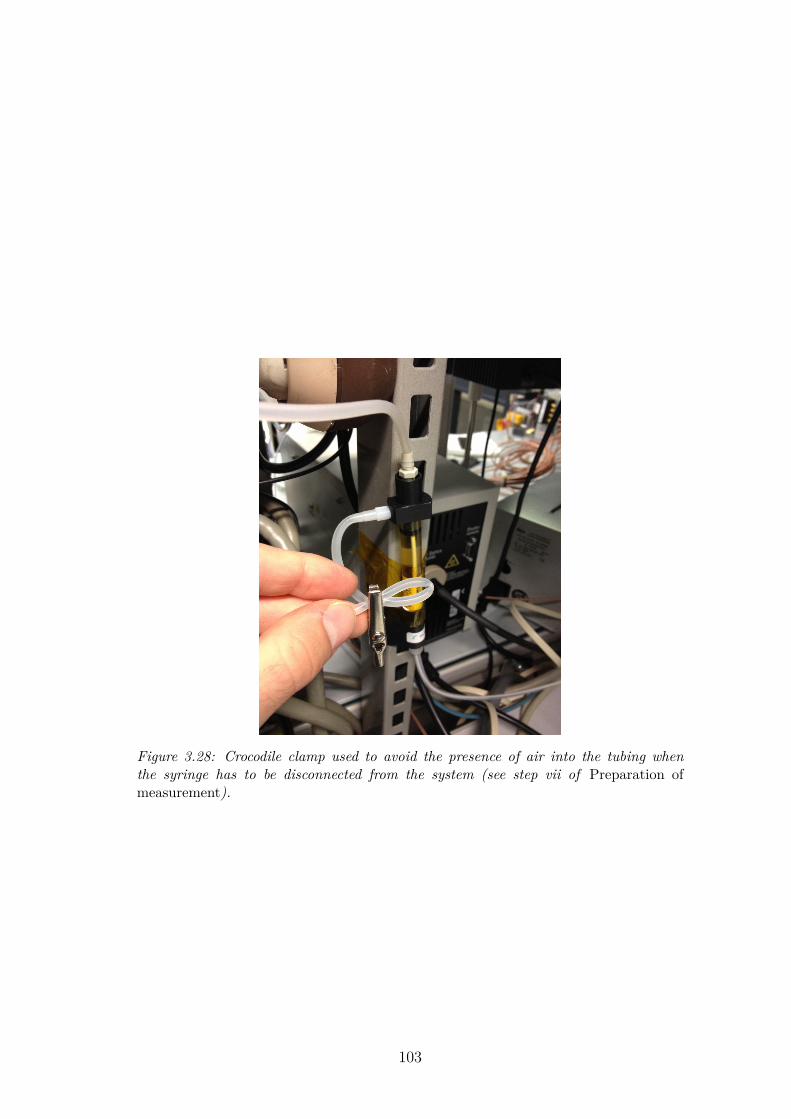
Figure 3.28: Crocodile clamp used to avoid the presence of air into the tubing whenthe syringe has to be disconnected from the system (see step vii of Preparation ofmeasurement).

103

3. Switch off the pump. Take note of the value for the pressure with no fluxbut with sample and pump connected.

4. Measure again the pH from glass #2 and the conductivity from glass #1.Take note of value for the temperature of solution, which can be read fromboth the pH sensor and conductivity display.

5. Measure the conductivity of the solution coming from the outlet (glass #3).

6. Measure the pH, after having added a small amount of NaCl (not needed forKCl solution), of the outlet solution. Take note of value for the temperatureof solution, which can be read from the pH sensor display.

7. Store the data in an excel sheet template including date of the measurement,sample ID, type of solution, AC rms voltage value, flow rate, all parameters(pH, conductivity, temperature of the solution, room temperature, pressure)checked before and after the measurement.

Post-processing of the results:

Two different templates (.xls files) for each measure have been developed.They constitute the core through which all measured data have been processed,and through which a physical interpretation of the response of the sample is given.

EIS data:

EIS experimental results have been stored and processed in a template orga-nized as in figure 3.29.

This template has been developed in order to obtain a tool through which themeasured data for Z∗(ω) can be converted into electrochemical parameters andother useful quantities.

As showed in the figure, the first step of the post-processing is represented bythe calculation of the complex capacity from the measured complex impedance.

104

Both complex impedance and complex capacitance are plotted as a function offrequency.

The template includes a space which has to be filled with the values from thesensors (pH, conductivity, pressure, and temperature). A table is organized suchthat both the values before and after the experiment are reported; this expedientprovides useful information when something weird is noticed within the results(such as higher impedance than expected).

Together with the measured values, as already previously described ("Theo-retical model based on RC network"), both Z∗(ω) and C∗(ω) from the equivalentelectrical network are plotted. The shape and the behavior of the fitted Z∗(ω)and C∗(ω) depends on several parameters, some of which are known.

The known quantities are the geometry parameters (length, width and height),pH and conductivity (since they are measured through the sensors before and afterthe measure), the electrical permittivity of the solution, and the mobility of theions.

One of the main aspects of the post-processing is represented by the compar-ison between expected and measured values. As already reported ("Theoreticalmodel based on RC network"), the geometrical capacitance is easily obtained bythe formula

Cgeom = ε0εrAdcell

(3.27)

The diffuse double layer capacitance, which depends on Cgeom, can be calcu-lated with the following relation

Cdl = ε0εrA

dcell

[ 12

√λ

tanh12

√λ− 1

]= Cgeom

[ 12

√λ

tanh12

√λ− 1

](3.28)

Also the ion resistance is a quantity which strongly affects the behavior ofZ∗(ω) and C∗(ω). Its expression is

Rion = dcell2neµA

(1 + 2.4

λ

( 12

√λ

tanh12

√λ− 1

))(3.29)

Summarizing, the steps involved in the post-processing analysis of an EIS

105

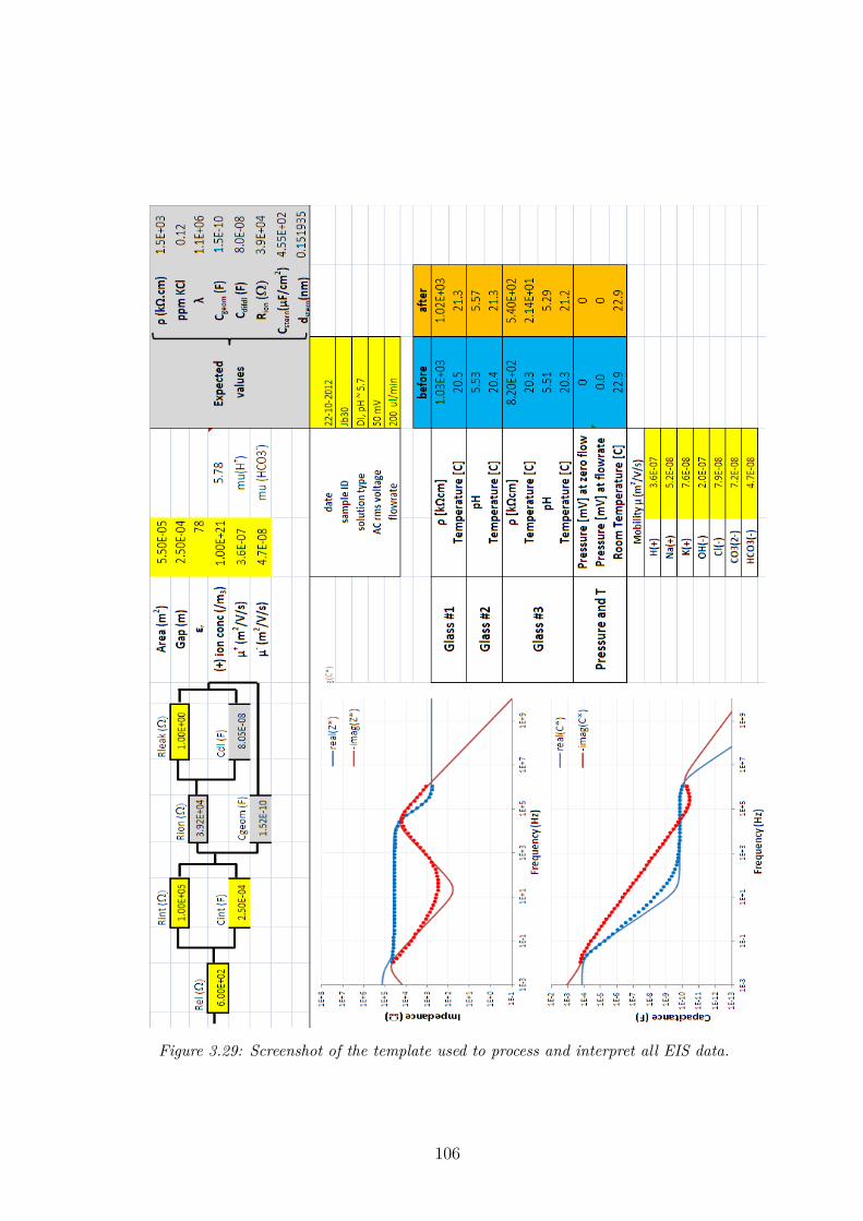
Figure 3.29: Screenshot of the template used to process and interpret all EIS data.

106

experiment are:

• Copy the impedance values as a function of frequency in the excel tem-plate. It automatically gives the values for the capacitance as a functionsof frequency, and plot both Z∗(ω) and C∗(ω).

• Fit the measurement with an R(RC(R[RC]C)) electrical network. Start byentering known values of dimensions, concentrations, mobilities (Cgeom, Cdl,Rion), then fit the values of other parameters (Rel, Rleak, Rint. Cint).

• Carefully have a look at the data, and try to give physical explanation towhat is plotted and to the values of the electrical network.

Transient current data

Also for transient current experiments a template has been developed. An-other reason that justifies the use of a template to process the measured results isthat, since the number of collected experiments is big, having all tests representedin the same way and with the same organization makes the interpretation andthe comparison of results easier.

The template for the Voltammetry tests is organized as follow. At the end ofan I-t test, the Labview software automatically creates a .txt file containing themeasured data. The content of this file is then copied in the template worksheet,which automatically plots both 0 −→ V and V −→ 0 phases in a double logarithmicgraph. A cell with a ×100 amplification factor restores the current values to theiroriginal values.

Both for 0 −→ V and V −→ 0 graph, the template offers the possibility toadjust the current offset, its value can be read from the last current value of thedischarging phase plot.

The last acquired current value for the charging phase, for each voltage, isplotted as a function of V; in this way an I-V plot with the steady state valuesis obtained. The latter is very useful in interpreting and analyzing electrolysisfeatures and ranges.

107

Also this template is equipped with a table which has to be filled with all themeasurements from the sensors (conductivity, pH, pressure, and Temperature).

3.7.2 Order of measurements

All tests have been performed following the procedure described in the previoussection. Another protocol, which makes the experimental analysis more system-atic, has been designed; it describes the order with which each measurement,on a given sample, has been done. This protocol has been applied to all testedsamples.

The order of measurements has been designed so as to reduce the effect ofall artifacts and alterations. The main issue that has to be overcome is thealteration of the test solution properties (resistivity, ion concentration and pH)due to impurities. The most sensitive fluid, in this sense, is DI water. Due tothe very low charged species content, indeed, DI water is very sensitive to anyvariation in ions concentration; it is therefore appropriate to use it for the veryfirst characterization of a sample. Also, starting with DI water, allows to comparethe results of a given sample in its “virgin state” to a second DI water test, onthe same sample, done after all KCl experiments; this comparison helps to checkwhether the response of the device shows significant differences after a completerun of the protocol.

For the above mentioned reasons, the first fluid we introduced into the channelis DI water. After having characterized a sample using DI water, the followingstep of the procedure is a series of tests with a solution containing a graduallyincreasing amount of KCl. The first series of tests with a solution of 3ppm KCldissolved in DI water, then 30ppm, and finally 300ppm.

As previously mentioned, a last test, again with DI water, is conducted toensure that the result of the first DI water measure is reproduced, and also tostore the tested sample in a "clean environment", with the lowest possible amountof charged species.

For each type of solution the tested sample is first characterized through EIS(with and without flow), and then a sequence of transient current measures isconducted. Through the Voltammetry test, two main goals have been achieved:

108

the first is the characterization of the material which shows electrolysis at thehighest voltage, the second being the study of flow effects on the steady statecurrent.

To reach the first goal, a series of Voltammetry experiments at different volt-age, for different material, has been developed.

To study the influence of the flow rate on the steady state current, for eachsolution, a sequence of tests at 2V has been developed, which can be summarizedas follows

• Complete series of step voltages (17 different amplitudes; i.e. from 0.01 Vup to 2.2 V) at 13.33mm/s

• 2V at 13.33 mm/s

• 2V without flow

• 2V at 13.33 mm/s

• (Optional) Complete series of step voltages (17 different amplitudes) at13.33mm/s (to see if the first test is reproduced)

The result of this sequence of tests has been compared with simulations. Indeed,as described previously, measurements only constitute half of the tools throughwhich we have drawn conclusions and figured out a physical picture of what hap-pens when a voltage step of given amplitude is applied to sample. The secondtool is represented by a finite element simulation (COMSOL), which provides anumerical integration of all differential equation describing the physics involvedin a transient test. The results of these two tools are then compared, trying toachieve an agreement between them. Since a systematic experimental procedure,with several checks, has been developed, the experimental results can be con-sidered reliable. So, every gap between measurements and simulations has beenfilled by adjusting the latter in order to fit the experimental framework. Thesequence of I-t tests above listed has been developed in order to offer a referencefor the simulations. The entire protocol has been repeated for each solution.

In accordance with the procedure we developed, a complete sequence of mea-sure, for a given sample, can be summarized as follows

109

• DI water

1. With flow: EIS

2. With flow: I-t 0-3V (2x 0V duration)

3. With flow: 2V (repeat 2x)

4. Without flow: 2V (2x 0V, repeat 2x)

5. With flow: 2V (2x 0V, repeat 2x)

6. With flow (Optional) : Trans 0-3V (to see if the first result is repro-duced)

• Change fluid: 3ppm KCl

1. With flow: EIS

2. With flow: I-t 0-3V (2x 0V duration)

3. With flow: 2V (repeat 2x)

4. Without flow: 2V (2x 0V, repeat 2x)

5. With flow: 2V (2x 0V, repeat 2x)

6. With flow (Optional) : Trans 0-3V (to see if the first result is repro-duced)

• Change fluid: 30ppm KCl

1. With flow: EIS

2. With flow: I-t 0-3V (2x 0V duration)

3. With flow: 2V (repeat 2x)

4. Without flow: 2V (2x 0V, repeat 2x)

5. With flow: 2V (2x 0V, repeat 2x)

6. With flow (Optional) : Trans 0-3V (to see if the first result is repro-duced)

• Change fluid: 300ppm KCl

110

1. With flow: EIS

2. With flow: I-t 0-3V (2x 0V duration)

3. With flow: 2V (repeat 2x)

4. Without flow: 2V (2x 0V, repeat 2x)

5. With flow: 2V (2x 0V, repeat 2x)

6. With flow (Optional) : Trans 0-3V (to see if the first result is repro-duced)

• DI water (repeat to see if sample degraded by exposure to high KCl, andsafely store after measurement series)

1. With flow: EIS

2. With flow: Trans 0-3V (2x 0V duration. check for asymmetry, if somove to next electrode pair. Beware of T-changes)

3. With flow: 2V (repeat 2x)

4. Without flow: 2V (5x 0V, repeat 2x)

5. With flow: 2V (5x 0V, repeat 2x)

6. With flow (Optional) : Trans 0-3V (to see if the first result is repro-duced)

Note that, only for a first set of EIS tests on some samples, we have alsotried to reduce the influx rate. The EIS results, also in this case, showed that nosignificant variation in Cint can be seen by comparing the test with standard andreduced flow rate.

The measures with KCl solutions have been performed by reproducing thesame fluid dynamic conditions used for DI water: the influx rate, for each sample,has been calibrated such that a velocity of 13.33mm/s was generated within thechannel.

111

Chapter 4

Experimental results

4.1 EIS measurements on channel samples

4.1.1 Jb30 (Carbon sample) EIS results

After having described the setup, the protocol, and the model used to fit themeasured data, the experimental results can be showed and discussed.A typical series of EIS measurements is shown here, done on a carbon sample (ID:Jb30, see table 4.1 for dimensions). Together with deionized water, equilibratedwith CO2 in the air (i.e. pH =5.7), we prepared three solutions with differentconcentrations of KCl (see 4.2).From concentrations, knowing the mobilities of charged species (see table 4.3),one can easily calculate the resistivity (in kΩ· cm) of the solution as follows

ρexp = 1(n · (∑i µi) · e

)· 10

(4.1)

Where µi is the mobility of charged species i, and e is the electric charge (i.e.1.6×10−19 C). With n we indicated the concentration of ions in m−3, which isrelated to the concentrations in ppm nppm by the following expression

112

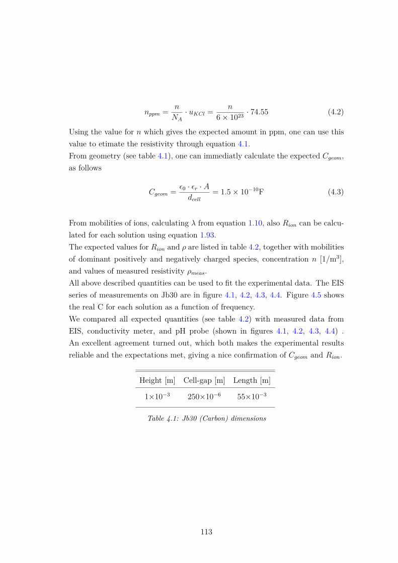
nppm = n

NA

· uKCl = n

6× 1023 · 74.55 (4.2)

Using the value for n which gives the expected amount in ppm, one can use thisvalue to etimate the resistivity through equation 4.1.From geometry (see table 4.1), one can immediatly calculate the expected Cgeom,as follows

Cgeom = ε0 · εr · Adcell

= 1.5× 10−10F (4.3)

From mobilities of ions, calculating λ from equation 1.10, also Rion can be calcu-lated for each solution using equation 1.93.The expected values for Rion and ρ are listed in table 4.2, together with mobilitiesof dominant positively and negatively charged species, concentration n [1/m3],and values of measured resistivity ρmeas.All above described quantities can be used to fit the experimental data. The EISseries of measurements on Jb30 are in figure 4.1, 4.2, 4.3, 4.4. Figure 4.5 showsthe real C for each solution as a function of frequency.We compared all expected quantities (see table 4.2) with measured data fromEIS, conductivity meter, and pH probe (shown in figures 4.1, 4.2, 4.3, 4.4) .An excellent agreement turned out, which both makes the experimental resultsreliable and the expectations met, giving a nice confirmation of Cgeom and Rion.

Height [m] Cell-gap [m] Length [m]

1×10−3 250×10−6 55×10−3

Table 4.1: Jb30 (Carbon) dimensions

113

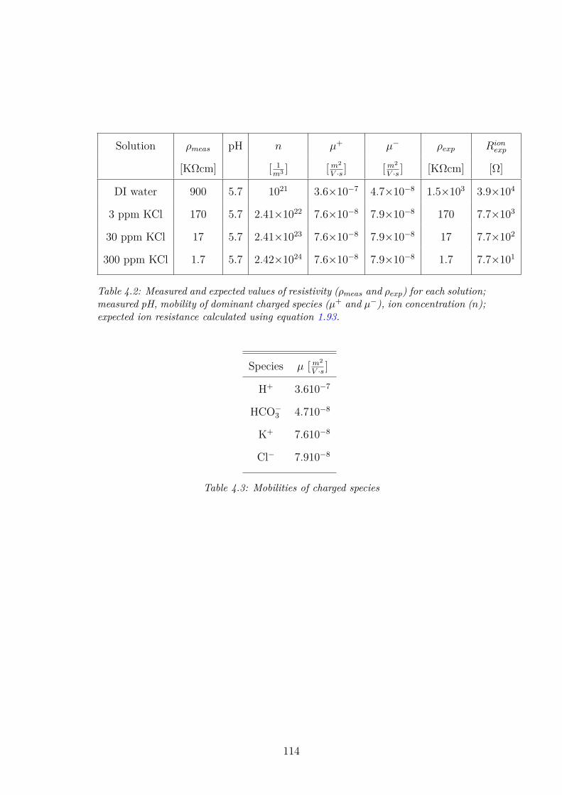
Solution ρmeas pH n µ+ µ− ρexp Rionexp

[KΩcm] [ 1m3 ] [m2

V ·s ] [m2

V ·s ] [KΩcm] [Ω]

DI water 900 5.7 1021 3.6×10−7 4.7×10−8 1.5×103 3.9×104

3 ppm KCl 170 5.7 2.41×1022 7.6×10−8 7.9×10−8 170 7.7×103

30 ppm KCl 17 5.7 2.41×1023 7.6×10−8 7.9×10−8 17 7.7×102

300 ppm KCl 1.7 5.7 2.42×1024 7.6×10−8 7.9×10−8 1.7 7.7×101

Table 4.2: Measured and expected values of resistivity (ρmeas and ρexp) for each solution;measured pH, mobility of dominant charged species (µ+ and µ−), ion concentration (n);expected ion resistance calculated using equation 1.93.

Species µ [m2

V ·s ]

H+ 3.610−7

HCO−3 4.710−8

K+ 7.610−8

Cl− 7.910−8

Table 4.3: Mobilities of charged species

114

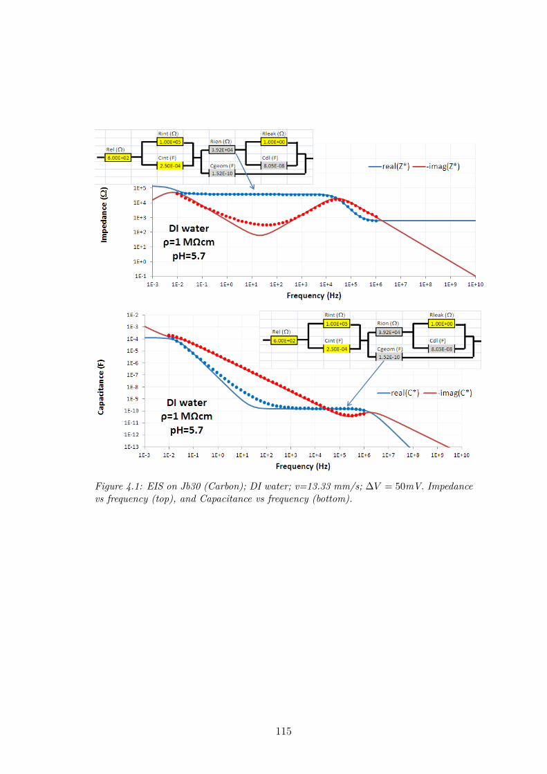
Figure 4.1: EIS on Jb30 (Carbon); DI water; v=13.33 mm/s; ∆V = 50mV. Impedancevs frequency (top), and Capacitance vs frequency (bottom).

115

Figure 4.2: EIS on Jb30 (Carbon); 3 ppm KCl; v=13.33 mm/s; ∆V = 50mV.Impedance vs frequency (top), and Capacitance vs frequency (bottom).

116

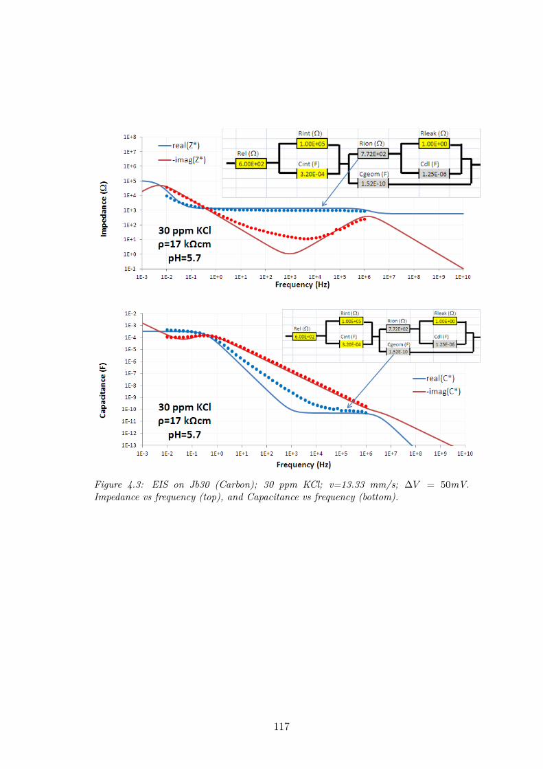
Figure 4.3: EIS on Jb30 (Carbon); 30 ppm KCl; v=13.33 mm/s; ∆V = 50mV.Impedance vs frequency (top), and Capacitance vs frequency (bottom).

117

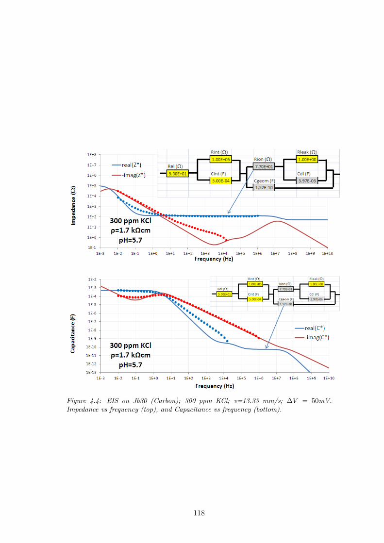
Figure 4.4: EIS on Jb30 (Carbon); 300 ppm KCl; v=13.33 mm/s; ∆V = 50mV.Impedance vs frequency (top), and Capacitance vs frequency (bottom).

118

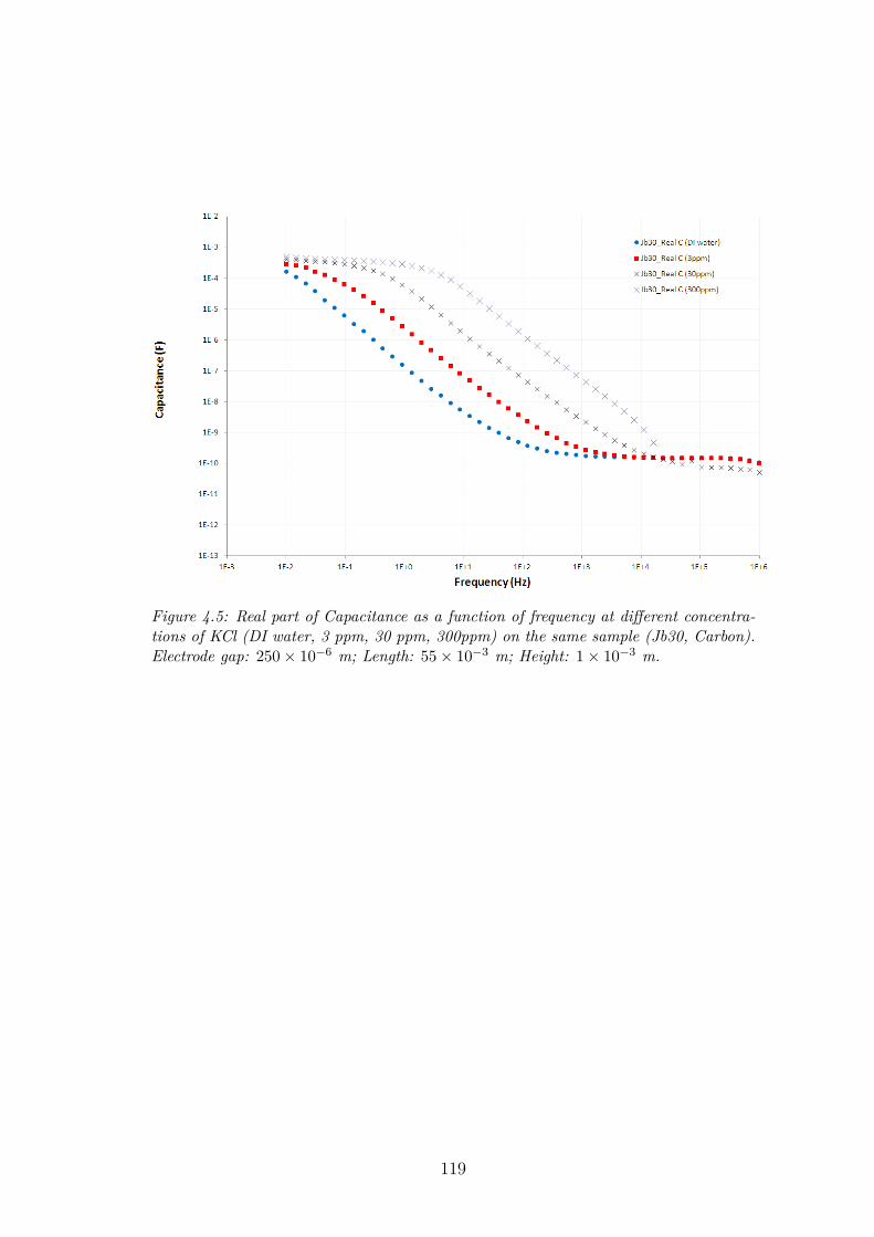
Figure 4.5: Real part of Capacitance as a function of frequency at different concentra-tions of KCl (DI water, 3 ppm, 30 ppm, 300ppm) on the same sample (Jb30, Carbon).Electrode gap: 250× 10−6 m; Length: 55× 10−3 m; Height: 1× 10−3 m.

119

4.1.2 Validate dimensions of sample channels

Based on the electrical network model, the electrophoretic mobilities and concen-trations of the solution can be calculated and verified. Also, by using the formulafor the capacitance of a parallel-plate capacitor

C = ε0εrA

dcell(4.4)

the consistency of the cell gap d can be validated.For all samples this comparison showed a good agreement between the valueextracted from measured C and the expected nominal gap.This achievement is also very useful in the analysis of samples degradation duringtime. Indeed, if electrode layers break loose for any reason, thus increasing thecell gap, this can be easily checked and verified with EIS.

4.1.3 Low frequency Stern capacitance observed, inde-

pendent of concentration and pH

As previously described ("Theoretical model based on RC network") a low fre-quency capacitive behavior appears in all EIS results. We probed the dependenceof this parameter on several quantities.

• Dependence on flowrate

The first check has been to reduce (and even set to zero) the flow rate, to seeif this quantity was correlated to an accumulation process of charges next tothe electrode interfaces due to the flux. By comparing EIS results of tests withand without flow, no significant difference between the two values was found (seeappendix A, figure 28).

• Dependence on electrode material & KCl concentration

The very high value for the capacitance suggests that the charge has to be con-densed in a very thin space at electrodes interface; for this reason we named it

120

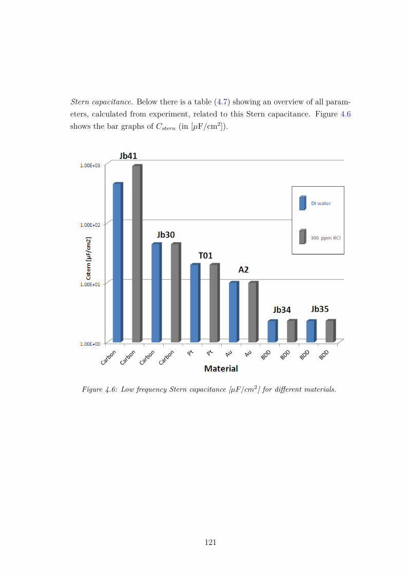
Stern capacitance. Below there is a table (4.7) showing an overview of all param-eters, calculated from experiment, related to this Stern capacitance. Figure 4.6shows the bar graphs of Cstern (in [µF/cm2]).

Figure 4.6: Low frequency Stern capacitance [µF/cm2] for different materials.

121

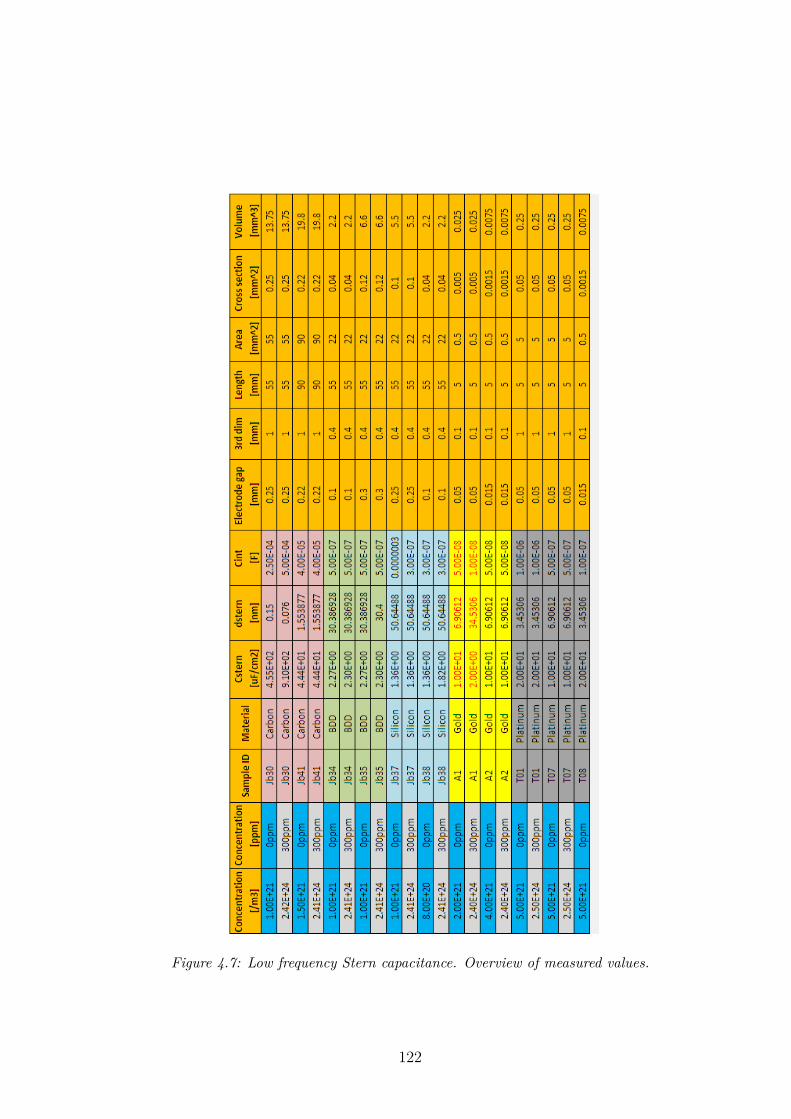
Figure 4.7: Low frequency Stern capacitance. Overview of measured values.

122

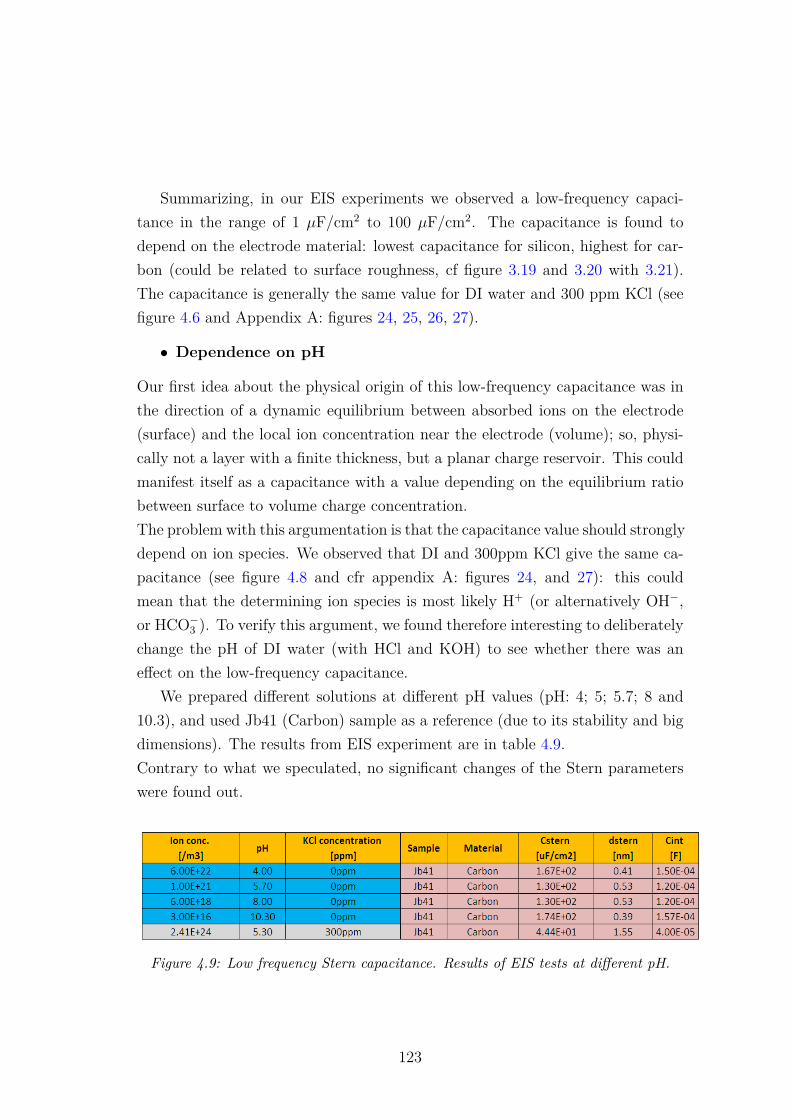
Summarizing, in our EIS experiments we observed a low-frequency capaci-tance in the range of 1 µF/cm2 to 100 µF/cm2. The capacitance is found todepend on the electrode material: lowest capacitance for silicon, highest for car-bon (could be related to surface roughness, cf figure 3.19 and 3.20 with 3.21).The capacitance is generally the same value for DI water and 300 ppm KCl (seefigure 4.6 and Appendix A: figures 24, 25, 26, 27).

• Dependence on pH

Our first idea about the physical origin of this low-frequency capacitance was inthe direction of a dynamic equilibrium between absorbed ions on the electrode(surface) and the local ion concentration near the electrode (volume); so, physi-cally not a layer with a finite thickness, but a planar charge reservoir. This couldmanifest itself as a capacitance with a value depending on the equilibrium ratiobetween surface to volume charge concentration.The problem with this argumentation is that the capacitance value should stronglydepend on ion species. We observed that DI and 300ppm KCl give the same ca-pacitance (see figure 4.8 and cfr appendix A: figures 24, and 27): this couldmean that the determining ion species is most likely H+ (or alternatively OH−,or HCO−3 ). To verify this argument, we found therefore interesting to deliberatelychange the pH of DI water (with HCl and KOH) to see whether there was aneffect on the low-frequency capacitance.

We prepared different solutions at different pH values (pH: 4; 5; 5.7; 8 and10.3), and used Jb41 (Carbon) sample as a reference (due to its stability and bigdimensions). The results from EIS experiment are in table 4.9.Contrary to what we speculated, no significant changes of the Stern parameterswere found out.

Figure 4.9: Low frequency Stern capacitance. Results of EIS tests at different pH.

123

Figure 4.8: Real part of Capacitance as a function of frequency at different concentra-tions (DI water, 30 ppm, 300ppm) on the same sample (T01, Pt).

• Summary of low frequency capacitance results

Summarizing we can conclude that the low frequency capacitance is independenton pH, ion concentration and influx rate. The only parameter that affects thevalue of the Stern capacitance is the electrode material. To obtain some insights itcould be interesting to investigate and study the interaction mechanism betweencharged species and different materials in a solid/liquid interface (Adsorption).However, we must point out that, given the low applied voltage used in EIS,the conclusions made on the capacitive behavior at low frequencies are only validunder the assumption of a small voltage (of the orders of mV). At higher voltages,in fact, migration becomes more important, while the diffusion can be neglected,then, as the electrokinetic regime changes radically, it is not possible to extendthe above findings implicitly also for higher voltages.

124

4.2 Validate dimensions of channel samples by

pressure drop

To validate the dimensions of a given channel, not only the EIS apparatus canbe used. As reported previously (see "Pressure sensor"), it is possible to makea comparison between the expected value for the pressure within the channeland the measured value. Once the sensor has been calibrated and its output isconsidered reliable, it is possible to check whether the dimensions of the channelare or not in agreement with the expected value.This comparison proved very useful during the tests on small samples (15 µmand 5 µm electrodes gap), since it helped us in finding some leakages within thesystem. A first leakage was found upstream of the debubbler, and eliminated;after this correction the samples with a gap of 15 µm showed a pressure value inagreement with the expected value, while for the sample with a gap of 5µm theagreement was not so good.To overcome this issue, some new (gas tight) syringes have been ordered andtested, but they didn’t solve the problem. A more tight tubing connectors mayprove useful in solving this issue.An alternative solution is using a flow sensor to adjust the pressure until thedesired value is reached.

4.3 Transient measurement on channel samples

Through Voltammetry we studied the I(t) response of all samples. As previouslydescribed (Potential step Voltammetry"), in a typical I-t test, a number of differentvoltage step amplitudes are applied to the sample, in both polarities. A zerovoltage step (discharging phase) of 200 s is interposed between every voltageswitch (and change).From the shape of the curve obtained from a measurement, it is possible to analyzetransport related dynamics, to see which mechanism is limiting the transport ofcharged species, to estimate the voltage at which electrolysis occurs for a given

125

material, and to both see and understand the effects of geometry or flow ratechanges on transport.A systematic characterization has been conducted over the set of samples. Theprocedure described in the last chapter, together with the checks of all importantquantities, has been followed to obtain reliable results.

4.3.1 Dependence of electrode material on steady I-V curves

(electrolysis)

To identify the material that shows electrolysis at the highest applied voltage, sev-eral samples with different electrode material have been tested using 300ppm ofKCl dissolved in water. As described in chapter 2 (section Potential step Voltam-metry"), an I-V plot can be created by taking, for each voltage, the steady statecurrent value (last acquired data from the I-t curve). The electrolysis mechanismis voltage activated; furthermore, different materials have different threshold volt-age at which electrolysis process starts. In the first chapter we showed how theefficiency of separation mechanism increases if the applied voltage increase. But,at the same time, if the applied voltage exceeds the electrolysis threshold, thecurrent increases due to reactions occuring at electrodes surface. In this regime,new products are generated, thus compromising the performance of the device.To enhance the performance of our devices, a key aspect is represented by theresearch of the material which shows the highest threshold voltage.To achieve this result, different devices have been tested by deliberately exag-gerating the higher applied voltage amplitudes of the series. For each material,different attempts have been tried, to find the range at which the electrolysisthreshold was reached and exceeded.The tested materials have been carefully chosen after a detailed literature re-search. We expected BDD to be the best performing material, followed by Car-bon, Au and Pt; Si, even if included in the plot, being a semiconductor, has notbeen included in this comparison.Because of differences in the geometry of the samples we compared, current den-sity (A/mm2) has been used for the comparison instead of the current. In this

126

way differences in electrode area have been eliminated, and material is almostthe only factor influencing differences in resulting curves. To totally remove fromthis comparison any kind of parameter different from the electrode material, thecurrent density has to be multiplied for the cell gap (which also differs from onesample to another), thus obtaining a quantity that we named "bulk currentdensity", with dimensions of A/mm.The result is summarized in Figure 4.10 (current density) and 4.11 (bulk currentdensity).

As can be seen in figure 4.10, the experimental results are in nice agreementwith the expected results [13], [14] for both the BDD sample, which shows elec-trolysis at the highest threshold voltage ('4V), and Pt sample, which has thelowest value ('2.2V). The Carbon and Au, differently from what expected, showsa comparable threshold voltage ('3V).From figure 4.11 an interesting trend shows up: for all materials the plateau isat the same bulk current density value (2.5·10−7 A/mm), so the current level ismaterial independent (the only effect of material is shifting the voltage amplitudeat which it shows up). Furthermore, by comparing figure 4.10 with figure 4.11,one can see that, in the plateau region, the current density is different for sampleswith different cell gap. This result could be an indication that migration is limit-ing the dynamic (different electric field for different electrode gap). Nevertheless,in this regime (different for each material), an increase in applied voltage doesn’tchange the measured bulk current density. As it will be shown in the next section,a detailed analysis of the diffusion time could give an explanation to this strangeresult.

4.3.2 Characterization of transient current

A second study has been conducted by means of Potential step Voltammetry. Weperformed a parametric analysis of the effects of several parameters on transientcurrent.The main quantities that have been varied are the flow rate, applied voltage,and type of solution. To analyze the effect of flow rate on the measured currentwe choose Pt as a reference material, mainly due to its lower threshold voltage,

127

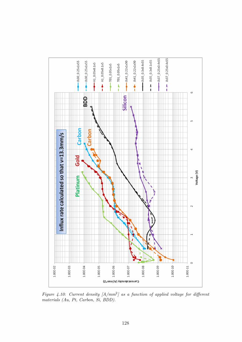
Figure 4.10: Current density [A/mm2] as a function of applied voltage for differentmaterials (Au, Pt, Carbon, Si, BDD).

128

Figure 4.11: Bulk Current density [A/mm] as a function of applied voltage for differentmaterials (Au, Pt, Carbon, Si, BDD).

129

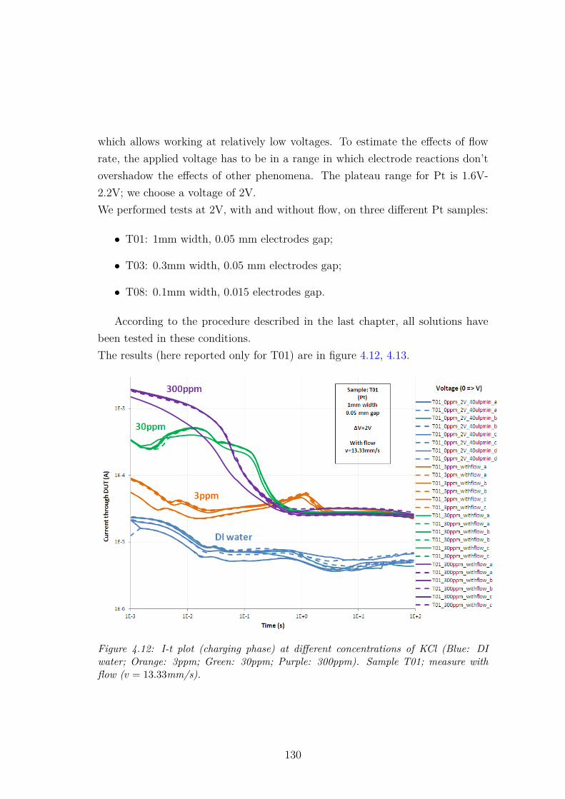
which allows working at relatively low voltages. To estimate the effects of flowrate, the applied voltage has to be in a range in which electrode reactions don’tovershadow the effects of other phenomena. The plateau range for Pt is 1.6V-2.2V; we choose a voltage of 2V.We performed tests at 2V, with and without flow, on three different Pt samples:

• T01: 1mm width, 0.05 mm electrodes gap;

• T03: 0.3mm width, 0.05 mm electrodes gap;

• T08: 0.1mm width, 0.015 electrodes gap.

According to the procedure described in the last chapter, all solutions havebeen tested in these conditions.The results (here reported only for T01) are in figure 4.12, 4.13.

Figure 4.12: I-t plot (charging phase) at different concentrations of KCl (Blue: DIwater; Orange: 3ppm; Green: 30ppm; Purple: 300ppm). Sample T01; measure withflow (v = 13.33mm/s).

130

Figure 4.13: I-t plot (charging phase) at different concentrations of KCl (Blue: DIwater; Orange: 3ppm; Green: 30ppm; Purple: 300ppm). Sample T01; measure withoutflow (v = 0mm/s).

131

By comparing the current for different KCl solutions in the plateau region,we noticed that the dependence of current on ions concentration disappears inthe steady state, meaning that the measured current is not generated by the K+

and Cl− ions. Indeed, in the transient region, different concentrations give riseto different currents (I is higher as concentration increases), but, at the steadystate, all curves settle down to the same value (screening region). In this regionthe only contribution to current is due to water autoionization and reactions atthe electrodes.DI water shows a higher steady state current in the measures without flow thanin the experiments with flow. This result could be considered strange; anyway, anexplanation can be found. In a DI water test without flow, once H+ and OH− havebeen separated, autoionization acts generating new H+ and OH− ions, which alsoare carried by the electric field (since DI water doesn’t generate screening) towardsthe sides; this process, in which autoionization creates ions and applied voltageseparates them, contributes to the measured current. When flow is present, afterthe first separation of H+ and OH−, the volume in the center of the channelis replaced with a new amount of solution in which H+ and OH− are alreadyequilibrate, so the effect of autoionization on measured current is less evidentthan without flow, and the global result is a lower steady state current.

4.3.3 I-V on different geometries

An interesting picture turns out when the I-V plot of samples with differentgeometry is compared (Figure 4.14).

By analysing the I-V curves, it can be noted that the smaller the electrodesgap, the higher is the plateau current density. It has been already shown that thesteady-state current, in the plateau region, is independent on voltage, thus mean-ing that the migration is not contributing to measured current. Indeed, diffusionof H+, OH−, H2, and O2 is the process that drives and control the dynamicin this regime. H+, formed at positive electrode, diffuse due to a concentrationgradient towards the center of the channel; the same process, occurring in theopposite direction, drives the OH− from negatively charged electrode towardsthe center of the channel. In the center, H+ and OH− recombine, thus giving

132

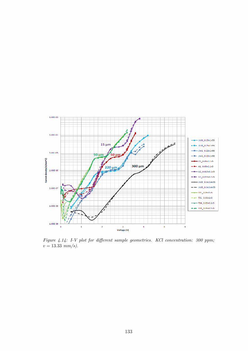
Figure 4.14: I-V plot for different sample geometries. KCl concentration: 300 ppm;v = 13.33 mm/s).

133

current. The limiting rate is the diffusion of species from the sides of the channelto the center.The I-V curves showed in picture 4.14, clearly show what described until now.Indeed, in the plateau region, the current is independent on applied voltage (nomigration), and a lower gap gives an higher current density (more ions per secondreach a unit element of electrode surface).The diffusion time is given by

tdiff 'd2cell

2D = d2cell

2µkTe

= d2cell

2µ · 25mV (4.5)

while the migration time is

tmig = dcellµ · E

= dcell · dfieldµ ·∆V (4.6)

So, if the field is reduced of a factor of 102, due to a decrease of the thickness(dfield) through which it is condensed, diffusion becomes relevant. Figure 4.16shows that the electric field is reduced by 100, thus making this speculation evenmore reliable.

4.4 Comparison with simulations

To deeply understand the physical picture involved in our experiment, the ulti-mate proof is represented by the comparison of experimental results with simula-tions. Figure 4.15 shows a comparison of experimental results from measurementson T01 (Pt sample) with an applied voltage of 2 V, and different concentrationsof KCl (0, 3, 30 , 300 ppm). Each condition of applied voltage and ion concen-tration has been implemented in the model (electrode material is not included inthe model).

From figure 4.15 it is clear that a qualitative agreement between simulations

134

Figure 4.15: I-t plot from simulations (left graph) and experiments (right plot). Differ-ent concentrations of KCl (0, 3, 30, 300 ppm); v = 13.33 mm/s); ∆V = 2 V.

135

and experiments has been obtained. The transient shape of all curves is domi-nated by migration of ions, thus giving a higer current at higher concentrationsof KCl. After a certain time, which is inversely proportional to the concentrationof ions, the accumulation of K+ and Cl− at the opposite charged electrodes (seefigure 4.18) is such that the electric field in the bulk is screened, and migrationbecomes negligible (all curves stabilize at the same current).The last speculation can be verified with simulation. In figure 4.16 the timedependence of the normalized electric field in different regions of the channel isplotted. We indicated with 1 and 9, respectively, the left (positively charged)and right (negatively charged) walls of the channel, with 3 and 7 the limit of thediffuse double layers, and with 5 the center of the channel. It is evident that,between 10−4 s and 10−3 s, the electric field becomes negligible everywhere, beingall condensed at the sides of the channel.

In the steady-state the measured current results from H+ and OH− injectionat the electrodes and recombination in the bulk. This picture becomes evident insimulations results. Figure 4.17 shows the contribution to current of each speciesas a function of time (for a solution of 300 ppm of KCl at 2V). It is evident thatin the transient region (from initial time until 10−4 − 10−3 s) the external cur-rent is determined by K+ and Cl−, while, at longer time, H+ and OH− becomedominant due to their rise in concentration.

Another hypothesis that can be verified with simulations is the mechanismof transport that carries the H+ and OH− created due to injection towards thecenter of the channel. Figure 4.19 shows the steady-state distribution, within thecell gap, of the concentrations of all charged species. By analysing the concen-tration profile of H+ and OH− it is clear that diffusion acts carrying them fromtheir generation point towards the center of the channel, where they recombine,thus giving rise to an external current.

Also the recombination of H+ and OH− can be studied with the model. Whatfollows (figure 4.20) is a plot, at different times, of the [H+][OH−]

Kwratio as a func-

tion of the normalized coordinate of the cell gap. It can be easily noted that the

136

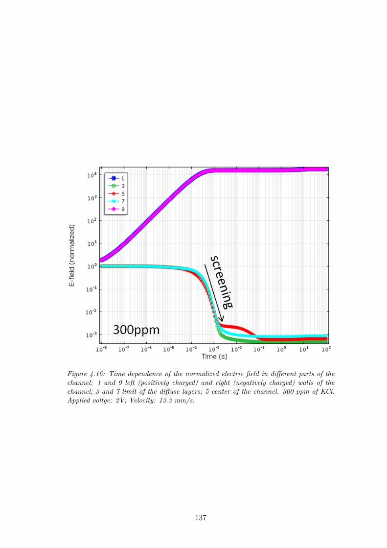
Figure 4.16: Time dependence of the normalized electric field in different parts of thechannel: 1 and 9 left (positively charged) and right (negatively charged) walls of thechannel; 3 and 7 limit of the diffuse layers; 5 center of the channel. 300 ppm of KCl.Applied voltge: 2V; Velocity: 13.3 mm/s.

137

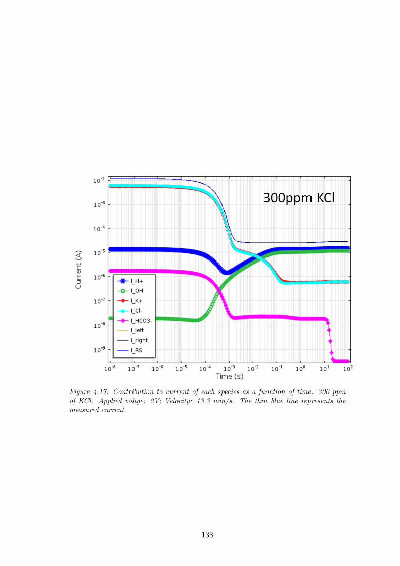
Figure 4.17: Contribution to current of each species as a function of time. 300 ppmof KCl. Applied voltge: 2V; Velocity: 13.3 mm/s. The thin blue line represents themeasured current.

138

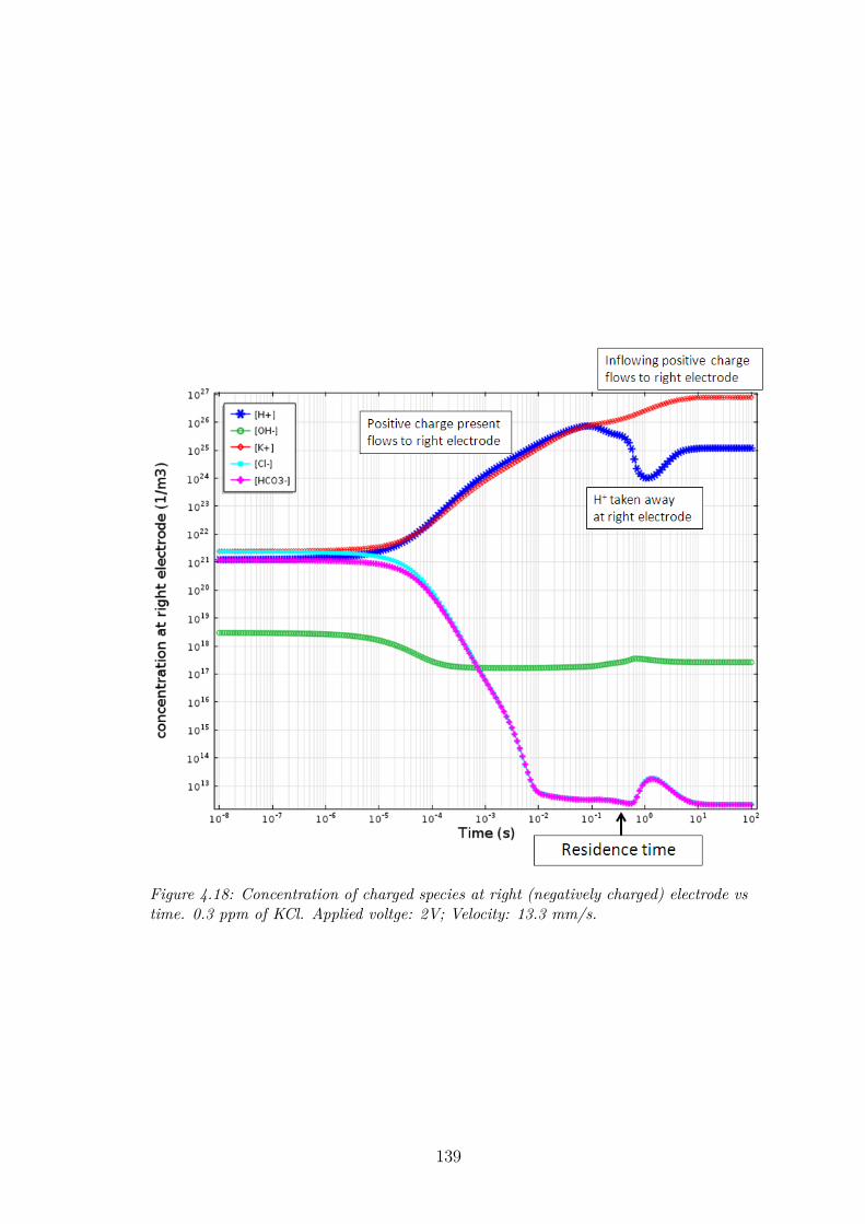
Figure 4.18: Concentration of charged species at right (negatively charged) electrode vstime. 0.3 ppm of KCl. Applied voltge: 2V; Velocity: 13.3 mm/s.

139

Figure 4.19: Steady-state concentration profile within the cell gap of each chargedspecies. 300 ppm of KCl. Applied voltge: 2V; Velocity: 13.3 mm/s.

140

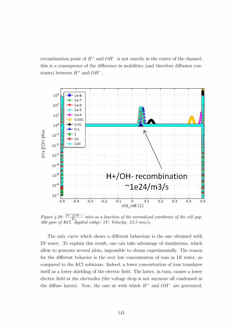
recombination point of H+ and OH− is not exactly in the center of the channel;this is a consequence of the difference in mobilities (and therefore diffusion con-stants) between H+ and OH−.

Figure 4.20: [H+][OH−]Kw

ratio as a function of the normalized coordinate of the cell gap.300 ppm of KCl. Applied voltge: 2V; Velocity: 13.3 mm/s.

The only curve which shows a different behaviour is the one obtained withDI water. To explain this result, one can take advantage of simulations, whichallow to generate several plots, impossible to obtain experimentally. The reasonfor the different behavior is the very low concentration of ions in DI water, ascompared to the KCl solutions. Indeed, a lower concentration of ions translatesitself as a lower shielding of the electric field. The latter, in turn, causes a lowerelectric field at the electrodes (the voltage drop is not anymore all condensed inthe diffuse layers). Now, the rate at with which H+ and OH− are generated,

141

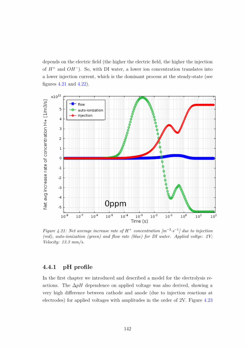
depends on the electric field (the higher the electric field, the higher the injectionof H+ and OH−). So, with DI water, a lower ion concentration translates intoa lower injection current, which is the dominant process at the steady-state (seefigures 4.21 and 4.22).

Figure 4.21: Net average increase rate of H+ concentration [m−3·s−1] due to injection(red), auto-ionization (green) and flow rate (blue) for DI water. Applied voltge: 2V;Velocity: 13.3 mm/s.

4.4.1 pH profile

In the first chapter we introduced and described a model for the electrolysis re-actions. The ∆pH dependence on applied voltage was also derived, showing avery high difference between cathode and anode (due to injection reactions atelectrodes) for applied voltages with amplitudes in the order of 2V. Figure 4.23

142

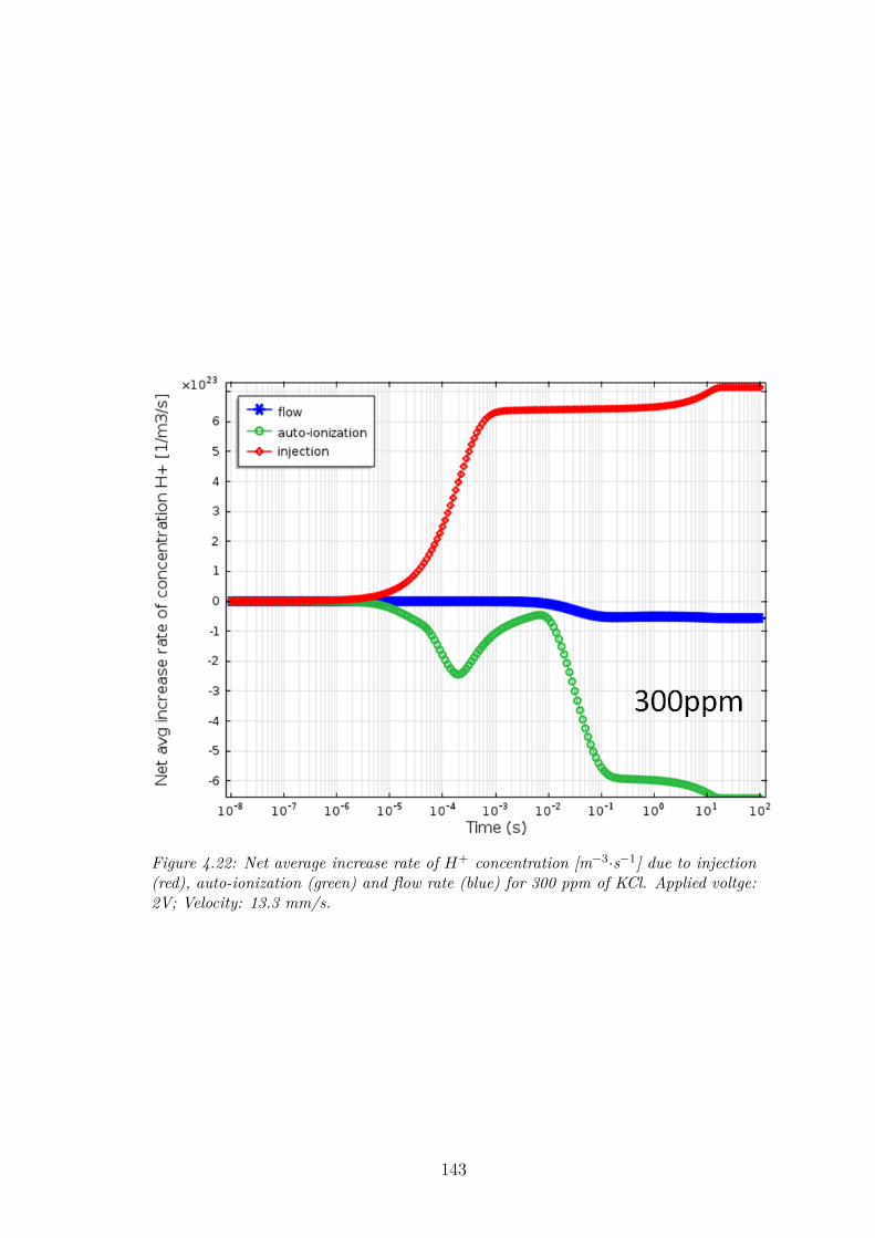
Figure 4.22: Net average increase rate of H+ concentration [m−3·s−1] due to injection(red), auto-ionization (green) and flow rate (blue) for 300 ppm of KCl. Applied voltge:2V; Velocity: 13.3 mm/s.

143

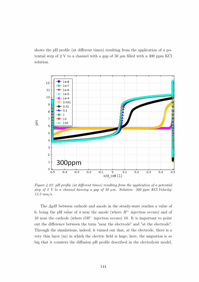
shows the pH profile (at different times) resulting from the application of a po-tential step of 2 V to a channel with a gap of 50 µm filled with a 300 ppm KClsolution.

Figure 4.23: pH profile (at different times) resulting from the application of a potentialstep of 2 V to a channel haveing a gap of 50 µm. Solution: 300 ppm KCl.Velocity:13.3 mm/s.

The ∆pH between cathode and anode in the steady-state reaches a value of6, being the pH value of 4 near the anode (where H+ injection occurs) and of10 near the cathode (where OH− injection occurs) 10. It is important to pointout the difference between the term "near the electrode" and "at the electrode".Through the simulations, indeed, it turned out that, at the electrode, there is avery thin layer (m) in which the electric field is huge; here, the migration is sobig that it counters the diffusion pH profile described in the electrolysis model,

144

thus becoming the dominant transport process. Following this insight, the pH atanode is almost 10 (while near anode, as in the electrolysis model, pH=4), and atcathode its value is 2 (while near cathode, as in the electrolysis model, pH=10).Note that the pH profile obtained in section 1.2.3 doesn’t take into account forthe difference between pH at the electrodes and pH near the electrodes.TheH+ and OH− generation at anode and cathode is basically determined by thescreening, which modifies the electric field profile in such a way that all appliedvoltage is condensed in the diffuse layers at the electrodes, thus giving the neededenergy to drive the injection reactions. So, the accumulation of K+ at negativelycharged electrode, and of Cl− at positively charged electrode, is the process thatdetermines the amount of H+ and OH− created, and so the external current thatflows within the system.

4.5 Conclusions and outlook

In the present work two main results have been discussed: (i) an experimentalinvestigation of the material which shows the best performance (occurrence ofelectrolysis at highest applied voltage), and (ii) an experimental and numericalcharacterization of the electrochemical and transport picture occurring in flow-through microsized devices.

For the first part, we have conducted experiments using Elctrochemical ImpedanceSpectroscopy to first characterize all samples, and then Potential step voltamme-try measurements to probe the external current as a function of time; in bothexperiments, aqueous solution with different concentrations of KCl have beenused (0, 3, 30, 300 ppm). Through EIS, we apply an external alternate (sinu-soidal) 50 mV voltage, in a very wide frequency range (1MHz to 10mHz), betweenthe electrodes whereby two main electrokinetic effects are induced in the system:(i) electric double layer at both the electrodes, (ii) electrode polarization capac-ity at low frequency. To fit the measured data, an equivalent electrical network,in which each element has a physical origin, has been developed. We observea characteristic low frequency high capacitance behaviour which turned out tobeindependent on concentrations of KCl, flow rate, and pH; the only dependence

145

is on electrode material, thus suggesting that this behaviour can be generatedby an adsorption process. By means of Potential Step Voltammetry, we obtaina steady-state I-V curve for different materials. As expected from literature, thebest performing material, for our purpose, is the Boron doped diamond, whichby far shows the highest overpotential (4.2V).

For the second part, we report both an experimental and numerical study ofthe I-t curve resulting from the application of a voltage step. An potential stepwith 2V amplitude has been applied to Pt sample, using controlled conditionsof flow rate, and using different concentrations of KCl (0, 3, 30, 300 ppm). Thedynamics of charge transport have been studied reproducing the experimentalconditions in several finite element COMSOL simulations. Most of the effectsoccurring within the channel have been described and explained. A model forthe electrolysis reactions at the electrodes has been developed. We propose anelectrochemical analysis of reactions at the electrodes at different applied voltages(from ∆V < 0.61 to ∆V > 2). Four regimes turn out, which are in qualitativeagreement with experimental data. Futhermore, this model predict an interestingpicture, involving a pH dependence on applied voltage, which is also confirmed bysimulations. A detailed experimental study of the effect of the flow on the steady-state current have been developed; the results shows a negligible dependencein the experiments with aqueous solution with different concentrations of KCl.Nevertheless, by probing the dependence of the current on flow rate using DIwater, an interesting result turned out: the measured current is lower when theflow is on, while increases when it is switched off.

The next step of our research involves experiments on the quantification ofseparation efficency; then the optimization of all parameters, together with thedesign of an appropriate industrial prototype, can lead to the realization of aninnovative product, able to compete with already existing water purification tech-nologies.

146

Appendix A

Figure 24: EIS on Jb34; Capacitance vs Frequency (Blue line: Real C; Red line: Im-maginary C). De-Ionized water (pH 5.7), flowrate 32 µL/min, ∆V=50mV.

147

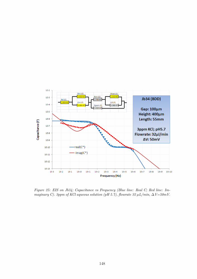
Figure 25: EIS on Jb34; Capacitance vs Frequency (Blue line: Real C; Red line: Im-maginary C). 3ppm of KCl aqueous solution (pH 5.7), flowrate 32 µL/min, ∆V=50mV.

148

Figure 26: EIS on Jb34; Capacitance vs Frequency (Blue line: Real C; Red line: Immag-inary C). 30ppm of KCl aqueous solution (pH 5.7), flowrate 32 µL/min, ∆V=50mV.

149

Figure 27: EIS on Jb34; Capacitance vs Frequency (Blue line: Real C; Red line: Immag-inary C) . 300ppm of KCl aqueous solution (pH 5.7), flowrate 32 µL/min, ∆V=50mV.

150

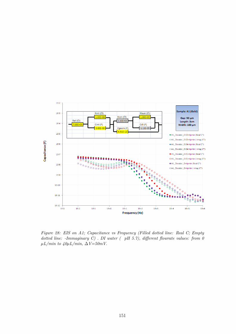
Figure 28: EIS on A1; Capacitance vs Frequency (Filled dotted line: Real C; Emptydotted line: -Immaginary C) . DI water ( pH 5.7), different flowrate values: from 0µL/min to 40µL/min, ∆V=50mV.

151

Appendix B

152

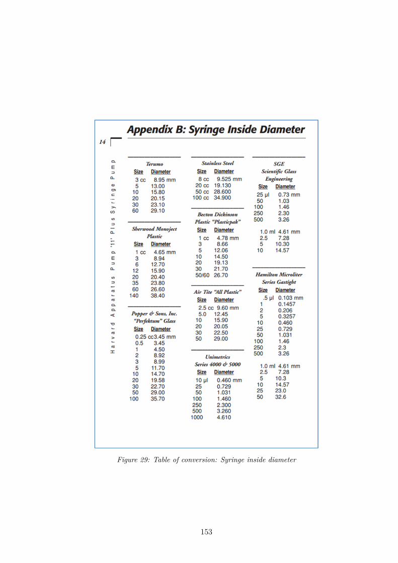
Figure 29: Table of conversion: Syringe inside diameter

153

Appendix C

154

Figure 30: Table of conversion: Flow rate

155

Bibliography

[1] Gouy, L. G. Comt.Rend. 149, 654 (1909), J.Phys. 4, 9, 457 (1910). 1

[2] Chapman, D.f Phil.Mag., 6, 25, 475 (1913). 1

[3] A.R.M. Verschueren et. al Screening and Separation of Charges in MicroscaleDevices: Complete Planar Solution of the Poisson-Boltzmann Equation, J.Phys. Chem. B 2008, 112, 13038–13050. xvii, 1, 9, 13

[4] Filip Beunis, Filip Strubbe, Matthias Marescaux, Jeroen Beeckman, Kristi-aan Neyts and Alwin RM Verschueren Dynamics of charge transport in pla-nar devices, Physical Review E, Vol. 78(1), pp. 011502-1-011502-15, 2008. 1,66

[5] Alwin RM Verschueren, R. A. H. Niessen, P. H. L. Notten, W. Oepts andE. M. L. Alexander-Moonen Experiments and Modeling of Conduction andCharge Accumulation in Liquid Crystal Cells, IEEE Transactions on Di-electrics and Electrical Insulation Vol. 10, No. 6; December 2003. 40

[6] J.R. Macdonald, W.B. Johnson Impedance Spectroscopy, John Wiley & Sons,2005. 57

[7] Andrzej Lasia Electrochemical Impedance Spectroscopy and its Applications,Kluwer Academic/Plenum Publishers, New York, 1999, Vol. 32, p. 143-248.57

[8] Truman S. Light, Stuart Licht, Anthony C. Bevilacqua and Kenneth R.Morash The Fundamental Conductivity and Resistivity of Water, Electro-chemical and Solid-State Letters, 8 (1) E16-E19, 2005. 21

156

[9] Marek Szklarczyk, Ramesh C. Kainthla, and John O’M. Bockris On the Di-electric Breakdown of Water: An Electrochemical Approach, J. Electrochem.Soc., Vol. 136, No. 9, September 1989. 24

[10] Natzle, Wesley C.; Moore, C. Bradley Recombination of hydrogen ion (H+)and hydroxide in pure liquid water, The journal of physical chemistry, Amer-ican Chemical Society, 1985. 23

[11] G. Barbero and A.L. Alexe-Ionescu Role of the diffuse layer of the ioniccharge on the impedance spectroscopy of a cell of liquid, Liquid Crystals,Vol. 32, No. 7, July 2005, 943-949. 43

[12] Laurits Højgaard Olesen, Martin Z. Bazant, and Henrik Bruus Strongly non-linear dynamics of electrolytes in large ac voltages, Physical Review E 82,011501; 2010. 57

[13] R.D. O’Neill, Seung-Cheol Chang, J.P. Lowry, C.J. McNeil Comparison ofPt, Au, Pd and glassy carbon as electrode materials in the design of biosen-sors for glutamate, Elsevier, Biosensors & Bioelectronics, 19 (2004). 1521-1528. 127

[14] Alexander Kraft Doped Diamond: A Compact Review on a New, VersatileElectrode Material, Int. J. Electrochem. Sci., 2 (2007) 355 - 385. 127

[15] J.Rossmeisl, A.Logadottir, J.K. Norskov Electrolysis of water on (oxidized)metal surfaces, Elsevier, Chemical Physics, 319 (2005) 178-184. 24

[16] N.F. Mott, R.J. Watts-Tobin The interface between a metal and an elec-trolyte, Electrochemica Acta, 1961, Vol. 4, pp. 79 to 107. 24

[17] Erich W. Tiepell and Keith E. Gubbins Thermodynamic Properties of GasesDissolved in Electrolyte Solution, Ind. Eng. Chem. Fundam., Vol. 12, NO. 1,1973 27

[18] Henrik Bruus Theoretical Microfluidics, Oxford Master Series in CondensedMatter Physics, Oxfor University Press (2008) viii, 18, 19

157

[19] William Shockley Currents to Conductors Induced by a Moving PointCharge, Journal of Applied Physics 9 (10): 635 (1938) 53

[20] Simon Ramo Currents Induced by Electron Motion, Proceedings of the IRE27 (9): 584–585. (1939) 53

158