CHARACTERIZATION OF SWELLING STRESS AND SOIL ...

CHARACTERIZATION OF SWELLING STRESS AND SOIL MOISTURE DEFICIENCY RELATIONSHIP FOR

EXPANSIVE UNSATURATED SOILS

by

ARMAND AUGUSTIN FONDJO TAKOUKAM

A dissertation submitted in fulfilment of the requirements for the degree

Master of Engineering in Civil Engineering

in the

Department of Civil Engineering

of the

Faculty of Engineering, Built Environment and Information Technology

of the

Central University of Technology, Free State, South Africa

Supervisor: Prof, E. Theron

June 2018

© Central University of Technology, Free State

ii

DECLARATION

I, the undersigned, declare that the dissertation hereby submitted by me for the

degree Master of Engineering in Civil Engineering at the Central University of

Technology, Free State, is my own independent work and has not been submitted

by me to another University and/or Faculty in order to obtain a degree. I further

cede copyright of this dissertation in favour of the Central University of

Technology, Free State.

Armand Augustin Fondjo Takoukam

Signature

Signature:

Date: June 2018

Bloemfontein, South Africa


iii

ABSTRACT Expansive soils vary in volume, in relation to water content. Volume changes when

wetting (swelling) and drying (shrinkage). Lightweight structures in construction are

the most vulnerable structures experiencing severe defects when built on these

soils. In South Africa, expansive soils are the most problematic which impose

challenges to civil engineers. The prediction of the swelling stress has been a

concern to the construction industry for a long time. The swelling stress is

generally ignored in engineering practice. Nonetheless, the swelling stress can

develop significant uplift forces detrimental to the stability of foundations.

Considering the swelling stress in foundation design in expansive soils enhance

the durability, the service life, and reduce the cost of assessment and repair works

to be undertaken in the future. Mathematical models are offered as an alternative

to direct oedometer testing. Mathematical models are a useful tool to assess

swelling stress.

The aim of this study was to characterize the relationship between the swelling

stress, the soil suction, and other soil parameters. Moreover, develop

mathematical models to predict the swelling stress of field compacted expansive

soils. Laboratory tests have been performed such as particle size distribution,

Atterberg limits, linear shrinkage, specific gravity, free swell ratio, X-ray diffraction,

soil suction measurement, modified Proctor compaction test, and zero-swell test

(ZST). Multiple regression analysis was performed using software NCSS11 to

analyze the data obtained from the experiments. The relationships between the

swelling stress and other soil parameters were established. It was observed that,

at the optimum moisture content (OMC), the swelling stress values are within the

range of 48.88 kPa to 261.81 kPa, and the matric suction values are within the

range of 222.843 kPa to 1,778.27 kPa. The swelling stress values on the dry side

of the OMC are higher than values on the wet side. In addition, compaction at the

OMC can reduce the swelling stress by 15%. Furthermore, the geotechnical index

properties, the swelling parameters, affect the swelling stress of compacted

expansive soils. Nevertheless, there is a key impact of the type of clay mineral on

swelling stress.


iv

Six predictive mathematical models were developed. These models were validated

using soil samples collected from various areas across the province of Free State

(Petrusburg, Bloemfontein, Winburg, Welkom, and Bethlehem).

Lastly, good correlations between predicted values and values obtained from

experimental works confirm the reliability of the multiple regression analysis. The

data points are very close to the line 1:1. Furthermore, the graphical analysis

shows that the correlation of the values obtained from the models developed in

this study are more precise than the values obtained from other models.

Therefore, the predictive models developed in this research work are capable to

estimate the swelling stress with acceptable accuracy.

Keywords: Compaction, expansive soils, filter paper, soil parameters, smectite,

soil suction, swelling stress.


v

RESUME

Les sols expansifs sont ces sols qui changent de volume en fonction de leur

teneur en eau. Leur volume augmente suite à l'augmentation de la teneur en eau,

et diminue avec la réduction de la teneur en eau, suivi de la dessiccation lorsqu’ ils

sont asséchés. Les constructions légères sont plus exposées aux dégâts

engendrés par les sols expansifs. En Afrique du Sud, les sols expansifs sont

considérés comme les plus problématiques. La problématique des sols expansifs

est un défi à relever par les ingénieurs du génie civil. La prédiction de la pression

de gonflement a longtemps été une préoccupation importante dans l’industrie de la

construction. La pression de gonflement est généralement ignorée dans la

pratique. Cependant, cette pression est capable de développer des forces de

soulèvement destructrices pour les fondations. La considération de la pression de

gonflement dans le calcul des fondations améliore la durée de vie des ouvrages,

réduit les coûts onéreux d’évaluations et de réparations. Les modèles développés

dans cette étude sont une alternative à L’essai œdométrique direct, et peuvent

être utiliser pour évaluer la pression de gonflement des sols expansifs.

Le but de cette recherche était de caractériser la relation entre la pression de

gonflement, la succion du sol, et les autres paramètres de sol. Ensuite, proposer

des modèles pour prédire la pression de gonflement des sols. Plusieurs tests de

laboratoire ont été réalisés, notamment l’analyse granulométrique, limites

d’Atterberg, limite au retrait, gravité spécifique, l'Indice de gonflement libre, ratio

du gonflement libre, l’analyse minéralogique par diffraction au rayon X, la mesure

de la succion de soil, l’essai de compactage, et la mesure de la pression de

gonflement à volume constant. L’analyse des données expérimentales obtenues

des essais de laboratoire ont été conduite par l’analyse par régression multiple

avec l’outil logiciel NCSS11. Plusieurs corrélations entre la pression de

gonflement, la succion de sol, et les autres paramètres de sol ont été établies. A la

teneur en eau optimale, la pression de gonflement varie de 48.88kPa à 261.81

kPa, et la succion matricielle de 222.843 kPa à 1778.27kPa. Les valeurs de la

pression de gonflement du côté sec de la teneur en eau optimale sont supérieures

à celle obtenues du côté humide. Par ailleurs, le compactage des sols expansifs à

la teneur en eau optimale réduit la pression de gonflement d’environ 15%. En


vi

dehors de la succion matricielle, plusieurs autres paramètres de sol influencent la

pression de gonflement. Cependant, le type de minéral argileux a une influence

importante sur la pression de gonflement.

Six modèles pour prédire la pression de gonflement ont été proposés. Ces

modèles ont été validés sur des sols prélevés dans cinq villes de la province de

Free State à savoir : Petrusburg, Bloemfontein, Winburg, Welkom, et Bethlehem.

De très bonne corrélations ont été établies entre les données expérimentales et

celle obtenues des modèles proposés. Les données graphiques de ces

corrélations sont très proche de la ligne 1:1. Aussi, la comparaison des valeurs

obtenues des modèles développés dans cette étude avec les valeurs obtenues

des autres modèles existants montre que les modèles proposés dans cette étude

donnent une meilleure corrélation. En conclusion, les modèles développés dans

cette étude sont capables de prédire la pression de gonflement avec une précision

acceptable.

Mots clés: Compactage, sol expansifs, papier filtre, paramètres de sol,

montmorillonite, succion de sol, pression de gonflement.


vii

ACKNOWLEDGEMENTS

A number of special acknowledgements deserve specific mention:

(a) The Rectorate and relevant functionaries from the Central University of

Technology, Free State, for the opportunity of completing this research;

(b) The various agencies for funding and in particular the Central University of

Technology, Free State;

(c) Pr. E, Theron my supervisor, for guidance and support given;

(d) My family and colleagues, for their patience and understanding throughout

this research; and

(e) My wife and our children for their love and support.

Acknowledgement above all to my Heavenly Father for setting my feet on a rock

and making my steps secure (Ps. 40).


viii

TABLE OF CONTENTS

Page

Declaration .............................................................................................................. ii

Abstract .................................................................................................................. iii

Résumé ................................................................................................................... v

Acknowledgements ............................................................................................... vii

Table of Contents ................................................................................................. viii

List of Tables ........................................................................................................ xiv

List of Figures ........................................................................................................ xv

List of Appendices ................................................................................................ xxi

List of Abbreviations ............................................................................................ xxiii

Notations and Symbols ...................................................................................... xxiv

CHAPTER 1 : INTRODUCTION ............................................................................. 1

1.1 Background ....................................................................................................... 1

1.2 Problem statement ............................................................................................ 2

1.3 Research objective ............................................................................................ 3

1.4 Research scope ................................................................................................ 4

1.5 Dissertation layout ............................................................................................. 4

CHAPTER 2 : LITERATURE REVIEW ................................................................... 5

PART 1: EXPANSIVE SOILS ................................................................................. 5

2.1 Definition ........................................................................................................... 5

2.2 Origin ................................................................................................................. 5

2.3 Climate .............................................................................................................. 6

2.4 Topography ....................................................................................................... 6

2.5 Time .................................................................................................................. 6

2.6 Mineralogical composition of clays .................................................................... 7

2.6.1 Kaolinte ................................................................................................ 7

2.6.2 Illite ...................................................................................................... 7

2.6.3 Montmorillonite ..................................................................................... 7

2.7 Assessment and classification of expansive soils ............................................. 9

2.7.1 Laboratory testing .............................................................................. 10

2.7.2 Particle size distribution ..................................................................... 10


ix

2.7.3 Atterberg limit ..................................................................................... 10

2.7.4 Mineralogical testing .......................................................................... 12

2.8 Swell potential testing (indirect measurement)................................... 12

2.8.1 Expansive capacity classification based on plasticity table ................ 12

2.8.2 Swelling capacity classification based on advanced physical

proporties of soils ............................................................................. 12

2.8.3 Casangrade's chart plasticity for swelling potential

classification ...................................................................................... 14

2.9 Swell potential testing (Direct measurement) ..................................... 14

2.9.1 Free swell test .................................................................................... 14

2.10 Site investigation ................................................................................ 15

2.11 In situ testing ...................................................................................... 16

2.12 Classification of expansive soils ......................................................... 16

2.13 Mechanism of swelling ....................................................................... 17

2.14 Factor affecting swell/ shrink behaviour of soil ................................... 18

PART 2: UNSATURATED SOIL MECHANICS .................................................... 20

2.15 Introduction .................................................................................................... 20

2.16 Unsaturated soil mechanics domains application .......................................... 22

2.17 Phase of unsaturated soils ........................................................................... 22

2.17.1 Contractile skin ( Air water interface) ............................................... 23

2.17.2 Water phase ..................................................................................... 24

2.17.3 Air phase .......................................................................................... 24

2.17.4 Solid phase ...................................................................................... 24

2.18 Surface tension ............................................................................................. 25

2.19 Capillary phenomenon................................................................................... 27

2.20 Capillary Height ............................................................................................. 28

2.21 Capillary pressure ......................................................................................... 29

2.22 Theory of soil suction..................................................................................... 31

2.23 Components of soil suction ........................................................................... 32

2.24 Unsaturated soil stress state variables .......................................................... 34

2.24.1 Equilibrium analysis ......................................................................... 34

2.24.2 Stress state variables ....................................................................... 36

2.24.3 Other combination of stress state variables ..................................... 37


x

2.25 Soil water characteristic curve ....................................................................... 37

CHAPTER 3 : PREVIOUS STUDIES ON PREDICTION OF THE SWELL

STRESS ................................................................................................................ 41

3.1 Introduction ...................................................................................................... 41

3.2 Swelling stress ................................................................................................ 41

3.2.1 Definition ............................................................................................ 41

3.3 Swelling stress prediction based on oedometer tests ........................ 41

3.3.1 Technique 1 ....................................................................................... 42

3.3.2 Technique 2 ....................................................................................... 42

3.3.3 Technique 3 ....................................................................................... 43

3.4 Proposed models to predict the swelling stress .................................... 44

3.5 Conclusion ....................................................................................................... 49

CHAPTER 4: EXPERIMENTAL STUDY ............................................................. ..50 4.1 Introduction ...................................................................................................... 50

4.2 Sample location ............................................................................................... 50

4.3 Laboratory tests ............................................................................................... 52

4.3.1 Particle size distribution ..................................................................... 52

4.3.2 Sieve analysis .................................................................................... 53

4.3.3 Hydrometer analysis .......................................................................... 53

4.3.4 Atterberg limits ................................................................................... 54

4.3.5 Liquid limit .......................................................................................... 55

4.3.6 Plastic limit ......................................................................................... 57

4.3.7 Plasticity index ................................................................................... 58

4.3.8 Linear shrinkage test .......................................................................... 58

4.3.9 Specific gravity ................................................................................... 60

4.3.10 Free swell index ............................................................................... 61

4.3.11 Free swell ratio ................................................................................. 63

4.4 X-ray diffraction (XRD) .................................................................................... 64

4.4.1 introduction ........................................................................................ 64

4.4.2 Procedure .......................................................................................... 64

4.5 Modified proctor compaction test ..................................................................... 66

4.5.1 Compaction test procedure ................................................................ 66


xi

4.5.2 Calculation of compaction test parameters ........................................ 70

4.5.3 Plotting of compaction curve .............................................................. 71

4.6 Swelling stress test, experimental procedure and equipment .......................... 72

4.7 Soil suction measurement ............................................................................... 75

4.7.1 Filter paper calibration process .......................................................... 76

4.7.2 Indirect measurement of suction using filter paper ............................ 80

4.8 Multiple regression analysis ............................................................................ 91

4.8.1 Introduction ........................................................................................ 91

4.8.2 Regression analysis process ............................................................ 91

4.8.3 Statement of problem ......................................................................... 91

4.8.4 Selection of relevant variables .......................................................... 91

4.8.5 Data collection .................................................................................. 92

4.8.6 Model specification ........................................................................... 93

4.8.7 Model fitting ........................................................................................ 94

4.8.8 Model validation ................................................................................. 94

CHAPTER 5 : ADVANCED TESTING AND ANALYSIS………..…………..……...96 5.1 Introduction ...................................................................................................... 96

5.2 Soil characteristic properties ........................................................................... 96

5.2.1 Grain size classification analysis ........................................................ 96

5.2.2 Unified soil classification system ........................................................ 98

5.2.3 Linear shrinkage ................................................................................ 99

5.2.4 Specific gravity ................................................................................. 100

5.2.5 Activity of clay .................................................................................. 101

5.2.6 Free swell index results analysis ...................................................... 101

5.2.7 Free swell ratio results analysis ....................................................... 102

5.2.8 Comparison free swell ratio and free swell index test results ........... 103

5.3 X- Ray diffraction results analysis ................................................................. 103

5.3.1 Comparison of the results obtained from X-ray diffraction and

Free swell ratio ............................................................................... 106

5.4 Proctor compaction test results ..................................................................... 106

5.4.1 Compaction curves .......................................................................... 106

5.5 Soil suction test results .................................................................................. 111

5.5.1 Soil suction calibrated curves ........................................................... 112


xii

5.5.2 Analysis and discussion of the relationship between soil

suction and water content .............................................................. 114

5.6 Soil water characteristic curve (SWCC)......................................................... 118

5.6.1 Introduction ...................................................................................... 118

5.6.2 Modelling of SWCC .......................................................................... 118

5.6.3 Analysis and discussion of SWCC ................................................... 119

5.6.4 Soil water characteristic curve fit results .......................................... 120

5.6.5 Soil water characteristic curve fitting parameters and

equations ...................................................................................... 123

5.7 Swelling stress results analysis ..................................................................... 123

5.8 Summary of laboratory results ....................................................................... 125

5.9 Analysis and discussion of the correlation between swelling stress and

soil parameters ......................................................................................... 125

5.9.1 Analysis and discussion of the correlation between swelling

stress and soil suctions .................................................................. 125


stress and initial dry density ........................................................... 127


stress and initial water content ....................................................... 128


stress and plasticity index .............................................................. 130


stress and liquid limit ...................................................................... 130


stress and linear shrinkage ............................................................ 131


stress and activity of clay ............................................................... 132


stress and free swell index ............................................................. 133


stress and free swell ratio .............................................................. 133


stress and clay fraction .................................................................. 134


xiii

5.9.11 Conclusion for analysis and discussion of the correlation

between swelling stress and soil properties ................................... 135

5.10 Constitutive models to predict the swelling stress ....................................... 136

5.10.1 Determination of the constitutive models, multi-regression

analysis coefficients, intercepts, and regression statistics ............. 136

5.11 Validation of the models .............................................................................. 138

5.11.1 Model validation by comparing predicted swelling stress

values to the values obtained from experimental works ................. 138

5.11.2 Model validation by comparing the predicted values of

swelling stress to the results obtained from other existing

models ........................................................................................... 141

CHAPTER 6 : CONCLUSION AND PERSPECTIVES…………………...………..145 6.2 Summary ....................................................................................................... 145

6.2 Conclusions ................................................................................................... 145

6.3 Perspectives .................................................................................................. 146

REFERENCES .................................................................................................... 147


xiv

LIST OF TABLES

Page

Table 2.1: Residual soils prone to expansiveness, department of local government,housing and works (1990) .............................................. 6

Table 2.2: Some of clay mineral characteristics (Mitchell, 1993) ........................ 8 Table 2.3: Classification for shrink-swell clay soils (BRE, 1990) ....................... 11 Table 2.4: Potential swell based on plasticity (Hollz & Gribbs, 1956) ............... 12 Table 2.5: Specific gravity of several minerals (Lambe & Whitman,1979) ........ 25 Table 2.6: Surface tension of contractile skin at several temperatures

(Kaye and Laby, 1973) ..................................................................... 26

Table 2.7: Possible combination of stress state variables for

unsaturated soil (Fredlund & Hasan, 1979) ..................................... 37 Table 3.1: Models to predict the swelling stress ............................................... 44 Table 3.2: Models to predict the swelling stress ............................................... 44

Table 4.1: Summary of test standards .............................................................. 52 Table 4.2: Classification of soils base on FSR (Sridharan & Prakash, 2000) ... 63

Table 4.3: Relative density of water according to temperature ......................... 67 Table 4.4: Summary of suction measurement methods .................................... 75 Table 4.5: Total suction of Nacl at 20oC (Lang, 1967) ...................................... 76

Table 4.6: Equilibration times for filter paper method (Leong, 2002) ................ 84

Table 4.7: Regression analysis data ................................................................. 92 Table 4.8: List of variable statistical models and their regression equations.... 94


xv

LIST OF FIGURES

Page

Figure 1.1: Regional distribution map of clay in South Africa (Diop,2011) ........... 1

Figure 1.2: Structural defects caused by expansive soil in Free State ................. 2

Figure 2.1: Diagram of the structure of (a) kaolinite; (b) illite; (c)

montmorillonite ................................................................................... 8

Figure 2.2: Clay mineral layers (Odom, 1984) ..................................................... 9

Figure 2.3: Tetrahedral and octahedral sheets (Odom, 1984) ............................. 9

Figure 2.4: Grain size distribution for dry and wet sieve analysis ....................... 10

Figure 2.5: Relationship in Atterberg limits ......................................................... 11

Figure 2.6: Chart for evaluation of potential expansiveness (Seed et

al.,1975) ........................................................................................... 13

Figure 2.7: Classification chart for swelling potential by carter and

Bentley (1991) .................................................................................. 13

Figure 2.8: Plot of clay mineral on casangrande's chart (Chleboard et al.,

2005) ................................................................................................ 14

Figure 2.9: Phase diagrams of free swell ........................................................... 15

Figure 2.10: Expansive soil, polygonal making of shrinkage fissures on

the surface of the soil ....................................................................... 16

Figure 2.11: Presentation of diffuse double layer and force of attraction.. .......... 17

Figure 2.12: Swell/shrink mechanism .................................................................. 19

Figure 2.13: Categories of soil mechanics (Fredlund & Rahardjo, 1933) ............. 21

Figure 2.14: Excessively arid and semi-arid regions of the world.(Meigs,

1953; Dregne, 1976; Fredlund & Rahardjo, 1993) ........................... 21

Figure 2.15: Stress distribution of dessication (Fredlund and Rahardjo,

1993) ................................................................................................ 22

Figure 2.16: A component of unsaturated soil with a continuous air phase

(Fredlund and Rahardjo, 1993) ........................................................ 23

Figure 2.17: Rigorous fourth-phase unstaurated soil system (Fredlund and

Rahardjo, 1993) ............................................................................... 24

Figure 2.18: Density distribution over air-water interface (Kyklema, 2000) .......... 24


xvi

Figure 2.19: Surface tension phenomenon on contractile skin. (a)

intermolecular forces at air-water interface and water.

(b) Pressures and surface tension acting on a curved two

dimemsional surface ( Fredlund, 1993) ............................................ 26

Figure 2.20: Surface tension on three-dimension warped membrane

(Fredlund and Rahardjo, 1993) ........................................................ 27

Figure 2.21: Physical model and phenomenon related to capillarity (After

Fredlund, 1993) ................................................................................ 29

Figure 2.22: Relationship of the suction matric to pore size for various

soils .................................................................................................. 30

Figure 2.23: Forces acting on capillary tube (Fredlund, 1993) ............................. 31

Figure 2.24: Thermodynamic equilibrium between relative humidity and

total suction ...................................................................................... 32

Figure 2.25: Total suction and its components: matric and osmotic suction

(After Fredlund, 1993) ...................................................................... 33

Figure 2.26: Normal and shear stresses on a cubical soil element of

infinitesimal dimensions ................................................................... 35

Figure 2.27: The stress state variables for unsaturated soil ................................. 36

Figure 2.28: Typical SWCC for different soil types (Fredlund and Xing,

1994) ................................................................................................ 38

Figure 2.29: Definition of variables associated with the SWCC ........................... 38

Figure 3.1: Deformation versus vertical stress, single point test technique

1 (ASTM-D4546) .............................................................................. 42

Figure 3.2: Deformation versus vertical stress, technique 2 (ASTM-

D4546) ............................................................................................. 43

Figure 3.3: Deformation versus vertical stress, loading after wetting test

technique 3 (ASTM-D4546) ............................................................. 43

Figure 3.4: Relation between suction and swelling stress (Thakur et al.,

2005) ................................................................................................ 46

Figure 4.1: Map showing the location of sampling points .................................... 51

Figure 4.2: Collection of the samples from field sites .......................................... 51

Figure 4.3: (a) Sieve analysis, (b) Agitation of sedimentation cylinder, (c)

Hydrometer analysis ........................................................................ 54

Figure 4.4: Apparatus used for Atterberg limits test. .......................................... 55


xvii

Figure 4.5a: Casagrande liquid limit test. ............................................................. 56

Figure 4.5b: Casagrande liquid limit test results. ................................................. 56

Figure 4.6: Soil crumbles during the plastic limit test. ......................................... 57

Figure 4.7: Apparatus used for linear shrinkage test . ........................................ 58

Figure 4.8: Linear shrinkage test . ...................................................................... 59

Figure 4.9: Dried trough with the material .......................................................... 59

Figure 4.10: A view for soil specific gravity test . ................................................. 61

Figure 4.11: Free swelling test: (a) BTS: Bethlehem soil, (b) WKS:

Welkom soil, (c) PTS: Petrusberg soil, (d) BLS: Bloemfontein

soil, (e) WBS: Winburg soil. ............................................................. 62

Figure 4.12: Sample preparation by front loading for XRD test. ........................... 65

Figure 4.13: Multi-purpose diffractometer (MPD) used for XRD test. ................... 65

Figure 4.14: Philips automated powder diffractometer. ........................................ 65

Figure 4.15: Proctor compaction test. .................................................................. 69

Figure 4.16: Maximum dry density and optimum moisture content

determination through Proctor test. .................................................. 71

Figure 4.17: (a) consolidation cell, (b) saturation of porous stone, (c)

assembled consolidation cell, (d) setup of oedometer for

swelling stress measurement. .......................................................... 73

Figure 4.18: (a) compacted specimens wrapped in airtight plastic bag, (b)

specimens kept in a constant temperature bath, (c)

compacted sample inserts inside a consolidation ring using a

jack.. ................................................................................................ 74

Figure 4.19: A view of a conventional consolidometer setup ............................... 74

Figure 4.20: Total suction calibration test sketch ................................................. 77

Figure 4.21: Filter papers calibration curves (reproduced from ASTM

D5298) ............................................................................................. 78

Figure 4.22: (a) Glass jar, salt solution, plastic support, filter paper and tweezers.

(b) Glass jar filled with salt solution .................................................. 79

Figure 4.23: (a) Plastic support hold filter papers; (b) glass jar close tightly ........ 79

Figure 4.24: Non-contact and contact filter paper technique for measuring

the total and matric suction (1st Step) ............................................... 81

Figure 4.25: Non-contact and contact filter paper technique for measuring

the total and matric suction (2nd Step) .............................................. 81


xviii

Figure 4.26: (a) Preparation of compacted soil sample for suction

measurement ................................................................................... 85

Figure 4.27: Three filter papers placed for matric suction measurement. ........... 86

Figure 4.28: Edges of the sample sealed with electrical tape. ............................ 86

Figure 4.29: (a) plastic ring put on soil specimen, (b) Filter paper carried

using tweezers, (c) Filter paper placed over the ring support

for total suction measurement; (d) sealed glass jar.. ........................ 87

Figure 4.30: Temperature regulatory apparatus. ................................................. 88

Figure 4.31: Moisture tin is weighed before filter paper were taken out

from the jar. ...................................................................................... 88

Figure 4.32: Filter papers are put into labeled moisture tines for suction

measurement ................................................................................... 89

Figure 4.33: (a) oven dried moisture tin, (b) moisture tin put on the metal

block to cool it down quickly ............................................................. 90

Figure 5.1: Grain size distribution curve. ........................................................... 97

Figure 5.2a: Chart-grain size distribution. ........................................................... 97

Figure 5.2b: Chart-grain size distribution. ........................................................... 98

Figure 5.3: Liquid limit versus soil designation. ................................................. 98

Figure 5.4: Plasticity index versus soil designation. .......................................... 99

Figure 5.10: Casagrande plasticity chart. ............................................................ 99

Figure 5.11: Linear shrinkage of soil designation. ............................................. 100

Figure 5.12: Specific gravity of soil designation. ............................................... 101

Figure 5.13: Activity of soil designation. ............................................................ 101

Figure 5.14: Free swell index test results. ......................................................... 102

Figure 5.15: Free swell ratio test results. .......................................................... 103

Figure 5.16: X-ray diffraction pattern (WKS). .................................................... 104

Figure 5.17: X-ray diffraction pattern (BLS)....................................................... 104

Figure 5.18: X-ray diffraction pattern (PTS). ..................................................... 105

Figure 5.19: X-ray diffraction pattern (WBS). .................................................... 105

Figure 5.20: X-ray diffraction pattern (BTS). ..................................................... 106

Figure 5.21: Compaction curve graph ............................................................... 108

Figure 5.22: Compaction curve graph (BTS) ..................................................... 108

Figure 5.23: Compaction curve graph (PTS) ..................................................... 109

Figure 5.24: Compaction curve graph (BLS) ..................................................... 109


xix

Figure 5.25: Compaction curve graph (WBS) ................................................... 110

Figure 5.26: Compaction curve graph (WKS) ................................................... 111

Figure 5.27: Calibrated curve using Whatman No 42 filter paper ...................... 112

Figure 5.28: Calibrated curve and adopted curve graph ................................... 113

Figure 5.29: Measured vs predicted values of suction from calibration

curve .............................................................................................. 113

Figure 5.30: Total suction for soil designation at OMC ..................................... 115

Figure 5.31: Matric suction for soil designation at OMC .................................... 115

Figure 5.32: Osmotic suction for soil designation at OMC ................................ 115

Figure 5.33: Suction versus water content (WKS) ............................................ 116

Figure 5.34: Suction versus water content (WBS) ............................................ 116

Figure 5.35: Suction versus water content (BLS) .............................................. 116

Figure 5.36: Suction versus water content (PTS) .............................................. 117

Figure 5.37: Suction versus water content (BTS) .............................................. 117

Figure 5.38: Total suction versus water content ............................................... 117

Figure 5.39: Matric suction versus water content ............................................. 118

Figure 5.40: Volumetric water content at Air entry value (AEV) ....................... 120

Figure 5.41: Matric suction at Air entry value (AEV) ........................................ 120

Figure 5.42: Soil water characteristic curve for WKS as compacted ................ 121

Figure 5.43: Soil water characteristic curve for WBS as compacted ................ 121

Figure 5.44: Soil water characteristic curve for BLS as compacted ................. 122

Figure 5.45: Soil water characteristic curve for PTS as compacted ................. 122

Figure 5.46: Soil water characteristic curve for BTS as compacted ................. 123

Figure 5.47: Swelling stress for soil designation at OMC ................................. 124

Figure 5.48: Maximum swelling stress for soil designation .............................. 124

Figure 5.49: Swelling stress versus total suction ............................................. 126

Figure 5.50: Swelling stress versus matric suction .......................................... 126

Figure 5.51: Swelling stress versus osmotic suction ........................................ 126

Figure 5.52: Swelling stress versus initial dry density ...................................... 127

Figure 5.53: Swelling stress versus initial dry density at OMC ......................... 128

Figure 5.54: Swelling stress versus initial water content .................................. 129

Figure 5.55: Swelling stress versus optimum water content ............................ 129

Figure 5.56: Swelling stress versus plasticity index at OMC ............................ 130

Figure 5.57: Swelling stress versus liquid limit at OMC ................................... 131


xx

Figure 5.58: Swelling stress versus linear shrinkage at OMC .......................... 132

Figure 5.59: Swelling stress versus activity of clay at OMC ............................. 132

Figure 5.60: Swelling stress versus free swell index at OMC ........................... 133

Figure 5.61: Swelling stress versus free swell ratio at OMC ............................ 134

Figure 5.62: Swelling stress versus clay fraction at OMC ................................ 135

Figure 5.63: Comparison between experimental and predicted values of

swelling stress (model 6) .............................................................. 139











Figure 5.69: Comparison of predicted values of swelling stress from

proposed models, and predictive model by Forouzan (2016) ........ 143


proposed models, and predictive model by Yusuf and Ohran

(2007) ............................................................................................ 143


proposed models, and predictive model by Tu and Vanapalli

(2016) ............................................................................................ 144


xxi

LIST OF APPENDICES

APPENDIX A: Table 5.1: Grain size classification ................................................................... 157

Table 5.2: Unified soil classification system (USCS) ........................................ 157

Figure 5.5: Casagrande liquid limit test (BLS). .................................................. 157

APPENDIX B: Figure 5.6: Casagrande liquid limit test (BTS). .................................................. 158

Figure 5.7: Casagrande liquid limit test (WBS). ................................................. 158

Figure 5.8: Casagrande liquid limit test (PTS). .................................................. 158

APPENDIX C: Figure 5.9: Casagrande liquid limit test (WKS). .................................................. 159

Table 5.3: Linear shrinkage test results ............................................................ 159

Table 5.4: Specific gravity test results ............................................................... 159

APPENDIX D: Table 5.5: Free swell index test results .............................................................. 160

Table 5.6 Classification of soil base on FSI ....................................................... 160

Table 5.7: Free swell ratio test results ............................................................... 160

Table 5.8: Classification of soils based on FSR ................................................. 160

APPENDIX E

Table 5.9: Summary of X-Ray diffraction results ............................................... 161

Table 5.10 Compaction test results .................................................................... 161

Table 5.11: Calibrated curves ............................................................................. 161

APPENDIX F: Table 5.12: Suction test results ........................................................................... 162

APPENDIX G: Table 5.13: Soil water characteristic curve data (WKS) ..................................... 163

Table 5.14: Soil water characteristic curve data (WBS) ..................................... 163

Table 5.15: Soil water characteristic curve data (BLS) ....................................... 163

APPENDIX H: Table 5.16: Soil water characteristic curve data (PTS) ...................................... 164

Table 5.17: Soil water characteristic curve data (BTS) ...................................... 164


xxii

Table 5.18: Summary of SWCC results ............................................................. 164

APPENDIX I: Table 5.19: SWCC fitting parameters and equations for soils WKS & WBS ...... 165

APPENDIX J: Table 5.20: SWCC fitting parameters and equations for soils BLS & PTS ......... 166

APPENDIX K: Table 5.21: SWCC fitting parameters and equations for soils BTS .................... 167

APPENDIX L: Table 5.22: Zero swelling test results ................................................................. 168

APPENDIX M: Table 5.23: Summary of laboratory test results @OMC ..................................... 169

Table 5.24: Summary of laboratory test results .................................................. 169

Table 5.25: Summary of laboratory test results .................................................. 169

APPENDIX N: Table 5.26: Correlation Matrix A......................................................................... 170

APPENDIX O: Table 5.27: Correlation Matrix B......................................................................... 171

Table 5.28: Intercepts, coefficients for regression analysis models ................... 171

Table 5.29: Intercepts, coefficient for regression analysis models ..................... 171

APPENDIX P: Table 5.30: Compaction test data sheet ............................................................. 172

APPENDIX Q: Table 5.31: Measurement of soil suction using filter paper data sheet ............... 173


xxiii

LIST OF ABBREVIATIONS

AIC Akaike Information Criterion

AEV Air Entry Value

ASTM American Society for Testing and Material

BLS Bloemfontein Soil

BTS Bethlehem Soil

CST Consolidation Swelling Test

CH High Plastic Clay

CL Medium Plastic Clay

DOT Double Oedometer Test

FSI Free Swell Index

FSR Free Swell Ratio

FPM Filter Paper Method

GSD Grain size distribution

IS Indian Standards

MFSI Modified Free Swell Index

MPD Multi-Purpose Diffractometer

MSR Mean Square Error

OMC Optimum moisture content

PTS Petrusburg Soil

RSS Residual Sum of Squares

RSD Relative Standard Deviation

SWCC Soil Water Characteristic Curve

TMH Technical Method for Highways

USCS Unified Soil Classification System

VCP Volume Change Potential

XRD X-ray diffraction

WBS Winburg Soil

WKS Welkom Soil

ZST Zero Swelling Test


xxiv

NOTATIONS AND SYMBOLS

Roman letters

af Soil parameter related to the air entry of the soil

Ac Activity of clay

br Beam ratio

C Correction factor

ec Unit electron charge

e Natural constant 2.718

f* Interaction function between the equilibrium of the soil

structure and the equilibrium of the contractile skin

𝐹 Interaction force between water phase and the soil particle in

direction (y)

𝐹 Interaction force between the air phase and the soil particle in

direction (y)

g Gram

Gs Specific gravity

hc Capillary height

Iss Swell-shrink index

K Boltzmann’s constant

Ko Number of estimated parameter

LL Liquid limit

LS Linear shrinkage

m Number of relevant soil parameter

m1 Mass of wet filter paper + cold tare

m2 Mass of wet filter paper + hot tare mass

mf Soil parameter related to the residual water content condition

M Total mass

M1 Empty mass of volumetric flask

M2 Mass of pycnometer + oven dry soil

M3 Mass of pycnometer + oven dry soil + filled water

M4 Mass of pycnometer + filled with water only

Ma Mass of air


xxv

Mw Mass of water

Ms Mass of solids

Mc Mass of the contractile skin

Mf Mass of the dry filter paper

Mi Unit mass of surcharge

Mm Mass of the mould and base plate

Msoil Mass of the dry soil

Mt Mass of the mould, base plate, and wet soil

Mw Mass of water to be added

Mv Mass of water in the filter paper

N Number of blows

n Number of surcharges

nf Soil parameter related to the rate of desaturation

nw Porosity relative to the water phase

nc Porosity relative to the contractile skin

ns Porosity relative to the soil particles

PI Plasticity index

Ps Swelling stress

PL Plastic limit

Pso Intercept on the Ps axis at zero suction value

Q(x) Complementary cumulative normal distribution function

R Radius of the capillary tube

R2 Correlation coefficient

RT Universal gas constant

Rd Relative density of water according to temperature

Rs Sheath radius of curvature/ Radius of curvature of the meniscus

R1,R2 Radius of curvature of warped membrane

S Degree of saturation

Se Effective saturation

t Two layers thicknesses

T Temperature

Tc Cold tare mass

Th Hot tare mass


xxvi

Ts Tension surface

Tk Absolute temperature

Tzy Shear stress on the z-plan in y direction

Ua Pore air pressure

Uw Pore water pressure

𝑢 Partial pressure of pore

𝑢 Saturation pressure of water steam over a flat surface of pure

water at the same temperature

V Total volume

Va Volume of air

Vc Volume of contractile skin

Vd Volume of the soil specimen read from the graduated cylinder

containing distilled water.

Vf Final volume of the specimen

Vi Initial volume of the specimen

Vk Volume of the soil specimen read from the graduated cylinder

containing Kerosene

Vs Volume of solids

Vm Volume of the mould

Vw Volume of water

W Moisture content

W1 Mass of container + wet soil

W2 Mass of container + wet soil

Wc Mass of container

Wf Water content of the filter paper

Wi Initial water content

Wopt Optimum moisture content

Wt Targeted moisture content

Xij Independent variables

Y Dependent variable


xxvii

Greek letters

𝛼 Angle of contact

𝛽 Angle between the tension surface and horizontal

𝜀 Dielectric constant medium

𝜀 Random error representing the discrepancies in the

approximation

𝜂 Electrolyte concentration

𝜈 Cation valence

𝜌 Density of water

𝜌 Soil particle density

𝜓 Total soil suction

𝜓 Matric suction

𝜓 Osmotic suction

𝜏 Shear stress on the plan (y,z), perpendicular to direction (y)

𝜏 Shear stress on the plan (x,y), perpendicular to direction (x)

𝜎 Total normal stress parallel to direction (y)

𝜃 Volumetric water at saturation

𝜃 Residual volumetric water content

𝜃 Volumetric water content

𝛾 Dry density

𝛾 Maximum dry density

𝜆 , 𝜂 , 𝜉 , 𝜁 , 𝛽 , 𝜇 Intercepts

𝜆 , 𝜂 , 𝜉 , 𝜁 , 𝛽 , 𝜇 Multi-regression analysis coefficient

( ) Differential function

𝜙 (𝑥) Normalized form of the cumulative normal distribution

function

𝜙 Internal diameter of the consolidation ring

ΔU Difference in stress on a two - dimension curved arc

ΔV Initial change in volume of a specimen


Chapter 1

1

CHAPTER 1: INTRODUCTION

1.1 Background

Defects on constructions caused by heaving soils were first reported in South

Africa in 1950, particularly in Goldfield Mine Free State. Lightweight structures

such as subsidy houses failed to fulfil their service life and were demolished

prematurely. Lightweight constructions are the most vulnerable to heaving soils

because these structures are less capable to overcome the differential movement.

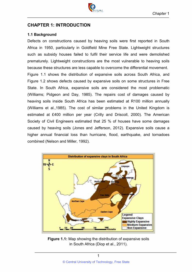
Figure 1.1 shows the distribution of expansive soils across South Africa, and

Figure 1.2 shows defects caused by expansive soils on some structures in Free

State. In South Africa, expansive soils are considered the most problematic

(Williams; Pidgeon and Day, 1985). The repairs cost of damages caused by

heaving soils inside South Africa has been estimated at R100 million annually

(Williams et al.,1985). The cost of similar problems in the United Kingdom is

estimated at £400 million per year (Crilly and Driscoll, 2000). The American

Society of Civil Engineers estimated that 25 % of houses have some damages

caused by heaving soils (Jones and Jefferson, 2012). Expansive soils cause a

higher annual financial loss than hurricane, flood, earthquake, and tornadoes

combined (Nelson and Miller, 1992).

Figure 1.1: Map showing the distribution of expansive soils in South Africa (Diop et al., 2011).


Chapter 1

2

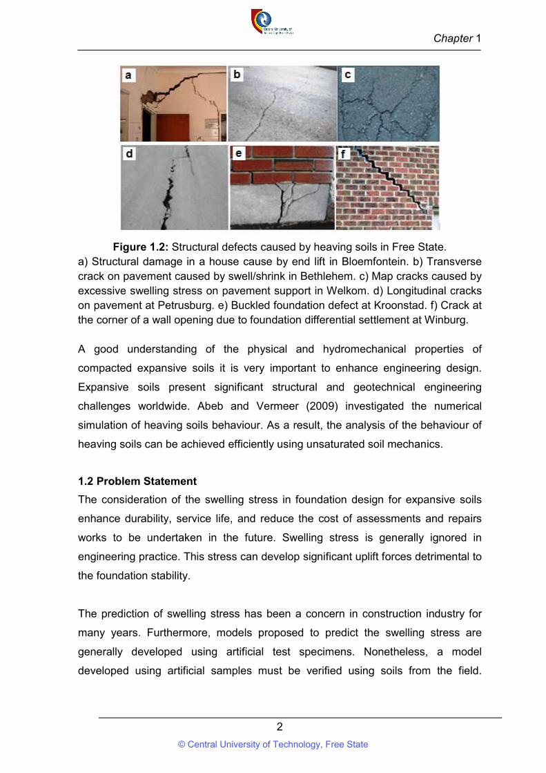
Figure 1.2: Structural defects caused by heaving soils in Free State. a) Structural damage in a house cause by end lift in Bloemfontein. b) Transverse crack on pavement caused by swell/shrink in Bethlehem. c) Map cracks caused by excessive swelling stress on pavement support in Welkom. d) Longitudinal cracks on pavement at Petrusburg. e) Buckled foundation defect at Kroonstad. f) Crack at the corner of a wall opening due to foundation differential settlement at Winburg.

A good understanding of the physical and hydromechanical properties of

compacted expansive soils it is very important to enhance engineering design.

Expansive soils present significant structural and geotechnical engineering

challenges worldwide. Abeb and Vermeer (2009) investigated the numerical

simulation of heaving soils behaviour. As a result, the analysis of the behaviour of

heaving soils can be achieved efficiently using unsaturated soil mechanics.

1.2 Problem Statement

The consideration of the swelling stress in foundation design for expansive soils

enhance durability, service life, and reduce the cost of assessments and repairs

works to be undertaken in the future. Swelling stress is generally ignored in

engineering practice. This stress can develop significant uplift forces detrimental to

the foundation stability.

The prediction of swelling stress has been a concern in construction industry for

many years. Furthermore, models proposed to predict the swelling stress are

generally developed using artificial test specimens. Nonetheless, a model

developed using artificial samples must be verified using soils from the field.


Chapter 1

3

Models developed using field compacted samples could predict more precisely the

swelling stress.

The oedometer swelling test is a commonly used technique to measure the

swelling stress. The oedometer swelling test in engineering practice is

cumbersome and time-consuming, making the test unattractive and not cost-

effective for the low-cost housing project. It becomes important to propose models

to predict the swelling stress to alleviate the need for conducting this test.

Laboratory tests used to measure the soil parameters such as soil suctions,

Atterberg limits, dry density, water content, and free swell ratio, have been well

established with standard guidelines. A correlation between the swelling stress

and these soils parameters can be used to indirectly approximate the swelling

stress for a field compacted expansive soils.

Field conditions are often different from those considered in classical soil

mechanics, and particularly when heaving soils are present. Classical soil

mechanics consider the pore pressures to be negligible. However, for unsaturated

conditions, the true nature of pore pressures is more complex. For expansive soils,

unsaturated conditions may prevail, often creating substantial negative pore

pressures, which work to maintain low void ratios and very little expansion.

Nonetheless, as more moisture is introduced into the soil matrix, the soil expands

significantly with a large magnitude of forces. Adopting the classical approach as

described above fails to consider the true nature of the soil. Therefore, a more

appropriate way to consider such soils is through the application of unsaturated

soil mechanics. By doing so, one may better quantify the swelling stress and its

dependence on soil moisture. This leads to a more realistic approach to foundation

design in expansive soils.

1.3 Research objective

The main objective of this study is to characterize the relationship between the

swelling stress and the soil moisture deficiency for compacted expansive soil.

However, the objectives of this research will further focus on the relationship

between the swelling stress and other soil parameters such as geotechnical index

properties, expansive soil parameters.


Chapter 1

4

1. Undertake a comprehensive review of previous research concerned with

the prediction of swelling stress in expansive soils.

2. Perform laboratory experiments to determine the physical and hydro-

mechanical properties of soil specimens as well as the soil water

characteristic curve.

3. Analyze data obtained from laboratory tests, quantitatively by multiple

regression analysis using software NCSS11. Develop a mathematical

model to predict the swelling stress of compacted expansive soils.

4. Validate the models by comparing predicted values obtained from models

proposed in this study to the values obtained from other models.

1.4 Research scope

The results of this study can be applied to foundation design in heaving soils for

lightweight structure. Other problematic soils encountered in South Africa such as

dolomite, collapsible soils, and soft clay are beyond the scope of this study. The

variability of soil parameters, the difference between field and laboratory

measurements due to scale effect, and the degree of accuracy of laboratory tests

performed make this study a contribution.

1.5 Dissertation layout

The research work is organized into six chapters: Chapter 1 covers the general

background, problem statement, aim, and scope of the research. Chapter 2

presents the expansive soils and the unsaturated soil mechanics. Chapter 3

covers previous research works on the prediction of swelling stress. Chapter 4

describes the experimental study. Chapter 5 focus on advanced testing and

analysis. Chapter 6 presents the conclusion and perspectives.


Chapter 2

5

CHAPTER 2: LITERATURE REVIEW

PART 1: EXPANSIVE SOILS

2.1 Definition

Heaving soils vary in volume in relation to water content. This term is commonly

used to characterize rock or soil material with an important swell/shrink potential.

These soils contained clay minerals that swell as the moisture content increases

and shrink when the moisture content decreases.

2.2 Origin

Heaving soils originate from a combination of processes and conditions. Specific

clay minerals formed with a mineralogical and chemical configuration that attracts

and holds a noteworthy volume of water. The parent rock composition and the

intensity of chemical and physical weathering that the materials are exposed

determine the clay mineralogy and likelihood of heave. Parent materials related to

heaving soils are classified into two categories (Grim, 1968). The first category is

formed by basic igneous rock that is composed of a significant metallic base such

as olivine, amphibole, biotite, and pyroxene. Such rock contains volcanic glass and

basalts. The second category comprises the sedimentary rock that contains

smectite. Shale and clay stones constituents are formed with a varying quantity of

glass and volcanic ash that are weathered to form montmorillonite.

Heaving soils may be either residual or transported materials. In residual soil,

heaving soils originates from in-situ chemical weathering of rock. For transported

soil, heaving soils is removed from its in-situ location by wind, water, gravity or ice

and deposited in a different location (William et al., 1985). Transported soils are as

follows: Alluvium (stream or river), Lacustrine deposits (Originating from a stream

then deposited in lake or still water), Gulley wash (from local catchment and which

contain a variety of heaving soils), Hill wash (from lower velocity sheet wash,

usually with less expansive material). Residual soils are the main source of

expansive soils and are summarized in Table 2.1.


Chapter 2

6

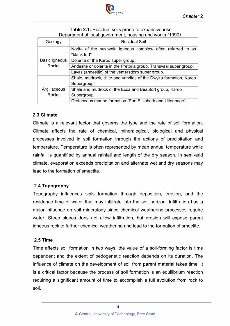
Table 2.1: Residual soils prone to expansiveness Department of local government, housing and works (1990).

Geology Residual Soil

Basic Igneous Rocks

Norite of the bushveld igneous complex- often referred to as "black turf" Dolerite of the Karoo super group. Andesite or dolerite in the Pretoria group, Transvaal super group. Lavas (andesitic) of the ventersdorp super group.

Argillaceous Rocks

Shale, mudrock, tillite and varvites of the Dwyka formation, Karoo Supergroup. Shale and mudrock of the Ecca and Beaufort group, Karoo Supergroup. Cretaceous marine formation (Port Elizabeth and Uitenhage).

2.3 Climate

Climate is a relevant factor that governs the type and the rate of soil formation.

Climate affects the rate of chemical, mineralogical, biological and physical

processes involved in soil formation through the actions of precipitation and

temperature. Temperature is often represented by mean annual temperature while

rainfall is quantified by annual rainfall and length of the dry season. In semi-arid

climate, evaporation exceeds precipitation and alternate wet and dry seasons may

lead to the formation of smectite.

2.4 Topography

Topography influences soils formation through deposition, erosion, and the

residence time of water that may infiltrate into the soil horizon. Infiltration has a

major influence on soil mineralogy since chemical weathering processes require

water. Steep slopes does not allow infiltration, but erosion will expose parent

igneous rock to further chemical weathering and lead to the formation of smectite.

2.5 Time

Time affects soil formation in two ways: the value of a soil-forming factor is time

dependent and the extent of pedogenetic reaction depends on its duration. The

influence of climate on the development of soil from parent material takes time. It

is a critical factor because the process of soil formation is an equilibrium reaction

requiring a significant amount of time to accomplish a full evolution from rock to

soil.


Chapter 2

7

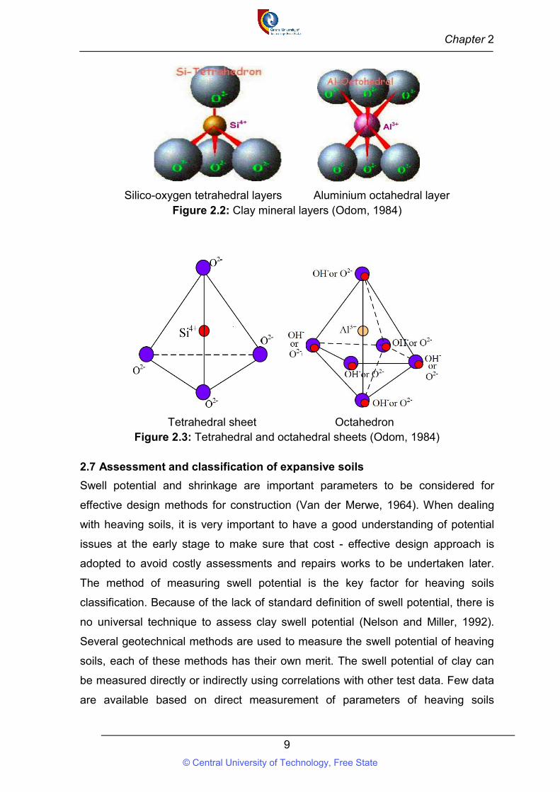
2.6 Mineralogical composition of clays

The structure of the soil is a combination of the effects of the fabrics and

interparticle forces. Holtz et al.,(1981) stated that a soil fabric refers only to the

geometrical arrangement of particles. Clay mineral refer to hydrous aluminum

phyllosilicates minerals that are fine - grained (< 0.002 mm) with a sheet layer

structure and very high surface area (Cameron et al., 1992). Clay minerals are

built up with silicon oxygen tetrahedral (Si4O16)2 layers and aluminum Al12(OH)6

or magnesium Mg3(OH)6, gibbsite or brucite sheet in octahedral layers (Wu, 1978)

as shown in Figures 2.2 and 2.3. Kaolinite group, Illite group, and smectite group

are common clay mineral.

2.6.1 Kaolinite: [Si2Al2O5 (OH)4] is formed with a sequence layer of elemental

silica gibbsite sheets in 1:1 lattice, as shown in Figure 2.1a. Each layer is about

7.2 Å thick. Hydrogen bonding holds layers together. The specific surface of

Kaolinite particle is around 15m2/g. Kaolinite is a non - heaving clay mineral, it will

not crack during drying, instead produces high soil strength.

2.6.2 Illite: [(K,H3O)(Al,Mg,Fe)2(Si,Al)4O10((OH)2,(H2O))] is a clay mineral of 2:1

type mica mineral formed by gibbsite layer bounded to silica layers-one at the

bottom and another at the top as shown in Figure 2.1b. Illite sheets are bonded by

potassium ions. The potassium ions are balanced by negative charge. Potassium

ion comes from the substitution of aluminum for some silicon in tetrahedral sheets.

Illite is not expansive even it is nearly identical to 2:1 phyllosilicate (smectite).

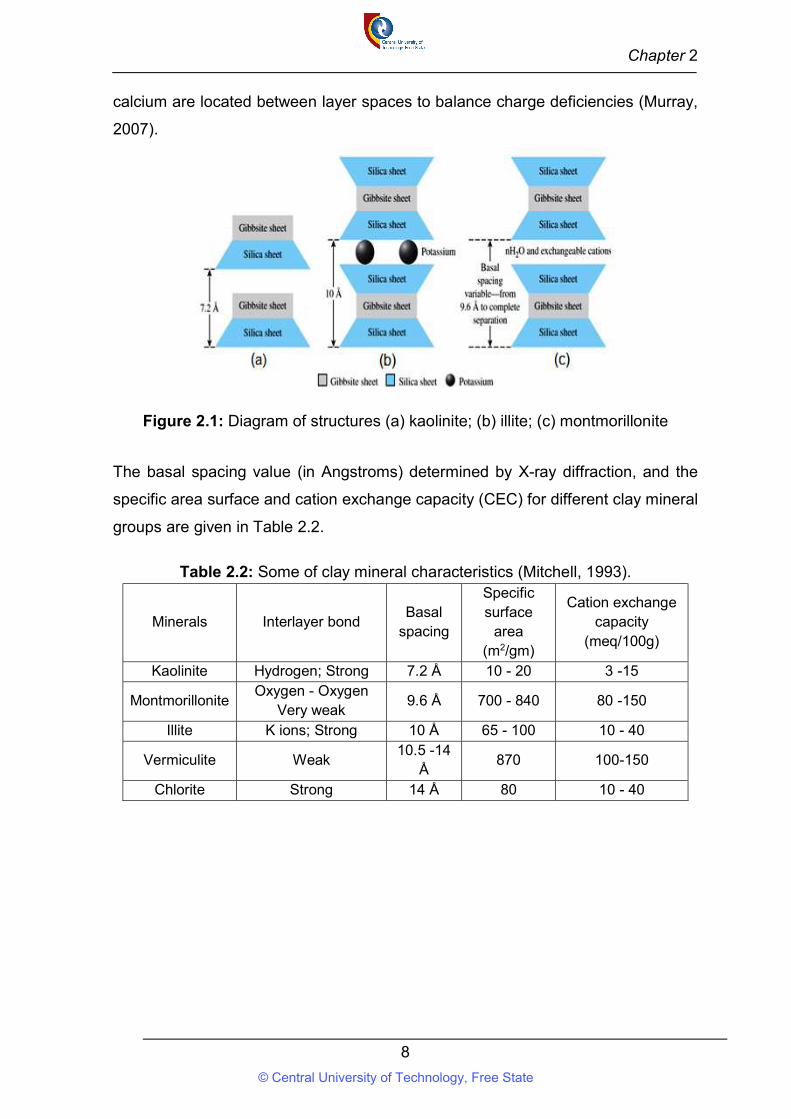
2.6.3 Montmorillonite: [(NaCa)(AlMg)2(Si4O10)(OH)2.nH2O] is the most common

smectite, it is located in arid to the semi - arid climate in which evapotranspiration

exceeds rainfall during the significant period of the year. This is partly explained by

the theory that absence of leaching in moisture deficiency zones helps the

development of montmorillonite (Mitchell, 1993). Montmorillonite structure looks

like that of illite: a gibbsite sheet sandwiched between two silica layers Figure 2.1c.

Montmorillonite contains an isomorphous substitution of magnesium and iron for

aluminum in octahedral layers. Montmorillonite particles have lateral dimensions of

1000 to 5000 Å and thicknesses of 10 to 50 Å. The specific surface is about

800m2/g. A molecule of water and exchangeable cations such as magnesium,


Chapter 2

8

calcium are located between layer spaces to balance charge deficiencies (Murray,

2007).

Figure 2.1: Diagram of structures (a) kaolinite; (b) illite; (c) montmorillonite

The basal spacing value (in Angstroms) determined by X-ray diffraction, and the

specific area surface and cation exchange capacity (CEC) for different clay mineral

groups are given in Table 2.2.

Table 2.2: Some of clay mineral characteristics (Mitchell, 1993).

Minerals Interlayer bond Basal

spacing

Specific surface

area (m2/gm)

Cation exchange capacity

(meq/100g)

Kaolinite Hydrogen; Strong 7.2 Å 10 - 20 3 -15

Montmorillonite Oxygen - Oxygen

Very weak 9.6 Å 700 - 840 80 -150

Illite K ions; Strong 10 Å 65 - 100 10 - 40

Vermiculite Weak 10.5 -14

Å 870 100-150

Chlorite Strong 14 Å 80 10 - 40


Chapter 2

9

Silico-oxygen tetrahedral layers Aluminium octahedral layer Figure 2.2: Clay mineral layers (Odom, 1984)

Tetrahedral sheet Octahedron Figure 2.3: Tetrahedral and octahedral sheets (Odom, 1984)

2.7 Assessment and classification of expansive soils

Swell potential and shrinkage are important parameters to be considered for

effective design methods for construction (Van der Merwe, 1964). When dealing

with heaving soils, it is very important to have a good understanding of potential

issues at the early stage to make sure that cost - effective design approach is

adopted to avoid costly assessments and repairs works to be undertaken later.

The method of measuring swell potential is the key factor for heaving soils

classification. Because of the lack of standard definition of swell potential, there is

no universal technique to assess clay swell potential (Nelson and Miller, 1992).

Several geotechnical methods are used to measure the swell potential of heaving

soils, each of these methods has their own merit. The swell potential of clay can

be measured directly or indirectly using correlations with other test data. Few data

are available based on direct measurement of parameters of heaving soils


Chapter 2

10

because these data are required for a few engineering applications. Nonetheless,

these procedures give a good indicator of expansive potential when the soil is

subjected to laboratory test conditions. Therefore, reliance must be placed on

estimation base on index parameters such as plasticity index, dry density (Reeve

et al., 1980; Holtz and Kovacs, 1981; Oloo et al., 1987).

2.7.1 Laboratory testing

Generally, three different methods are used to assess heaving soils in the

laboratory: index tests, mineralogy test, and swelling-shrinkage test.

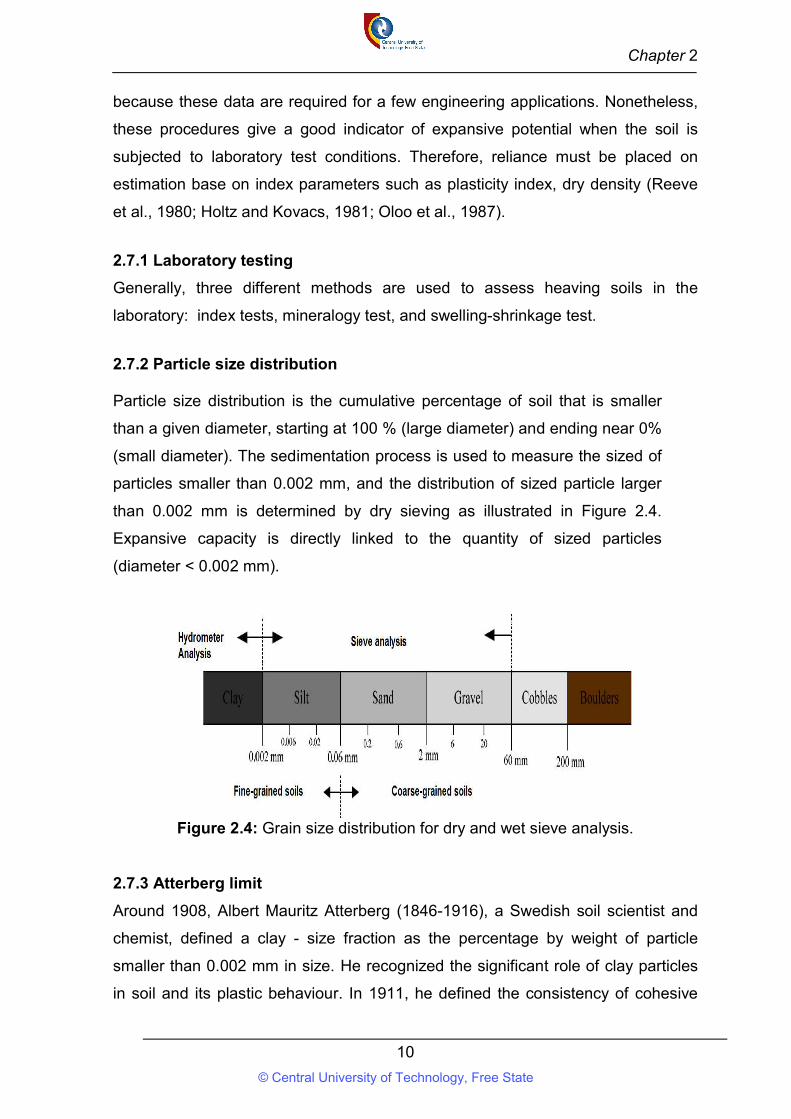
2.7.2 Particle size distribution

Particle size distribution is the cumulative percentage of soil that is smaller

than a given diameter, starting at 100 % (large diameter) and ending near 0%

(small diameter). The sedimentation process is used to measure the sized of

particles smaller than 0.002 mm, and the distribution of sized particle larger

than 0.002 mm is determined by dry sieving as illustrated in Figure 2.4.

Expansive capacity is directly linked to the quantity of sized particles

(diameter < 0.002 mm).

Figure 2.4: Grain size distribution for dry and wet sieve analysis.

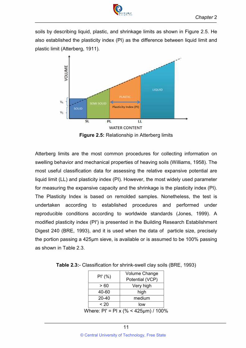
2.7.3 Atterberg limit

Around 1908, Albert Mauritz Atterberg (1846-1916), a Swedish soil scientist and

chemist, defined a clay - size fraction as the percentage by weight of particle

smaller than 0.002 mm in size. He recognized the significant role of clay particles

in soil and its plastic behaviour. In 1911, he defined the consistency of cohesive


Chapter 2

11

soils by describing liquid, plastic, and shrinkage limits as shown in Figure 2.5. He

also established the plasticity index (PI) as the difference between liquid limit and

plastic limit (Atterberg, 1911).

Figure 2.5: Relationship in Atterberg limits

Atterberg limits are the most common procedures for collecting information on

swelling behavior and mechanical properties of heaving soils (Williams, 1958). The

most useful classification data for assessing the relative expansive potential are

liquid limit (LL) and plasticity index (PI). However, the most widely used parameter

for measuring the expansive capacity and the shrinkage is the plasticity index (PI).

The Plasticity Index is based on remolded samples. Nonetheless, the test is

undertaken according to established procedures and performed under

reproducible conditions according to worldwide standards (Jones, 1999). A

modified plasticity index (PI') is presented in the Building Research Establishment

Digest 240 (BRE, 1993), and it is used when the data of particle size, precisely

the portion passing a 425μm sieve, is available or is assumed to be 100% passing

as shown in Table 2.3.

Table 2.3:- Classification for shrink-swell clay soils (BRE, 1993)

PI' (%) Volume Change Potential (VCP)

> 60 Very high 40-60 high 20-40 medium < 20 low

Where: PI' = PI x (% < 425μm) / 100%


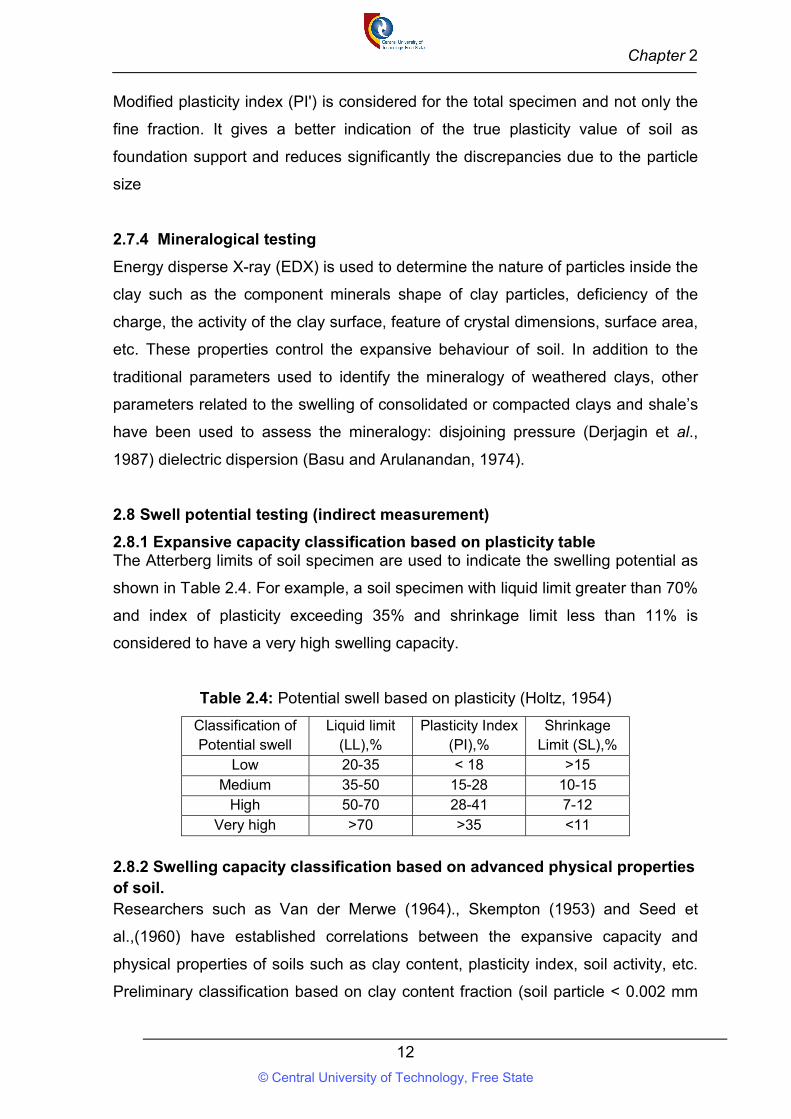
Chapter 2

12

Modified plasticity index (PI') is considered for the total specimen and not only the

fine fraction. It gives a better indication of the true plasticity value of soil as

foundation support and reduces significantly the discrepancies due to the particle

size

2.7.4 Mineralogical testing

Energy disperse X-ray (EDX) is used to determine the nature of particles inside the

clay such as the component minerals shape of clay particles, deficiency of the

charge, the activity of the clay surface, feature of crystal dimensions, surface area,

etc. These properties control the expansive behaviour of soil. In addition to the

traditional parameters used to identify the mineralogy of weathered clays, other

parameters related to the swelling of consolidated or compacted clays and shale’s

have been used to assess the mineralogy: disjoining pressure (Derjagin et al.,

1987) dielectric dispersion (Basu and Arulanandan, 1974).

2.8 Swell potential testing (indirect measurement)

2.8.1 Expansive capacity classification based on plasticity table The Atterberg limits of soil specimen are used to indicate the swelling potential as

shown in Table 2.4. For example, a soil specimen with liquid limit greater than 70%

and index of plasticity exceeding 35% and shrinkage limit less than 11% is

considered to have a very high swelling capacity.

Table 2.4: Potential swell based on plasticity (Holtz, 1954)

Classification of Potential swell

Liquid limit (LL),%

Plasticity Index (PI),%

Shrinkage Limit (SL),%

Low 20-35 < 18 >15Medium 35-50 15-28 10-15

High 50-70 28-41 7-12Very high >70 >35 <11

2.8.2 Swelling capacity classification based on advanced physical properties of soil. Researchers such as Van der Merwe (1964)., Skempton (1953) and Seed et

al.,(1960) have established correlations between the expansive capacity and

physical properties of soils such as clay content, plasticity index, soil activity, etc.

Preliminary classification based on clay content fraction (soil particle < 0.002 mm


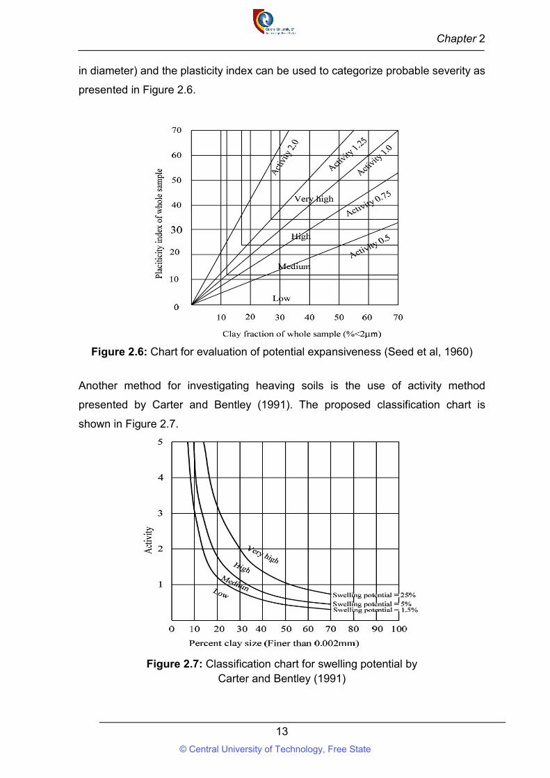
Chapter 2

13

in diameter) and the plasticity index can be used to categorize probable severity as

presented in Figure 2.6.

Figure 2.6: Chart for evaluation of potential expansiveness (Seed et al, 1960)

Another method for investigating heaving soils is the use of activity method

presented by Carter and Bentley (1991). The proposed classification chart is

shown in Figure 2.7.

Figure 2.7: Classification chart for swelling potential by Carter and Bentley (1991)


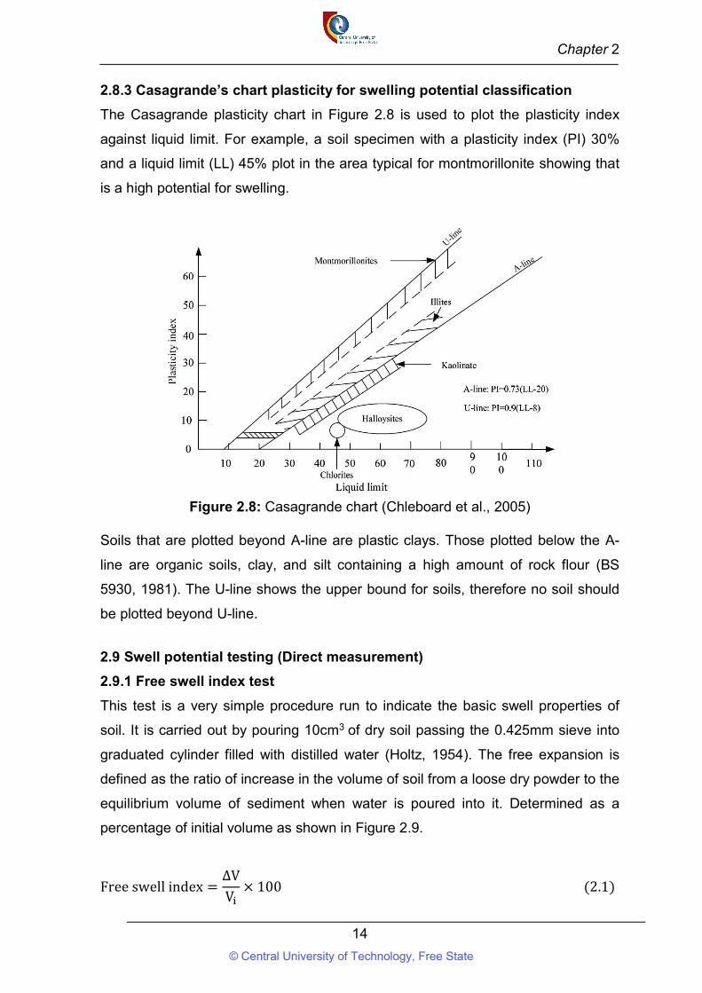
Chapter 2

14

2.8.3 Casagrande’s chart plasticity for swelling potential classification

The Casagrande plasticity chart in Figure 2.8 is used to plot the plasticity index

against liquid limit. For example, a soil specimen with a plasticity index (PI) 30%

and a liquid limit (LL) 45% plot in the area typical for montmorillonite showing that

is a high potential for swelling.

Figure 2.8: Casagrande chart (Chleboard et al., 2005)

Soils that are plotted beyond A-line are plastic clays. Those plotted below the A-

line are organic soils, clay, and silt containing a high amount of rock flour (BS

5930, 1981). The U-line shows the upper bound for soils, therefore no soil should

be plotted beyond U-line.

2.9 Swell potential testing (Direct measurement)

2.9.1 Free swell index test

This test is a very simple procedure run to indicate the basic swell properties of

soil. It is carried out by pouring 10cm3 of dry soil passing the 0.425mm sieve into

graduated cylinder filled with distilled water (Holtz, 1954). The free expansion is

defined as the ratio of increase in the volume of soil from a loose dry powder to the

equilibrium volume of sediment when water is poured into it. Determined as a

percentage of initial volume as shown in Figure 2.9.

Free swell index =∆V

V× 100 (2.1)


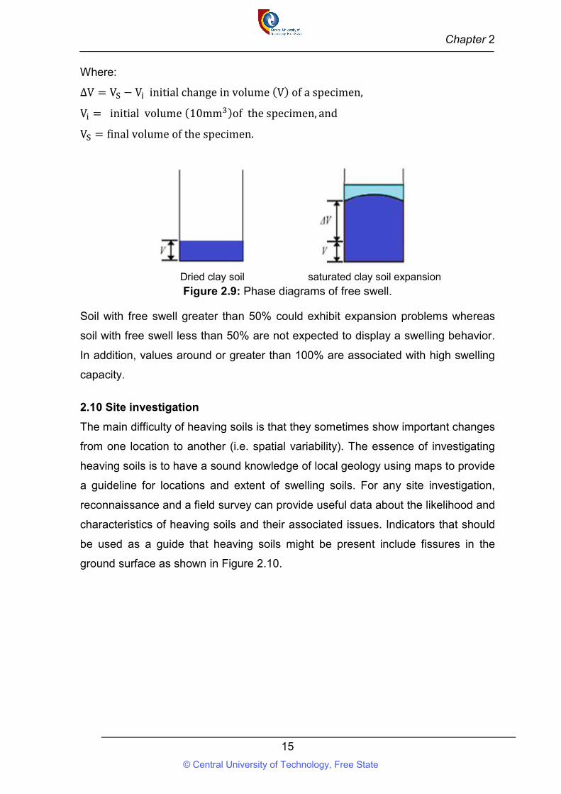
Chapter 2

15

Where:

∆V = V − V initial change in volume (V) of a specimen,

V = initial volume (10mm )of the specimen, and

V = final volume of the specimen.

Dried clay soil saturated clay soil expansion

Figure 2.9: Phase diagrams of free swell.

Soil with free swell greater than 50% could exhibit expansion problems whereas

soil with free swell less than 50% are not expected to display a swelling behavior.

In addition, values around or greater than 100% are associated with high swelling

capacity.

2.10 Site investigation

The main difficulty of heaving soils is that they sometimes show important changes

from one location to another (i.e. spatial variability). The essence of investigating

heaving soils is to have a sound knowledge of local geology using maps to provide

a guideline for locations and extent of swelling soils. For any site investigation,

reconnaissance and a field survey can provide useful data about the likelihood and

characteristics of heaving soils and their associated issues. Indicators that should

be used as a guide that heaving soils might be present include fissures in the

ground surface as shown in Figure 2.10.


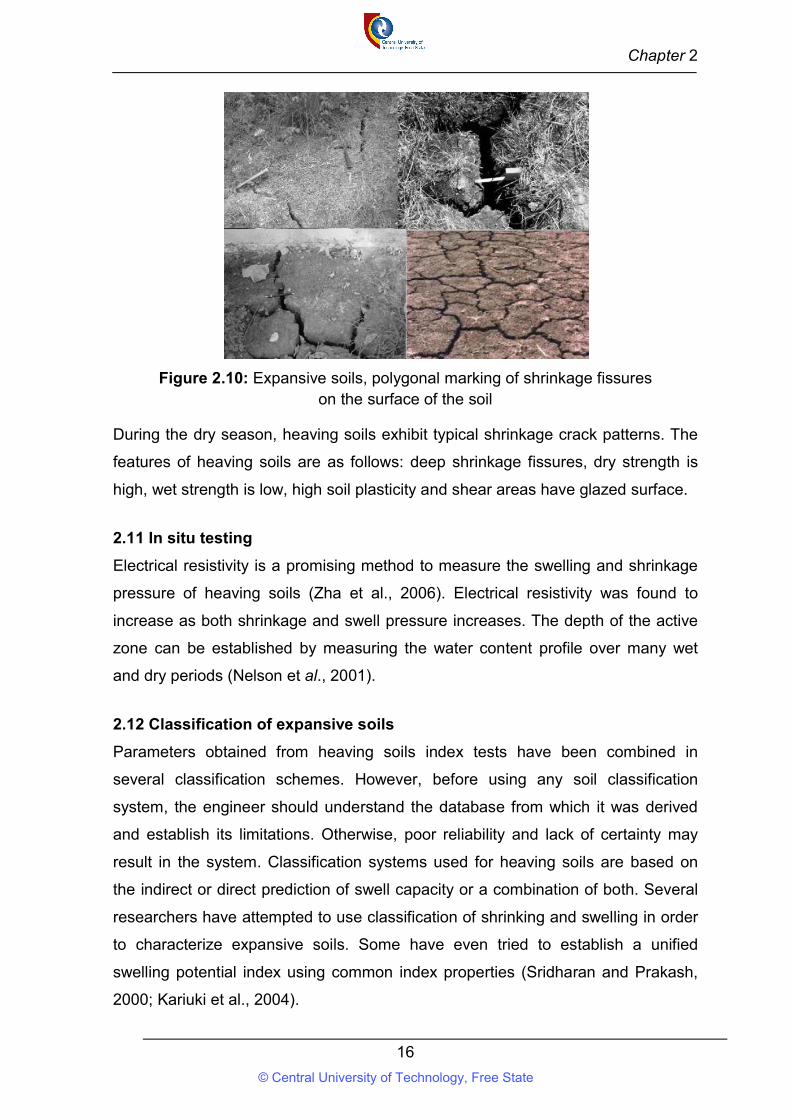
Chapter 2

16

Figure 2.10: Expansive soils, polygonal marking of shrinkage fissures on the surface of the soil

During the dry season, heaving soils exhibit typical shrinkage crack patterns. The

features of heaving soils are as follows: deep shrinkage fissures, dry strength is

high, wet strength is low, high soil plasticity and shear areas have glazed surface.

2.11 In situ testing

Electrical resistivity is a promising method to measure the swelling and shrinkage

pressure of heaving soils (Zha et al., 2006). Electrical resistivity was found to

increase as both shrinkage and swell pressure increases. The depth of the active

zone can be established by measuring the water content profile over many wet

and dry periods (Nelson et al., 2001).

2.12 Classification of expansive soils

Parameters obtained from heaving soils index tests have been combined in

several classification schemes. However, before using any soil classification

system, the engineer should understand the database from which it was derived

and establish its limitations. Otherwise, poor reliability and lack of certainty may

result in the system. Classification systems used for heaving soils are based on

the indirect or direct prediction of swell capacity or a combination of both. Several

researchers have attempted to use classification of shrinking and swelling in order

to characterize expansive soils. Some have even tried to establish a unified

swelling potential index using common index properties (Sridharan and Prakash,

2000; Kariuki et al., 2004).


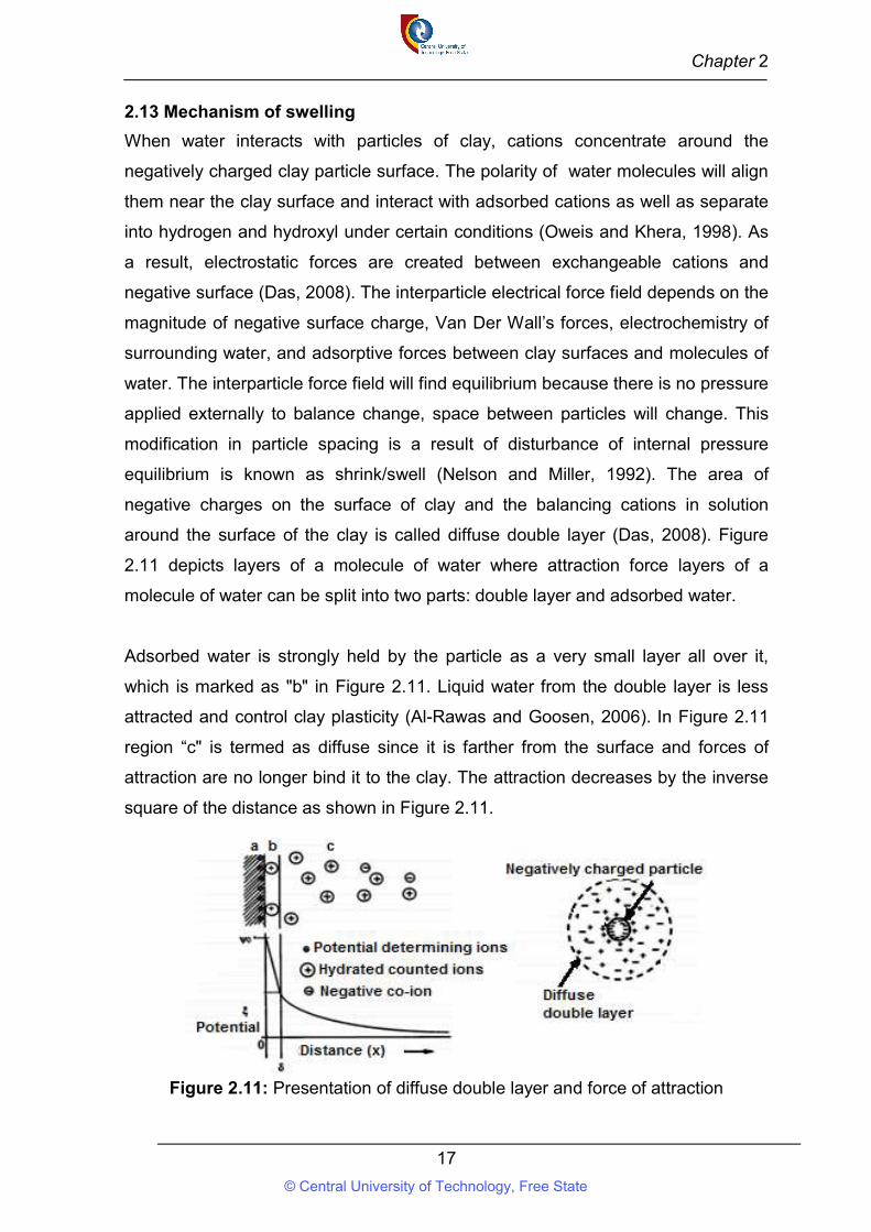
Chapter 2

17

2.13 Mechanism of swelling

When water interacts with particles of clay, cations concentrate around the

negatively charged clay particle surface. The polarity of water molecules will align

them near the clay surface and interact with adsorbed cations as well as separate

into hydrogen and hydroxyl under certain conditions (Oweis and Khera, 1998). As

a result, electrostatic forces are created between exchangeable cations and

negative surface (Das, 2008). The interparticle electrical force field depends on the

magnitude of negative surface charge, Van Der Wall’s forces, electrochemistry of

surrounding water, and adsorptive forces between clay surfaces and molecules of

water. The interparticle force field will find equilibrium because there is no pressure

applied externally to balance change, space between particles will change. This

modification in particle spacing is a result of disturbance of internal pressure

equilibrium is known as shrink/swell (Nelson and Miller, 1992). The area of

negative charges on the surface of clay and the balancing cations in solution

around the surface of the clay is called diffuse double layer (Das, 2008). Figure

2.11 depicts layers of a molecule of water where attraction force layers of a

molecule of water can be split into two parts: double layer and adsorbed water.

Adsorbed water is strongly held by the particle as a very small layer all over it,

which is marked as "b" in Figure 2.11. Liquid water from the double layer is less

attracted and control clay plasticity (Al-Rawas and Goosen, 2006). In Figure 2.11

region “c" is termed as diffuse since it is farther from the surface and forces of

attraction are no longer bind it to the clay. The attraction decreases by the inverse

square of the distance as shown in Figure 2.11.

Figure 2.11: Presentation of diffuse double layer and force of attraction


Chapter 2

18

A theoretical expression is proposed by Gouy - Chapman in Equation 2.2 for

diffuse double layer thickness: (t) which can be assumed as radius in Figure 2.11.

t =ε × k × T

8 × π × η × e × v (2.2)

The diffuse double layer thickness depends on dielectric constant medium (ε ),

Boltzmann’s constant (k), absolute temperature (T), electrolyte concentration (η),

unit electronic charge (ec) and cation valence (𝑣). Diffuse double layer thickness is

critical for the evaluation of the expansive capability and the permeability of the

soil. The interparticle spacing increases while the thickness diminishes. Therefore,

water can easily penetrate and result in an expansion of interparticle spacing.

Patel et al., (2007) stated that clays expand in two manners: hydration of surface

and osmotic expansion. Hydration of surface occurs where water molecules layer

is adsorbed on the crystal surface by hydrogen bonding. Water molecules in

successive layers increase spacing with a quasi-crystalline alignment. However,

when osmotic water moves between unit layers in clay mineral from the higher

cation concentration to lower concentrations, bulk volume increases. This process

is called osmotic expansion. The increase of volume triggered by osmotic

expansion is greater than that is generated by hydration of surface. Some clay

mineral like sodium montmorillonite undergoes osmotic expansion whereas

hydration of surface happens in all categories of clays.

2.14 Factors affecting the swell/ shrink behaviour of soil

The shrink-swell capacity of heaving soils is controlled by its initial amount of

water; void proportion; vertical pressure; internal structure, the type and amount

clay minerals in the soil. These minerals determine the normal expansion of the

soil and include smectite, montmorillonite, nontronite, vermiculite, illite, and

chlorite. For the most part, the larger the quantity of these minerals present in the

soil, the more the expansive capacity. Nonetheless, these swelling impacts may

reduce due to the presence of certain non-swelling minerals, for example,

carbonate and quartz.

Swelling stress can cause heaving, or lifting, of structures while shrinkage can

cause differential settlement. Defect results when the volume changes are


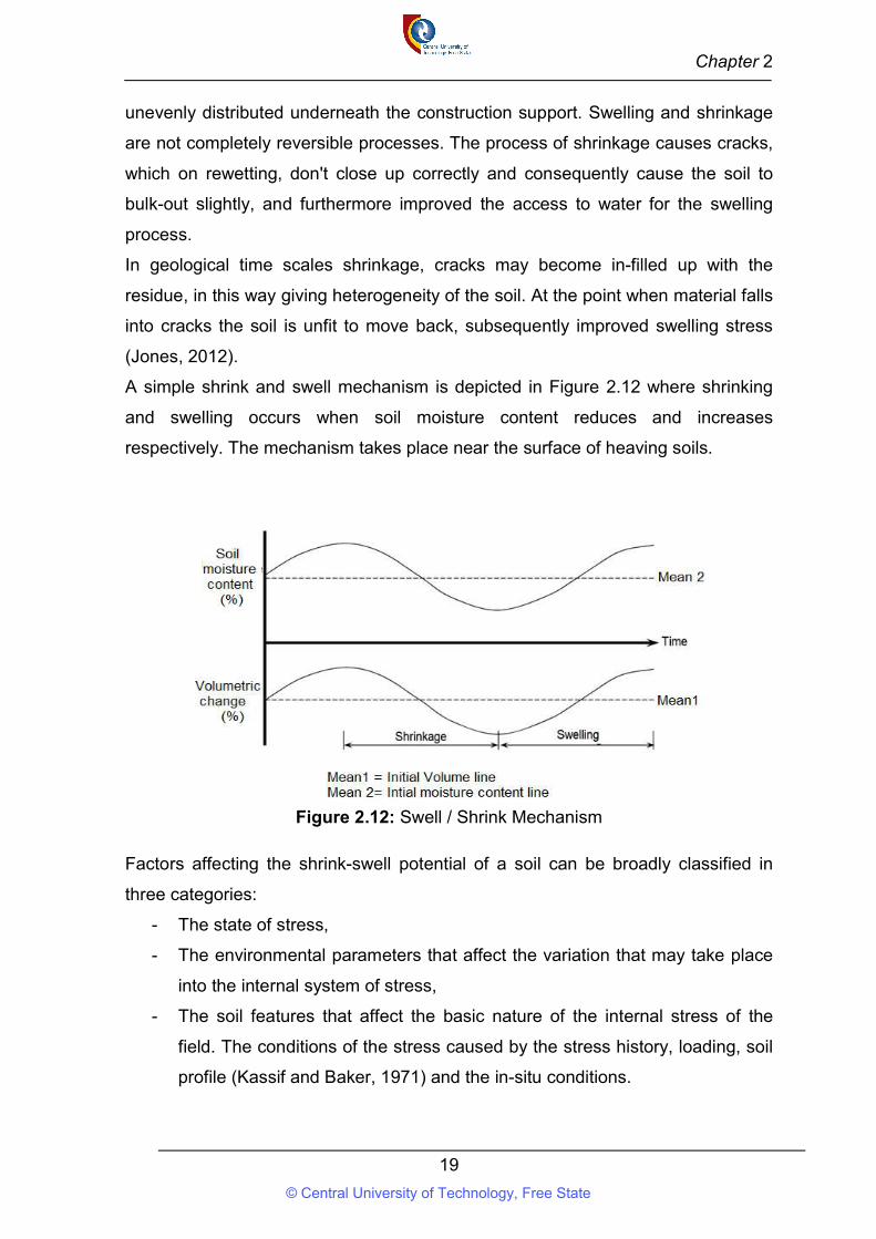
Chapter 2

19

unevenly distributed underneath the construction support. Swelling and shrinkage

are not completely reversible processes. The process of shrinkage causes cracks,

which on rewetting, don't close up correctly and consequently cause the soil to

bulk-out slightly, and furthermore improved the access to water for the swelling

process.

In geological time scales shrinkage, cracks may become in-filled up with the

residue, in this way giving heterogeneity of the soil. At the point when material falls

into cracks the soil is unfit to move back, subsequently improved swelling stress

(Jones, 2012).

A simple shrink and swell mechanism is depicted in Figure 2.12 where shrinking

and swelling occurs when soil moisture content reduces and increases

respectively. The mechanism takes place near the surface of heaving soils.

Figure 2.12: Swell / Shrink Mechanism

Factors affecting the shrink-swell potential of a soil can be broadly classified in

three categories:

- The state of stress,

- The environmental parameters that affect the variation that may take place

into the internal system of stress,

- The soil features that affect the basic nature of the internal stress of the

field. The conditions of the stress caused by the stress history, loading, soil

profile (Kassif and Baker, 1971) and the in-situ conditions.


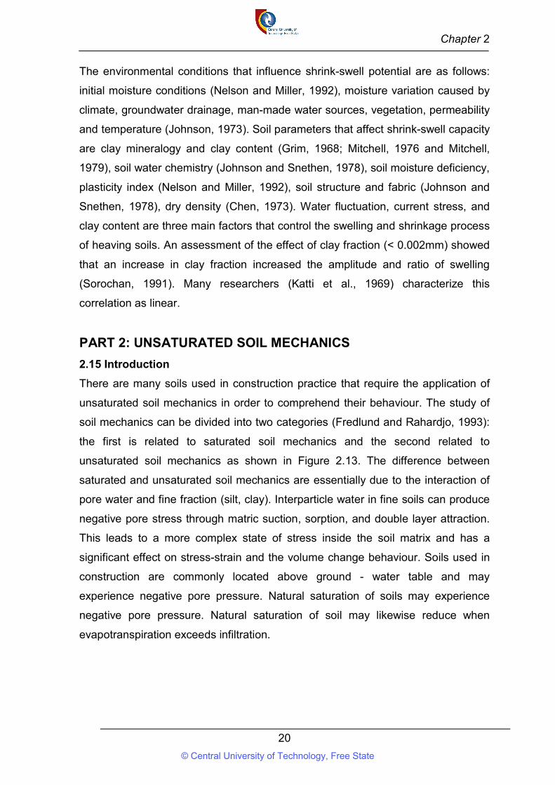
Chapter 2

20

The environmental conditions that influence shrink-swell potential are as follows:

initial moisture conditions (Nelson and Miller, 1992), moisture variation caused by

climate, groundwater drainage, man-made water sources, vegetation, permeability

and temperature (Johnson, 1973). Soil parameters that affect shrink-swell capacity

are clay mineralogy and clay content (Grim, 1968; Mitchell, 1976 and Mitchell,

1979), soil water chemistry (Johnson and Snethen, 1978), soil moisture deficiency,

plasticity index (Nelson and Miller, 1992), soil structure and fabric (Johnson and

Snethen, 1978), dry density (Chen, 1973). Water fluctuation, current stress, and

clay content are three main factors that control the swelling and shrinkage process

of heaving soils. An assessment of the effect of clay fraction (< 0.002mm) showed

that an increase in clay fraction increased the amplitude and ratio of swelling

(Sorochan, 1991). Many researchers (Katti et al., 1969) characterize this

correlation as linear.

PART 2: UNSATURATED SOIL MECHANICS

2.15 Introduction

There are many soils used in construction practice that require the application of

unsaturated soil mechanics in order to comprehend their behaviour. The study of

soil mechanics can be divided into two categories (Fredlund and Rahardjo, 1993):

the first is related to saturated soil mechanics and the second related to

unsaturated soil mechanics as shown in Figure 2.13. The difference between

saturated and unsaturated soil mechanics are essentially due to the interaction of

pore water and fine fraction (silt, clay). Interparticle water in fine soils can produce

negative pore stress through matric suction, sorption, and double layer attraction.

This leads to a more complex state of stress inside the soil matrix and has a

significant effect on stress-strain and the volume change behaviour. Soils used in

construction are commonly located above ground - water table and may

experience negative pore pressure. Natural saturation of soils may experience

negative pore pressure. Natural saturation of soil may likewise reduce when

evapotranspiration exceeds infiltration.


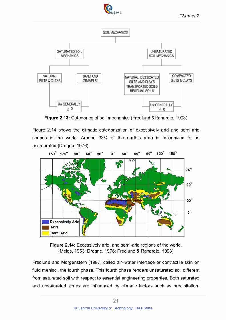
Chapter 2

21

Figure 2.13: Categories of soil mechanics (Fredlund &Rahardjo, 1993)

Figure 2.14 shows the climatic categorization of excessively arid and semi-arid

spaces in the world. Around 33% of the earth’s area is recognized to be

unsaturated (Dregne, 1976).

Figure 2.14: Excessively arid, and semi-arid regions of the world.

(Meigs, 1953; Dregne, 1976; Fredlund & Rahardjo, 1993) Fredlund and Morgenstern (1997) called air–water interface or contractile skin on

fluid menisci, the fourth phase. This fourth phase renders unsaturated soil different

from saturated soil with respect to essential engineering properties. Both saturated

and unsaturated zones are influenced by climatic factors such as precipitation,


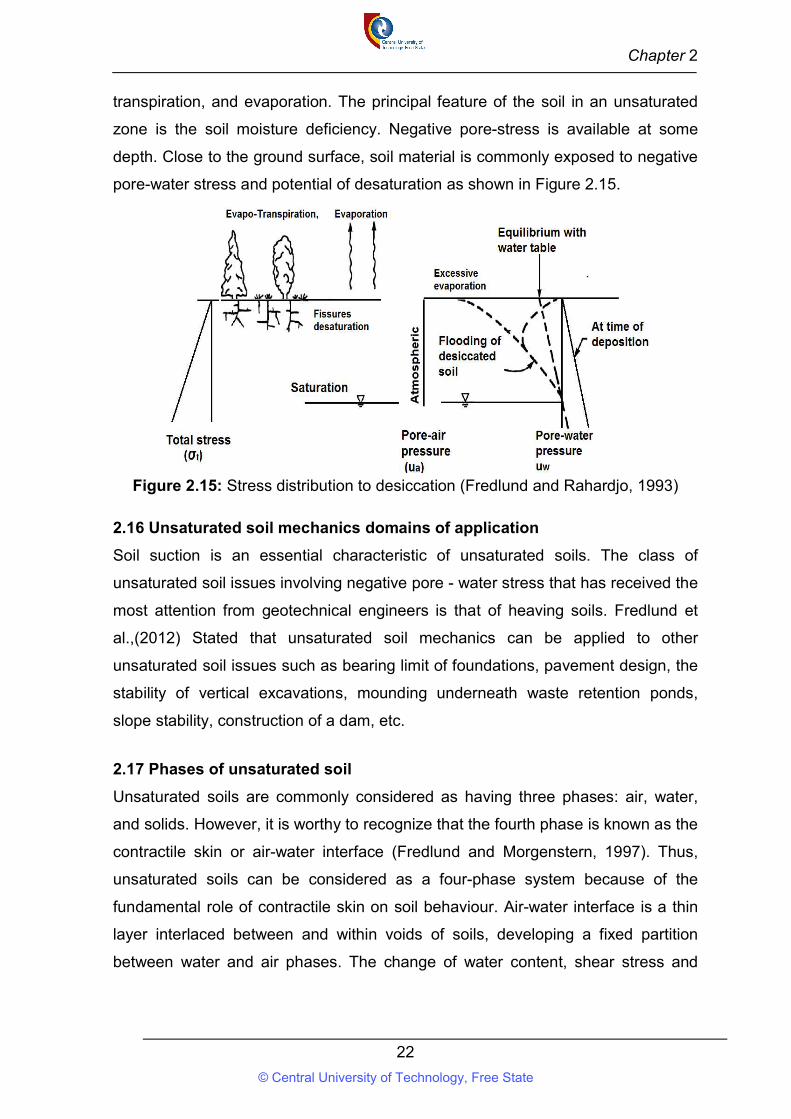
Chapter 2

22

transpiration, and evaporation. The principal feature of the soil in an unsaturated

zone is the soil moisture deficiency. Negative pore-stress is available at some

depth. Close to the ground surface, soil material is commonly exposed to negative

pore-water stress and potential of desaturation as shown in Figure 2.15.

Figure 2.15: Stress distribution to desiccation (Fredlund and Rahardjo, 1993)

2.16 Unsaturated soil mechanics domains of application

Soil suction is an essential characteristic of unsaturated soils. The class of

unsaturated soil issues involving negative pore - water stress that has received the

most attention from geotechnical engineers is that of heaving soils. Fredlund et

al.,(2012) Stated that unsaturated soil mechanics can be applied to other

unsaturated soil issues such as bearing limit of foundations, pavement design, the

stability of vertical excavations, mounding underneath waste retention ponds,

slope stability, construction of a dam, etc.

2.17 Phases of unsaturated soil

Unsaturated soils are commonly considered as having three phases: air, water,

and solids. However, it is worthy to recognize that the fourth phase is known as the

contractile skin or air-water interface (Fredlund and Morgenstern, 1997). Thus,

unsaturated soils can be considered as a four-phase system because of the

fundamental role of contractile skin on soil behaviour. Air-water interface is a thin

layer interlaced between and within voids of soils, developing a fixed partition

between water and air phases. The change of water content, shear stress and


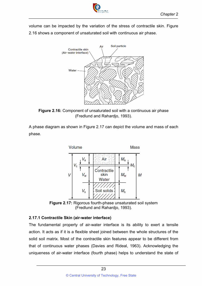
Chapter 2

23

volume can be impacted by the variation of the stress of contractile skin. Figure

2.16 shows a component of unsaturated soil with continuous air phase.

Figure 2.16: Component of unsaturated soil with a continuous air phase (Fredlund and Rahardjo, 1993).

A phase diagram as shown in Figure 2.17 can depict the volume and mass of each

phase.

Figure 2.17: Rigorous fourth-phase unsaturated soil system

(Fredlund and Rahardjo, 1993). 2.17.1 Contractile Skin (air-water interface)

The fundamental property of air-water interface is its ability to exert a tensile

action. It acts as if it is a flexible sheet joined between the whole structures of the

solid soil matrix. Most of the contractile skin features appear to be different from

that of continuous water phases (Davies and Rideal, 1963). Acknowledging the

uniqueness of air-water interface (fourth phase) helps to understand the state of


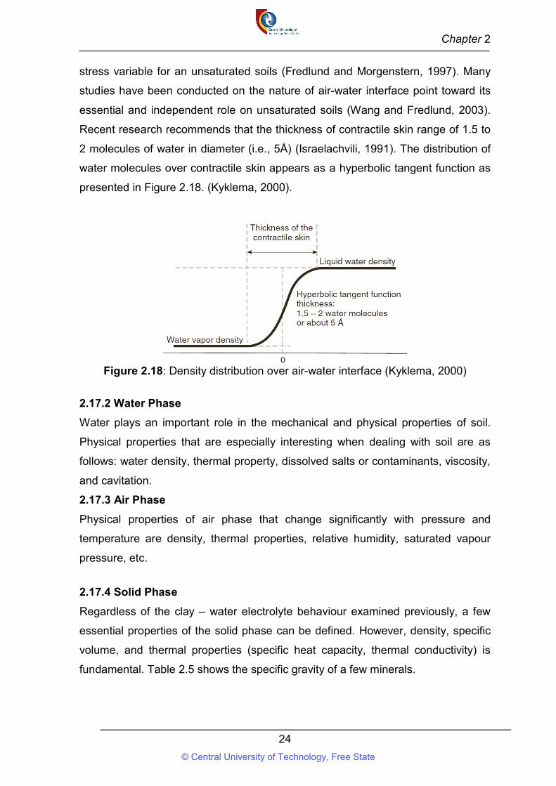
Chapter 2

24

stress variable for an unsaturated soils (Fredlund and Morgenstern, 1997). Many

studies have been conducted on the nature of air-water interface point toward its

essential and independent role on unsaturated soils (Wang and Fredlund, 2003).

Recent research recommends that the thickness of contractile skin range of 1.5 to

2 molecules of water in diameter (i.e., 5Å) (Israelachvili, 1991). The distribution of

water molecules over contractile skin appears as a hyperbolic tangent function as

presented in Figure 2.18. (Kyklema, 2000).

Figure 2.18: Density distribution over air-water interface (Kyklema, 2000)

2.17.2 Water Phase

Water plays an important role in the mechanical and physical properties of soil.

Physical properties that are especially interesting when dealing with soil are as

follows: water density, thermal property, dissolved salts or contaminants, viscosity,

and cavitation.

2.17.3 Air Phase

Physical properties of air phase that change significantly with pressure and

temperature are density, thermal properties, relative humidity, saturated vapour

pressure, etc.

2.17.4 Solid Phase

Regardless of the clay – water electrolyte behaviour examined previously, a few

essential properties of the solid phase can be defined. However, density, specific

volume, and thermal properties (specific heat capacity, thermal conductivity) is

fundamental. Table 2.5 shows the specific gravity of a few minerals.


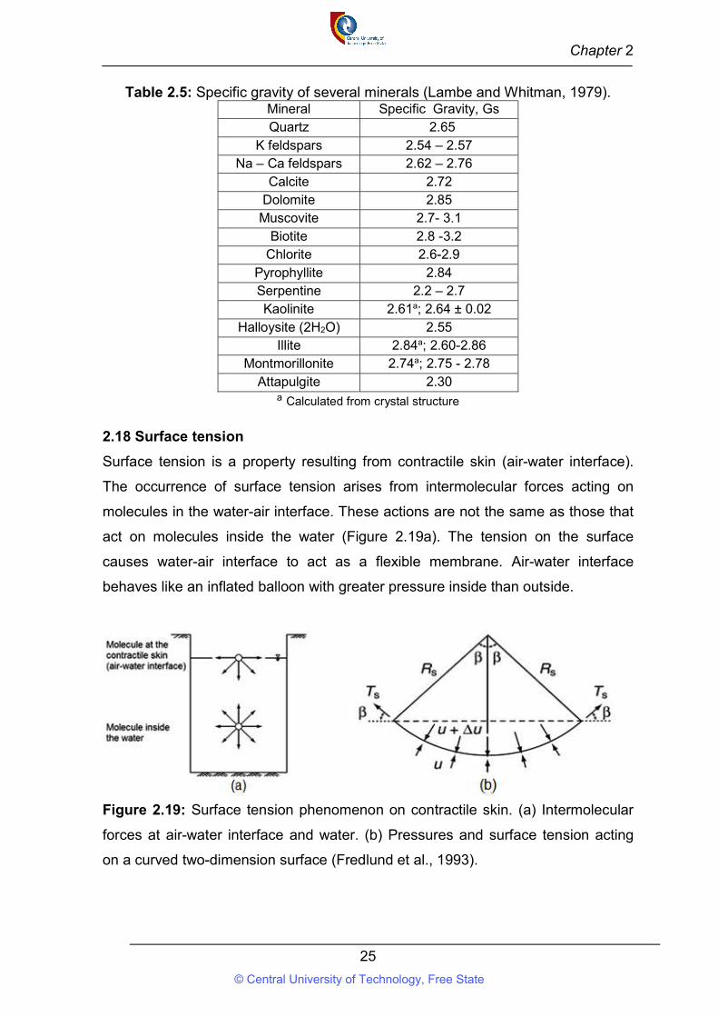
Chapter 2

25

Table 2.5: Specific gravity of several minerals (Lambe and Whitman, 1979). Mineral Specific Gravity, Gs Quartz 2.65

K feldspars 2.54 – 2.57 Na – Ca feldspars 2.62 – 2.76

Calcite 2.72 Dolomite 2.85 Muscovite 2.7- 3.1

Biotite 2.8 -3.2 Chlorite 2.6-2.9

Pyrophyllite 2.84 Serpentine 2.2 – 2.7 Kaolinite 2.61a; 2.64 ± 0.02

Halloysite (2H2O) 2.55 Illite 2.84a; 2.60-2.86

Montmorillonite 2.74a; 2.75 - 2.78 Attapulgite 2.30

a Calculated from crystal structure 2.18 Surface tension

Surface tension is a property resulting from contractile skin (air-water interface).

The occurrence of surface tension arises from intermolecular forces acting on

molecules in the water-air interface. These actions are not the same as those that

act on molecules inside the water (Figure 2.19a). The tension on the surface

causes water-air interface to act as a flexible membrane. Air-water interface

behaves like an inflated balloon with greater pressure inside than outside.

Figure 2.19: Surface tension phenomenon on contractile skin. (a) Intermolecular

forces at air-water interface and water. (b) Pressures and surface tension acting

on a curved two-dimension surface (Fredlund et al., 1993).


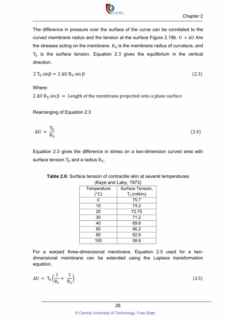
Chapter 2

26

The difference in pressure over the surface of the curve can be correlated to the

curved membrane radius and the tension at the surface Figure 2.19b. U + ∆U Are

the stresses acting on the membrane. R is the membrane radius of curvature, and

T is the surface tension. Equation 2.3 gives the equilibrium in the vertical

direction.

2 T sinβ = 2 ∆U R sin β (2.3)

Where:

2 ∆U R sin β = Length of the membrane projected onto a plane surface

Rearranging of Equation 2.3

∆U = T

R (2.4)

Equation 2.3 gives the difference in stress on a two-dimension curved area with

surface tension T and a radius R .

Table 2.6: Surface tension of contractile skin at several temperatures (Kaye and Laby, 1973)

Temperature (°C)

Surface Tension, Ts (mN/m)

0 75.7 10 74.2 20 72.75 30 71.2 40 69.6 60 66.2 80 62.6

100 58.8

For a warped three-dimensional membrane, Equation 2.5 used for a two-dimensional membrane can be extended using the Laplace transformation equation.

∆U = T1

R+

1

R (2.5)


Chapter 2

27

Where: R , R = Radii of curvature of a warped membrane according to the orthogonal

principal planes

Figure 2.20: Surface tension on the three-dimension warped membrane

(Fredlund and Rahardjo, 1993)

In unsaturated soil, air-water interface is governed by pore water pressure uw

smaller than pore air pressure ua. The stress difference (ua - uw) is referred to as

matric suction. Equation 2.6 gives the difference in stress created by the

contractile layer to bend to a curvature. Equation 2.6 is referred to as Kelvin’s

capillary model equation.

U − U = 2T

R (2.6)

2.19 Capillary phenomenon

Matric suction component of the total suction drives capillary transport. The level of

water rise inside a capillary tube and the radius of curvature of meniscus directly

affects the matric suction. The curvature of the meniscus is related to water

content since various portions of particle-matrix hold the menisci as saturation

changes. Generally, at lower saturation, the menisci are smaller (higher tension)

and higher saturations have larger menisci (lower tension). This relationship is


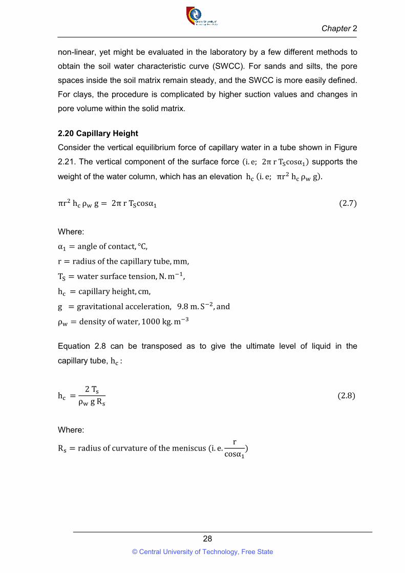
Chapter 2

28

non-linear, yet might be evaluated in the laboratory by a few different methods to

obtain the soil water characteristic curve (SWCC). For sands and silts, the pore

spaces inside the soil matrix remain steady, and the SWCC is more easily defined.

For clays, the procedure is complicated by higher suction values and changes in

pore volume within the solid matrix.

2.20 Capillary Height

Consider the vertical equilibrium force of capillary water in a tube shown in Figure

2.21. The vertical component of the surface force (i. e; 2π r T cosα ) supports the

weight of the water column, which has an elevation h (i. e; πr h ρ g).

πr h ρ g = 2π r T cosα (2.7)

Where:

α = angle of contact, °C,

r = radius of the capillary tube, mm,

T = water surface tension, N. m ,

h = capillary height, cm,

g = gravitational acceleration, 9.8 m. S , and

ρ = density of water, 1000 kg. m

Equation 2.8 can be transposed as to give the ultimate level of liquid in the

capillary tube, h :

h =2 T

ρ g R (2.8)

Where:

R = radius of curvature of the meniscus (i. e.r

cosα)


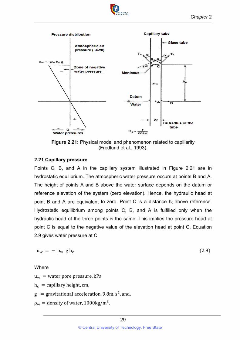
Chapter 2

29

Figure 2.21: Physical model and phenomenon related to capillarity (Fredlund et al., 1993).

2.21 Capillary pressure

Points C, B, and A in the capillary system illustrated in Figure 2.21 are in

hydrostatic equilibrium. The atmospheric water pressure occurs at points B and A.

The height of points A and B above the water surface depends on the datum or

reference elevation of the system (zero elevation). Hence, the hydraulic head at

point B and A are equivalent to zero. Point C is a distance hc above reference.

Hydrostatic equilibrium among points C, B, and A is fulfilled only when the

hydraulic head of the three points is the same. This implies the pressure head at

point C is equal to the negative value of the elevation head at point C. Equation

2.9 gives water pressure at C.

u = − ρ g h (2.9)

Where

u = water pore pressure, kPa

h = capillary height, cm,

g = gravitational acceleration, 9.8m. s , and,

ρ = density of water, 1000kg/m .


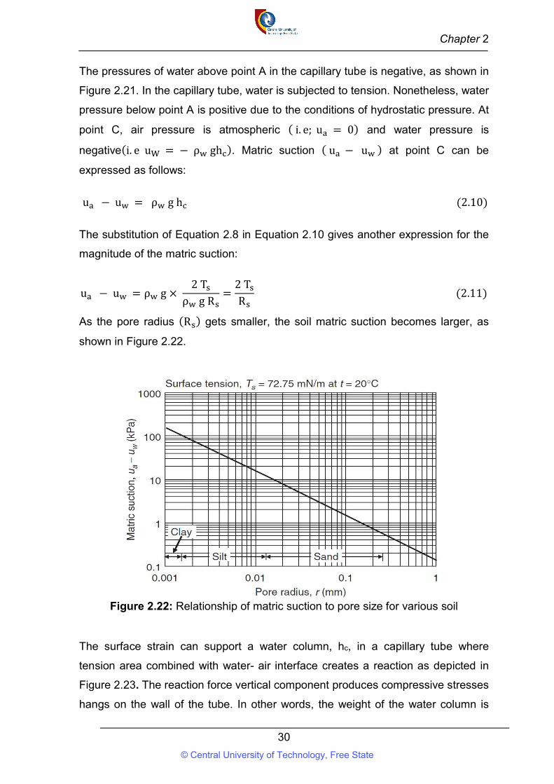
Chapter 2

30

The pressures of water above point A in the capillary tube is negative, as shown in

Figure 2.21. In the capillary tube, water is subjected to tension. Nonetheless, water

pressure below point A is positive due to the conditions of hydrostatic pressure. At

point C, air pressure is atmospheric ( i. e; u = 0) and water pressure is

negative(i. e u = − ρ gh ). Matric suction ( u − u ) at point C can be

expressed as follows:

u − u = ρ g h (2.10)

The substitution of Equation 2.8 in Equation 2.10 gives another expression for the

magnitude of the matric suction:

u − u = ρ g × 2 T

ρ g R=

2 T

R (2.11)

As the pore radius (R ) gets smaller, the soil matric suction becomes larger, as


Figure 2.22: Relationship of matric suction to pore size for various soil

The surface strain can support a water column, hc, in a capillary tube where

tension area combined with water- air interface creates a reaction as depicted in

Figure 2.23. The reaction force vertical component produces compressive stresses

hangs on the wall of the tube. In other words, the weight of the water column is


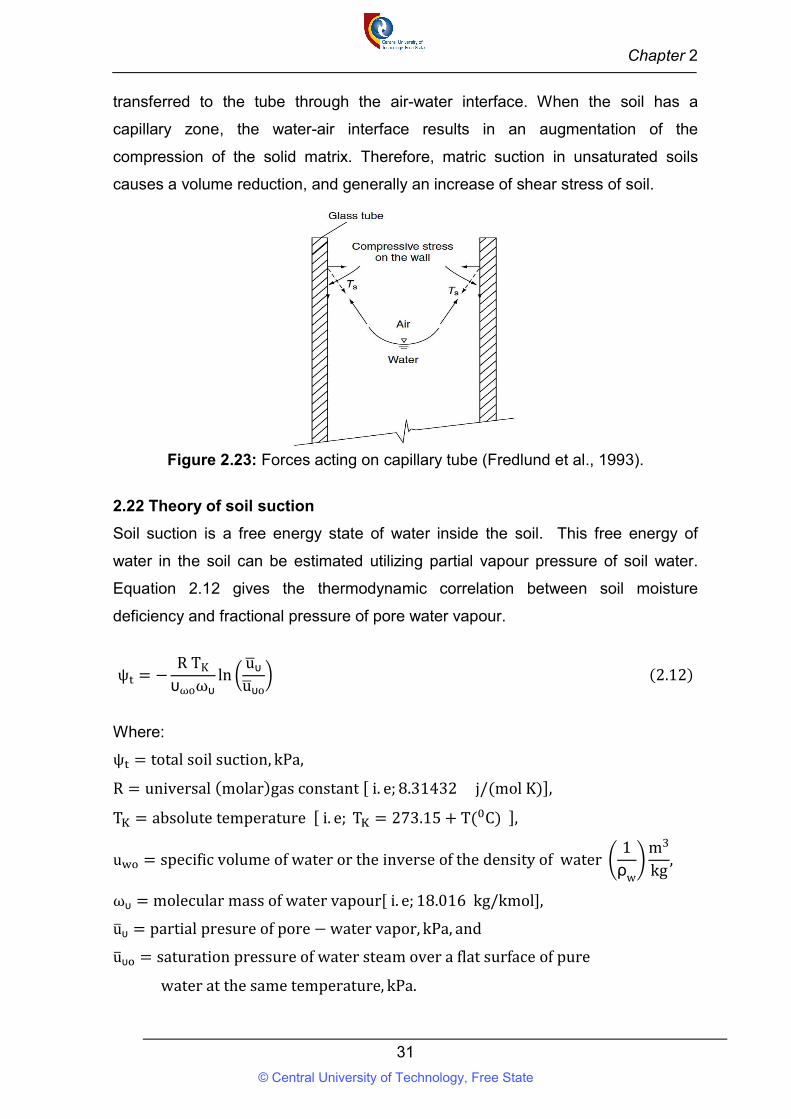
Chapter 2

31

transferred to the tube through the air-water interface. When the soil has a

capillary zone, the water-air interface results in an augmentation of the

compression of the solid matrix. Therefore, matric suction in unsaturated soils

causes a volume reduction, and generally an increase of shear stress of soil.

Figure 2.23: Forces acting on capillary tube (Fredlund et al., 1993).

2.22 Theory of soil suction

Soil suction is a free energy state of water inside the soil. This free energy of

water in the soil can be estimated utilizing partial vapour pressure of soil water.

Equation 2.12 gives the thermodynamic correlation between soil moisture

deficiency and fractional pressure of pore water vapour.

ψ = −R TK

υωoωυln

uυ

uυo (2.12)

Where:

ψ = total soil suction, kPa,

R = universal (molar)gas constant [ i. e; 8.31432 j/(mol K)],

T = absolute temperature [ i. e; T = 273.15 + T( C) ],

u = specific volume of water or the inverse of the density of water 1

ρw

m3

kg,

ωυ = molecular mass of water vapour[ i. e; 18.016 kg/kmol],

uυ = partial presure of pore − water vapor, kPa, and

uυ = saturation pressure of water steam over a flat surface of pure

water at the same temperature, kPa.


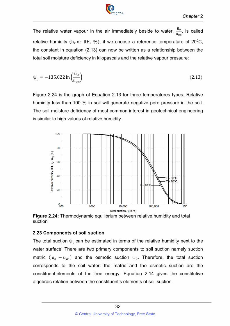
Chapter 2

32

The relative water vapour in the air immediately beside to water, υ

υ, is called

relative humidity (h or RH, %), if we choose a reference temperature of 200C,

the constant in equation (2.13) can now be written as a relationship between the

total soil moisture deficiency in kilopascals and the relative vapour pressure:

ψ = −135,022 lnuυ

uυ (2.13)

Figure 2.24 is the graph of Equation 2.13 for three temperatures types. Relative

humidity less than 100 % in soil will generate negative pore pressure in the soil.

The soil moisture deficiency of most common interest in geotechnical engineering

is similar to high values of relative humidity.

Figure 2.24: Thermodynamic equilibrium between relative humidity and total suction 2.23 Components of soil suction

The total suction ψ can be estimated in terms of the relative humidity next to the

water surface. There are two primary components to soil suction namely suction

matric ( u − u ) and the osmotic suction ψ . Therefore, the total suction

corresponds to the soil water: the matric and the osmotic suction are the

constituent elements of the free energy. Equation 2.14 gives the constitutive

algebraic relation between the constituent’s elements of soil suction.


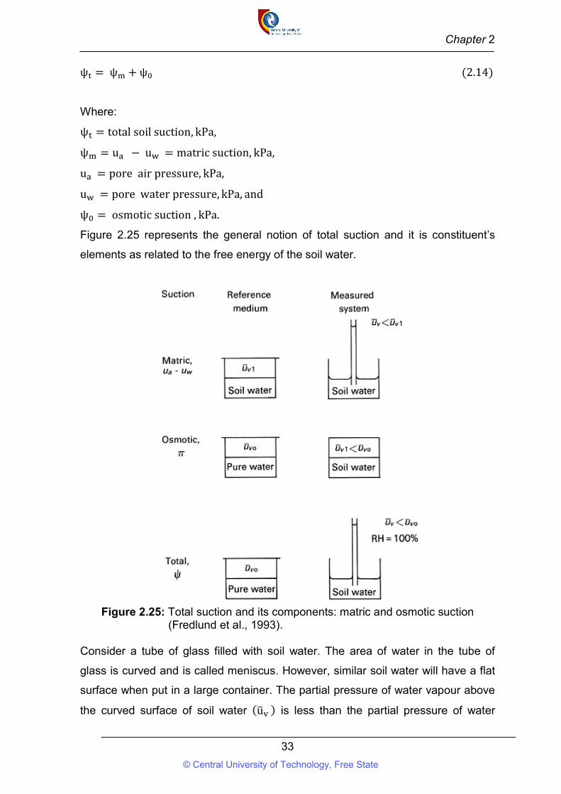
Chapter 2

33

ψ = ψ + ψ (2.14)

Where:

ψ = total soil suction, kPa,

ψ = u − u = matric suction, kPa,

u = pore air pressure, kPa,

u = pore water pressure, kPa, and

ψ = osmotic suction , kPa.

Figure 2.25 represents the general notion of total suction and it is constituent’s

elements as related to the free energy of the soil water.

Figure 2.25: Total suction and its components: matric and osmotic suction

(Fredlund et al., 1993). Consider a tube of glass filled with soil water. The area of water in the tube of

glass is curved and is called meniscus. However, similar soil water will have a flat

surface when put in a large container. The partial pressure of water vapour above

the curved surface of soil water (u ) is less than the partial pressure of water


Chapter 2

34

vapour above a plane surface of identical soil water (u ). In other words, RH in

the soil will diminish because of the curved water surfaces produced by the

capillary phenomenon. The water vapour pressure or RH diminishes as the radius

of curvature of the water surface decreases. Accordingly, the radius of curvature is

inversely proportional to the difference between the air and water pressures across

the surface ( i. e; u − u ) and is called matric suction. Consequently, one

component of the total suction is matric suction, and it contributes to a reduction in

the relative humidity.

2.24 Unsaturated soil stress state variables

As indicated by soil mechanics, the behaviour of soil relies on the stress variables

that control the equilibrium of soil material. Along these lines, the stress variable

necessary to describe the equilibrium of the soil structure can be considered as

the stress state variables for the soil. The stress variables must be quantifiable, for

example, the total stress , σ, the air-water pressure, u , and water pore

pressure, u . Stress equilibrium can be assessed on unsaturated soil, by

considering the state of stress at a point in the soil.

2.24.1 Equilibrium analysis

Body forces and surface forces can both act on an element of soil. The stress

component perpendicular to a plane is the normal stress , σ, while the parallel

component is identified as shear stress, τ. A cubical element that is completely

enclosed by imaginary, boundaries yields a free body for stress equilibrium

analysis. Figure 2.26 shows a soil element with dimensions of d , d and d in

Cartesian coordinates. The shear and normal stress on each plane of the element

are shown in Figure 2.26.


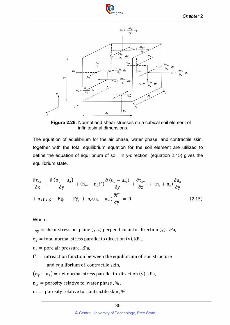
Chapter 2

35

Figure 2.26: Normal and shear stresses on a cubical soil element of infinitesimal dimensions. The equation of equilibrium for the air phase, water phase, and contractile skin,

together with the total equilibrium equation for the soil element are utilized to

define the equation of equilibrium of soil. In y-direction, (equation 2.15) gives the

equilibrium state.

∂τ

∂x +

∂ σ − u

∂y + (n + n f ∗)

∂ (u − u )

∂y +

∂τ

∂z + (n + n )

∂u

∂y

+ n ρ g − F − F + n (u − u )∂f ∗

∂y = 0 (2.15)

Where:

τ = shear stress on plane (y, z) perpendicular to direction (y), kPa,

σ = total normal stress parallel to direction (y), kPa,

u = pore air pressure, kPa,

f ∗ = intreaction function between the equilibrium of soil structure

and equilibrium of contractile skin,

σ − u = net normal stress parallel to direction (y), kPa,

n = porosity relative to water phase , % ,

n = porosity relative to contractile skin , % ,


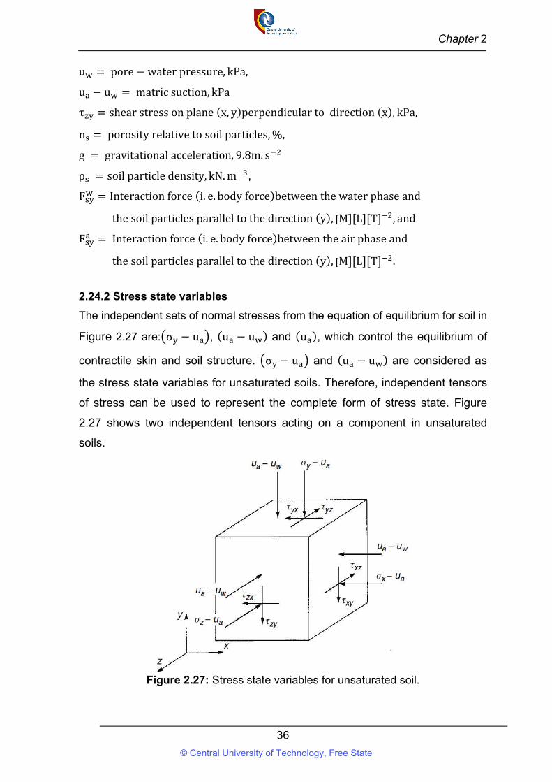
Chapter 2

36

u = pore − water pressure, kPa,

u − u = matric suction, kPa

τ = shear stress on plane (x, y)perpendicular to direction (x), kPa,

n = porosity relative to soil particles, %,

g = gravitational acceleration, 9.8m. s

ρ = soil particle density, kN. m ,

F = Interaction force (i. e. body force)between the water phase and

the soil particles parallel to the direction (y), [M][L][T] , and

F = Interaction force (i. e. body force)between the air phase and

the soil particles parallel to the direction (y), [M][L][T] .

2.24.2 Stress state variables

The independent sets of normal stresses from the equation of equilibrium for soil in

Figure 2.27 are: σ − u , (u − u ) and (u ), which control the equilibrium of

contractile skin and soil structure. σ − u and (u − u ) are considered as

the stress state variables for unsaturated soils. Therefore, independent tensors

of stress can be used to represent the complete form of stress state. Figure

2.27 shows two independent tensors acting on a component in unsaturated

soils.

Figure 2.27: Stress state variables for unsaturated soil.


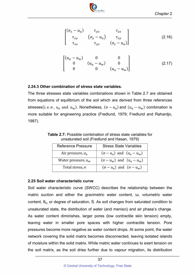
Chapter 2

37

(𝜎 − 𝑢 ) 𝜏 𝜏

𝜏 𝜎 − 𝑢 𝜏

𝜏 𝜏 (𝜎 − 𝑢 )

(2.16)

(𝑢 − 𝑢 ) 0 0

0 (𝑢 − 𝑢 ) 0

0 0 (𝑢 − 𝑢 ) (2.17)

2.24.3 Other combination of stress state variables.

The three stresses state variables combinations shown in Table 2.7 are obtained

from equations of equilibrium of the soil which are derived from three references

stresses(i. e. σ , u and u ). Nonetheless, (σ − u ) and (u − u ) combination is

more suitable for engineering practice (Fredlund, 1979; Fredlund and Rahardjo,

1987).

Table 2.7: Possible combination of stress state variables for unsaturated soil (Fredlund and Hasan, 1979)

Reference Pressure Stress State Variables

Air pressure, u (σ − u ) and (u − u )

Water pressure, u (σ − u ) and (u − u )

Total stress, σ (σ − u ) and (σ − u )

2.25 Soil water characteristic curve

Soil water characteristic curve (SWCC) describes the relationship between the

matric suction and either the gravimetric water content, ω, volumetric water

content, θs, or degree of saturation, S. As soil changes from saturated condition to

unsaturated state, the distribution of water (and menisci) and air phase’s change.

As water content diminishes, larger pores (low contractile skin tension) empty,

leaving water in smaller pore spaces with higher contractile tension. Pore

pressures become more negative as water content drops. At some point, the water

network covering the solid matrix becomes disconnected, leaving isolated islands

of moisture within the solid matrix. While matric water continues to exert tension on

the soil matrix, as the soil dries further due to vapour migration, its distribution


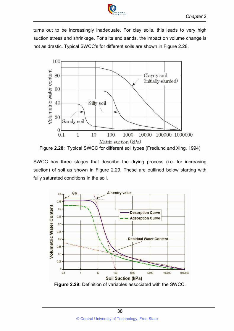
Chapter 2

38

turns out to be increasingly inadequate. For clay soils, this leads to very high

suction stress and shrinkage. For silts and sands, the impact on volume change is

not as drastic. Typical SWCC’s for different soils are shown in Figure 2.28.

Figure 2.28: Typical SWCC for different soil types (Fredlund and Xing, 1994)

SWCC has three stages that describe the drying process (i.e. for increasing

suction) of soil as shown in Figure 2.29. These are outlined below starting with

fully saturated conditions in the soil.

Figure 2.29: Definition of variables associated with the SWCC.


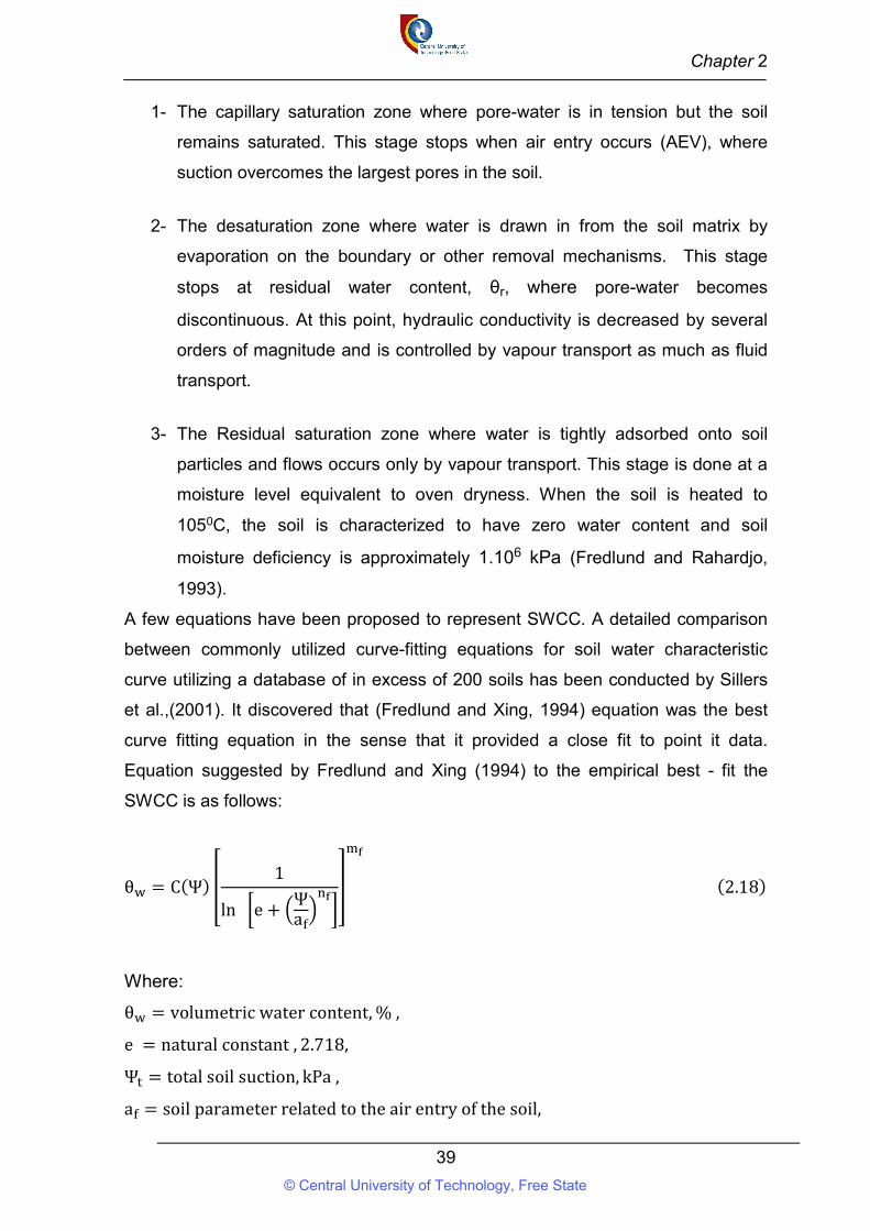
Chapter 2

39

1- The capillary saturation zone where pore-water is in tension but the soil

remains saturated. This stage stops when air entry occurs (AEV), where

suction overcomes the largest pores in the soil.

2- The desaturation zone where water is drawn in from the soil matrix by

evaporation on the boundary or other removal mechanisms. This stage

stops at residual water content, θr, where pore-water becomes

discontinuous. At this point, hydraulic conductivity is decreased by several

orders of magnitude and is controlled by vapour transport as much as fluid

transport.

3- The Residual saturation zone where water is tightly adsorbed onto soil

particles and flows occurs only by vapour transport. This stage is done at a

moisture level equivalent to oven dryness. When the soil is heated to

1050C, the soil is characterized to have zero water content and soil

moisture deficiency is approximately 1.106 kPa (Fredlund and Rahardjo,

1993).

A few equations have been proposed to represent SWCC. A detailed comparison

between commonly utilized curve-fitting equations for soil water characteristic

curve utilizing a database of in excess of 200 soils has been conducted by Sillers

et al.,(2001). It discovered that (Fredlund and Xing, 1994) equation was the best

curve fitting equation in the sense that it provided a close fit to point it data.

Equation suggested by Fredlund and Xing (1994) to the empirical best - fit the

SWCC is as follows:

θ = C(Ψ)1

ln e +Ψa

(2.18)

Where:

θ = volumetric water content, % ,

e = natural constant , 2.718,

Ψ = total soil suction, kPa ,

a = soil parameter related to the air entry of the soil,


Chapter 2

40

n = soil parameter related to the rate of desaturation,

m = soil parameter related to the residual water content conditions, and

C(Ψ) = correction factor to ensure that the function goes 10 kpa (P = 7),

of suction zero water content ; kpa = 10 .

While it is very simple to quantify the SWCC in vivo, it is still generally costly. Thus,

the assessment of the SWCC utilizing grain size analysis and volume-mass

properties is advantageous. An empirical curve could be fitted based on grain size

distribution (Fredlund, 2000).


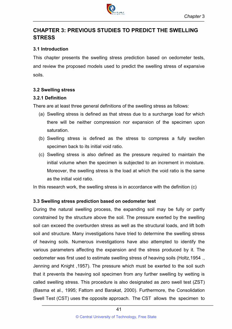
Chapter 3

41

CHAPTER 3: PREVIOUS STUDIES TO PREDICT THE SWELLING STRESS

3.1 Introduction

This chapter presents the swelling stress prediction based on oedometer tests,

and review the proposed models used to predict the swelling stress of expansive

soils.

3.2 Swelling stress

3.2.1 Definition

There are at least three general definitions of the swelling stress as follows:

(a) Swelling stress is defined as that stress due to a surcharge load for which

there will be neither compression nor expansion of the specimen upon

saturation.

(b) Swelling stress is defined as the stress to compress a fully swollen

specimen back to its initial void ratio.

(c) Swelling stress is also defined as the pressure required to maintain the

initial volume when the specimen is subjected to an increment in moisture.

Moreover, the swelling stress is the load at which the void ratio is the same

as the initial void ratio.

In this research work, the swelling stress is in accordance with the definition (c)

3.3 Swelling stress prediction based on oedometer test

During the natural swelling process, the expanding soil may be fully or partly

constrained by the structure above the soil. The pressure exerted by the swelling

soil can exceed the overburden stress as well as the structural loads, and lift both

soil and structure. Many investigations have tried to determine the swelling stress

of heaving soils. Numerous investigations have also attempted to identify the

various parameters affecting the expansion and the stress produced by it. The

oedometer was first used to estimate swelling stress of heaving soils (Holtz,1954 .,

Jenning and Knight ,1957). The pressure which must be exerted to the soil such

that it prevents the heaving soil specimen from any further swelling by wetting is

called swelling stress. This procedure is also designated as zero swell test (ZST)

(Basma et al., 1995; Fattom and Barakat, 2000). Furthermore, the Consolidation

Swell Test (CST) uses the opposite approach. The CST allows the specimen to


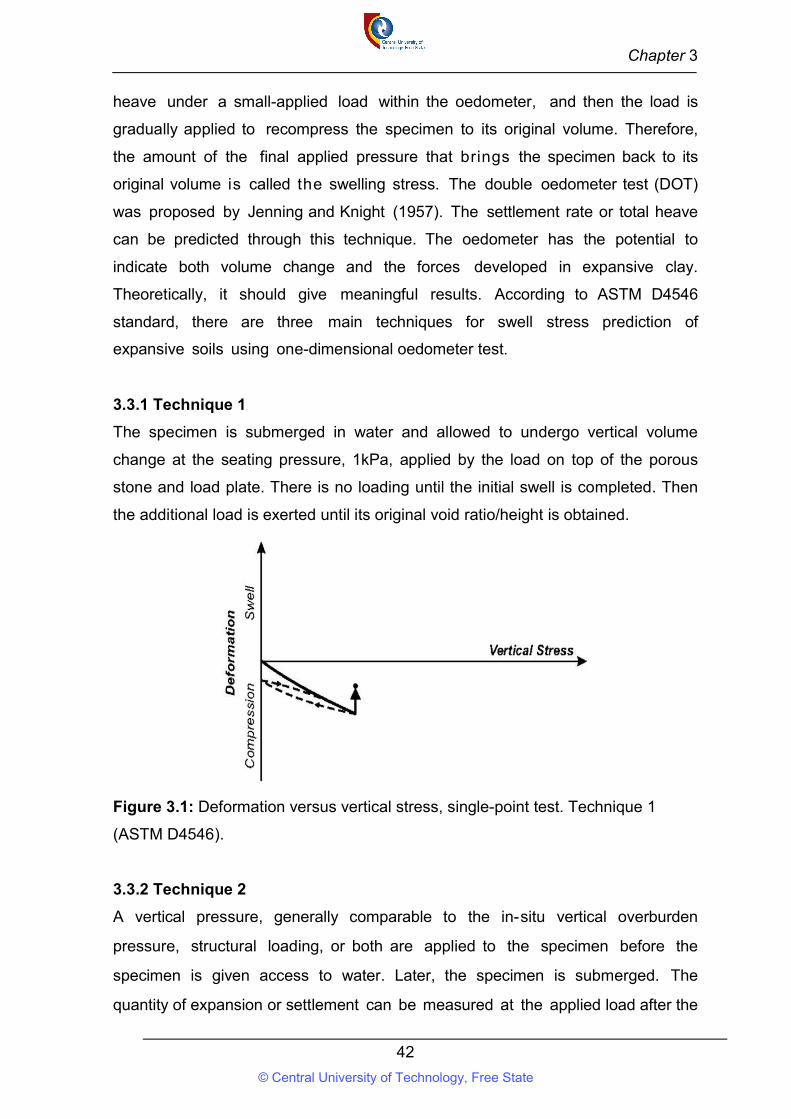
Chapter 3

42

heave under a small-applied load within the oedometer, and then the load is

gradually applied to recompress the specimen to its original volume. Therefore,

the amount of the final applied pressure that brings the specimen back to its

original volume is called the swelling stress. The double oedometer test (DOT)

was proposed by Jenning and Knight (1957). The settlement rate or total heave

can be predicted through this technique. The oedometer has the potential to

indicate both volume change and the forces developed in expansive clay.

Theoretically, it should give meaningful results. According to ASTM D4546

standard, there are three main techniques for swell stress prediction of

expansive soils using one-dimensional oedometer test.

3.3.1 Technique 1

The specimen is submerged in water and allowed to undergo vertical volume

change at the seating pressure, 1kPa, applied by the load on top of the porous

stone and load plate. There is no loading until the initial swell is completed. Then

the additional load is exerted until its original void ratio/height is obtained.

Figure 3.1: Deformation versus vertical stress, single-point test. Technique 1

(ASTM D4546).

3.3.2 Technique 2

A vertical pressure, generally comparable to the in-situ vertical overburden

pressure, structural loading, or both are applied to the specimen before the

specimen is given access to water. Later, the specimen is submerged. The

quantity of expansion or settlement can be measured at the applied load after the


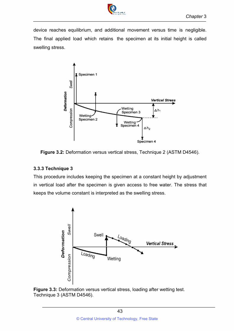
Chapter 3

43

device reaches equilibrium, and additional movement versus time is negligible.

The final applied load which retains the specimen at its initial height is called

swelling stress.

Figure 3.2: Deformation versus vertical stress, Technique 2 (ASTM D4546).

3.3.3 Technique 3

This procedure includes keeping the specimen at a constant height by adjustment

in vertical load after the specimen is given access to free water. The stress that

keeps the volume constant is interpreted as the swelling stress.

Figure 3.3: Deformation versus vertical stress, loading after wetting test. Technique 3 (ASTM D4546).


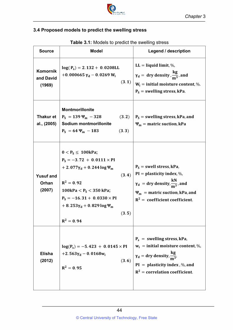
Chapter 3

44

3.4 Proposed models to predict the swelling stress

Table 3.1: Models to predict the swelling stress

Source Model Legend / description

Komornik

and David

(1969)

𝐥𝐨𝐠 ( 𝐏𝐬) = 𝟐. 𝟏𝟑𝟐 + 𝟎. 𝟎𝟐𝟎𝟖𝐋𝐋

+𝟎. 𝟎𝟎𝟎𝟔𝟔𝟓 𝛄𝐝 − 𝟎. 𝟎𝟐𝟔𝟗 𝐖𝐢

(𝟑. 𝟏)

𝐋𝐋 = 𝐥𝐢𝐪𝐮𝐢𝐝 𝐥𝐢𝐦𝐢𝐭, %,

𝛄𝐝 = 𝐝𝐫𝐲 𝐝𝐞𝐧𝐬𝐢𝐭𝐲 ,𝐤𝐠

𝐦𝟑, 𝐚𝐧𝐝

𝐖𝐢 = 𝐢𝐧𝐢𝐭𝐢𝐚𝐥 𝐦𝐨𝐢𝐬𝐭𝐮𝐫𝐞 𝐜𝐨𝐧𝐭𝐞𝐧𝐭, %.

𝐏𝐒 = 𝐬𝐰𝐞𝐥𝐥𝐢𝐧𝐠 𝐬𝐭𝐫𝐞𝐬𝐬, 𝐤𝐏𝐚.

Thakur et

al., (2005)

Montmorillonite

𝐏𝐒 = 𝟏𝟑𝟗 𝚿𝐦 − 𝟑𝟐𝟖 (𝟑. 𝟐)

Sodium montmorillonite

𝐏𝐒 = 𝟔𝟒 𝚿𝐦 − 𝟏𝟖𝟑 (𝟑. 𝟑)

𝐏𝐒 = 𝐬𝐰𝐞𝐥𝐥𝐢𝐧𝐠 𝐬𝐭𝐫𝐞𝐬𝐬, 𝐤𝐏𝐚, 𝐚𝐧𝐝

𝚿𝐦 = 𝐦𝐚𝐭𝐫𝐢𝐜 𝐬𝐮𝐜𝐭𝐢𝐨𝐧, 𝐤𝐏𝐚

Yusuf and

Orhan

(2007)

𝟎 < 𝐏𝐒 ≤ 𝟏𝟎𝟎𝐤𝐏𝐚;

𝐏𝐒 = −𝟑. 𝟕𝟐 + 𝟎. 𝟎𝟏𝟏𝟏 × 𝐏𝐈

+ 𝟐. 𝟎𝟕𝟕𝛄𝐝 + 𝟎. 𝟐𝟒𝟒 𝐥𝐨𝐠 𝚿𝐦

(𝟑. 𝟒)

𝐑𝟐 = 𝟎. 𝟗𝟐

𝟏𝟎𝟎𝐤𝐏𝐚 < 𝐏𝐒 < 𝟑𝟓𝟎 𝐤𝐏𝐚;

𝐏𝐒 = −𝟏𝟔. 𝟑𝟏 + 𝟎. 𝟎𝟑𝟑𝟎 × 𝐏𝐈

+ 𝟖. 𝟐𝟓𝟑𝛄𝐝 + 𝟎. 𝟖𝟐𝟗 𝐥𝐨𝐠 𝚿𝐦

(𝟑. 𝟓)

𝐑𝟐 = 𝟎. 𝟗𝟒

𝐏𝐒 = 𝐬𝐰𝐞𝐥𝐥 𝐬𝐭𝐫𝐞𝐬𝐬, 𝐤𝐏𝐚,

𝐏𝐈 = 𝐩𝐥𝐚𝐬𝐭𝐢𝐜𝐢𝐭𝐲 𝐢𝐧𝐝𝐞𝐱, %,

𝛄𝐝 = 𝐝𝐫𝐲 𝐝𝐞𝐧𝐬𝐢𝐭𝐲,𝐤𝐍

𝐦𝟑, 𝐚𝐧𝐝

𝚿𝐦 = 𝐦𝐚𝐭𝐫𝐢𝐜 𝐬𝐮𝐜𝐭𝐢𝐨𝐧, 𝐤𝐏𝐚, 𝐚𝐧𝐝

𝐑𝟐 = 𝐜𝐨𝐞𝐟𝐟𝐢𝐜𝐢𝐞𝐧𝐭 𝐜𝐨𝐞𝐟𝐟𝐢𝐜𝐢𝐞𝐧𝐭.

Elisha

(2012)

𝐥𝐨𝐠(𝐏𝐬) = −𝟓. 𝟒𝟐𝟑 + 𝟎. 𝟎𝟏𝟒𝟓 × 𝐏𝐈

+𝟐. 𝟓𝟔𝟑𝛄𝐝 − 𝟎. 𝟎𝟏𝟔𝟖𝐰𝐢

(𝟑. 𝟔)

𝐑𝟐 = 𝟎. 𝟗𝟓

𝐏𝐬 = 𝐬𝐰𝐞𝐥𝐥𝐢𝐧𝐠 𝐬𝐭𝐫𝐞𝐬𝐬, 𝐤𝐏𝐚, 𝐰𝐢 = 𝐢𝐧𝐢𝐭𝐢𝐚𝐥 𝐦𝐨𝐢𝐬𝐭𝐮𝐫𝐞 𝐜𝐨𝐧𝐭𝐞𝐧𝐭, %,

𝛄𝐝 = 𝐝𝐫𝐲 𝐝𝐞𝐧𝐬𝐢𝐭𝐲,𝐤𝐠

𝐦𝟑,

𝐏𝐈 = 𝐩𝐥𝐚𝐬𝐭𝐢𝐜𝐢𝐭𝐲 𝐢𝐧𝐝𝐞𝐱 , %, 𝐚𝐧𝐝

𝐑𝟐 = 𝐜𝐨𝐫𝐫𝐞𝐥𝐚𝐭𝐢𝐨𝐧 𝐜𝐨𝐞𝐟𝐟𝐢𝐜𝐢𝐞𝐧𝐭.


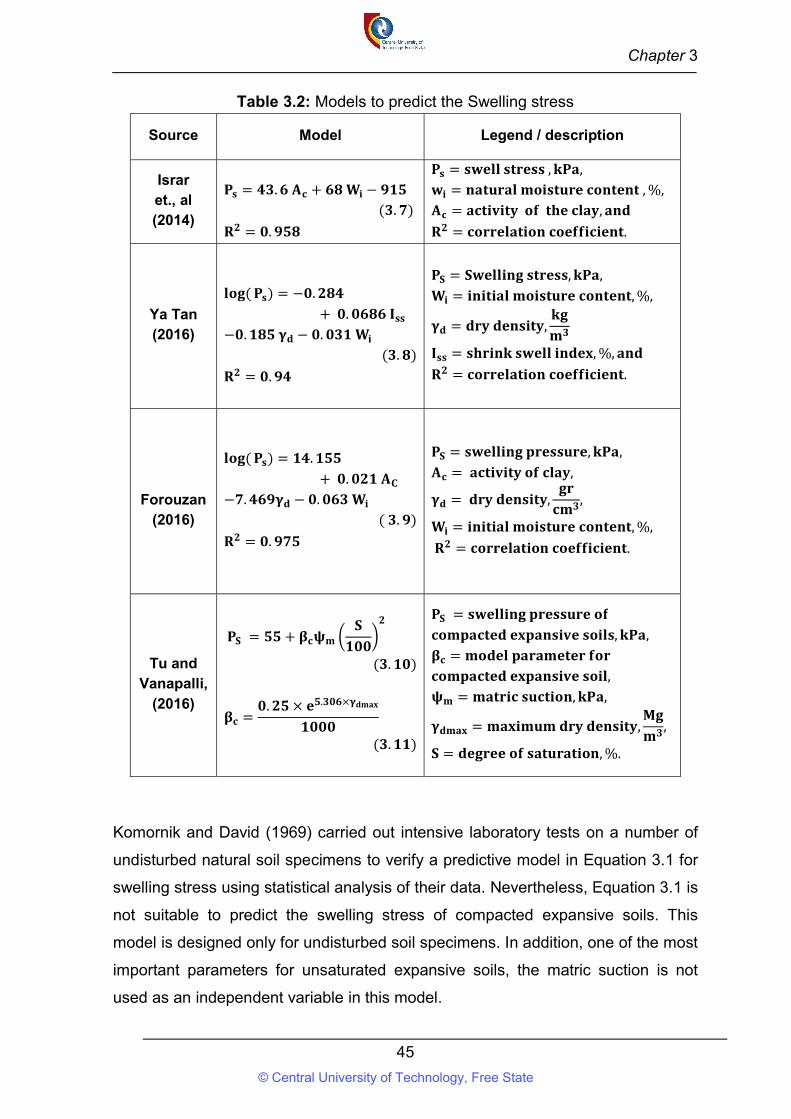
Chapter 3

45

Table 3.2: Models to predict the Swelling stress

Source Model Legend / description

Israr et., al (2014)

𝐏𝐬 = 𝟒𝟑. 𝟔 𝐀𝐜 + 𝟔𝟖 𝐖𝐢 − 𝟗𝟏𝟓 (𝟑. 𝟕)

𝐑𝟐 = 𝟎. 𝟗𝟓𝟖

𝐏𝐬 = 𝐬𝐰𝐞𝐥𝐥 𝐬𝐭𝐫𝐞𝐬𝐬 , 𝐤𝐏𝐚,

𝐰𝐢 = 𝐧𝐚𝐭𝐮𝐫𝐚𝐥 𝐦𝐨𝐢𝐬𝐭𝐮𝐫𝐞 𝐜𝐨𝐧𝐭𝐞𝐧𝐭 , %,

𝐀𝐜 = 𝐚𝐜𝐭𝐢𝐯𝐢𝐭𝐲 𝐨𝐟 𝐭𝐡𝐞 𝐜𝐥𝐚𝐲, 𝐚𝐧𝐝


Ya Tan (2016)

𝐥𝐨𝐠( 𝐏𝐬) = −𝟎. 𝟐𝟖𝟒

+ 𝟎. 𝟎𝟔𝟖𝟔 𝐈𝐬𝐬

−𝟎. 𝟏𝟖𝟓 𝛄𝐝 − 𝟎. 𝟎𝟑𝟏 𝐖𝐢

(𝟑. 𝟖)

𝐑𝟐 = 𝟎. 𝟗𝟒

𝐏𝐒 = 𝐒𝐰𝐞𝐥𝐥𝐢𝐧𝐠 𝐬𝐭𝐫𝐞𝐬𝐬, 𝐤𝐏𝐚,

𝐖𝐢 = 𝐢𝐧𝐢𝐭𝐢𝐚𝐥 𝐦𝐨𝐢𝐬𝐭𝐮𝐫𝐞 𝐜𝐨𝐧𝐭𝐞𝐧𝐭, %,

𝛄𝐝 = 𝐝𝐫𝐲 𝐝𝐞𝐧𝐬𝐢𝐭𝐲,𝐤𝐠

𝐦𝟑

𝐈𝐬𝐬 = 𝐬𝐡𝐫𝐢𝐧𝐤 𝐬𝐰𝐞𝐥𝐥 𝐢𝐧𝐝𝐞𝐱, %, 𝐚𝐧𝐝


Forouzan

(2016)

𝐥𝐨𝐠( 𝐏𝐬) = 𝟏𝟒. 𝟏𝟓𝟓

+ 𝟎. 𝟎𝟐𝟏 𝐀𝐂

−𝟕. 𝟒𝟔𝟗𝛄𝐝 − 𝟎. 𝟎𝟔𝟑 𝐖𝐢 ( 𝟑. 𝟗)

𝐑𝟐 = 𝟎. 𝟗𝟕𝟓

𝐏𝐒 = 𝐬𝐰𝐞𝐥𝐥𝐢𝐧𝐠 𝐩𝐫𝐞𝐬𝐬𝐮𝐫𝐞, 𝐤𝐏𝐚,

𝐀𝐜 = 𝐚𝐜𝐭𝐢𝐯𝐢𝐭𝐲 𝐨𝐟 𝐜𝐥𝐚𝐲,

𝛄𝐝 = 𝐝𝐫𝐲 𝐝𝐞𝐧𝐬𝐢𝐭𝐲,𝐠𝐫

𝐜𝐦𝟑,

𝐖𝐢 = 𝐢𝐧𝐢𝐭𝐢𝐚𝐥 𝐦𝐨𝐢𝐬𝐭𝐮𝐫𝐞 𝐜𝐨𝐧𝐭𝐞𝐧𝐭, %,


Tu and Vanapalli,

(2016)

𝐏𝐒 = 𝟓𝟓 + 𝛃𝐜𝛙𝐦

𝐒

𝟏𝟎𝟎

𝟐

(𝟑. 𝟏𝟎)

𝛃𝐜 =𝟎. 𝟐𝟓 × 𝐞𝟓.𝟑𝟎𝟔×𝛄𝐝𝐦𝐚𝐱

𝟏𝟎𝟎𝟎

(𝟑. 𝟏𝟏)

𝐏𝐒 = 𝐬𝐰𝐞𝐥𝐥𝐢𝐧𝐠 𝐩𝐫𝐞𝐬𝐬𝐮𝐫𝐞 𝐨𝐟

𝐜𝐨𝐦𝐩𝐚𝐜𝐭𝐞𝐝 𝐞𝐱𝐩𝐚𝐧𝐬𝐢𝐯𝐞 𝐬𝐨𝐢𝐥𝐬, 𝐤𝐏𝐚,

𝛃𝐜 = 𝐦𝐨𝐝𝐞𝐥 𝐩𝐚𝐫𝐚𝐦𝐞𝐭𝐞𝐫 𝐟𝐨𝐫

𝐜𝐨𝐦𝐩𝐚𝐜𝐭𝐞𝐝 𝐞𝐱𝐩𝐚𝐧𝐬𝐢𝐯𝐞 𝐬𝐨𝐢𝐥,

𝛙𝐦 = 𝐦𝐚𝐭𝐫𝐢𝐜 𝐬𝐮𝐜𝐭𝐢𝐨𝐧, 𝐤𝐏𝐚,

𝛄𝐝𝐦𝐚𝐱 = 𝐦𝐚𝐱𝐢𝐦𝐮𝐦 𝐝𝐫𝐲 𝐝𝐞𝐧𝐬𝐢𝐭𝐲,𝐌𝐠

𝐦𝟑,

𝐒 = 𝐝𝐞𝐠𝐫𝐞𝐞 𝐨𝐟 𝐬𝐚𝐭𝐮𝐫𝐚𝐭𝐢𝐨𝐧, %.

Komornik and David (1969) carried out intensive laboratory tests on a number of

undisturbed natural soil specimens to verify a predictive model in Equation 3.1 for

swelling stress using statistical analysis of their data. Nevertheless, Equation 3.1 is

not suitable to predict the swelling stress of compacted expansive soils. This

model is designed only for undisturbed soil specimens. In addition, one of the most

important parameters for unsaturated expansive soils, the matric suction is not

used as an independent variable in this model.


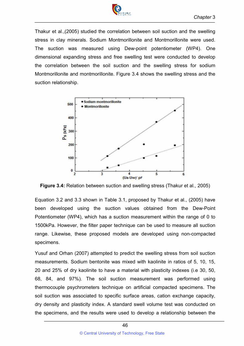
Chapter 3

46

Thakur et al.,(2005) studied the correlation between soil suction and the swelling

stress in clay minerals. Sodium Montmorillonite and Montmorillonite were used.

The suction was measured using Dew-point potentiometer (WP4). One

dimensional expanding stress and free swelling test were conducted to develop

the correlation between the soil suction and the swelling stress for sodium

Montmorillonite and montmorillonite. Figure 3.4 shows the swelling stress and the

suction relationship.

Figure 3.4: Relation between suction and swelling stress (Thakur et al., 2005)

Equation 3.2 and 3.3 shown in Table 3.1, proposed by Thakur et al., (2005) have

been developed using the suction values obtained from the Dew-Point

Potentiometer (WP4), which has a suction measurement within the range of 0 to

1500kPa. However, the filter paper technique can be used to measure all suction

range. Likewise, these proposed models are developed using non-compacted

specimens.

Yusuf and Orhan (2007) attempted to predict the swelling stress from soil suction

measurements. Sodium bentonite was mixed with kaolinite in ratios of 5, 10, 15,

20 and 25% of dry kaolinite to have a material with plasticity indexes (i.e 30, 50,

68, 84, and 97%). The soil suction measurement was performed using

thermocouple psychrometers technique on artificial compacted specimens. The

soil suction was associated to specific surface areas, cation exchange capacity,

dry density and plasticity index. A standard swell volume test was conducted on

the specimens, and the results were used to develop a relationship between the


Chapter 3

47

swelling stress and the logarithm of soil suction. The proposed equations 3.4 to 3.5

are shown in Table 3.1. The proposed models cannot predict a swelling stress

beyond 350 kPa. In addition, the models were design using artificial compacted

expansive soils made up by mixing sodium bentonite with Kaolinite. Hence, these

models are not suitable to predict precisely the swelling stress of field compacted

expansive soils.

Elisha (2012) performed one-dimensional swell tests on expansive clay mixed

with different percentages of kaolinite and bentonite to yield a wide range of

plasticity. Specimens were compacted at different initial water contents and dry

densities. Model Equation 3.6 shown in Table 3.1 use to predict the swelling stress

is based on three independent variables: plasticity index, water content and dry

density, and it is developed using multiple regression analysis. Soil suction is an

essential parameter for expansive soils. However, the model proposed by Elisha

(2012) is built up without the soil suction. The matric suction should have been

added as an independent variable in the model to enhance the prediction of the

swelling stress. Furthermore, the impact of the soil suction on the prediction of the

swelling stress was mentioned by Tu et al., (2016), they have developed a model

to predict the swelling stress of expansive soils using the soil suction values

obtained from the soil water characteristic curve (SWCC).

Israr et al., (2014) studied the correlations between the index properties and the

swelling stress of expansive soils, and the model Equation 3.7 in Table 3.2 was

developed to predict the swelling stress of expansive soils. The results given by

the proposed model were obtained with an accuracy of + 5% with respect to tests

values. The model proposed by Israr et al., (2014) is developed based on two

independent variables, the activity of clay, and initial water content. Even though

the predicted swelling stress was obtained with an accuracy of 5%, another

research work by Sridharan and Prakash (2000) concluded that the index

properties such as liquid limit, plasticity index, activity of the clay and related

parameters could not accurately predict the soil swelling behaviour of expansive

soils because they do not consider the effect of soil mineralogy. This model should

have been enhanced by adding the soil suction as an independent variable.


Chapter 3

48

Ya Tan (2016) conducted a series of oedometer test on expansive soils to

determine the swelling stress developed within the soil specimens upon initial

moisture content, dry density, and swell-shrink index. A multiple regression

analysis was performed to analyze the data obtained from the experiment and

develop model Equation 3.8 shown in Table 3.2 to predict the swelling stress. The

Plasticity Index and the soil suction are not used as an independent variable in

model Equation 3.8. Israr et al., (2014) pointed out that, the augmentation of the

plasticity index increases significantly the swelling stress of expansive soils.

Another research work conducted by Tu et al., (2016) revealed that the soil suction

is an important parameter in the prediction of the swelling stress. Because of the

variability of soil material, it would be beneficial to develop a model with many

relevant independent parameters for more accuracy. However, according to the

results of the study carried out by Sridharan and Prakash (1998) on expansive soil,

the swell/shrink index is a not good predictor of the swelling behaviour of fine-

grained soils because while the soil swelling stress is influenced by the presence

of the clay mineral, the soil shrinkage is a result of packing phenomenon and

controlled by the relative particle size distribution of fine-grained materials.

Forouzan (2016) developed mathematical model to predict the swelling stress of

expansive soils based on artificial soils made by mixing kaolinite and bentonite in

various proportions. Model Equation 3.9 is built with three independent variables:

the activity of clay, dry density, and initial water content. Other relevant parameters

to predict the swelling stress of expansive soil such as the soil suction had not

been used as independent variables in this model.

Tu et al., (2016) proposed a mathematical Equation 3.10 for the prediction of the

swelling stress of one - dimensional heave for expansive compacted soil with

respect to matric suction using the soil water characteristic curve (SWCC). The

matric suction can be used as a relevant independent variable to predict certain

behaviour of expansive soils like the swelling stress. The soil water characteristic

curve (SWCC) used to build up the model Equation 3.10 can be used to measure

soil suction, degree of saturation, water content (gravimetric or volumetric) but not

the maximum dry density as used in Equation 3.11 or other relevant soil

parameters that influence the swelling stress.


Chapter 3

49

Nevertheless, it is important to mention that the semi-empirical model proposed by

Tu et al., (2016) did not use only the matric suction as the independent variable.

The maximum dry density and the degree of saturation were used in Equation

3.10. Therefore, this model is not developed using only the matric suction, but by

using three independent variables. According to the precedent proposed models,

there are several other relevant soil parameters that influence significantly the

swelling stress. Therefore, it would be good to use a maximum of relevant

independent variables to develop an efficient predictive model.

3.5 Conclusion

Several models have been developed over the years to predict the swelling stress

of expansive soils, and the data used to develop the majority of these models were

collected from artificial specimen made up by a mixture of bentonite/kaolinite with

field soil. Soil compaction is widely used in construction to maximize the dry

density and achieve a desired strength. Nonetheless, few models to predict the

swelling stress were developed using field compacted expansive soils.

Furthermore, because of the variability of soil material, previous authors’ models

were developed for a specific type of soil material. Some models to predict the

swelling stress are summarized in Tables 3.1 and 3.2. These models were

developed using different types and different numbers of soil parameters as

independent variables, the number and the type of independent variables vary

from one model to another. These independent variables are as follows:

unsaturated soil characteristics (Matric suction, SWCC), geotechnical index

properties (initial dry density, Initial water content, plasticity index, liquid limit, and

activity of clay), expansive soil indexes (modified free swell index, swell/shrink

index). The majority of these models are developed with a minimum of two, and a

maximum of four independent variables. An increment of the number of

independent variables would improve the accuracy of the predictive models. To

enhance foundation design in expansive soils in Free State province, a correlation

between the swelling stress and other soils parameters must be investigated.

Furthermore, models used to predict the swelling stress of compacted expansive

soils have to be developed.


Chapter 4

50

CHAPTER 4: EXPERIMENTAL STUDY

4.1 Introduction

This research is based on experiments conducted in the geotechnical laboratory of

the department of the civil engineering at the Central University of Technology,

Free State. Additionally, X-ray diffraction tests were performed at the analytical

facility of the University of Johannesburg. In this chapter, the type test standard,

and the processes of experimental works are described.

The laboratory tests conducted to assess the physical and hydromechanical

properties of soils tested are as follows: Particle size distribution (sieve analysis,

hydrometer analysis), Atterberg limits, linear shrinkage, specific gravity, free swell

index, free swell ratio, X-ray diffraction, Proctor compaction test, swelling stress

test, soil suction estimation by filter paper technique, and the soil water

characteristic curve (SWCC).

The results obtained from laboratory tests are analyzed, discussed qualitatively

and quantitatively. The correlations between the swelling stress, the soil suction,

and other soil parameters are determined. Predictive models are developed by

multiple regression analysis using software NCSS11 to predict the swelling stress

of compacted expansive soils with respect to the soil suction, geotechnical index

properties, expansive soil indexes, and mineralogy characteristic. The validation of

the proposed models is achieved by comparing the predicted values to the values

obtained from experimental works, and by comparing the predicted values

obtained from the developed models to the values obtained from other existing

models.

4.2 Sample locations

Soil samples were collected from various locations across the province of Free

State (Petrusburg, Bloemfontein, Winburg, Welkom, and Bethlehem). The location

of sampling points are shown in Figure 4.1, and the samples collection from the

field is shown in Figure 4.2.


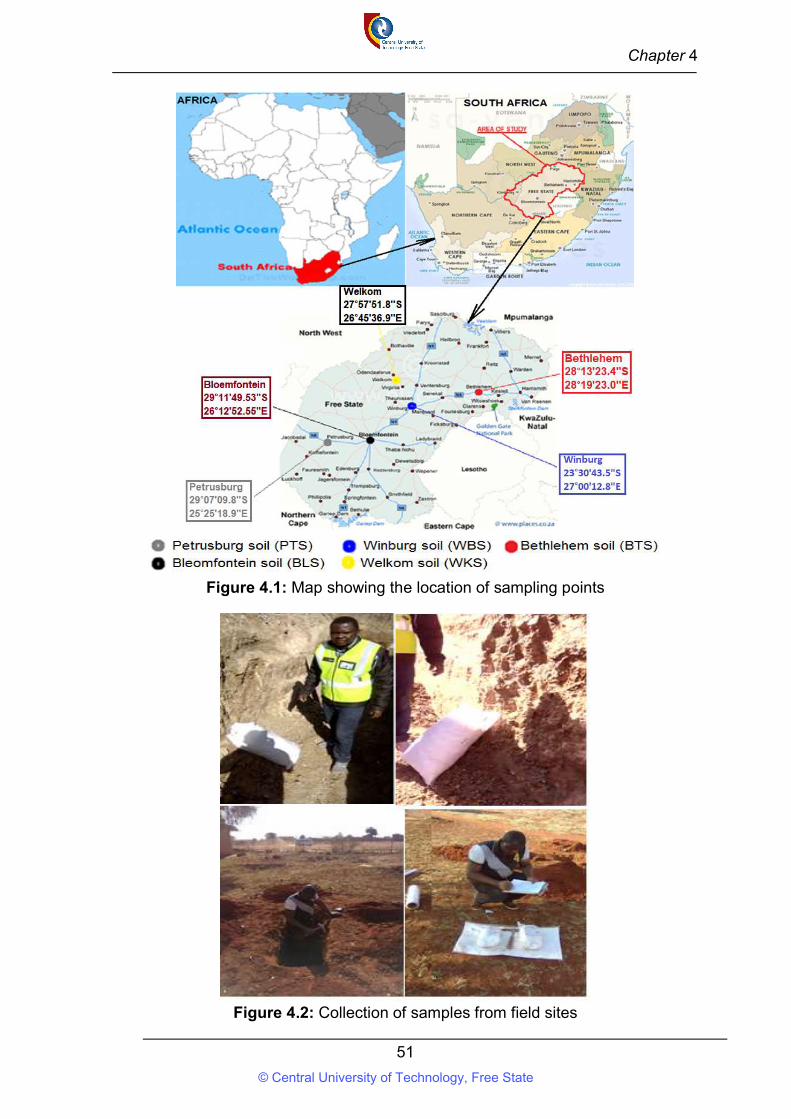
Chapter 4

51

Figure 4.1: Map showing the location of sampling points

Figure 4.2: Collection of samples from field sites


Chapter 4

52

4.3 Laboratory tests

The experimental standards used in this research work are summarized in

Table 4.1.

Table 4.1: Summary of test standards

No TEST REFERENCE

01 Particle size

distribution

Sieve analysis ATSM D6913

Hydrometer

analysis ATSM D7928

02 Atterberg

Limits

Liquid limit ASTM D4318

Plastic limit

03 Linear shrinkage Test TMH-1 Method A4

04 Free swell index of soil BIS, I. 1977

05 Identification of soil clay

mineralogy by free swell ratio

Sridharan & Prakash

( 2000)

06 X-Ray Diffraction (XRD) Brindley and Brown (1984)

07 Specific gravity test ASTM D854

08 Modified Proctor compaction TMH-1 Method A7

9 Swelling pressure test ASTM, D4546

10 Soil suction measurement ASTM D5298

11 Soil water characteristic curve

(SWCC)

Seki (2007)

Fredlund and Xing (1994)

Van Genuchten (1980)

4.3.1 Particle size distribution

Particle size distribution (PSD), known as soil gradation tests, were conducted on

particulate materials within the range of clay to boulders. This fundamental

experiment refers to discern the percentage of particles within a specified particle

size range across all the sizes represented for the soil samples. The distribution of

different grain sizes affects the engineering properties of soil, and it is required for

soil classification. The particle size distribution was conducted in accordance with

ASTM D6913 for sieve analysis, and ASTM D7928 for hydrometer analysis. The


Chapter 4

53

PSD was performed in two steps. In the first step, particle sizes greater than 75

μm (retained on the No. 200 sieve) were estimated by mechanical sieve analysis

Figure 5.3a. In the second step, the distribution of particle sizes smaller than 75

μm was estimated by sedimentation technique, using a hydrometer as shown in

Figure 5.3c.

4.3.2 Sieve Analysis

About 500g of oven dry soil sample was taken to perform sieve analysis. The

mass of each sieve as well as the bottom pan was recorded. Then, all the sieves

were cleaned and assembled in the ascending order of sieve number (# 4 sieve at

the top and #200 sieve at the bottom). The measured oven-dried sample was

poured into the top sieve, and covered with the lid. The sieve stack was placed on

the mechanical shaker and agitated for 10 minutes Figure 4.3a. After, the stack

was removed from the shaker, and carefully weighed to record the soil mass

retained in each sieve. The weight of the bottom pan with its retained fine soil was

measured. The soil mass retained on each sample was obtained by subtracting

the mass of the empty sieve from the mass of the sieve plus retained soil, and the

mass was recorded in a data sheet. The sum of the retained masses was

approximately the same as the initial mass for soils PTS, BLS, WBS, WKS, and

BTS used for the experiment. The percentage of the retained soil on each sieve

was obtained by dividing the retained mass on each sieve by the original mass.

The percentage of passing was obtained by starting with 100 percent and

subtracting the percent retained on each sieve in a cumulative process. After, a

semi-logarithmic graph of the grain size versus percent finer was plotted.

4.3.3 Hydrometer Analysis

Finer soil, silt and clay fraction (smaller than 75 μm) cannot be assessed by sieve

analysis. It is usually performed by sedimentation technique (hydrometer analysis).

The soil retained on the pan after sieve analysis was dried and about 100 g of soil

was taken for the hydrometer analysis. The specimen was mixed with 125 ml of

4% (NaPO3)6 (Sodium hexametaphosphate) solution in a small evaporating dish

and then, the dish was covered with a wet paper towel to reduce evaporation. The

mixture was kept for 16 hours to soak. After soaking, the mixture was transferred

to a dispersion cup, and water was added until the cup was around 2/3 full. After,


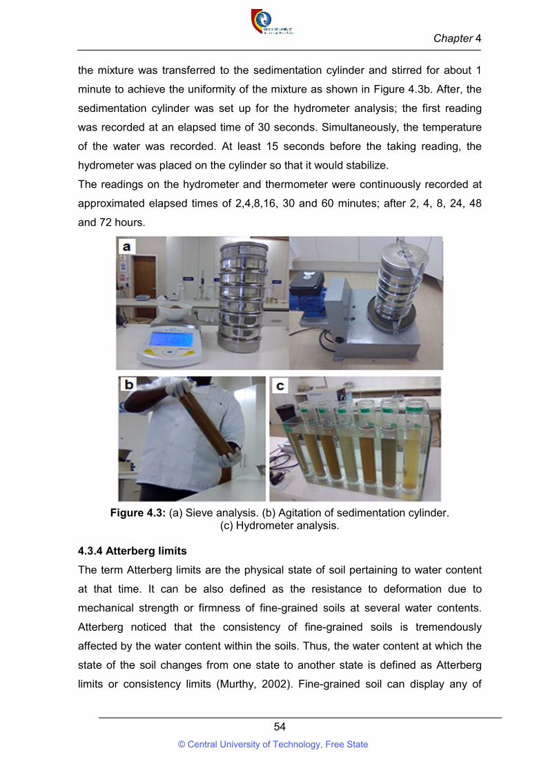
Chapter 4

54

the mixture was transferred to the sedimentation cylinder and stirred for about 1

minute to achieve the uniformity of the mixture as shown in Figure 4.3b. After, the

sedimentation cylinder was set up for the hydrometer analysis; the first reading

was recorded at an elapsed time of 30 seconds. Simultaneously, the temperature

of the water was recorded. At least 15 seconds before the taking reading, the

hydrometer was placed on the cylinder so that it would stabilize.

The readings on the hydrometer and thermometer were continuously recorded at

approximated elapsed times of 2,4,8,16, 30 and 60 minutes; after 2, 4, 8, 24, 48

and 72 hours.

Figure 4.3: (a) Sieve analysis. (b) Agitation of sedimentation cylinder.

(c) Hydrometer analysis.

4.3.4 Atterberg limits

The term Atterberg limits are the physical state of soil pertaining to water content

at that time. It can be also defined as the resistance to deformation due to

mechanical strength or firmness of fine-grained soils at several water contents.

Atterberg noticed that the consistency of fine-grained soils is tremendously

affected by the water content within the soils. Thus, the water content at which the

state of the soil changes from one state to another state is defined as Atterberg

limits or consistency limits (Murthy, 2002). Fine-grained soil can display any of


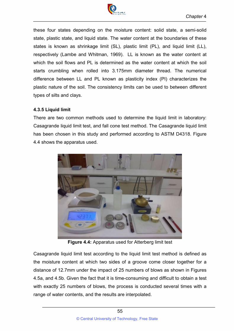
Chapter 4

55

these four states depending on the moisture content: solid state, a semi-solid

state, plastic state, and liquid state. The water content at the boundaries of these

states is known as shrinkage limit (SL), plastic limit (PL), and liquid limit (LL),

respectively (Lambe and Whitman, 1969). LL is known as the water content at

which the soil flows and PL is determined as the water content at which the soil

starts crumbling when rolled into 3.175mm diameter thread. The numerical

difference between LL and PL known as plasticity index (PI) characterizes the

plastic nature of the soil. The consistency limits can be used to between different

types of silts and clays.

4.3.5 Liquid limit

There are two common methods used to determine the liquid limit in laboratory:

Casagrande liquid limit test, and fall cone test method. The Casagrande liquid limit

has been chosen in this study and performed according to ASTM D4318. Figure

4.4 shows the apparatus used.

Figure 4.4: Apparatus used for Atterberg limit test

Casagrande liquid limit test according to the liquid limit test method is defined as

the moisture content at which two sides of a groove come closer together for a

distance of 12.7mm under the impact of 25 numbers of blows as shown in Figures

4.5a, and 4.5b. Given the fact that it is time-consuming and difficult to obtain a test

with exactly 25 numbers of blows, the process is conducted several times with a

range of water contents, and the results are interpolated.


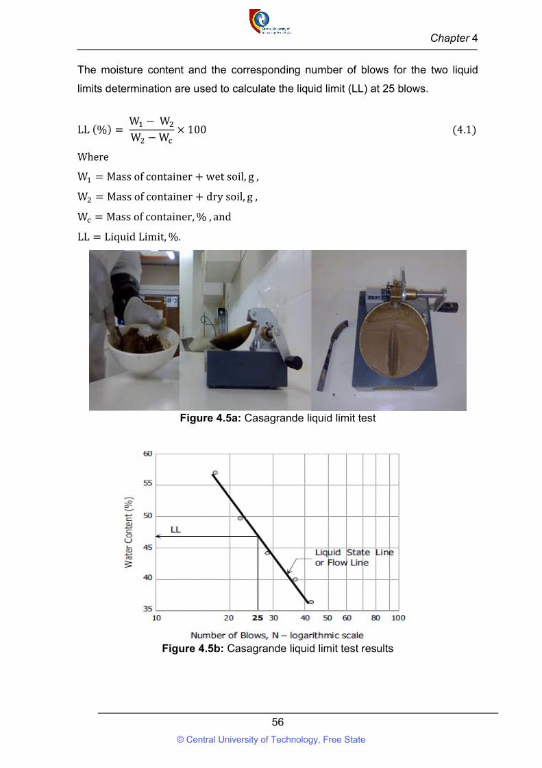
Chapter 4

56

The moisture content and the corresponding number of blows for the two liquid

limits determination are used to calculate the liquid limit (LL) at 25 blows.

LL (%) = W − W

W − W× 100 (4.1)

Where

W = Mass of container + wet soil, g ,

W = Mass of container + dry soil, g ,

W = Mass of container, % , and

LL = Liquid Limit, %.

Figure 4.5a: Casagrande liquid limit test

Figure 4.5b: Casagrande liquid limit test results


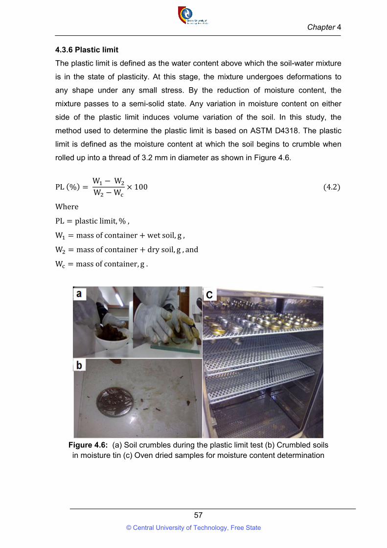
Chapter 4

57

4.3.6 Plastic limit

The plastic limit is defined as the water content above which the soil-water mixture

is in the state of plasticity. At this stage, the mixture undergoes deformations to

any shape under any small stress. By the reduction of moisture content, the

mixture passes to a semi-solid state. Any variation in moisture content on either

side of the plastic limit induces volume variation of the soil. In this study, the

method used to determine the plastic limit is based on ASTM D4318. The plastic

limit is defined as the moisture content at which the soil begins to crumble when

rolled up into a thread of 3.2 mm in diameter as shown in Figure 4.6.

PL (%) = W − W

W − W× 100 (4.2)

Where

PL = plastic limit, % ,

W = mass of container + wet soil, g ,

W = mass of container + dry soil, g , and

W = mass of container, g .

Figure 4.6: (a) Soil crumbles during the plastic limit test (b) Crumbled soils in moisture tin (c) Oven dried samples for moisture content determination


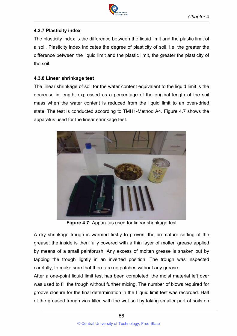
Chapter 4

58

4.3.7 Plasticity index

The plasticity index is the difference between the liquid limit and the plastic limit of

a soil. Plasticity index indicates the degree of plasticity of soil, i.e. the greater the

difference between the liquid limit and the plastic limit, the greater the plasticity of

the soil.

4.3.8 Linear shrinkage test

The linear shrinkage of soil for the water content equivalent to the liquid limit is the

decrease in length, expressed as a percentage of the original length of the soil

mass when the water content is reduced from the liquid limit to an oven-dried

state. The test is conducted according to TMH1-Method A4. Figure 4.7 shows the

apparatus used for the linear shrinkage test.

Figure 4.7: Apparatus used for linear shrinkage test

A dry shrinkage trough is warmed firstly to prevent the premature setting of the

grease; the inside is then fully covered with a thin layer of molten grease applied

by means of a small paintbrush. Any excess of molten grease is shaken out by

tapping the trough lightly in an inverted position. The trough was inspected

carefully, to make sure that there are no patches without any grease.

After a one-point liquid limit test has been completed, the moist material left over

was used to fill the trough without further mixing. The number of blows required for

groove closure for the final determination in the Liquid limit test was recorded. Half

of the greased trough was filled with the wet soil by taking smaller part of soils on


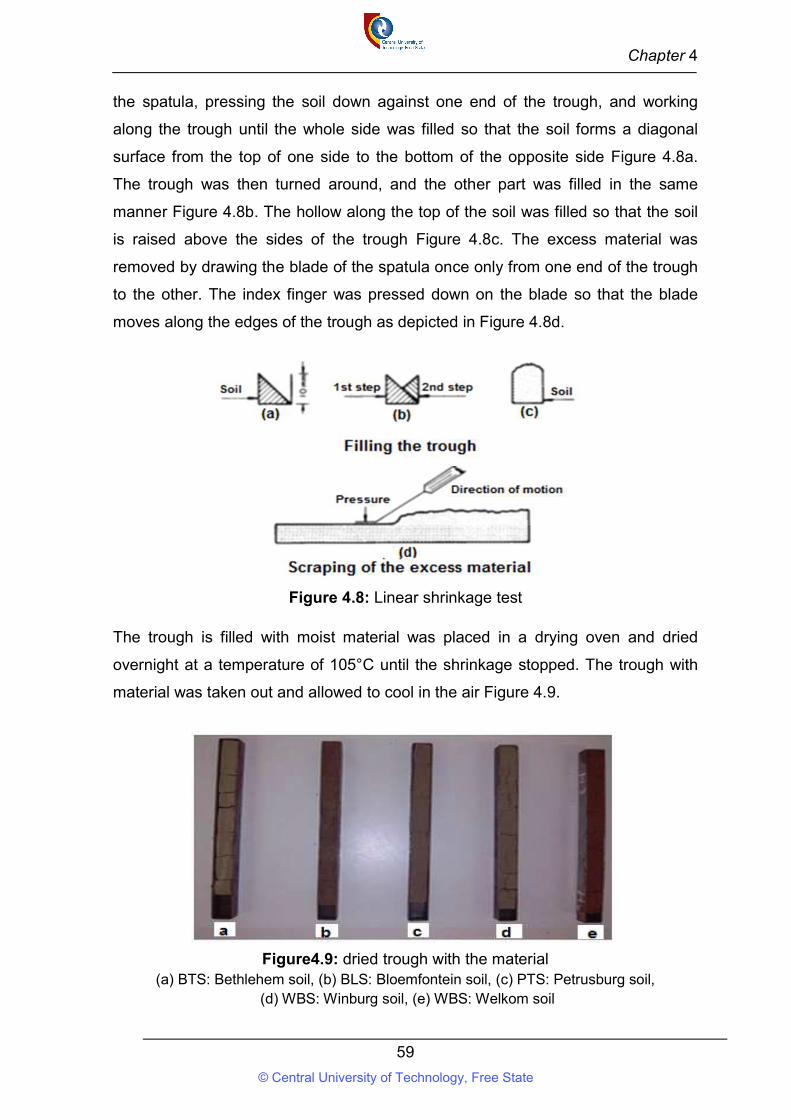
Chapter 4

59

the spatula, pressing the soil down against one end of the trough, and working

along the trough until the whole side was filled so that the soil forms a diagonal

surface from the top of one side to the bottom of the opposite side Figure 4.8a.

The trough was then turned around, and the other part was filled in the same

manner Figure 4.8b. The hollow along the top of the soil was filled so that the soil

is raised above the sides of the trough Figure 4.8c. The excess material was

removed by drawing the blade of the spatula once only from one end of the trough

to the other. The index finger was pressed down on the blade so that the blade

moves along the edges of the trough as depicted in Figure 4.8d.

Figure 4.8: Linear shrinkage test

The trough is filled with moist material was placed in a drying oven and dried

overnight at a temperature of 105°C until the shrinkage stopped. The trough with

material was taken out and allowed to cool in the air Figure 4.9.

Figure4.9: dried trough with the material

(a) BTS: Bethlehem soil, (b) BLS: Bloemfontein soil, (c) PTS: Petrusburg soil, (d) WBS: Winburg soil, (e) WBS: Welkom soil


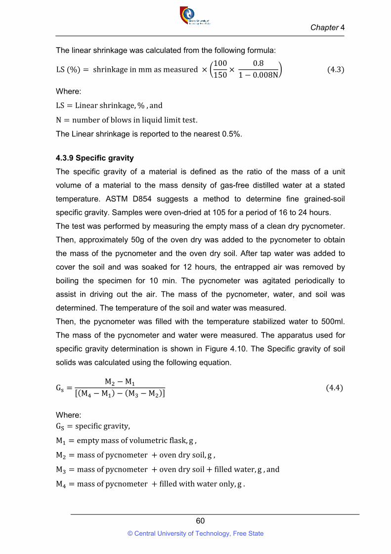
Chapter 4

60

The linear shrinkage was calculated from the following formula:

LS (%) = shrinkage in mm as measured ×100

150×

0.8

1 − 0.008N (4.3)

Where:

LS = Linear shrinkage, % , and

N = number of blows in liquid limit test.

The Linear shrinkage is reported to the nearest 0.5%.

4.3.9 Specific gravity

The specific gravity of a material is defined as the ratio of the mass of a unit

volume of a material to the mass density of gas-free distilled water at a stated

temperature. ASTM D854 suggests a method to determine fine grained-soil

specific gravity. Samples were oven-dried at 105 for a period of 16 to 24 hours.

The test was performed by measuring the empty mass of a clean dry pycnometer.

Then, approximately 50g of the oven dry was added to the pycnometer to obtain

the mass of the pycnometer and the oven dry soil. After tap water was added to

cover the soil and was soaked for 12 hours, the entrapped air was removed by

boiling the specimen for 10 min. The pycnometer was agitated periodically to

assist in driving out the air. The mass of the pycnometer, water, and soil was

determined. The temperature of the soil and water was measured.

Then, the pycnometer was filled with the temperature stabilized water to 500ml.

The mass of the pycnometer and water were measured. The apparatus used for

specific gravity determination is shown in Figure 4.10. The Specific gravity of soil

solids was calculated using the following equation.

G =M − M

[(M − M ) − (M − M )] (4.4)

Where: G = specific gravity,

M = empty mass of volumetric flask, g ,

M = mass of pycnometer + oven dry soil, g ,

M = mass of pycnometer + oven dry soil + filled water, g , and

M = mass of pycnometer + filled with water only, g .


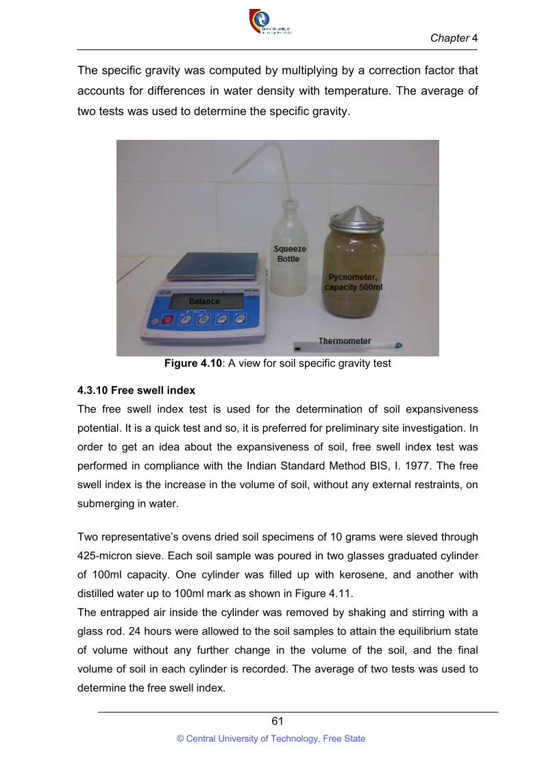
Chapter 4

61

The specific gravity was computed by multiplying by a correction factor that

accounts for differences in water density with temperature. The average of

two tests was used to determine the specific gravity.

Figure 4.10: A view for soil specific gravity test

4.3.10 Free swell index

The free swell index test is used for the determination of soil expansiveness

potential. It is a quick test and so, it is preferred for preliminary site investigation. In

order to get an idea about the expansiveness of soil, free swell index test was

performed in compliance with the Indian Standard Method BIS, I. 1977. The free

swell index is the increase in the volume of soil, without any external restraints, on

submerging in water.

Two representative’s ovens dried soil specimens of 10 grams were sieved through

425-micron sieve. Each soil sample was poured in two glasses graduated cylinder

of 100ml capacity. One cylinder was filled up with kerosene, and another with

distilled water up to 100ml mark as shown in Figure 4.11.

The entrapped air inside the cylinder was removed by shaking and stirring with a

glass rod. 24 hours were allowed to the soil samples to attain the equilibrium state

of volume without any further change in the volume of the soil, and the final

volume of soil in each cylinder is recorded. The average of two tests was used to

determine the free swell index.


Chapter 4

62

Figure 4.11: Free swelling test: (a) BTS: Bethlehem soil, (b) WKS: Welkom soil, (c) PTS: Petrusburg soil, (d) BLS: Bloemfontein soil; (e) WBS: Winburg soil

The free swell Index was calculated from the following equation.

FSI (%) =V − V

V× 100 (4.5)

Where:

FSI = free swell index, % ,

V = volume of the soil specimen read from the graduated cylinder

containing distilled water, ml, and

V = volume of the soil specimen read from the graduated cylinder

containing kerosene, ml.


Chapter 4

63

4.3.11 Free swell ratio and clay mineralogy

This test is used to assess the soil expansivity, and the type of dominant clay

mineral. According to the study conducted by Sridharan and Prakash (2000), free

swell ratio (FSR) method is a very competitive method that required a simple

procedure to assess the swell potential of expansive soil and the clay mineralogy.

The procedure is the same as the Free swell index test. The Free swell ratio was

determined using the following equation.

FSR =V

V (4.6)

Where:

FSR = free swell ratio,

V = volume of soil specimen read from graduated cylinder

containing distilled water, ml, and

V = volume of soil specimen read from graduated cylinder

containing kerosene, ml .

Table 4.2 was used to classify the degree of expansivity of the soil based on their

FSR. On the other hand, Table 4.2 was also used to identify the dominant clay

mineral.

Table 4.2: Classification of soil based on FSR (Sridharan & Prakash, 2000)

Free Swell Ratio

Clay Type Soil

Expansivity Dominant clay Mineral

Type

=1 Non - swelling Negligible Kaolinite

1.0 - 1.5 Mixture of swelling and non - swelling

Low Mixture of Kaolinitic and Montmorillonitic

1.5 - 2.0 Swelling Moderate Montmorillonitic 2.0 - 4.0 Swelling High Montmorillonitic

> 4.0 Swelling Very High Montmorillonitic

The free swell ratio method has been shown to be a simple and user-friendly

method that can be adopted in the field for characterizing the expansive soil, and

for the identification of their mineralogical composition.


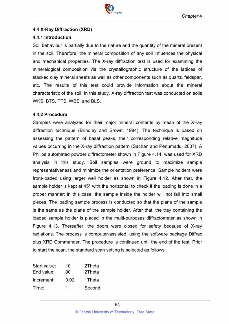
Chapter 4

64

4.4 X-Ray Diffraction (XRD)

4.4.1 Introduction

Soil behaviour is partially due to the nature and the quantity of the mineral present

in the soil. Therefore, the mineral composition of any soil influences the physical

and mechanical properties. The X-ray diffraction test is used for examining the

mineralogical composition via the crystallographic structure of the lattices of

stacked clay mineral sheets as well as other components such as quartz, feldspar,

etc. The results of this test could provide information about the mineral

characteristic of the soil. In this study, X-ray diffraction test was conducted on soils

WKS, BTS, PTS, WBS, and BLS.

4.4.2 Procedure

Samples were analyzed for their major mineral contents by mean of the X-ray

diffraction technique (Brindley and Brown, 1984). The technique is based on

assessing the pattern of basal peaks, their corresponding relative magnitude

values occurring in the X-ray diffraction pattern (Sachan and Penumadu, 2007). A

Philips automated powder diffractometer shown in Figure 4.14, was used for XRD

analysis in this study. Soil samples were ground to maximize sample

representativeness and minimize the orientation preference. Sample holders were

front-loaded using larger well holder as shown in Figure 4.12. After that, the

sample holder is kept at 45° with the horizontal to check if the loading is done in a

proper manner; in this case, the sample inside the holder will not fall into small

pieces. The loading sample process is conducted so that the plane of the sample

is the same as the plane of the sample holder. After that, the tray containing the

loaded sample holder is placed in the multi-purposes diffractometer as shown in

Figure 4.13. Thereafter, the doors were closed for safety because of X-ray

radiations. The process is computer-assisted, using the software package Diffrac

plus XRD Commander. The procedure is continued until the end of the test. Prior

to start the scan, the standard scan setting is selected as follows:

Start value: 10 2Theta End value: 90 2Theta

Increment: 0.02 1Theta

Time: 1 Second.


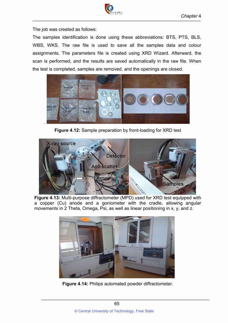
Chapter 4

65

The job was created as follows:

The samples identification is done using these abbreviations: BTS, PTS, BLS,

WBS, WKS. The raw file is used to save all the samples data and colour

assignments. The parameters file is created using XRD Wizard. Afterward, the

scan is performed, and the results are saved automatically in the raw file. When

the test is completed, samples are removed, and the openings are closed.

.

Figure 4.12: Sample preparation by front-loading for XRD test

Figure 4.13: Multi-purpose diffractometer (MPD) used for XRD test equipped with a copper (Cu) anode and a goniometer with the cradle, allowing angular movements in 2 Theta, Omega, Psi, as well as linear positioning in x, y, and z.

Figure 4.14: Philips automated powder diffractometer.


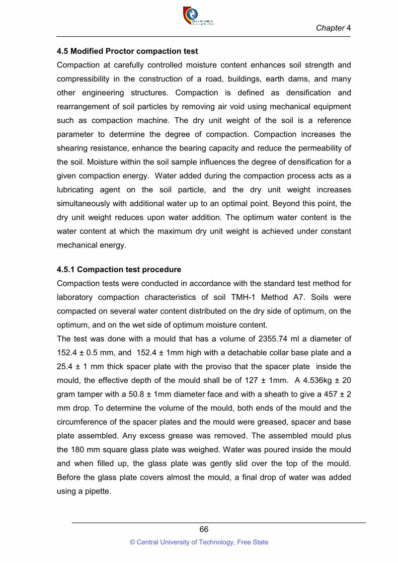
Chapter 4

66

4.5 Modified Proctor compaction test

Compaction at carefully controlled moisture content enhances soil strength and

compressibility in the construction of a road, buildings, earth dams, and many

other engineering structures. Compaction is defined as densification and

rearrangement of soil particles by removing air void using mechanical equipment

such as compaction machine. The dry unit weight of the soil is a reference

parameter to determine the degree of compaction. Compaction increases the

shearing resistance, enhance the bearing capacity and reduce the permeability of

the soil. Moisture within the soil sample influences the degree of densification for a

given compaction energy. Water added during the compaction process acts as a

lubricating agent on the soil particle, and the dry unit weight increases

simultaneously with additional water up to an optimal point. Beyond this point, the

dry unit weight reduces upon water addition. The optimum water content is the

water content at which the maximum dry unit weight is achieved under constant

mechanical energy.

4.5.1 Compaction test procedure

Compaction tests were conducted in accordance with the standard test method for

laboratory compaction characteristics of soil TMH-1 Method A7. Soils were

compacted on several water content distributed on the dry side of optimum, on the

optimum, and on the wet side of optimum moisture content.

The test was done with a mould that has a volume of 2355.74 ml a diameter of

152.4 ± 0.5 mm, and 152.4 ± 1mm high with a detachable collar base plate and a

25.4 ± 1 mm thick spacer plate with the proviso that the spacer plate inside the

mould, the effective depth of the mould shall be of 127 ± 1mm. A 4.536kg ± 20

gram tamper with a 50.8 ± 1mm diameter face and with a sheath to give a 457 ± 2

mm drop. To determine the volume of the mould, both ends of the mould and the

circumference of the spacer plates and the mould were greased, spacer and base

plate assembled. Any excess grease was removed. The assembled mould plus

the 180 mm square glass plate was weighed. Water was poured inside the mould

and when filled up, the glass plate was gently slid over the top of the mould.

Before the glass plate covers almost the mould, a final drop of water was added

using a pipette.


Chapter 4

67

The mould with water and glass plate were weighed, and the mass of water in the

mould computed. The temperature of the water was measured, and the volume of

the mould was computed as follows:

V =Mass of water in gram

RD of water at test temperature (4.7)

Where:

V = volume of the mould, ml, and

RD = relative density of water according to temperature.

Table 4.3: Relative density of water according to temperature

Temp.oC RD of water Temp.oC RD of water

15 0.99913 23 0.99756 16 0.99897 24 0.99732 17 0.99880 25 0.99707 18 0.99862 26 0.99681 19 0.99843 27 0.99654 20 0.99823 28 0.99626 21 0.99802 29 0.99597 22 0.99780 30 0.99567

Samples were sieved through 425-micron sieve; approximately 35 kg of the

sample was oven-dried at 105°C for a period of 16 to 24 hours and divided to

obtain five basins of exactly similar material.

The specific mass of water to be added to the material in the basin was calculated

using Equation 4.8. While adding water, the material was mixed continuously with

a trowel.

M =M (W − W )

100 (4.8)

Where

M = mass of water to be added , g ,

M = mass of the dry soil , g ,

W = targeted moisture content , % , and

W = initial moisture content, % .


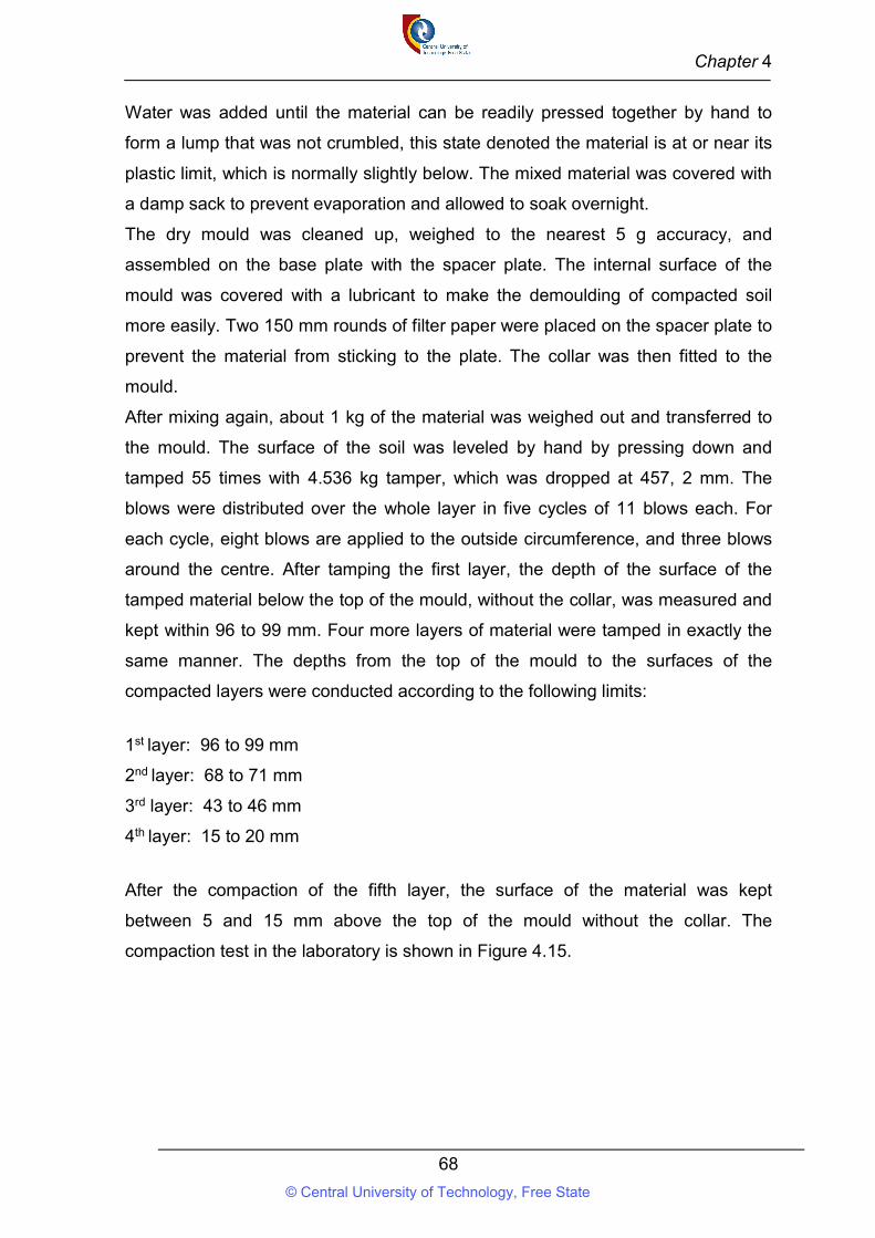
Chapter 4

68

Water was added until the material can be readily pressed together by hand to

form a lump that was not crumbled, this state denoted the material is at or near its

plastic limit, which is normally slightly below. The mixed material was covered with

a damp sack to prevent evaporation and allowed to soak overnight.

The dry mould was cleaned up, weighed to the nearest 5 g accuracy, and

assembled on the base plate with the spacer plate. The internal surface of the

mould was covered with a lubricant to make the demoulding of compacted soil

more easily. Two 150 mm rounds of filter paper were placed on the spacer plate to

prevent the material from sticking to the plate. The collar was then fitted to the

mould.

After mixing again, about 1 kg of the material was weighed out and transferred to

the mould. The surface of the soil was leveled by hand by pressing down and

tamped 55 times with 4.536 kg tamper, which was dropped at 457, 2 mm. The

blows were distributed over the whole layer in five cycles of 11 blows each. For

each cycle, eight blows are applied to the outside circumference, and three blows

around the centre. After tamping the first layer, the depth of the surface of the

tamped material below the top of the mould, without the collar, was measured and

kept within 96 to 99 mm. Four more layers of material were tamped in exactly the

same manner. The depths from the top of the mould to the surfaces of the

compacted layers were conducted according to the following limits:

1st layer: 96 to 99 mm

2nd layer: 68 to 71 mm

3rd layer: 43 to 46 mm

4th layer: 15 to 20 mm

After the compaction of the fifth layer, the surface of the material was kept

between 5 and 15 mm above the top of the mould without the collar. The

compaction test in the laboratory is shown in Figure 4.15.


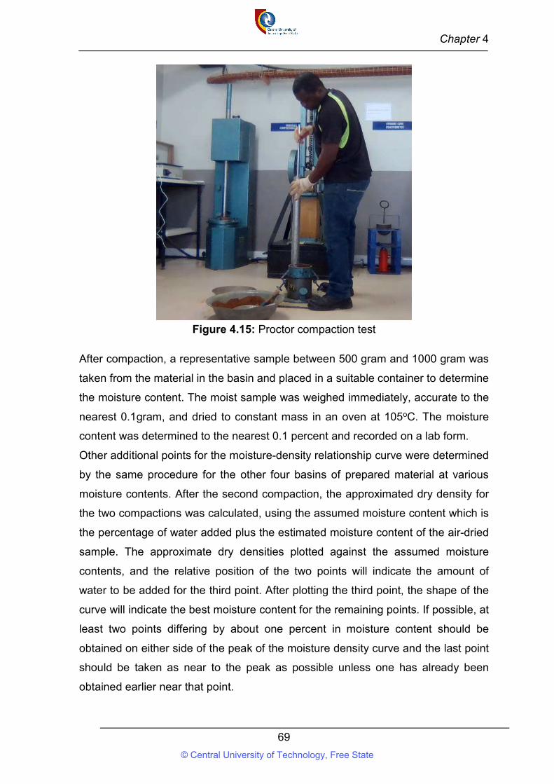
Chapter 4

69

Figure 4.15: Proctor compaction test

After compaction, a representative sample between 500 gram and 1000 gram was

taken from the material in the basin and placed in a suitable container to determine

the moisture content. The moist sample was weighed immediately, accurate to the

nearest 0.1gram, and dried to constant mass in an oven at 105oC. The moisture

content was determined to the nearest 0.1 percent and recorded on a lab form.

Other additional points for the moisture-density relationship curve were determined

by the same procedure for the other four basins of prepared material at various

moisture contents. After the second compaction, the approximated dry density for

the two compactions was calculated, using the assumed moisture content which is

the percentage of water added plus the estimated moisture content of the air-dried

sample. The approximate dry densities plotted against the assumed moisture

contents, and the relative position of the two points will indicate the amount of

water to be added for the third point. After plotting the third point, the shape of the

curve will indicate the best moisture content for the remaining points. If possible, at

least two points differing by about one percent in moisture content should be

obtained on either side of the peak of the moisture density curve and the last point

should be taken as near to the peak as possible unless one has already been

obtained earlier near that point.


Chapter 4

70

4.5.2 Calculation of compaction test parameters

The moisture content of the material was calculated using the average of the water

contents for each point to the nearest 0.1 % according to Equation 4.9

W(%) =(W − W )

(W − W ) × 100 (4.9)

Where:

W = mass of container + wet soil , g ,

W = mass of container + dry soil , g ,

W − W = mass of water , g ,

W − W = mass of the oven dry soil , g, and

W = moisture content, %.

The total density in kg/m3 of the compacted soil sample were determined by

dividing the wet mass by the volume of the mould used for each point

corresponding to a specific moisture content using Equation 4.10.

γ = (M − M )

V (4.10)

Where:

M = mass of mold, base plate, and wet soil , (kg),

M = mass of mold and base plate , (kg),

V = volume of the mould , (m ), and

γ = total density , (kg. m ).

The dry density of the material was determined for each point corresponding to a

specific moisture content using Equation 4.11.

γ =γ

1 + W

100

(4.11)

Where:

γ = total density, (kg. m ),

γ = dry density , (kg. m ), and

W = moisture content in , (%).


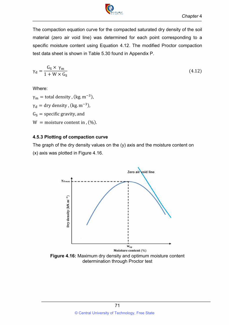
Chapter 4

71

The compaction equation curve for the compacted saturated dry density of the soil

material (zero air void line) was determined for each point corresponding to a

specific moisture content using Equation 4.12. The modified Proctor compaction

test data sheet is shown in Table 5.30 found in Appendix P.

γ =G × γ

1 + W × G (4.12)

Where:

γ = total density , (kg. m ),

γ = dry density , (kg. m ),

G = specific gravity, and

W = moisture content in , (%).

4.5.3 Plotting of compaction curve

The graph of the dry density values on the (y) axis and the moisture content on

(x) axis was plotted in Figure 4.16.

Figure 4.16: Maximum dry density and optimum moisture content

determination through Proctor test


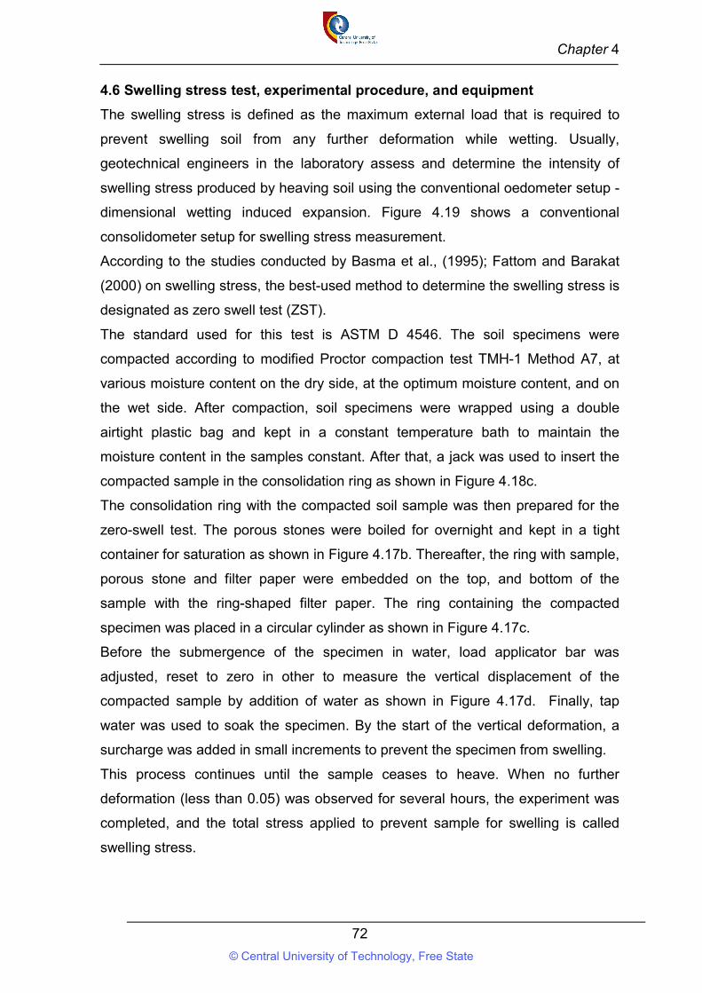
Chapter 4

72

4.6 Swelling stress test, experimental procedure, and equipment

The swelling stress is defined as the maximum external load that is required to

prevent swelling soil from any further deformation while wetting. Usually,

geotechnical engineers in the laboratory assess and determine the intensity of

swelling stress produced by heaving soil using the conventional oedometer setup -

dimensional wetting induced expansion. Figure 4.19 shows a conventional

consolidometer setup for swelling stress measurement.

According to the studies conducted by Basma et al., (1995); Fattom and Barakat

(2000) on swelling stress, the best-used method to determine the swelling stress is

designated as zero swell test (ZST).

The standard used for this test is ASTM D 4546. The soil specimens were

compacted according to modified Proctor compaction test TMH-1 Method A7, at

various moisture content on the dry side, at the optimum moisture content, and on

the wet side. After compaction, soil specimens were wrapped using a double

airtight plastic bag and kept in a constant temperature bath to maintain the

moisture content in the samples constant. After that, a jack was used to insert the

compacted sample in the consolidation ring as shown in Figure 4.18c.

The consolidation ring with the compacted soil sample was then prepared for the

zero-swell test. The porous stones were boiled for overnight and kept in a tight

container for saturation as shown in Figure 4.17b. Thereafter, the ring with sample,

porous stone and filter paper were embedded on the top, and bottom of the

sample with the ring-shaped filter paper. The ring containing the compacted

specimen was placed in a circular cylinder as shown in Figure 4.17c.

Before the submergence of the specimen in water, load applicator bar was

adjusted, reset to zero in other to measure the vertical displacement of the

compacted sample by addition of water as shown in Figure 4.17d. Finally, tap

water was used to soak the specimen. By the start of the vertical deformation, a

surcharge was added in small increments to prevent the specimen from swelling.

This process continues until the sample ceases to heave. When no further

deformation (less than 0.05) was observed for several hours, the experiment was

completed, and the total stress applied to prevent sample for swelling is called

swelling stress.


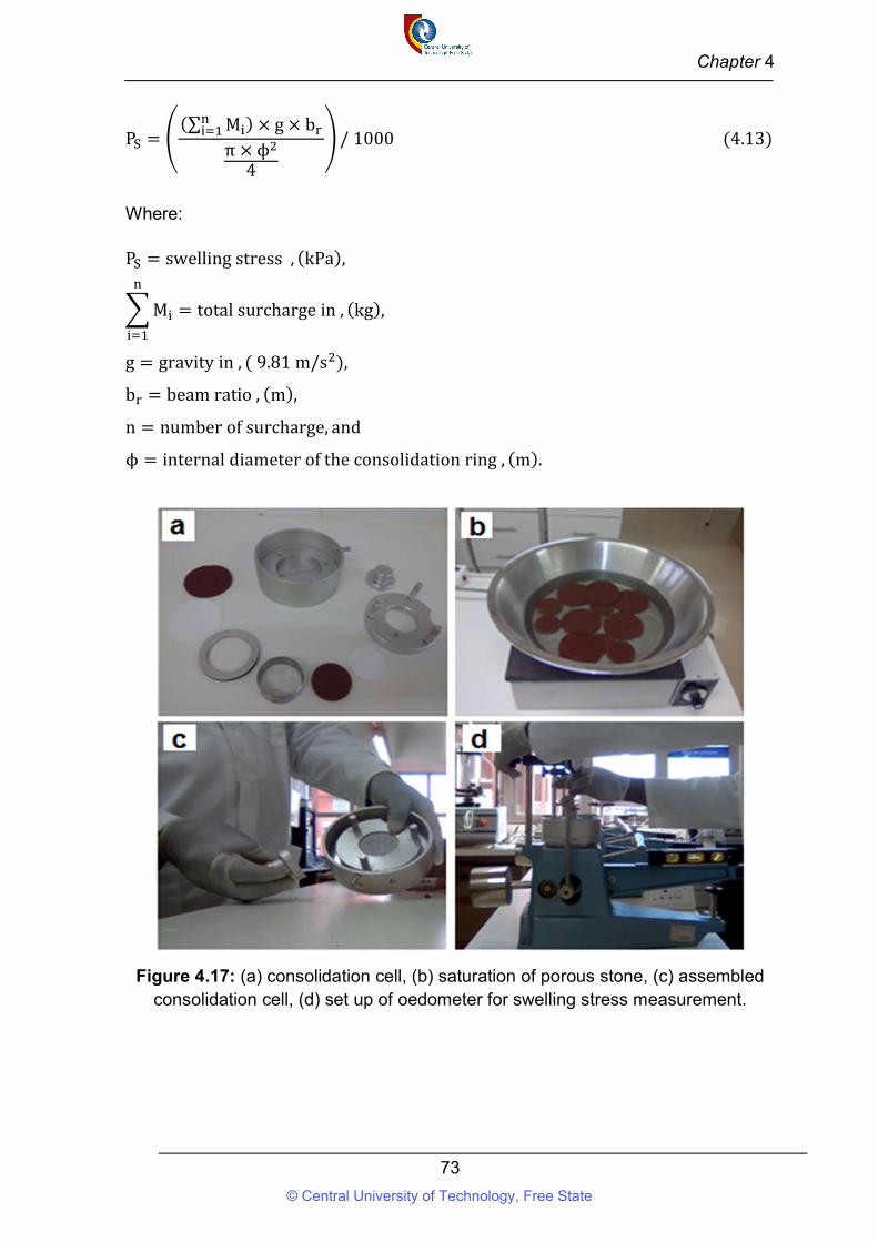
Chapter 4

73

P =(∑ M ) × g × b

π × ϕ4

/ 1000 (4.13)

Where: P = swelling stress , (kPa),

M = total surcharge in , (kg),

g = gravity in , ( 9.81 m/s ),

b = beam ratio , (m),

n = number of surcharge, and

ϕ = internal diameter of the consolidation ring , (m).

Figure 4.17: (a) consolidation cell, (b) saturation of porous stone, (c) assembled consolidation cell, (d) set up of oedometer for swelling stress measurement.


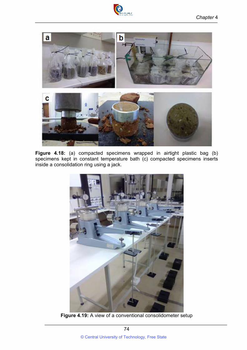
Chapter 4

74

Figure 4.18: (a) compacted specimens wrapped in airtight plastic bag (b) specimens kept in constant temperature bath (c) compacted specimens inserts inside a consolidation ring using a jack.

Figure 4.19: A view of a conventional consolidometer setup


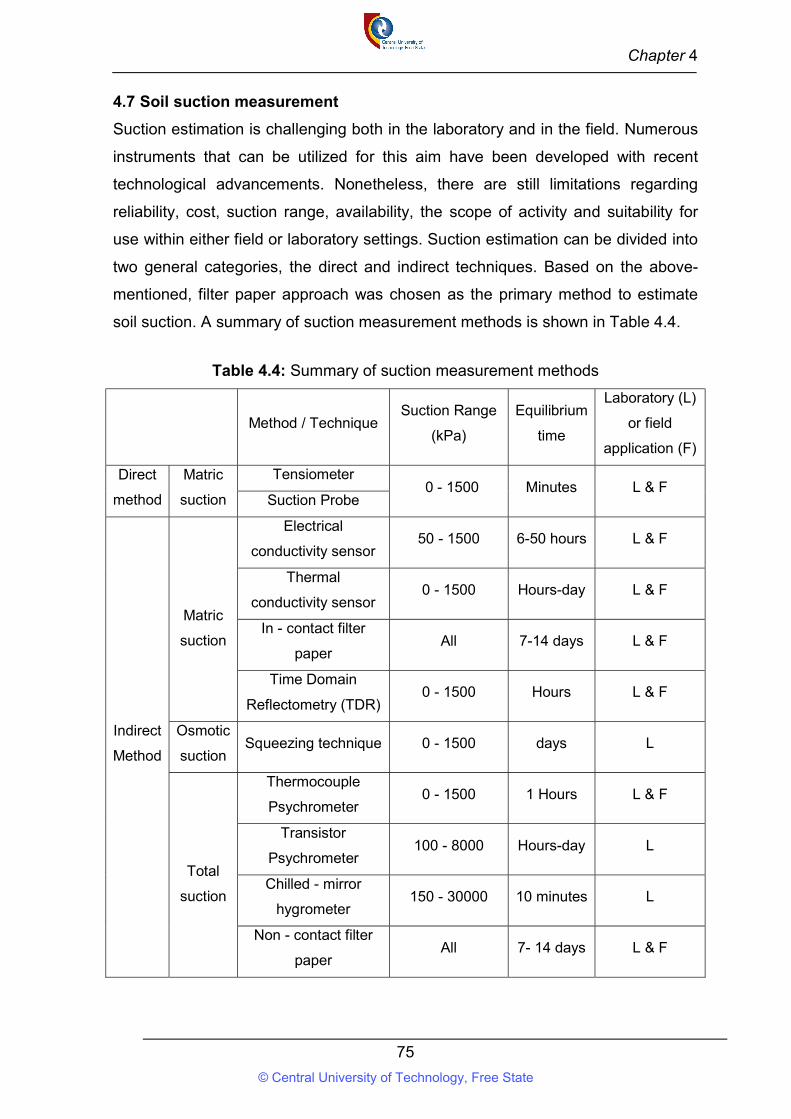
Chapter 4

75

4.7 Soil suction measurement

Suction estimation is challenging both in the laboratory and in the field. Numerous

instruments that can be utilized for this aim have been developed with recent

technological advancements. Nonetheless, there are still limitations regarding

reliability, cost, suction range, availability, the scope of activity and suitability for

use within either field or laboratory settings. Suction estimation can be divided into

two general categories, the direct and indirect techniques. Based on the above-

mentioned, filter paper approach was chosen as the primary method to estimate

soil suction. A summary of suction measurement methods is shown in Table 4.4.

Table 4.4: Summary of suction measurement methods

Method / Technique Suction Range

(kPa)

Equilibrium

time

Laboratory (L)

or field

application (F)

Direct

method

Matric

suction

Tensiometer 0 - 1500 Minutes L & F

Suction Probe

Indirect

Method

Matric

suction

Electrical

conductivity sensor 50 - 1500 6-50 hours L & F

Thermal

conductivity sensor 0 - 1500 Hours-day L & F

In - contact filter

paper All 7-14 days L & F

Time Domain

Reflectometry (TDR) 0 - 1500 Hours L & F

Osmotic

suction Squeezing technique 0 - 1500 days L

Total

suction

Thermocouple

Psychrometer 0 - 1500 1 Hours L & F

Transistor

Psychrometer 100 - 8000 Hours-day L

Chilled - mirror

hygrometer 150 - 30000 10 minutes L

Non - contact filter

paper All 7- 14 days L & F


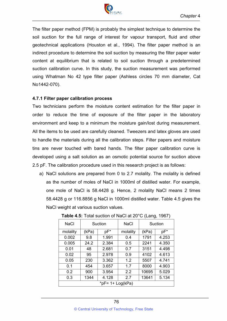
Chapter 4

76

The filter paper method (FPM) is probably the simplest technique to determine the

soil suction for the full range of interest for vapour transport, fluid and other

geotechnical applications (Houston et al., 1994). The filter paper method is an

indirect procedure to determine the soil suction by measuring the filter paper water

content at equilibrium that is related to soil suction through a predetermined

suction calibration curve. In this study, the suction measurement was performed

using Whatman No 42 type filter paper (Ashless circles 70 mm diameter, Cat

No1442-070).

4.7.1 Filter paper calibration process

Two technicians perform the moisture content estimation for the filter paper in

order to reduce the time of exposure of the filter paper in the laboratory

environment and keep to a minimum the moisture gain/lost during measurement.

All the items to be used are carefully cleaned. Tweezers and latex gloves are used

to handle the materials during all the calibration steps. Filter papers and moisture

tins are never touched with bared hands. The filter paper calibration curve is

developed using a salt solution as an osmotic potential source for suction above

2.5 pF. The calibration procedure used in this research project is as follows:

a) NaCl solutions are prepared from 0 to 2.7 molality. The molality is defined

as the number of moles of NaCl in 1000ml of distilled water. For example,

one mole of NaCl is 58.4428 g. Hence, 2 molality NaCl means 2 times

58.4428 g or 116.8856 g NaCl in 1000ml distilled water. Table 4.5 gives the

NaCl weight at various suction values.

Table 4.5: Total suction of NaCl at 20°C (Lang, 1967)

NaCl Suction NaCl Suction

molality (kPa) pF* molality (kPa) pF* 0.002 9.8 1.991 0.4 1791 4.253 0.005 24.2 2.384 0.5 2241 4.350 0.01 48 2.681 0.7 3151 4.498 0.02 95 2.978 0.9 4102 4.613 0.05 230 3.362 1.2 5507 4.741 0.1 454 3.657 1.7 8000 4.903 0.2 900 3.954 2.2 10695 5.029 0.3 1344 4.128 2.7 13641 5.134

*pF= 1+ Log(kPa)


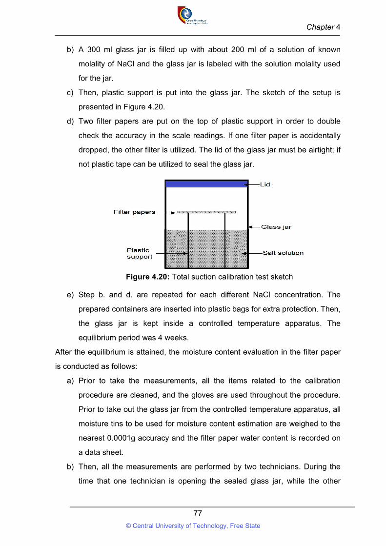
Chapter 4

77

b) A 300 ml glass jar is filled up with about 200 ml of a solution of known

molality of NaCl and the glass jar is labeled with the solution molality used

for the jar.

c) Then, plastic support is put into the glass jar. The sketch of the setup is

presented in Figure 4.20.

d) Two filter papers are put on the top of plastic support in order to double

check the accuracy in the scale readings. If one filter paper is accidentally

dropped, the other filter is utilized. The lid of the glass jar must be airtight; if

not plastic tape can be utilized to seal the glass jar.

Figure 4.20: Total suction calibration test sketch

e) Step b. and d. are repeated for each different NaCl concentration. The

prepared containers are inserted into plastic bags for extra protection. Then,

the glass jar is kept inside a controlled temperature apparatus. The

equilibrium period was 4 weeks.

After the equilibrium is attained, the moisture content evaluation in the filter paper

is conducted as follows:

a) Prior to take the measurements, all the items related to the calibration

procedure are cleaned, and the gloves are used throughout the procedure.

Prior to take out the glass jar from the controlled temperature apparatus, all

moisture tins to be used for moisture content estimation are weighed to the

nearest 0.0001g accuracy and the filter paper water content is recorded on

a data sheet.

b) Then, all the measurements are performed by two technicians. During the

time that one technician is opening the sealed glass jar, while the other


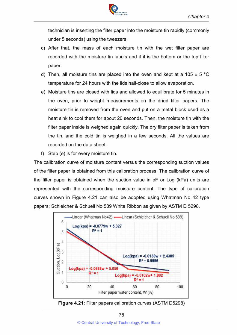
Chapter 4

78

technician is inserting the filter paper into the moisture tin rapidly (commonly

under 5 seconds) using the tweezers.

c) After that, the mass of each moisture tin with the wet filter paper are

recorded with the moisture tin labels and if it is the bottom or the top filter

paper.

d) Then, all moisture tins are placed into the oven and kept at a 105 ± 5 °C

temperature for 24 hours with the lids half-close to allow evaporation.

e) Moisture tins are closed with lids and allowed to equilibrate for 5 minutes in

the oven, prior to weight measurements on the dried filter papers. The

moisture tin is removed from the oven and put on a metal block used as a

heat sink to cool them for about 20 seconds. Then, the moisture tin with the

filter paper inside is weighed again quickly. The dry filter paper is taken from

the tin, and the cold tin is weighed in a few seconds. All the values are

recorded on the data sheet.

f) Step (e) is for every moisture tin.

The calibration curve of moisture content versus the corresponding suction values

of the filter paper is obtained from this calibration process. The calibration curve of

the filter paper is obtained when the suction value in pF or Log (kPa) units are

represented with the corresponding moisture content. The type of calibration

curves shown in Figure 4.21 can also be adopted using Whatman No 42 type

papers; Schleicher & Schuell No 589 White Ribbon as given by ASTM D 5298.

Figure 4.21: Filter papers calibration curves (ASTM D5298)


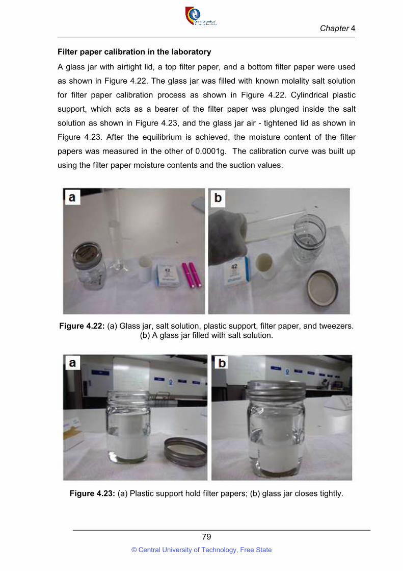
Chapter 4

79

Filter paper calibration in the laboratory

A glass jar with airtight lid, a top filter paper, and a bottom filter paper were used

as shown in Figure 4.22. The glass jar was filled with known molality salt solution

for filter paper calibration process as shown in Figure 4.22. Cylindrical plastic

support, which acts as a bearer of the filter paper was plunged inside the salt

solution as shown in Figure 4.23, and the glass jar air - tightened lid as shown in

Figure 4.23. After the equilibrium is achieved, the moisture content of the filter

papers was measured in the other of 0.0001g. The calibration curve was built up

using the filter paper moisture contents and the suction values.

Figure 4.22: (a) Glass jar, salt solution, plastic support, filter paper, and tweezers. (b) A glass jar filled with salt solution.

Figure 4.23: (a) Plastic support hold filter papers; (b) glass jar closes tightly.


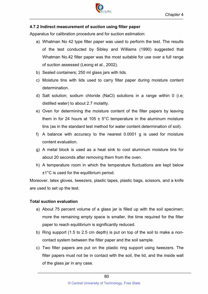
Chapter 4

80

4.7.2 Indirect measurement of suction using filter paper

Apparatus for calibration procedure and for suction estimation:

a) Whatman No 42 type filter paper was used to perform the test. The results

of the test conducted by Sibley and Williams (1990) suggested that

Whatman No.42 filter paper was the most suitable for use over a full range

of suction assessed (Leong et al., 2002).

b) Sealed containers; 250 ml glass jars with lids.

c) Moisture tins with lids used to carry filter paper during moisture content

determination.

d) Salt solution; sodium chloride (NaCl) solutions in a range within 0 (i.e;

distilled water) to about 2.7 molality.

e) Oven for determining the moisture content of the filter papers by leaving

them in for 24 hours at 105 ± 5°C temperature in the aluminum moisture

tins (as in the standard test method for water content determination of soil).

f) A balance with accuracy to the nearest 0.0001 g is used for moisture

content evaluation.

g) A metal block is used as a heat sink to cool aluminum moisture tins for

about 20 seconds after removing them from the oven.

h) A temperature room in which the temperature fluctuations are kept below

±1°C is used for the equilibrium period.

Moreover, latex gloves, tweezers, plastic tapes, plastic bags, scissors, and a knife

are used to set up the test.

Total suction evaluation

a) About 75 percent volume of a glass jar is filled up with the soil specimen;

more the remaining empty space is smaller, the time required for the filter

paper to reach equilibrium is significantly reduced.

b) Ring support (1.5 to 2.5 cm depth) is put on top of the soil to make a non-

contact system between the filter paper and the soil sample.

c) Two filter papers are put on the plastic ring support using tweezers. The

filter papers must not be in contact with the soil, the lid, and the inside wall

of the glass jar in any case.


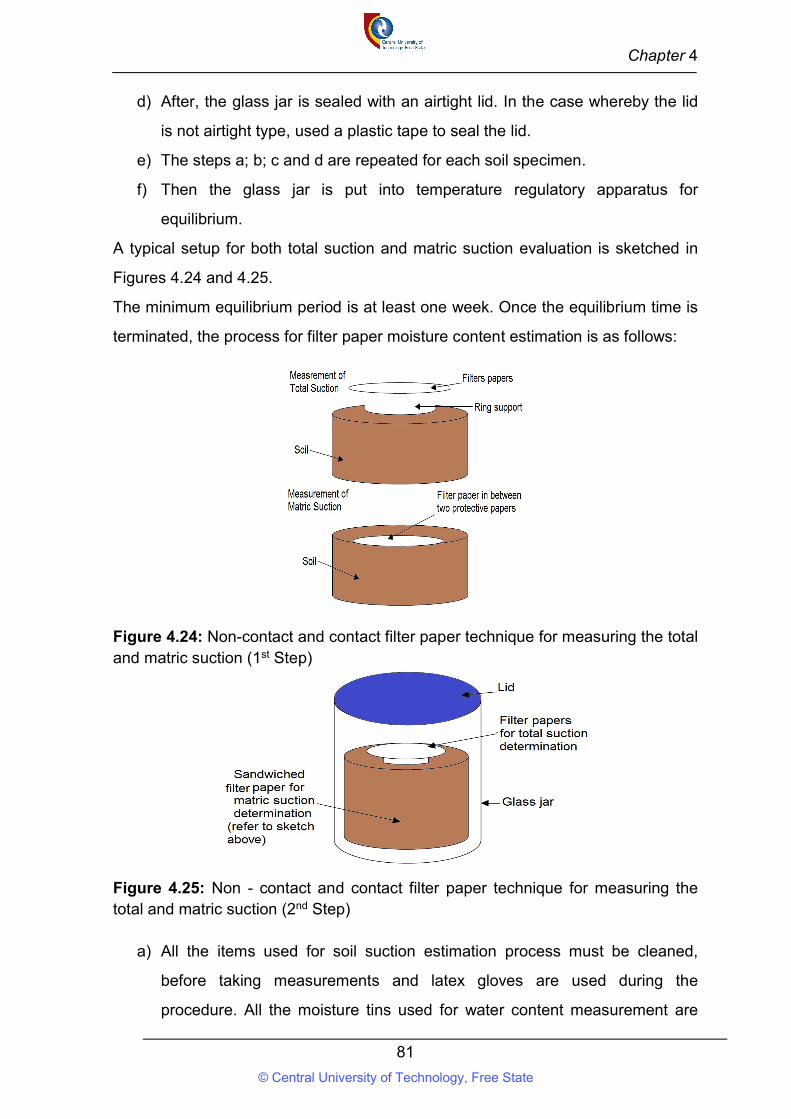
Chapter 4

81

d) After, the glass jar is sealed with an airtight lid. In the case whereby the lid

is not airtight type, used a plastic tape to seal the lid.

e) The steps a; b; c and d are repeated for each soil specimen.

f) Then the glass jar is put into temperature regulatory apparatus for

equilibrium.

A typical setup for both total suction and matric suction evaluation is sketched in

Figures 4.24 and 4.25.

The minimum equilibrium period is at least one week. Once the equilibrium time is

terminated, the process for filter paper moisture content estimation is as follows:

Figure 4.24: Non-contact and contact filter paper technique for measuring the total and matric suction (1st Step)

Figure 4.25: Non - contact and contact filter paper technique for measuring the total and matric suction (2nd Step)

a) All the items used for soil suction estimation process must be cleaned,

before taking measurements and latex gloves are used during the

procedure. All the moisture tins used for water content measurement are


Chapter 4

82

weighed to the nearest 0.0001 g precision and recorded on a data sheet,

prior to remove the glass jar from temperature regulatory apparatus.

b) Then, all estimations are performed by two technicians. For example, while

one technician is opening the sealed glass jar, the other technician is

putting the filter paper into the moisture tin rapidly (i.e. few second, usually

less than 5 seconds) by mean of tweezers.

c) After that, the mass of each moisture tins with filters paper inside is taken

rapidly. The mass of moisture tins and wet filter papers are recorded with

the corresponding moisture tin label (numbers and whether the top or

bottom filter paper is inside)

d) Step (c) is followed for every glass jar. After that, all moisture tins are put

into the oven with the lids half - close to allow evaporation. All filter papers

are kept in the oven at 105 ± 5°C temperature for 24 hours.

e) Moisture tins are closed with their lids to permit equilibrium for 5 minutes in

the oven prior to undertake the measurements on the dried filter papers.

After moisture tin is removed from the oven and put on a metal block for

about 20 seconds to cool down. Then, the moisture tin with dry filter paper

inside is weighed again quickly. The dry filter paper is taken from the can,

and the cold can be weighed within a few seconds. Lastly, all the masses

are booked on the data sheet.

f) Step (e) is repeated for every moisture tin.

Matric suction evaluation

a) The filter paper is inserted between two bigger sizes of protective filter

papers. The filter papers used in suction estimation are 70 mm diameter,

so either the filter paper is cut to a smaller diameter and inserted between

two 70 mm papers or bigger diameter ( bigger than 70 mm) filter paper are

used a protective filter paper.

b) After that, these filter papers are inserted into the soil sample, which can fill

the glass jar, in a proper contact manner. Adequate contact between the

soil specimen and the filter paper is very relevant.


Chapter 4

83

c) Then, the soil specimen with the embedded filter papers is inserted into the

glass jar container.

d) The glass jar is sealed with an airtight lid, in case the lid is not airtight one,

electrical tape can be used to seal up the lid.

e) Step a; b; c; and d. are repeated for every soil specimen.

f) The prepared glass jars are put in a temperature regulatory apparatus for

equilibrium.

Once the equilibrium period is achieved, the process of the filter paper moisture

content is conducted as follows:

a) Before starting taking measurements, all the items used for suction

measurement process are carefully cleaned and gloves are used

throughout the procedure. All moisture tins that are used for water content

determination are weighed to nearest 0.0001g accuracy before the moisture

tins are taken to the temperature regulatory apparatus, and recorded on the

measurement data sheet.

b) Then, two technicians carry out all measurements. For example, while one

technician is opening the sealed glass jar, the other technician places the

filter paper into the aluminum can be using tweezers very quickly.

c) After that, the mass of each can with the filter paper inside is taken rapidly.

The masses of wet filter paper and moisture tins are recorded with the

corresponding moisture tin number.

d) Step (c) is followed for every glass jar. All moisture tins are put inside the

oven with lids half - close to permit evaporation. All are kept at a 105 ± 5°C

temperature for 24 hours inside the oven.

e) Moisture tins are closed with their lids and permitted to equilibrate for 5

minutes in the oven, prior for undertaking the measurements on the dried

filter papers. After that, the moisture tin is removed from the oven and put

on a metal block for about 20 seconds to cool down. Then, the moisture can

with dry filter paper inside is weighed again very quickly. The dry filter paper


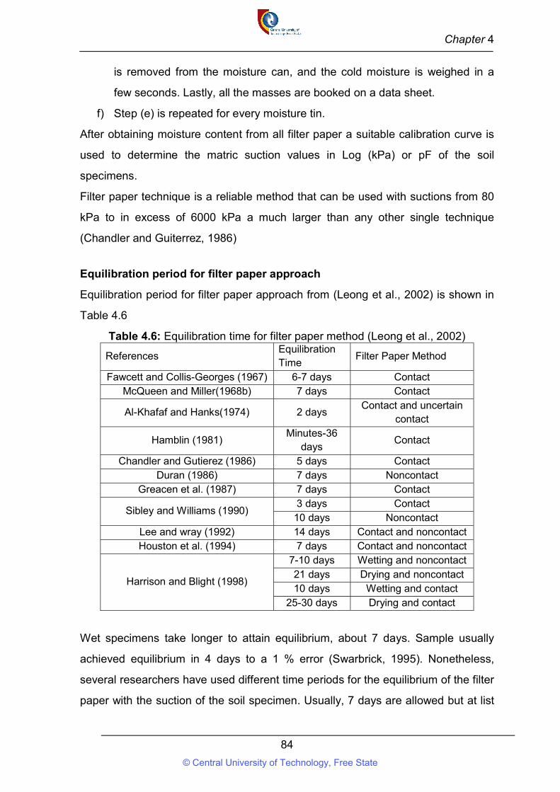
Chapter 4

84

is removed from the moisture can, and the cold moisture is weighed in a

few seconds. Lastly, all the masses are booked on a data sheet.

f) Step (e) is repeated for every moisture tin.

After obtaining moisture content from all filter paper a suitable calibration curve is

used to determine the matric suction values in Log (kPa) or pF of the soil

specimens.

Filter paper technique is a reliable method that can be used with suctions from 80

kPa to in excess of 6000 kPa a much larger than any other single technique

(Chandler and Guiterrez, 1986)

Equilibration period for filter paper approach

Equilibration period for filter paper approach from (Leong et al., 2002) is shown in

Table 4.6

Table 4.6: Equilibration time for filter paper method (Leong et al., 2002)

References Equilibration Time

Filter Paper Method

Fawcett and Collis-Georges (1967) 6-7 days Contact McQueen and Miller(1968b) 7 days Contact

Al-Khafaf and Hanks(1974) 2 days Contact and uncertain

contact

Hamblin (1981) Minutes-36

days Contact

Chandler and Gutierez (1986) 5 days Contact Duran (1986) 7 days Noncontact

Greacen et al. (1987) 7 days Contact

Sibley and Williams (1990) 3 days Contact 10 days Noncontact

Lee and wray (1992) 14 days Contact and noncontact Houston et al. (1994) 7 days Contact and noncontact

Harrison and Blight (1998)

7-10 days Wetting and noncontact 21 days Drying and noncontact 10 days Wetting and contact

25-30 days Drying and contact

Wet specimens take longer to attain equilibrium, about 7 days. Sample usually

achieved equilibrium in 4 days to a 1 % error (Swarbrick, 1995). Nonetheless,

several researchers have used different time periods for the equilibrium of the filter

paper with the suction of the soil specimen. Usually, 7 days are allowed but at list


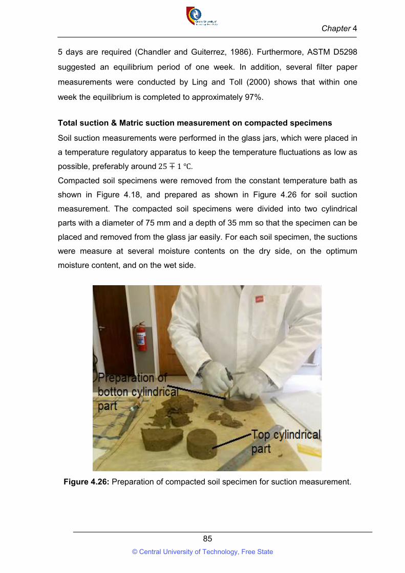
Chapter 4

85

5 days are required (Chandler and Guiterrez, 1986). Furthermore, ASTM D5298

suggested an equilibrium period of one week. In addition, several filter paper

measurements were conducted by Ling and Toll (2000) shows that within one

week the equilibrium is completed to approximately 97%.

Total suction & Matric suction measurement on compacted specimens

Soil suction measurements were performed in the glass jars, which were placed in

a temperature regulatory apparatus to keep the temperature fluctuations as low as

possible, preferably around 25 ∓ 1 ℃.

Compacted soil specimens were removed from the constant temperature bath as

shown in Figure 4.18, and prepared as shown in Figure 4.26 for soil suction

measurement. The compacted soil specimens were divided into two cylindrical

parts with a diameter of 75 mm and a depth of 35 mm so that the specimen can be

placed and removed from the glass jar easily. For each soil specimen, the suctions

were measure at several moisture contents on the dry side, on the optimum

moisture content, and on the wet side.

Figure 4.26: Preparation of compacted soil specimen for suction measurement.


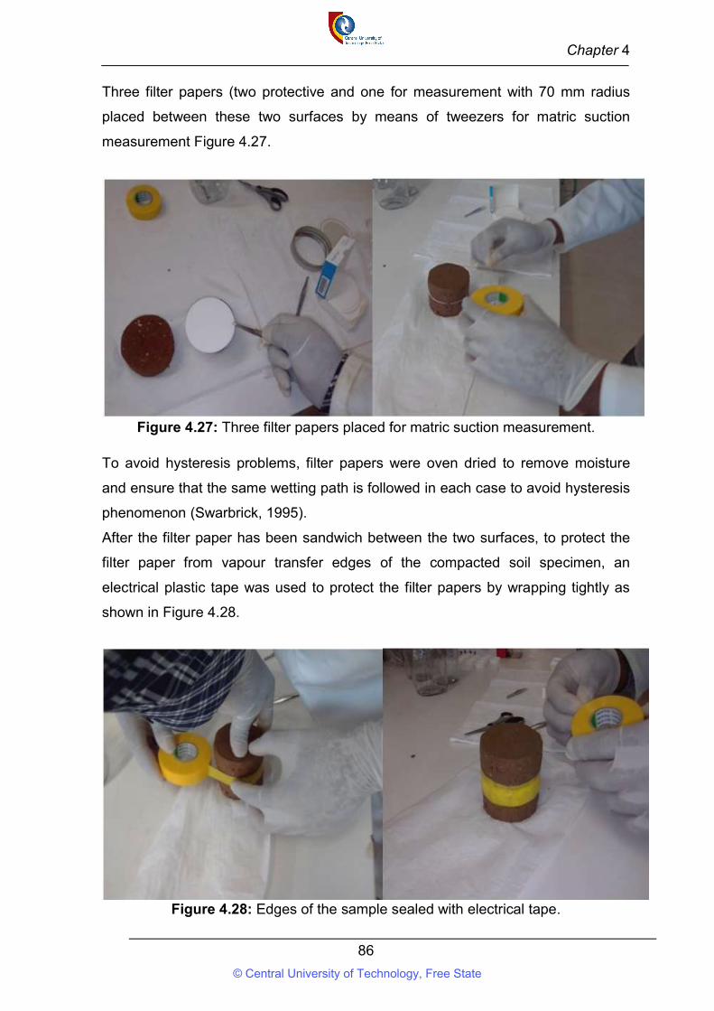
Chapter 4

86

Three filter papers (two protective and one for measurement with 70 mm radius

placed between these two surfaces by means of tweezers for matric suction

measurement Figure 4.27.

Figure 4.27: Three filter papers placed for matric suction measurement.

To avoid hysteresis problems, filter papers were oven dried to remove moisture

and ensure that the same wetting path is followed in each case to avoid hysteresis

phenomenon (Swarbrick, 1995).

After the filter paper has been sandwich between the two surfaces, to protect the

filter paper from vapour transfer edges of the compacted soil specimen, an

electrical plastic tape was used to protect the filter papers by wrapping tightly as


Figure 4.28: Edges of the sample sealed with electrical tape.


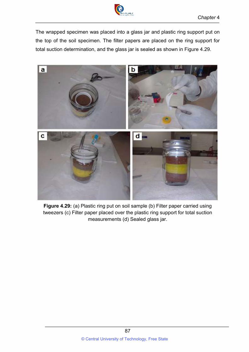
Chapter 4

87

The wrapped specimen was placed into a glass jar and plastic ring support put on

the top of the soil specimen. The filter papers are placed on the ring support for

total suction determination, and the glass jar is sealed as shown in Figure 4.29.

Figure 4.29: (a) Plastic ring put on soil sample (b) Filter paper carried using tweezers (c) Filter paper placed over the plastic ring support for total suction

measurements (d) Sealed glass jar.


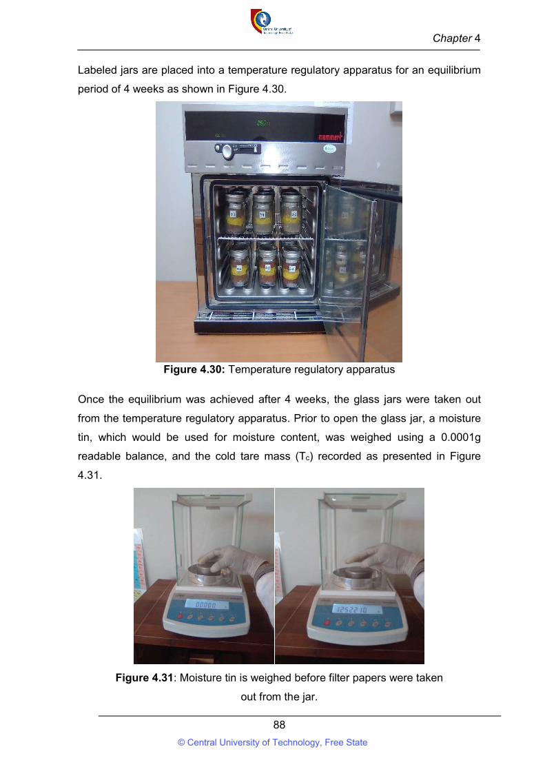
Chapter 4

88

Labeled jars are placed into a temperature regulatory apparatus for an equilibrium

period of 4 weeks as shown in Figure 4.30.

Figure 4.30: Temperature regulatory apparatus

Once the equilibrium was achieved after 4 weeks, the glass jars were taken out

from the temperature regulatory apparatus. Prior to open the glass jar, a moisture

tin, which would be used for moisture content, was weighed using a 0.0001g

readable balance, and the cold tare mass (Tc) recorded as presented in Figure

4.31.

Figure 4.31: Moisture tin is weighed before filter papers were taken

out from the jar.


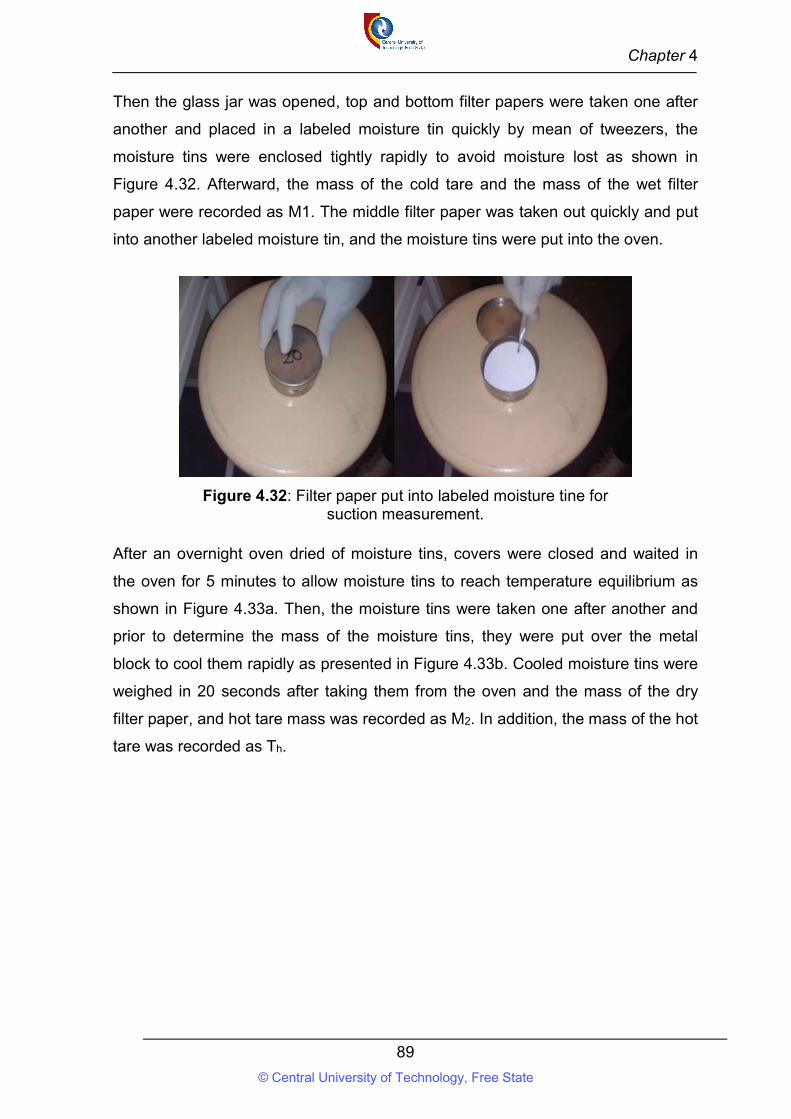
Chapter 4

89

Then the glass jar was opened, top and bottom filter papers were taken one after

another and placed in a labeled moisture tin quickly by mean of tweezers, the

moisture tins were enclosed tightly rapidly to avoid moisture lost as shown in

Figure 4.32. Afterward, the mass of the cold tare and the mass of the wet filter

paper were recorded as M1. The middle filter paper was taken out quickly and put

into another labeled moisture tin, and the moisture tins were put into the oven.

Figure 4.32: Filter paper put into labeled moisture tine for suction measurement.

After an overnight oven dried of moisture tins, covers were closed and waited in

the oven for 5 minutes to allow moisture tins to reach temperature equilibrium as

shown in Figure 4.33a. Then, the moisture tins were taken one after another and

prior to determine the mass of the moisture tins, they were put over the metal

block to cool them rapidly as presented in Figure 4.33b. Cooled moisture tins were

weighed in 20 seconds after taking them from the oven and the mass of the dry

filter paper, and hot tare mass was recorded as M2. In addition, the mass of the hot

tare was recorded as Th.


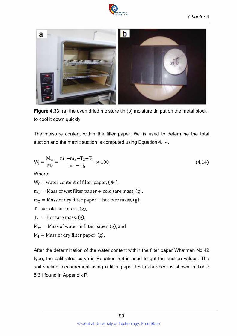
Chapter 4

90

Figure 4.33: (a) the oven dried moisture tin (b) moisture tin put on the metal block

to cool it down quickly.

The moisture content within the filter paper, Wf, is used to determine the total

suction and the matric suction is computed using Equation 4.14.

W =M

M=

m −m −T +T

m − T × 100 (4.14)

Where:

W = water content of filter paper, ( %),

m = Mass of wet filter paper + cold tare mass, (g),

m = Mass of dry filter paper + hot tare mass, (g),

T = Cold tare mass, (g),

T = Hot tare mass, (g),

M = Mass of water in filter paper, (g), and

M = Mass of dry filter paper, (g).

After the determination of the water content within the filter paper Whatman No.42

type, the calibrated curve in Equation 5.6 is used to get the suction values. The

soil suction measurement using a filter paper test data sheet is shown in Table

5.31 found in Appendix P.


Chapter 4

91

4.8 Multiple regression analyses

4.8.1 Introduction

Regression analysis is one of the most extensively used methods for analyzing

multifactor data. It is an efficient tool because it gives an easy method for

assessing functional relationships between dependent variables and an

independent variables, formulate equations or models that link the dependent

variables and one or more independent variables. Nowadays, almost all analysis

pertaining to regression analysis is performed using a software. NCSS11 software

package is intensively used in this study.

4.8.2 Regression analysis process

The regression analysis process in this study is conducted according to the

following steps:

- Formulation of the problem

- Selection of the potentially relevant variables

- Collection of the data

- Model specification

- Choice of the fitting method

- Model fitting

- Model validation

4.8.3 Statement of the problem

The question to be addressed by the multi-regression analysis is to build up

models used to predict the swelling stress of compacted expansive soils using

data collected from laboratory works. This first step is important because a poorly

formulated question can lead to the selection of an irrelevant set of variables, a

wrong choice of a model or incorrect method of analysis.

4.8.4 Selection of relevant variables

The investigation carried out in Chapter 3 section 3.4 has revealed that several soil

parameters have been used as independent variables to predict the swelling

stress. These parameters can be classified into four groups as follows:


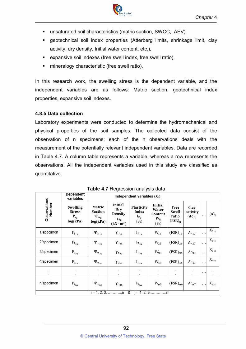
Chapter 4

92

unsaturated soil characteristics (matric suction, SWCC, AEV)

geotechnical soil index properties (Atterberg limits, shrinkage limit, clay

activity, dry density, Initial water content, etc.),

expansive soil indexes (free swell index, free swell ratio),

mineralogy characteristic (free swell ratio).

In this research work, the swelling stress is the dependent variable, and the

independent variables are as follows: Matric suction, geotechnical index

properties, expansive soil indexes.

4.8.5 Data collection

Laboratory experiments were conducted to determine the hydromechanical and

physical properties of the soil samples. The collected data consist of the

observation of n specimens; each of the n observations deals with the

measurement of the potentially relevant independent variables. Data are recorded

in Table 4.7. A column table represents a variable, whereas a row represents the

observations. All the independent variables used in this study are classified as

quantitative.

Table 4.7 Regression analysis data


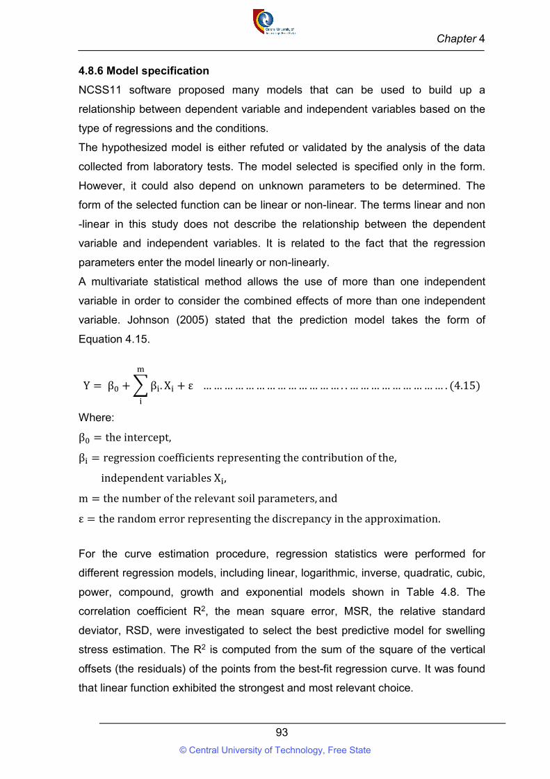
Chapter 4

93

4.8.6 Model specification

NCSS11 software proposed many models that can be used to build up a

relationship between dependent variable and independent variables based on the

type of regressions and the conditions.

The hypothesized model is either refuted or validated by the analysis of the data

collected from laboratory tests. The model selected is specified only in the form.

However, it could also depend on unknown parameters to be determined. The

form of the selected function can be linear or non-linear. The terms linear and non

-linear in this study does not describe the relationship between the dependent

variable and independent variables. It is related to the fact that the regression

parameters enter the model linearly or non-linearly.

A multivariate statistical method allows the use of more than one independent

variable in order to consider the combined effects of more than one independent

variable. Johnson (2005) stated that the prediction model takes the form of

Equation 4.15.

Y = β + β . X + ε … … … … … … … … … … … … … . . … … … … … … … … … . (4.15)

Where:

β = the intercept,

β = regression coefficients representing the contribution of the,

independent variables X ,

m = the number of the relevant soil parameters, and

ε = the random error representing the discrepancy in the approximation.

For the curve estimation procedure, regression statistics were performed for

different regression models, including linear, logarithmic, inverse, quadratic, cubic,

power, compound, growth and exponential models shown in Table 4.8. The

correlation coefficient R2, the mean square error, MSR, the relative standard

deviator, RSD, were investigated to select the best predictive model for swelling

stress estimation. The R2 is computed from the sum of the square of the vertical

offsets (the residuals) of the points from the best-fit regression curve. It was found

that linear function exhibited the strongest and most relevant choice.


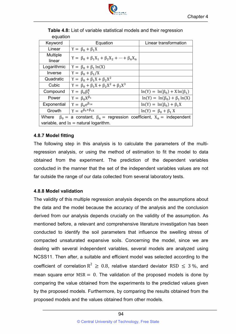
Chapter 4

94

Table 4.8: List of variable statistical models and their regression equation

Keyword Equation Linear transformation Linear Y = β + β X

Multiple linear

Y = β + β X + β X + ⋯ + β X

Logarithmic Y = β + β ln(X) Inverse Y = β + β /X

Quadratic Y = β + β X + β X

Cubic Y = β + β X + β X + β X

Compound Y = β β ln(Y) = ln(β ) + X ln(β )

Power Y = β X ln(Y) = ln(β ) + β ln(X)

Exponential Y = β e ln(Y) = ln(β ) + β X

Growth Y = e ln(Y) = β + β X

Where β = a constant, β = regression coefficient, X = independent variable, and ln = natural logarithm.

4.8.7 Model fitting

The following step in this analysis is to calculate the parameters of the multi-

regression analysis, or using the method of estimation to fit the model to data

obtained from the experiment. The prediction of the dependent variables

conducted in the manner that the set of the independent variables values are not

far outside the range of our data collected from several laboratory tests.

4.8.8 Model validation

The validity of this multiple regression analysis depends on the assumptions about

the data and the model because the accuracy of the analysis and the conclusion

derived from our analysis depends crucially on the validity of the assumption. As

mentioned before, a relevant and comprehensive literature investigation has been

conducted to identify the soil parameters that influence the swelling stress of

compacted unsaturated expansive soils. Concerning the model, since we are

dealing with several independent variables, several models are analyzed using

NCSS11. Then after, a suitable and efficient model was selected according to the

coefficient of correlation R2 ≥ 0.8, relative standard deviator RSD ≤ 3 %, and

mean square error MSR = 0. The validation of the proposed models is done by

comparing the value obtained from the experiments to the predicted values given

by the proposed models. Furthermore, by comparing the results obtained from the

proposed models and the values obtained from other models.


Chapter 4

95

In this research work, multiple regression analyses are used to diagnose, validate,

and even modify the inputs. The process is repeated until a satisfactory result is

obtained. A satisfactory output is an estimated model that satisfies the

assumptions and fits the data reasonably well.


Chapter 5

96

CHAPTER 5: ADVANCED TESTING AND ANALYSIS

5.1 Introduction

In this study, several laboratory tests which include particle size distribution,

Atterberg limits, linear shrinkage, X-ray diffraction (XRD), specific gravity, free

swell index, free swell ratio, modified Proctor compaction test, soil suction

measurement using filter paper technique, zero swelling test (ZST), and the soil

water characteristic curve (SWCC) were performed. In order to characterize the

swelling stress of compacted expansive soils, correlations between the swelling

stress and other soil parameters were established. Moreover, models to predict

the swelling stress of compacted expansive soils were developed. The laboratory

tests procedures were described in Chapter 4. In order to reduce discrepancies

and obtain reliable results, all experiments were replicated three times. As the

results were close, the average values are submitted as a final result.

In this chapter, laboratory tests results are analyzed, discussed, presented in a

form of graphs, figures, and summarized in tables.

Secondly, the analysis and discussion of correlations between swelling stress and

other soil properties such as unsaturated soil characteristics (matric suction,

SWCC), geotechnical index properties (plasticity index, liquid limit, initial water

content, initial dry density, linear shrinkage, activity of clay, clay fraction),

expansive soil characteristics (free swell index, free swell ratio).

Thirdly, predictive models to estimate the swelling stress of compacted expansive

soils were obtained from laboratory data. Models were developed by multi-

regression analysis using software NCSS11.

The validation of the proposed models is achieved by comparing the predicted

values to values obtained from experimental works. Furthermore, predicted values

are compared to results obtained from other models.

5.2 Soil characteristic properties

Standard laboratory experiments were conducted in this research to obtain the

physical and hydromechanical properties of soils.

5.2.1 Grain size classification analysis

Particle size analysis test was performed on soils WKS, WBS, BLS, PTS, and BTS

in accordance with ASTM D6913 for sieve analysis, and ATSM D7928 for


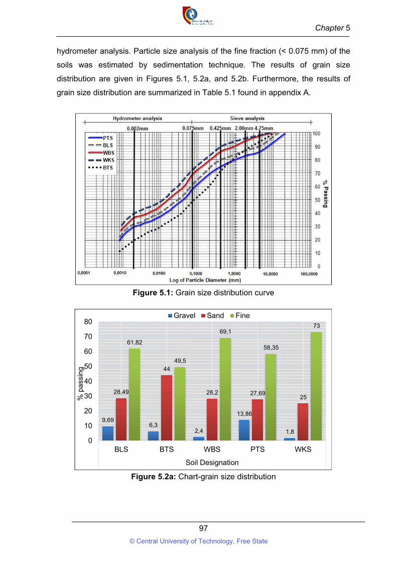
Chapter 5

97

hydrometer analysis. Particle size analysis of the fine fraction (< 0.075 mm) of the

soils was estimated by sedimentation technique. The results of grain size

distribution are given in Figures 5.1, 5.2a, and 5.2b. Furthermore, the results of

grain size distribution are summarized in Table 5.1 found in appendix A.

Figure 5.1: Grain size distribution curve

Figure 5.2a: Chart-grain size distribution

9,696,3

2,4

13,86

1,8

28,49

44

28,2 27,6925

61,82

49,5

69,1

58,35

73

0

10

20

30

40

50

60

70

80

BLS BTS WBS PTS WKS

Soil Designation

% p

assi

ng

Gravel Sand Fine


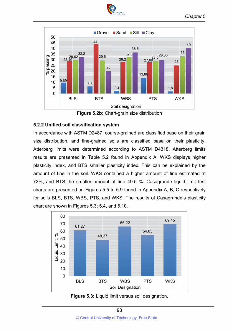
Chapter 5

98

Figure 5.2b: Chart-grain size distribution

5.2.2 Unified soil classification system

In accordance with ASTM D2487, coarse-grained are classified base on their grain

size distribution, and fine-grained soils are classified base on their plasticity.

Atterberg limits were determined according to ASTM D4318. Atterberg limits

results are presented in Table 5.2 found in Appendix A. WKS displays higher

plasticity index, and BTS smaller plasticity index. This can be explained by the

amount of fine in the soil. WKS contained a higher amount of fine estimated at

73%, and BTS the smaller amount of fine 49.5 %. Casagrande liquid limit test

charts are presented on Figures 5.5 to 5.9 found in Appendix A, B, C respectively

for soils BLS, BTS, WBS, PTS, and WKS. The results of Casagrande’s plasticity

chart are shown in Figures 5.3; 5.4, and 5.10.

Figure 5.3: Liquid limit versus soil designation.

9,696,3

2,4

13,86

1,8

28,49

44

28,2 27,69 2529,62 29,5

32,628,5

3332,2

20

36,5

29,85

40

05

101520253035404550

BLS BTS WBS PTS WKS

Soil designation

% p

assi

ng

Gravel Sand Silt Clay

61,27

48,37

66,22

54,83

69,45

0

10

20

30

40

50

60

70

80

BLS BTS WBS PTS WKS

Liq

uid

Lim

it, %

Soil Designation


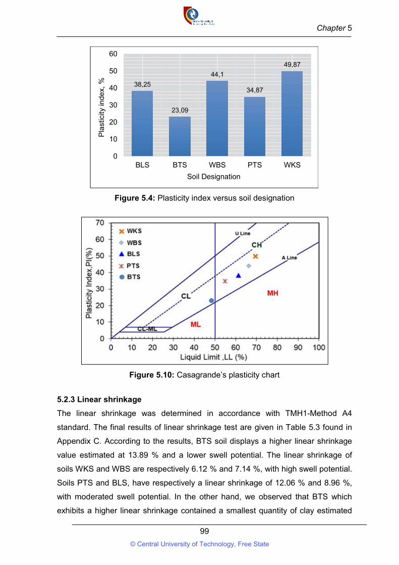
Chapter 5

99

Figure 5.4: Plasticity index versus soil designation

Figure 5.10: Casagrande’s plasticity chart

5.2.3 Linear shrinkage

The linear shrinkage was determined in accordance with TMH1-Method A4

standard. The final results of linear shrinkage test are given in Table 5.3 found in

Appendix C. According to the results, BTS soil displays a higher linear shrinkage

value estimated at 13.89 % and a lower swell potential. The linear shrinkage of

soils WKS and WBS are respectively 6.12 % and 7.14 %, with high swell potential.

Soils PTS and BLS, have respectively a linear shrinkage of 12.06 % and 8.96 %,

with moderated swell potential. In the other hand, we observed that BTS which

exhibits a higher linear shrinkage contained a smallest quantity of clay estimated

38,25

23,09

44,1

34,87

49,87

0

10

20

30

40

50

60

BLS BTS WBS PTS WKS

Pla

stic

ity in

dex,

%

Soil Designation


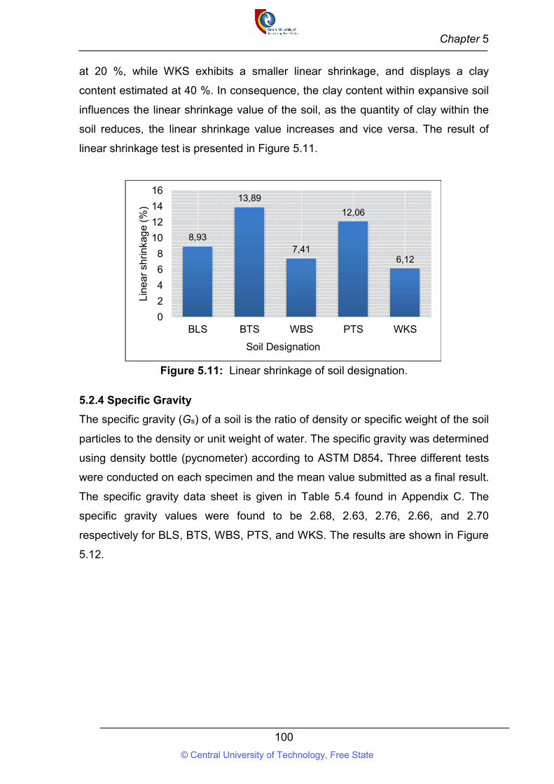
Chapter 5

100

at 20 %, while WKS exhibits a smaller linear shrinkage, and displays a clay

content estimated at 40 %. In consequence, the clay content within expansive soil

influences the linear shrinkage value of the soil, as the quantity of clay within the

soil reduces, the linear shrinkage value increases and vice versa. The result of

linear shrinkage test is presented in Figure 5.11.

Figure 5.11: Linear shrinkage of soil designation.

5.2.4 Specific Gravity

The specific gravity (Gs) of a soil is the ratio of density or specific weight of the soil

particles to the density or unit weight of water. The specific gravity was determined

using density bottle (pycnometer) according to ASTM D854. Three different tests

were conducted on each specimen and the mean value submitted as a final result.

The specific gravity data sheet is given in Table 5.4 found in Appendix C. The

specific gravity values were found to be 2.68, 2.63, 2.76, 2.66, and 2.70

respectively for BLS, BTS, WBS, PTS, and WKS. The results are shown in Figure

5.12.

8,93

13,89

7,41

12,06

6,12

0

2

4

6

8

10

12

14

16

BLS BTS WBS PTS WKS

Lin

ear

shrin

kag

e (%

)

Soil Designation


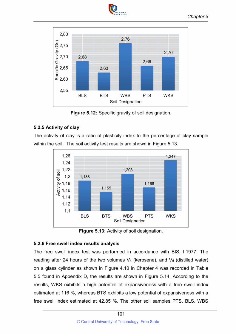
Chapter 5

101

Figure 5.12: Specific gravity of soil designation.

5.2.5 Activity of clay

The activity of clay is a ratio of plasticity index to the percentage of clay sample

within the soil. The soil activity test results are shown in Figure 5.13.

Figure 5.13: Activity of soil designation.

5.2.6 Free swell index results analysis

The free swell index test was performed in accordance with BIS, I.1977. The

reading after 24 hours of the two volumes Vk (kerosene), and Vd (distilled water)

on a glass cylinder as shown in Figure 4.10 in Chapter 4 was recorded in Table

5.5 found in Appendix D, the results are shown in Figure 5.14. According to the

results, WKS exhibits a high potential of expansiveness with a free swell index

estimated at 116 %, whereas BTS exhibits a low potential of expansiveness with a

free swell index estimated at 42.85 %. The other soil samples PTS, BLS, WBS

2,68

2,63

2,76

2,66

2,70

2,55

2,60

2,65

2,70

2,75

2,80

BLS BTS WBS PTS WKS

Sp

ecifi

c G

ravi

ty (

Gs)

Soil Designation

1,188

1,155

1,208

1,168

1,247

1,1

1,12

1,14

1,16

1,18

1,2

1,22

1,24

1,26

BLS BTS WBS PTS WKS

Act

ivity

of s

oil

Soil Designation


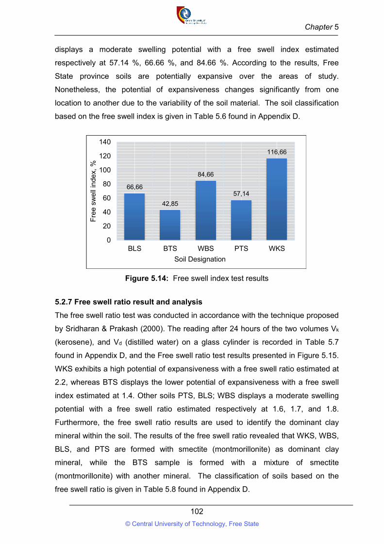
Chapter 5

102

displays a moderate swelling potential with a free swell index estimated

respectively at 57.14 %, 66.66 %, and 84.66 %. According to the results, Free

State province soils are potentially expansive over the areas of study.

Nonetheless, the potential of expansiveness changes significantly from one

location to another due to the variability of the soil material. The soil classification

based on the free swell index is given in Table 5.6 found in Appendix D.

Figure 5.14: Free swell index test results

5.2.7 Free swell ratio result and analysis

The free swell ratio test was conducted in accordance with the technique proposed

by Sridharan & Prakash (2000). The reading after 24 hours of the two volumes Vk

(kerosene), and Vd (distilled water) on a glass cylinder is recorded in Table 5.7

found in Appendix D, and the Free swell ratio test results presented in Figure 5.15.

WKS exhibits a high potential of expansiveness with a free swell ratio estimated at

2.2, whereas BTS displays the lower potential of expansiveness with a free swell

index estimated at 1.4. Other soils PTS, BLS; WBS displays a moderate swelling

potential with a free swell ratio estimated respectively at 1.6, 1.7, and 1.8.

Furthermore, the free swell ratio results are used to identify the dominant clay

mineral within the soil. The results of the free swell ratio revealed that WKS, WBS,

BLS, and PTS are formed with smectite (montmorillonite) as dominant clay

mineral, while the BTS sample is formed with a mixture of smectite

(montmorillonite) with another mineral. The classification of soils based on the

free swell ratio is given in Table 5.8 found in Appendix D.

66,66

42,85

84,66

57,14

116,66

0

20

40

60

80

100

120

140

BLS BTS WBS PTS WKS

Fre

e sw

ell

inde

x, %

Soil Designation


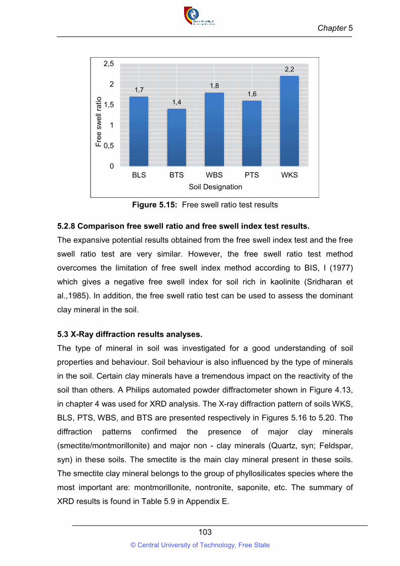
Chapter 5

103

Figure 5.15: Free swell ratio test results

5.2.8 Comparison free swell ratio and free swell index test results.

The expansive potential results obtained from the free swell index test and the free

swell ratio test are very similar. However, the free swell ratio test method

overcomes the limitation of free swell index method according to BIS, I (1977)

which gives a negative free swell index for soil rich in kaolinite (Sridharan et

al.,1985). In addition, the free swell ratio test can be used to assess the dominant

clay mineral in the soil.

5.3 X-Ray diffraction results analyses.

The type of mineral in soil was investigated for a good understanding of soil

properties and behaviour. Soil behaviour is also influenced by the type of minerals

in the soil. Certain clay minerals have a tremendous impact on the reactivity of the

soil than others. A Philips automated powder diffractometer shown in Figure 4.13,

in chapter 4 was used for XRD analysis. The X-ray diffraction pattern of soils WKS,

BLS, PTS, WBS, and BTS are presented respectively in Figures 5.16 to 5.20. The

diffraction patterns confirmed the presence of major clay minerals

(smectite/montmorillonite) and major non - clay minerals (Quartz, syn; Feldspar,

syn) in these soils. The smectite is the main clay mineral present in these soils.

The smectite clay mineral belongs to the group of phyllosilicates species where the

most important are: montmorillonite, nontronite, saponite, etc. The summary of

XRD results is found in Table 5.9 in Appendix E.

1,7

1,4

1,81,6

2,2

0

0,5

1

1,5

2

2,5

BLS BTS WBS PTS WKS

Fre

e sw

ell

ratio

Soil Designation


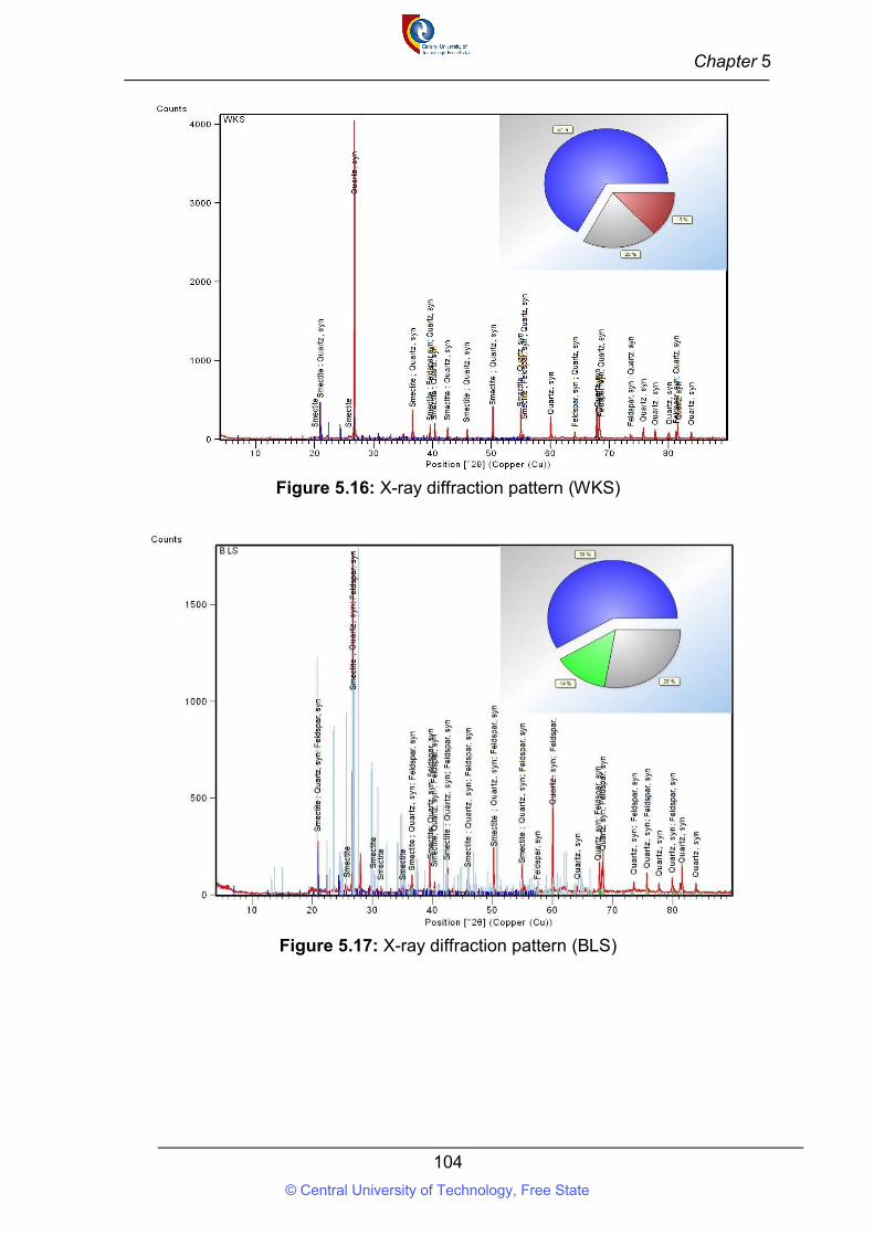
Chapter 5

104

Figure 5.16: X-ray diffraction pattern (WKS)

Figure 5.17: X-ray diffraction pattern (BLS)


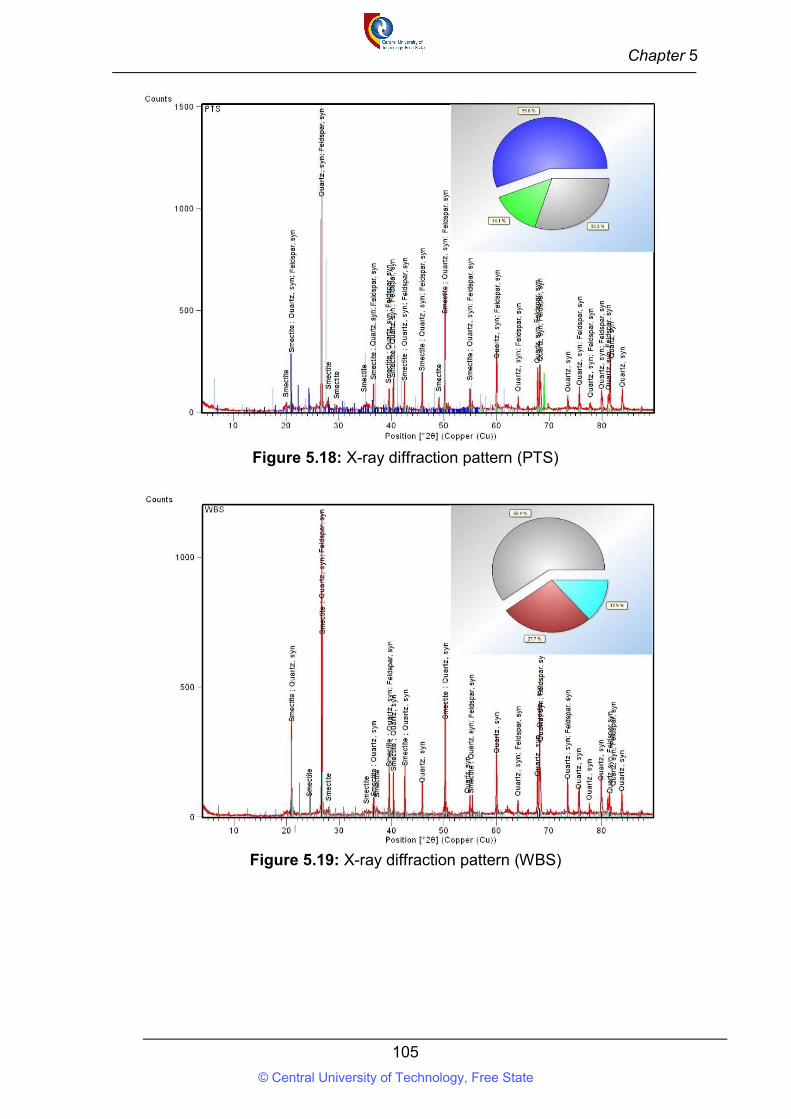
Chapter 5

105

Figure 5.18: X-ray diffraction pattern (PTS)

Figure 5.19: X-ray diffraction pattern (WBS)


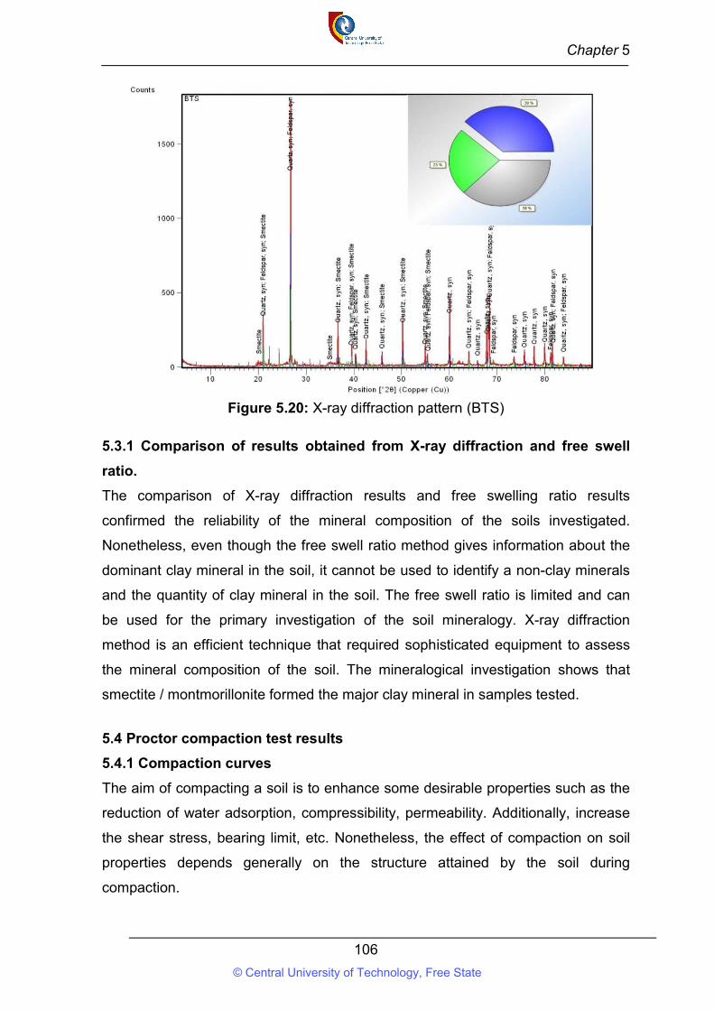
Chapter 5

106

Figure 5.20: X-ray diffraction pattern (BTS)

5.3.1 Comparison of results obtained from X-ray diffraction and free swell

ratio.

The comparison of X-ray diffraction results and free swelling ratio results

confirmed the reliability of the mineral composition of the soils investigated.

Nonetheless, even though the free swell ratio method gives information about the

dominant clay mineral in the soil, it cannot be used to identify a non-clay minerals

and the quantity of clay mineral in the soil. The free swell ratio is limited and can

be used for the primary investigation of the soil mineralogy. X-ray diffraction

method is an efficient technique that required sophisticated equipment to assess

the mineral composition of the soil. The mineralogical investigation shows that

smectite / montmorillonite formed the major clay mineral in samples tested.

5.4 Proctor compaction test results

5.4.1 Compaction curves

The aim of compacting a soil is to enhance some desirable properties such as the

reduction of water adsorption, compressibility, permeability. Additionally, increase

the shear stress, bearing limit, etc. Nonetheless, the effect of compaction on soil

properties depends generally on the structure attained by the soil during

compaction.


Chapter 5

107

The proctor compaction test was conducted according to TMH1-Method A7. The

compaction curves were plotted by preparing the soil samples at different moisture

content on the dry side at the optimum moisture content, and on the wet side. The

dry density of each soil type was obtained on the dry side, optimum moisture

content and on the wet side. The compaction curves for soils BTS, PTS, BLS,

WBS, and WKS are shown in Figure 5.21. The compaction curves and zero air

void line curves are plotted for each soil designation as shown in Figures 5.22 to

5.26. The determination of the maximum dry density and the optimum moisture

content for each soil sample were done mathematically. The interpretation of the

compaction curves revealed that BTS exhibits a higher maximum dry density

18.76 kN/m3, and WKS displays the smaller maximum dry density of 16.29 kN/m3.

The maximum dry density for soil samples PTS, BLS, and WBS are respectively

17.99 kN/m3, 17.16 kN/m3 and 16.29 kN/m3. Soil BTS which exhibits the highest

maximum dry density, contained the smallest fine fraction 49.5%, whereas WKS

which displays the smallest dry density, contained the highest fine fraction 73%.

As the fine fraction material in the soil increases, the maximum dry density

reduces upon the same compacting energy. Hence, the fine fraction materials in

expansive soil influence significantly the maximum dry density.

WKS exhibits the highest optimum water content estimated at 26.34 %, while BTS

displays the smallest optimum water content at 18.24 %. The optimum water

content for soils WBS, BLS, and PTS are respectively 24.58 %, 22.61 %, and

20.38 %. WKS which exhibits the highest optimum water content, contained the

highest fine fraction 73 %, whereas BTS, which displays the smallest optimum

moisture content, contained the smallest fine fraction 49.5 %. As the fine fraction

material in the soil increases, the optimum moisture content increases upon the

same compacting energy. Therefore, the fine fraction materials in an expansive

soils influence the optimum moisture content. The proctor compaction test results

are given in Table 5.10 found in Appendix E.


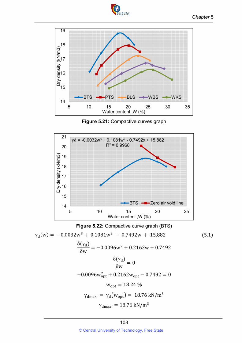
Chapter 5

108

Figure 5.21: Compactive curves graph

Figure 5.22: Compactive curve graph (BTS)

γ (w) = −0.0032w + 0.1081w − 0.7492w + 15.882 (5.1)

δ(γ )

δw= −0.0096w + 0.2162w − 0.7492

δ(γ )

δw= 0

−0.0096w + 0.2162w − 0.7492 = 0

w = 18.24 %

γ = γ w = 18.76 kN/m

γ = 18.76 kN/m

14

15

16

17

18

19

5 10 15 20 25 30 35

Dry

de

nsity

(kN

/m3)

Water content ,W (%)

BTS PTS BLS WBS WKS

γd = -0.0032w3 + 0.1081w2 - 0.7492x + 15.882R² = 0.9968

14

15

16

17

18

19

20

21

5 10 15 20 25

Dry

de

nsity

(kN

/m3)


BTS Zero air void line


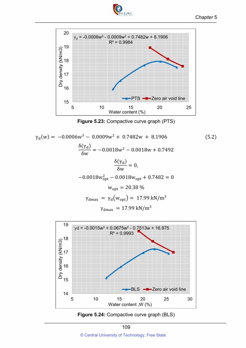
Chapter 5

109

Figure 5.23: Compactive curve graph (PTS)

γ (w) = −0.0006w − 0.0009w + 0.7482w + 8.1906 (5.2)

δ(γ )

δw= −0.0018w − 0.0018w + 0.7492

δ(γ )

δw= 0,

−0.0018w − 0.0018w + 0.7482 = 0

w = 20.38 %

γ = γ w = 17.99 kN/m

γ = 17.99 kN/m

Figure 5.24: Compactive curve graph (BLS)

γd = -0.0006w3 - 0.0009w2 + 0.7482w + 8.1906R² = 0.9984

15

16

17

18

19

20

5 10 15 20 25

Dry

de

nsity

(kN

/m3)

Water content (%)

PTS Zero air void line

γd = -0.0015w3 + 0.0675w2 - 0.7513w + 16.975R² = 0.9993

14

15

16

17

18

19

5 10 15 20 25 30

Dry

den

sity

(kN

/m3)


BLS Zero air void line


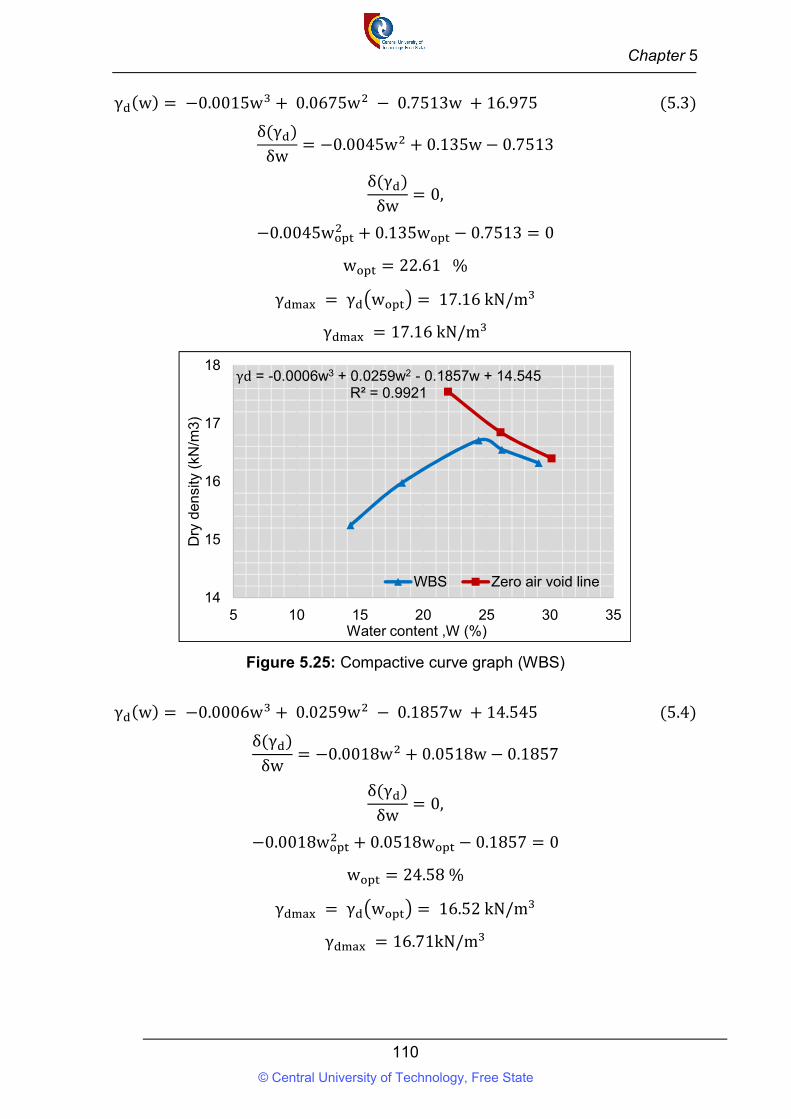
Chapter 5

110

γ (w) = −0.0015w + 0.0675w − 0.7513w + 16.975 (5.3)

δ(γ )

δw= −0.0045w + 0.135w − 0.7513

δ(γ )

δw= 0,

−0.0045w + 0.135w − 0.7513 = 0

w = 22.61 %

γ = γ w = 17.16 kN/m

γ = 17.16 kN/m

Figure 5.25: Compactive curve graph (WBS)

γ (w) = −0.0006w + 0.0259w − 0.1857w + 14.545 (5.4)

δ(γ )

δw= −0.0018w + 0.0518w − 0.1857

δ(γ )

δw= 0,

−0.0018w + 0.0518w − 0.1857 = 0

w = 24.58 %

γ = γ w = 16.52 kN/m

γ = 16.71kN/m

γd = -0.0006w3 + 0.0259w2 - 0.1857w + 14.545R² = 0.9921

14

15

16

17

18

5 10 15 20 25 30 35

Dry

den

sity

(kN

/m3)


WBS Zero air void line


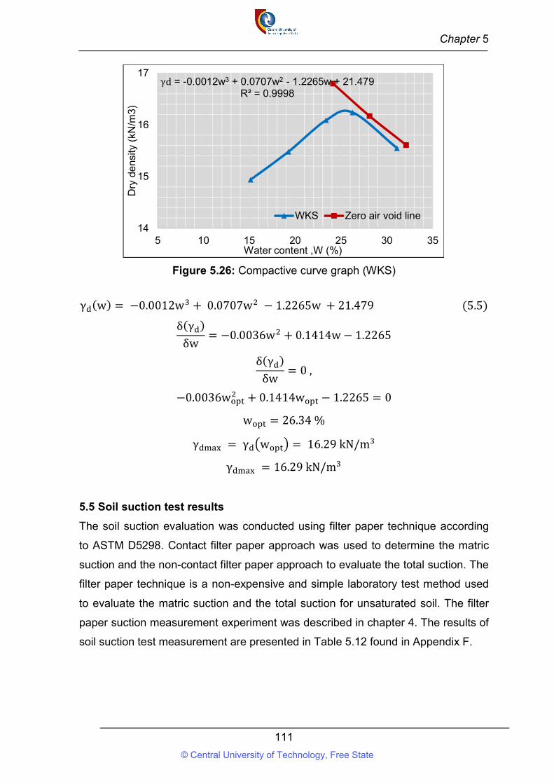
Chapter 5

111

Figure 5.26: Compactive curve graph (WKS)

γ (w) = −0.0012w + 0.0707w − 1.2265w + 21.479 (5.5)

δ(γ )

δw= −0.0036w + 0.1414w − 1.2265

δ(γ )

δw= 0 ,

−0.0036w + 0.1414w − 1.2265 = 0

w = 26.34 %

γ = γ w = 16.29 kN/m

γ = 16.29 kN/m

5.5 Soil suction test results

The soil suction evaluation was conducted using filter paper technique according

to ASTM D5298. Contact filter paper approach was used to determine the matric

suction and the non-contact filter paper approach to evaluate the total suction. The

filter paper technique is a non-expensive and simple laboratory test method used

to evaluate the matric suction and the total suction for unsaturated soil. The filter

paper suction measurement experiment was described in chapter 4. The results of

soil suction test measurement are presented in Table 5.12 found in Appendix F.

γd = -0.0012w3 + 0.0707w2 - 1.2265w + 21.479R² = 0.9998

14

15

16

17

5 10 15 20 25 30 35

Dry

de

nsity

(kN

/m3)


WKS Zero air void line


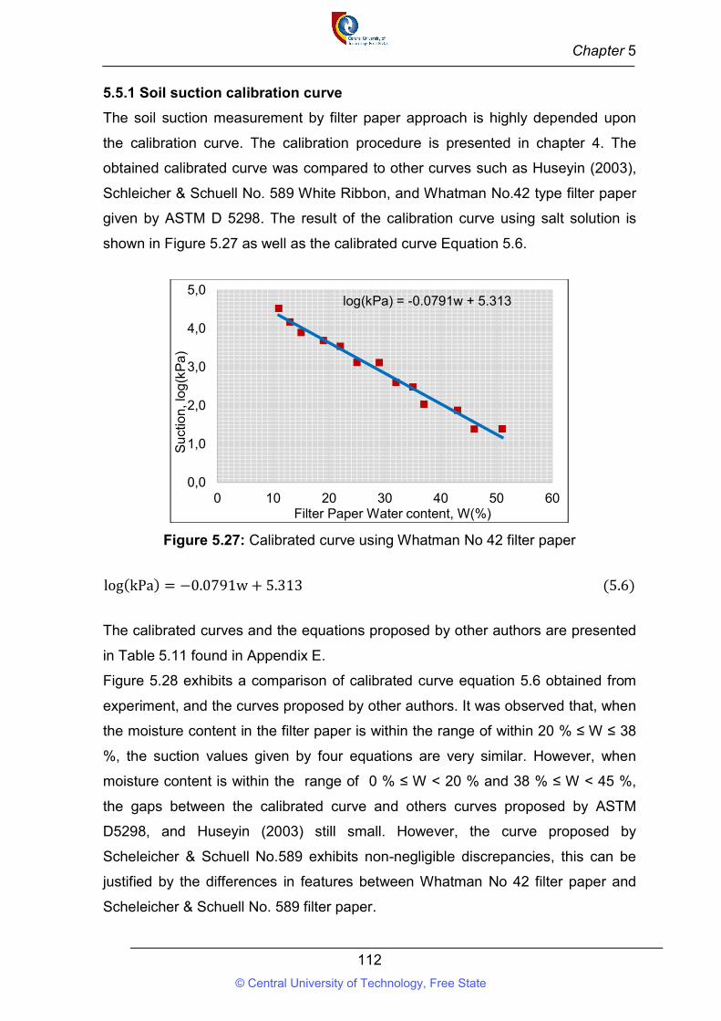
Chapter 5

112

5.5.1 Soil suction calibration curve

The soil suction measurement by filter paper approach is highly depended upon

the calibration curve. The calibration procedure is presented in chapter 4. The

obtained calibrated curve was compared to other curves such as Huseyin (2003),

Schleicher & Schuell No. 589 White Ribbon, and Whatman No.42 type filter paper

given by ASTM D 5298. The result of the calibration curve using salt solution is

shown in Figure 5.27 as well as the calibrated curve Equation 5.6.

Figure 5.27: Calibrated curve using Whatman No 42 filter paper

log(kPa) = −0.0791w + 5.313 (5.6)

The calibrated curves and the equations proposed by other authors are presented

in Table 5.11 found in Appendix E.

Figure 5.28 exhibits a comparison of calibrated curve equation 5.6 obtained from

experiment, and the curves proposed by other authors. It was observed that, when

the moisture content in the filter paper is within the range of within 20 % ≤ W ≤ 38

%, the suction values given by four equations are very similar. However, when

moisture content is within the range of 0 % ≤ W < 20 % and 38 % ≤ W < 45 %,

the gaps between the calibrated curve and others curves proposed by ASTM

D5298, and Huseyin (2003) still small. However, the curve proposed by

Scheleicher & Schuell No.589 exhibits non-negligible discrepancies, this can be

justified by the differences in features between Whatman No 42 filter paper and

Scheleicher & Schuell No. 589 filter paper.

log(kPa) = -0.0791w + 5.313

0,0

1,0

2,0

3,0

4,0

5,0

0 10 20 30 40 50 60

Su

ctio

n, l

og(k

Pa)

Filter Paper Water content, W(%)


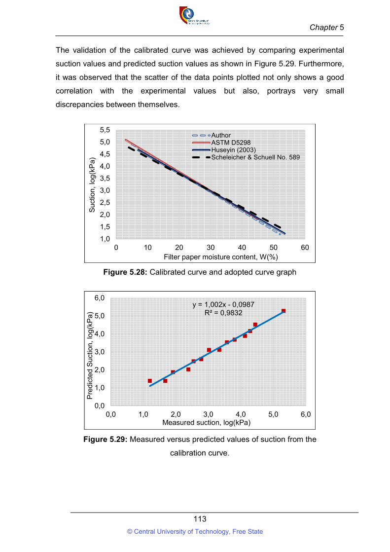
Chapter 5

113

The validation of the calibrated curve was achieved by comparing experimental

suction values and predicted suction values as shown in Figure 5.29. Furthermore,

it was observed that the scatter of the data points plotted not only shows a good

correlation with the experimental values but also, portrays very small

discrepancies between themselves.

Figure 5.28: Calibrated curve and adopted curve graph

Figure 5.29: Measured versus predicted values of suction from the

calibration curve.

1,0

1,5

2,0

2,5

3,0

3,5

4,0

4,5

5,0

5,5

0 10 20 30 40 50 60

Su

ctio

n, l

og(k

Pa)

Filter paper moisture content, W(%)

AuthorASTM D5298Huseyin (2003)Scheleicher & Schuell No. 589

y = 1,002x - 0,0987R² = 0,9832

0,0

1,0

2,0

3,0

4,0

5,0

6,0

0,0 1,0 2,0 3,0 4,0 5,0 6,0

Pre

dic

ted

Su

ctio

n, l

og(k

Pa)

Measured suction, log(kPa)


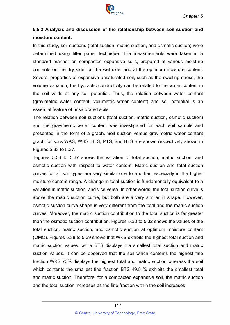
Chapter 5

114

5.5.2 Analysis and discussion of the relationship between soil suction and

moisture content.

In this study, soil suctions (total suction, matric suction, and osmotic suction) were

determined using filter paper technique. The measurements were taken in a

standard manner on compacted expansive soils, prepared at various moisture

contents on the dry side, on the wet side, and at the optimum moisture content.

Several properties of expansive unsaturated soil, such as the swelling stress, the

volume variation, the hydraulic conductivity can be related to the water content in

the soil voids at any soil potential. Thus, the relation between water content

(gravimetric water content, volumetric water content) and soil potential is an

essential feature of unsaturated soils.

The relation between soil suctions (total suction, matric suction, osmotic suction)

and the gravimetric water content was investigated for each soil sample and

presented in the form of a graph. Soil suction versus gravimetric water content

graph for soils WKS, WBS, BLS, PTS, and BTS are shown respectively shown in

Figures 5.33 to 5.37.

Figures 5.33 to 5.37 shows the variation of total suction, matric suction, and

osmotic suction with respect to water content. Matric suction and total suction

curves for all soil types are very similar one to another, especially in the higher

moisture content range. A change in total suction is fundamentally equivalent to a

variation in matric suction, and vice versa. In other words, the total suction curve is

above the matric suction curve, but both are a very similar in shape. However,

osmotic suction curve shape is very different from the total and the matric suction

curves. Moreover, the matric suction contribution to the total suction is far greater

than the osmotic suction contribution. Figures 5.30 to 5.32 shows the values of the

total suction, matric suction, and osmotic suction at optimum moisture content

(OMC). Figures 5.38 to 5.39 shows that WKS exhibits the highest total suction and

matric suction values, while BTS displays the smallest total suction and matric

suction values. It can be observed that the soil which contents the highest fine

fraction WKS 73% displays the highest total and matric suction whereas the soil

which contents the smallest fine fraction BTS 49.5 % exhibits the smallest total

and matric suction. Therefore, for a compacted expansive soil, the matric suction

and the total suction increases as the fine fraction within the soil increases.


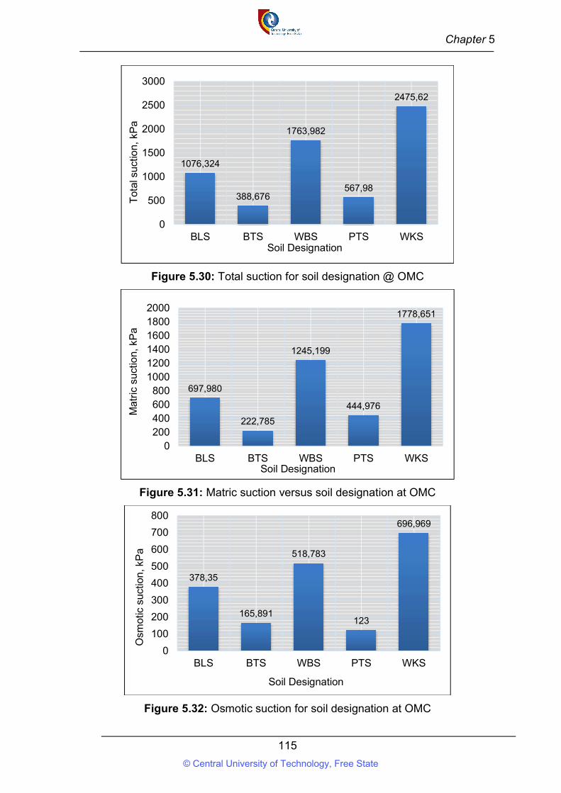
Chapter 5

115

Figure 5.30: Total suction for soil designation @ OMC

Figure 5.31: Matric suction versus soil designation at OMC

Figure 5.32: Osmotic suction for soil designation at OMC

1076,324

388,676

1763,982

567,98

2475,62

0

500

1000

1500

2000

2500

3000

BLS BTS WBS PTS WKS

Tot

al s

uctio

n, k

Pa

Soil Designation

697,980

222,785

1245,199

444,976

1778,651

0200400600800

100012001400160018002000

BLS BTS WBS PTS WKS

Mat

ric

suct

ion,

kP

a

Soil Designation

378,35

165,891

518,783

123

696,969

0

100

200

300

400

500

600

700

800

BLS BTS WBS PTS WKS

Osm

otic

suc

tion

, kP

a

Soil Designation


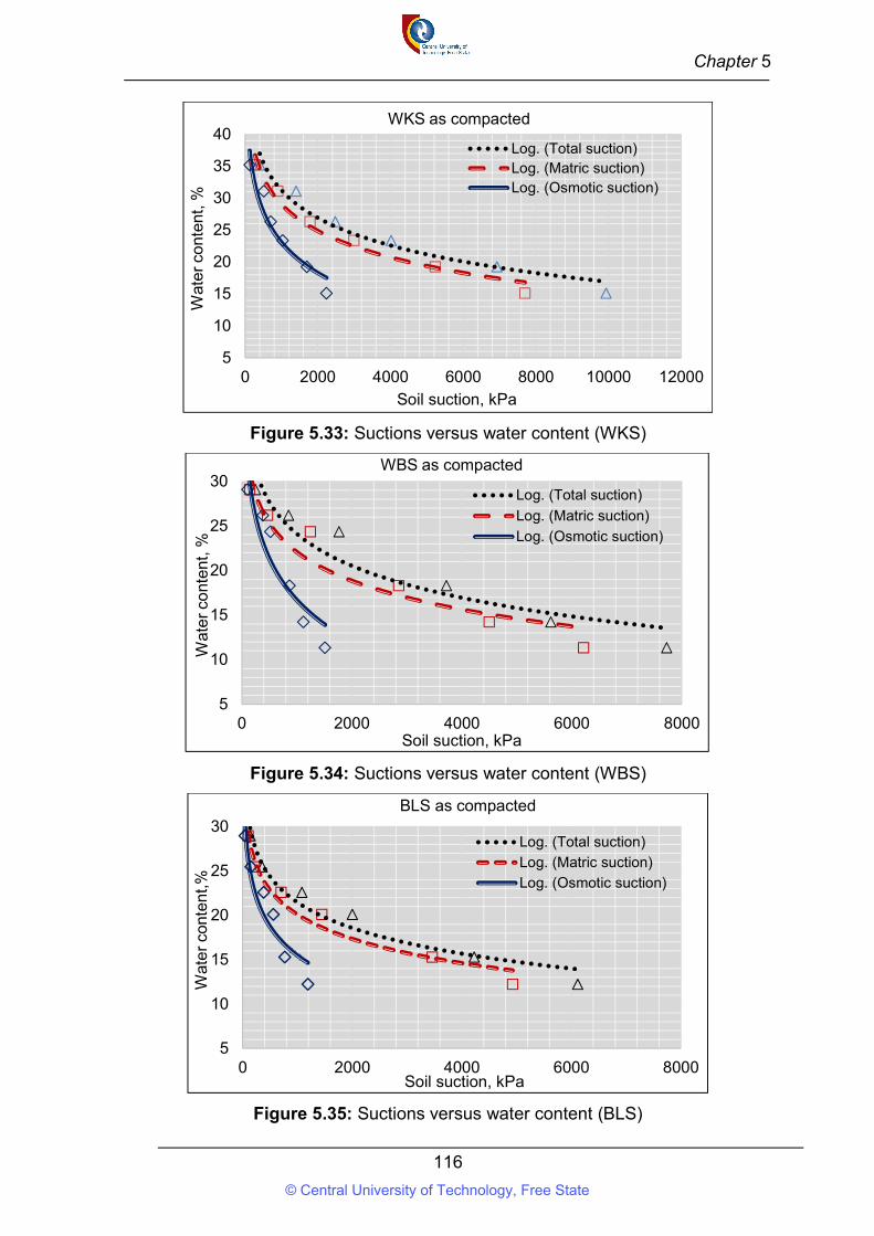
Chapter 5

116

Figure 5.33: Suctions versus water content (WKS)

Figure 5.34: Suctions versus water content (WBS)

Figure 5.35: Suctions versus water content (BLS)

5

10

15

20

25

30

35

40

0 2000 4000 6000 8000 10000 12000

Wat

er

cont

ent,

%

Soil suction, kPa

WKS as compacted

Log. (Total suction)Log. (Matric suction)Log. (Osmotic suction)

5

10

15

20

25

30

0 2000 4000 6000 8000

Wat

er

cont

ent,

%

Soil suction, kPa

WBS as compacted

Log. (Total suction)

Log. (Matric suction)

Log. (Osmotic suction)

5

10

15

20

25

30

0 2000 4000 6000 8000

Wat

er

cont

ent,

%

Soil suction, kPa

BLS as compacted

Log. (Total suction)

Log. (Matric suction)

Log. (Osmotic suction)


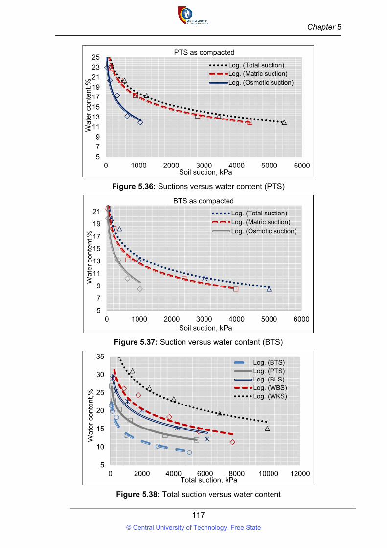
Chapter 5

117

Figure 5.36: Suctions versus water content (PTS)

Figure 5.37: Suction versus water content (BTS)

Figure 5.38: Total suction versus water content

579

1113151719212325

0 1000 2000 3000 4000 5000 6000

Wat

er

cont

ent,

%

Soil suction, kPa

PTS as compacted


5

7

9

11

13

15

17

19

21

0 1000 2000 3000 4000 5000 6000

Wat

er

cont

ent,

%

Soil suction, kPa

BTS as compacted


5

10

15

20

25

30

35

0 2000 4000 6000 8000 10000 12000

Wat

er

cont

ent,

%

Total suction, kPa

Log. (BTS)Log. (PTS)Log. (BLS)Log. (WBS)Log. (WKS)


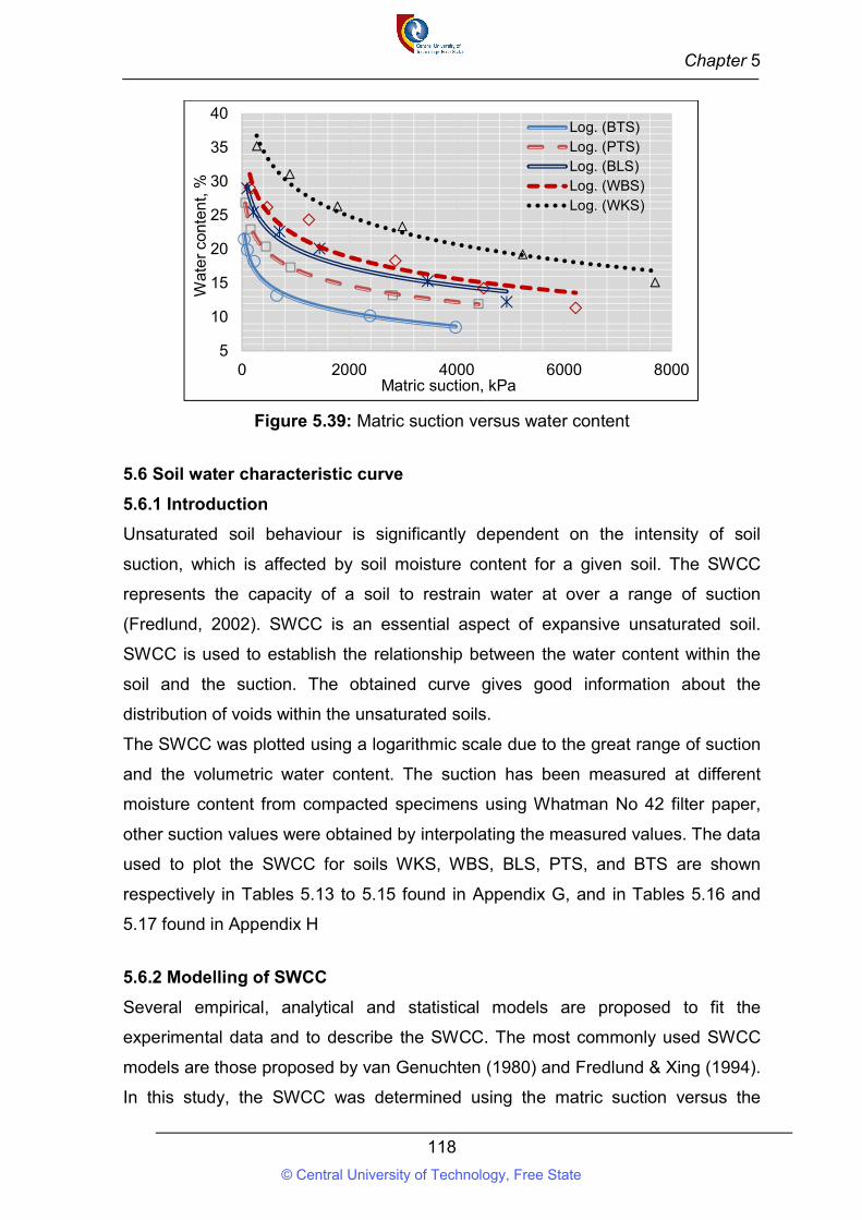
Chapter 5

118

Figure 5.39: Matric suction versus water content

5.6 Soil water characteristic curve

5.6.1 Introduction

Unsaturated soil behaviour is significantly dependent on the intensity of soil

suction, which is affected by soil moisture content for a given soil. The SWCC

represents the capacity of a soil to restrain water at over a range of suction

(Fredlund, 2002). SWCC is an essential aspect of expansive unsaturated soil.

SWCC is used to establish the relationship between the water content within the

soil and the suction. The obtained curve gives good information about the

distribution of voids within the unsaturated soils.

The SWCC was plotted using a logarithmic scale due to the great range of suction

and the volumetric water content. The suction has been measured at different

moisture content from compacted specimens using Whatman No 42 filter paper,

other suction values were obtained by interpolating the measured values. The data

used to plot the SWCC for soils WKS, WBS, BLS, PTS, and BTS are shown

respectively in Tables 5.13 to 5.15 found in Appendix G, and in Tables 5.16 and

5.17 found in Appendix H

5.6.2 Modelling of SWCC

Several empirical, analytical and statistical models are proposed to fit the

experimental data and to describe the SWCC. The most commonly used SWCC

models are those proposed by van Genuchten (1980) and Fredlund & Xing (1994).

In this study, the SWCC was determined using the matric suction versus the

5

10

15

20

25

30

35

40

0 2000 4000 6000 8000

Wat

er

cont

ent,

%

Matric suction, kPa

Log. (BTS)Log. (PTS)Log. (BLS)Log. (WBS)Log. (WKS)


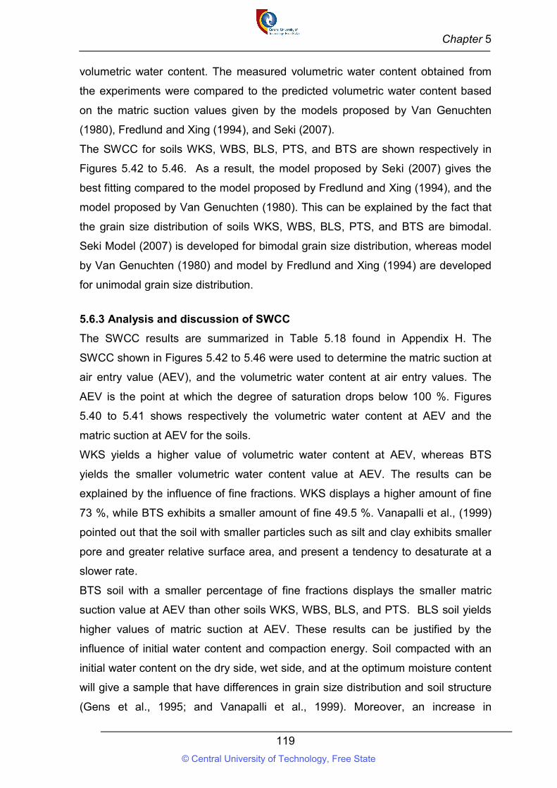
Chapter 5

119

volumetric water content. The measured volumetric water content obtained from

the experiments were compared to the predicted volumetric water content based

on the matric suction values given by the models proposed by Van Genuchten

(1980), Fredlund and Xing (1994), and Seki (2007).

The SWCC for soils WKS, WBS, BLS, PTS, and BTS are shown respectively in

Figures 5.42 to 5.46. As a result, the model proposed by Seki (2007) gives the

best fitting compared to the model proposed by Fredlund and Xing (1994), and the

model proposed by Van Genuchten (1980). This can be explained by the fact that

the grain size distribution of soils WKS, WBS, BLS, PTS, and BTS are bimodal.

Seki Model (2007) is developed for bimodal grain size distribution, whereas model

by Van Genuchten (1980) and model by Fredlund and Xing (1994) are developed

for unimodal grain size distribution.

5.6.3 Analysis and discussion of SWCC

The SWCC results are summarized in Table 5.18 found in Appendix H. The

SWCC shown in Figures 5.42 to 5.46 were used to determine the matric suction at

air entry value (AEV), and the volumetric water content at air entry values. The

AEV is the point at which the degree of saturation drops below 100 %. Figures

5.40 to 5.41 shows respectively the volumetric water content at AEV and the

matric suction at AEV for the soils.

WKS yields a higher value of volumetric water content at AEV, whereas BTS

yields the smaller volumetric water content value at AEV. The results can be

explained by the influence of fine fractions. WKS displays a higher amount of fine

73 %, while BTS exhibits a smaller amount of fine 49.5 %. Vanapalli et al., (1999)

pointed out that the soil with smaller particles such as silt and clay exhibits smaller

pore and greater relative surface area, and present a tendency to desaturate at a

slower rate.

BTS soil with a smaller percentage of fine fractions displays the smaller matric

suction value at AEV than other soils WKS, WBS, BLS, and PTS. BLS soil yields

higher values of matric suction at AEV. These results can be justified by the

influence of initial water content and compaction energy. Soil compacted with an

initial water content on the dry side, wet side, and at the optimum moisture content

will give a sample that have differences in grain size distribution and soil structure

(Gens et al., 1995; and Vanapalli et al., 1999). Moreover, an increase in


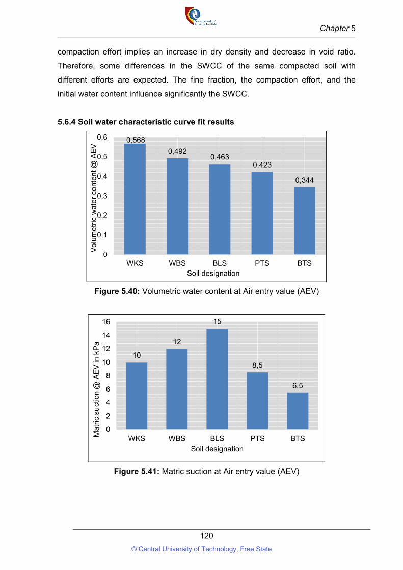
Chapter 5

120

compaction effort implies an increase in dry density and decrease in void ratio.

Therefore, some differences in the SWCC of the same compacted soil with

different efforts are expected. The fine fraction, the compaction effort, and the

initial water content influence significantly the SWCC.

5.6.4 Soil water characteristic curve fit results

Figure 5.40: Volumetric water content at Air entry value (AEV)

Figure 5.41: Matric suction at Air entry value (AEV)

0,568

0,4920,463

0,423

0,344

0

0,1

0,2

0,3

0,4

0,5

0,6

WKS WBS BLS PTS BTS

Vo

lum

etri

c w

ate

r co

nten

t @ A

EV

Soil designation

10

12

15

8,5

6,5

0

2

4

6

8

10

12

14

16

WKS WBS BLS PTS BTSMat

ric

suct

ion

@ A

EV

in k

Pa

Soil designation


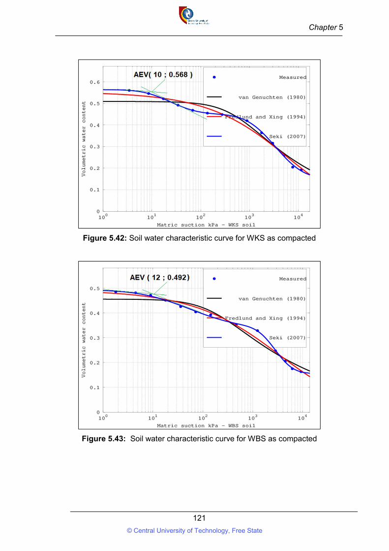
Chapter 5

121

Figure 5.42: Soil water characteristic curve for WKS as compacted

Figure 5.43: Soil water characteristic curve for WBS as compacted


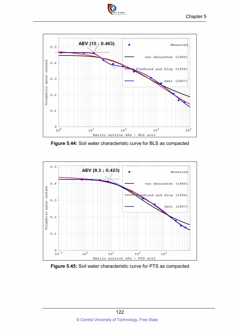
Chapter 5

122

Figure 5.44: Soil water characteristic curve for BLS as compacted

Figure 5.45: Soil water characteristic curve for PTS as compacted


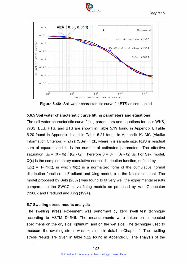
Chapter 5

123

Figure 5.46: Soil water characteristic curve for BTS as compacted

5.6.5 Soil water characteristic curve fitting parameters and equations

The soil water characteristic curve fitting parameters and equations for soils WKS,

WBS, BLS, PTS, and BTS are shown in Table 5.19 found in Appendix I, Table

5.20 found in Appendix J, and in Table 5.21 found in Appendix K. AIC (Akaike

Information Criterion) = n.ln (RSS/n) + 2k, where n is sample size, RSS is residual

sum of squares and ko is the number of estimated parameters. The effective

saturation, Se = (θ - θr) / (θs - θr). Therefore θ = θr + (θs - θr) Se. For Seki model,

Q(x) is the complementary cumulative normal distribution function, defined by

Q(x) = 1- Φ(x), in which Φ(x) is a normalized form of the cumulative normal

distribution function. In Fredlund and Xing model, e is the Napier constant. The

model proposed by Seki (2007) was found to fit very well the experimental results

compared to the SWCC curve fitting models as proposed by Van Genuchten

(1980); and Fredlund and Xing (1994).

5.7 Swelling stress results analysis

The swelling stress experiment was performed by zero swell test technique

according to ASTM D4546. The measurements were taken on compacted

specimens on the dry side, optimum, and on the wet side. The technique used to

measure the swelling stress was explained in detail in Chapter 4. The swelling

stress results are given in table 5.22 found in Appendix L. The analysis of the


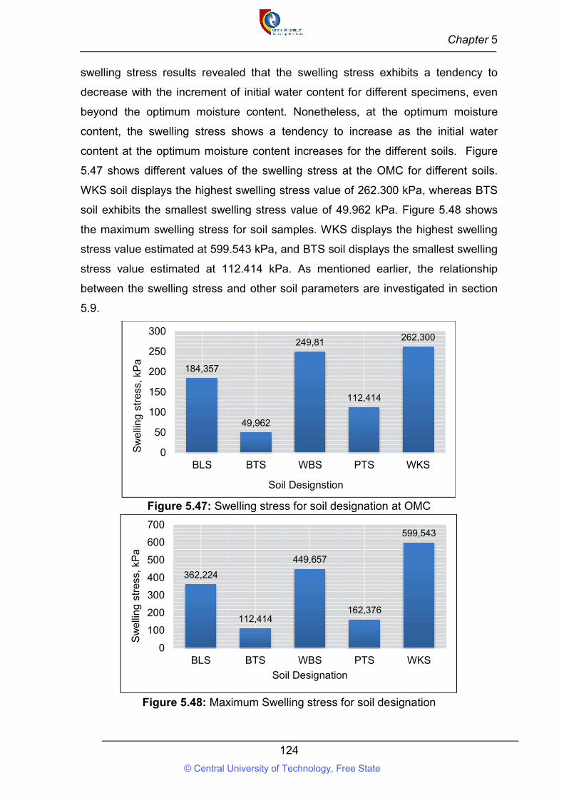
Chapter 5

124

swelling stress results revealed that the swelling stress exhibits a tendency to

decrease with the increment of initial water content for different specimens, even

beyond the optimum moisture content. Nonetheless, at the optimum moisture

content, the swelling stress shows a tendency to increase as the initial water

content at the optimum moisture content increases for the different soils. Figure

5.47 shows different values of the swelling stress at the OMC for different soils.

WKS soil displays the highest swelling stress value of 262.300 kPa, whereas BTS

soil exhibits the smallest swelling stress value of 49.962 kPa. Figure 5.48 shows

the maximum swelling stress for soil samples. WKS displays the highest swelling

stress value estimated at 599.543 kPa, and BTS soil displays the smallest swelling

stress value estimated at 112.414 kPa. As mentioned earlier, the relationship

between the swelling stress and other soil parameters are investigated in section

5.9.

Figure 5.47: Swelling stress for soil designation at OMC

Figure 5.48: Maximum Swelling stress for soil designation

184,357

49,962

249,81

112,414

262,300

0

50

100

150

200

250

300

BLS BTS WBS PTS WKS

Sw

ellin

g s

tres

s, k

Pa

Soil Designstion

362,224

112,414

449,657

162,376

599,543

0

100

200

300

400

500

600

700

BLS BTS WBS PTS WKS

Sw

ellin

g s

tres

s, k

Pa

Soil Designation


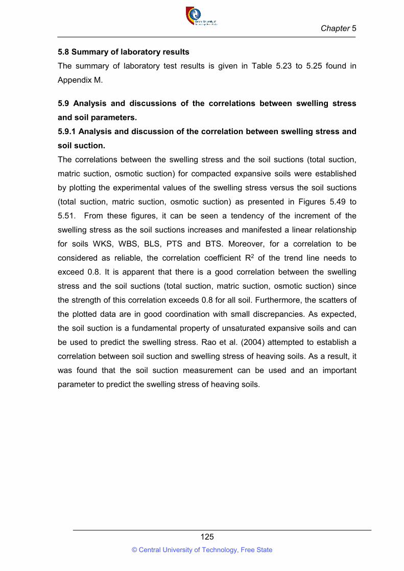
Chapter 5

125

5.8 Summary of laboratory results

The summary of laboratory test results is given in Table 5.23 to 5.25 found in

Appendix M.

5.9 Analysis and discussions of the correlations between swelling stress

and soil parameters.

5.9.1 Analysis and discussion of the correlation between swelling stress and

soil suction.

The correlations between the swelling stress and the soil suctions (total suction,

matric suction, osmotic suction) for compacted expansive soils were established

by plotting the experimental values of the swelling stress versus the soil suctions

(total suction, matric suction, osmotic suction) as presented in Figures 5.49 to

5.51. From these figures, it can be seen a tendency of the increment of the

swelling stress as the soil suctions increases and manifested a linear relationship

for soils WKS, WBS, BLS, PTS and BTS. Moreover, for a correlation to be

considered as reliable, the correlation coefficient R2 of the trend line needs to

exceed 0.8. It is apparent that there is a good correlation between the swelling

stress and the soil suctions (total suction, matric suction, osmotic suction) since

the strength of this correlation exceeds 0.8 for all soil. Furthermore, the scatters of

the plotted data are in good coordination with small discrepancies. As expected,

the soil suction is a fundamental property of unsaturated expansive soils and can

be used to predict the swelling stress. Rao et al. (2004) attempted to establish a

correlation between soil suction and swelling stress of heaving soils. As a result, it

was found that the soil suction measurement can be used and an important

parameter to predict the swelling stress of heaving soils.


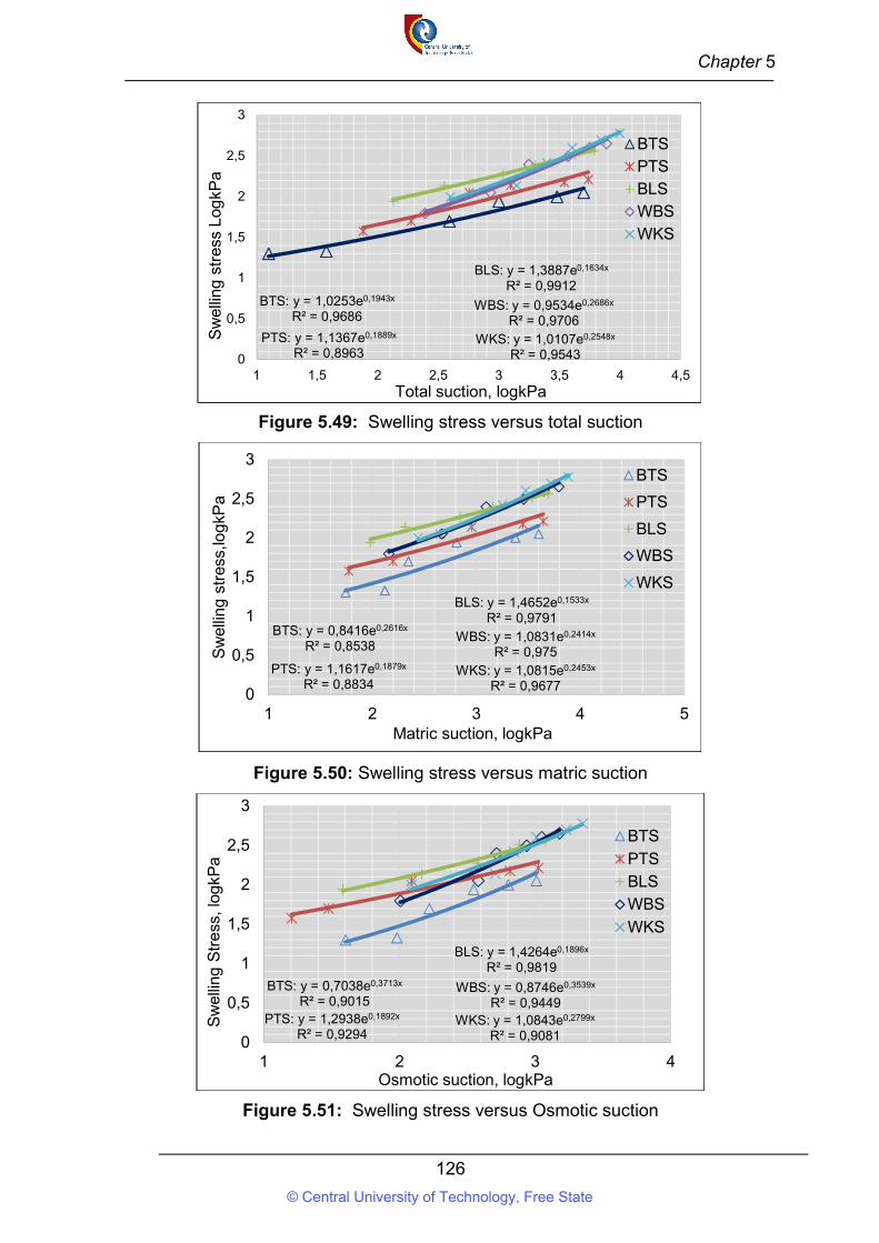
Chapter 5

126

Figure 5.49: Swelling stress versus total suction

Figure 5.50: Swelling stress versus matric suction

Figure 5.51: Swelling stress versus Osmotic suction

BTS: y = 1,0253e0,1943x

R² = 0,9686

PTS: y = 1,1367e0,1889x

R² = 0,8963

BLS: y = 1,3887e0,1634x

R² = 0,9912

WBS: y = 0,9534e0,2686x

R² = 0,9706WKS: y = 1,0107e0,2548x

R² = 0,95430

0,5

1

1,5

2

2,5

3

1 1,5 2 2,5 3 3,5 4 4,5

Sw

ellin

g s

tres

s L

ogkP

a

Total suction, logkPa

BTSPTSBLSWBSWKS

BTS: y = 0,8416e0,2616x

R² = 0,8538

PTS: y = 1,1617e0,1879x

R² = 0,8834

BLS: y = 1,4652e0,1533x

R² = 0,9791

WBS: y = 1,0831e0,2414x

R² = 0,975WKS: y = 1,0815e0,2453x

R² = 0,96770

0,5

1

1,5

2

2,5

3

1 2 3 4 5

Sw

ellin

g s

tres

s,lo

gkP

a

Matric suction, logkPa

BTS

PTS

BLS

WBS

WKS

BTS: y = 0,7038e0,3713x

R² = 0,9015PTS: y = 1,2938e0,1892x

R² = 0,9294

BLS: y = 1,4264e0,1896x

R² = 0,9819

WBS: y = 0,8746e0,3539x

R² = 0,9449WKS: y = 1,0843e0,2799x

R² = 0,90810

0,5

1

1,5

2

2,5

3

1 2 3 4

Sw

ellin

g S

tre

ss, l

ogkP

a

Osmotic suction, logkPa

BTS

PTSBLSWBS

WKS


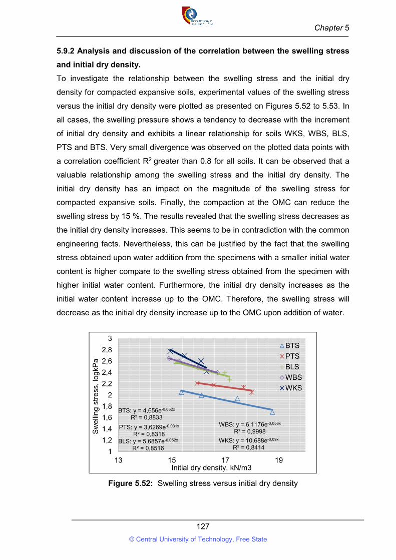
Chapter 5

127

5.9.2 Analysis and discussion of the correlation between the swelling stress

and initial dry density.

To investigate the relationship between the swelling stress and the initial dry

density for compacted expansive soils, experimental values of the swelling stress

versus the initial dry density were plotted as presented on Figures 5.52 to 5.53. In

all cases, the swelling pressure shows a tendency to decrease with the increment

of initial dry density and exhibits a linear relationship for soils WKS, WBS, BLS,

PTS and BTS. Very small divergence was observed on the plotted data points with

a correlation coefficient R2 greater than 0.8 for all soils. It can be observed that a

valuable relationship among the swelling stress and the initial dry density. The

initial dry density has an impact on the magnitude of the swelling stress for

compacted expansive soils. Finally, the compaction at the OMC can reduce the

swelling stress by 15 %. The results revealed that the swelling stress decreases as

the initial dry density increases. This seems to be in contradiction with the common

engineering facts. Nevertheless, this can be justified by the fact that the swelling

stress obtained upon water addition from the specimens with a smaller initial water

content is higher compare to the swelling stress obtained from the specimen with

higher initial water content. Furthermore, the initial dry density increases as the

initial water content increase up to the OMC. Therefore, the swelling stress will

decrease as the initial dry density increase up to the OMC upon addition of water.

Figure 5.52: Swelling stress versus initial dry density

BTS: y = 4,656e-0,052x

R² = 0,8833

PTS: y = 3,6269e-0,031x

R² = 0,8318BLS: y = 5,6857e-0,052x

R² = 0,8516

WBS: y = 6,1176e-0,056x

R² = 0,9998

WKS: y = 10,688e-0,09x

R² = 0,84141

1,2

1,4

1,6

1,8

2

2,2

2,4

2,6

2,8

3

13 15 17 19

Sw

ellin

g s

tres

s, lo

gkP

a

Initial dry density, kN/m3

BTS

PTS

BLS

WBS

WKS


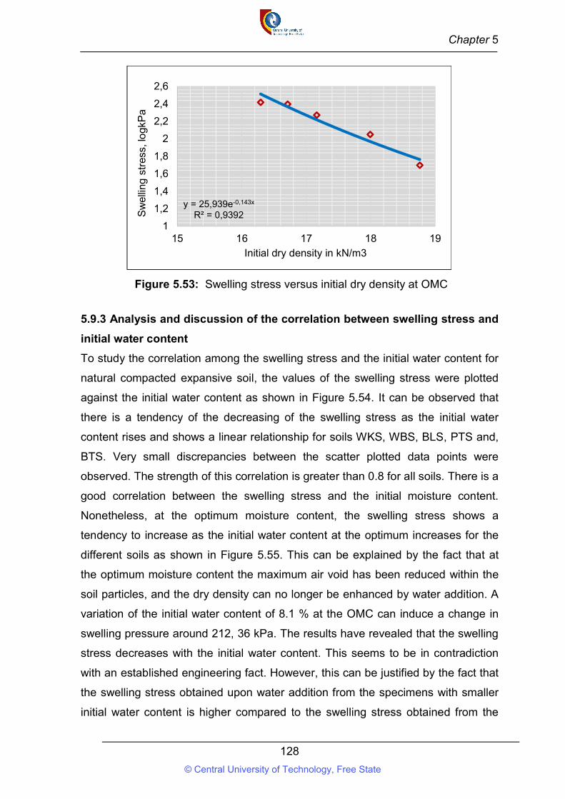
Chapter 5

128

Figure 5.53: Swelling stress versus initial dry density at OMC


initial water content

To study the correlation among the swelling stress and the initial water content for

natural compacted expansive soil, the values of the swelling stress were plotted

against the initial water content as shown in Figure 5.54. It can be observed that

there is a tendency of the decreasing of the swelling stress as the initial water

content rises and shows a linear relationship for soils WKS, WBS, BLS, PTS and,

BTS. Very small discrepancies between the scatter plotted data points were

observed. The strength of this correlation is greater than 0.8 for all soils. There is a

good correlation between the swelling stress and the initial moisture content.

Nonetheless, at the optimum moisture content, the swelling stress shows a

tendency to increase as the initial water content at the optimum increases for the

different soils as shown in Figure 5.55. This can be explained by the fact that at

the optimum moisture content the maximum air void has been reduced within the

soil particles, and the dry density can no longer be enhanced by water addition. A

variation of the initial water content of 8.1 % at the OMC can induce a change in

swelling pressure around 212, 36 kPa. The results have revealed that the swelling

stress decreases with the initial water content. This seems to be in contradiction

with an established engineering fact. However, this can be justified by the fact that

the swelling stress obtained upon water addition from the specimens with smaller

initial water content is higher compared to the swelling stress obtained from the

y = 25,939e-0,143x

R² = 0,93921

1,2

1,4

1,6

1,8

2

2,2

2,4

2,6

15 16 17 18 19

Sw

ellin

g s

tres

s, lo

gkP

a

Initial dry density in kN/m3


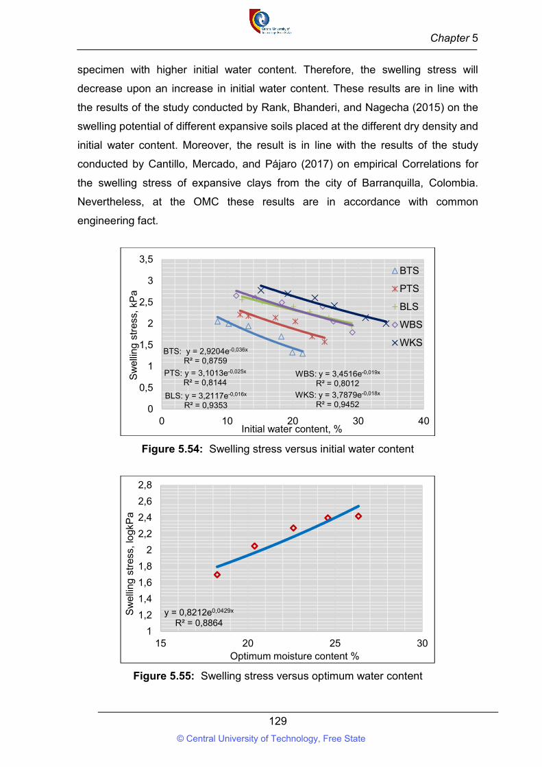
Chapter 5

129

specimen with higher initial water content. Therefore, the swelling stress will

decrease upon an increase in initial water content. These results are in line with

the results of the study conducted by Rank, Bhanderi, and Nagecha (2015) on the

swelling potential of different expansive soils placed at the different dry density and

initial water content. Moreover, the result is in line with the results of the study

conducted by Cantillo, Mercado, and Pájaro (2017) on empirical Correlations for

the swelling stress of expansive clays from the city of Barranquilla, Colombia.

Nevertheless, at the OMC these results are in accordance with common

engineering fact.

Figure 5.54: Swelling stress versus initial water content

Figure 5.55: Swelling stress versus optimum water content

BTS: y = 2,9204e-0,036x

R² = 0,8759

PTS: y = 3,1013e-0,025x

R² = 0,8144

BLS: y = 3,2117e-0,016x

R² = 0,9353

WBS: y = 3,4516e-0,019x

R² = 0,8012

WKS: y = 3,7879e-0,018x

R² = 0,94520

0,5

1

1,5

2

2,5

3

3,5

0 10 20 30 40

Sw

ellin

g s

tres

s, k

Pa

Initial water content, %

BTS

PTS

BLS

WBS

WKS

y = 0,8212e0,0429x

R² = 0,88641

1,2

1,4

1,6

1,8

2

2,2

2,4

2,6

2,8

15 20 25 30

Sw

ellin

g s

tres

s, lo

gkP

a

Optimum moisture content %


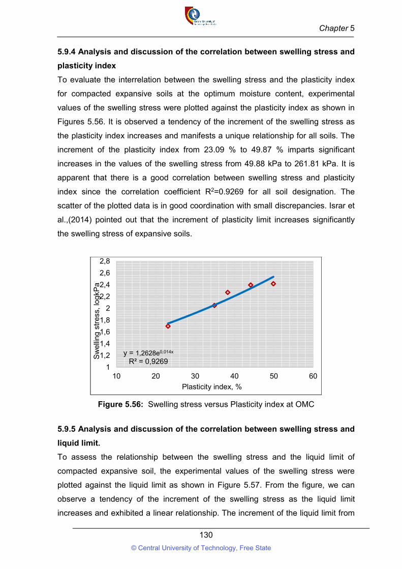
Chapter 5

130


plasticity index

To evaluate the interrelation between the swelling stress and the plasticity index

for compacted expansive soils at the optimum moisture content, experimental

values of the swelling stress were plotted against the plasticity index as shown in

Figures 5.56. It is observed a tendency of the increment of the swelling stress as

the plasticity index increases and manifests a unique relationship for all soils. The

increment of the plasticity index from 23.09 % to 49.87 % imparts significant

increases in the values of the swelling stress from 49.88 kPa to 261.81 kPa. It is

apparent that there is a good correlation between swelling stress and plasticity

index since the correlation coefficient R2=0.9269 for all soil designation. The

scatter of the plotted data is in good coordination with small discrepancies. Israr et

al.,(2014) pointed out that the increment of plasticity limit increases significantly

the swelling stress of expansive soils.

Figure 5.56: Swelling stress versus Plasticity index at OMC


liquid limit.

To assess the relationship between the swelling stress and the liquid limit of

compacted expansive soil, the experimental values of the swelling stress were

plotted against the liquid limit as shown in Figure 5.57. From the figure, we can

observe a tendency of the increment of the swelling stress as the liquid limit

increases and exhibited a linear relationship. The increment of the liquid limit from

y = 1,2628e0,014x

R² = 0,92691

1,2

1,4

1,6

1,8

2

2,2

2,4

2,6

2,8

10 20 30 40 50 60

Sw

ellin

g s

tres

s, lo

gkP

a

Plasticity index, %


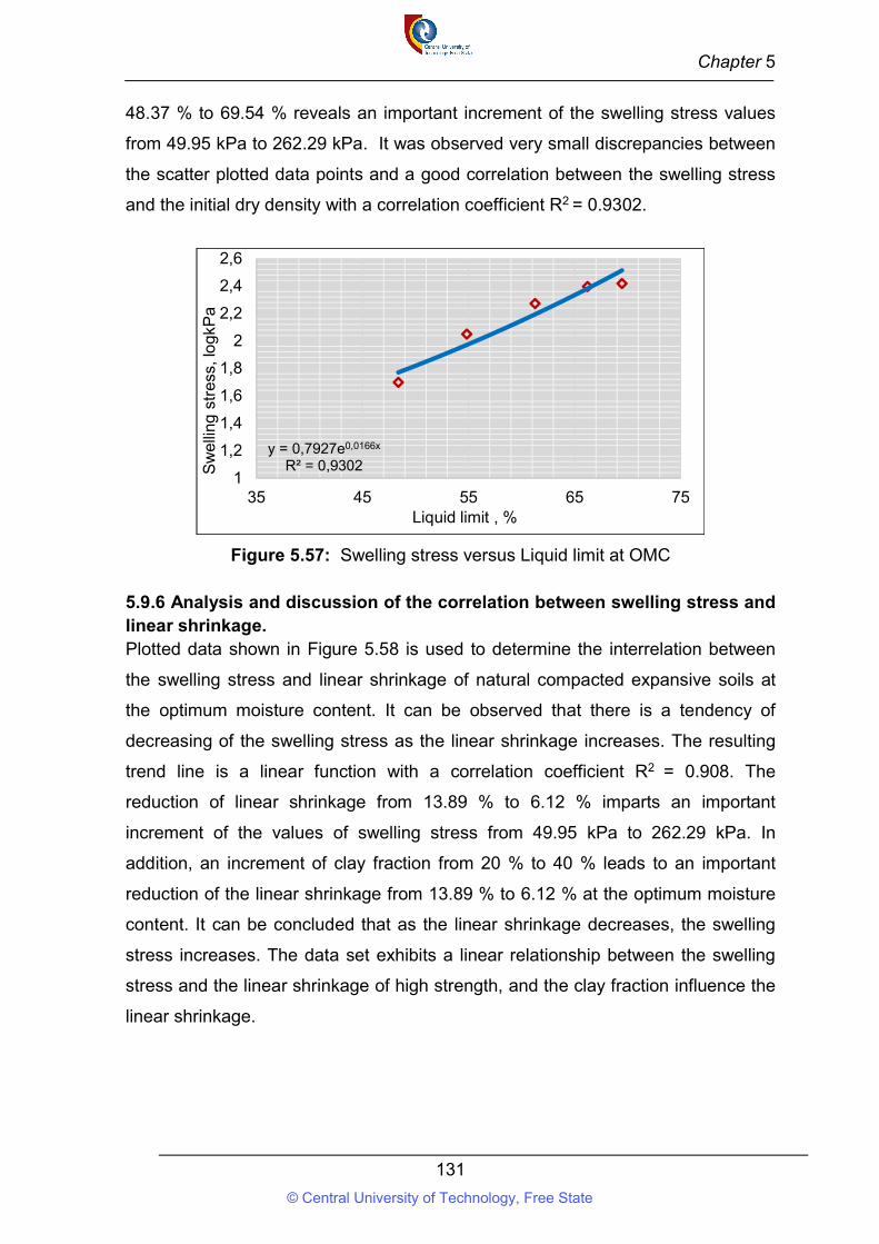
Chapter 5

131

48.37 % to 69.54 % reveals an important increment of the swelling stress values

from 49.95 kPa to 262.29 kPa. It was observed very small discrepancies between

the scatter plotted data points and a good correlation between the swelling stress

and the initial dry density with a correlation coefficient R2 = 0.9302.

Figure 5.57: Swelling stress versus Liquid limit at OMC

5.9.6 Analysis and discussion of the correlation between swelling stress and linear shrinkage. Plotted data shown in Figure 5.58 is used to determine the interrelation between

the swelling stress and linear shrinkage of natural compacted expansive soils at

the optimum moisture content. It can be observed that there is a tendency of

decreasing of the swelling stress as the linear shrinkage increases. The resulting

trend line is a linear function with a correlation coefficient R2 = 0.908. The

reduction of linear shrinkage from 13.89 % to 6.12 % imparts an important

increment of the values of swelling stress from 49.95 kPa to 262.29 kPa. In

addition, an increment of clay fraction from 20 % to 40 % leads to an important

reduction of the linear shrinkage from 13.89 % to 6.12 % at the optimum moisture

content. It can be concluded that as the linear shrinkage decreases, the swelling

stress increases. The data set exhibits a linear relationship between the swelling

stress and the linear shrinkage of high strength, and the clay fraction influence the

linear shrinkage.

y = 0,7927e0,0166x

R² = 0,93021

1,2

1,4

1,6

1,8

2

2,2

2,4

2,6

35 45 55 65 75

Sw

ellin

g s

tres

s, lo

gkP

a

Liquid limit , %


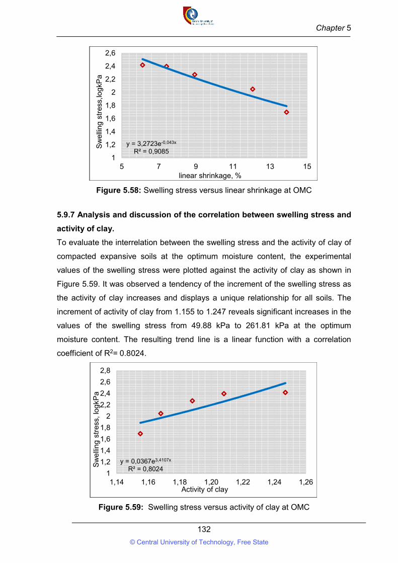
Chapter 5

132

Figure 5.58: Swelling stress versus linear shrinkage at OMC


activity of clay.

To evaluate the interrelation between the swelling stress and the activity of clay of

compacted expansive soils at the optimum moisture content, the experimental

values of the swelling stress were plotted against the activity of clay as shown in

Figure 5.59. It was observed a tendency of the increment of the swelling stress as

the activity of clay increases and displays a unique relationship for all soils. The

increment of activity of clay from 1.155 to 1.247 reveals significant increases in the

values of the swelling stress from 49.88 kPa to 261.81 kPa at the optimum

moisture content. The resulting trend line is a linear function with a correlation

coefficient of R2= 0.8024.

Figure 5.59: Swelling stress versus activity of clay at OMC

y = 3,2723e-0,043x

R² = 0,90851

1,2

1,4

1,6

1,8

2

2,2

2,4

2,6

5 7 9 11 13 15

Sw

ellin

g s

tres

s,lo

gkP

a

linear shrinkage, %

y = 0,0367e3,4107x

R² = 0,80241

1,2

1,4

1,6

1,8

2

2,2

2,4

2,6

2,8

1,14 1,16 1,18 1,20 1,22 1,24 1,26

Sw

ellin

g s

tres

s, lo

gkP

a

Activity of clay


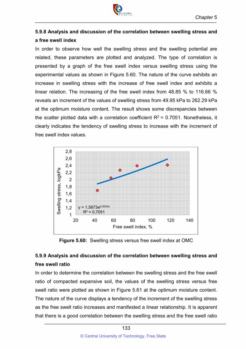
Chapter 5

133


a free swell index

In order to observe how well the swelling stress and the swelling potential are

related, these parameters are plotted and analyzed. The type of correlation is

presented by a graph of the free swell index versus swelling stress using the

experimental values as shown in Figure 5.60. The nature of the curve exhibits an

increase in swelling stress with the increase of free swell index and exhibits a

linear relation. The increasing of the free swell index from 48.85 % to 116.66 %

reveals an increment of the values of swelling stress from 49.95 kPa to 262.29 kPa

at the optimum moisture content. The result shows some discrepancies between

the scatter plotted data with a correlation coefficient R2 = 0.7051. Nonetheless, it

clearly indicates the tendency of swelling stress to increase with the increment of

free swell index values.

Figure 5.60: Swelling stress versus free swell index at OMC


free swell ratio

In order to determine the correlation between the swelling stress and the free swell

ratio of compacted expansive soil, the values of the swelling stress versus free

swell ratio were plotted as shown in Figure 5.61 at the optimum moisture content.

The nature of the curve displays a tendency of the increment of the swelling stress

as the free swell ratio increases and manifested a linear relationship. It is apparent

that there is a good correlation between the swelling stress and the free swell ratio

y = 1,5673e0,0043x

R² = 0,70511

1,2

1,4

1,6

1,8

2

2,2

2,4

2,6

2,8

20 40 60 80 100 120 140

Sw

ellin

g s

tres

s, lo

gkP

a

Free swell index, %


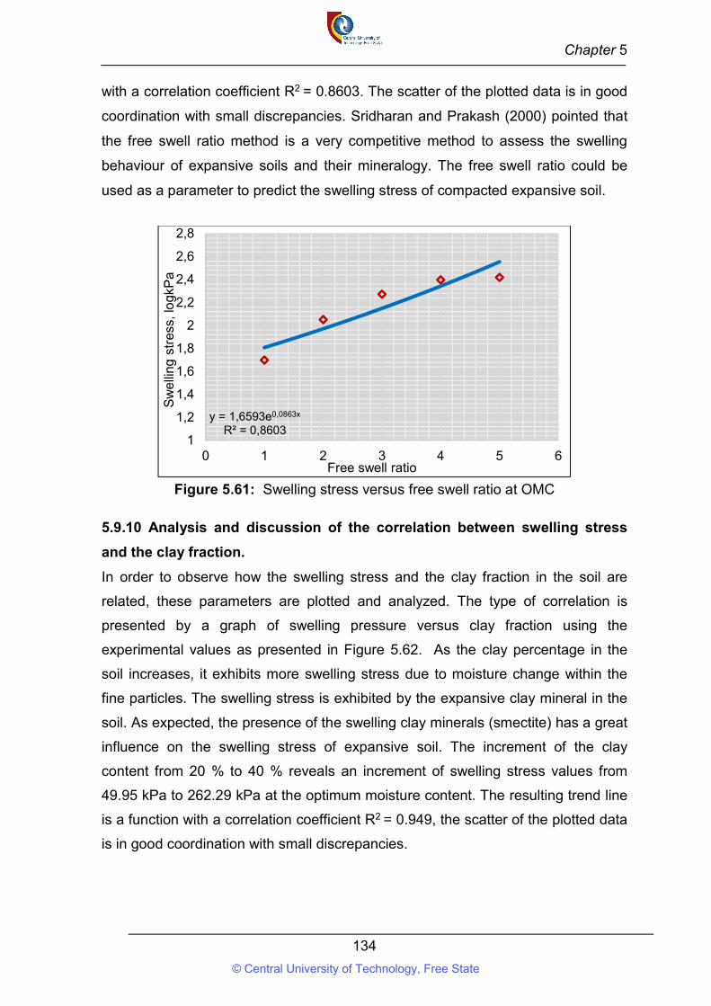
Chapter 5

134

with a correlation coefficient R2 = 0.8603. The scatter of the plotted data is in good

coordination with small discrepancies. Sridharan and Prakash (2000) pointed that

the free swell ratio method is a very competitive method to assess the swelling

behaviour of expansive soils and their mineralogy. The free swell ratio could be

used as a parameter to predict the swelling stress of compacted expansive soil.

Figure 5.61: Swelling stress versus free swell ratio at OMC

5.9.10 Analysis and discussion of the correlation between swelling stress

and the clay fraction.

In order to observe how the swelling stress and the clay fraction in the soil are

related, these parameters are plotted and analyzed. The type of correlation is

presented by a graph of swelling pressure versus clay fraction using the

experimental values as presented in Figure 5.62. As the clay percentage in the

soil increases, it exhibits more swelling stress due to moisture change within the

fine particles. The swelling stress is exhibited by the expansive clay mineral in the

soil. As expected, the presence of the swelling clay minerals (smectite) has a great

influence on the swelling stress of expansive soil. The increment of the clay

content from 20 % to 40 % reveals an increment of swelling stress values from

49.95 kPa to 262.29 kPa at the optimum moisture content. The resulting trend line

is a function with a correlation coefficient R2 = 0.949, the scatter of the plotted data

is in good coordination with small discrepancies.

y = 1,6593e0,0863x

R² = 0,86031

1,2

1,4

1,6

1,8

2

2,2

2,4

2,6

2,8

0 1 2 3 4 5 6

Sw

ellin

g s

tres

s, lo

gkP

a

Free swell ratio


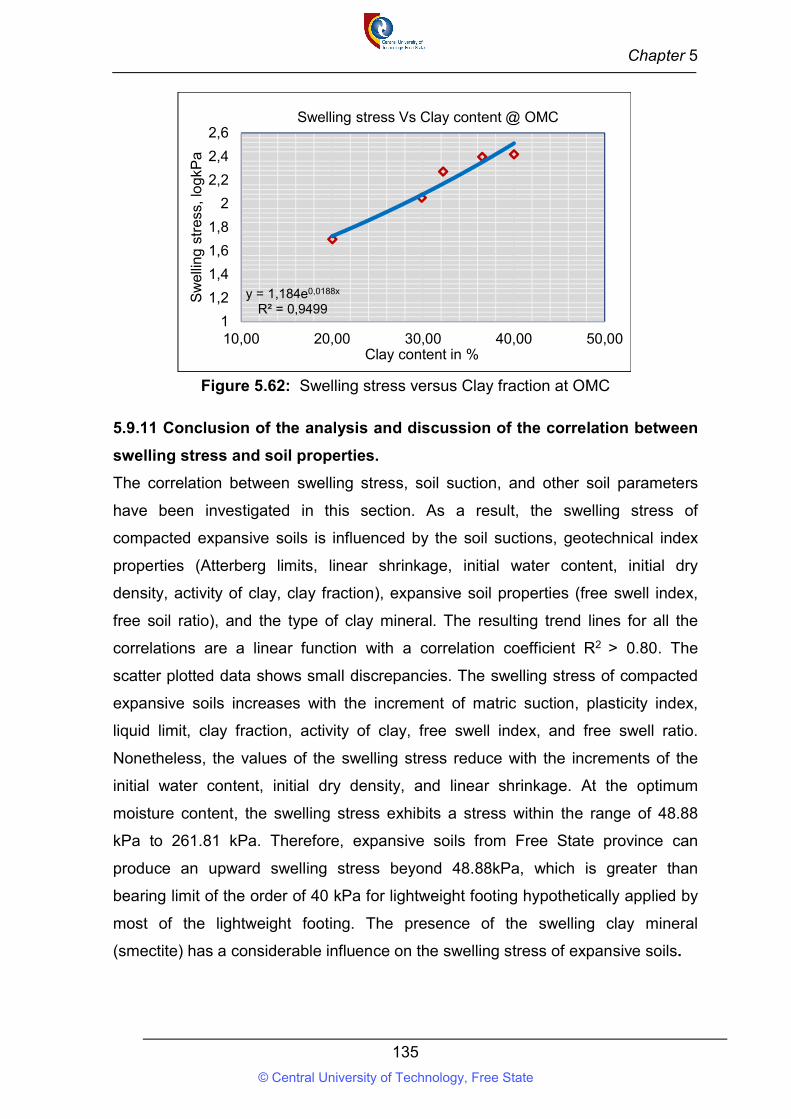
Chapter 5

135

Figure 5.62: Swelling stress versus Clay fraction at OMC

5.9.11 Conclusion of the analysis and discussion of the correlation between

swelling stress and soil properties.

The correlation between swelling stress, soil suction, and other soil parameters

have been investigated in this section. As a result, the swelling stress of

compacted expansive soils is influenced by the soil suctions, geotechnical index

properties (Atterberg limits, linear shrinkage, initial water content, initial dry

density, activity of clay, clay fraction), expansive soil properties (free swell index,

free soil ratio), and the type of clay mineral. The resulting trend lines for all the

correlations are a linear function with a correlation coefficient R2 > 0.80. The

scatter plotted data shows small discrepancies. The swelling stress of compacted

expansive soils increases with the increment of matric suction, plasticity index,

liquid limit, clay fraction, activity of clay, free swell index, and free swell ratio.

Nonetheless, the values of the swelling stress reduce with the increments of the

initial water content, initial dry density, and linear shrinkage. At the optimum

moisture content, the swelling stress exhibits a stress within the range of 48.88

kPa to 261.81 kPa. Therefore, expansive soils from Free State province can

produce an upward swelling stress beyond 48.88kPa, which is greater than

bearing limit of the order of 40 kPa for lightweight footing hypothetically applied by

most of the lightweight footing. The presence of the swelling clay mineral

(smectite) has a considerable influence on the swelling stress of expansive soils.

y = 1,184e0,0188x

R² = 0,94991

1,2

1,4

1,6

1,8

2

2,2

2,4

2,6

10,00 20,00 30,00 40,00 50,00

Sw

ellin

g s

tres

s, lo

gkP

a

Clay content in %

Swelling stress Vs Clay content @ OMC


Chapter 5

136

5.10 Constitutive models to predict the swelling stress.

The characterization of the relation between swelling stress and soil properties

was performed by investigating the nature of the correlation between the swelling

stress, the suction matric, and other soil properties. Moreover, the characterization

of the swelling stress and the soil properties relationship for compacted

unsaturated expansive soils is achieved by developing models to predict the

swelling stress with respect to the suction matric, and other soil properties such as

initial water content, initial dry density, plasticity index, liquid limit, linear shrinkage,

activity of clay, free swell index, and free swell ratio. A series of efficient

combinations of suction matric and other soils properties are used as independent

variables to develop the models as explained in chapter 4, section 4.8.

5.10.1 Determination of the models, multi-regression analysis coefficients,

intercepts, and regression statistics.

The correlation Matrix A, and correlation Matrix B are shown respectively in Tables

5.26 found in Appendix N, and in Table 5.27 Found in Appendix O are used for

multi-regression analysis.

Six models to predict the swelling stress of field compacted expansive soils were

developed:

Model (1) is established with the following independent variables: matric suction

(ψ ), liquid limit (LL), initial dry density (γ ), activity of clay (A ), with coefficients of

correlation λ , λ ,λ , λ , and the intercept λ .

Model (2) is built up with the following independent variables: matric suction (ψ ),

initial water content (W ), liquid limit (LL), activity of clay (A ), with coefficients of

correlation η , η ,η , η , and the intercept η .

Model (3) is developed with the following independent variables: matric suction

(ψ ), initial water content (W ), Plasticity (PI), liquid limit (LL), activity of clay (A ),

with coefficients of correlation ξ , ξ ,ξ , ξ , ξ and the intercept ξ .

Model (4) is formed with the following independent variables: matric suction (ψ ),

plasticity index(PI), initial water content (W ), linear shrinkage (LS), free swell ratio

(FSR), with coefficients of correlation ζ , ζ , ζ , ζ , ζ and the intercept ζ .


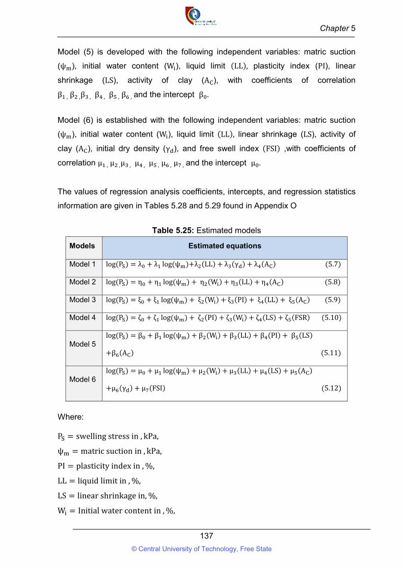
Chapter 5

137

Model (5) is developed with the following independent variables: matric suction

(ψ ), initial water content (W ), liquid limit (LL), plasticity index (PI), linear

shrinkage (LS), activity of clay (A ), with coefficients of correlation

β , β ,β , β , β , β , and the intercept β .

Model (6) is established with the following independent variables: matric suction

(ψ ), initial water content (W ), liquid limit (LL), linear shrinkage (LS), activity of

clay (A ), initial dry density (γ ), and free swell index (FSI) ,with coefficients of

correlation μ , μ ,μ , μ , μ , μ , μ , and the intercept μ .

The values of regression analysis coefficients, intercepts, and regression statistics

information are given in Tables 5.28 and 5.29 found in Appendix O

Table 5.25: Estimated models

Models Estimated equations

Model 1 log (P ) = λ + λ log(ψ )+λ (LL) + λ (γ ) + λ (A ) (5.7)

Model 2 log (P ) = η + η log(ψ ) + η (W ) + η (LL) + η (A ) (5.8)

Model 3 log (P ) = ξ + ξ log(ψ ) + ξ (W ) + ξ (PI) + ξ (LL) + ξ (A ) (5.9)

Model 4 log (P ) = ζ + ζ log(ψ ) + ζ (PI) + ζ (W ) + ζ (LS) + ζ (FSR) (5.10)

Model 5 log (P ) = β + β log(ψ ) + β (W ) + β (LL) + β (PI) + β (LS)

+β (A ) (5.11)

Model 6 log (P ) = μ + μ log(ψ ) + μ (W ) + μ (LL) + μ (LS) + μ (A )

+μ (γ ) + μ (FSI) (5.12)

Where:

P = swelling stress in , kPa,

ψ = matric suction in , kPa,

PI = plasticity index in , %,

LL = liquid limit in , %,

LS = linear shrinkage in, %,

W = Initial water content in , %,


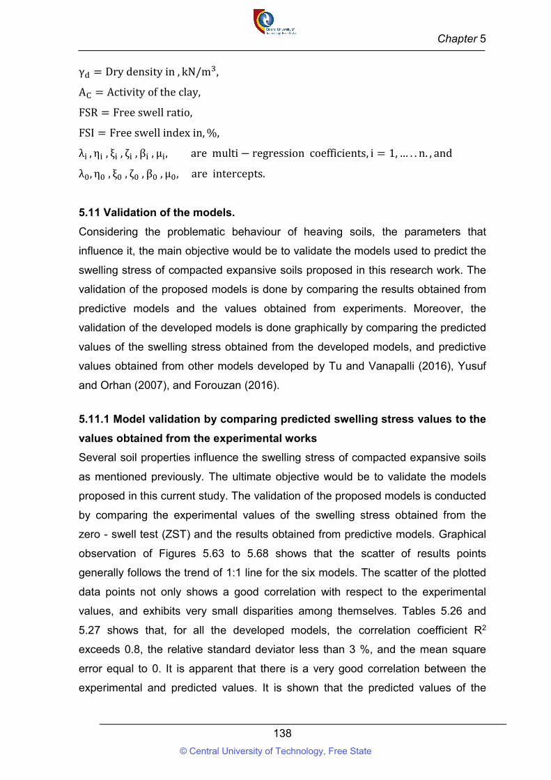
Chapter 5

138

γ = Dry density in , kN/m ,

A = Activity of the clay,

FSR = Free swell ratio,

FSI = Free swell index in, %,

λ , η , ξ , ζ , β , μ , are multi − regression coefficients, i = 1, … . . n. , and

λ , η , ξ , ζ , β , μ , are intercepts.

5.11 Validation of the models.

Considering the problematic behaviour of heaving soils, the parameters that

influence it, the main objective would be to validate the models used to predict the

swelling stress of compacted expansive soils proposed in this research work. The

validation of the proposed models is done by comparing the results obtained from

predictive models and the values obtained from experiments. Moreover, the

validation of the developed models is done graphically by comparing the predicted

values of the swelling stress obtained from the developed models, and predictive

values obtained from other models developed by Tu and Vanapalli (2016), Yusuf

and Orhan (2007), and Forouzan (2016).

5.11.1 Model validation by comparing predicted swelling stress values to the

values obtained from the experimental works

Several soil properties influence the swelling stress of compacted expansive soils

as mentioned previously. The ultimate objective would be to validate the models

proposed in this current study. The validation of the proposed models is conducted

by comparing the experimental values of the swelling stress obtained from the

zero - swell test (ZST) and the results obtained from predictive models. Graphical

observation of Figures 5.63 to 5.68 shows that the scatter of results points

generally follows the trend of 1:1 line for the six models. The scatter of the plotted

data points not only shows a good correlation with respect to the experimental

values, and exhibits very small disparities among themselves. Tables 5.26 and

5.27 shows that, for all the developed models, the correlation coefficient R2

exceeds 0.8, the relative standard deviator less than 3 %, and the mean square

error equal to 0. It is apparent that there is a very good correlation between the

experimental and predicted values. It is shown that the predicted values of the


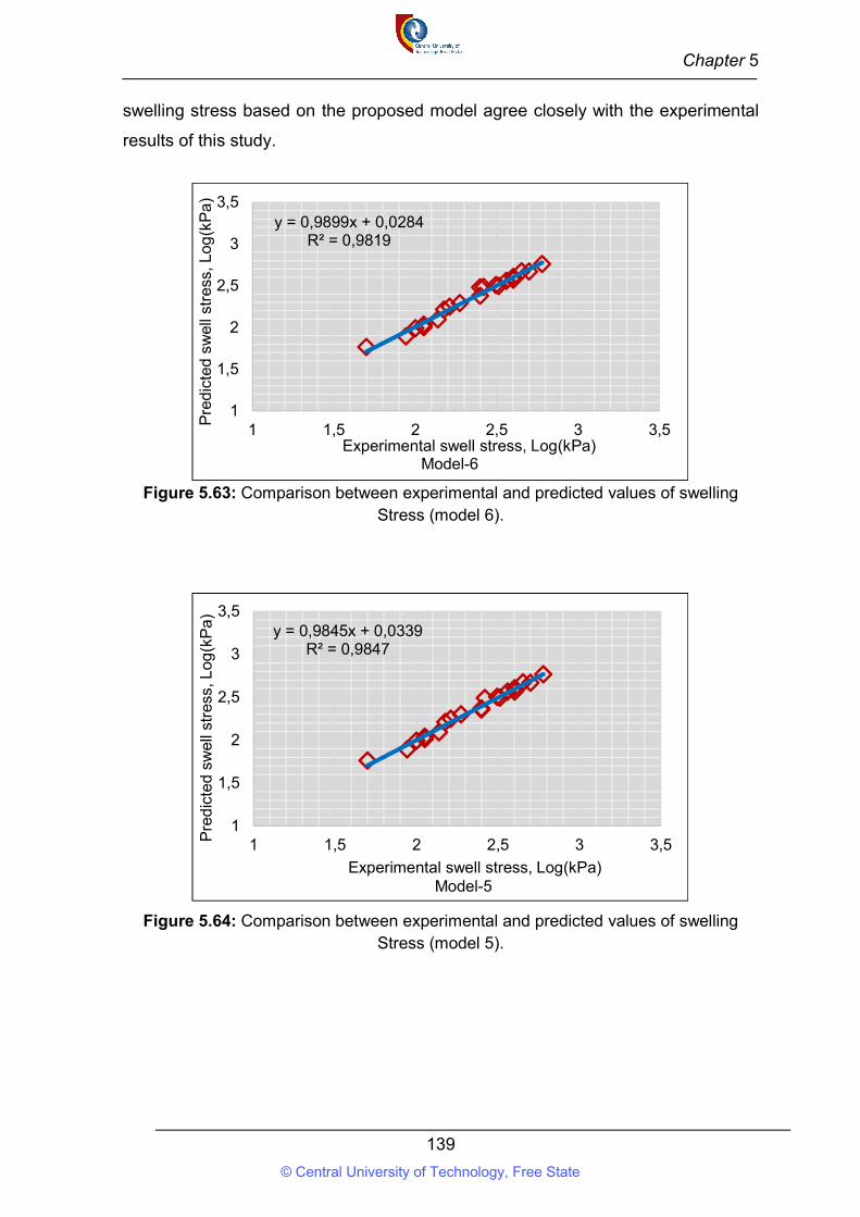
Chapter 5

139

swelling stress based on the proposed model agree closely with the experimental

results of this study.

Figure 5.63: Comparison between experimental and predicted values of swelling

Stress (model 6).

Figure 5.64: Comparison between experimental and predicted values of swelling Stress (model 5).

y = 0,9899x + 0,0284R² = 0,9819

1

1,5

2

2,5

3

3,5

1 1,5 2 2,5 3 3,5

Pre

dic

ted

sw

ell s

tres

s, L

og(k

Pa)

Experimental swell stress, Log(kPa)Model-6

y = 0,9845x + 0,0339R² = 0,9847

1

1,5

2

2,5

3

3,5

1 1,5 2 2,5 3 3,5Pre

dic

ted

sw

ell s

tres

s, L

og(k

Pa)



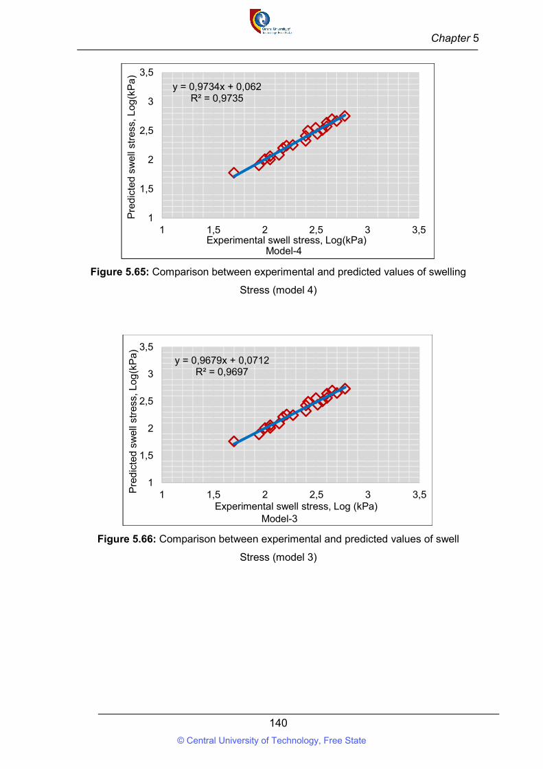
Chapter 5

140


Stress (model 4)

Figure 5.66: Comparison between experimental and predicted values of swell

Stress (model 3)

y = 0,9734x + 0,062R² = 0,9735

1

1,5

2

2,5

3

3,5

1 1,5 2 2,5 3 3,5

Pre

dic

ted

sw

ell s

tres

s, L

og(k

Pa)


y = 0,9679x + 0,0712R² = 0,9697

1

1,5

2

2,5

3

3,5

1 1,5 2 2,5 3 3,5Pre

dic

ted

sw

ell s

tres

s, L

og(k

Pa)

Experimental swell stress, Log (kPa)Model-3


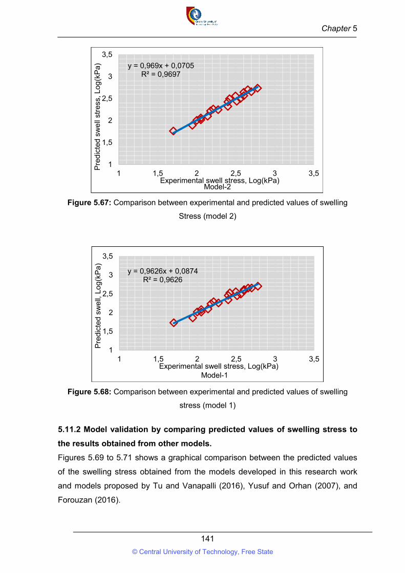
Chapter 5

141


Stress (model 2)


stress (model 1)

5.11.2 Model validation by comparing predicted values of swelling stress to

the results obtained from other models.

Figures 5.69 to 5.71 shows a graphical comparison between the predicted values

of the swelling stress obtained from the models developed in this research work

and models proposed by Tu and Vanapalli (2016), Yusuf and Orhan (2007), and

Forouzan (2016).

y = 0,969x + 0,0705R² = 0,9697

1

1,5

2

2,5

3

3,5

1 1,5 2 2,5 3 3,5

Pre

dic

ted

sw

ell s

tres

s, L

og(k

Pa)


y = 0,9626x + 0,0874R² = 0,9626

1

1,5

2

2,5

3

3,5

1 1,5 2 2,5 3 3,5

Pre

dic

ted

sw

ell,

Log

(kP

a)



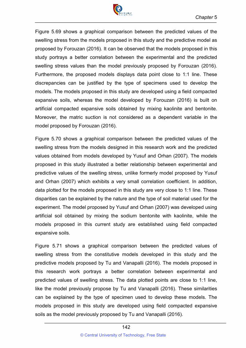
Chapter 5

142

Figure 5.69 shows a graphical comparison between the predicted values of the

swelling stress from the models proposed in this study and the predictive model as

proposed by Forouzan (2016). It can be observed that the models proposed in this

study portrays a better correlation between the experimental and the predicted

swelling stress values than the model previously proposed by Forouzan (2016).

Furthermore, the proposed models displays data point close to 1:1 line. These

discrepancies can be justified by the type of specimens used to develop the

models. The models proposed in this study are developed using a field compacted

expansive soils, whereas the model developed by Forouzan (2016) is built on

artificial compacted expansive soils obtained by mixing kaolinite and bentonite.

Moreover, the matric suction is not considered as a dependent variable in the

model proposed by Forouzan (2016).

Figure 5.70 shows a graphical comparison between the predicted values of the

swelling stress from the models designed in this research work and the predicted

values obtained from models developed by Yusuf and Orhan (2007). The models

proposed in this study illustrated a better relationship between experimental and

predictive values of the swelling stress, unlike formerly model proposed by Yusuf

and Orhan (2007) which exhibits a very small correlation coefficient. In addition,

data plotted for the models proposed in this study are very close to 1:1 line. These

disparities can be explained by the nature and the type of soil material used for the

experiment. The model proposed by Yusuf and Orhan (2007) was developed using

artificial soil obtained by mixing the sodium bentonite with kaolinite, while the

models proposed in this current study are established using field compacted

expansive soils.

Figure 5.71 shows a graphical comparison between the predicted values of

swelling stress from the constitutive models developed in this study and the

predictive models proposed by Tu and Vanapalli (2016). The models proposed in

this research work portrays a better correlation between experimental and

predicted values of swelling stress. The data plotted points are close to 1:1 line,

like the model previously propose by Tu and Vanapalli (2016). These similarities

can be explained by the type of specimen used to develop these models. The

models proposed in this study are developed using field compacted expansive

soils as the model previously proposed by Tu and Vanapalli (2016).


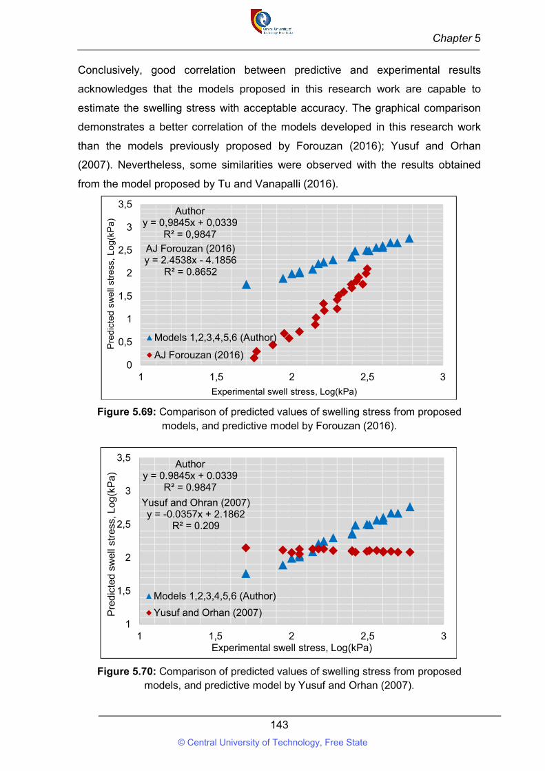
Chapter 5

143

Conclusively, good correlation between predictive and experimental results

acknowledges that the models proposed in this research work are capable to

estimate the swelling stress with acceptable accuracy. The graphical comparison

demonstrates a better correlation of the models developed in this research work

than the models previously proposed by Forouzan (2016); Yusuf and Orhan

(2007). Nevertheless, some similarities were observed with the results obtained

from the model proposed by Tu and Vanapalli (2016).

Figure 5.69: Comparison of predicted values of swelling stress from proposed models, and predictive model by Forouzan (2016).

Figure 5.70: Comparison of predicted values of swelling stress from proposed models, and predictive model by Yusuf and Orhan (2007).

Authory = 0,9845x + 0,0339

R² = 0,9847

AJ Forouzan (2016)y = 2.4538x - 4.1856

R² = 0.8652

0

0,5

1

1,5

2

2,5

3

3,5

1 1,5 2 2,5 3

Pre

dic

ted

sw

ell

stre

ss,

Log

(kP

a)

Experimental swell stress, Log(kPa)

Models 1,2,3,4,5,6 (Author)

AJ Forouzan (2016)

Author y = 0.9845x + 0.0339

R² = 0.9847

Yusuf and Ohran (2007)y = -0.0357x + 2.1862

R² = 0.209

1

1,5

2

2,5

3

3,5

1 1,5 2 2,5 3

Pre

dic

ted

sw

ell s

tres

s, L

og(k

Pa)



Yusuf and Orhan (2007)


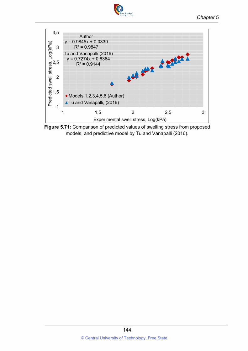
Chapter 5

144

Figure 5.71: Comparison of predicted values of swelling stress from proposed

models, and predictive model by Tu and Vanapalli (2016).

Author y = 0.9845x + 0.0339

R² = 0.9847

Tu and Vanapalli (2016)y = 0.7274x + 0.6364

R² = 0.9144

1

1,5

2

2,5

3

3,5

1 1,5 2 2,5 3

Pre

dic

ted

sw

ell s

tres

s, L

og(k

Pa)



Tu and Vanapalli, (2016)


Chapter 6

145

CHAPTER 6: CONCLUSION AND PERSPECTIVES

6.1 Summary

The main objective of this study was to characterize the relationship between the

swelling stress, the suction matric, and other soil parameters. Moreover, develop

models to predict the swelling stress of compacted expansive soils. To achieve

this aim, laboratory experiments such as particle size distribution, Atterberg limits,

linear shrinkage, free swell index, free swell ratio, specific gravity, X-ray diffraction,

modified Proctor compaction test, suction measurement, and zero-swell test (ZST)

were conducted to assess the physical and hydromechanical properties of soil

samples.

The data obtained from laboratory experiments were analyzed by multiple

regression analysis using software NCSS11. Correlations were established

between the swelling stress and the soil properties such as the matric suction, the

geotechnical index properties, and the expansive soil parameters. Moreover, six

mathematical models were proposed in this research work.

The validation of these models was conducted by comparing the predicted values

obtained from the proposed models and the predicted values obtained from other

existing models.

6.2 Conclusions

It was observed that, on the dry side of the OMC, there is an increase of the

swelling stress of field compacted expansive soils as the matric suction increases.

Nevertheless, the swelling stress reduces on the dry side of the OMC as the initial

water content, the initial dry density, and the linear shrinkage increases upon water

addition.

At the OMC, the swelling stress increases with the increment of plasticity index,

liquid limit, activity of clay, free swell ratio and free swell index. Besides, at the

OMC as the swelling stress values are within the range of 48.88 kPa to 261.81

kPa, and simultaneously, the matric suction values are within the range of 222.843

kPa to 1,778.27 kPa. The swelling stress values on the dry side of the OMC are

higher than the values on the wet side.


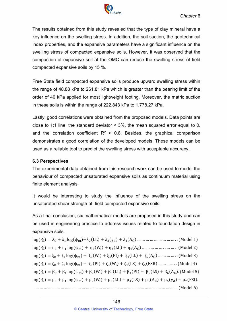
Chapter 6

146

The results obtained from this study revealed that the type of clay mineral have a

key influence on the swelling stress. In addition, the soil suction, the geotechnical

index properties, and the expansive parameters have a significant influence on the

swelling stress of compacted expansive soils. However, it was observed that the

compaction of expansive soil at the OMC can reduce the swelling stress of field

compacted expansive soils by 15 %.

Free State field compacted expansive soils produce upward swelling stress within

the range of 48.88 kPa to 261.81 kPa which is greater than the bearing limit of the

order of 40 kPa applied for most lightweight footing. Moreover, the matric suction

in these soils is within the range of 222.843 kPa to 1,778.27 kPa.

Lastly, good correlations were obtained from the proposed models. Data points are

close to 1:1 line, the standard deviator < 3%, the mean squared error equal to 0,

and the correlation coefficient R2 > 0.8. Besides, the graphical comparison

demonstrates a good correlation of the developed models. These models can be

used as a reliable tool to predict the swelling stress with acceptable accuracy.

6.3 Perspectives

The experimental data obtained from this research work can be used to model the

behaviour of compacted unsaturated expansive soils as continuum material using

finite element analysis.

It would be interesting to study the influence of the swelling stress on the

unsaturated shear strength of field compacted expansive soils.

As a final conclusion, six mathematical models are proposed in this study and can

be used in engineering practice to address issues related to foundation design in

expansive soils.

log (P ) = λ + λ log(ψ )+λ (LL) + λ (γ ) + λ (A ) … … … … … … … … … . . (Model 1)

log (P ) = η + η log(ψ ) + η (W ) + η (LL) + η (A ) … … … … … . . … … . . (Model 2)

log (P ) = ξ + ξ log(ψ ) + ξ (W ) + ξ (PI) + ξ (LL) + ξ (A ) … … … … . . (Model 3)

log (P ) = ζ + ζ log(ψ ) + ζ (PI) + ζ (W ) + ζ (LS) + ζ (FSR) … … . … . . . (Model 4)

log (P ) = β + β log(ψ ) + β (W ) + β (LL) + β (PI) + β (LS) + β (A ). (Model 5)

log (P ) = μ + μ log(ψ ) + μ (W ) + μ (LL) + μ (LS) + μ (A ) + μ (γ ) + μ (FSI).

… … … … … … … … … … … … … … … … … … … … … … … … … … … … … … … … … … (Model 6)


References

147

REFERENCES:

Abed, AA and Vermeer, PA. 2009. Numerical simulation of unsaturated soil

behaviour. International Journal of Computer Applications in

Technology, 34(1), pp 2-12.

Al-Rawas, AA and Goosen, MFeds. 2006. Expansive soils: recent advances in

characterization and treatment. Taylor & Francis.

ASTM, D. 2014. Standard test methods for one-dimensional swell or collapse of

soils. D4546-14.

ASTM, A. 2009. D6913−04 Standard test methods for particle-size distribution

(gradation) of soils using sieve analysis, ASTM Stand. Int.

ASTM, 2016. Standard test method for particle-size distribution (gradation) of fine-

grained soils using the sedimentation (hydrometer) analysis. D7928-16.

ASTM, 2005. ASTM D4318, standard test method for liquid limit, plastic limit, and

plasticity index of soils.

ASTM, D2010. Standard test methods for specific gravity of soil solids by water

pycnometer. D854.

ASTM, 1991. Standard test method for measurement of soil potential (suction)

using paper filter, ASTM D5298. Annual Book of ASTM Standards.

Atterberg, AM. 1911. Über die physikaliche Bodenuntersuchung und über die

Plastizität der Tone. Int. Mitt. Bodenkinde, 1.

Basma, AA., Al-Homoud, AS and Malkawi, AH. 1995. Laboratory assessment of

swelling pressure of expansive soils. Applied Clay Science, Vol.9, pp 355-

368.

Basu, R and Arulanandan, K. 1974. A new approach for the identification of swell

potential of soils. Bulletin of the Association of Engineering Geologists, 11:

pp 315-330.

BIS, I.1977. 2720 Methods of Test for Soils: Part 40 Determination of Free Swell

Index of Soils.


References

148

BRE. 1993. Low-rise buildings on shrinkable clay soils, RE Digests, pp 240-242.

Brindley, GW and Brown, G. 1984. Crystal Structures of Clay Minerals and Their

X-ray Diffraction Identification. London: Mineralogical Society. 495 p.

BS, 5930 .1981. Code of practice for site investigations. British Standard

Institution, London.

Cameron, RE and Van Ee, JJ. 1992. Guide to site and soil description for

hazardous waste site characterization: Metals. Environmental Monitoring

Systems Laboratory, Office of Research and Development, US

Environmental Protection Agency.

Cantillo, V., Mercado, V and Pájaro, C. 2017. Empirical Correlations for the

Swelling Pressure of Expansive Clays in the City of Barranquilla, Colombia.

Earth Sci. Res. J, 21(1).

Carter, M and Bentley, SP. 1991. Correlation of soil properties. Pentech Press,

London. Casagrande, A. (1932).

Chandler, RJ and Gutierrez, CI. 1986. The Filter Paper Method of Suction

Measurement”. Géotechnique 36 (2), pp 265-268.

Chen, FH. 1973. The basic physical property of expansive soils. Proc. of the 3rd

Int. Conf. on Expansive soils, Haifa, Israel, 1, pp 17-25.

Chleborad, AF., Diehl, SF and Cannon, SH. 2005. Geotechnical properties of

selected materials from the Slumgullion landslide.

Crilly, MS and Driscoll, RMC. 2000. The behaviour of lightly loaded piles in

swelling ground and implications for their design. Proceedings of the

Institution of Civil Engineers-Geotechnical Engineering, 143(1), pp 3-16.

Das, BM. 2002. Principles of geotechnical engineering, Thomson learning’s

California State University, Sacramento fifth edition. Ch2, pp 15-50.

Das, BM. 2008. Advanced Soil Mechanics. 3rd Ed., Taylor and Francis Group,

New York, USA.


References

149

Davies, JT and Rideal, EK. 1963. Interfacial Phenomena, 2nd ed., Academic, New

York, 584pp.

Deryagin, BV and Churaev, NV. 1987. Structure of water in thin

layers. Langmuir, 3(5), pp 607-612.

Department of Local Government, Housing and Works. 1990. Layman’s Guide to

Problem Soils, pp 37- 49.

Diop, S., Stapelberg, F., Tegegn, K., Ngubelanga, S and Heath, L. 2011. A review

on problem soils in south Africa. Council for Geoscience, 6, pp.1-48.

Dregne, HE. 1976. Soils of arid regions. American Elsevier Publishing Company

Inc, New York.

Elisha, AT. 2012. Prediction of Swell Pressure of Black Cotton Soil of North-

eastern Nigeria. Electronic Journal of Geotechnical Engineering, 17,

pp1731-1739.

Fattom, M and Barakat, S. 2000. Investigation of Three methods for Evaluating

Swelling pressure of Soils, Environmental & Engineering Geoscience 5(3),

pp 293-299.

Forouzan, AJ. 2016. Prediction of Swelling Behavior of Expansive Soils Using

Modified Free Swell Index, Methylene Bue and Swell Oedometer

Test. Middle East Technical University.

Fredlund, DG. 1979. Appropriate concepts and technology for unsaturated soils,

Second Canadian Geotechnical Colloquium, Canadian Geotechnical

Journal 16 (1), pp 121-139.

Fredlund, DG and Hasan, J. 1979. One-dimensional Consolidation Theory:

Unsaturated soils, Can. Geotech 16 (2), pp 521-531.

Fredlund, DG. 1987. The stress state for expansive soils. In proc. 6th int. conf.

Expansive soils, keynote Address, pp 1-9. December 1-3 New Delhi, India.

Fredlund, DG and Rahardjo, H. 1987. Soil mechanics principles for highway

engineering in Arid Regions. Transportation Res. Records 1137, pp 1-11.


References

150

Fredlund, DG and Rahardjo, H. 1993. Soil mechanics for unsaturated soils. John

Wiley & Sons, USA.

Fredlund, DG and Xing, A. 1994. Equation for soil-water characteristic curve,

Canadian Geotechnical Journal, 31 (3), pp 521-532.

Fredlund, DG and Morgenstern, NR. 1977. Stress state variables for unsaturated

soils. Journal of Geotechnical and Geoenvironmental Engineering, 103

(ASCE 12919).

Fredlund, DG., Rahardjo, H and Fredlund.MD. 2012. Unsaturated Soil Mechanics

in Engineering Practice. John Willey & Sons, Inc. ISBN: 978-1-118-13359-0

(Hardcopy). 926pp.

Fredlund, MD. 1994. The role of unsaturated soil property functions in the practice

of unsaturated soil mechanics. Ph.D. Dissertation, University of

Saskatchewan, Saskatoon, SK, Canada.

Fredlund, DG and Rahardjo, H. 1993. Soil Mechanics for Unsaturated Soils, John

Wiley & Sons, Inc, pp 1 - 77, 247 -258.

Fredlund, DG. 2000. The implementation of unsaturated soil mechanics into

geotechnical engineering, The R.M. Hardy Address, Canadian Geotechnical

Journal, 37(5), pp 963 - 986.

Gens, A., Alonso, EE and Lloret, A. 1995. Effect of structure on the volumetric

behaviour of a compacted soil. In Proceedings Of the first International

Conference on Unsaturated Soils / Unsat'95 / Paris / France / 6-8

September 1995. Volume 1.

Grim, RE. 1968. Clay Mineralogy McGraw-Hill. New York, p.206.

Houston, SL, Houston, WN and Wagner, A. 1994. Laboratory filter paper suction

measurements, Geotechnical Testing Journal, 17(2), pp185-194.

Holtz, WG, 1954. Engineering properties of expansive clays. Transactions of the

American Society of Civil Engineers , 121 , pp 641-677.


References

151

Holtz, RD., Kovacs, WD and Sheahan, TC. 1981. An introduction to geotechnical

engineering (Vol. 733). Englewood Cliffs, NJ: Prentice-Hall.

Israelachvili, JN. 1991. Intermolecular and Surface Forces, 2nd ed., Academic

press, New York.

Israr, J., Farooq, K and Mujtaba, HH. 2016. Modelling of swelling parameters and

associated characteristics based on index properties of expansive

soils. Pakistan Journal of Engineering and Applied Sciences.

Jennings, JEB and Knight, K. 1957. The predıctıon of total heave from the double

oedometer test, Proc. Symp. Expansive Clays. SAICE, Johannesburg, 7(9),

pp 13-19.

Jones, L.D. and Jefferson, I. 2012. Expansive soils.

Johnson, LT and Snethen, DR. 1978. Prediction of potential heave of swelling

soil. Geotechnical Testing Journal, 1(3), pp 117-124

Johnson, LD. 1973. Review of literature on expansive clay soils, US. Army Eng,

waterways Exp.sta. Vicksburg, Ms, Misc. Paper S, pp 73-17.

Jones, LD and Jefferson, I. 2012. Expansive soils. ICE Manual of Geotechnical

Engineering .Institution of civil Engineers, www.icemanuals.com; Ch 33, pp

413- 438.

Jones, LD. 1999. A Shrink/Swell classification for UK clay soils. Unpublished

B.Eng. Thesis. Nottingham Trent University, UK.

Johnson, RA. 2005. Miller and Freund’s probability and statistics for engineers.

Seventh edition, Prentice Hall, Englewood Cliffs, New Jersey.

Kaye, GWC and Laby, TH. 1973. Tables of Physical. Chemical Constants.

Kariuki, PC and Van Der Meer, F. 2004. A unified swelling potential index for

expansive soils. Engineering geology, 72(1-2), pp1-8.

Kassif, G and Baker, R. 1971. Aging effects on swell potential of compacted clay.

J.Soil Mechanics and Foundation Div., ASCE, SM 3: pp 529-540.


References

152

Katti, RK., Kulkarni, SK and Fotedar, SK. 1969. Shear strength and swelling

pressure characteristics of expansive soils. Proceeding of the second

International Research and Engineering Conference on expansive soils, pp

334-347. Texas.

Komornik, A and David, D. 1969. Prediction of swelling pressure of clays. J. Soil

Mech. Found. Div., Am. Soc. Civ. Eng.;(United States), 95.

Kyklema, J. 2000. Fundamentals of Interface and Colloid Science, Volume III,

Liquid-Fluid Interface, Academic, New York.

Lambe, TW and Whitman, RV. 1969. Soil mechanics. John Willey & Sons. Inc.,

New York, 553.

Lambe, TW and Whitman, RV. 1979. Soil Mechanics, Wiley, New York.

Lang, ARG. 1967. Osmotic coefficients and water potentials of sodium chloride

solutions from 0 to 40 C. Australian Journal of Chemistry, 20(9), pp 2017-

2023.

Leong, EC., He, L and Rahardjo, H. 2002. Factors affecting the filter paper method

for total and matric suction measurements. Geotechnical Testing

Journal, 25(3), pp 322-333.

Ling, NL and Toll, DG. 2000. Suction and Strength Behaviour of Unsaturated

Calcrete, Unsaturated Soils for Asia, Rahardjo, Toll & Leong (Eds), pp 533-

538.

Meigs, P. 1953. World distributions of arid and semi-arid homoclimates, in Review

of research on arid zone hydrology. Arid zone program, 1,, pp 203-209.

Mitchell, JK. 1976. Fundamentals of soil behaviour, John Willy, New York.

Mitchell, JK. 1979. In situ techniques for site characterization, Proc. of ASCE

Specially Workshop Site Charact. Exp., Evanston, pp 107-129.

Mitchell, J.K. 1993. Fundamentals of soil behavior (No. Ed. 2). John Wiley and

Sons, Inc.


References

153

Murray, HH. 2007. Occurrences, processing and application of kaolins, bentonites,

palygorskite-sepiolite, and common clays. Applied Clay Mineralogy.

Elsevier, Amsterdam.

Murthy, VNS. 2002. Geotechnical engineering: principles and practices of soil

mechanics and foundation engineering. CRC press.

Nelson, JD and Miller, DJ. 1992. Expansive Soils: Problems and Practice in

Foundation and Pavement Engineering. John Wiley & Sons, Inc., New York.

Nelson, JD., Overton, DD and Durkee, DB. 2001. Depth of wetting and the active

zone. Expansive clay soils and vegetative influence on shallow foundations,

ASCE Geotechnical special publications No.116,p 95-109.

Odom, IE. 1984. Smectite clay minerals: properties and uses. Philosophical

Transactions of the Royal Society of London. Series A, Mathematical and

Physical Sciences, 311(1517), pp.391-409.

Oloo, S., Schreiner, HD and Burland, JB., 1987.Identification and classification of

expansive soils. In 6th International Conference on Expansive Soils, pp. 23-

29.

Oweis, I and Khera. 1998. “Geotechnology of Waste Management’’.

Patel, AD., Stamatakis, E., Davis, E and Friedheim, J. 2007.High Performance

Water Based Drilling Fluids and Method of Used, Houston.

Rank, K, Bhanderi, J and Nagecha, K .2015. Swelling potential of different

expansive soil placed at different dry density and initial water content,

IJAERD 2 (3).

Rao, AS., Phanikumar, BR and Sharma, RS. 2004. Prediction of swelling

characteristics of remoulded and compacted expansive soils using free

swell index. Quarterly Journal of Engineering Geology and

Hydrogeology, 37(3), pp 217-226.


References

154

Reeve, MJ., Hall, DGM and Bullock, P.1980. The effect of soil composition and

environmental factors on the shrinkage of some clayey British soils. Journal

of Soil Science, 31(3), pp 429-442.

Sachan, A and Penumadu, D. 2007. Effect of microfabric on shear behavior of

kaolin clay. Journal of geotechnical and geoenvironmental

engineering, 133(3), pp 306-318.

Seki, K. 2007. SWRC fit–a nonlinear fitting program with a water retention curve

for soils having unimodal and bimodal pore structure. Hydrology and Earth

System Sciences Discussions, 4(1), pp 407-437.

Seed, HB., Mitchell, JK and Chan, CK. 1960. The strength of compacted

cohesive soils. Proceedings, ASCE Research Conference on Cohesive

soils,

Boulder, American Society of Civil Engineers, New York, pp 877-964.

Sillers, WS and Fredlund, DG. 2001. Statistical assessment of soil-water

characteristic curve models for geotechnical engineering. Canadian

Geotechnical Journal, 38(6),pp 1297-1313.

Sibley, JW., Smyth, GK and Williams, DJ. 1990. Suction-moisture content

calibration of filter papers from different boxes. Geotechnical Testing

Journal, 13(3), pp 257-262.

Skempton, AW. 1953. The colloidal activity of clays. Selected papers on soil

mechanics, pp 106-118.

Sorochan, EA. 1991. Construction of buildings on expansile soils, A.A.

Balkema/Rotterdam/Brookfield, pp 5-6.

Sridharan, A and Prakash, K. 1998. Characteristic water contents of a fine-grained

soil-water system. Geotechnique, 48(3), pp 337-346.

Sridharan, A., Prakash K .1998b. Mechanism controlling the shrinkage limit of

soils. Geotech Test J ASTM 21(3), pp 240-250.


References

155

Sridharan, A and Prakash, K. 2000. Classification procedures for expansive soils.

Geotech.Eng, 143, pp 235-240.

Sridharan, A, Rao, SM and Murthy, NS. 1985. Free Swell Index of Soils: A Need

for Redefinition. Indian Geotechnical Journal, 15(2), pp 94-99.

Swarbrick, GE. 1995. Measurement of Soil Suction Using the Filter Paper

Method.1st Int. Conf. on Unsaturated Soils, Paris paper No: 246.

Thakur, VKS and Singh, DN. 2005. Swelling and suction in clay

minerals. Advanced Experimental Unsaturated Soil Mechanics, pp 27–31.

TMH1 A7. 1986. Standard Methods of Testing Road Construction Materials.

Technical Methods for Highways. The determination of the maximum dry

density and optimum moisture content of gravel, soil and sand. Committee

of State Road Authorities. Pretoria.

Tu, H and Vanapalli, SK. 2016. Prediction of the variation of swelling pressure and

one-dimensional heave of expansive soils with respect to suction using the

soil-water retention curve as a tool. Canadian Geotechnical Journal, 53(8),

pp1213-1234.

Vanapalli, SK., Fredlund, DG and Pufahl, DE. 1999. The influence of soil structure

and stress history on the soil-water characteristics of a compacted till.

Géotechnique 49(2): pp 143–159.

Van Genuchten, MT.1980. A closed-form equation for predicting the hydraulic

conductivity of unsaturated soils 1. Soil science society of America

journal, 44(5), pp.892-898.

Van der Merwe, DH. 1964. The prediction of heave from the plasticity index and

percentage clay fraction of soils. Civil Engineering=Siviele

Ingenieurswese, 1964(v6i6), pp 103-107.

Wang, YH and Fredlund, DG. 2003. Towards a better understanding of the role of

the contractile skin, Proceedings of the Second Asian Conference on

Unsaturated Soils, UNSAT-ASIA, Osaka, pp 419-424.


References

156

Williams, AAB. 1958. Discussion of the prediction of total heave from double

oedometer test. Transactions, South African Institution of Civil

Engineers, 5(6), pp 49-51.

Williams, AAB., Pidgeon, JT and Day, PW. 1985. Expansive soils. Civil

Engineering= Siviele Ingenieurswese, 27(7), pp 367-377.

Wu, FT. 1978. Mineralogy and physical nature of clay gouge. pure and applied

geophysics, 116 (4-5), pp 655-689.

YA, Tan .2016. Swelling Pressure and Retaining Wall Design in Expansive Soils.

MScThesis, RMIT University, Melbourne.Australia.

Yusuf, E and Orhan, E. 2007. Swell pressure prediction by suction methods.

Engineering Geology 92, pp 133-145.

Zha, FS., Liu, SY and Du, YJ. 2006. Evaluation of swell-shrinkage properties of

compacted expansive soils using electrical resistivity method.

In Proceedings of the Sessions of GeoShanghai: Advances in Unsaturated

Soil, Seepage, and Environmental Geotechnics, pp 143-151.


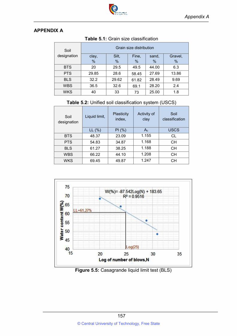
Appendix A

157

APPENDIX A

Table 5.1: Grain size classification

Soil designation

Grain size distribution

clay, %

Silt, %

Fine, %

sand, %

Gravel, %

BTS 20 29.5 49.5 44.00 6.3

PTS 29.85 28.6 58.45 27.69 13.86

BLS 32.2 29.62 61.82 28.49 9.69

WBS 36.5 32.6 69.1 28.20 2.4

WKS 40 33 73 25.00 1.8

Table 5.2: Unified soil classification system (USCS)

Soil designation

Liquid limit,

Plasticity

index,

Activity of

clay

Soil

classification

LL (%) PI (%) Ac USCS

BTS 48.37 23.09 1.155 CL

PTS 54.83 34.87 1.168 CH

BLS 61.27 38.25 1.188 CH

WBS 66.22 44.10 1.208 CH

WKS 69.45 49.87 1.247 CH

Figure 5.5: Casagrande liquid limit test (BLS)


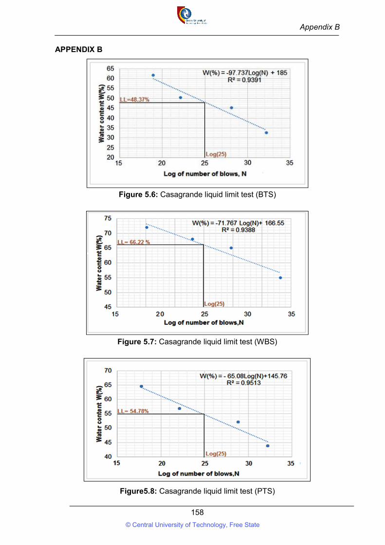
Appendix B

158

APPENDIX B

Figure 5.6: Casagrande liquid limit test (BTS)

Figure 5.7: Casagrande liquid limit test (WBS)

Figure5.8: Casagrande liquid limit test (PTS)


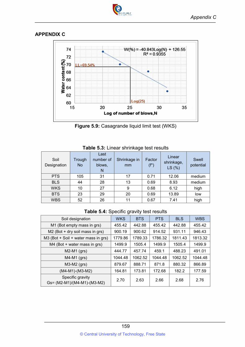
Appendix C

159

APPENDIX C

Figure 5.9: Casagrande liquid limit test (WKS)

Table 5.3: Linear shrinkage test results

Soil Designation

Trough No

Last number of

blows, N

Shrinkage in mm

Factor (f*)

Linear shrinkage,

LS (%)

Swell potential

PTS 105 31 17 0.71 12.06 medium

BLS 44 28 13 0.69 8.93 medium

WKS 10 27 9 0.68 6.12 high

BTS 23 29 20 0.69 13.89 low

WBS 52 26 11 0.67 7.41 high

Table 5.4: Specific gravity test results

Soil designation WKS BTS PTS BLS WBS

M1 (Bot empty mass in grs) 455.42 442.88 455.42 442.88 455.42

M2 (Bot + dry soil mass in grs) 900.19 900.62 914.52 931.11 946.43

M3 (Bot + Soil + water mass in grs) 1779.86 1789.33 1786.32 1811.43 1813.32

M4 (Bot + water mass in grs) 1499.9 1505.4 1499.9 1505.4 1499.9

M2-M1 (grs) 444.77 457.74 459.1 488.23 491.01

M4-M1 (grs) 1044.48 1062.52 1044.48 1062.52 1044.48

M3-M2 (grs) 879.67 888.71 871.8 880.32 866.89

(M4-M1)-(M3-M2) 164.81 173.81 172.68 182.2 177.59

Specific gravity Gs= (M2-M1)/(M4-M1)-(M3-M2)

2.70 2.63 2.66 2.68 2.76


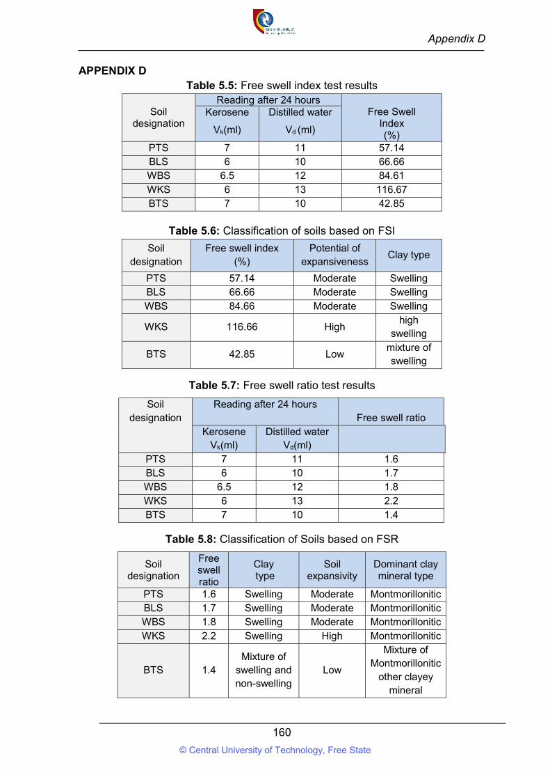
Appendix D

160

APPENDIX D Table 5.5: Free swell index test results

Soil

designation

Reading after 24 hours Free Swell

Index (%)

Kerosene

Vk(ml)

Distilled water

Vd (ml)

PTS 7 11 57.14 BLS 6 10 66.66 WBS 6.5 12 84.61 WKS 6 13 116.67 BTS 7 10 42.85

Table 5.6: Classification of soils based on FSI

Soil designation

Free swell index (%)

Potential of expansiveness

Clay type

PTS 57.14 Moderate Swelling BLS 66.66 Moderate Swelling WBS 84.66 Moderate Swelling

WKS 116.66 High high

swelling

BTS 42.85 Low mixture of swelling

Table 5.7: Free swell ratio test results

Soil designation

Reading after 24 hours Free swell ratio

Kerosene Vk(ml)

Distilled water Vd(ml)

PTS 7 11 1.6 BLS 6 10 1.7 WBS 6.5 12 1.8 WKS 6 13 2.2 BTS 7 10 1.4

Table 5.8: Classification of Soils based on FSR

Soil designation

Free swell ratio

Clay type

Soil expansivity

Dominant clay mineral type

PTS 1.6 Swelling Moderate Montmorillonitic BLS 1.7 Swelling Moderate Montmorillonitic WBS 1.8 Swelling Moderate Montmorillonitic WKS 2.2 Swelling High Montmorillonitic

BTS 1.4 Mixture of

swelling and non-swelling

Low

Mixture of Montmorillonitic

other clayey mineral


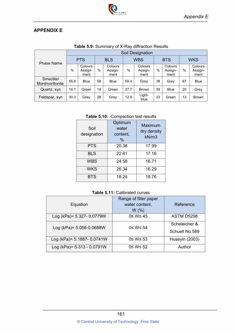
Appendix E

161

APPENDIX E

Table 5.9: Summary of X-Ray diffraction Results

Phase Name

Soil Designation

PTS BLS WBS BTS WKS

% Colours Assign-

ment %

Colours Assign-

ment %

Colours Assign-ment

% Colours Assign-ment

% Colours Assign-ment

Smectite/ Montmorillonite

55.6 Blue 58 Blue 59.4 Grey 38 Grey 67 Blue

Quartz, syn 14.1 Green 14 Green 27.7 Brown 39 Blue 20 Grey

Feldspar, syn 30.3 Grey 28 Grey 12.9 Light-blue

23 Green 13 Brown

Table 5.10: Compaction test results

Soil designation

Optimum water

content, %

Maximum dry density

kN/m3

PTS 20.38 17.99

BLS 22.61 17.16

WBS 24.58 16.71

WKS 26.34 16.29

BTS 18.24 18.76

Table 5.11: Calibrated curves

Equation Range of filter paper

water content, W (%)

Reference

Log (kPa)= 5.327- 0.0779W 0≤ W≤ 45 ASTM D5298

Log (kPa)= 5.056-0.0688W 0≤ W≤ 54 Scheleicher &

Schuell No.589

Log (kPa)= 5.1887- 0.0741W 0≤ W≤ 53 Huseyin (2003)

Log (kPa)= 5.313 - 0.0791W 0≤ W≤ 52 Author


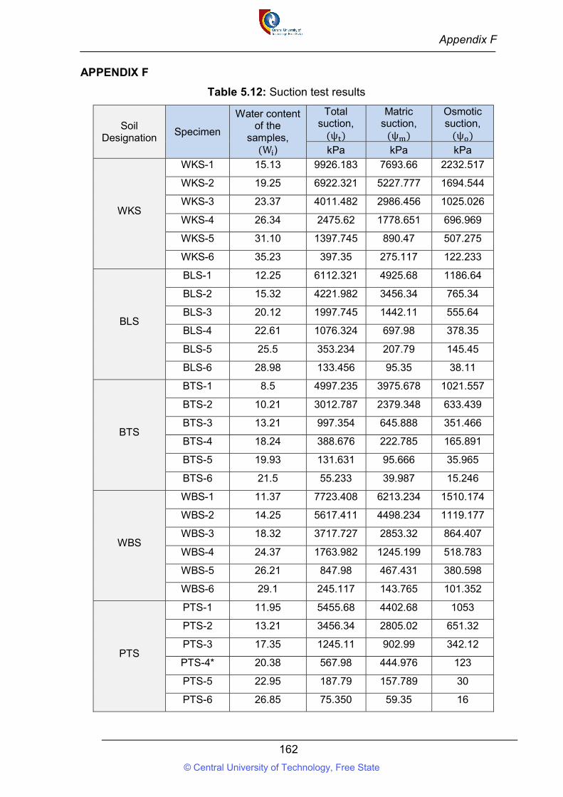
Appendix F

162

APPENDIX F

Table 5.12: Suction test results

Soil Designation

Specimen

Water content of the

samples, (W )

Total suction,

(ψ )

Matric suction,

(ψ )

Osmotic suction,

(ψ ) kPa kPa kPa

WKS

WKS-1 15.13 9926.183 7693.66 2232.517

WKS-2 19.25 6922.321 5227.777 1694.544

WKS-3 23.37 4011.482 2986.456 1025.026

WKS-4 26.34 2475.62 1778.651 696.969

WKS-5 31.10 1397.745 890.47 507.275

WKS-6 35.23 397.35 275.117 122.233

BLS

BLS-1 12.25 6112.321 4925.68 1186.64

BLS-2 15.32 4221.982 3456.34 765.34

BLS-3 20.12 1997.745 1442.11 555.64

BLS-4 22.61 1076.324 697.98 378.35

BLS-5 25.5 353.234 207.79 145.45

BLS-6 28.98 133.456 95.35 38.11

BTS

BTS-1 8.5 4997.235 3975.678 1021.557

BTS-2 10.21 3012.787 2379.348 633.439

BTS-3 13.21 997.354 645.888 351.466

BTS-4 18.24 388.676 222.785 165.891

BTS-5 19.93 131.631 95.666 35.965

BTS-6 21.5 55.233 39.987 15.246

WBS

WBS-1 11.37 7723.408 6213.234 1510.174

WBS-2 14.25 5617.411 4498.234 1119.177

WBS-3 18.32 3717.727 2853.32 864.407

WBS-4 24.37 1763.982 1245.199 518.783

WBS-5 26.21 847.98 467.431 380.598

WBS-6 29.1 245.117 143.765 101.352

PTS

PTS-1 11.95 5455.68 4402.68 1053

PTS-2 13.21 3456.34 2805.02 651.32

PTS-3 17.35 1245.11 902.99 342.12

PTS-4* 20.38 567.98 444.976 123

PTS-5 22.95 187.79 157.789 30

PTS-6 26.85 75.350 59.35 16


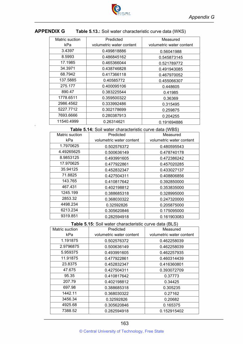
Appendix G

163

APPENDIX G Table 5.13.: Soil water characteristic curve data (WKS)

Matric suction kPa

Predicted volumetric water content

Measured volumetric water content

3.4397 0.499818886 0.56041988 8.5993 0.486845162 0.545873145

17.1985 0.465366044 0.521789772 34.3971 0.438746828 0.491943085 68.7942 0.417366118 0.467970052

137.5885 0.40585772 0.455066307 275.177 0.400095106 0.448605 890.47 0.383225544 0.41985

1778.6511 0.359500322 0.36369 2986.4562 0.333992486 0.315495 5227.7712 0.302178699 0.259875 7693.6666 0.280387913 0.204255

11540.4999 0.26314621 0.191694886 3

Table 5.14: Soil water characteristic curve data (WBS) Matric suction

kPa Predicted

volumetric water content Measured

volumetric water content

1.7970625 0.502576372 0.480595543 4.49265625 0.500636149 0.478740178 8.9853125 0.493991605 0.472386242 17.970625 0.477922861 0.457020285 35.94125 0.452832347 0.433027137 71.8825 0.427504311 0.408806856 143.765 0.410817642 0.392850000 467.431 0.402198812 0.353835000

1245.199 0.388685318 0.328995000 2853.32 0.368030322 0.247320000

4498.234 0.32592826 0.205875000 6213.234 0.305620846 0.175095000 9319.851 0.282594918 0.161903083

Table 5.15: Soil water characteristic curve data (BLS) Matric suction

kPa Predicted

volumetric water content Measured

volumetric water content

1.191875 0.502576372 0.462258039 2.9796875 0.500636149 0.462258039 5.959375 0.493991605 0.462257935 11.91875 0.477922861 0.460314439 23.8375 0.452832347 0.416360801 47.675 0.427504311 0.393072709 95.35 0.410817642 0.37773

207.79 0.402198812 0.34425 697.98 0.388685318 0.305235

1442.11 0.368030322 0.27162 3456.34 0.32592826 0.20682 4925.68 0.305620846 0.165375 7388.52 0.282594918 0.152915402


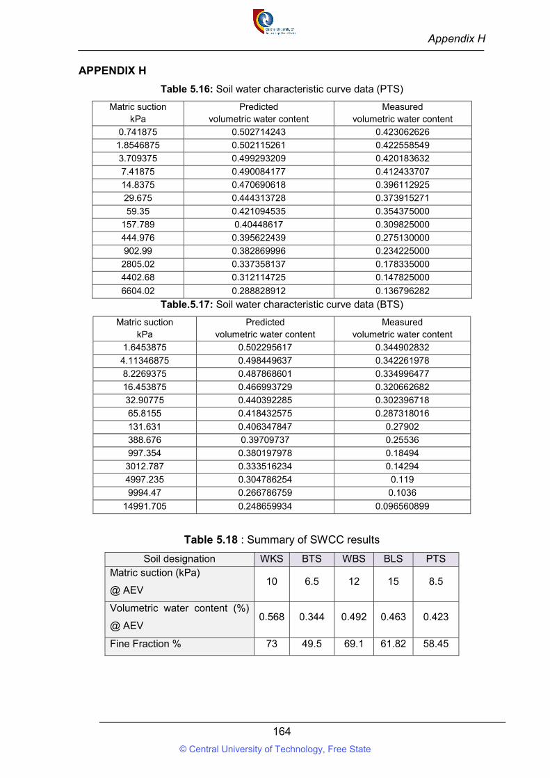
Appendix H

164

APPENDIX H

Table 5.16: Soil water characteristic curve data (PTS)

Matric suction kPa



0.741875 0.502714243 0.423062626

1.8546875 0.502115261 0.422558549

3.709375 0.499293209 0.420183632

7.41875 0.490084177 0.412433707

14.8375 0.470690618 0.396112925

29.675 0.444313728 0.373915271

59.35 0.421094535 0.354375000

157.789 0.40448617 0.309825000

444.976 0.395622439 0.275130000

902.99 0.382869996 0.234225000

2805.02 0.337358137 0.178335000

4402.68 0.312114725 0.147825000

6604.02 0.288828912 0.136796282

Table.5.17: Soil water characteristic curve data (BTS)

Matric suction kPa



1.6453875 0.502295617 0.344902832

4.11346875 0.498449637 0.342261978

8.2269375 0.487868601 0.334996477

16.453875 0.466993729 0.320662682

32.90775 0.440392285 0.302396718

65.8155 0.418432575 0.287318016

131.631 0.406347847 0.27902

388.676 0.39709737 0.25536

997.354 0.380197978 0.18494

3012.787 0.333516234 0.14294

4997.235 0.304786254 0.119

9994.47 0.266786759 0.1036

14991.705 0.248659934 0.096560899

Table 5.18 : Summary of SWCC results

Soil designation WKS BTS WBS BLS PTS Matric suction (kPa)

@ AEV 10 6.5 12 15 8.5

Volumetric water content (%)

@ AEV 0.568 0.344 0.492 0.463 0.423

Fine Fraction % 73 49.5 69.1 61.82 58.45


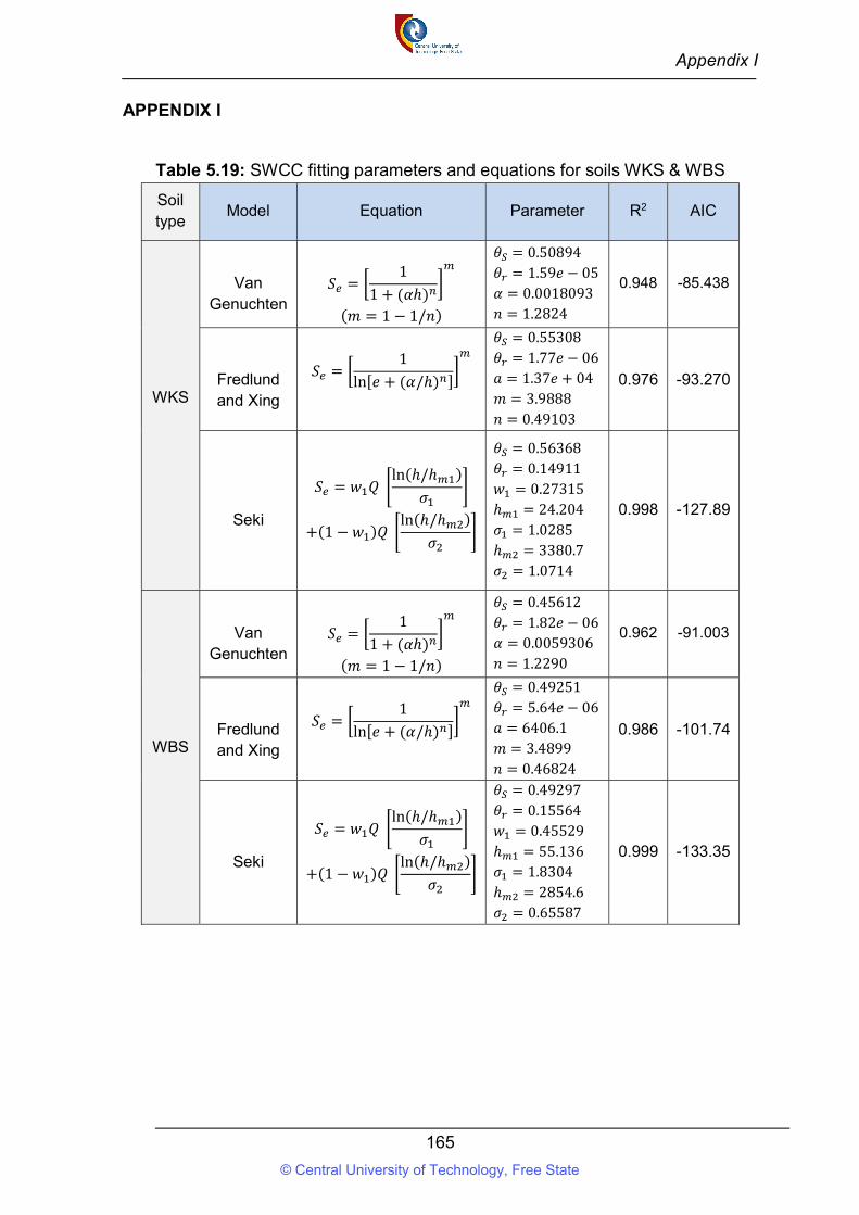
Appendix I

165

APPENDIX I

Table 5.19: SWCC fitting parameters and equations for soils WKS & WBS

Soil type

Model Equation Parameter R2 AIC

WKS

Van

Genuchten

𝑆 =1

1 + (𝛼ℎ)

(𝑚 = 1 − 1/𝑛)

𝜃 = 0.50894 𝜃 = 1.59𝑒 − 05 𝛼 = 0.0018093 𝑛 = 1.2824

0.948 -85.438

Fredlund and Xing

𝑆 =1

ln[𝑒 + (𝛼/ℎ) ]

𝜃 = 0.55308 𝜃 = 1.77𝑒 − 06 𝑎 = 1.37𝑒 + 04 𝑚 = 3.9888 𝑛 = 0.49103

0.976

-93.270

Seki

𝑆 = 𝑤 𝑄 ln(ℎ/ℎ )

𝜎

+(1 − 𝑤 )𝑄 ln(ℎ/ℎ )

𝜎

𝜃 = 0.56368 𝜃 = 0.14911 𝑤 = 0.27315 ℎ = 24.204 𝜎 = 1.0285 ℎ = 3380.7 𝜎 = 1.0714

0.998 -127.89

WBS

Van

Genuchten

𝑆 =1

1 + (𝛼ℎ)

(𝑚 = 1 − 1/𝑛)

𝜃 = 0.45612 𝜃 = 1.82𝑒 − 06 𝛼 = 0.0059306 𝑛 = 1.2290

0.962 -91.003

Fredlund and Xing

𝑆 =1

ln[𝑒 + (𝛼/ℎ) ]

𝜃 = 0.49251 𝜃 = 5.64𝑒 − 06 𝑎 = 6406.1 𝑚 = 3.4899 𝑛 = 0.46824

0.986

-101.74

Seki


𝜎

+(1 − 𝑤 )𝑄 ln(ℎ/ℎ )

𝜎

𝜃 = 0.49297 𝜃 = 0.15564 𝑤 = 0.45529 ℎ = 55.136 𝜎 = 1.8304 ℎ = 2854.6 𝜎 = 0.65587

0.999 -133.35


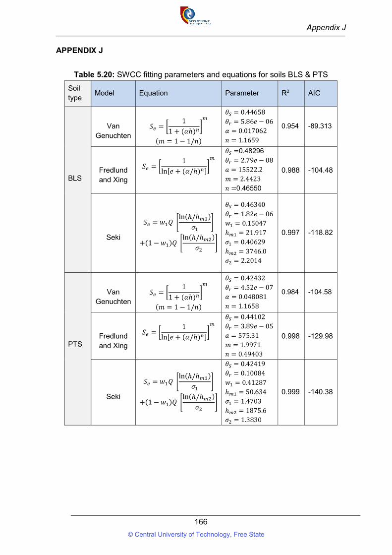
Appendix J

166

APPENDIX J

Table 5.20: SWCC fitting parameters and equations for soils BLS & PTS

Soil type


BLS

Van

Genuchten

𝑆 =1

1 + (𝛼ℎ)

(𝑚 = 1 − 1/𝑛)

𝜃 = 0.44658 𝜃 = 5.86𝑒 − 06 𝛼 = 0.017062 𝑛 = 1.1659

0.954 -89.313

Fredlund and Xing

𝑆 =1

ln[𝑒 + (𝛼/ℎ) ]

𝜃 =0.48296 𝜃 = 2.79𝑒 − 08 𝑎 = 15522.2 𝑚 = 2.4423 𝑛 =0.46550

0.988

-104.48

Seki


𝜎

+(1 − 𝑤 )𝑄 ln(ℎ/ℎ )

𝜎

𝜃 = 0.46340 𝜃 = 1.82𝑒 − 06 𝑤 = 0.15047 ℎ = 21.917 𝜎 = 0.40629 ℎ = 3746.0 𝜎 = 2.2014

0.997 -118.82

PTS

Van

Genuchten

𝑆 =1

1 + (𝛼ℎ)

(𝑚 = 1 − 1/𝑛)

𝜃 = 0.42432 𝜃 = 4.52𝑒 − 07 𝛼 = 0.048081 𝑛 = 1.1658

0.984 -104.58

Fredlund and Xing

𝑆 =1

ln[𝑒 + (𝛼/ℎ) ]

𝜃 = 0.44102 𝜃 = 3.89𝑒 − 05 𝑎 = 575.31 𝑚 = 1.9971 𝑛 = 0.49403

0.998

-129.98

Seki


𝜎

+(1 − 𝑤 )𝑄 ln(ℎ/ℎ )

𝜎

𝜃 = 0.42419 𝜃 = 0.10084 𝑤 = 0.41287 ℎ = 50.634 𝜎 = 1.4703 ℎ = 1875.6 𝜎 = 1.3830

0.999 -140.38


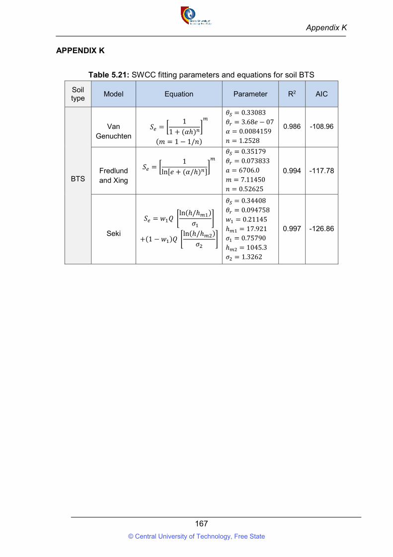
Appendix K

167

APPENDIX K

Table 5.21: SWCC fitting parameters and equations for soil BTS

Soil type


BTS

Van Genuchten

𝑆 =1

1 + (𝛼ℎ)

(𝑚 = 1 − 1/𝑛)

𝜃 = 0.33083 𝜃 = 3.68𝑒 − 07 𝛼 = 0.0084159 𝑛 = 1.2528

0.986 -108.96

Fredlund and Xing

𝑆 =1

ln[𝑒 + (𝛼/ℎ) ]

𝜃 = 0.35179 𝜃 = 0.073833 𝑎 = 6706.0 𝑚 = 7.11450 𝑛 = 0.52625

0.994 -117.78

Seki


𝜎

+(1 − 𝑤 )𝑄 ln(ℎ/ℎ )

𝜎

𝜃 = 0.34408 𝜃 = 0.094758 𝑤 = 0.21145 ℎ = 17.921 𝜎 = 0.75790 ℎ = 1045.3 𝜎 = 1.3262

0.997 -126.86


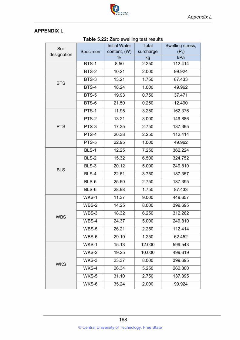
Appendix L

168

APPENDIX L

Table 5.22: Zero swelling test results

Soil designation

Specimen Initial Water content, (W)

Total surcharge

Swelling stress, (Ps)

% kg kPa

BTS

BTS-1 8.50 2.250 112.414

BTS-2 10.21 2.000 99.924

BTS-3 13.21 1.750 87.433

BTS-4 18.24 1.000 49.962

BTS-5 19.93 0.750 37.471

BTS-6 21.50 0.250 12.490

PTS

PTS-1 11.95 3.250 162.376

PTS-2 13.21 3.000 149.886

PTS-3 17.35 2.750 137.395

PTS-4 20.38 2.250 112.414

PTS-5 22.95 1.000 49.962

BLS

BLS-1 12.25 7.250 362.224

BLS-2 15.32 6.500 324.752

BLS-3 20.12 5.000 249.810

BLS-4 22.61 3.750 187.357

BLS-5 25.50 2.750 137.395

BLS-6 28.98 1.750 87.433

WBS

WKS-1 11.37 9.000 449.657

WBS-2 14.25 8.000 399.695

WBS-3 18.32 6.250 312.262

WBS-4 24.37 5.000 249.810

WBS-5 26.21 2.250 112.414

WBS-6 29.10 1.250 62.452

WKS

WKS-1 15.13 12.000 599.543

WKS-2 19.25 10.000 499.619

WKS-3 23.37 8.000 399.695

WKS-4 26.34 5.250 262.300

WKS-5 31.10 2.750 137.395

WKS-6 35.24 2.000 99.924


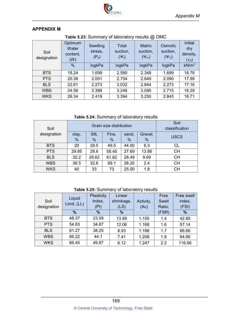
Appendix M

169

APPENDIX M

Table 5.23: Summary of laboratory results @ OMC

Soil designation

Optimum Water

content, (W)

Swelling stress,

(Ps)

Total suction,

(Ψt)

Matric suction,

(Ψm)

Osmotic suction,

(ΨO)

Initial dry

density, (γd)

% logkPa logkPa logkPa logkPa kN/m3

BTS 18.24 1.699 2.590 2.348 1.699 18.76

PTS 20.38 2.051 2.754 2.649 2.090 17.99

BLS 22.61 2.273 3.032 2.844 2.273 17.16

WBS 24.58 2.398 3.246 3.095 2.715 16.29

WKS 26.34 2.419 3.394 3.250 2.843 16.71

Table 5.24: Summary of laboratory results

Soil designation

Grain size distribution Soil

classification clay,

% Silt, %

Fine, %

sand, %

Gravel, %

USCS

BTS 20 29.5 49.5 44.00 6.3 CL

PTS 29.85 28.6 58.45 27.69 13.86 CH

BLS 32.2 29.62 61.82 28.49 9.69 CH

WBS 36.5 32.6 69.1 28.20 2.4 CH

WKS 40 33 73 25.00 1.8 CH

Table 5.25: Summary of laboratory results

Soil designation

Liquid Limit, (LL)

Plasticity Index,

(PI)

Linear shrinkage,

(LS) Activity,

(Ac)

Free Swell Ratio, (FSR)

Free swell index, (FSI)

% % % %

BTS 48.37 23.09 13.89 1.155 1.4 42.85

PTS 54.83 34.87 12.06 1.168 1.6 57.14

BLS 61.27 38.25 8.93 1.188 1.7 66.66

WBS 66.22 44.1 7.41 1.208 1.8 84.66

WKS 69.45 49.87 6.12 1.247 2.2 116.66


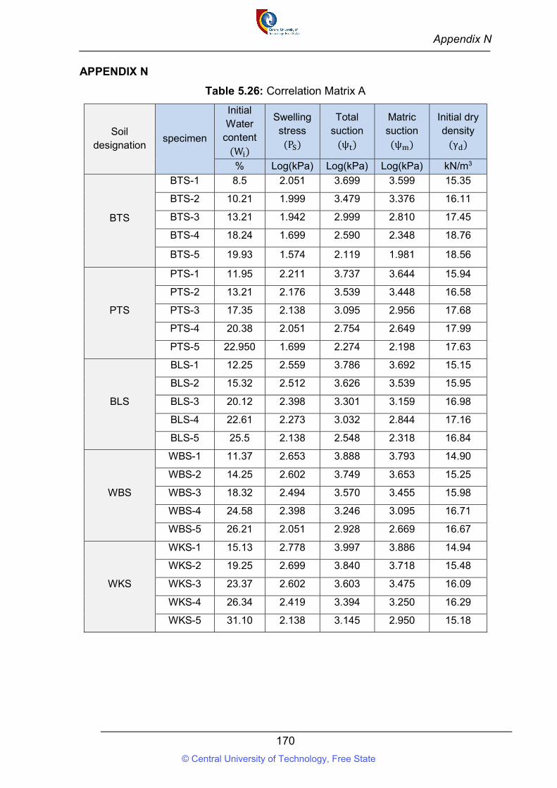
Appendix N

170

APPENDIX N

Table 5.26: Correlation Matrix A

Soil designation

specimen

Initial Water

content (W )

Swelling stress

(P )

Total suction

(ψ )

Matric suction

(ψ )

Initial dry density

(γ )

% Log(kPa) Log(kPa) Log(kPa) kN/m3

BTS

BTS-1 8.5 2.051 3.699 3.599 15.35

BTS-2 10.21 1.999 3.479 3.376 16.11

BTS-3 13.21 1.942 2.999 2.810 17.45

BTS-4 18.24 1.699 2.590 2.348 18.76

BTS-5 19.93 1.574 2.119 1.981 18.56

PTS

PTS-1 11.95 2.211 3.737 3.644 15.94

PTS-2 13.21 2.176 3.539 3.448 16.58

PTS-3 17.35 2.138 3.095 2.956 17.68

PTS-4 20.38 2.051 2.754 2.649 17.99

PTS-5 22.950 1.699 2.274 2.198 17.63

BLS

BLS-1 12.25 2.559 3.786 3.692 15.15

BLS-2 15.32 2.512 3.626 3.539 15.95

BLS-3 20.12 2.398 3.301 3.159 16.98

BLS-4 22.61 2.273 3.032 2.844 17.16

BLS-5 25.5 2.138 2.548 2.318 16.84

WBS

WBS-1 11.37 2.653 3.888 3.793 14.90

WBS-2 14.25 2.602 3.749 3.653 15.25

WBS-3 18.32 2.494 3.570 3.455 15.98

WBS-4 24.58 2.398 3.246 3.095 16.71

WBS-5 26.21 2.051 2.928 2.669 16.67

WKS

WKS-1 15.13 2.778 3.997 3.886 14.94

WKS-2 19.25 2.699 3.840 3.718 15.48

WKS-3 23.37 2.602 3.603 3.475 16.09

WKS-4 26.34 2.419 3.394 3.250 16.29

WKS-5 31.10 2.138 3.145 2.950 15.18


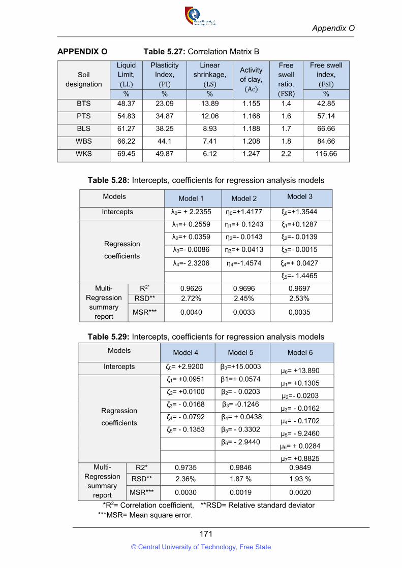
Appendix O

171

APPENDIX O Table 5.27: Correlation Matrix B

Soil designation

Liquid Limit, (LL)

Plasticity Index,

(PI)

Linear shrinkage,

(LS)

Activity of clay,

(Ac)

Free swell ratio, (FSR)

Free swell index, (FSI)

% % % % BTS 48.37 23.09 13.89 1.155 1.4 42.85

PTS 54.83 34.87 12.06 1.168 1.6 57.14

BLS 61.27 38.25 8.93 1.188 1.7 66.66

WBS 66.22 44.1 7.41 1.208 1.8 84.66

WKS 69.45 49.87 6.12 1.247 2.2 116.66

Table 5.28: Intercepts, coefficients for regression analysis models

Models Model 1 Model 2 Model 3

Intercepts λ0= + 2.2355 η0=+1.4177 ξ0=+1.3544

Regression

coefficients

λ1=+ 0.2559 η1=+ 0.1243 ξ1=+0.1287

λ2=+ 0.0359 η2=- 0.0143 ξ2=- 0.0139

λ3=- 0.0086 η3=+ 0.0413 ξ3=- 0.0015

λ4=- 2.3206 η4=-1.4574 ξ4=+ 0.0427

ξ5=- 1.4465

Multi-Regression summary

report

R2* 0.9626 0.9696 0.9697 RSD** 2.72% 2.45% 2.53%

MSR*** 0.0040 0.0033 0.0035

Table 5.29: Intercepts, coefficients for regression analysis models

Models Model 4 Model 5 Model 6

Intercepts ζ0= +2.9200 β0=+15.0003 μ0= +13.890

Regression

coefficients

ζ1= +0.0951 β1=+ 0.0574 μ1= +0.1305

ζ2= +0.0100 β2= - 0.0203 μ2=- 0.0203

ζ3= - 0.0168 β3= -0.1246 μ3= - 0.0162

ζ4= - 0.0792 β4= + 0.0438 μ4= - 0.1702

ζ5= - 0.1353 β5= - 0.3302 μ5= - 9.2460

β6= - 2.9440 μ6= + 0.0284

μ7= +0.8825 Multi-

Regression summary

report

R2* 0.9735 0.9846 0.9849

RSD** 2.36% 1.87 % 1.93 %

MSR*** 0.0030 0.0019 0.0020

*R2= Correlation coefficient, **RSD= Relative standard deviator ***MSR= Mean square error.


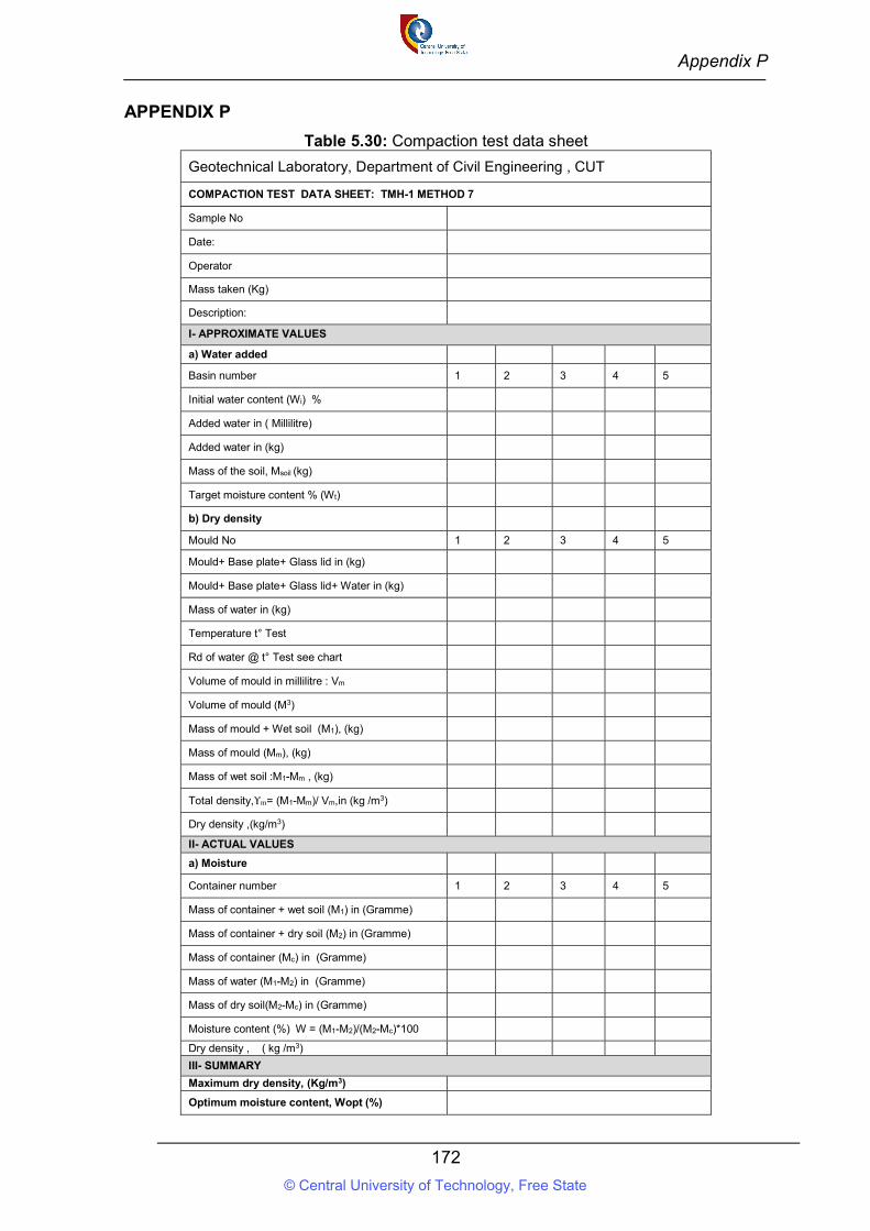
Appendix P

172

APPENDIX P

Table 5.30: Compaction test data sheet

Geotechnical Laboratory, Department of Civil Engineering , CUT

COMPACTION TEST DATA SHEET: TMH-1 METHOD 7

Sample No

Date:

Operator

Mass taken (Kg)

Description:

I- APPROXIMATE VALUES

a) Water added

Basin number 1 2 3 4 5

Initial water content (Wi) %

Added water in ( Millilitre)

Added water in (kg)

Mass of the soil, Msoil (kg)

Target moisture content % (Wt)

b) Dry density

Mould No 1 2 3 4 5

Mould+ Base plate+ Glass lid in (kg)

Mould+ Base plate+ Glass lid+ Water in (kg)

Mass of water in (kg)

Temperature t° Test

Rd of water @ t° Test see chart

Volume of mould in millilitre : Vm

Volume of mould (M3)

Mass of mould + Wet soil (M1), (kg)

Mass of mould (Mm), (kg)

Mass of wet soil :M1-Mm , (kg)

Total density,Υm= (M1-Mm)/ Vm,in (kg /m3)

Dry density ,(kg/m3)

II- ACTUAL VALUES

a) Moisture

Container number 1 2 3 4 5

Mass of container + wet soil (M1) in (Gramme)

Mass of container + dry soil (M2) in (Gramme)

Mass of container (Mc) in (Gramme)

Mass of water (M1-M2) in (Gramme)

Mass of dry soil(M2-Mc) in (Gramme)

Moisture content (%) W = (M1-M2)/(M2-Mc)*100

Dry density , ( kg /m3)

III- SUMMARY

Maximum dry density, (Kg/m3)

Optimum moisture content, Wopt (%)


Appendix Q

173

APPENDIX Q

Table 5.31: Measurement of soil suction using filter paper- Data sheet ASTM D 5298 (1994) Geotechnical Laboratory, Department of Civil Engineering , CUT

Soil designation …………………

Date tested: ………………….

Tested by: ………………….. Sample 1-1 1-2 1-3 1-4 1-5

Gravimetric water content of soil sample,W, ( %)

Tin No

Top filter paper / Bottom filter paper Top Bot Top Bot Top Bot Top Bot Top Bot

Cold Tare Mass, g Tc

Mass of wet Filter paper + Cold Tare Mass, g m1

Mass of Dry Filter paper + Hot Tare Mass, g m2

Hot Tare Mass, g Th

Mass of water in Filter Paper, g M2-Th Mf

Mass of water in Filter Paper, g M1-M2-Tc+Th Mw

Water content of filter Paper,g (Mw/Mf) % Wf

Suction , kPa Ψ

Suction , logkPa Ψ

Suction, PF = logkPa+1 Ψ


174


CHARACTERIZATION OF SWELLING STRESS AND SOIL ...

Documents