Characterization of spinal cord compression

DISSERTATION

submitted to

Aix-Marseille University

Doctoral School of Life and Health Sciences

for the degree of

Doctor of Philosophy (Ph.D.)

Characterization of spinal cord compression:

Development of 7 Tesla Magnetic Resonance

techniques for human spinal cord perfusion imaging

and biomechanical simulation of Degenerative

Cervical Myelopathy

put forward by

Simon LÉVY, Eng., M.A.Sc.

Oral examination: September 24, 2020


Characterization of spinal cord compression:

Development of 7 Tesla Magnetic Resonance techniques for human spinal cord perfusion imaging and

biomechanical simulation of Degenerative Cervical Myelopathy

DISSERTATION, September 24, 2020

Reviewers: Dr. Alexandre VIGNAUD and Pr. Éric WAGNAC

Examiners: Dr. Alan SIEFERT, Dr. Thomas TROALEN and Pr. Pierre-Hugues ROCHE

Supervisors: Dr. Virginie CALLOT and Dr. Pierre-Jean ARNOUX

Aix-Marseille University

Center for Magnetic Resonance in Biology and Medicine (CRMBM)

Laboratory of Applied Biomechanics (LBA)

Faculty of Medicine

Doctoral School of Life and Health Sciences

27 Boulevard Jean Moulin

13385 Marseille

UNIVERSITÉ D’AIX-MARSEILLE

ÉCOLE DOCTORALE Sciences de la Vie et de la Santé

Partenaires de recherche

Siemens Healthineers & Assistance Publique Hôpitaux de Marseille

Laboratoires

Centre de Résonance Magnétique en Biologie et Médecine (CRMBM)

Unité Mixte de Recherche 7339 CNRS/AMU

Laboratoire de Biomécanique Appliquée (LBA)

Unité Mixte de Recherche T24 AMU/Université Gustave Eiffel

International Laboratory for Imaging and Biomechanics of the Spine (iLab-Spine)

Thèse présentée pour obtenir le grade universitaire de docteur

Discipline : Neurosciences


Caractérisation des compressions médullaires :

Développement de techniques d’Imagerie par Résonance Magnétique de

perfusion de la moelle épinière humaine à 7 Tesla et simulation

biomécanique des Myélopathies Cervicales Dégénératives

Characterization of spinal cord compressions:

Development of 7 Tesla Magnetic Resonance techniques for human spinal cord

perfusion imaging and biomechanical simulation of Degenerative Cervical Myelopathy

Soutenue le 24/09/2020 devant le jury composé de :

Alexandre VIGNAUD, HDR. Neurospin, CEA, Saclay, France Rapporteur

Éric WAGNAC, Pr. École de Technologie Supérieure, Montréal, Canada Rapporteur

Alan SEIFERT, PhD. Icahn School of Medicine, New York, USA Examinateur

Thomas TROALEN, PhD. Siemens Healthineers, Saint-Denis, France Examinateur

Pierre-Hugues ROCHE, MD.,Pr. Hopital Nord, APHM, Marseille, France Examinateur

Virginie CALLOT, HDR. CRMBM, CNRS/AMU, Marseille, France Directrice de thèse

Pierre-Jean ARNOUX, HDR. LBA, Univ Gustave Eiffel/AMU, Marseille, France Co-directeur de thèse

Numéro national de thèse/suffixe local : 2017AIXM0001/001ED62

To my grand-parents,

Lucie, Nicole, Emile and Georges,

Résumé

Les compressions médullaires induites par la dégénérescence du rachis sont une cause

fréquente de dysfonctionnement de la moelle épinière. Des recherches antérieures ont

démontré des signes d’ischémie déclenchant l’apoptose des cellules, exacerbés par la

suite par un processus d’inflammation, menant finalement à la myélopathie et l’altération

fonctionnelle. Cependant, la durée des processus dégénératifs et leur interaction restent

peu connues. Si la chirurgie de décompression est recommandée pour les Myélopathies

Cervicales Dégénératives (DCM) sévères, le suivi et la prise en charge des cas légers

sont plus problématiques. Un biomarqueur du déficit de perfusion serait d’une aide

particulièrement précieuse dans la prise de décision.

Ce travail de thèse s’inscrit dans un projet plus global visant à combiner la simulation

biomécanique des contraintes induites avec des mesures de perfusion in-vivo par IRM.

Plus particulièrement, ce travail visait à développer une technique IRM de cartographie

de la perfusion médullaire et à concevoir des simulations par éléments finis réalistes de

cas de compressions DCM typiques.

Compte tenu des faibles niveaux de perfusion et de la petite taille de la moelle épinière

humaine, les développements ont été réalisés à 7T pour bénéficier de la sensibilité accrue

à ultra-haut champ. La technique de Mouvement Incohérent Intra-Voxel (IVIM) a tout

d’abord été étudiée. Le rapport signal/bruit a été maximisé et les erreurs obtenues in-vivo

ont été évaluées à l’aide de simulations de Monte-Carlo. L’imagerie par Contraste de

Susceptibilité Dynamique (DSC), basée sur l’injection d’un agent de contraste, a ensuite

été explorée. Un protocole d’acquisition et de post-traitement a été mis en place pour

minimiser les biais physiologiques (battements cardiaques, respiration, mouvement).

Enfin, des caractéristiques géométriques typiques des compressions DCM ont été extraites

de la littérature et d’IRM anatomiques de patients. Des simulations biomécaniques ont

été implémentées à l’aide d’un modèle détaillé du rachis et les contraintes résultantes ont

été quantifiées au long du processus de compression, le long de la moelle ainsi que par

région médullaire.

La technique IVIM a démontré une faible sensibilité malgré le rapport signal/bruit

élevé obtenu. En revanche, des cartes bien définies de volume et flux sanguin relatifs

ont été obtenues chez des volontaires sains par DCM, mettant en évidence la perfusion

plus élevée de la substance grise par rapport à la substance blanche. La sensibilité a

été plus limitée chez les patients DCM, mais de nouvelles consignes pour améliorer

la robustesse de la technique ont pu être identifiées. Les simulations biomécaniques

pourraient expliquer l’ischémie fréquemment observée chez les patients DCM dans la

substance grise, mais elles ne peuvent expliquer directement la démyélinisation de la

voie corticospinale si l’on se base sur la distribution des contraintes uniquement.

En conclusion, la technique DSC a un grand potentiel pour la cartographie de la

perfusion de la moelle épinière humaine en routine clinique. Étant donné la grande

variabilité des motifs de compression DCM et des symptômes qui en résultent, la définition

de simulations standards est complexe. Dans ce contexte, une approche spécifique au

patient est recommandée pour pouvoir établir de manière fiable une relation entre la

compression mécanique et l’ischémie induite.vii

Abstract

Spinal cord compression induced by spine degeneration is a common cause of spinal

cord dysfunction. Previous research has shown evidence of ischemia firing cell apoptosis

exacerbated by inflammation, which eventually results in myelopathy and functional

impairment. However, little is known about the timescale of the processes and their

interaction. If decompression surgery is recommended for severe Degenerative Cervical

Myelopathy (DCM), the progression and management of mild cases is more challenging.

Biomarker of perfusion deficit would particularly help to make decision.

This PhD is part of a global project aiming at associating biomechanical simulations of

the induced constraints to in-vivo measurements of perfusion using MRI. More specifically,

this work aimed at developing an MRI technique to map spinal cord perfusion and at

designing realistic finite element simulations of typical DCM compressions.

Given the low perfusion levels and small size of the human spinal cord, developments

were conducted at 7T to benefit from ultra-high field sensitivity. The Intra-Voxel Incoherent

Motion (IVIM) technique was first investigated. Signal-to-noise ratio was maximized

and errors from in-vivo data were assessed using Monte-Carlo simulations. Dynamic

Susceptibility Contrast (DSC) imaging, which makes use of contrast injection, was then

explored. Acquisition and post-processing pipelines were implemented to address phys-

iological biases (heartbeat, breathing, motion). Finally, geometrical features of typical

DCM compressions were synthesized from literature and anatomical MRI of patients.

Simulations were performed using a detailed spine model and resulting constraints were

quantified along the compression process, spinal cord length and across spinal pathways.

The IVIM technique showed poor sensitivity despite the high signal-to-noise ratio

obtained. By contrast, well-defined relative blood volume and flow maps were obtained

in healthy volunteers with DSC, depicting the higher perfusion of gray matter with respect

to white matter. Sensitivity was mitigated in DCM patients, however new guidelines to

improve robustness of the technique could be identified. Based on stress distribution

only, biomechanical simulations could explain the gray matter infarction reported in DCM

patients but not directly the demyelination of the corticospinal tract.

In conclusion, the DSC technique has a great potential for human spinal cord per-

fusion mapping in clinical routine. Given the large variability of DCM patterns and

resulting symptoms, the definition of standard simulation designs is complex. In this con-

text, a patient-specific approach is advised to reliably establish the relationship between

mechanical compression and resulting ischemia.

ix

Acknowledgement

First of all, I want to thank all the people who worked so that the DOC2AMU doctoral

program takes shape and offers a fruitful and enlightening PhD environment. In particular,

I would like to thank Pr. Mossadek Talby and Sarah Sawyer for coordinating the program

and for their goodwill along those three years, as well as A*MIDEX and the Regional

Council Provence-Alpes-Côte d’Azur for funding the program along with Aix-Marseille

University.

Obviously, I want to thank Virginie Callot and Pierre-Jean Arnoux for setting up this

exciting project and trusting me for carrying it out. Thank you for your commitment and

positiveness, and for the skills I have learned along those three years. I also want to truly

thank Stanislas Rapacchi from who I learned so much. Thank you for your support, your

enthusiasm, your generosity and above all, your precious help. We both know that I owe

you much more than this.

I am also extremely grateful to Thomas Troalen for his tutorship and valuable help.

Along with Siemens Healthineers, I would like to thank Thorsten Feiweier for the support.

I am sincerely grateful to Tangi Roussel, Olivier Girard, Ludovic De Rochefort and Arnaud

Le Troter for the stimulating discussions and for everything they helped me figure out.

Thank you for your openness. Many thanks also to Christophe Vilmen for his amazing

help on the conception of the phantom. And thank you very much to Laure Balasse for

welcoming us at the CERIMED and for your time.

Furthermore, I am sincerely grateful to Sylviane Confort-Gouny, Véronique Gimenez-

Derderian, Lauriane Pini and Patrick Viout for their devotion to the lab and its activity,

and for their previous help all along those three years. Thank you also to Monique

Bernard and Maxime Guye for sympathetically welcoming me in this lab and supporting

my initiatives and projects. Thank you to Jean-Philippe Ranjeva for taking care of the

exchange within the group with zeal. I am extremely grateful to Magatte Sarr and

Danielle Rousseau for all the administrative burden that my missions outside the lab

generated. Thank you very much also to all the students of the lab for constantly working

for a warmer and more cohesive group. In particular, I would like to thank Emyra Trabelsi

for her limitless kindhearted and generous support. And many thanks to all the people of

the lab I could not name here!

xi

From the side of the LBA, I would like to particularly thank Patrice Sudres, Tristan

Tarrade, Maxime Llari and Morgane Evin for their help and useful discussions. I am also

extremely grateful to all the students for the warm and stimulating atmosphere they

constantly fuel in the lab. Many thanks also to Pierre-Hugues Roche for your time, your

support and your heated interest for the project.

From abroad, I would like to truly thank Maryam Seif, Patrick Freund and Johanna

Vannesjö for their hearty welcome in Zurich and their interest in my work. I am also

extremely grateful to Alan Seifert for his commitment and support to make my research

exchange in New York come true despite the circumstances. And I would like to express

my sincere appreciation and thanks to Laura Bell and Steven Sourbron for all the energy

and devotion you have dedicated, and continue to dedicate, to OSIPI.

Finally, I would like to thank all the DOC2AMU fellows who became my second family

during those three years in Marseille. And I will end by thanking the most essential

support: my family, including Michaela. I am endlessly grateful for your sound advice,

ardent encouragement and constant presence despite the distance.

xii

Contents

1 Introduction 5

1.1 Motivation . . . . . . . . . . . . . . . . . . . . . . . . . . . . . . . . . . . . 5

1.2 Scope . . . . . . . . . . . . . . . . . . . . . . . . . . . . . . . . . . . . . . 8

2 General Background 11

2.1 The human spinal cord . . . . . . . . . . . . . . . . . . . . . . . . . . . . . 11

2.1.1 Structure . . . . . . . . . . . . . . . . . . . . . . . . . . . . . . . . 11

2.1.2 Gray matter . . . . . . . . . . . . . . . . . . . . . . . . . . . . . . . 13

2.1.3 White matter . . . . . . . . . . . . . . . . . . . . . . . . . . . . . . 14

2.1.4 Vascular network . . . . . . . . . . . . . . . . . . . . . . . . . . . . 15

2.2 Magnetic Resonance Imaging acquisition . . . . . . . . . . . . . . . . . . . 19

2.2.1 Nuclear Magnetic Resonance signal . . . . . . . . . . . . . . . . . . 20

2.2.2 Image acquisition and reconstruction . . . . . . . . . . . . . . . . . 28

2.3 Ultrahigh field MRI . . . . . . . . . . . . . . . . . . . . . . . . . . . . . . . 37

2.3.1 Advantages of UHF MRI . . . . . . . . . . . . . . . . . . . . . . . . 39

2.3.2 Disadvantages and challenges of UHF MRI . . . . . . . . . . . . . . 44

2.3.3 UHF MRI in spinal cord . . . . . . . . . . . . . . . . . . . . . . . . 50

2.4 Perfusion MRI . . . . . . . . . . . . . . . . . . . . . . . . . . . . . . . . . . 56

2.4.1 Exogenous techniques . . . . . . . . . . . . . . . . . . . . . . . . . 56

2.4.2 Vascular Occupancy (VASO) MRI . . . . . . . . . . . . . . . . . . . 68

2.4.3 Endogenous techniques . . . . . . . . . . . . . . . . . . . . . . . . 68

2.4.4 State of the art in spinal cord . . . . . . . . . . . . . . . . . . . . . 79

2.5 Degenerative Cervical Myelopathy . . . . . . . . . . . . . . . . . . . . . . 85

2.5.1 Pathogenesis . . . . . . . . . . . . . . . . . . . . . . . . . . . . . . 85

2.5.2 Diagnosis . . . . . . . . . . . . . . . . . . . . . . . . . . . . . . . . 91

2.5.3 Treatment . . . . . . . . . . . . . . . . . . . . . . . . . . . . . . . . 94

2.5.4 Epidemiology . . . . . . . . . . . . . . . . . . . . . . . . . . . . . . 94

2.5.5 Application of electrophysiology in DCM . . . . . . . . . . . . . . . 96

xiii

2.5.6 Application of multi-parametric quantitative MRI in DCM . . . . . 97

2.6 Biomechanical modeling of spinal cord compression . . . . . . . . . . . . . 98

2.6.1 Finite element modeling . . . . . . . . . . . . . . . . . . . . . . . . 99

2.6.2 Finite element modeling of spinal cord compressions . . . . . . . . 103

2.6.3 The Spine Model for Safety and Surgery (SM2S) . . . . . . . . . . 113

3 Thesis objectives and structure 117

3.1 Research questions . . . . . . . . . . . . . . . . . . . . . . . . . . . . . . . 117

3.2 Objectives . . . . . . . . . . . . . . . . . . . . . . . . . . . . . . . . . . . . 118

4 Intra-Voxel Incoherent Motion at 7 Tesla to quantify human spinal cord

perfusion: limitations and promises 121

4.1 Foreword . . . . . . . . . . . . . . . . . . . . . . . . . . . . . . . . . . . . 121

4.2 Manuscript . . . . . . . . . . . . . . . . . . . . . . . . . . . . . . . . . . . 121

4.3 Concluding remarks . . . . . . . . . . . . . . . . . . . . . . . . . . . . . . 142

5 Feasibility of human spinal cord perfusion mapping using Dynamic Suscep-

tibility Contrast imaging at 7T: preliminary results and identified guidelines143

5.1 Foreword . . . . . . . . . . . . . . . . . . . . . . . . . . . . . . . . . . . . 143

5.2 Manuscript . . . . . . . . . . . . . . . . . . . . . . . . . . . . . . . . . . . 144


6 Biomechanical comparison of spinal cord compression types occurring in

Degenerative Cervical Myelopathy 169

6.1 Foreword . . . . . . . . . . . . . . . . . . . . . . . . . . . . . . . . . . . . 169

6.2 Manuscript . . . . . . . . . . . . . . . . . . . . . . . . . . . . . . . . . . . 170


7 General discussion 195

7.1 Assessing perfusion status of the human spinal cord . . . . . . . . . . . . . 195

7.1.1 Achievements . . . . . . . . . . . . . . . . . . . . . . . . . . . . . . 195

7.1.2 Major hurdles . . . . . . . . . . . . . . . . . . . . . . . . . . . . . . 199

7.1.3 Optimizations to focus on . . . . . . . . . . . . . . . . . . . . . . . 201

7.1.4 Benefits and drawbacks of Ultra-High Field . . . . . . . . . . . . . 203

7.1.5 Perspectives . . . . . . . . . . . . . . . . . . . . . . . . . . . . . . . 207

7.2 Biomechanical modeling of DCM-like spinal cord compression . . . . . . . 212

7.2.1 Achievements . . . . . . . . . . . . . . . . . . . . . . . . . . . . . . 212

7.2.2 Model validity . . . . . . . . . . . . . . . . . . . . . . . . . . . . . . 214

xiv

7.2.3 Perspectives . . . . . . . . . . . . . . . . . . . . . . . . . . . . . . . 216

7.3 Relating perfusion and mechanical constraints in chronic spinal cord com-

pression . . . . . . . . . . . . . . . . . . . . . . . . . . . . . . . . . . . . . 217

8 General conclusion 221

9 Publications, communications and international commitments 225

A Appendix 233

A.1 Magnetic Resonance Angiography (MRA) . . . . . . . . . . . . . . . . . . 233

A.1.1 Digital Subtraction Angiography . . . . . . . . . . . . . . . . . . . 233

A.1.2 Non-contrast MRA . . . . . . . . . . . . . . . . . . . . . . . . . . . 233

A.1.3 Contrast-enhanced MRA . . . . . . . . . . . . . . . . . . . . . . . . 234

A.2 Vascular Occupancy (VASO) MRI . . . . . . . . . . . . . . . . . . . . . . . 236

A.3 Grading tools to quantify patients’ neurological status in Degenerative

Cervical Myelopathy . . . . . . . . . . . . . . . . . . . . . . . . . . . . . . 239

A.3.1 Nurick’s grading system (Nurick, 1972) . . . . . . . . . . . . . . . 239

A.3.2 Modified Japanese Orthopedic Association Scale (mJOA) . . . . . . 240

A.4 Conception of a perfusion phantom . . . . . . . . . . . . . . . . . . . . . . 241

Bibliography 247

xv

List of Figures

2.1 Spinal cord structure . . . . . . . . . . . . . . . . . . . . . . . . . . . . . . . 12

2.2 Spinal cord CSA evolution along inferior-superior axis . . . . . . . . . . . . 13

2.3 Main cell groups in spinal gray matter . . . . . . . . . . . . . . . . . . . . . 14

2.4 Major spinal pathways . . . . . . . . . . . . . . . . . . . . . . . . . . . . . . 15

2.5 Spinal arterial supply . . . . . . . . . . . . . . . . . . . . . . . . . . . . . . . 16

2.6 Transversal view of spinal cord vascular network . . . . . . . . . . . . . . . 17

2.7 Spinal venous drainage . . . . . . . . . . . . . . . . . . . . . . . . . . . . . . 19

2.8 Spin precession . . . . . . . . . . . . . . . . . . . . . . . . . . . . . . . . . . 20

2.9 Nuclear magnetic resonance experience . . . . . . . . . . . . . . . . . . . . 23

2.10 NMR signal acquisition . . . . . . . . . . . . . . . . . . . . . . . . . . . . . . 25

2.11 Gradient-echo and spin-echo sequences diagrams for illustration purposes . 27

2.12 Relation between k-space and image space sampling parameters in two

dimensions . . . . . . . . . . . . . . . . . . . . . . . . . . . . . . . . . . . . 30

2.13 Relation between position and frequency with application of a slice-selection

gradient . . . . . . . . . . . . . . . . . . . . . . . . . . . . . . . . . . . . . . 31

2.14 Example of k-space trajectory with associated pulse sequence diagram . . . 32

2.15 GRAPPA: estimation of the missing points . . . . . . . . . . . . . . . . . . . 34

2.16 Sequence diagram and k-space trajectory for circular spiral EPI . . . . . . . 35

2.17 Differences in the type of artifacts obtained in spinal cord with a Gradient-

echo (GRE) sequence and spiral EPI or standard EPI readouts . . . . . . . . 37

2.18 Ultimate intrinsic SNR (uiSNR or uSNR) increase with field strength as a

function of the position in human head model . . . . . . . . . . . . . . . . . 41

2.19 In-vivo measured SNR and g-factor in brain as a function of field strength . 41

2.20 Proportion of tumbling molecules according to the frequency and effect of

field strength increase . . . . . . . . . . . . . . . . . . . . . . . . . . . . . . 42

2.21 R∗

2 in brain gray and white matter (averaged over 6 healthy subjects) as a

function of field strength . . . . . . . . . . . . . . . . . . . . . . . . . . . . . 43

xvii

2.22 Measured B0 difference in the spinal cord between expired and inspired

breath-hold field map acquisitions according to the vertebral level at 3T and

7T . . . . . . . . . . . . . . . . . . . . . . . . . . . . . . . . . . . . . . . . . 46

2.23 Cervical spine coil array for 7T MRI designed by RAPID Biomedical . . . . . 51

2.24 Two-panel coil array proposed by Zhang et al. (2017) for 7 T MRI of the

brainstem and cervical spinal cord . . . . . . . . . . . . . . . . . . . . . . . 52

2.25 Integrated AC/DC 15-channel Rx and 3-dipole Tx array design for 7T MRI

of cervical spine . . . . . . . . . . . . . . . . . . . . . . . . . . . . . . . . . . 53

2.26 Reproducibility of resting state function MRI in spinal cord at 7T . . . . . . 54

2.27 Examples of applications benefiting from 7T MRI . . . . . . . . . . . . . . . 55

2.28 Relaxation rate R1 of Dotarem® in human blood at 37°C according to Gd

concentration and field strength . . . . . . . . . . . . . . . . . . . . . . . . . 57

2.29 Contrast agent r1 dependency on field strength in human blood at 37°C for

different chelates . . . . . . . . . . . . . . . . . . . . . . . . . . . . . . . . . 58

2.30 T2 relaxivities in distilled water and human plasma at 1.5T, 3T and 7T and

in human blood at 1.5T and 3T . . . . . . . . . . . . . . . . . . . . . . . . . 59

2.31 R∗

2 of Magnevist™(Gd-DTPA) in bovine blood and oxygenated human blood

at 37°C according to Kalavagunta et al. (2010) and Kalavagunta et al. (2014) 60

2.32 CA bolus effect on MRI signal intensity in DSC imaging, along with effect of

CA leakage in extravascular space . . . . . . . . . . . . . . . . . . . . . . . . 60

2.33 Relative perfusion indices and summary parameters defined on concentration

(in mM) time curve . . . . . . . . . . . . . . . . . . . . . . . . . . . . . . . . 63

2.34 Relative cerebral BF maps from GRE and SE . . . . . . . . . . . . . . . . . . 65

2.35 ∆R2 and ∆R∗

2 dependency on vessel diameter . . . . . . . . . . . . . . . . . 66

2.36 Example of 2-compartment pharmacokinetic models of DCE and derived

perfusion parameters . . . . . . . . . . . . . . . . . . . . . . . . . . . . . . . 67

2.37 Comparison of BV and BF maps obtained from typical DSC (T2*-weighted

images) and DCE (T1-weighted images) protocolsDCE . . . . . . . . . . . . 69

2.38 Different ASL labeling approaches . . . . . . . . . . . . . . . . . . . . . . . . 70

2.39 Comparison of perfusion parameter maps obtained from PASL and DSC MRI

in acute ischemic stroke . . . . . . . . . . . . . . . . . . . . . . . . . . . . . 72

2.40 DWI: sensitization of MRI signal to water diffusion . . . . . . . . . . . . . . 74

2.41 Calculation of the diffusion tensor . . . . . . . . . . . . . . . . . . . . . . . . 75

2.42 Intra-Voxel Incoherent Motion (IVIM) model and signal representation . . . 77

2.43 Brain and spinal cord BF maps measured in the mouse using ASL . . . . . . 80

xviii

2.44 BF maps obtained in the human spinal cord with ASL at 3T (Nair et al.,

2010) and 1.5T (Girard et al., 2013) . . . . . . . . . . . . . . . . . . . . . . 81

2.45 Spinal cord BV map (e) derived from acquisitions pre- (a, c) and post-contrast

(b,d) agent injection within one subject and one slice obtained with VASO

MRI by Lu et al. (2008) . . . . . . . . . . . . . . . . . . . . . . . . . . . . . 82

2.46 Identification of the Anterior Spinal Artery and artery of Adamkiewicz using

Digital Subtraction Angiography . . . . . . . . . . . . . . . . . . . . . . . . . 83

2.47 Identification of the Anterior Spinal Artery in cervical region using contrast-

enhanced Magnetic Resonance Angiography . . . . . . . . . . . . . . . . . . 84

2.48 Conceptual classification of the pathological processes encountered in De-

generative Cervical Myelopathy (DCM) by Nouri et al. (2015) . . . . . . . . 86

2.49 Illustration of the different anatomical degenerations found in Degenerative

Cervical Myelopathy . . . . . . . . . . . . . . . . . . . . . . . . . . . . . . . 87

2.50 Pathobiological effects of static and chronic cervical cord compression ac-

cording to Kalsi-Ryan et al. (2012) . . . . . . . . . . . . . . . . . . . . . . . 88

2.51 Example of clinical grading scale for spinal canal stenosis . . . . . . . . . . . 93

2.52 Classical definition of 3D stresses on a cube . . . . . . . . . . . . . . . . . . 102

2.53 Typical stress-strain curve derived from measurement during a tensile exper-

iment . . . . . . . . . . . . . . . . . . . . . . . . . . . . . . . . . . . . . . . 103

2.54 Strain-stress curves measured in the main studies for spinal cord under

tensile loading . . . . . . . . . . . . . . . . . . . . . . . . . . . . . . . . . . 104

2.55 Intervertebral disc anatomy . . . . . . . . . . . . . . . . . . . . . . . . . . . 107

2.56 Multi-level compression designs with different transverse profiles for simula-

tions of ossification of the posterior longitudinal ligament by Khuyagbaatar

et al. (2015) . . . . . . . . . . . . . . . . . . . . . . . . . . . . . . . . . . . . 112

2.57 Finite element model of the spinal cord including anterior spinal arteries

and five branches from Alshareef et al. (2014) . . . . . . . . . . . . . . . . . 113

2.58 Progressive developments of the Spine Model for Safety and Surgery (SM2S)116

3.1 Thesis general structure . . . . . . . . . . . . . . . . . . . . . . . . . . . . . 119

5.1 Acquisition characteristics . . . . . . . . . . . . . . . . . . . . . . . . . . . . 148

5.2 Signal processing pipeline . . . . . . . . . . . . . . . . . . . . . . . . . . . . 151

5.3 Image quality, frequent artifacts and effects of GRAPPA calibration and EPI

phase correction in spin-echo and gradient-echo high-resolution EPI . . . . . 152

5.4 Breathing-induced signal fluctuations in spin-echo and gradient-echo high-

resolution single-shot EPI . . . . . . . . . . . . . . . . . . . . . . . . . . . . 154

xix

5.5 DSC results in 3 healthy volunteers at 7T . . . . . . . . . . . . . . . . . . . . 156

5.6 DSC results in 5 patients at 7T . . . . . . . . . . . . . . . . . . . . . . . . . . 157

5.7 Examples of perfusion index maps that can be obtained from DSC in spinal

cord at 7T . . . . . . . . . . . . . . . . . . . . . . . . . . . . . . . . . . . . . 158

6.1 Definition of the compression indices measured on anatomical MRI data. . . 175

6.2 Main compression types observed in the DCM group . . . . . . . . . . . . . 178

6.3 Constraints value along the inferior-superior axis for each compression type 182

6.4 Constraints value along the development of the compression until threshold 183

6.5 Spinal cord regions analysis at compression threshold . . . . . . . . . . . . . 184

7.1 Temporal SNR as a function of the SNR of a single time repetition (thermal

noise) . . . . . . . . . . . . . . . . . . . . . . . . . . . . . . . . . . . . . . . 201

7.2 Comparison between IVIM and ASL in the monitoring of perfusion changes

in the injured mice . . . . . . . . . . . . . . . . . . . . . . . . . . . . . . . . 211

7.3 Signal in cord from control and tag images using PCASL at 1.5T . . . . . . . 211

9.1 Logo and current governance structure of OSIPI . . . . . . . . . . . . . . . . 230

A.1 Principle of Time-Of-Flight (TOF) MRA using gradient-echo or spin-echo

sequence . . . . . . . . . . . . . . . . . . . . . . . . . . . . . . . . . . . . . . 235

A.2 Phase-contrast technique . . . . . . . . . . . . . . . . . . . . . . . . . . . . . 236

A.3 Principle of the VASO MRI technique first applied to remove contribution of

blood vessels to BOLD signal in functional MRI . . . . . . . . . . . . . . . . 237

A.4 In-house perfusion phantom . . . . . . . . . . . . . . . . . . . . . . . . . . . 244

A.5 Comparison between IVIM and ASL in the monitoring of perfusion changes

in the injured mice . . . . . . . . . . . . . . . . . . . . . . . . . . . . . . . . 245

xx

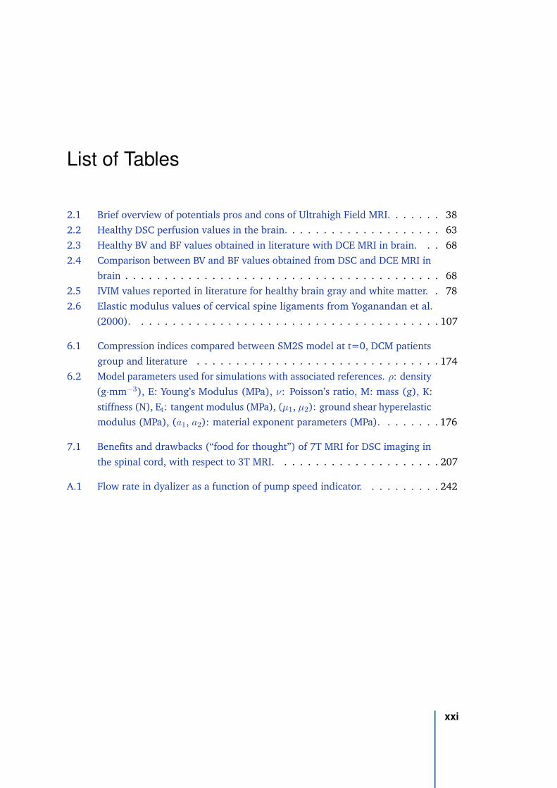
List of Tables

2.1 Brief overview of potentials pros and cons of Ultrahigh Field MRI. . . . . . . 38

2.2 Healthy DSC perfusion values in the brain. . . . . . . . . . . . . . . . . . . . 63

2.3 Healthy BV and BF values obtained in literature with DCE MRI in brain. . . 68

2.4 Comparison between BV and BF values obtained from DSC and DCE MRI in

brain . . . . . . . . . . . . . . . . . . . . . . . . . . . . . . . . . . . . . . . . 68

2.5 IVIM values reported in literature for healthy brain gray and white matter. . 78

2.6 Elastic modulus values of cervical spine ligaments from Yoganandan et al.

(2000). . . . . . . . . . . . . . . . . . . . . . . . . . . . . . . . . . . . . . . 107

6.1 Compression indices compared between SM2S model at t=0, DCM patients

group and literature . . . . . . . . . . . . . . . . . . . . . . . . . . . . . . . 174

6.2 Model parameters used for simulations with associated references. ρ: density

(g·mm−3), E: Young’s Modulus (MPa), ν: Poisson’s ratio, M: mass (g), K:

stiffness (N), Et: tangent modulus (MPa), (µ1, µ2): ground shear hyperelastic

modulus (MPa), (a1, a2): material exponent parameters (MPa). . . . . . . . 176

7.1 Benefits and drawbacks (“food for thought”) of 7T MRI for DSC imaging in

the spinal cord, with respect to 3T MRI. . . . . . . . . . . . . . . . . . . . . 207

A.1 Flow rate in dyalizer as a function of pump speed indicator. . . . . . . . . . 242

xxi

Acronyms

ADC Analog/Digital Converter. 30, 32

AIF Arterial Input Function. 61, 66, 198, 199, 210, 221, 239

ASA Anterior Spinal Artery. xix, 16, 17, 18, 83, 84, 112, 199, 210, 221

ASL Arterial Spin Labeling. xviii, 7, 38, 42, 69, 70, 73, 78, 80, 108, 120, 195, 196, 199,

210, 211

ATT Arterial Transit Time. 71, 72

BAT Bolus Arrival Time. 61, 62

BF Blood Flow. xviii, xxi, 62, 63, 67, 68, 69, 70, 71, 72, 79, 80, 167, 209, 222, 239

BOLD Blood Oxygen Level Dependent. xx, 38, 43, 236, 237

BV Blood Volume. xviii, xxi, 62, 63, 67, 68, 69, 81, 167, 209, 222, 237, 238, 239

BW bandwidth. 31, 45

CA Contrast agent. 56, 57, 73, 195, 233, 235

CASL Continuous ASL. 70, 71

CNR Contrast-to-Noise Ratio. 38, 64, 239

CSA Cross-Sectional Area. 97, 105, 111, 169, 212, 222

CSF Cerebrospinal fluid. 11, 12, 13, 14, 45, 75, 79, 80, 111, 112, 114, 196, 198, 199,

200, 205, 238

DCE Dynamic Contrast-Enhanced. xviii, xxi, 38, 66, 67, 68, 69, 81, 195, 196, 202, 209,

210, 234

1

DCM Degenerative Cervical Myelopathy. xix, 6, 9, 85, 86, 87, 94, 96, 97, 98, 101, 109,

113, 115, 117, 118, 143, 169, 170, 171, 193, 195, 197, 206, 209, 212, 213, 216,

218, 221, 222

DSA Digital Subtraction Angiography. xix, 83, 196, 233, 234

DSC Dynamic Susceptibility Contrast. xviii, xxi, 38, 43, 59, 60, 66, 67, 68, 72, 78, 81,

119, 120, 143, 167, 195, 196, 197, 198, 202, 206, 209, 222, 239

DTI Diffusion Tensor Imaging. 38, 52, 75, 76, 97, 196, 209

DWI Diffusion-Weighted Imaging. xviii, 38, 73, 74, 76

EPI Echo-Planar Imaging. 32, 33, 36, 44, 45, 47, 64, 81, 143, 198, 200, 202, 203, 206,

209, 239

FA Fractional Anisotropy. 55, 75

FID Free-Induction Decay. 25, 47

FOV Field-Of-View. 30, 47

Gd Gadolinium. 56, 57, 68, 69

GM Gray Matter. 63, 67, 68, 77, 78, 79, 87, 97, 105, 111, 211, 238

GRAPPA GeneRalized Autocalibrating Partially Parallel Acquisitions. xvii, 33, 34, 35,

206

GRE Gradient-echo. xvii, 26, 36, 37, 38, 52, 59, 198, 203, 206, 209, 234

ISMRM International Society for Magnetic Resonance in Medicine. 121, 143, 226, 227,

228, 229, 231

IVIM Intra-Voxel Incoherent Motion. xviii, xxi, 76, 77, 78, 79, 80, 119, 120, 121, 142,

143, 167, 195, 196, 198, 199, 200, 202, 221, 242

MD Mean Diffusivity. 75

MEP Motor Evoked Potential. 96, 97

mJOA modified Japanese Orthopaedic Association. 81

2 Acronyms

MRA Magnetic Resonance Angiography. xix, xx, 56, 82, 84, 210, 212, 217, 233, 234,

235, 236

MRE Magnetic Resonance Elastography. 108, 219

MRI Magnetic Resonance Imaging. 6, 7, 8, 20, 118, 121, 199

MRS Magnetic Resonance Spectroscopy. 44, 52, 97

MTT Mean Transit Time. 62, 63, 67, 239

NMR Nuclear Magnetic Resonance. 19, 20, 22, 24, 39

OPLL Ossification of the Posterior Longitudinal Ligament. 6, 85, 87, 96, 110, 111

PASL Pulsed ASL. 70, 71, 79, 80, 81, 210

PCASL Pseudo-Continuous ASL. 70, 71, 72, 79, 211

PLD Post-Label Delay. 69, 70, 71, 80

PSA Posterior Spinal Arteries. 17, 18, 83, 199, 210, 221

PVE Partial Volume Effects. 61

rBF relative Blood Flow. 62

rBV relative Blood Volume. 62, 81

RD Radial Diffusivity. 75

RF Radio-frequency. 23, 26, 38, 39, 69, 73, 142, 234, 236

ROI Region-Of-Interest. 79, 82, 204, 213, 218

Rx Receive. 51

SAR Specific Absorption Rate. 48, 73, 167, 198, 202, 203

SD Standard-Deviation. 77

SE Spin-echo. 26, 36, 38, 59, 234

SEP Somatosensory Evoked Potential. 96, 97

Acronyms 3

SM2S Spine Model for Safety and Surgery. xix, 113, 114, 115, 116, 119, 120, 169, 214,

217, 219, 222

SNR Signal-to-Noise Ratio. 33, 34, 36, 39, 40, 52, 70, 73, 79, 121, 142, 196, 200, 201,

206, 221, 222, 243

TE Echo time. 26

TI Inversion time. 80

Tmax Time-to-peak impulse response. 62

TOF Time-Of-Flight. xx, 38, 42, 56, 234, 235, 236

TR Repetition Time. 38, 73, 203

tSNR temporal SNR. 201, 202, 204

TTP Time-To-Peak. 62

Tx Transmit. 51

UHF Ultrahigh Field. xxi, 37, 38, 53, 73, 203, 206

VASO Vascular Occupancy. xix, xx, 68, 82, 210, 236, 237, 239

WM white matter. 63, 67, 68, 77, 78, 79, 87, 97, 105, 111, 211, 238

4 Acronyms

Introduction 1„All science is interdisciplinary — from magnetic

moments to molecules to men

— Paul C. Lauterbur (1929-2007),

Nobel Prize in Physiology or Medecine

2003

1.1 Motivation

Blood is an essential vector for life. Its circulation into any tissue, referred as blood

perfusion, is vital to the metabolism, as it brings oxygen and nutrients and helps get rid of

carbon dioxide and other waste materials. Blood perfusion is also an important carrier

for immune reactions to fight infection and heal injuries. Any progressive or abrupt

alteration of perfusion, referred as hypo-perfusion or ischemia, may lead to tissue injury

with variable consequences on the patient’s life depending on the affected organ.

Given its central role in the control of the body activities, ischemia in the central

nervous system can result in severe disorders. The spinal cord in particular is involved in

the transmission of the neuronal signal between brain and the extremities of the body,

in the coordination of reflexes as well as in central pattern generation which controls

rhythmic movements such as breathing or walking. Depending on the injury location

and degree, spinal cord tissue ischemia and subsequent injuries may lead to symptoms as

minor as tingling sensation in upper limbs or as lethal as respiratory impairment.

Ischemia in spinal cord is most often caused by compression applying either due to

degeneration of the spine with aging or due to traumatic spinal cord injury such as can

occur in traffic accident. If traumatic injuries are usually managed immediately, degener-

ative changes of the spine with aging or long heavy physical activity are progressive and

develop on a much longer time scale. Symptoms also appear at a later stage compared

to myelopathy (induced spinal cord tissue damage). This makes the management of

5

mild compression cases ambiguous. Although compressive spine degenerations can be

observed at different levels because of the spine anatomy and mechanics, they have been

largely studied in the cervical region because of their complex pathogenesis and the

dangerous impact they can have on vital functions; to this extent, they were pooled under

the overarching name Degenerative Cervical Myelopathy (DCM).

Indeed, multiple aspects of the pathogenesis of DCM remain to be understood. The

chronic compression can originate from intervertebral disk draining and bulging, osteo-

phyte development, Ossification of the Posterior Longitudinal Ligament (OPLL) on the

anterior side of the cord, or hypertrophy of the ligamentum flavum on the posterior side,

as many causes of spinal canal stenosis resulting in a high variability of clinical presenta-

tions. It is widely accepted that spinal cord compression induced by those degenerations

leads to ischemia which in turn is responsible for tissue degeneration (neuronal and

oligodendroglial apotosis, endothelias cells death) and inflammatory reaction resulting

in myelopathy. However, how and where the ischemia is first induced as well as the

chronology of those events are unknown. Ischemia is likely caused by the mechanical

constraints applying with the compression which alter the spinal cord perfusion system.

But do they mainly apply at the arterial and/or venous level — impairing the blood

supply and drainage — or directly on the microvascular network, reducing blood flow

and volume in the spinal cord parenchyma? Do those mechanical constraints only affect

the blood perfusion or do they also directly injure the tissue? Many questions have

not found a definitive answer yet. Answering them would help to understand DCM

pathophysiology and propose the best treatment to patients. In this thesis project, we

propose to combine Magnetic Resonance Imaging (MRI) to biomechanical modeling to

study some aspects of those questions.

As a matter of fact, the recommended treatment for moderate to severe DCM is

the decompression surgery. For cases of compression induced by intervertebral disk

migration into the canal, two or more vertebrae are typically merged together, which

reduces the patient’s range of neck motion but releases the spinal cord from its chronic

constraints. However, if the current strategy is to prescribe the surgery once symptoms

and neurological deficits have been reported and when cervical stenosis have been

observed radiologically, the management of mild cases with minor symptoms or unclear

stenosis (Zileli et al., 2019) remains controversial. Surgery is an option but most of those

patients are treated non-operatively (e.g., cervical collars, physiotherapy) (Rhee et al.,

2013) and monitored periodically. Nevertheless, progression is subtle and difficult to

identify based on subjective evaluations of neurological deficits and symptoms as related

6 Chapter 1

by the patient. An information on the tissue perfusion status may provide the clinicians

with a more accurate index to assess the severity of the compression and could potentially

be an earlier biomarker for the pathology.

However, today and unlike in brain, no reliable technique to assess spinal cord

perfusion exists although a critical need has been raised. The catheter angiography

method is used in clinics to inspect vascular anomalies (Vargas et al., 2017) but this

method is highly invasive with risks of complication (catheter insertion in arteries for

contrast agent injection) and ionizing (X-ray imaging). No technique to safely and reliably

assess the cord perfusion exists. In the past 15 years, several research groups have looked

at Magnetic Resonance Imaging (MRI) methods which are non-invasive and non-ionizing.

Spinal cord blood flow maps have been obtained in healthy mice using Arterial Spin

Labeling (ASL) at a magnetic field of 11.75 Tesla (Duhamel et al., 2008; Duhamel et al.,

2009). Nevertheless, the few attempts in human so far were globally unsuccessful (Nair

et al., 2010; Girard et al., 2013).

As previously mentioned, ischemia and the mechanical constraints applying in the

spinal cord with compression seem closely connected. If the causal relationship seems

obvious (mechanical constraints induce perfusion deficit), the modality of it (e.g., constraint

threshold inducing tissue damage, respective effects of mechanical constraints on arterial,

venous and capillary network) is not fully clarified. The individual effect of the mechanical

constraints on spinal cord tissue (white matter, gray matter), independently from ischemia,

is also poorly characterized. The combined effects of mechanical constraints and ischemia

induced by artificial arterial obstruction in animal models have been hypothesized to

exacerbate the pathological effects of compression (Gooding et al., 1975; Shimomura

et al., 1968) but similar findings could hardly be verified in human. For such studies,

numerical models are thus of interest.

Indeed, numerical models have shown remarkable precision in the prediction of

in-vivo mechanical behavior of tissue. They have become a tool of interest for multiple

objectives such as to study trauma dynamics, to assist surgery planning and teaching

or to understand disk degeneration. They also appeared as an appropriate approach to

investigate the pathological processes occurring in degenerative spinal cord compressions.

Starting from a simple 2D sphere (Levine, 1997), spine models have now evolved to

include more and more anatomical details. However, the proposed models have not

reached a sufficient anatomical and physiological fidelity to reliably relate the biomechan-

ical effects of compression to neurological signs and symptoms. In addition to the lack

of appropriate models, another major difficulty is the large variability of symptoms and

1.1 Motivation 7

radiological presentations. In this context, a trustful biomechanical model for spinal cord

compression, capable of reliable and representative simulations, would bring useful data

to identify risk factors and lesion criteria, and ultimately to inform the clinician on the

appropriate surgical strategy.

Together, a reliable mapping of the tissue perfusion status and a trustful biomechanical

simulation model of chronic spinal cord compression, supported by structural data (which

can now be almost routinely collected), would potentially, on the one hand, answer the

pending questions raised earlier, and on the other hand, provide new insights to help

determining the most appropriate treatment for every patient.

1.2 Scope

Following this direction, this thesis work was carried out within an MRI research

laboratory equipped with three human systems of different field strengths (1.5, 3 and

7 T), being the first hospitable site with a 7 T system in France — the Center for Magnetic

Resonance in Biology and Medicine (CRMBM, UMR 7339, CNRS, Aix-Marseille University)

and associate clinical site, the Magnetic Resonance Center for Metabolic Exploration

(CEMEREM, AsPHM) — in collaboration with a large research laboratory in Biomechanics

— the Laboratoire de Biomécanique Appliquée (LBA, UMRT 24, Université Gustave Eiffel,

Aix-Marseille University). This collaboration is part of a bigger collaboration network for

the study of the spinal cord which joins the CRMBM and the LBA in France (Marseille) to

two biomechanics research laboratories (Polytechnique Montreal, École de Technologie

Supérieure) and collaborative hospital centers (Centre Hospitalier Universitaire Sainte-

Justine, Hôpital du Sacré-Coeur) in Canada (Montreal) under the international associate

laboratory named iLab-Spine since 2013.

This PhD was part of the PhD excellence program named DOC2AMU, which was

co-funded by the Marie Skłodowska-Curie Actions from the European Commission and

the Regional Council of Provence-Alpes-Côte d’Azur and carried out by Aix-Marseille

University. In addition to the multidisciplinary aspects of this PhD and according to

the fundamental cross-sectoral component of this program, the MRI company Siemens

Healthcare (France) was associated as industrial partner of this thesis. On the clinical

side, the Assistance Publique des Hôpitaux de Marseille (APHM), represented by the

Neurosurgery department of the Hôpital Nord, was also a valuable partner for this thesis.

8 Chapter 1

This manuscript describes the work accomplished throughout this PhD. The general

background will be first set up (chapter 2). Then, the thesis objectives will be specified

(chapter 3). The next three chapters will be dedicated to the three publications produced

as part of this thesis. The first two investigate two perfusion MRI techniques for spinal

cord perfusion mapping at 7 T (chapter 4 and chapter 5). The third one proposes a

biomechanical modeling of spinal cord compressions occurring in Degenerative Cervical

Myelopathy (DCM) based on literature and acquired MRI data, and undertakes a finite

element analysis of stresses to compare different compression patterns (chapter 6). In the

last two chapters, the achievements of this thesis and their limitations will be discussed,

the perspective to relate mechanical constraints to ischemia in chronic compressions will

also be covered (chapter 7), and we will finish with a global conclusion (chapter 8).

1.2 Scope 9

General Background 22.1 The human spinal cord

The spinal cord constitutes, together with the brain, the central nervous system. The

spinal cord is a long tubular-shaped structure located in the vertebral column, surrounded

by Cerebrospinal fluid (CSF) and extending from the medulla oblongata in the brainstem

to the first or second lumbar vertebrae depending on individuals (Figure 2.1). As

an extension of the brain, its role is to relay nervous signals between the brain and

the peripheral nervous system, ensuring the transfer of efferent and afferent messages

between the cerebral cortex and the motor and sensory system. It is also the center

for reflexes coordination and control. In particular, spinal cord hosts central pattern

generators which control rhythmic movements such as breathing or walking.

2.1.1 Structure

The spinal cord consists of 31 segments through which spinal nerves symmetrically

enter and exit by right and left sides : C1 to C8 for cervical levels, T1 to T12 for thoracic

levels, L1 to L5 for lumbar levels and S1 to S6 for sacral levels. During embryonic

development, vertebrae match spinal levels but as vertebral column grows faster than

spinal cord, it is not the case anymore at adulthood. In general, the spinal levels are

found at the same height as their respective rostral vertebral levels (e.g., spinal level C4 is

at the same height as vertebral level C3) (Paxinos et al., 2004). However inter-individual

variations are observed (Cadotte et al. (2015)). In this manuscript, the indicated levels

will refer to vertebral levels, unless otherwise specified.

The spinal cord is made up of gray and white matter (Figure 2.1). Gray matter is

found in the center with a butterfly or H shape, while white matter surrounds it. Spinal

cord cross-section changes in shape and area along inferior-superior axis (Figure 2.2). As

gray and white matter do (see Figure 2.1). The gray matter/white matter cross-sectional

11

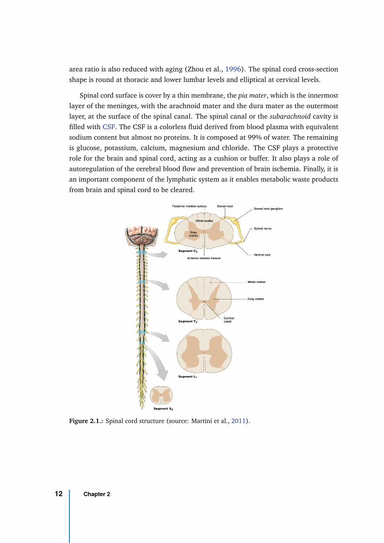
area ratio is also reduced with aging (Zhou et al., 1996). The spinal cord cross-section

shape is round at thoracic and lower lumbar levels and elliptical at cervical levels.

Spinal cord surface is cover by a thin membrane, the pia mater, which is the innermost

layer of the meninges, with the arachnoid mater and the dura mater as the outermost

layer, at the surface of the spinal canal. The spinal canal or the subarachnoid cavity is

filled with CSF. The CSF is a colorless fluid derived from blood plasma with equivalent

sodium content but almost no proteins. It is composed at 99% of water. The remaining

is glucose, potassium, calcium, magnesium and chloride. The CSF plays a protective

role for the brain and spinal cord, acting as a cushion or buffer. It also plays a role of

autoregulation of the cerebral blood flow and prevention of brain ischemia. Finally, it is

an important component of the lymphatic system as it enables metabolic waste products

from brain and spinal cord to be cleared.

Figure 2.1.: Spinal cord structure (source: Martini et al., 2011).

12 Chapter 2

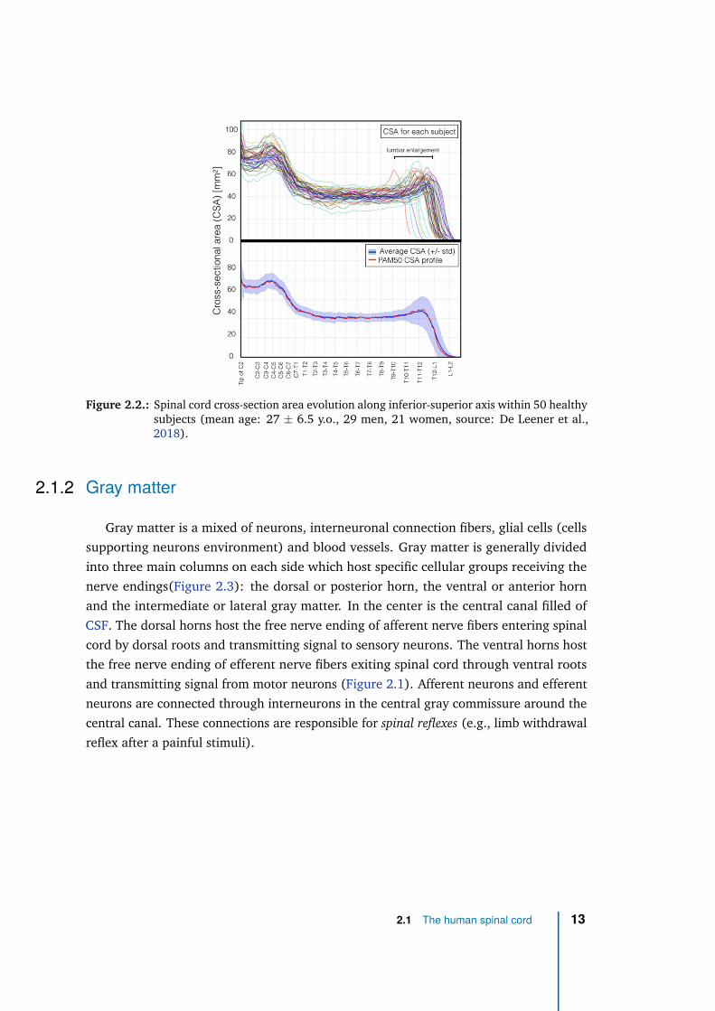
Figure 2.2.: Spinal cord cross-section area evolution along inferior-superior axis within 50 healthysubjects (mean age: 27 ± 6.5 y.o., 29 men, 21 women, source: De Leener et al.,2018).

2.1.2 Gray matter

Gray matter is a mixed of neurons, interneuronal connection fibers, glial cells (cells

supporting neurons environment) and blood vessels. Gray matter is generally divided

into three main columns on each side which host specific cellular groups receiving the

nerve endings(Figure 2.3): the dorsal or posterior horn, the ventral or anterior horn

and the intermediate or lateral gray matter. In the center is the central canal filled of

CSF. The dorsal horns host the free nerve ending of afferent nerve fibers entering spinal

cord by dorsal roots and transmitting signal to sensory neurons. The ventral horns host

the free nerve ending of efferent nerve fibers exiting spinal cord through ventral roots

and transmitting signal from motor neurons (Figure 2.1). Afferent neurons and efferent

neurons are connected through interneurons in the central gray commissure around the

central canal. These connections are responsible for spinal reflexes (e.g., limb withdrawal

reflex after a painful stimuli).

2.1 The human spinal cord 13

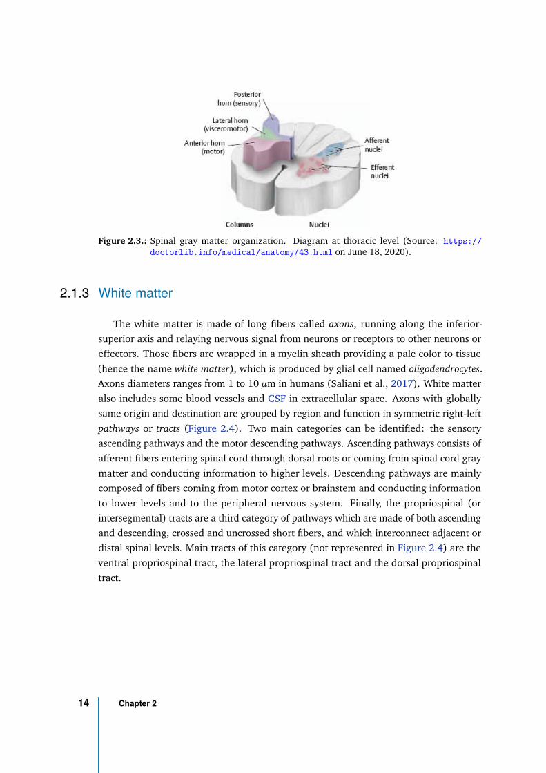
Figure 2.3.: Spinal gray matter organization. Diagram at thoracic level (Source: https://

doctorlib.info/medical/anatomy/43.html on June 18, 2020).

2.1.3 White matter

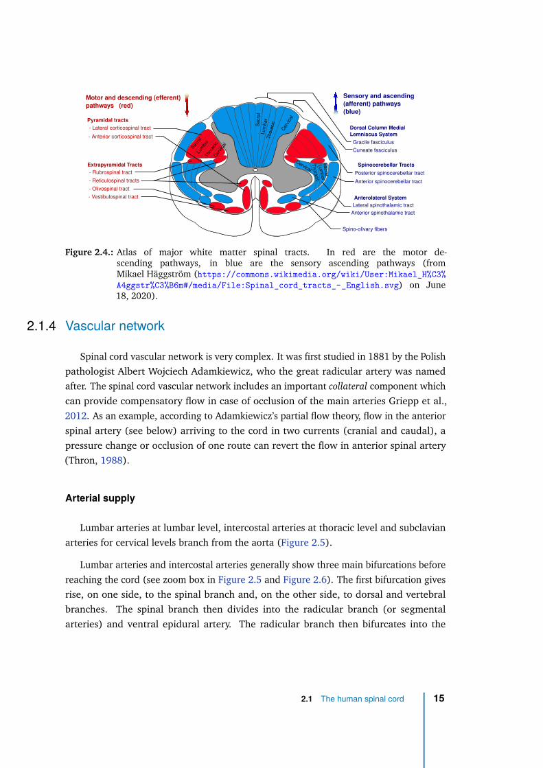
The white matter is made of long fibers called axons, running along the inferior-

superior axis and relaying nervous signal from neurons or receptors to other neurons or

effectors. Those fibers are wrapped in a myelin sheath providing a pale color to tissue

(hence the name white matter), which is produced by glial cell named oligodendrocytes.

Axons diameters ranges from 1 to 10 µm in humans (Saliani et al., 2017). White matter

also includes some blood vessels and CSF in extracellular space. Axons with globally

same origin and destination are grouped by region and function in symmetric right-left

pathways or tracts (Figure 2.4). Two main categories can be identified: the sensory

ascending pathways and the motor descending pathways. Ascending pathways consists of

afferent fibers entering spinal cord through dorsal roots or coming from spinal cord gray

matter and conducting information to higher levels. Descending pathways are mainly

composed of fibers coming from motor cortex or brainstem and conducting information

to lower levels and to the peripheral nervous system. Finally, the propriospinal (or

intersegmental) tracts are a third category of pathways which are made of both ascending

and descending, crossed and uncrossed short fibers, and which interconnect adjacent or

distal spinal levels. Main tracts of this category (not represented in Figure 2.4) are the

ventral propriospinal tract, the lateral propriospinal tract and the dorsal propriospinal

tract.

14 Chapter 2

https://doctorlib.info/medical/anatomy/43.html

https://doctorlib.info/medical/anatomy/43.html

Sensory and ascending

(afferent) pathways

(blue)

Motor and descending (efferent)

pathways (red)

Sac

ral

Lum

bar

Tho

raci

cC

ervi

cal

Sacra

lLum

bar

Cer

vica

l

Thora

cic

- Lateral corticospinal tract

Extrapyramidal Tracts

- Rubrospinal tract

- Reticulospinal tracts

- Vestibulospinal tract

- Olivospinal tract

- Anterior corticospinal tract

Pyramidal tracts

Dorsal Column Medial

Lemniscus System

Gracile fasciculus

Cuneate fasciculus

Spinocerebellar Tracts

Posterior spinocerebellar tract

Anterior spinocerebellar tract

Anterolateral System

Lateral spinothalamic tract

Anterior spinothalamic tract

Spino-olivary fibers

Sacra

l

Lum

bar

Thora

cic

Cervical

Figure 2.4.: Atlas of major white matter spinal tracts. In red are the motor de-scending pathways, in blue are the sensory ascending pathways (fromMikael Häggström (https://commons.wikimedia.org/wiki/User:Mikael_H%C3%

A4ggstr%C3%B6m#/media/File:Spinal_cord_tracts_-_English.svg) on June18, 2020).

2.1.4 Vascular network

Spinal cord vascular network is very complex. It was first studied in 1881 by the Polish

pathologist Albert Wojciech Adamkiewicz, who the great radicular artery was named

after. The spinal cord vascular network includes an important collateral component which

can provide compensatory flow in case of occlusion of the main arteries Griepp et al.,

2012. As an example, according to Adamkiewicz’s partial flow theory, flow in the anterior

spinal artery (see below) arriving to the cord in two currents (cranial and caudal), a

pressure change or occlusion of one route can revert the flow in anterior spinal artery

(Thron, 1988).

Arterial supply

Lumbar arteries at lumbar level, intercostal arteries at thoracic level and subclavian

arteries for cervical levels branch from the aorta (Figure 2.5).

Lumbar arteries and intercostal arteries generally show three main bifurcations before

reaching the cord (see zoom box in Figure 2.5 and Figure 2.6). The first bifurcation gives

rise, on one side, to the spinal branch and, on the other side, to dorsal and vertebral

branches. The spinal branch then divides into the radicular branch (or segmental

arteries) and ventral epidural artery. The radicular branch then bifurcates into the


https://commons.wikimedia.org/wiki/User:Mikael_H%C3%A4ggstr%C3%B6m#/media/File:Spinal_cord_tracts_-_English.svg

https://commons.wikimedia.org/wiki/User:Mikael_H%C3%A4ggstr%C3%B6m#/media/File:Spinal_cord_tracts_-_English.svg

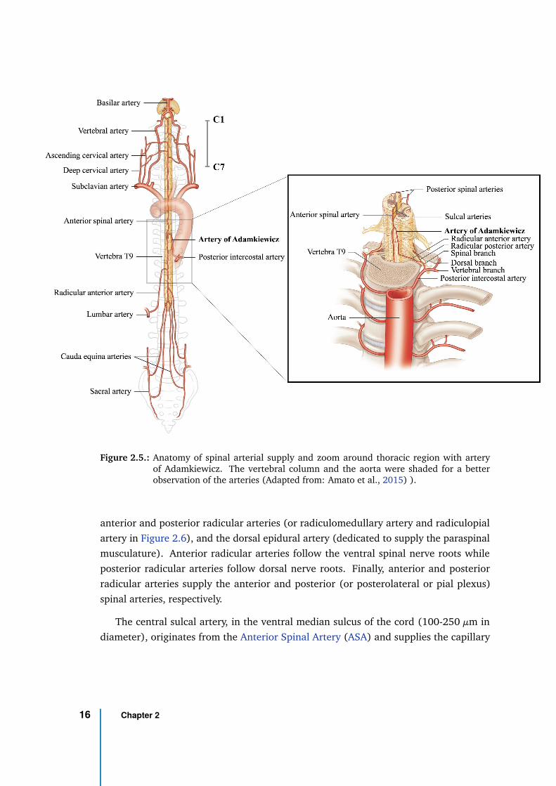
Figure 2.5.: Anatomy of spinal arterial supply and zoom around thoracic region with arteryof Adamkiewicz. The vertebral column and the aorta were shaded for a betterobservation of the arteries (Adapted from: Amato et al., 2015) ).

anterior and posterior radicular arteries (or radiculomedullary artery and radiculopial

artery in Figure 2.6), and the dorsal epidural artery (dedicated to supply the paraspinal

musculature). Anterior radicular arteries follow the ventral spinal nerve roots while

posterior radicular arteries follow dorsal nerve roots. Finally, anterior and posterior

radicular arteries supply the anterior and posterior (or posterolateral or pial plexus)

spinal arteries, respectively.

The central sulcal artery, in the ventral median sulcus of the cord (100-250 µm in

diameter), originates from the Anterior Spinal Artery (ASA) and supplies the capillary

16 Chapter 2

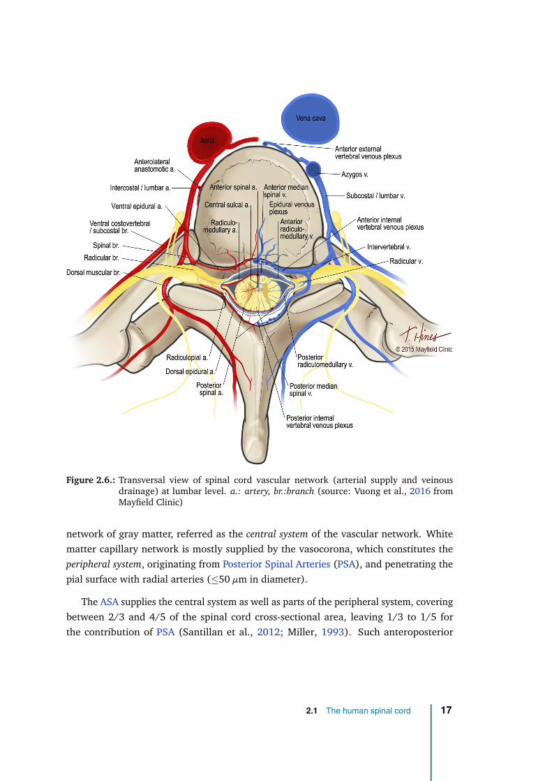
Figure 2.6.: Transversal view of spinal cord vascular network (arterial supply and veinousdrainage) at lumbar level. a.: artery, br.:branch (source: Vuong et al., 2016 fromMayfield Clinic)

network of gray matter, referred as the central system of the vascular network. White

matter capillary network is mostly supplied by the vasocorona, which constitutes the

peripheral system, originating from Posterior Spinal Arteries (PSA), and penetrating the

pial surface with radial arteries (≤50 µm in diameter).

The ASA supplies the central system as well as parts of the peripheral system, covering

between 2/3 and 4/5 of the spinal cord cross-sectional area, leaving 1/3 to 1/5 for

the contribution of PSA (Santillan et al., 2012; Miller, 1993). Such anteroposterior


asymmetry explains the difference in artery diameters, 200-500 µm for the ASA versus

100-200 µm for PSA.

At lower thoracic levels, although 4-6 radiculomedullary arteries can exist, there is

most often a single dominant one (the artery of Adamkiewicz, see Figure 2.5), which

arises between T8 and L3 vertebral levels (most usually at T9) and on the left side for

80% of subjects. This right-left asymmetry likely comes from the position of the aorta

on the left side of the spine and natural selection of shorter radiculomedullary arteries.

In upper thoracic region, around 70% of subjects present a dominant radiculomedullary

artery between left T3 and T7 vertebral levels (artery of Von Haller) (Gailloud et al.,

2014). In around 15% of subjects, when the dominant radiculomedullary artery arises

above T8, an additional one is present between L1 and L3 (artery if the conus medullaris),

deriving from the spinal branch of a lumbar artery.

At cervical levels, the subclavian artery supplies the deep cervical artery, the ascending

cervical artery and the vertebral artery. Deep cervical and ascending cervical arteries

merge and finally join the vertebral artery to supply typically one or two radiculomedullary

arteries in the cervical enlargement region. A dominant radiculomedullary artery is

usually present at C3 with possibly additional accessory ones around C6 and/or C8. In

upper cervical region, ASA and PSA are mostly supplied by branches of the vertebral

arteries (Figure 2.5). Note that vertebral arteries, ASA and PSA are mostly oriented

along inferior-superior axis while radiculomedullary arteries and radiculopial arteries are

mostly in the transverse plane to spinal cord.

Venous drainage

Intrinsic venous drainage system of the spinal cord is symmetric and centrifugal.

The deep central regions of the cord (mostly gray matter) are drained symmetrically by

anterior and posterior median spinal veins from the center to the periphery (Figure 2.6).

Peripheral regions (mostly white matter) are drained by radial veins centrifugally into the

coronal venous plexus on the pia matter surface, which connect to median spinal veins.

Similarly to the arterial supply network, anterior and posterior median spinal veins

then empty into ventral and radiculomedullary veins (or radicular veins) at the level of

spinal nerve roots. Similar to radiculomedullary arteries, radicular veins are substantial

at a limited number of vertebral segment (5-10 anteriorly, 5-10 posteriorly). Radicular

veins then drain into segmental spinal veins (intervertebral veins). Those segmental

18 Chapter 2

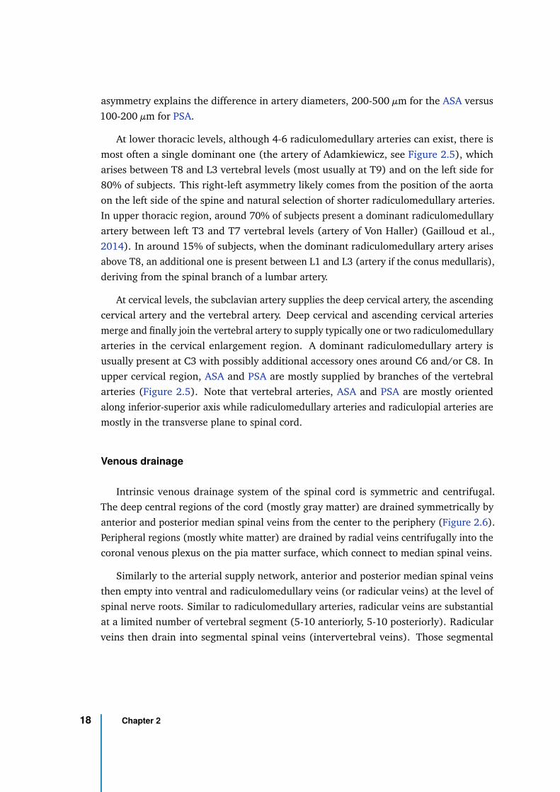
spinal veins then empty into subcostal or lumbar veins that then reach the azygos vessels

which finally drain into the venous cava. In the thoracic region, there are three azygos

vessels: the azygos vein on the right, the hemiazygos vein and the accessory hemiazygos

vein on the left (Figure 2.7). All of them drain into the superior venous cava.

Figure 2.7.: Anatomy of spinal venous drainage (Adapted from: Santillan et al., 2012 and Amatoet al., 2015).

At cervical levels, radiculomedullary veins and then segmental veins drain into verte-

bral veins which then empty in the subclavian veins either directly or via the deep cervical

veins. The subclavian vein finally drains in the superior vena cava (Figure 2.7).

2.2 Magnetic Resonance Imaging acquisition

This section describes where the Nuclear Magnetic Resonance (NMR) signal arises

from and how it is recorded. The methods to reconstruct an image from this signal is

2.2 Magnetic Resonance Imaging acquisition 19

then explained and rapid MRI acquisition strategies are then introduced as they are of

great interest for perfusion imaging.

2.2.1 Nuclear Magnetic Resonance signal

Nuclear spin

In quantum mechanics, the spin angular momentum ~S (or spin) is an intrinsic property

of any elementary particle (Levitt, 2001). It is a type of angular momentum but it is

not produced by a rotation of the particle as the rotational angular momentum J. Each

elementary particle has a particular spin value given by the spin quantum number s. This

number defines the number of states of the particle (2s+1). In the absence of an external

magnetic field, all states have the same energy level, they are said degenerate. An external

magnetic field breaks the degeneracy and assign to each state a different energy level.

The splitting between those levels is called the Zeeman splitting).

Nuclear Magnetic Resonance (NMR) can occur with atomic nuclei of non-null spin

quantum number (s 6= 0). Fortunately, multiple nuclei in the human body have a non-

null spin (e.g., hydrogen, sodium, phosphorus). Given its large natural abundance in

the human body (60% of water, H2O), Magnetic Resonance Imaging (MRI) is largely

performed based on the hydrogen nucleus 1H or proton (s = 12), and MRI based on other

types of nucleus is called X-nuclei MRI.

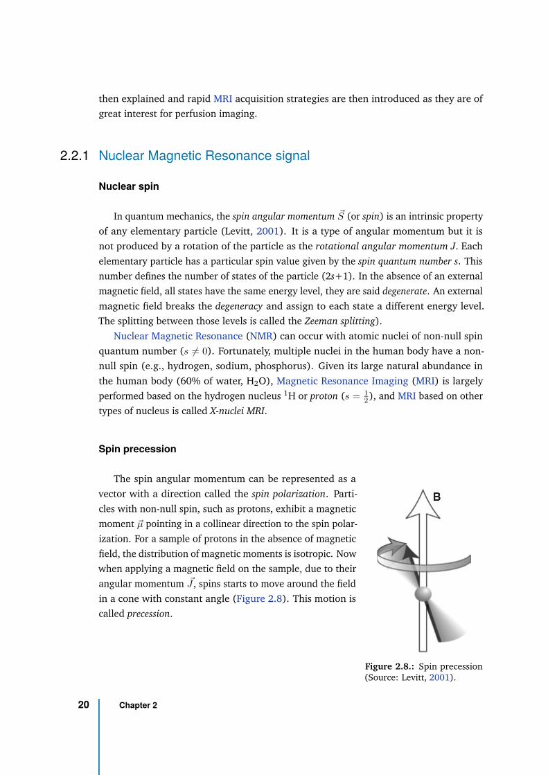
Spin precession

Figure 2.8.: Spin precession(Source: Levitt, 2001).

The spin angular momentum can be represented as a

vector with a direction called the spin polarization. Parti-

cles with non-null spin, such as protons, exhibit a magnetic

moment ~µ pointing in a collinear direction to the spin polar-

ization. For a sample of protons in the absence of magnetic

field, the distribution of magnetic moments is isotropic. Now

when applying a magnetic field on the sample, due to their

angular momentum ~J , spins starts to move around the field

in a cone with constant angle (Figure 2.8). This motion is

called precession.

20 Chapter 2

The frequency of precession ω0 = 2πf0 (in radians/s and f0 the frequency in Hz)

depends on the magnetic field amplitude B0 and the gyromagnetic ratio defined as γ = Jµ .

For nuclear spins, this frequency of precession is called the nuclear Larmor frequency and

is:

ω0 = −γB0

Most nuclei have a positive gyromagnetic ratio (267.52 × 106 rad/s/T or 42.58 MHz/Tesla

for 1H), meaning their spins precess in the clockwise direction around B0 (the counter-

clockwise direction being defined positive by convention) (Levitt, 2001).

The proton Larmor frequency (absolute value) therefore equals 802.61 × 106 rad/s or

127.74 MHz at 3T and 1872.77 × 106 rad/s or 298.06 MHz at 7T.

Magnetization

In the human body, free protons are mostly found within the water molecules H2O.

The 1H nucleus has spin quantum number of 12 , thus two energy levels are possible

(Zeeman effect): ms = +s = 12 (spin-up) or ms = −s = −1

2 (spin-down). The energy

difference is ∆E = ~ω0 = ~γB0 (with ~ = h/2π =1.38 × 10−34 the reduced Planck’s

constant) and therefore depends on the field strength.

In absence of a magnetic field, the macroscopic magnetic moment of the sample (sum

of all spins magnetic moment, ~Mequilibrium =∑

spins ~µi, called the magnetization) is close

to 0 (isotropic distribution of the spins polarization).

In the presence of a magnetic fields, the protons’ molecular environment add micro-

scopic magnetic fields fluctuating due to thermal agitation at the human body temperature.

Protons therefore experience a total magnetic field slightly fluctuating in amplitude and

direction. A system of spins in a magnetic field then follows a Boltzmann distribution

where the states with lower energy (spin-up) have a slightly higher probability of being

occupied, according to:N+

N−= e−∆E/kT

where N+ and N− are the number of spins in the higher (spin-down) and lower (spin-

up) energy states, k=1.38 × 10−23 J/K is Boltzmann’s constant and T is the temperature

(310 K in the human body). Instead of having all spins magnetic moment aligned in the

direction of the magnetic field, these fluctuations induce an anisotropic distribution of

the spins polarization, with a slightly higher probability for the configuration with lower


magnetic energy, i.e. with the spins magnetic moment aligned in the direction of the

magnetic field.

The probability of finding a spin within the system with energy ǫ is:

P (ǫ) =e−ǫ/kT

∑ǫ

e−ǫ/kT(2.1)

The net magnetization of the system at equilibrium is the sum of individual magnetizations

that is:

M0 = ρ0

∑

ms=s,−s

P (ǫ(ms))µ(ms) (2.2)

where ρ0 is the spin density, ǫ(ms) = −ms~ω0 is the energy for state ms and µ(ms) =

msγ~ is the magnetization for state ms, leading to:

M0 = ρ0γ~

∑ms=s,−s

msems~ω0

kT

∑ms=s,−s

ems~ω0

kT

= ρ0γ~

∑ms=s,−s

msemsu

∑ms=s,−s

emsu(2.3)

with u = ~ω0

kT . Since the nuclear magnetic energies are much smaller than the thermal

energies at the human body temperature, u << 1 , we have emsu ≈ 1 + msu (Taylor

expansion), simplifying to:

M0 =ρ0γ2

~2

4kTB0 (2.4)

The net magnetization amplitude therefore depends on the field strength B0, gyromag-

netic ratio γ, environment temperature T (in Kelvin) and proton density ρ0.

Longitudinal and transverse relaxations

Let us consider a sample of water molecules protons in the human body in a magnet

with magnetic field ~B0 = B0~z. The macroscopic net magnetization is aligned in the

direction of the field (~z), with spins precessing around this direction at the Larmor

frequency at the microscopic scale. This magnetization is called longitudinal magnetization~Mz.

The longitudinal magnetization is almost undetectable. The NMR strategy is to measure

it in the perpendicular plane to the field.

22 Chapter 2

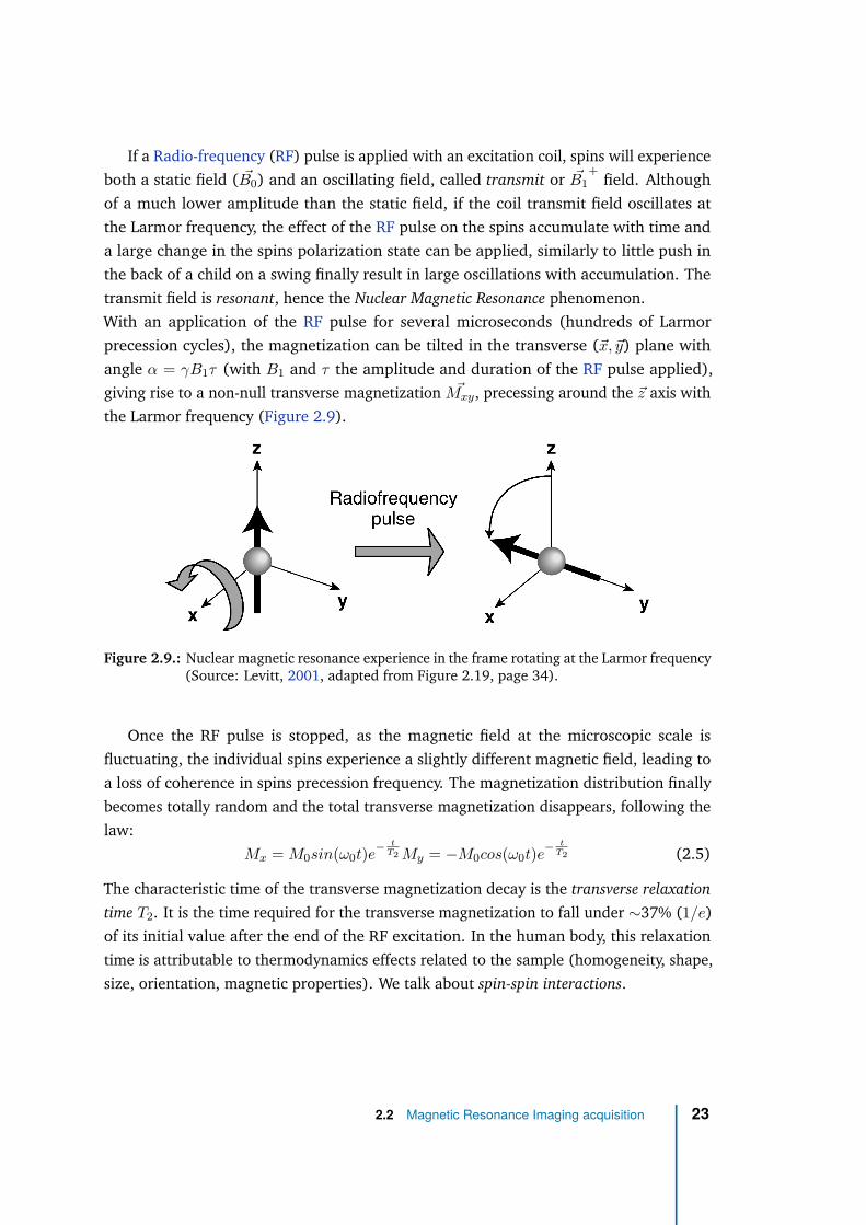
If a Radio-frequency (RF) pulse is applied with an excitation coil, spins will experience

both a static field ( ~B0) and an oscillating field, called transmit or ~B1+

field. Although

of a much lower amplitude than the static field, if the coil transmit field oscillates at

the Larmor frequency, the effect of the RF pulse on the spins accumulate with time and

a large change in the spins polarization state can be applied, similarly to little push in

the back of a child on a swing finally result in large oscillations with accumulation. The

transmit field is resonant, hence the Nuclear Magnetic Resonance phenomenon.

With an application of the RF pulse for several microseconds (hundreds of Larmor

precession cycles), the magnetization can be tilted in the transverse (~x, ~y) plane with

angle α = γB1τ (with B1 and τ the amplitude and duration of the RF pulse applied),

giving rise to a non-null transverse magnetization ~Mxy, precessing around the ~z axis with

the Larmor frequency (Figure 2.9).

Figure 2.9.: Nuclear magnetic resonance experience in the frame rotating at the Larmor frequency(Source: Levitt, 2001, adapted from Figure 2.19, page 34).

Once the RF pulse is stopped, as the magnetic field at the microscopic scale is

fluctuating, the individual spins experience a slightly different magnetic field, leading to

a loss of coherence in spins precession frequency. The magnetization distribution finally

becomes totally random and the total transverse magnetization disappears, following the

law:

Mx = M0sin(ω0t)e−

tT2 My = −M0cos(ω0t)e

−t

T2 (2.5)

The characteristic time of the transverse magnetization decay is the transverse relaxation

time T2. It is the time required for the transverse magnetization to fall under ∼37% (1/e)

of its initial value after the end of the RF excitation. In the human body, this relaxation

time is attributable to thermodynamics effects related to the sample (homogeneity, shape,

size, orientation, magnetic properties). We talk about spin-spin interactions.


Local field inhomogeneities, related to the system (field non-uniformity, shimming), add

to the spins loss in frequency coherence. This process is associated with the time constant

T ′

2 and results in an apparent relaxation with time T ∗

2 (< T2) according to:

1

T2=

1

T ∗

2

+1

T ′

2

(2.6)

While the spins get out of phase in the transverse plan, the spin distribution progressively

comes back to equilibrium along the static ~B0 field and the longitudinal magnetization

growths until recovering its initial amplitude, according to:

Mz = M0(1 − e−

tT1 ) (2.7)

The characteristic time of the longitudinal magnetization recovery is the longitudinal

relaxation time T1. It is the time required for the longitudinal magnetization to regrow at

∼63% (1 − 1/e) of its initial value after the end of the RF excitation. In the human body,

this relaxation time is attributable to interactions between spins and their environment

(spin-lattice interactions).

In living tissue, T1 ranges from around 100 to 4500 ms while T2 ranges from around

20 (excluding ultra-short T2 components) to 2000 ms.

Equation (2.5) and Equation (2.7) were established by Felix Bloch as a result of his

famous experiment on “Nuclear inducion” (Bloch, 1946; Block et al., 1946). Note that T1

and T2 were defined phenomenologically and not derived from fundamental principles.

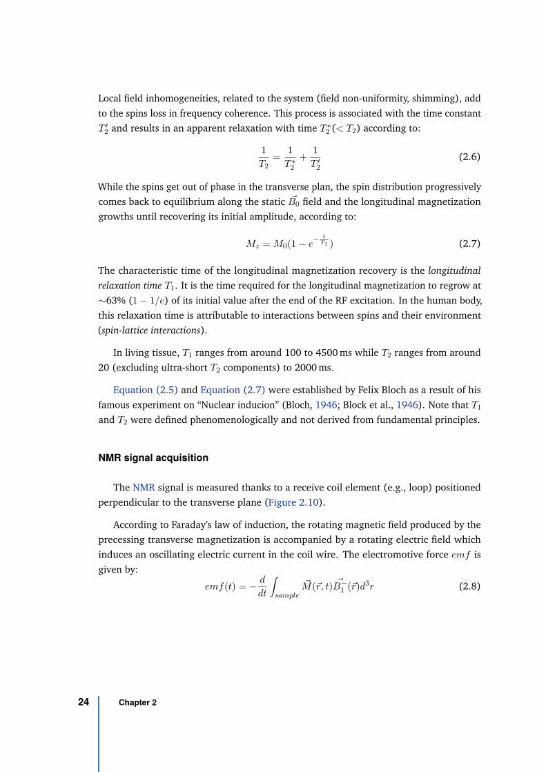
NMR signal acquisition

The NMR signal is measured thanks to a receive coil element (e.g., loop) positioned

perpendicular to the transverse plane (Figure 2.10).

According to Faraday’s law of induction, the rotating magnetic field produced by the

precessing transverse magnetization is accompanied by a rotating electric field which

induces an oscillating electric current in the coil wire. The electromotive force emf is

given by:

emf(t) = − d

dt

∫

sample

~M(~r, t) ~B−

1 (~r)d3r (2.8)

24 Chapter 2

Figure 2.10.: NMR signal acquisition (Source: Levitt, 2001, adapted from Figure 2.23, page 36).

where ~M is the net magnetization and ~B−

1 is the "receive" field of the detection coil,

which is the magnetic field per unit current that would be produced by the detection coil

(reciprocal principle). The oscillating current induced in the coil by the ~M after an RF

excitation pulse was applied, measures the NMR signal, also called the Free-Induction

Decay (FID). Although this current is very low, it can be detected using an RF detector

thanks to its well-known frequency.

Bloch’s equations as a function of time t and position ~r for a series of pulses are:

Mz(~r, t) = Mz(~r, t = 0)e−t/T1(~r) + M0(1 − e−t/T1(~r)) Mz(∞) = M0 (2.9)

Mxy(~r, t) = Mxy(~r, t = 0)e−t/T2(~r)e−i(ω0t+φ0(~r)) Mxy(∞) = 0 (2.10)

The magnitude Mxy(~r, t = 0) and phase φ0(~r) of the transverse magnetization are

determined by the RF pulse conditions at t = 0.

Feeding Equation (2.9) into Equation (2.8) and after further manipulations and

simplifications (especially knowing that ω0 is at least four order of magnitude larger than

1/T1 and 1/T2 for B0 around 1 T, allowing the derivative of the e1/T1(~r) and e1/T2(~r) to be

neglected), it can be shown that (Haacke et al. (1999), chapter 7.3):

signalemf (t) ∝ ω0

∫

samplee−t/T2(~r)Mxy(~r, t = 0)B−

1,xy(~r)sin(ω0t + θB−

1

(~r) − φ0(~r))d3r

(2.11)


where Mxy and B−

1,xy are the transverse components of the magnetization and receive

field, and θB−

1

is the angle between the receive field and the magnetization. The signal is

then demodulated into two channels, called the real and imaginary channel, multiplying

signalemf by a reference signal, sin(ω0 + δω)t for the real channel and −cos(ω0 + δω)t

for the imaginary channel. After filtering of the high frequency component (2ω0 + δω),

we obtain the complex demodulated signal:

signaldemodulated ∝ ω0

∫

samplee−t/T2(~r)Mxy(~r, t = 0)B−

1,xy(~r)ei((Ω−ω0)t−θ

B−

1

(~r)+φ0(~r))d3r

(2.12)

with Ω the frequency of the reference signal used for demodulation (most often set to

ω0 + δω).

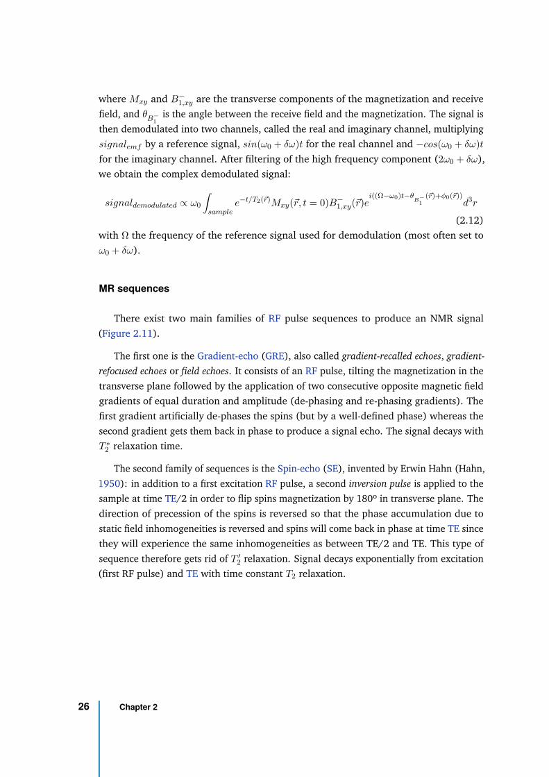
MR sequences

There exist two main families of RF pulse sequences to produce an NMR signal

(Figure 2.11).

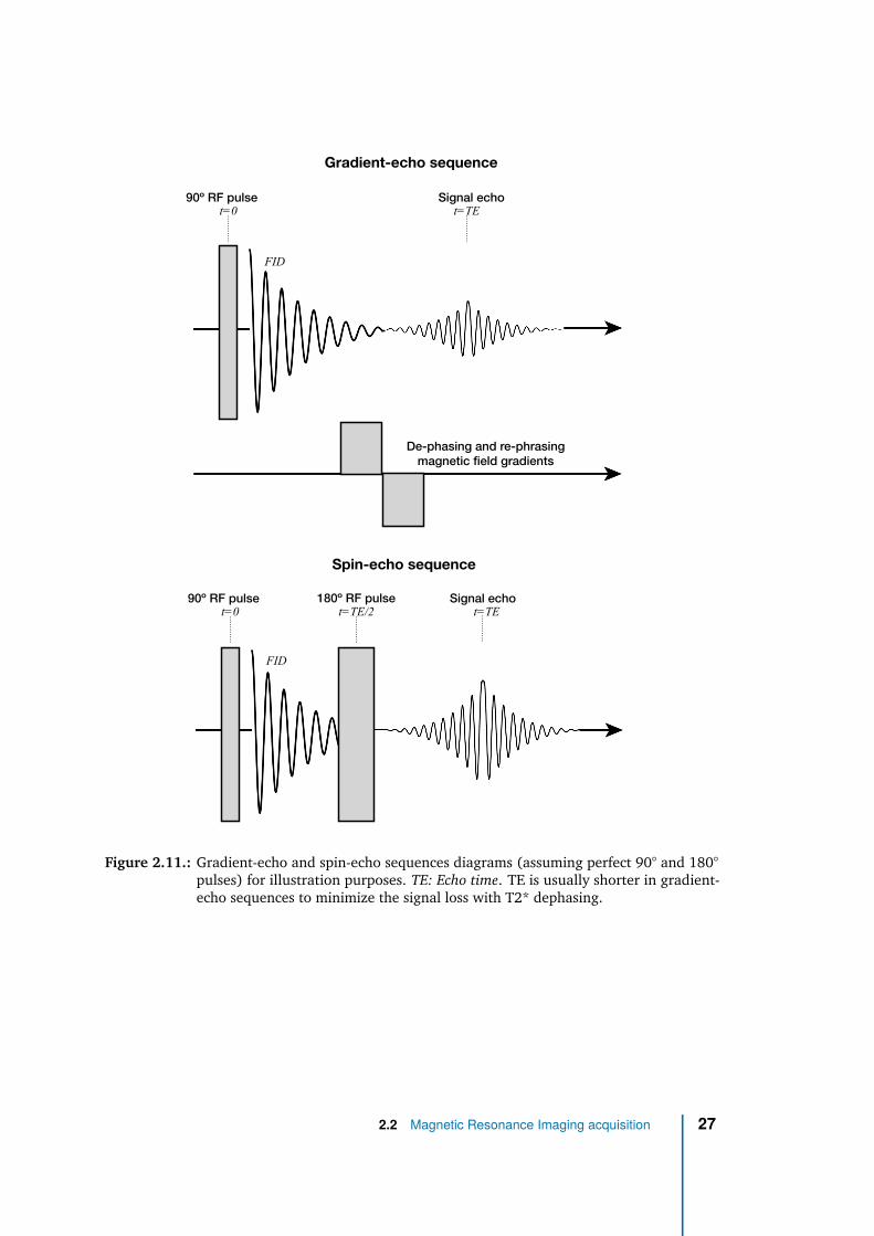
The first one is the Gradient-echo (GRE), also called gradient-recalled echoes, gradient-

refocused echoes or field echoes. It consists of an RF pulse, tilting the magnetization in the

transverse plane followed by the application of two consecutive opposite magnetic field

gradients of equal duration and amplitude (de-phasing and re-phasing gradients). The

first gradient artificially de-phases the spins (but by a well-defined phase) whereas the

second gradient gets them back in phase to produce a signal echo. The signal decays with

T ∗

2 relaxation time.

The second family of sequences is the Spin-echo (SE), invented by Erwin Hahn (Hahn,

1950): in addition to a first excitation RF pulse, a second inversion pulse is applied to the

sample at time TE/2 in order to flip spins magnetization by 180º in transverse plane. The

direction of precession of the spins is reversed so that the phase accumulation due to

static field inhomogeneities is reversed and spins will come back in phase at time TE since

they will experience the same inhomogeneities as between TE/2 and TE. This type of

sequence therefore gets rid of T ′

2 relaxation. Signal decays exponentially from excitation

(first RF pulse) and TE with time constant T2 relaxation.

26 Chapter 2

90º RF pulse Signal echot=0 t=TE

90º RF pulse Signal echot=0 t=TEt=TE/2

Gradient-echo sequence

Spin-echo sequence

180º RF pulse

De-phasing and re-phrasing

magnetic field gradients

FID

FID

Figure 2.11.: Gradient-echo and spin-echo sequences diagrams (assuming perfect 90° and 180°pulses) for illustration purposes. TE: Echo time. TE is usually shorter in gradient-echo sequences to minimize the signal loss with T2* dephasing.


2.2.2 Image acquisition and reconstruction

For Magnetic Resonance Imaging, it is necessary to encode the signal as a function

of the position in space. Only the concepts used in this PhD work and/or relevant to its

discussion will be introduced here. More details can be found in the excellent books from

Levitt (2001) or Haacke et al. (1999).

K-space

Spatial encoding It is possible to encode the signal as a function of the spins position ~r

with the use of magnetic field gradients ~G(t).

If we consider the transmitting and receiving RF coil fields sufficiently uniform in

Equation (2.12), the initial phase φ0, the receiving RF coil field directional phase θB−

1

and transverse amplitude B−

1,xy can be assumed independent from the position. To turn

Equation (2.12) from proportionality to equality, all gain factors from the electronic

detection system can be included in a constant factor Λ. In addition, the constant

phases φ0 and θB−

1

can be set to 0 with loss of generality. The demodulated signal can

consequently be expressed as:

s(t) = ω0ΛB−

1,xy

∫ +∞

−∞

e−t/T2(~r)Mxy(~r, t = 0)ei(Ωt+φ(~r,t))d3r (2.13)

with Ω the demodulation frequency and φ(~r, t) = −∫ t

0 ω(~r, t′)dt′ is the accumulated phase

with time. Here, we assume that variation of φ with position is only due to a magnetic

field gradient ~G(t) and if ~G(t) = 0, φ(~r, t) = −ω0t as the static field is considered

homogeneous.

For clarity purpose, the relaxation effects can be ignored and we can define the « effective

» spin density ρ(~r) = ω0ΛB−

1,xyMxy(~r, t = 0) such that:

s(t) =

∫ +∞

−∞

ρ(~r)ei(Ωt+φ(~r,t))d3r (2.14)

The goal of MR imaging is to measure the spin density as a function of the position to form

an image of the object. Let us now consider the effect of a magnetic field gradient in one

dimension ~x: ~G(t) = Gx(t)~x = ∂Bx

∂x (t)~x. The 1D spin density is ρ(x) =∫

sample ρ(~r)dydz.

28 Chapter 2

Along ~x, the magnetic field varies linearly as a function of the position and so does the

frequency:

Bx(x, t) = B0 + xG(t) = B0 + xGx(t) (2.15)

ω(x, t) = ω0 + γxG(t) = ω0 + γxGx(t) (2.16)

The gradient is used to establish a relation between the spins position and their precession

rate. This technique is referred as frequency encoding. The accumulated phase up to time

t is therefore:

φ(~r, t) = −∫ t

0ω(~r, t′)dt′ = −ω0t − γx

∫ t

0Gx(t)dt (2.17)

With a frequency modulation Ω = ω0, we get following relation between the signal and

the spatial frequency:

s(kx(t)) =

∫ +∞

−∞

ρ(x)e−i2πkx(t)xdx (2.18)

with kx(t) = γ2π

∫ t0 Gx(t′)dt′ the spatial frequency. The effective spin density can then be

obtained by inverse Fourier transform which is the link between the frequency domain

(s(kx)) and the image domain (ρ(x)):

ρ(x) =

∫ +∞

−∞

s(kx)e+i2πkx(t)xdkx (2.19)

The expression of the signal as a function of the spatial frequencies induced by gradients

can be generalized to three dimensions:

s(kx, ky, kz) =

∫ +∞

−∞

ρ(x, y, z)e−i2π(kxx+kyy+kzz)dx dy dz = F [ρ(x, y, z)] (2.20)

ρ(x, y, z) =

∫ +∞

−∞

s(kx, ky, kz)ei2π(kxx+kyy+kzz)dkx dky dkz = F−1[s(kx, ky, kz)]

with kx(t) =γ

2π

∫ t

0Gx(t′)dt′ , ky(t) =

γ

2π

∫ t

0Gy(t′)dt′ and kz(t) =

γ

2π

∫ t

0Gz(t′)dt′

F and F−1 refer to the Fourier transform and the inverse Fourier transform.

To retrieve the spin density of the sample ρ(x, y, z) in three dimensions, it is therefore

necessary to measure s(kx, ky, kz) with (kx, ky, kz) ∈ [−∞; +∞]3. This domain is called

k-space while its inverse Fourier transform is often referred as the image space since it

provides an image of the effective spin density.


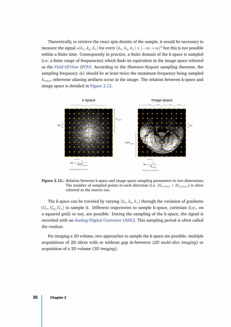
Theoretically, to retrieve the exact spin density of the sample, it would be necessary to

measure the signal s(kx, ky, kz) for every (kx, ky, kz) ∈ [−∞; +∞]3 but this is not possible

within a finite time. Consequently in practice, a finite domain of the k-space is sampled

(i.e. a finite range of frequencies) which finds its equivalent in the image space referred

as the Field-Of-View (FOV). According to the Shannon-Nyquist sampling theorem, the

sampling frequency ∆k should be at least twice the maximum frequency being sampled

kmax, otherwise aliasing artifacts occur in the image. The relation between k-space and

image space is detailed in Figure 2.12.

Δkx =1

2FOVx,max

k-space Image space

(kx, ky) ∈ [−kx,max; kx,max] × [−ky,max; ky,max]

Δx =1

2kx,max

(x, y) ∈ [−FOVx,max; FOVx,max] × [−FOVy,max; FOVy,max]

Δky

ky,max

FOVy,max

sampling frequency image resolution

Δy

Figure 2.12.: Relation between k-space and image space sampling parameters in two dimensions.The number of sampled points in each direction (i.e. 2kx,max × 2ky,max) is oftenreferred as the matrix size.

The k-space can be traveled by varying (kx, ky, kz) through the variation of gradients

(Gx, Gy, Gz) to sample it. Different trajectories to sample k-space, cartesian (i.e., on

a squared grid) or not, are possible. During the sampling of the k-space, the signal is

recorded with an Analog/Digital Converter (ADC). This sampling period is often called

the readout.

For imaging a 3D volume, two approaches to sample the k-space are possible: multiple

acquisitions of 2D slices with or without gap in-between (2D multi-slice imaging) or

acquisition of a 3D volume (3D imaging).

30 Chapter 2

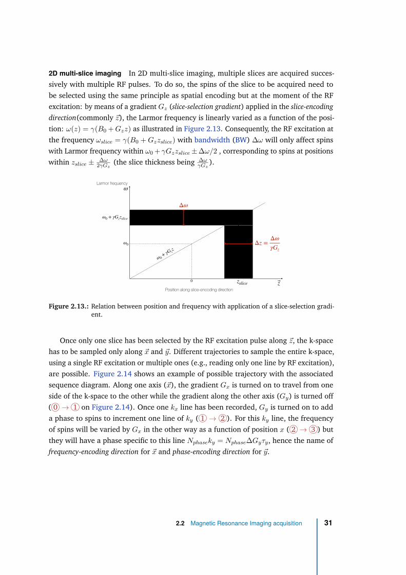
2D multi-slice imaging In 2D multi-slice imaging, multiple slices are acquired succes-

sively with multiple RF pulses. To do so, the spins of the slice to be acquired need to

be selected using the same principle as spatial encoding but at the moment of the RF

excitation: by means of a gradient Gz (slice-selection gradient) applied in the slice-encoding

direction(commonly ~z), the Larmor frequency is linearly varied as a function of the posi-

tion: ω(z) = γ(B0 + Gzz) as illustrated in Figure 2.13. Consequently, the RF excitation at

the frequency ωslice = γ(B0 + Gzzslice) with bandwidth (BW) ∆ω will only affect spins

with Larmor frequency within ω0 + γGzzslice ± ∆ω/2 , corresponding to spins at positions

within zslice ± ∆ω2γGz

(the slice thickness being ∆ωγGz

).

Position along slice-encoding direction

z

Larmor frequency

ω

zslice

ω 0+

γG zz

0

ω0 + γGzzslice

ω0

Δω

Δz =Δω

γGz

Figure 2.13.: Relation between position and frequency with application of a slice-selection gradi-ent.

Once only one slice has been selected by the RF excitation pulse along ~z, the k-space

has to be sampled only along ~x and ~y. Different trajectories to sample the entire k-space,

using a single RF excitation or multiple ones (e.g., reading only one line by RF excitation),

are possible. Figure 2.14 shows an example of possible trajectory with the associated

sequence diagram. Along one axis (~x), the gradient Gx is turned on to travel from one

side of the k-space to the other while the gradient along the other axis (Gy) is turned off

( 0 → 1 on Figure 2.14). Once one kx line has been recorded, Gy is turned on to add

a phase to spins to increment one line of ky ( 1 → 2 ). For this ky line, the frequency

of spins will be varied by Gx in the other way as a function of position x ( 2 → 3 ) but

they will have a phase specific to this line Nphaseky = Nphase∆Gyτy, hence the name of

frequency-encoding direction for ~x and phase-encoding direction for ~y.


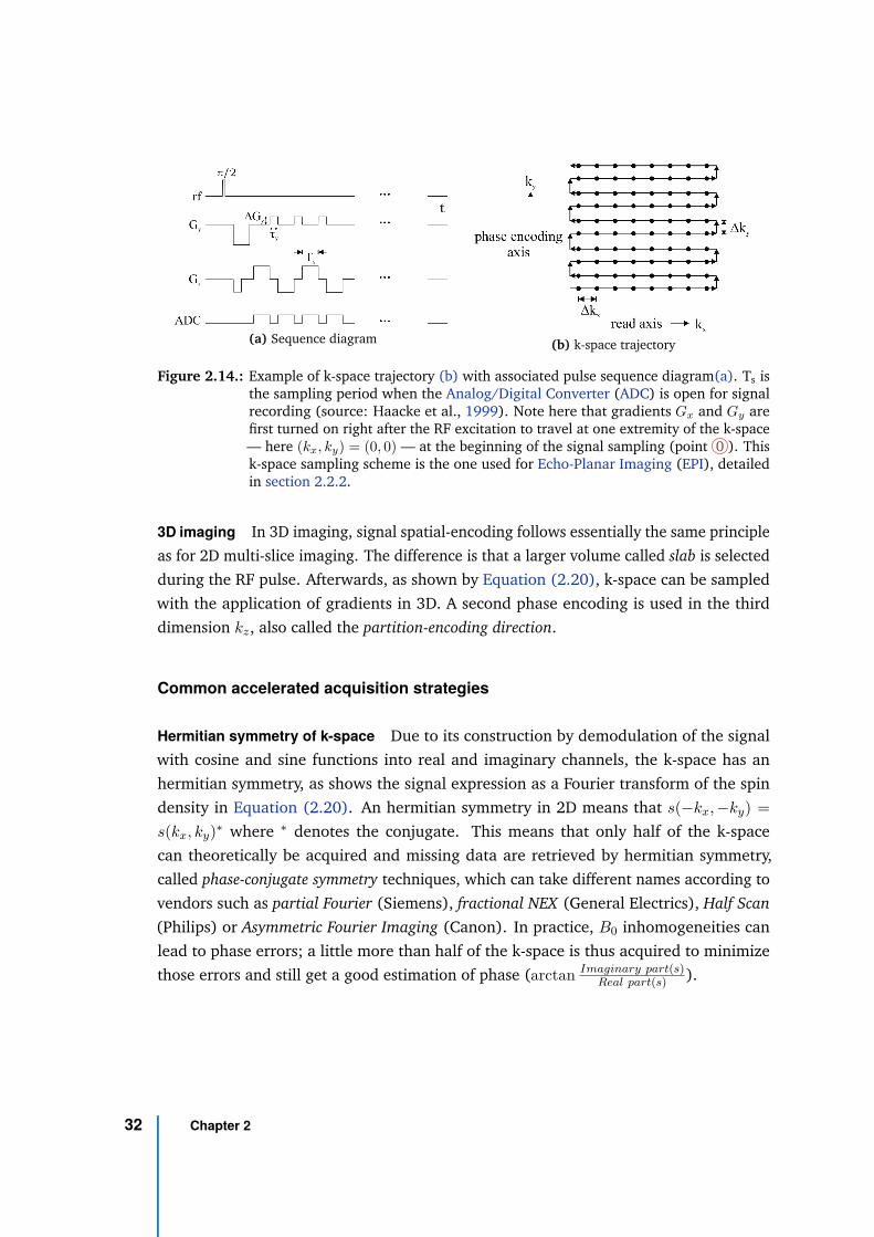
(a) Sequence diagram (b) k-space trajectory

Figure 2.14.: Example of k-space trajectory (b) with associated pulse sequence diagram(a). Ts isthe sampling period when the Analog/Digital Converter (ADC) is open for signalrecording (source: Haacke et al., 1999). Note here that gradients Gx and Gy arefirst turned on right after the RF excitation to travel at one extremity of the k-space— here (kx, ky) = (0, 0) — at the beginning of the signal sampling (point 0 ). Thisk-space sampling scheme is the one used for Echo-Planar Imaging (EPI), detailedin section 2.2.2.

3D imaging In 3D imaging, signal spatial-encoding follows essentially the same principle

as for 2D multi-slice imaging. The difference is that a larger volume called slab is selected

during the RF pulse. Afterwards, as shown by Equation (2.20), k-space can be sampled

with the application of gradients in 3D. A second phase encoding is used in the third

dimension kz, also called the partition-encoding direction.

Common accelerated acquisition strategies

Hermitian symmetry of k-space Due to its construction by demodulation of the signal

with cosine and sine functions into real and imaginary channels, the k-space has an

hermitian symmetry, as shows the signal expression as a Fourier transform of the spin

density in Equation (2.20). An hermitian symmetry in 2D means that s(−kx, −ky) =

s(kx, ky)∗ where ∗ denotes the conjugate. This means that only half of the k-space

can theoretically be acquired and missing data are retrieved by hermitian symmetry,

called phase-conjugate symmetry techniques, which can take different names according to

vendors such as partial Fourier (Siemens), fractional NEX (General Electrics), Half Scan

(Philips) or Asymmetric Fourier Imaging (Canon). In practice, B0 inhomogeneities can

lead to phase errors; a little more than half of the k-space is thus acquired to minimize

those errors and still get a good estimation of phase (arctan Imaginary part(s)Real part(s) ).

32 Chapter 2

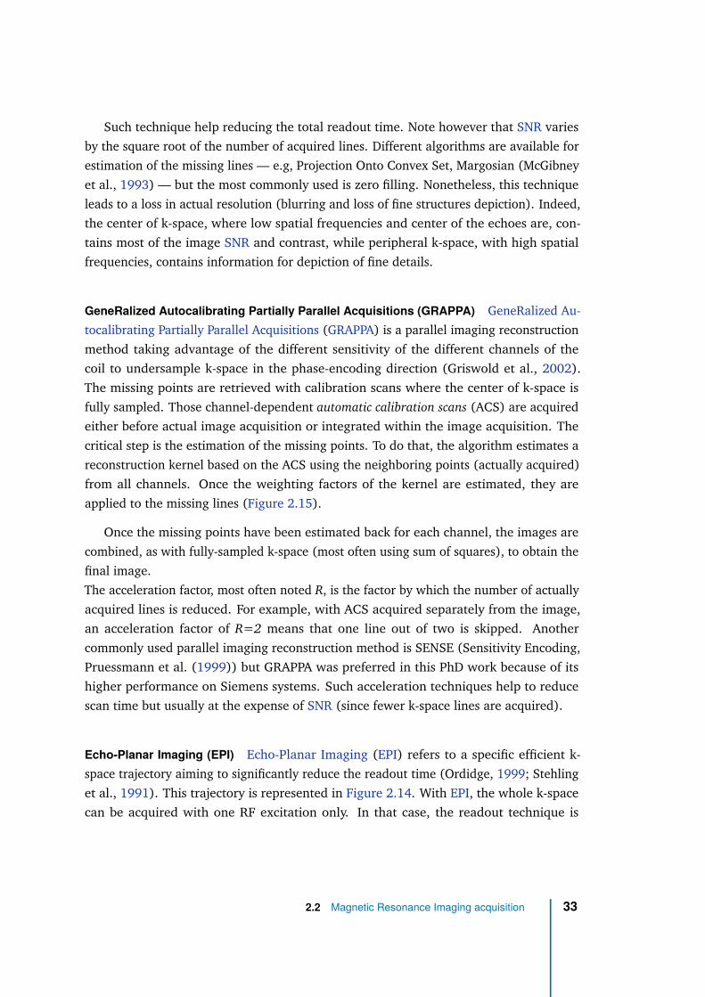
Such technique help reducing the total readout time. Note however that SNR varies

by the square root of the number of acquired lines. Different algorithms are available for

estimation of the missing lines — e.g, Projection Onto Convex Set, Margosian (McGibney

et al., 1993) — but the most commonly used is zero filling. Nonetheless, this technique

leads to a loss in actual resolution (blurring and loss of fine structures depiction). Indeed,

the center of k-space, where low spatial frequencies and center of the echoes are, con-

tains most of the image SNR and contrast, while peripheral k-space, with high spatial

frequencies, contains information for depiction of fine details.

GeneRalized Autocalibrating Partially Parallel Acquisitions (GRAPPA) GeneRalized Au-

tocalibrating Partially Parallel Acquisitions (GRAPPA) is a parallel imaging reconstruction

method taking advantage of the different sensitivity of the different channels of the

coil to undersample k-space in the phase-encoding direction (Griswold et al., 2002).

The missing points are retrieved with calibration scans where the center of k-space is

fully sampled. Those channel-dependent automatic calibration scans (ACS) are acquired

either before actual image acquisition or integrated within the image acquisition. The

critical step is the estimation of the missing points. To do that, the algorithm estimates a

reconstruction kernel based on the ACS using the neighboring points (actually acquired)

from all channels. Once the weighting factors of the kernel are estimated, they are

applied to the missing lines (Figure 2.15).

Once the missing points have been estimated back for each channel, the images are

combined, as with fully-sampled k-space (most often using sum of squares), to obtain the

final image.

The acceleration factor, most often noted R, is the factor by which the number of actually

acquired lines is reduced. For example, with ACS acquired separately from the image,

an acceleration factor of R=2 means that one line out of two is skipped. Another

commonly used parallel imaging reconstruction method is SENSE (Sensitivity Encoding,

Pruessmann et al. (1999)) but GRAPPA was preferred in this PhD work because of its

higher performance on Siemens systems. Such acceleration techniques help to reduce

scan time but usually at the expense of SNR (since fewer k-space lines are acquired).

Echo-Planar Imaging (EPI) Echo-Planar Imaging (EPI) refers to a specific efficient k-

space trajectory aiming to significantly reduce the readout time (Ordidge, 1999; Stehling

et al., 1991). This trajectory is represented in Figure 2.14. With EPI, the whole k-space

can be acquired with one RF excitation only. In that case, the readout technique is


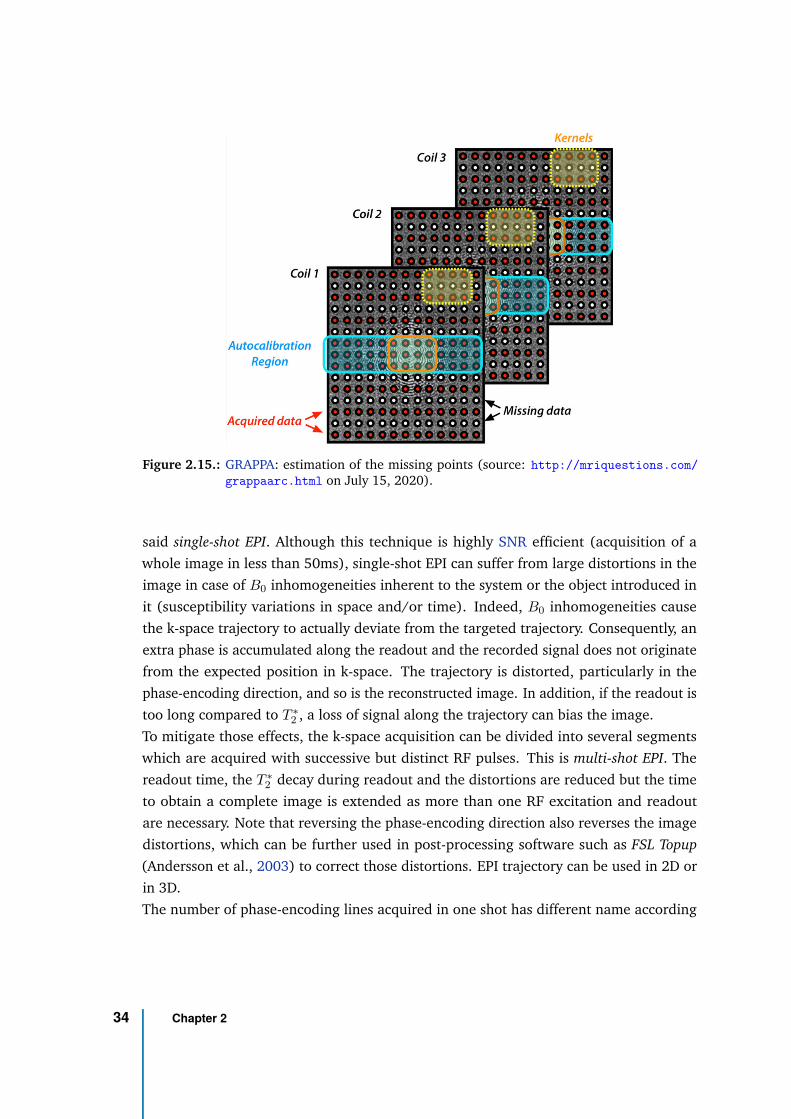
Figure 2.15.: GRAPPA: estimation of the missing points (source: http://mriquestions.com/

grappaarc.html on July 15, 2020).

said single-shot EPI. Although this technique is highly SNR efficient (acquisition of a

whole image in less than 50ms), single-shot EPI can suffer from large distortions in the

image in case of B0 inhomogeneities inherent to the system or the object introduced in

it (susceptibility variations in space and/or time). Indeed, B0 inhomogeneities cause

the k-space trajectory to actually deviate from the targeted trajectory. Consequently, an

extra phase is accumulated along the readout and the recorded signal does not originate

from the expected position in k-space. The trajectory is distorted, particularly in the

phase-encoding direction, and so is the reconstructed image. In addition, if the readout is

too long compared to T ∗

2 , a loss of signal along the trajectory can bias the image.

To mitigate those effects, the k-space acquisition can be divided into several segments

which are acquired with successive but distinct RF pulses. This is multi-shot EPI. The

readout time, the T ∗

2 decay during readout and the distortions are reduced but the time

to obtain a complete image is extended as more than one RF excitation and readout

are necessary. Note that reversing the phase-encoding direction also reverses the image

distortions, which can be further used in post-processing software such as FSL Topup

(Andersson et al., 2003) to correct those distortions. EPI trajectory can be used in 2D or

in 3D.

The number of phase-encoding lines acquired in one shot has different name according

34 Chapter 2

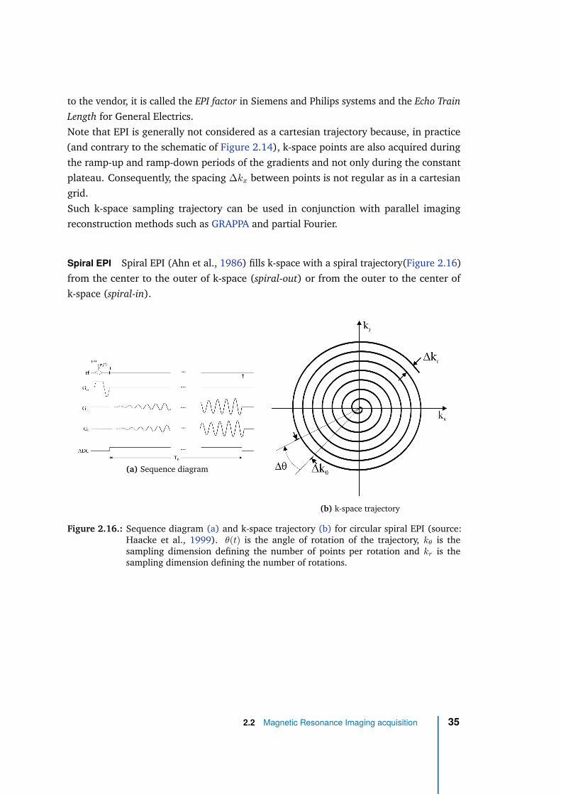
http://mriquestions.com/grappaarc.html

http://mriquestions.com/grappaarc.html

to the vendor, it is called the EPI factor in Siemens and Philips systems and the Echo Train

Length for General Electrics.

Note that EPI is generally not considered as a cartesian trajectory because, in practice

(and contrary to the schematic of Figure 2.14), k-space points are also acquired during

the ramp-up and ramp-down periods of the gradients and not only during the constant

plateau. Consequently, the spacing ∆kx between points is not regular as in a cartesian

grid.

Such k-space sampling trajectory can be used in conjunction with parallel imaging

reconstruction methods such as GRAPPA and partial Fourier.

Spiral EPI Spiral EPI (Ahn et al., 1986) fills k-space with a spiral trajectory(Figure 2.16)

from the center to the outer of k-space (spiral-out) or from the outer to the center of

k-space (spiral-in).

(a) Sequence diagram

(b) k-space trajectory

Figure 2.16.: Sequence diagram (a) and k-space trajectory (b) for circular spiral EPI (source:Haacke et al., 1999). θ(t) is the angle of rotation of the trajectory, kθ is thesampling dimension defining the number of points per rotation and kr is thesampling dimension defining the number of rotations.


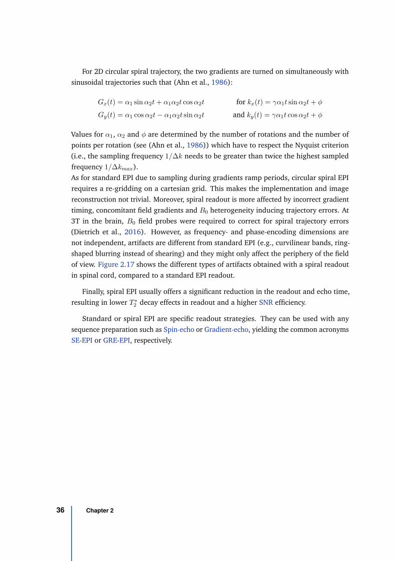
For 2D circular spiral trajectory, the two gradients are turned on simultaneously with

sinusoidal trajectories such that (Ahn et al., 1986):

Gx(t) = α1 sin α2t + α1α2t cos α2t for kx(t) = γα1t sin α2t + φ

Gy(t) = α1 cos α2t − α1α2t sin α2t and ky(t) = γα1t cos α2t + φ

Values for α1, α2 and φ are determined by the number of rotations and the number of

points per rotation (see (Ahn et al., 1986)) which have to respect the Nyquist criterion

(i.e., the sampling frequency 1/∆k needs to be greater than twice the highest sampled

frequency 1/∆kmax).

As for standard EPI due to sampling during gradients ramp periods, circular spiral EPI

requires a re-gridding on a cartesian grid. This makes the implementation and image

reconstruction not trivial. Moreover, spiral readout is more affected by incorrect gradient

timing, concomitant field gradients and B0 heterogeneity inducing trajectory errors. At

3T in the brain, B0 field probes were required to correct for spiral trajectory errors

(Dietrich et al., 2016). However, as frequency- and phase-encoding dimensions are

not independent, artifacts are different from standard EPI (e.g., curvilinear bands, ring-

shaped blurring instead of shearing) and they might only affect the periphery of the field

of view. Figure 2.17 shows the different types of artifacts obtained with a spiral readout

in spinal cord, compared to a standard EPI readout.

Finally, spiral EPI usually offers a significant reduction in the readout and echo time,

resulting in lower T ∗

2 decay effects in readout and a higher SNR efficiency.

Standard or spiral EPI are specific readout strategies. They can be used with any

sequence preparation such as Spin-echo or Gradient-echo, yielding the common acronyms

SE-EPI or GRE-EPI, respectively.

36 Chapter 2

(a) GRE sequence with circular spiral readout (b) GRE sequence with standard EPI readout

Figure 2.17.: Differences in the type of artifacts obtained in spinal cord with a Gradient-echo(GRE) sequence and spiral EPI (FOV=95×95mm2, matrix=128×128, TE=1.7ms)(a) or standard EPI readout (FOV=132×131mm2, matrix=178×176, TE=21.8ms)(a). Ring-shaped blurring can be observed with spiral EPI whereas the main artifactswith standard EPI are distortions in the phase-encoding direction (horizontal here).Those are images from exploratory non-optimized data acquired at the CRMBM.

2.3 Ultrahigh field MRI

In the context of clinical MRI, Ultrahigh Field (UHF) MRI refers to 7T MRI, while

high field MRI would refer to 3T MRI and low field MRI would describe field strength

of 1.5T and lower. The first 7T human MRI scanner appeared in the 2000s. Since

then, a hundred of them has been installed worldwide. The highest operational MRI

field strengths for human today (2020) are 9.4 T (five operational scanners across the

world) and 10.5 T (CMRR, University of Minnesota, Minneapolis). The Iseult project is

an ongoing French-German project aiming to build and use a human MRI scanner with

field strength 11.7 T in Paris-Saclay (Neurospin, CEA), by the 2021 horizon.

Up to now, clinical field strengths in use are 1.5 T and 3 T MRI. However, since 2017,

Siemens 7 T MRI (Magnetom Terra) has been approved for clinical use in Europe (Staff

News Brief, 2017) and the United-States (United States Food and Drug Administration,

2017). Even though it mostly remains at the stage of clinical research, new 7T installations

have skyrocketed across the world since then, making 7T MRI slowly but surely coming

to clinical routine.

2.3 Ultrahigh field MRI 37

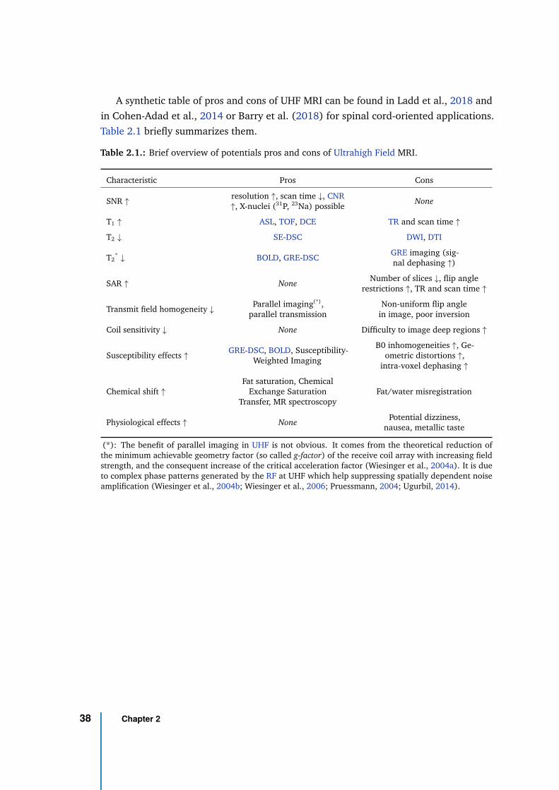
A synthetic table of pros and cons of UHF MRI can be found in Ladd et al., 2018 and

in Cohen-Adad et al., 2014 or Barry et al. (2018) for spinal cord-oriented applications.

Table 2.1 briefly summarizes them.

Table 2.1.: Brief overview of potentials pros and cons of Ultrahigh Field MRI.

Characteristic Pros Cons

SNR ↑resolution ↑, scan time ↓, CNR↑, X-nuclei (31P, 23Na) possible

None

T1 ↑ ASL, TOF, DCE TR and scan time ↑

T2 ↓ SE-DSC DWI, DTI

T2* ↓ BOLD, GRE-DSC

GRE imaging (sig-nal dephasing ↑)

SAR ↑ NoneNumber of slices ↓, flip angle

restrictions ↑, TR and scan time ↑

Transmit field homogeneity ↓Parallel imaging(*),

parallel transmissionNon-uniform flip angle

in image, poor inversion

Coil sensitivity ↓ None Difficulty to image deep regions ↑

Susceptibility effects ↑GRE-DSC, BOLD, Susceptibility-

Weighted Imaging

B0 inhomogeneities ↑, Ge-ometric distortions ↑,

intra-voxel dephasing ↑

Chemical shift ↑

Fat saturation, ChemicalExchange Saturation

Transfer, MR spectroscopyFat/water misregistration

Physiological effects ↑ NonePotential dizziness,

nausea, metallic taste

(*): The benefit of parallel imaging in UHF is not obvious. It comes from the theoretical reduction ofthe minimum achievable geometry factor (so called g-factor) of the receive coil array with increasing fieldstrength, and the consequent increase of the critical acceleration factor (Wiesinger et al., 2004a). It is dueto complex phase patterns generated by the RF at UHF which help suppressing spatially dependent noiseamplification (Wiesinger et al., 2004b; Wiesinger et al., 2006; Pruessmann, 2004; Ugurbil, 2014).

38 Chapter 2

2.3.1 Advantages of UHF MRI

Signal-to-Noise Ratio (SNR)

SNR dependency on field strength According to Equation (2.8) introduced in Sec-

tion 2.2.1, the NMR signal is detected by the electro-magnetic field emf induced by

the transverse magnetization Mxy precession in the coil after excitation by an RF pulse:

emf(t) = − d

dt

∫

sample

~M(~r, t) ~B−

1 (~r)d3r

where ~M is the net magnetization and ~B−

1 is the "receive" field of the detection coil

(magnetic field per unit current that would be produced by the detection coil).

Assuming an homogeneous sample and static field, with perfect and homogeneous RF

excitation, and ignoring the relaxation effects and the electronic amplification factors,

the signal amplitude expression can be simplified to:

|S| = ω0M0| ~B−

1 |xyVsample

with Vsample the volume of the sample and | ~B−

1 |xy =√

B−

1,x2

+ B−

1,y2 is the norm of ~B−

1

in the transverse plane. Signal amplitude is therefore proportional to B02.

Now, the noise (i.e., the perturbations coming from the system, the electronic compo-

nents or the sample) in NMR, is directly related to the effective resistance Reff "seen" by

the signal-receiving electronics. This resistance is the sum of the resistance of the sample,

the coil and the electronics. In particular, Hoult et al. (1979) studied the dieletric and

inductive losses in the human body. At low frequencies, the coil and electronics resistance

dominate whereas at high frequencies (B0 ≥ 0.5 T), the sample resistance dominates and

is proportional to ω02.

According to the Nyquist-Johnson theorem (Nyquist, 1928; Johnson, 1928), the vari-

ance of the fluctuating noise voltage σnoise is proportional to 4kT · Reff · BW with

BW the bandwidth of the reception coil, which is determined in NMR by the cutoff

frequency of the anti-aliasing low pass filter. Consequently, the Signal-to-Noise Ratio

(SNR)= S/σnoise = S/σthermal is proportional to B0 such that:

SNR ∝ B20√

B20

= B0 (2.21)


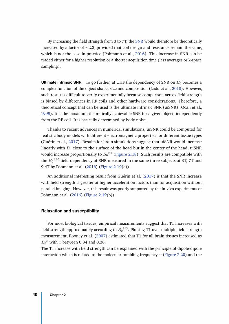
By increasing the field strength from 3 to 7T, the SNR would therefore be theoretically

increased by a factor of ∼2.3, provided that coil design and resistance remain the same,

which is not the case in practice (Pohmann et al., 2016). This increase in SNR can be

traded either for a higher resolution or a shorter acquisition time (less averages or k-space

sampling).

Ultimate intrinsic SNR To go further, at UHF the dependency of SNR on B0 becomes a

complex function of the object shape, size and composition (Ladd et al., 2018). However,

such result is difficult to verify experimentally because comparison across field strength

is biased by differences in RF coils and other hardware considerations. Therefore, a

theoretical concept that can be used is the ultimate intrinsic SNR (uiSNR) (Ocali et al.,

1998). It is the maximum theoretically achievable SNR for a given object, independently

from the RF coil. It is basically determined by body noise.

Thanks to recent advances in numerical simulations, uiSNR could be computed for

realistic body models with different electromagnetic properties for different tissue types

(Guérin et al., 2017). Results for brain simulations suggest that uiSNR would increase

linearly with B0 close to the surface of the head but in the center of the head, uiSNR

would increase proportionally to B02.1 (Figure 2.18). Such results are compatible with

the B01.65 field-dependency of SNR measured in the same three subjects at 3T, 7T and

9.4T by Pohmann et al. (2016) (Figure 2.19(a)).

An additional interesting result from Guérin et al. (2017) is that the SNR increase

with field strength is greater at higher acceleration factors than for acquisition without

parallel imaging. However, this result was poorly supported by the in-vivo experiments of

Pohmann et al. (2016) (Figure 2.19(b)).

Relaxation and susceptibility

For most biological tissues, empirical measurements suggest that T1 increases with

field strength approximately according to B01/3. Plotting T1 over multiple field strength

measurement, Rooney et al. (2007) estimated that T1 for all brain tissues increased as

B0x with x between 0.34 and 0.38.

The T1 increase with field strength can be explained with the principle of dipole-dipole

interaction which is related to the molecular tumbling frequency ω (Figure 2.20) and the

40 Chapter 2

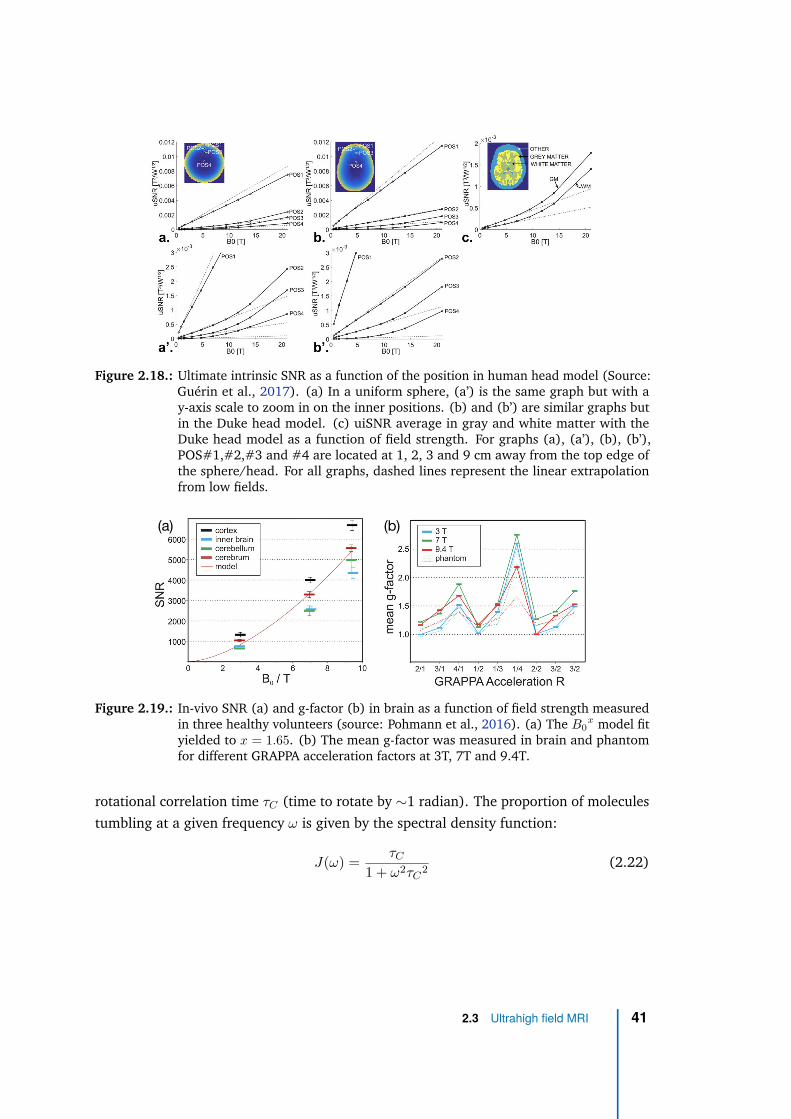
Figure 2.18.: Ultimate intrinsic SNR as a function of the position in human head model (Source:Guérin et al., 2017). (a) In a uniform sphere, (a’) is the same graph but with ay-axis scale to zoom in on the inner positions. (b) and (b’) are similar graphs butin the Duke head model. (c) uiSNR average in gray and white matter with theDuke head model as a function of field strength. For graphs (a), (a’), (b), (b’),POS#1,#2,#3 and #4 are located at 1, 2, 3 and 9 cm away from the top edge ofthe sphere/head. For all graphs, dashed lines represent the linear extrapolationfrom low fields.

(b)(a)

Figure 2.19.: In-vivo SNR (a) and g-factor (b) in brain as a function of field strength measuredin three healthy volunteers (source: Pohmann et al., 2016). (a) The B0

x model fityielded to x = 1.65. (b) The mean g-factor was measured in brain and phantomfor different GRAPPA acceleration factors at 3T, 7T and 9.4T.

rotational correlation time τC (time to rotate by ∼1 radian). The proportion of molecules

tumbling at a given frequency ω is given by the spectral density function:

J(ω) =τC

1 + ω2τC2

(2.22)


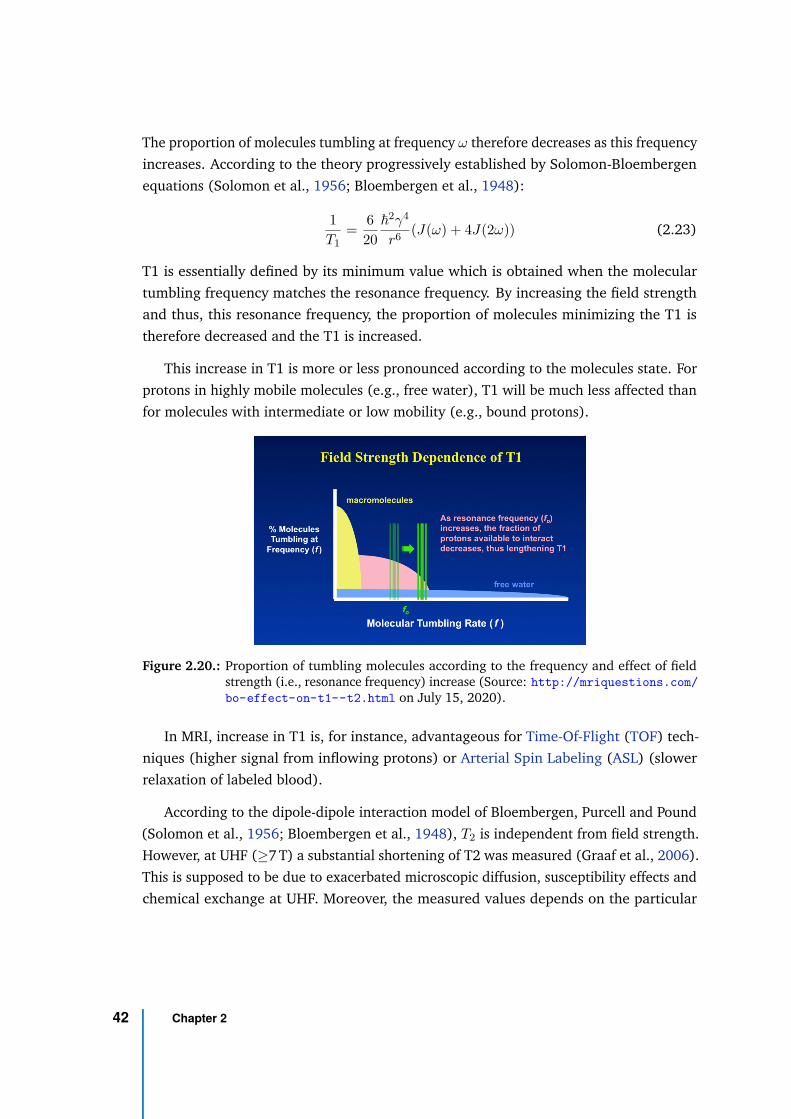
The proportion of molecules tumbling at frequency ω therefore decreases as this frequency

increases. According to the theory progressively established by Solomon-Bloembergen

equations (Solomon et al., 1956; Bloembergen et al., 1948):

1

T1=

6

20

~2γ4

r6(J(ω) + 4J(2ω)) (2.23)

T1 is essentially defined by its minimum value which is obtained when the molecular

tumbling frequency matches the resonance frequency. By increasing the field strength

and thus, this resonance frequency, the proportion of molecules minimizing the T1 is

therefore decreased and the T1 is increased.

This increase in T1 is more or less pronounced according to the molecules state. For

protons in highly mobile molecules (e.g., free water), T1 will be much less affected than

for molecules with intermediate or low mobility (e.g., bound protons).

Figure 2.20.: Proportion of tumbling molecules according to the frequency and effect of fieldstrength (i.e., resonance frequency) increase (Source: http://mriquestions.com/

bo-effect-on-t1--t2.html on July 15, 2020).

In MRI, increase in T1 is, for instance, advantageous for Time-Of-Flight (TOF) tech-

niques (higher signal from inflowing protons) or Arterial Spin Labeling (ASL) (slower

relaxation of labeled blood).

According to the dipole-dipole interaction model of Bloembergen, Purcell and Pound

(Solomon et al., 1956; Bloembergen et al., 1948), T2 is independent from field strength.

However, at UHF (≥7 T) a substantial shortening of T2 was measured (Graaf et al., 2006).

This is supposed to be due to exacerbated microscopic diffusion, susceptibility effects and

chemical exchange at UHF. Moreover, the measured values depends on the particular

42 Chapter 2

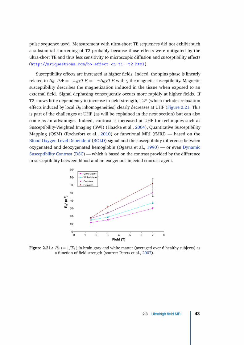
http://mriquestions.com/bo-effect-on-t1--t2.html


pulse sequence used. Measurement with ultra-short TE sequences did not exhibit such

a substantial shortening of T2 probably because those effects were mitigated by the

ultra-short TE and thus less sensitivity to microscopic diffusion and susceptibility effects

(http://mriquestions.com/bo-effect-on-t1--t2.html).

Susceptibility effects are increased at higher fields. Indeed, the spins phase is linearly

related to B0: ∆Φ = −ω0χTE = −γB0χTE with χ the magnetic susceptibility. Magnetic

susceptibility describes the magnetization induced in the tissue when exposed to an

external field. Signal dephasing consequently occurs more rapidly at higher fields. If

T2 shows little dependency to increase in field strength, T2* (which includes relaxation

effects induced by local B0 inhomogeneities) clearly decreases at UHF (Figure 2.21. This

is part of the challenges at UHF (as will be explained in the next section) but can also

come as an advantage. Indeed, contrast is increased at UHF for techniques such as

Susceptibility-Weighted Imaging (SWI) (Haacke et al., 2004), Quantitative Susceptibility

Mapping (QSM) (Rochefort et al., 2010) or functional MRI (fMRI) — based on the

Blood Oxygen Level Dependent (BOLD) signal and the susceptibility difference between

oxygenated and deoxygenated hemoglobin (Ogawa et al., 1990) — or even Dynamic

Susceptibility Contrast (DSC) — which is based on the contrast provided by the difference

in susceptibility between blood and an exogenous injected contrast agent.

Figure 2.21.: R∗

2(= 1/T ∗

2) in brain gray and white matter (averaged over 6 healthy subjects) as

a function of field strength (source: Peters et al., 2007).



Chemical shift

Chemical shift refers to the little differences in Larmor frequencies of protons induced

by the different molecular environments. The most common example in MRI is the

chemical shift between fat protons and water protons. Fat protons are covered by electron

clouds coming from the long-chain triglycerides they are nestled in and which act as

a shield to the external magnetic field. Water protons are less shielded because of the

highly electronegative oxygen atom pulling away the electrons. Fat protons therefore

have a lower Larmor frequency by 3.4 parts per million (ppm) than water protons. This

can lead to chemical shift artifact caused by an incorrect position of the fat signal with

respect to water signal in the frequency-encoding direction (or phase-encoding direction

in EPI). Increasing B0 thus linearly increases the chemical shift.

In some applications however, the chemical shift is an advantage as source of contrast.

Indeed, the chemical shift between metabolites (e.g., to differentiate glutamate (Glu)

and glutamine (Gln)) is the fundamental of Magnetic Resonance Spectroscopy (MRS).

UHF therefore increases the spectral resolution, helping the separation of the different

metabolites. Chemical Exchange Saturation Transfer (CEST) (Ward et al., 2000) is

another technique benefiting from the increased chemical shift at UHF, as separation of

CEST peaks between diluted molecules is made easier.

The increased chemical shift between fat and water protons at UHF is also an advan-

tage for fat saturation techniques prior to imaging.

2.3.2 Disadvantages and challenges of UHF MRI

Static field inhomogeneities

B0 field inhomogeneities originate from two sources. The first one is related to

hardware. Imperfections of the static field produced by the magnet are more important

at UHF as it becomes more and more challenging to build magnets with uniform static

field when the field strength increases, as for wide bores and short magnets. As a result,

7T magnets show a static field homogeneous over a reduced volume around the isocenter

compared to 3T, and are longer with narrower bores (e.g., 270 cm×60 cm for Siemens

Magnetom Terra 7T versus 173 cm×70 cm Siemens Magnetom Skyra 3T).

44 Chapter 2

The second source of inhomogeneity is the object or subject introduced in the magnet.

The inhomogeneities in magnetic susceptibility related to tissue proportionally convert

into field inhomogeneities, which scale with B0. Susceptibility inhomogeneities can be

static (e.g., between air and tissue) or dynamic (e.g., fluctuating air volume in lungs with

breathing).

In spinal cord, static inhomogeneities are high because of the different tissue types

in immediate vicinity (CSF, vertebrae bone, intervertebral disks, soft tissue) and the

longitudinal tubular shape of the cord. But in addition, the close proximity of the lungs

and trachea, filled of air with a volume that fluctuates with breathing, is a source of

dynamic inhomogeneities (Verma et al., 2014; Vannesjo et al., 2018). CSF pulses with

heartbeat during the acquisition bring additional dynamic field inhomogeneities (Hu

et al., 1995).

Even at 3T, and even at the highest cervical levels, breathing-induced B0 variations were

measured, with a great variability across subjects (Figure 2.22). Such variations are

increased at 7T up to 95 Hz in average (Vannesjo et al., 2018) or higher (Pennell et al.,

2014), compared to 75 Hz at 3T. In comparison, breathing-induced B0 fluctuations in

brain at 7T were estimaged at 7 Hz during deep breathing (Duerst et al., 2016). According

to Vannesjo et al. (2018), the B0 shift between inspiration and expiration can go up to

more than 200 Hz.

Those increased B0 inhomogeneities at 7T are particularly detrimental to sequences

such as single-shot EPI, which has a very low BW in the phase-encoding direction,

resulting in large geometric distortions. If identical gradient strength is used, a BW 2.3

times higher than what is used at 3T would be necessary to obtain the same level of

distortions at 7T. However, this would considerably lower the SNR. Fortunately, new 7T

systems include gradient coils capable of higher gradient strengths compared to 3T.

Field inhomogeneities are local strong gradients, of the same order as the maximum

gradient strength of current 7T gradient coils. By way of example, the susceptibility

difference between air and soft-tissue is 9.4 ppm, corresponding to a frequency shift

of 2.8 kHz whereas the maximum gradient strength of 7T systems such as the Siemens

Terra scanner is 80 mT/m, which is equivalent to a frequency shift of 3.4 kHz/mm. B0

shimming is thus used to correct for field inhomogeneity using dedicated shim coils

inserted in the magnet bore. Standard B0 shimming procedures measure frequency

shifts by means of a B0 field map (or a set of projections in different orientations) and

then apply an algorithm in order to determine the external magnetic field to apply (and

corresponding currents for the shim coil) to counteract those local inhomogeneities. As


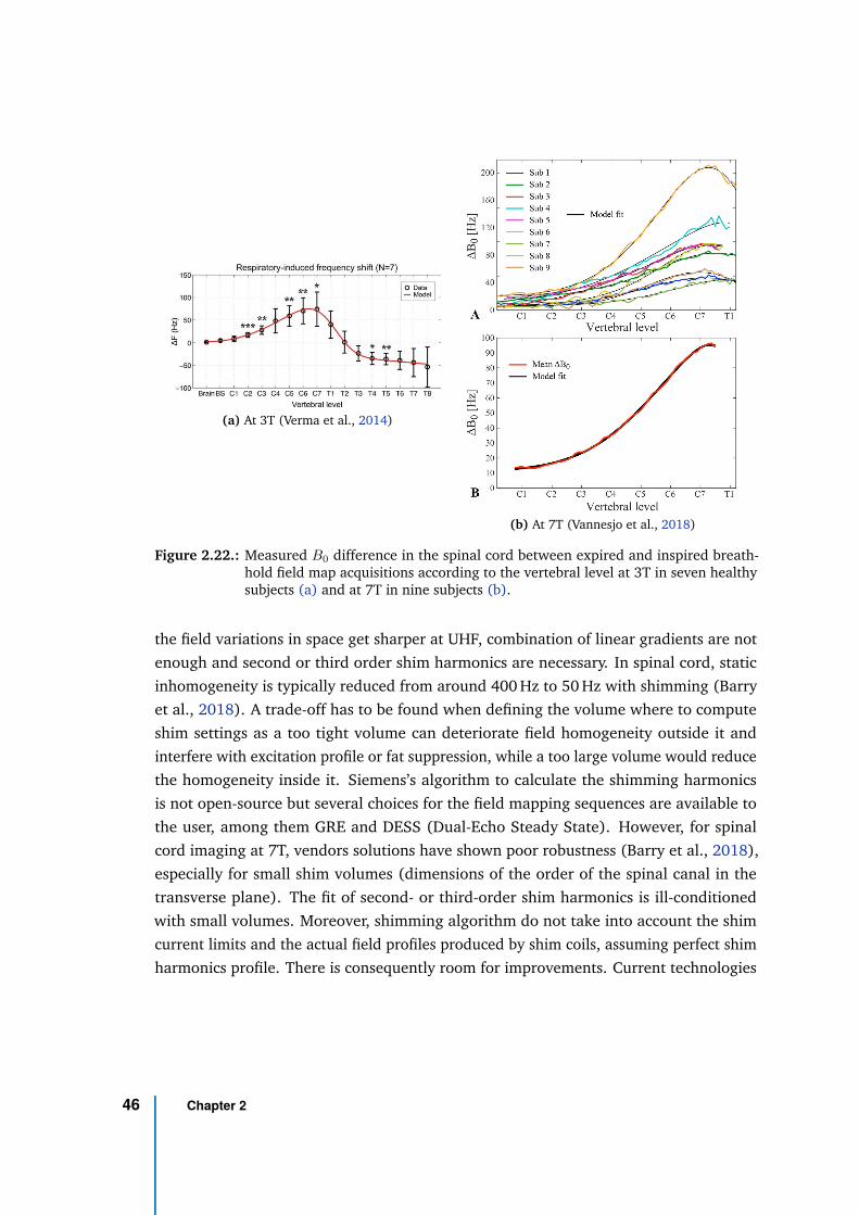
(a) At 3T (Verma et al., 2014)

(b) At 7T (Vannesjo et al., 2018)

Figure 2.22.: Measured B0 difference in the spinal cord between expired and inspired breath-hold field map acquisitions according to the vertebral level at 3T in seven healthysubjects (a) and at 7T in nine subjects (b).

the field variations in space get sharper at UHF, combination of linear gradients are not

enough and second or third order shim harmonics are necessary. In spinal cord, static

inhomogeneity is typically reduced from around 400 Hz to 50 Hz with shimming (Barry

et al., 2018). A trade-off has to be found when defining the volume where to compute

shim settings as a too tight volume can deteriorate field homogeneity outside it and

interfere with excitation profile or fat suppression, while a too large volume would reduce

the homogeneity inside it. Siemens’s algorithm to calculate the shimming harmonics

is not open-source but several choices for the field mapping sequences are available to

the user, among them GRE and DESS (Dual-Echo Steady State). However, for spinal

cord imaging at 7T, vendors solutions have shown poor robustness (Barry et al., 2018),

especially for small shim volumes (dimensions of the order of the spinal canal in the

transverse plane). The fit of second- or third-order shim harmonics is ill-conditioned

with small volumes. Moreover, shimming algorithm do not take into account the shim

current limits and the actual field profiles produced by shim coils, assuming perfect shim

harmonics profile. There is consequently room for improvements. Current technologies

46 Chapter 2

consider arrays of small shim coils placed close to the subject, which have demonstrated

improved shimming performance at 7T in the brain (Juchem et al., 2011)). Such set-up

was also adopted for spinal cord coil design (Topfer et al., 2016) and is very promising.

Those systems however fail to correct for dynamic field inhomogeneity or drastic

field variations along the inferior-superior direction as occur in spinal cord imaging at

7T when dealing with large FOV (e.g., from C1 to C7). Several strategies have been

proposed to address these problems. The first approach is to correct the inhomogeneity

during acquisition using dynamic shimming system in order to adjust the corrective field

(shimming settings) for each slice (slice-wise shimming) (Juchem et al., 2010; Sengupta

et al., 2011). Even the dynamic update of first-order shim along inferior-superior axis

has shown significant improvement for multi-slice spinal cord acquisitions (Finsterbusch

et al., 2013). To correct for time-fluctuating inhomogeneities like breathing-induced

variations, an adaptation of shim currents in real-time is necessary (real-time shimming).

However, real-time control of shim settings requires specific hardware (Topfer et al.,

2018) or modifications of current hardware (Gelderen et al., 2007). The second approach

is to correct the data retrospectively during reconstruction. FID navigators are used to

monitor the spatiotemporal B0 field changes in real time and then incorporate them

into a restrospective iterative reconstruction to improve 2D GRE images of the brain

(Wallace et al., 2019). In spinal cord, Vannesjo et al. (2019) proposed a method to

correct the acquired k-space data by the phase offset induced by breathing. This phase

offset was deduced from the respiratory belt signal and reference field maps acquired

beforehand and used to calibrate the relation between respiratory belt signal and B0 offset

individually for each slice and each subject. Finally, the third approach is to use pads

filled with specific materials matching the susceptibility of human tissue and to position

them in the vicinity of the subject (passive B0 shimming), which would mostly mitigate

inhomogeneities close to the shoulder but would not help with dynamic variations. Lee

et al. (2015) demonstrated an improved field homogeneity at 3T in the spinal cord with

pyrolytic graphite foam placed around the neck of the subject. A fourth option would be

to synchronize B0 shimming and EPI acquisitions with respiration.

Transmit field inhomogeneities and energy deposition

As the transmit field frequency increases with static field strength, the wavelength

of excitation pulses is reduced and becomes comparable to the human body and head

dimensions. At 7T the electromagnetic wavelength is close to the human body and head


dimensions (λRF ≈ 13.4 cm in brain tissue at 300 MHz) (Collins et al., 2011). Reflection

and scattering effects of the electromagnetic wave entering the body are thus increased

and lead to higher transmit field inhomogeneity with substantial local voids. The energy

of the electromagnetic wave is also increased (E = hf0). In addition, while the magnetic

component of the transmit RF field interact with the spin to flip the magnetization, the

spatially varying non-conservative electric component ~E that accompanies it displaces

charges in the tissue, creating electric currents, which convert into heating and energy

deposition with the natural resistive losses of the human tissue. The Specific Absorption

Rate (SAR) quantifies the energy deposition in the tissue according to:

SAR =σ| ~E(~r)|

2ρ

with σ the conductivity and ρ the mass density of the tissue. According to Faraday’s law,

the electric component is related to the temporal derivative of the magnetic component

by:

∇ × ~E = −∂ ~B

∂t

As the frequency of the RF pulse is increased at higher field, the magnetic component

changes faster with time, hence the increased electric field and SAR at higher field.

For field strengths up to 3T, SAR approximately increases as B02. At UHF, the electric

field distribution becomes more inhomogeneous with so-called hot spots that can induce

local SAR peaks compared to surrounding tissue. The local-to-global SAR ratio may be

substantially increased. Therefore, the extrapolation of SAR distribution at UHF is non-

trivial and may deviate from the quadratic increase with field strength. Although active

research is looking at reliable solutions to measure temperature and SAR with MRI (MRI

thermometry), since SAR is caused by the electric field and not the magnetic component,

measurements are mainly performed with numerical eletromagnetic simulations with

virtual coil and human body model.

In summary, not only does the RF power necessary to tilt the magnetization by the desired

flip angle increase at UHF, leading to SAR restrictions, but also the SAR distribution

gets more heterogeneous with local heating spots that can potentially cause tissue

damage. To ensure patients’ safety, the maximum SAR exposure is limited by regulatory

authorities (International Electrotechnical Commission, 2015; United States Food and

Drug Administration, 2014). In European Union for example, the global SAR is limited to

an average value of 3.2 W/kg by 6-minute time periods. The local SAR for each 10g of

tissue is limited to a maximum of 10 W/kg, and 30 W/kg over any 10-second period.

48 Chapter 2

Those limitations are the same regardless of the field strength but are more restricting

at UHF for the reasons aforementioned. In practice, workarounds are to lengthen RF

pulses, prescribe smaller flip angle, reduce the number of slices or lengthen repetition

time at the cost of the scan duration. Nevertheless, those workarounds are quickly limited.

To fully unlock the potential of UHF MRI, the independent usage of different transmit

coil channels emerged as a solution (Katscher et al., 2006; Zhu, 2004; Katscher et al.,

2003). Thanks to individual design of the pulse profiles of each transmission channel of

the coil, parallel transmission (pTx) techniques take advantage of the higher degrees of

freedom to improve the spatial homogeneity of the resultant transmit field in the region

of interest and to reduce SAR.

Furthermore, as proposed for static field heterogeneity, transmit field homogeneity

and efficiency at UHF can be improved with dieletric pads filled with high-permittivity

materials (Teeuwisse et al., 2012). Those pads are positioned between the coil and the

subject. However, as with pTx, the transmit field distribution of the coil is modified and

therefore requires a validation (e.g., using electromagnetic numerical simulations) to

ensure that no local SAR hot spots are created that could induce tissue damage.

Physiological effects of UHF

Physiological effects on patients pointed out during the development stage of 7T MRI

are of critical importance for the clinical acceptance of UHF. Beyond the local SAR hotspots

that are more likely at high field strength, dizziness, nausea, vertigo, magnetophosphenes

or metallic taste have been reported (Heilmaier et al., 2011). Disturbance of the vestibular

system leading to an incongruence between sensory, proprioceptive and visual information

received by the brain are suspected to be responsible for dizziness, nausea and vertigo

(Mian et al., 2016; Thormann et al., 2013). An increased blood pressure due to increased

static field strength was also investigated. Magnetohydrodynamic models have estimated

an increased pressure by less than 0.2% for a 10T field change (Keltner et al., 1990) and

experimental measurements in human and large animals did not find significant effects

(Atkinson et al., 2007).

If the aforementioned effects are categorized as transitory effects, permanent effect

with negative long-term health consequences of UHF, and more generally of MRI, have

been investigated. The main concern regards DNA damage and especially double-strand

breaks (DSB) which can lead to cell death or degeneration and cancerogenesis. Such

damage would mainly result from the interaction of high-energy photons with H2O


generating free radicals (e.g., OH-). Two out of seven studies reported increase in

staining for DSB in blood before and after MRI exposure. However, the studies with the

largest sample size, highest field strength (up to 7T) and including frequently exposed

subjects did not find any significant effect, concluding that DNA damage induced by MRI

up to 7T is not a relevant concern (Brand et al., 2015; Lancellotti et al., 2015; Reddig

et al., 2015).

Either it exist or not, these effects might be close to the limit of detection of the

current techniques or similar to the variations with everyday life activities. The RF

quantum energy (10−6 eV at 7T) is much smaller than the Boltzmann thermal energy at

the human body temperature (about 27 × 10−3 eV) or than the ionization or excitation

energies in molecules (about 1 eV). Thus, potential effects during medical MR exams in

clinics (clinical exposure) should not be reconsidered. Concerns are for research practice

(research exposure) where subject are exposed without direct benefit for them. Regarding

the exposure of workers to higher magnetic fields (occupational exposure), activities

which require approaching the bore or reaching into it should be monitored as limits

have been defined by the European Union Electromagnetic Field Directive (2 T for normal

working conditions, 8 T for localized exposure of the limbs, 8T for controlled working

conditions) (European Parliament and Council, 2013).

2.3.3 UHF MRI in spinal cord

The main centers deeply involved in 7T spinal cord imaging across the world are

currently Vanderbilt University Institute of Imaging Science (Nashville, USA), Oxford

Centre for Functional MRI of the Brain (Oxford, UK), Athinoula A. Martinos Center for

Biomedical Imaging (MGH, Charlestown, USA), Icahn School of Medicine at Mount

Sinai (New York, USA) and Center for Magnetic Resonance in Biology and Medicine (Aix-

Marseille University, Marseille, France), recently joined by Montreal Neurological Institute

(Montreal, Canada) and the Balgrist Spinal Cord Injury Center (Zurich, Switzerland).

7T spine coil arrays

Several designs have been proposed for spinal cord MRI coils at 7T. A comprehensive

review is available in Barry et al., 2018 (see Figure 2).

50 Chapter 2

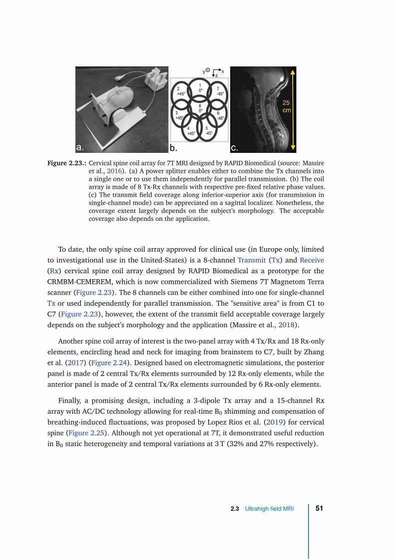
Figure 2.23.: Cervical spine coil array for 7T MRI designed by RAPID Biomedical (source: Massireet al., 2016). (a) A power splitter enables either to combine the Tx channels intoa single one or to use them independently for parallel transmission. (b) The coilarray is made of 8 Tx-Rx channels with respective pre-fixed relative phase values.(c) The transmit field coverage along inferior-superior axis (for transmission insingle-channel mode) can be appreciated on a sagittal localizer. Nonetheless, thecoverage extent largely depends on the subject’s morphology. The acceptablecoverage also depends on the application.

To date, the only spine coil array approved for clinical use (in Europe only, limited

to investigational use in the United-States) is a 8-channel Transmit (Tx) and Receive

(Rx) cervical spine coil array designed by RAPID Biomedical as a prototype for the

CRMBM-CEMEREM, which is now commercialized with Siemens 7T Magnetom Terra

scanner (Figure 2.23). The 8 channels can be either combined into one for single-channel

Tx or used independently for parallel transmission. The "sensitive area" is from C1 to

C7 (Figure 2.23), however, the extent of the transmit field acceptable coverage largely

depends on the subject’s morphology and the application (Massire et al., 2018).

Another spine coil array of interest is the two-panel array with 4 Tx/Rx and 18 Rx-only

elements, encircling head and neck for imaging from brainstem to C7, built by Zhang

et al. (2017) (Figure 2.24). Designed based on electromagnetic simulations, the posterior

panel is made of 2 central Tx/Rx elements surrounded by 12 Rx-only elements, while the

anterior panel is made of 2 central Tx/Rx elements surrounded by 6 Rx-only elements.

Finally, a promising design, including a 3-dipole Tx array and a 15-channel Rx

array with AC/DC technology allowing for real-time B0 shimming and compensation of

breathing-induced fluctuations, was proposed by Lopez Rios et al. (2019) for cervical

spine (Figure 2.25). Although not yet operational at 7T, it demonstrated useful reduction

in B0 static heterogeneity and temporal variations at 3 T (32% and 27% respectively).


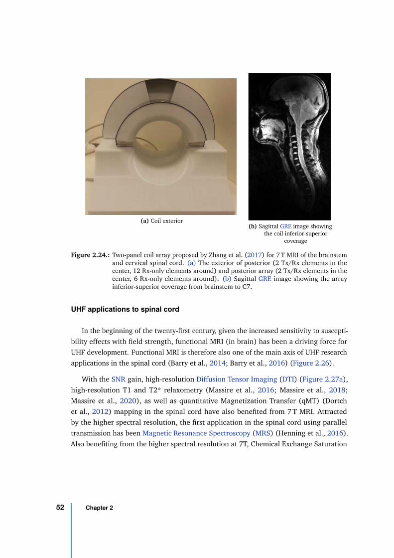
(a) Coil exterior(b) Sagittal GRE image showing

the coil inferior-superiorcoverage

Figure 2.24.: Two-panel coil array proposed by Zhang et al. (2017) for 7 T MRI of the brainstemand cervical spinal cord. (a) The exterior of posterior (2 Tx/Rx elements in thecenter, 12 Rx-only elements around) and posterior array (2 Tx/Rx elements in thecenter, 6 Rx-only elements around). (b) Sagittal GRE image showing the arrayinferior-superior coverage from brainstem to C7.

UHF applications to spinal cord

In the beginning of the twenty-first century, given the increased sensitivity to suscepti-

bility effects with field strength, functional MRI (in brain) has been a driving force for

UHF development. Functional MRI is therefore also one of the main axis of UHF research

applications in the spinal cord (Barry et al., 2014; Barry et al., 2016) (Figure 2.26).

With the SNR gain, high-resolution Diffusion Tensor Imaging (DTI) (Figure 2.27a),

high-resolution T1 and T2* relaxometry (Massire et al., 2016; Massire et al., 2018;

Massire et al., 2020), as well as quantitative Magnetization Transfer (qMT) (Dortch

et al., 2012) mapping in the spinal cord have also benefited from 7 T MRI. Attracted

by the higher spectral resolution, the first application in the spinal cord using parallel

transmission has been Magnetic Resonance Spectroscopy (MRS) (Henning et al., 2016).

Also benefiting from the higher spectral resolution at 7T, Chemical Exchange Saturation

52 Chapter 2

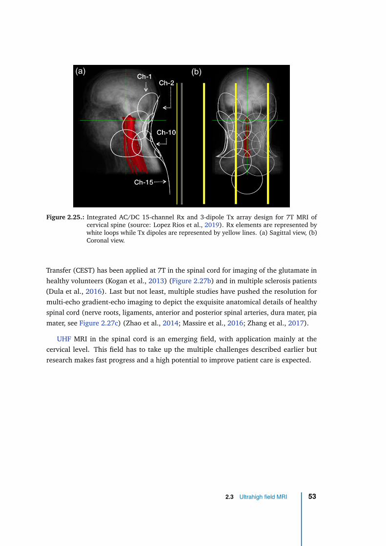
Figure 2.25.: Integrated AC/DC 15-channel Rx and 3-dipole Tx array design for 7T MRI ofcervical spine (source: Lopez Rios et al., 2019). Rx elements are represented bywhite loops while Tx dipoles are represented by yellow lines. (a) Sagittal view, (b)Coronal view.

Transfer (CEST) has been applied at 7T in the spinal cord for imaging of the glutamate in

healthy volunteers (Kogan et al., 2013) (Figure 2.27b) and in multiple sclerosis patients

(Dula et al., 2016). Last but not least, multiple studies have pushed the resolution for

multi-echo gradient-echo imaging to depict the exquisite anatomical details of healthy

spinal cord (nerve roots, ligaments, anterior and posterior spinal arteries, dura mater, pia

mater, see Figure 2.27c) (Zhao et al., 2014; Massire et al., 2016; Zhang et al., 2017).

UHF MRI in the spinal cord is an emerging field, with application mainly at the

cervical level. This field has to take up the multiple challenges described earlier but

research makes fast progress and a high potential to improve patient care is expected.


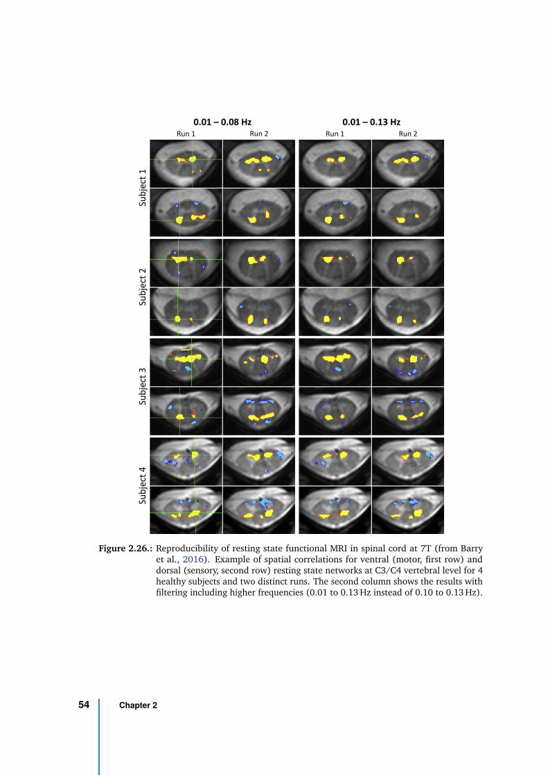
Figure 2.26.: Reproducibility of resting state functional MRI in spinal cord at 7T (from Barryet al., 2016). Example of spatial correlations for ventral (motor, first row) anddorsal (sensory, second row) resting state networks at C3/C4 vertebral level for 4healthy subjects and two distinct runs. The second column shows the results withfiltering including higher frequencies (0.01 to 0.13 Hz instead of 0.10 to 0.13 Hz).

54 Chapter 2

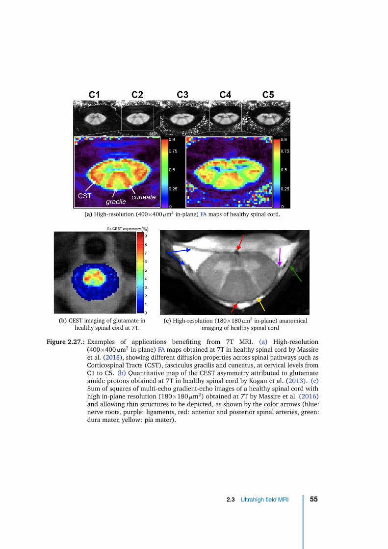
(a) High-resolution (400×400 µm2 in-plane) FA maps of healthy spinal cord.

(b) CEST imaging of glutamate inhealthy spinal cord at 7T.

(c) High-resolution (180×180 µm2 in-plane) anatomicalimaging of healthy spinal cord

Figure 2.27.: Examples of applications benefiting from 7T MRI. (a) High-resolution(400×400 µm2 in-plane) FA maps obtained at 7T in healthy spinal cord by Massireet al. (2018), showing different diffusion properties across spinal pathways such asCorticospinal Tracts (CST), fasciculus gracilis and cuneatus, at cervical levels fromC1 to C5. (b) Quantitative map of the CEST asymmetry attributed to glutamateamide protons obtained at 7T in healthy spinal cord by Kogan et al. (2013). (c)Sum of squares of multi-echo gradient-echo images of a healthy spinal cord withhigh in-plane resolution (180×180 µm2) obtained at 7T by Massire et al. (2016)and allowing thin structures to be depicted, as shown by the color arrows (blue:nerve roots, purple: ligaments, red: anterior and posterior spinal arteries, green:dura mater, yellow: pia mater).


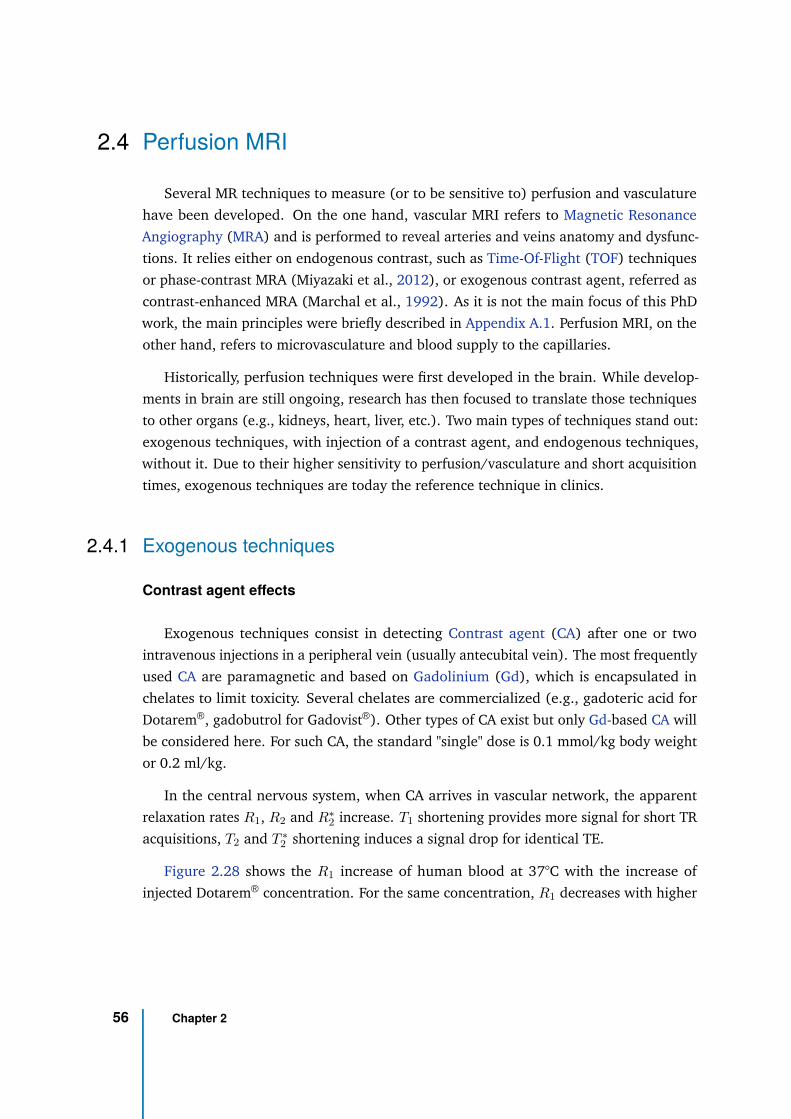
2.4 Perfusion MRI

Several MR techniques to measure (or to be sensitive to) perfusion and vasculature

have been developed. On the one hand, vascular MRI refers to Magnetic Resonance

Angiography (MRA) and is performed to reveal arteries and veins anatomy and dysfunc-

tions. It relies either on endogenous contrast, such as Time-Of-Flight (TOF) techniques

or phase-contrast MRA (Miyazaki et al., 2012), or exogenous contrast agent, referred as

contrast-enhanced MRA (Marchal et al., 1992). As it is not the main focus of this PhD

work, the main principles were briefly described in Appendix A.1. Perfusion MRI, on the

other hand, refers to microvasculature and blood supply to the capillaries.

Historically, perfusion techniques were first developed in the brain. While develop-

ments in brain are still ongoing, research has then focused to translate those techniques

to other organs (e.g., kidneys, heart, liver, etc.). Two main types of techniques stand out:

exogenous techniques, with injection of a contrast agent, and endogenous techniques,

without it. Due to their higher sensitivity to perfusion/vasculature and short acquisition

times, exogenous techniques are today the reference technique in clinics.

2.4.1 Exogenous techniques

Contrast agent effects

Exogenous techniques consist in detecting Contrast agent (CA) after one or two

intravenous injections in a peripheral vein (usually antecubital vein). The most frequently

used CA are paramagnetic and based on Gadolinium (Gd), which is encapsulated in

chelates to limit toxicity. Several chelates are commercialized (e.g., gadoteric acid for

Dotarem®, gadobutrol for Gadovist®). Other types of CA exist but only Gd-based CA will

be considered here. For such CA, the standard "single" dose is 0.1 mmol/kg body weight

or 0.2 ml/kg.

In the central nervous system, when CA arrives in vascular network, the apparent

relaxation rates R1, R2 and R∗

2 increase. T1 shortening provides more signal for short TR

acquisitions, T2 and T ∗

2 shortening induces a signal drop for identical TE.

Figure 2.28 shows the R1 increase of human blood at 37°C with the increase of

injected Dotarem® concentration. For the same concentration, R1 decreases with higher

56 Chapter 2

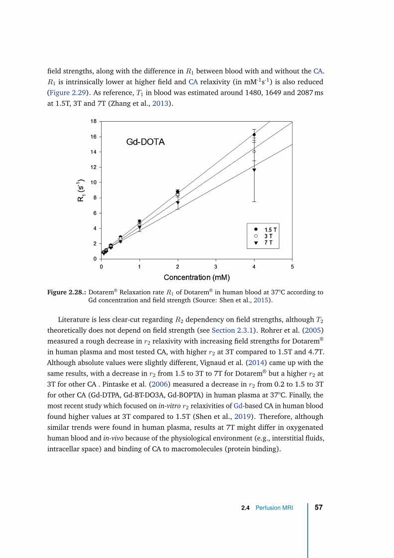
field strengths, along with the difference in R1 between blood with and without the CA.

R1 is intrinsically lower at higher field and CA relaxivity (in mM-1s-1) is also reduced

(Figure 2.29). As reference, T1 in blood was estimated around 1480, 1649 and 2087 ms

at 1.5T, 3T and 7T (Zhang et al., 2013).

Figure 2.28.: Dotarem® Relaxation rate R1 of Dotarem® in human blood at 37°C according toGd concentration and field strength (Source: Shen et al., 2015).

Literature is less clear-cut regarding R2 dependency on field strengths, although T2

theoretically does not depend on field strength (see Section 2.3.1). Rohrer et al. (2005)

measured a rough decrease in r2 relaxivity with increasing field strengths for Dotarem®

in human plasma and most tested CA, with higher r2 at 3T compared to 1.5T and 4.7T.

Although absolute values were slightly different, Vignaud et al. (2014) came up with the

same results, with a decrease in r2 from 1.5 to 3T to 7T for Dotarem® but a higher r2 at

3T for other CA . Pintaske et al. (2006) measured a decrease in r2 from 0.2 to 1.5 to 3T

for other CA (Gd-DTPA, Gd-BT-DO3A, Gd-BOPTA) in human plasma at 37°C. Finally, the

most recent study which focused on in-vitro r2 relaxivities of Gd-based CA in human blood

found higher values at 3T compared to 1.5T (Shen et al., 2019). Therefore, although

similar trends were found in human plasma, results at 7T might differ in oxygenated

human blood and in-vivo because of the physiological environment (e.g., interstitial fluids,

intracellar space) and binding of CA to macromolecules (protein binding).

2.4 Perfusion MRI 57

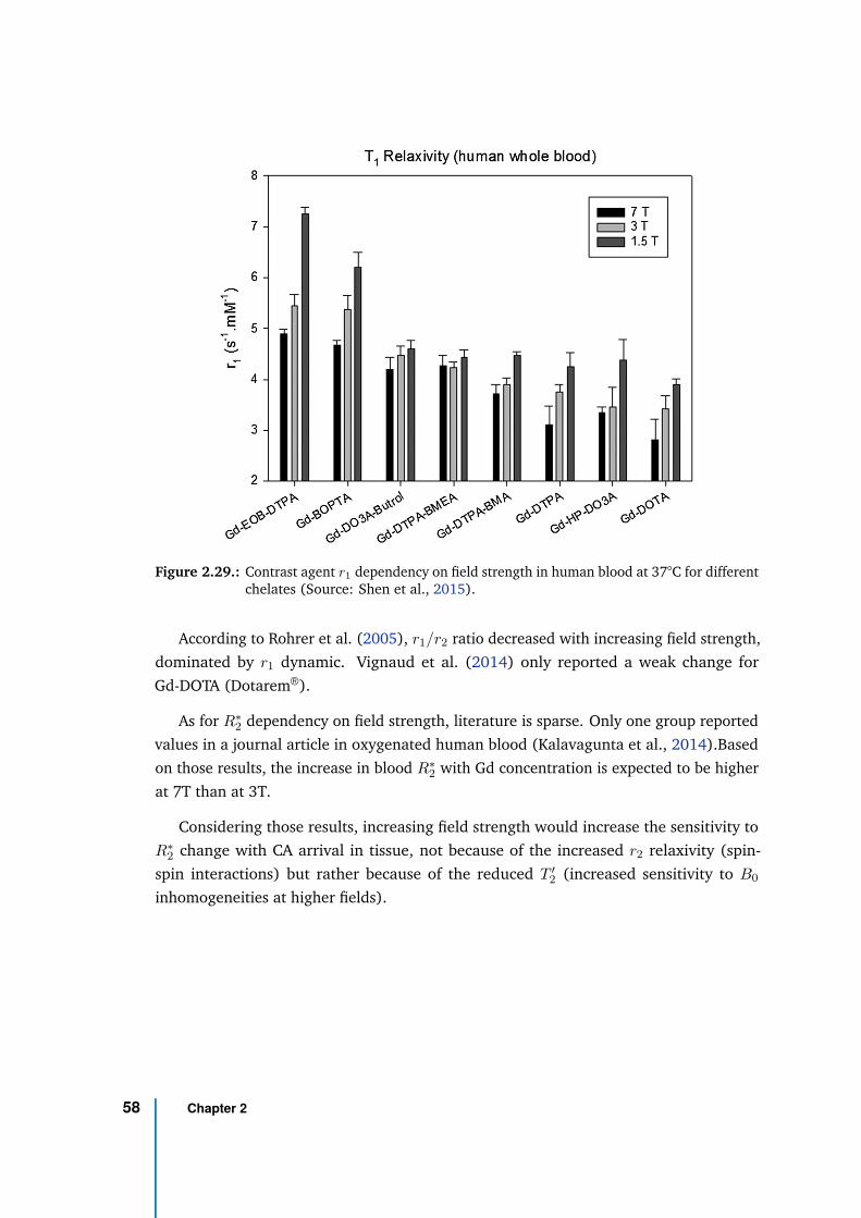
Figure 2.29.: Contrast agent r1 dependency on field strength in human blood at 37°C for differentchelates (Source: Shen et al., 2015).

According to Rohrer et al. (2005), r1/r2 ratio decreased with increasing field strength,

dominated by r1 dynamic. Vignaud et al. (2014) only reported a weak change for

Gd-DOTA (Dotarem®).

As for R∗

2 dependency on field strength, literature is sparse. Only one group reported

values in a journal article in oxygenated human blood (Kalavagunta et al., 2014).Based

on those results, the increase in blood R∗

2 with Gd concentration is expected to be higher

at 7T than at 3T.

Considering those results, increasing field strength would increase the sensitivity to

R∗

2 change with CA arrival in tissue, not because of the increased r2 relaxivity (spin-

spin interactions) but rather because of the reduced T ′

2 (increased sensitivity to B0

inhomogeneities at higher fields).

58 Chapter 2

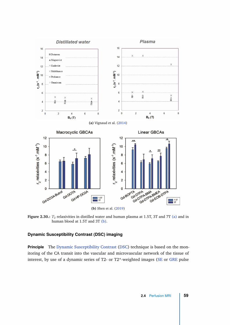
(a) Vignaud et al. (2014)

(b) Shen et al. (2019)

Figure 2.30.: T2 relaxivities in distilled water and human plasma at 1.5T, 3T and 7T (a) and inhuman blood at 1.5T and 3T (b).

Dynamic Susceptibility Contrast (DSC) imaging

Principle The Dynamic Susceptibility Contrast (DSC) technique is based on the mon-

itoring of the CA transit into the vascular and microvascular network of the tissue of

interest, by use of a dynamic series of T2- or T2*-weighted images (SE or GRE pulse


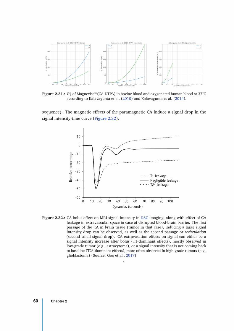
0.0 2.5 5.0 7.5 10.0 12.5 15.0 17.5 20.0Gd-DTPA concentration (mM)

0

500

1000

1500

2000

R* 2 in

bov

ine

bloo

d at

37oC

Kalavagunta et al. (2010) ISMRM abstract3T7T


0

500

1000

1500

2000

R* 2 in

bov

ine

bloo

d at

37oC

Kalavagunta et al. (2010) ISMRM presentation3T7T


0

500

1000

1500

2000

R* 2 in

oxy

gena

ted

hum

an b

lood

at 3

7oC

Kalavagunta et al. (2013) journal article3T7T

Figure 2.31.: R∗

2of Magnevist™(Gd-DTPA) in bovine blood and oxygenated human blood at 37°C

according to Kalavagunta et al. (2010) and Kalavagunta et al. (2014).

sequence). The magnetic effects of the paramagnetic CA induce a signal drop in the

signal intensity-time curve (Figure 2.32).

Figure 2.32.: CA bolus effect on MRI signal intensity in DSC imaging, along with effect of CAleakage in extravascular space in case of disrupted blood-brain barrier. The firstpassage of the CA in brain tissue (tumor in that case), inducing a large signalintensity drop can be observed, as well as the second passage or recirculation(second small signal drop). CA extravasation effects on signal can either be asignal intensity increase after bolus (T1-dominant effects), mostly observed inlow-grade tumor (e.g., astrocytoma), or a signal intensity that is not coming backto baseline (T2*-dominant effects), more often observed in high-grade tumors (e.g.,glioblastoma) (Source: Goo et al., 2017)

.

60 Chapter 2

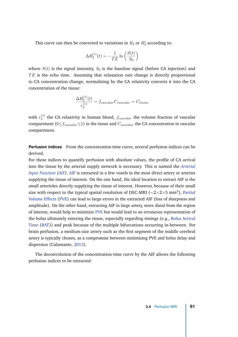
This curve can then be converted to variations in R2 or R∗

2 according to:

∆R(∗)2 (t) = − 1

TEln

(S(t)

S0

)

where S(t) is the signal intensity, S0 is the baseline signal (before CA injection) and

TE is the echo time. Assuming that relaxation rate change is directly proportional

to CA concentration change, normalizing by the CA relaxivity converts it into the CA

concentration of the tissue:

∆R(∗)2 (t)

r(∗)2

= fvascularCvascular = Ctissue

with r(∗)2 the CA relaxivity in human blood, fvascular the volume fraction of vascular

compartment (0≤fvascular≤1) in the tissue and Cvascular the CA concentration in vascular

compartment.

Perfusion indices From the concentration-time curve, several perfusion indices can be

derived.

For these indices to quantify perfusion with absolute values, the profile of CA arrival

into the tissue by the arterial supply network is necessary. This is named the Arterial

Input Function (AIF). AIF is extracted in a few voxels in the most direct artery or arteries

supplying the tissue of interest. On the one hand, the ideal location to extract AIF is the

small arterioles directly supplying the tissue of interest. However, because of their small

size with respect to the typical spatial resolution of DSC-MRI (∼2×2×5 mm3), Partial

Volume Effects (PVE) can lead to large errors in the extracted AIF (loss of sharpness and

amplitude). On the other hand, extracting AIF in large artery, more distal from the region

of interest, would help to minimize PVE but would lead to an erroneous representation of

the bolus ultimately entering the tissue, especially regarding timings (e.g., Bolus Arrival

Time (BAT)) and peak because of the multiple bifurcations occurring in-between. For

brain perfusion, a medium-size artery such as the first segment of the middle cerebral

artery is typically chosen, as a compromise between minimising PVE and bolus delay and

dispersion (Calamante, 2013).

The deconvolution of the concentration-time curve by the AIF allows the following

perfusion indices to be extracted:


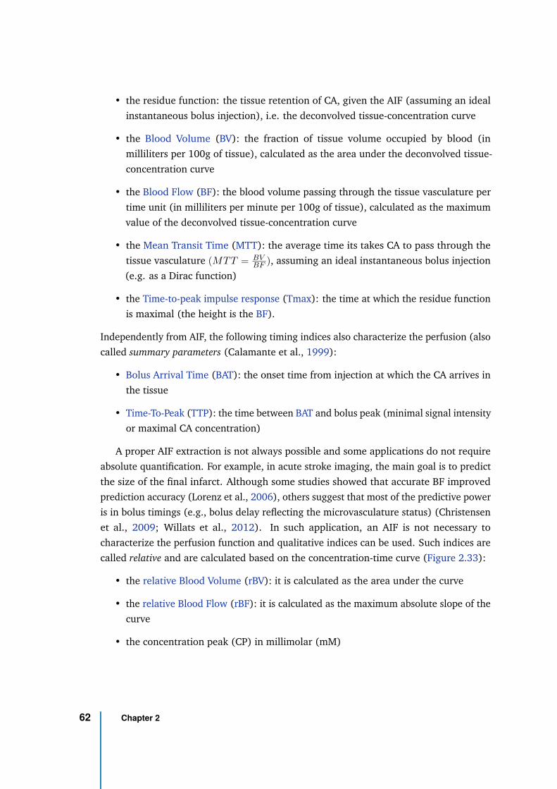
• the residue function: the tissue retention of CA, given the AIF (assuming an ideal

instantaneous bolus injection), i.e. the deconvolved tissue-concentration curve

• the Blood Volume (BV): the fraction of tissue volume occupied by blood (in

milliliters per 100g of tissue), calculated as the area under the deconvolved tissue-

concentration curve

• the Blood Flow (BF): the blood volume passing through the tissue vasculature per

time unit (in milliliters per minute per 100g of tissue), calculated as the maximum

value of the deconvolved tissue-concentration curve

• the Mean Transit Time (MTT): the average time its takes CA to pass through the

tissue vasculature (MTT = BVBF ), assuming an ideal instantaneous bolus injection

(e.g. as a Dirac function)

• the Time-to-peak impulse response (Tmax): the time at which the residue function

is maximal (the height is the BF).

Independently from AIF, the following timing indices also characterize the perfusion (also

called summary parameters (Calamante et al., 1999):

• Bolus Arrival Time (BAT): the onset time from injection at which the CA arrives in

the tissue

• Time-To-Peak (TTP): the time between BAT and bolus peak (minimal signal intensity

or maximal CA concentration)

A proper AIF extraction is not always possible and some applications do not require

absolute quantification. For example, in acute stroke imaging, the main goal is to predict

the size of the final infarct. Although some studies showed that accurate BF improved

prediction accuracy (Lorenz et al., 2006), others suggest that most of the predictive power

is in bolus timings (e.g., bolus delay reflecting the microvasculature status) (Christensen

et al., 2009; Willats et al., 2012). In such application, an AIF is not necessary to

characterize the perfusion function and qualitative indices can be used. Such indices are

called relative and are calculated based on the concentration-time curve (Figure 2.33):

• the relative Blood Volume (rBV): it is calculated as the area under the curve

• the relative Blood Flow (rBF): it is calculated as the maximum absolute slope of the

curve

• the concentration peak (CP) in millimolar (mM)

62 Chapter 2

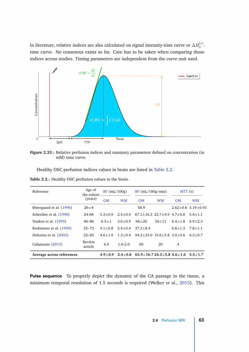
In literature, relative indices are also calculated on signal intensity-time curve or ∆R(∗)2 -

time curve. No consensus exists so far. Care has to be taken when comparing those

indices across studies. Timing parameters are independent from the curve unit used.

rCBF =dC

dt

0

rCBV = ∫ C(t)dt

BAT TTP

CP

Figure 2.33.: Relative perfusion indices and summary parameters defined on concentration (inmM) time curve.

Healthy DSC perfusion indices values in brain are listed in Table 2.2.

Table 2.2.: Healthy DSC perfusion values in the brain.

Reference Age ofthe cohort

(years)

BV (mL/100g) BF (mL/100g/min) MTT (s)

GM WM GM WM GM WM

Østergaard et al. (1996) 26±4 58.9 2.62±0.6 3.19±0.93

Schreiber et al. (1998) 24-68 5.3±0.9 2.5±0.4 67.1±16.3 23.7±4.9 4.7±0.8 5.4±1.1

Vonken et al. (1999) 40–86 6.5±1 3.6±0.9 66±20 34±11 6.4±1.8 6.9±2.3

Koshimoto et al. (1999) 25–73 4.1±0.8 2.9±0.4 37.3±8.4 6.8±1.3 7.8±1.1

Helenius et al. (2003) 22–85 4.6±1.0 1.3±0.4 94.2±23.0 19.6±5.8 3.0±0.6 4.3±0.7

Calamante (2013)Reviewarticle

4.0 1.6-2.0 60 20 4

Average across references 4.9±0.9 2.4±0.8 63.9±16.7 24.3±5.8 4.6±1.6 5.5±1.7

Pulse sequence To properly depict the dynamic of the CA passage in the tissue, a

minimum temporal resolution of 1.5 seconds is required (Welker et al., 2015). This


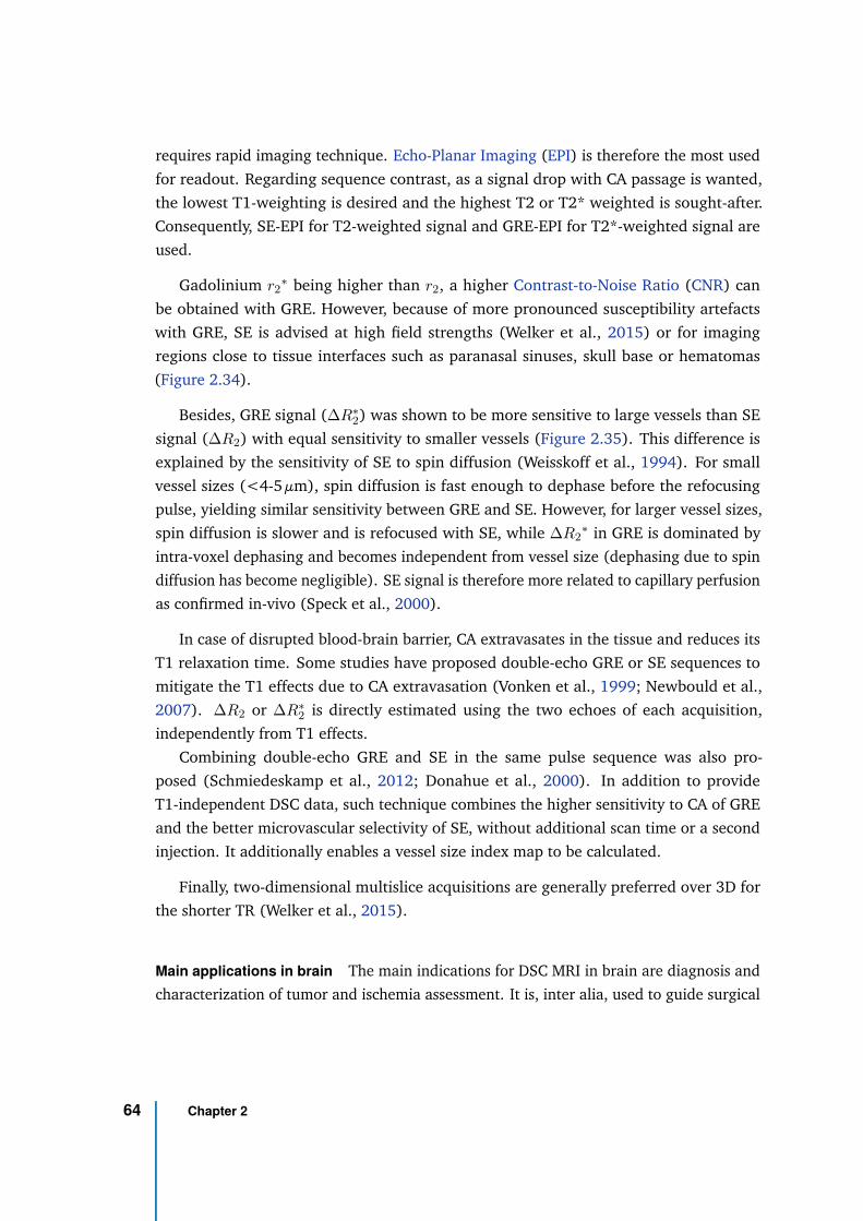
requires rapid imaging technique. Echo-Planar Imaging (EPI) is therefore the most used

for readout. Regarding sequence contrast, as a signal drop with CA passage is wanted,

the lowest T1-weighting is desired and the highest T2 or T2* weighted is sought-after.

Consequently, SE-EPI for T2-weighted signal and GRE-EPI for T2*-weighted signal are

used.

Gadolinium r2∗ being higher than r2, a higher Contrast-to-Noise Ratio (CNR) can

be obtained with GRE. However, because of more pronounced susceptibility artefacts

with GRE, SE is advised at high field strengths (Welker et al., 2015) or for imaging

regions close to tissue interfaces such as paranasal sinuses, skull base or hematomas

(Figure 2.34).

Besides, GRE signal (∆R∗

2) was shown to be more sensitive to large vessels than SE

signal (∆R2) with equal sensitivity to smaller vessels (Figure 2.35). This difference is

explained by the sensitivity of SE to spin diffusion (Weisskoff et al., 1994). For small

vessel sizes (<4-5 µm), spin diffusion is fast enough to dephase before the refocusing

pulse, yielding similar sensitivity between GRE and SE. However, for larger vessel sizes,

spin diffusion is slower and is refocused with SE, while ∆R2∗ in GRE is dominated by

intra-voxel dephasing and becomes independent from vessel size (dephasing due to spin

diffusion has become negligible). SE signal is therefore more related to capillary perfusion

as confirmed in-vivo (Speck et al., 2000).

In case of disrupted blood-brain barrier, CA extravasates in the tissue and reduces its

T1 relaxation time. Some studies have proposed double-echo GRE or SE sequences to

mitigate the T1 effects due to CA extravasation (Vonken et al., 1999; Newbould et al.,

2007). ∆R2 or ∆R∗

2 is directly estimated using the two echoes of each acquisition,

independently from T1 effects.

Combining double-echo GRE and SE in the same pulse sequence was also pro-

posed (Schmiedeskamp et al., 2012; Donahue et al., 2000). In addition to provide

T1-independent DSC data, such technique combines the higher sensitivity to CA of GRE

and the better microvascular selectivity of SE, without additional scan time or a second

injection. It additionally enables a vessel size index map to be calculated.

Finally, two-dimensional multislice acquisitions are generally preferred over 3D for

the shorter TR (Welker et al., 2015).

Main applications in brain The main indications for DSC MRI in brain are diagnosis and

characterization of tumor and ischemia assessment. It is, inter alia, used to guide surgical

64 Chapter 2

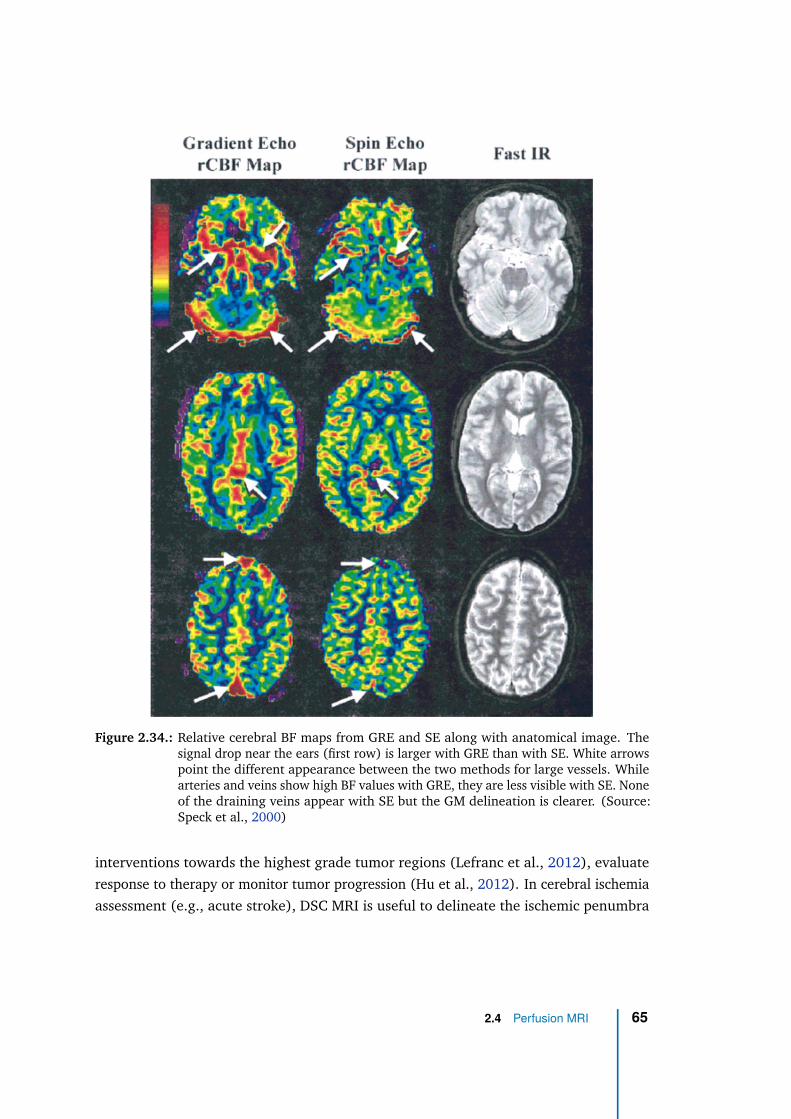
Figure 2.34.: Relative cerebral BF maps from GRE and SE along with anatomical image. Thesignal drop near the ears (first row) is larger with GRE than with SE. White arrowspoint the different appearance between the two methods for large vessels. Whilearteries and veins show high BF values with GRE, they are less visible with SE. Noneof the draining veins appear with SE but the GM delineation is clearer. (Source:Speck et al., 2000)

interventions towards the highest grade tumor regions (Lefranc et al., 2012), evaluate

response to therapy or monitor tumor progression (Hu et al., 2012). In cerebral ischemia

assessment (e.g., acute stroke), DSC MRI is useful to delineate the ischemic penumbra


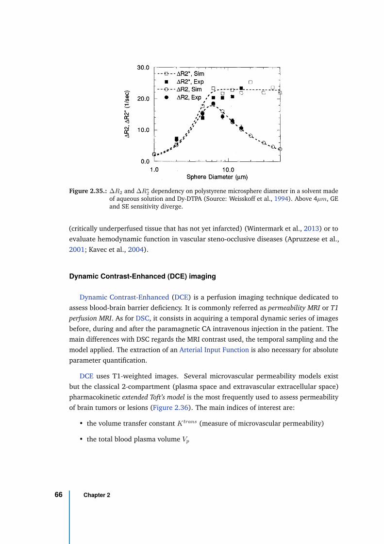
Figure 2.35.: ∆R2 and ∆R∗

2dependency on polystyrene microsphere diameter in a solvent made

of aqueous solution and Dy-DTPA (Source: Weisskoff et al., 1994). Above 4µm, GEand SE sensitivity diverge.

(critically underperfused tissue that has not yet infarcted) (Wintermark et al., 2013) or to

evaluate hemodynamic function in vascular steno-occlusive diseases (Apruzzese et al.,

2001; Kavec et al., 2004).

Dynamic Contrast-Enhanced (DCE) imaging

Dynamic Contrast-Enhanced (DCE) is a perfusion imaging technique dedicated to

assess blood-brain barrier deficiency. It is commonly referred as permeability MRI or T1

perfusion MRI. As for DSC, it consists in acquiring a temporal dynamic series of images

before, during and after the paramagnetic CA intravenous injection in the patient. The

main differences with DSC regards the MRI contrast used, the temporal sampling and the

model applied. The extraction of an Arterial Input Function is also necessary for absolute

parameter quantification.

DCE uses T1-weighted images. Several microvascular permeability models exist

but the classical 2-compartment (plasma space and extravascular extracellular space)

pharmacokinetic extended Toft’s model is the most frequently used to assess permeability

of brain tumors or lesions (Figure 2.36). The main indices of interest are:

• the volume transfer constant Ktrans (measure of microvascular permeability)

• the total blood plasma volume Vp

66 Chapter 2

• the total extravascular extracelluar volume Ve

• the rate constant from extravascular extracellular space to plasma space Kep =

Ktrans/Ve

Figure 2.36.: Example of 2-compartment pharmacokinetic models of DCE and derived perfusionparameters, Toft’s model being the most frequently used. The difference betweenToft and extended Toft’s models is that the latest additionally estimate the bloodplasma volume Vp (source: Gaddikeri et al., 2016)

.

Because of the higher relaxivity r2 of Gd-based CA compared to r1, indices directly

related to perfusion (e.g. BF, BV, MTT) are preferably estimated based on T2-weighted

images given the consequent higher sensitivity. When permeability needs to be assessed,

for instance to delineate tumor or characterize vessel functionality in neoangiogenesis,

T1-weighted images are preferred over T2-weighted EPI sequences, which potentially

come with limited spatial resolution and image distortion. Nonetheless, DSC MRI can

provide indices of CA extravasation (Schmainda et al., 2004). Conversely, a few studies

also showed that perfusion-related indices could also be extracted from T1-weighted

dynamic image series, providing prior acquisition of a quantitative T1 map. Table 2.3 lists

those studies and the BF and BV obtained in brain. (Haroon et al., 2007) and (Zakariaee

et al., 2018) acquired both DCE and DSC protocols in patients with brain tumors. An

example of the obtained BV and BF maps are presented in Figure 2.37 and a comparison

of values in WM, GM and tumors is presented in Table 2.4.


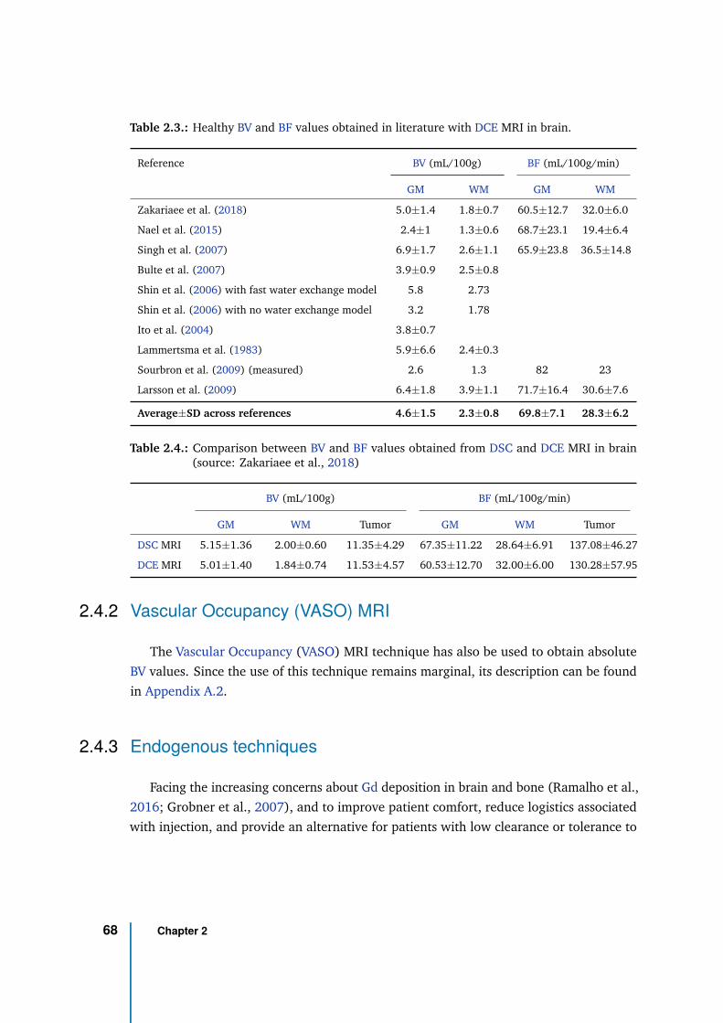
Table 2.3.: Healthy BV and BF values obtained in literature with DCE MRI in brain.

Reference BV (mL/100g) BF (mL/100g/min)

GM WM GM WM

Zakariaee et al. (2018) 5.0±1.4 1.8±0.7 60.5±12.7 32.0±6.0

Nael et al. (2015) 2.4±1 1.3±0.6 68.7±23.1 19.4±6.4

Singh et al. (2007) 6.9±1.7 2.6±1.1 65.9±23.8 36.5±14.8

Bulte et al. (2007) 3.9±0.9 2.5±0.8

Shin et al. (2006) with fast water exchange model 5.8 2.73

Shin et al. (2006) with no water exchange model 3.2 1.78

Ito et al. (2004) 3.8±0.7

Lammertsma et al. (1983) 5.9±6.6 2.4±0.3

Sourbron et al. (2009) (measured) 2.6 1.3 82 23

Larsson et al. (2009) 6.4±1.8 3.9±1.1 71.7±16.4 30.6±7.6

Average±SD across references 4.6±1.5 2.3±0.8 69.8±7.1 28.3±6.2

Table 2.4.: Comparison between BV and BF values obtained from DSC and DCE MRI in brain(source: Zakariaee et al., 2018)

BV (mL/100g) BF (mL/100g/min)

GM WM Tumor GM WM Tumor

DSC MRI 5.15±1.36 2.00±0.60 11.35±4.29 67.35±11.22 28.64±6.91 137.08±46.27

DCE MRI 5.01±1.40 1.84±0.74 11.53±4.57 60.53±12.70 32.00±6.00 130.28±57.95

2.4.2 Vascular Occupancy (VASO) MRI

The Vascular Occupancy (VASO) MRI technique has also be used to obtain absolute

BV values. Since the use of this technique remains marginal, its description can be found

in Appendix A.2.

2.4.3 Endogenous techniques

Facing the increasing concerns about Gd deposition in brain and bone (Ramalho et al.,

2016; Grobner et al., 2007), and to improve patient comfort, reduce logistics associated

with injection, and provide an alternative for patients with low clearance or tolerance to

68 Chapter 2

Figure 2.37.: Comparison of BV and BF maps obtained from typical DSC (T2*-weighted images)and DCE (T1-weighted images) protocolsDCE (source: Zakariaee et al., 2018)

.

Gd, researchers have looked at endogenous contrast mechanism to evaluate perfusion

without CA injection.

Arterial Spin Labeling (ASL)

Arterial Spin Labeling (ASL) is the most famous endogenous method for perfusion

imaging (Alsop et al., 2015). The contrast agent is replaced by magnetization-tagged

blood water molecules flowing to the tissue of interest. Indeed, for ASL in brain, RF

pulses are applied right below the brain, to invert the magnetization of arterial blood

water molecules flowing into the brain, and after a Post-Label Delay (PLD), an image


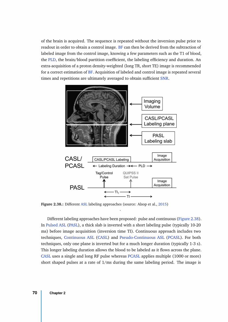
of the brain is acquired. The sequence is repeated without the inversion pulse prior to

readout in order to obtain a control image. BF can then be derived from the subtraction of

labeled image from the control image, knowing a few parameters such as the T1 of blood,

the PLD, the brain/blood partition coefficient, the labeling efficiency and duration. An

extra-acquisition of a proton density-weighted (long TR, short TE) image is recommended

for a correct estimation of BF. Acquisition of labeled and control image is repeated several

times and repetitions are ultimately averaged to obtain sufficient SNR.

Figure 2.38.: Different ASL labeling approaches (source: Alsop et al., 2015).

Different labeling approaches have been proposed: pulse and continuous (Figure 2.38).

In Pulsed ASL (PASL), a thick slab is inverted with a short labeling pulse (typically 10-20

ms) before image acquisition (inversion time TI). Continuous approach includes two

techniques, Continuous ASL (CASL) and Pseudo-Continuous ASL (PCASL). For both

techniques, only one plane is inverted but for a much longer duration (typically 1-3 s).

This longer labeling duration allows the blood to be labeled as it flows across the plane.

CASL uses a single and long RF pulse whereas PCASL applies multiple (1000 or more)

short shaped pulses at a rate of 1/ms during the same labeling period. The image is

70 Chapter 2

acquired after a PLD.

PCASL provides superior labeling efficiency than PASL and CASL and is recommended

for cerebral clinical use (Alsop et al., 2015). The volume of blood labeled is larger with

continuous than with pulsed approaches. In PASL, the volume of the labeling slab is

limited by the efficient spatial coverage of the transmit coil. Given that it rarely exceeds

20cm in inferior-superior direction and that arterial blood supply to brain has a mean

velocity of 20 cm/s, the equivalent labeling duration relative to continuous approaches

would be around 1 second.

To quantify Blood Flow (BF) in brain from PCASL data acquired with a single PLD,

the following model can be used (Buxton et al., 1998):

BF [mL/100g/min] =6000 · λ · (Scontrol − Slabel) · eP LD/T blood

1

2α · T blood1 SP D · (1 − e−τ/T blood

1 )(2.24)

with:

• λ: the brain/blood partition coefficient in mL/g (generally set to 0.9 mL/g)

• Scontrol: the signal intensity (usually averaged across repetitions) in the control

image

• Slabel: the signal intensity (usually averaged across repetitions) in the labeled image

• PLD: the Post-Label Delay

• T blood1 : the longitudinal relaxation time of blood in seconds (e.g., 1.480, 1.649 and

2.087 s at 1.5T, 3T and 7T (Zhang et al., 2013)), which depends on the subject’s

hematocrit concentration

• α: the labeling efficiency (generally set to 0.85 for PCASL)

• SP D: the signal intensity of a proton density-weighted image

• τ : the label duration

This model assumes that the entire labeled blood bolus is delivered to the target tissue,

that there is no outflow of labeled blood water and that the relaxation of labeled spins is

defined by blood T1 only.

Perfusion parameters quantified with single PLD/TI acquisition depend on the PLD/TI

value used. Using multiple PLD/TI acquisitions, the Arterial Transit Time (ATT), which is


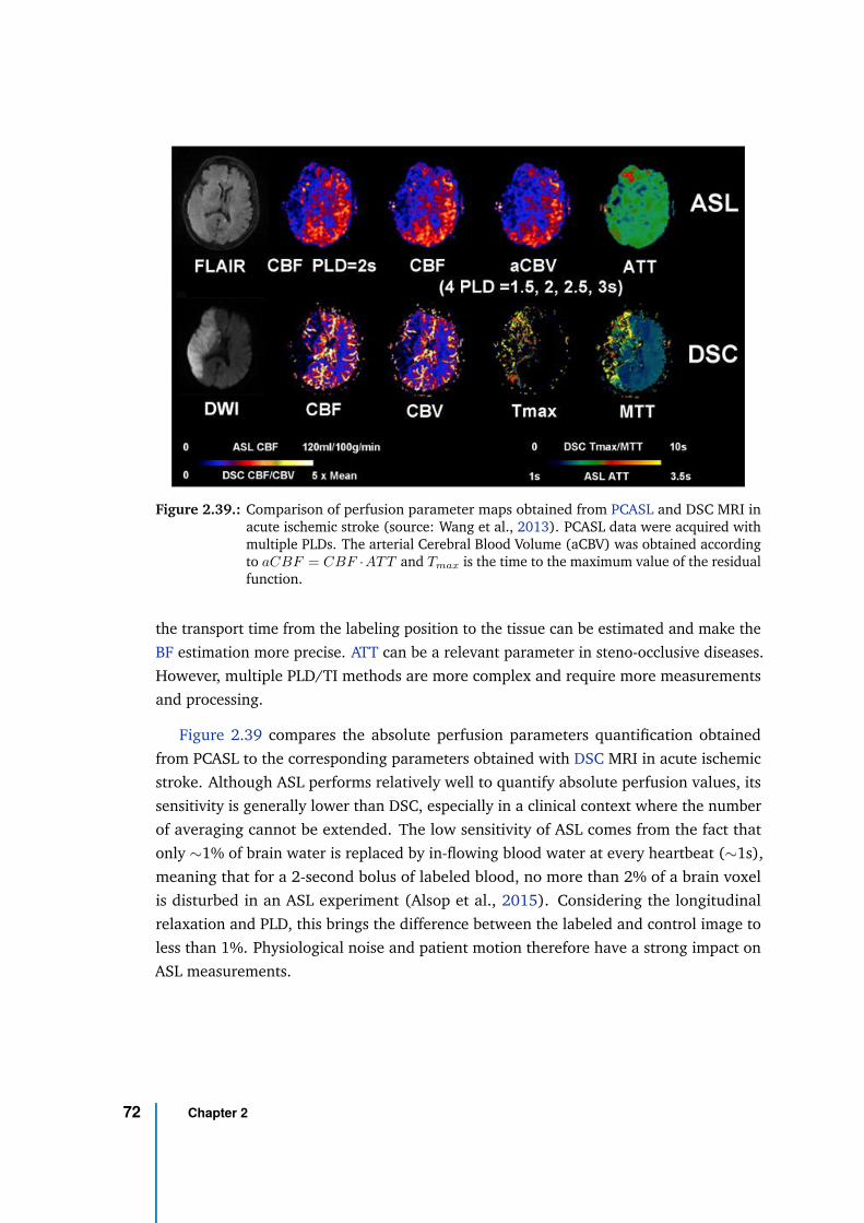
Figure 2.39.: Comparison of perfusion parameter maps obtained from PCASL and DSC MRI inacute ischemic stroke (source: Wang et al., 2013). PCASL data were acquired withmultiple PLDs. The arterial Cerebral Blood Volume (aCBV) was obtained accordingto aCBF = CBF ·ATT and Tmax is the time to the maximum value of the residualfunction.

the transport time from the labeling position to the tissue can be estimated and make the

BF estimation more precise. ATT can be a relevant parameter in steno-occlusive diseases.

However, multiple PLD/TI methods are more complex and require more measurements

and processing.

Figure 2.39 compares the absolute perfusion parameters quantification obtained

from PCASL to the corresponding parameters obtained with DSC MRI in acute ischemic

stroke. Although ASL performs relatively well to quantify absolute perfusion values, its

sensitivity is generally lower than DSC, especially in a clinical context where the number

of averaging cannot be extended. The low sensitivity of ASL comes from the fact that

only ∼1% of brain water is replaced by in-flowing blood water at every heartbeat (∼1s),

meaning that for a 2-second bolus of labeled blood, no more than 2% of a brain voxel

is disturbed in an ASL experiment (Alsop et al., 2015). Considering the longitudinal

relaxation and PLD, this brings the difference between the labeled and control image to

less than 1%. Physiological noise and patient motion therefore have a strong impact on

ASL measurements.

72 Chapter 2

To address that, a common strategy is to use background suppression to reduce as

much as possible the signal coming from the stationary tissue. Background suppression

strategies typically use initial selective saturation pulse and a carefully calculated inversion

pulse timing to ensure that the magnetization of stationary tissue is close to 0 at the time

of image acquisition (Maleki et al., 2012).

Regarding the readout, 3D segmented multi-echo RARE (Rapid Acquisition With

Relaxation Enhancement) (Hennig et al., 1986; Hennig, 1988) stack of spirals or 3D

segmented GRASE (GRadient- And Spine-Echo) (Feinberg et al., 1991) sequences are

recommended because of their SNR efficiency and good compatibility with background

suppression as they use only one excitation by TR, unlike 2D multi-slice strategies which

can be an alternative (single-shot EPI or spiral Fast Spin-Echo) (Alsop et al., 2015).

ASL could therefore be advantageous over DSC in the sense that it does not require

the injection of an exogenous CA, which is a non-negligible asset for patient low CA

clearance capacities or intolerant to CA. In addition, the acquisition time can be traded

for SNR through multiple averages, which cannot be with DSC. A longer scan time is

nonetheless required to reach the sensitivity of DSC. Another disadvantage of ASL, which

is particularly relevant at UHF with regards to SAR limits, is the high-energy deposition

of the pulse sequences and the high inversion efficiency required.

Intra-Voxel Incoherent Motion (IVIM)

Diffusion MRI Thermal agitation in any living body induces a random motion (or Brow-

nian motion) of the molecules. In particular, water molecules in human body (80%)

naturally moves in the tissue. This displacement is characterized by mean value of:

< r2 >=√

6D∆

where D is the coefficient of diffusion of H2O in the tissue. ∆ is the time of diffusion and

the factor 6 accounts for the degrees of freedom in 3D.

It is possible to make the MRI signal sensitive to the water molecule diffusion, yielding

Diffusion-Weighted Imaging (DWI). The most frequently used sequence to do so is the

spin-echo (Stejskal et al., 1965). Magnetic field gradients are added before and after

the 180° RF pulse. Figure 2.40 presents the theoretical cases of a voxel including two

proton spins staying at the same position (first row) and one proton spin staying still


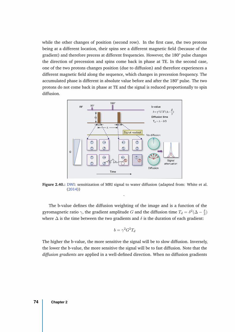
while the other changes of position (second row). In the first case, the two protons

being at a different location, their spins see a different magnetic field (because of the

gradient) and therefore precess at different frequencies. However, the 180° pulse changes

the direction of precession and spins come back in phase at TE. In the second case,

one of the two protons changes position (due to diffusion) and therefore experiences a

different magnetic field along the sequence, which changes in precession frequency. The

accumulated phase is different in absolute value before and after the 180° pulse. The two

protons do not come back in phase at TE and the signal is reduced proportionally to spin

diffusion.

b-value

b = γ 2G2δ 2(Δ −δ

3)

Figure 2.40.: DWI: sensitization of MRI signal to water diffusion (adapted from: White et al.(2014))

.

The b-value defines the diffusion weighting of the image and is a function of the

gyromagnetic ratio γ, the gradient amplitude G and the diffusion time Td = δ2(∆ − δ3)

where ∆ is the time between the two gradients and δ is the duration of each gradient:

b = γ2G2Td

The higher the b-value, the more sensitive the signal will be to slow diffusion. Inversely,

the lower the b-value, the more sensitive the signal will be to fast diffusion. Note that the

diffusion gradients are applied in a well-defined direction. When no diffusion gradients

74 Chapter 2

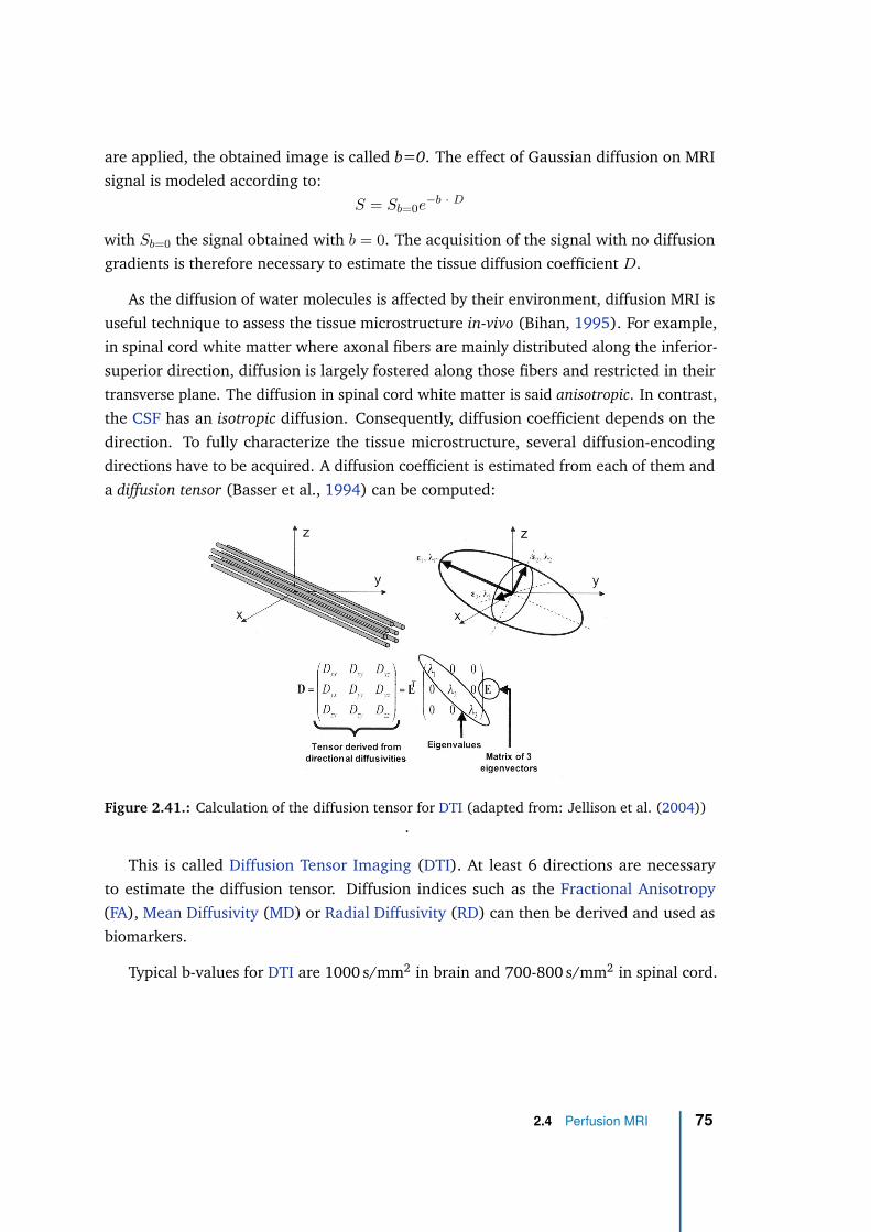
are applied, the obtained image is called b=0. The effect of Gaussian diffusion on MRI

signal is modeled according to:

S = Sb=0e−b · D

with Sb=0 the signal obtained with b = 0. The acquisition of the signal with no diffusion

gradients is therefore necessary to estimate the tissue diffusion coefficient D.

As the diffusion of water molecules is affected by their environment, diffusion MRI is

useful technique to assess the tissue microstructure in-vivo (Bihan, 1995). For example,

in spinal cord white matter where axonal fibers are mainly distributed along the inferior-

superior direction, diffusion is largely fostered along those fibers and restricted in their

transverse plane. The diffusion in spinal cord white matter is said anisotropic. In contrast,

the CSF has an isotropic diffusion. Consequently, diffusion coefficient depends on the

direction. To fully characterize the tissue microstructure, several diffusion-encoding

directions have to be acquired. A diffusion coefficient is estimated from each of them and

a diffusion tensor (Basser et al., 1994) can be computed:

Figure 2.41.: Calculation of the diffusion tensor for DTI (adapted from: Jellison et al. (2004)).

This is called Diffusion Tensor Imaging (DTI). At least 6 directions are necessary

to estimate the diffusion tensor. Diffusion indices such as the Fractional Anisotropy

(FA), Mean Diffusivity (MD) or Radial Diffusivity (RD) can then be derived and used as

biomarkers.

Typical b-values for DTI are 1000 s/mm2 in brain and 700-800 s/mm2 in spinal cord.


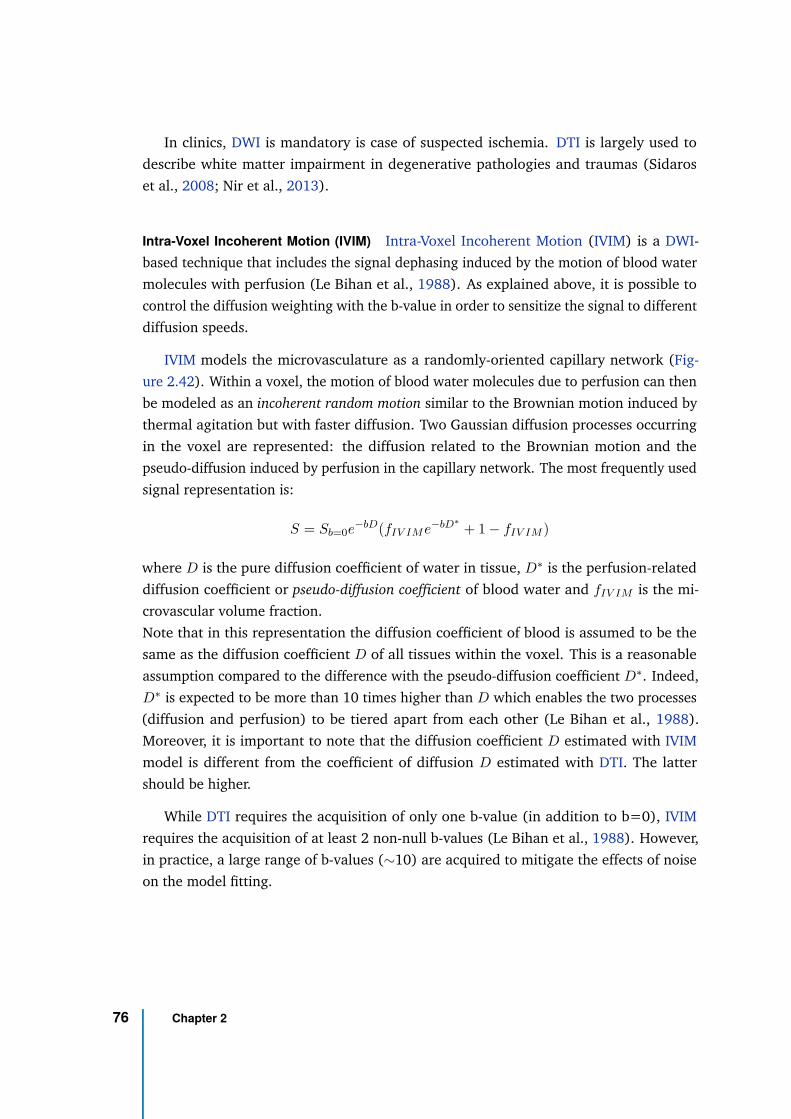
In clinics, DWI is mandatory is case of suspected ischemia. DTI is largely used to

describe white matter impairment in degenerative pathologies and traumas (Sidaros

et al., 2008; Nir et al., 2013).

Intra-Voxel Incoherent Motion (IVIM) Intra-Voxel Incoherent Motion (IVIM) is a DWI-

based technique that includes the signal dephasing induced by the motion of blood water

molecules with perfusion (Le Bihan et al., 1988). As explained above, it is possible to

control the diffusion weighting with the b-value in order to sensitize the signal to different

diffusion speeds.

IVIM models the microvasculature as a randomly-oriented capillary network (Fig-

ure 2.42). Within a voxel, the motion of blood water molecules due to perfusion can then

be modeled as an incoherent random motion similar to the Brownian motion induced by

thermal agitation but with faster diffusion. Two Gaussian diffusion processes occurring

in the voxel are represented: the diffusion related to the Brownian motion and the

pseudo-diffusion induced by perfusion in the capillary network. The most frequently used

signal representation is:

S = Sb=0e−bD(fIV IM e−bD∗

+ 1 − fIV IM )

where D is the pure diffusion coefficient of water in tissue, D∗ is the perfusion-related

diffusion coefficient or pseudo-diffusion coefficient of blood water and fIV IM is the mi-

crovascular volume fraction.

Note that in this representation the diffusion coefficient of blood is assumed to be the

same as the diffusion coefficient D of all tissues within the voxel. This is a reasonable

assumption compared to the difference with the pseudo-diffusion coefficient D∗. Indeed,

D∗ is expected to be more than 10 times higher than D which enables the two processes

(diffusion and perfusion) to be tiered apart from each other (Le Bihan et al., 1988).

Moreover, it is important to note that the diffusion coefficient D estimated with IVIM

model is different from the coefficient of diffusion D estimated with DTI. The latter

should be higher.

While DTI requires the acquisition of only one b-value (in addition to b=0), IVIM

requires the acquisition of at least 2 non-null b-values (Le Bihan et al., 1988). However,

in practice, a large range of b-values (∼10) are acquired to mitigate the effects of noise

on the model fitting.

76 Chapter 2

𝑆 = 𝑆!𝑒"#$(𝑓%&%'𝑒

"#$∗

+ 1 − 𝑓%&%')

Random walk of blood water within

capillary network

MRI voxel ln(S)

D

b-value

Signal dephasing

induced by

perfusion

D: pure diffusion coefficient within tissue

D*: perfusion-related diffusion (or pseudo-diffusion) coefficient

fIVIM: microvascular volume fraction

Figure 2.42.: Intra-Voxel Incoherent Motion (IVIM) model and signal representation (adaptedfrom Nicholas Theodore, M.D.)

.

Indeed, the bi-exponential representation has been showed to be very sensitive to noise

(Novikov et al., 2018) and people have been suspicious about the feasability to quantify

IVIM indices in the central nervous system. In 1992, King et al. (1992) investigated the

reliability of IVIM least-square fit in a rat brain and concluded that IVIM indices could

not be quantified reliably because of the difficulty to fit biexponential representation. In

2019, Milani et al. (2019) showed with simulations for kidney perfusion quantification

that fIV IM estimation reliability strongly decreased with the ratio D ∗ /D. Given that

perfusion velocity changes during cardiac cycle (e.g., up to a factor 2 in the anterior

cerebral artery (Federau et al., 2013), it would therefore be recommended to acquire data

at the peak of perfusion velocity. They confirmed this result in-vivo with maps showing

less inconsistent values and more consistent anatomical details when acquired at the

peak of perfusion velocity. Phase-contrast imaging sequence of the renal artery was used

to determine this time.

Healthy values and pathological applications IVIM values reported in literature for

healthy brain GM and WM are collected in Table 2.5. Large SD across studies can be

observed for fIV IM and D∗, attesting of the instability of the biexponential fit or of the

strong dependence on acquisition parameters. Estimation of D is more robust.

Healthy IVIM values in brain have also shown large variability depending on the b-

value distribution (Hu et al., 2020) and the fitting method (two-step or one-step approach).


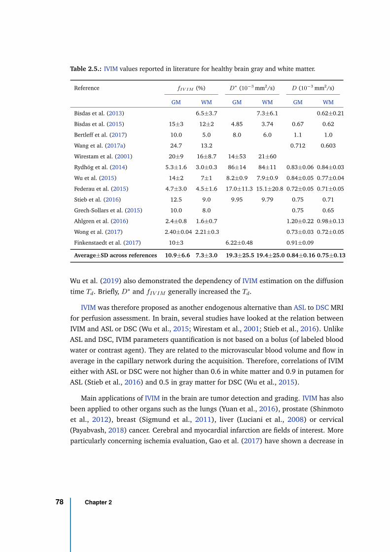
Table 2.5.: IVIM values reported in literature for healthy brain gray and white matter.

Reference fIV IM (%) D∗ (10−3 mm2/s) D (10

−3 mm2/s)

GM WM GM WM GM WM

Bisdas et al. (2013) 6.5±3.7 7.3±6.1 0.62±0.21

Bisdas et al. (2015) 15±3 12±2 4.85 3.74 0.67 0.62

Bertleff et al. (2017) 10.0 5.0 8.0 6.0 1.1 1.0

Wang et al. (2017a) 24.7 13.2 0.712 0.603

Wirestam et al. (2001) 20±9 16±8.7 14±53 21±60

Rydhög et al. (2014) 5.3±1.6 3.0±0.3 86±14 84±11 0.83±0.06 0.84±0.03

Wu et al. (2015) 14±2 7±1 8.2±0.9 7.9±0.9 0.84±0.05 0.77±0.04

Federau et al. (2015) 4.7±3.0 4.5±1.6 17.0±11.3 15.1±20.8 0.72±0.05 0.71±0.05

Stieb et al. (2016) 12.5 9.0 9.95 9.79 0.75 0.71

Grech-Sollars et al. (2015) 10.0 8.0 0.75 0.65

Ahlgren et al. (2016) 2.4±0.8 1.6±0.7 1.20±0.22 0.98±0.13

Wong et al. (2017) 2.40±0.04 2.21±0.3 0.73±0.03 0.72±0.05

Finkenstaedt et al. (2017) 10±3 6.22±0.48 0.91±0.09

Average±SD across references 10.9±6.6 7.3±3.0 19.3±25.5 19.4±25.0 0.84±0.16 0.75±0.13

Wu et al. (2019) also demonstrated the dependency of IVIM estimation on the diffusion

time Td. Briefly, D∗ and fIV IM generally increased the Td.

IVIM was therefore proposed as another endogenous alternative than ASL to DSC MRI

for perfusion assessment. In brain, several studies have looked at the relation between

IVIM and ASL or DSC (Wu et al., 2015; Wirestam et al., 2001; Stieb et al., 2016). Unlike

ASL and DSC, IVIM parameters quantification is not based on a bolus (of labeled blood

water or contrast agent). They are related to the microvascular blood volume and flow in

average in the capillary network during the acquisition. Therefore, correlations of IVIM

either with ASL or DSC were not higher than 0.6 in white matter and 0.9 in putamen for

ASL (Stieb et al., 2016) and 0.5 in gray matter for DSC (Wu et al., 2015).

Main applications of IVIM in the brain are tumor detection and grading. IVIM has also

been applied to other organs such as the lungs (Yuan et al., 2016), prostate (Shinmoto

et al., 2012), breast (Sigmund et al., 2011), liver (Luciani et al., 2008) or cervical

(Payabvash, 2018) cancer. Cerebral and myocardial infarction are fields of interest. More

particularly concerning ischemia evaluation, Gao et al. (2017) have shown a decrease in

78 Chapter 2

fIV IM , D∗ and D in the ischemic stroke hemisphere compared to contralateral side in a

canine stroke model. Diagnosis performance of IVIM imaging in acute stroke was assessed

in a clinical setting (Federau et al., 2014). fIV IM was found to be significantly reduced

in the visible infarct (2.6% vs. 5.6% in the contralateral side) but with a large variation

of the values across subjects (standard-deviation of 1.9% and 2.5% in contralateral side),

in agreement with the large range of values observed in the literature (Table 2.5).

2.4.4 State of the art in spinal cord

Measuring perfusion in spinal cord tissue has elicited the interest of researchers and

neurosurgeons seeking techniques to assess spinal cord tissue integrity and viability after

traumatic injury, chronic compression or for surgical planning.

Interesting work has first been done in mice using PASL at 11.75T. Duhamel et al.

(2008) were able to reveal the higher BF of gray matter compared to white matter at C3

and C6 vertebral level with 50 averages and acquisition time of 34 minutes per level for a

spatial resolution of 133×133 µm2 (Figure 2.43). BF was estimated at 226 mL/100g/min

in GM cortex, around 330 mL/100g/min in spinal cord GM, and 146 mL/100g/min in

spinal cord WM, yielding a GM/WM ratio of 2.3. However, even with long acquisition

time, the SNR of an 11.75T magnet, the large GM/WM volume ratio of the mouse spinal

cord (compared to human) and anesthetized subjects, BF measurements within GM and

WM showed up to 30% and 77% of in-ROI variations, and up to 16% and 40% of group

variations, respectively. Those variations in a well controlled set-up attest to the challenge

to measure perfusion in human spinal cord with MRI. Furthermore, a lower perfusion was

measured in average at L1 vertebral level, compared to C3 (285 vs. 310 mL/100g/min in

GM and 100 vs. 121 ml/100g/min in WM) (Duhamel et al., 2009).

Up to one year ago, clinical work has not gotten past the barrier of conference

proceedings.

Nair et al. (2010) evaluated a PASL technique in human at 3T. They were able to show

sensitivity to perfusion in cord ROI using multiple inversion times but BF mapping was

not reliable with an average of 26±11 mL/100g/min in cord (Figure 2.44a). Girard et al.

(2013) upgraded the PASL technique in human spinal cord at 1.5T with an additional

preparation dedicated to suppress signal from inflowing CSF using a global inversion

pulse and labeling at the CSF nulling point. They also compared it to PCASL which

showed a better sensitivity. Additional interesting features were the electrocardiogram


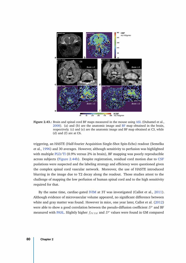
Figure 2.43.: Brain and spinal cord BF maps measured in the mouse using ASL (Duhamel et al.,2008). (a) and (b) are the anatomic image and BF map obtained in the brain,respectively. (c) and (e) are the anatomic image and BF map obtained at C3, while(d) and (f) are at C6.

triggering, an HASTE (Half-fourier Acquisition Single-Shot Spin-Echo) readout (Semelka

et al., 1996) and 30 averages. However, although sensitivity to perfusion was highlighted

with multiple PLD/TI (0.9% versus 2% in brain), BF mapping was poorly reproducible

across subjects (Figure 2.44b). Despite registration, residual cord motion due to CSF

puslations were suspected and the labeling strategy and efficiency were questioned given

the complex spinal cord vascular network. Moreover, the use of HASTE introduced

blurring in the image due to T2 decay along the readout. Those studies attest to the

challenge of mapping the low perfusion of human spinal cord and to the high sensitivity

required for that.

By the same time, cardiac-gated IVIM at 3T was investigated (Callot et al., 2011).

Although evidence of microvascular volume appeared, no significant difference between

white and gray matter was found. However in mice, one year later, Callot et al. (2012)

were able to show a good correlation between the pseudo-diffusion coefficient D∗ and BF

measured with PASL. Slightly higher fIV IM and D∗ values were found in GM compared

80 Chapter 2

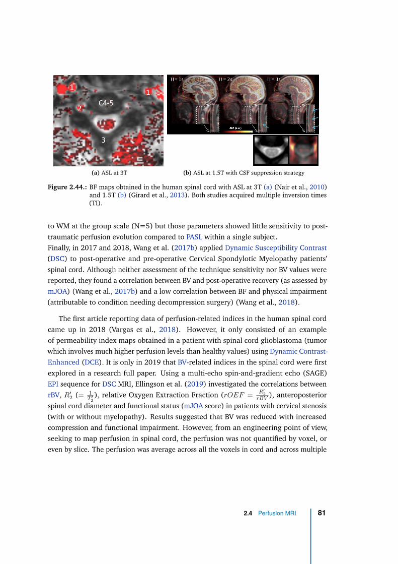
(a) ASL at 3T (b) ASL at 1.5T with CSF suppression strategy

Figure 2.44.: BF maps obtained in the human spinal cord with ASL at 3T (a) (Nair et al., 2010)and 1.5T (b) (Girard et al., 2013). Both studies acquired multiple inversion times(TI).

to WM at the group scale (N=5) but those parameters showed little sensitivity to post-

traumatic perfusion evolution compared to PASL within a single subject.

Finally, in 2017 and 2018, Wang et al. (2017b) applied Dynamic Susceptibility Contrast

(DSC) to post-operative and pre-operative Cervical Spondylotic Myelopathy patients’

spinal cord. Although neither assessment of the technique sensitivity nor BV values were

reported, they found a correlation between BV and post-operative recovery (as assessed by

mJOA) (Wang et al., 2017b) and a low correlation between BF and physical impairment

(attributable to condition needing decompression surgery) (Wang et al., 2018).

The first article reporting data of perfusion-related indices in the human spinal cord

came up in 2018 (Vargas et al., 2018). However, it only consisted of an example

of permeability index maps obtained in a patient with spinal cord glioblastoma (tumor

which involves much higher perfusion levels than healthy values) using Dynamic Contrast-

Enhanced (DCE). It is only in 2019 that BV-related indices in the spinal cord were first

explored in a research full paper. Using a multi-echo spin-and-gradient echo (SAGE)

EPI sequence for DSC MRI, Ellingson et al. (2019) investigated the correlations between

rBV, R′

2 (= 1T ′

2

), relative Oxygen Extraction Fraction (rOEF =R′

2

rBV ), anteroposterior

spinal cord diameter and functional status (mJOA score) in patients with cervical stenosis

(with or without myelopathy). Results suggested that BV was reduced with increased

compression and functional impairment. However, from an engineering point of view,

seeking to map perfusion in spinal cord, the perfusion was not quantified by voxel, or

even by slice. The perfusion was average across all the voxels in cord and across multiple


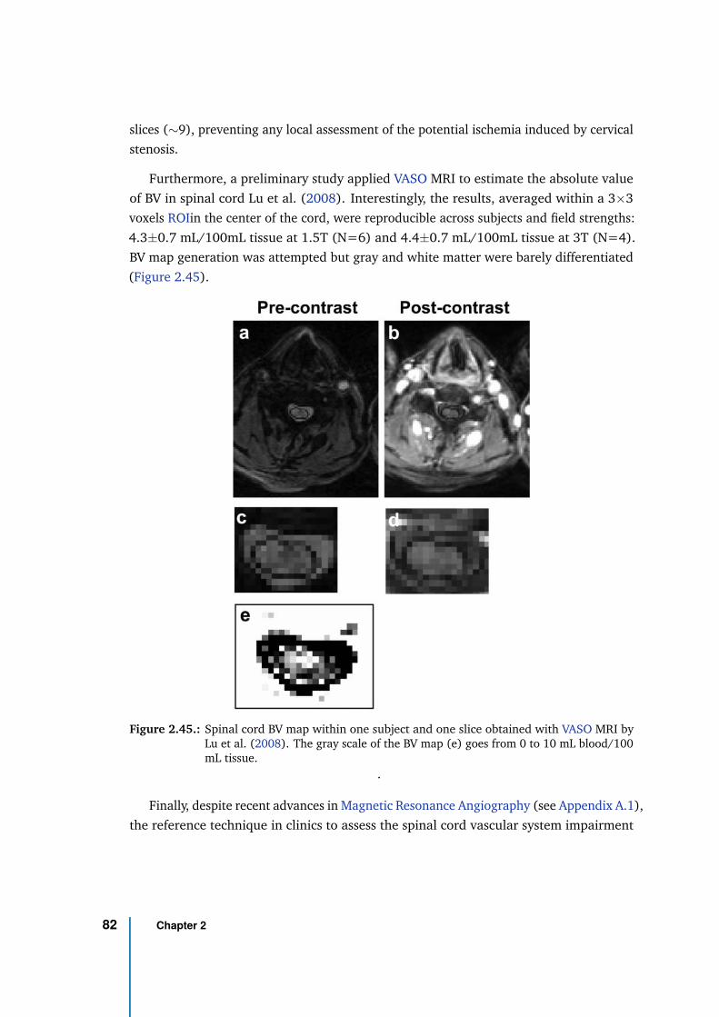
slices (∼9), preventing any local assessment of the potential ischemia induced by cervical

stenosis.

Furthermore, a preliminary study applied VASO MRI to estimate the absolute value

of BV in spinal cord Lu et al. (2008). Interestingly, the results, averaged within a 3×3

voxels ROIin the center of the cord, were reproducible across subjects and field strengths:

4.3±0.7 mL/100mL tissue at 1.5T (N=6) and 4.4±0.7 mL/100mL tissue at 3T (N=4).

BV map generation was attempted but gray and white matter were barely differentiated

(Figure 2.45).

Figure 2.45.: Spinal cord BV map within one subject and one slice obtained with VASO MRI byLu et al. (2008). The gray scale of the BV map (e) goes from 0 to 10 mL blood/100mL tissue.

.

Finally, despite recent advances in Magnetic Resonance Angiography (see Appendix A.1),

the reference technique in clinics to assess the spinal cord vascular system impairment

82 Chapter 2

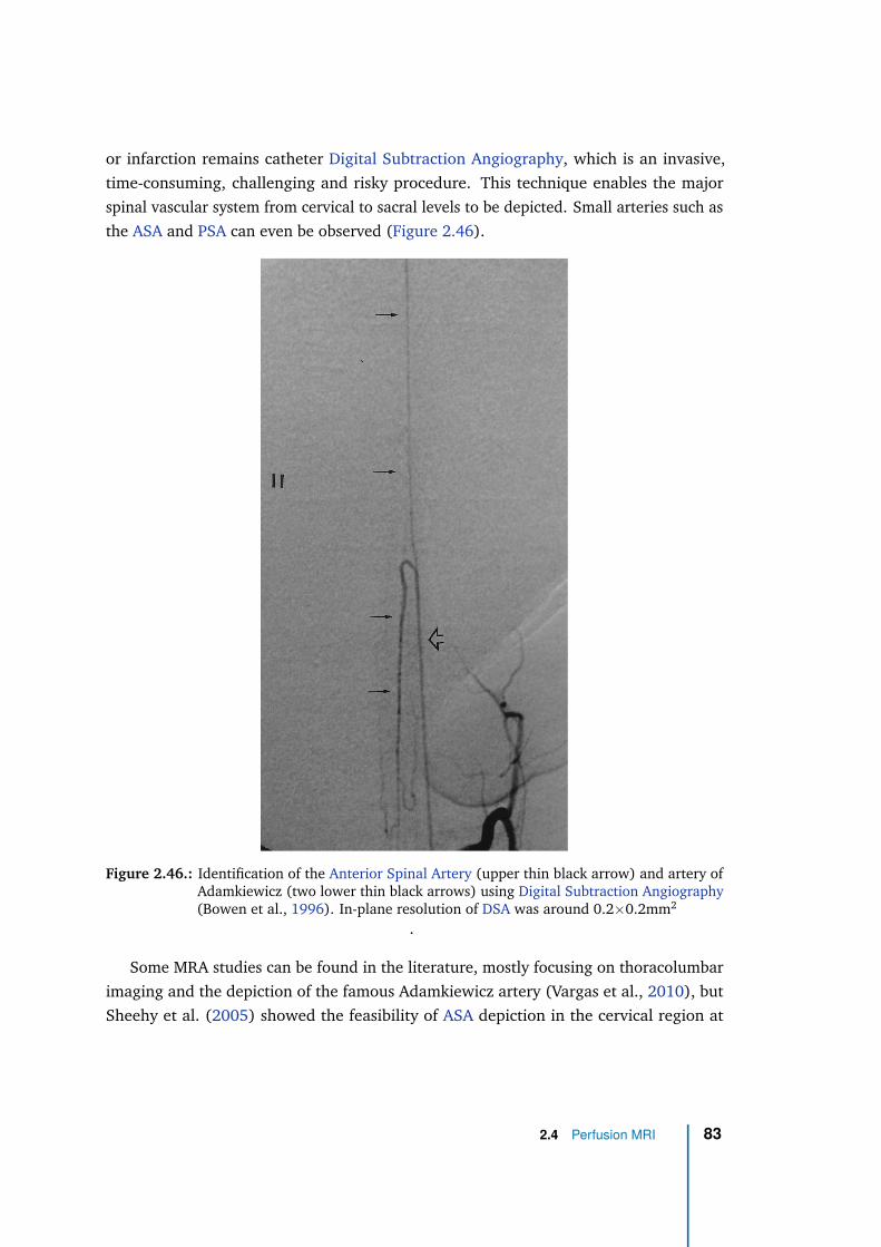
or infarction remains catheter Digital Subtraction Angiography, which is an invasive,

time-consuming, challenging and risky procedure. This technique enables the major

spinal vascular system from cervical to sacral levels to be depicted. Small arteries such as

the ASA and PSA can even be observed (Figure 2.46).

Figure 2.46.: Identification of the Anterior Spinal Artery (upper thin black arrow) and artery ofAdamkiewicz (two lower thin black arrows) using Digital Subtraction Angiography(Bowen et al., 1996). In-plane resolution of DSA was around 0.2×0.2mm2

.

Some MRA studies can be found in the literature, mostly focusing on thoracolumbar

imaging and the depiction of the famous Adamkiewicz artery (Vargas et al., 2010), but

Sheehy et al. (2005) showed the feasibility of ASA depiction in the cervical region at


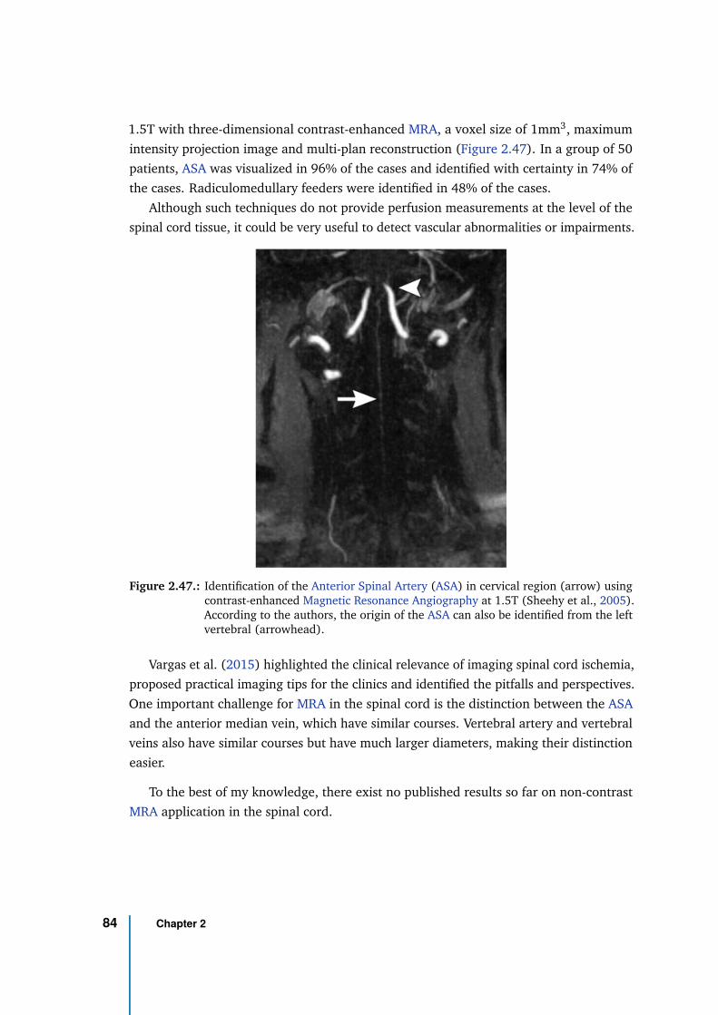
1.5T with three-dimensional contrast-enhanced MRA, a voxel size of 1mm3, maximum

intensity projection image and multi-plan reconstruction (Figure 2.47). In a group of 50

patients, ASA was visualized in 96% of the cases and identified with certainty in 74% of

the cases. Radiculomedullary feeders were identified in 48% of the cases.

Although such techniques do not provide perfusion measurements at the level of the

spinal cord tissue, it could be very useful to detect vascular abnormalities or impairments.

Figure 2.47.: Identification of the Anterior Spinal Artery (ASA) in cervical region (arrow) usingcontrast-enhanced Magnetic Resonance Angiography at 1.5T (Sheehy et al., 2005).According to the authors, the origin of the ASA can also be identified from the leftvertebral (arrowhead).

Vargas et al. (2015) highlighted the clinical relevance of imaging spinal cord ischemia,

proposed practical imaging tips for the clinics and identified the pitfalls and perspectives.

One important challenge for MRA in the spinal cord is the distinction between the ASA

and the anterior median vein, which have similar courses. Vertebral artery and vertebral

veins also have similar courses but have much larger diameters, making their distinction

easier.

To the best of my knowledge, there exist no published results so far on non-contrast

MRA application in the spinal cord.

84 Chapter 2

Altogether, those works attest to the remaining challenges to achieve a reliable

characterization of the spinal cord vascularization and perfusion in humans, which could

be beneficial in the context of Degenerative Cervical Myelopathy (DCM).

2.5 Degenerative Cervical Myelopathy

After traumatic spinal cord injury, Degenerative Cervical Myelopathy (DCM) is proba-

bly an area where spinal cord perfusion MR imaging would be greatly beneficial.

2.5.1 Pathogenesis

Anatomical degenerations

The name Degenerative Cervical Myelopathy (DCM) has been introduced recently by

Nouri et al. (2015) to refer to any degeneration of the cervical spine with alteration over

time, resulting in cervical canal stenosis and eventually symptoms such as pain, motor

and/or sensory disability, diagnosed as cervical myelopathy. This general term was intro-

duced with the objective to pool the different origins of cervical degenerations leading to

myelopathy, which can occur concomitantly but have been diagnosed or identified indi-

vidually as different conditions. The lack of dedicated term and international guidelines

has given rise to ambiguity in exploration and diagnosis of such condition, which can

indeed involve several processes. This lack of consensus might also be responsible for the

sparsity of epidemiological data regarding this pathology.

According to the conceptual classification from Nouri et al. (2015) Figure 2.48,

excluding congenital origins, the two main types of conditions are those induced by

ostheoartritic degenerations (e.g., osteophyte), most common from middle age onward

— Cervical Sondylothic Myelopathy (CSM) is one example —, and the conditions in-

volving non-osteoarthritic processes such as ligament hypertrophy or ossification — e.g.,

Ossification of the Posterior Longitudinal Ligament (OPLL). Those processes often occur

concomitantly.

Such classification is very helpful to further characterize the pathology and its patho-

genesis. The main anatomical degenerations that can be found in DCM patients are

depicted in Figure 2.49. The main degenerating anatomical entities are the vertebrae

2.5 Degenerative Cervical Myelopathy 85

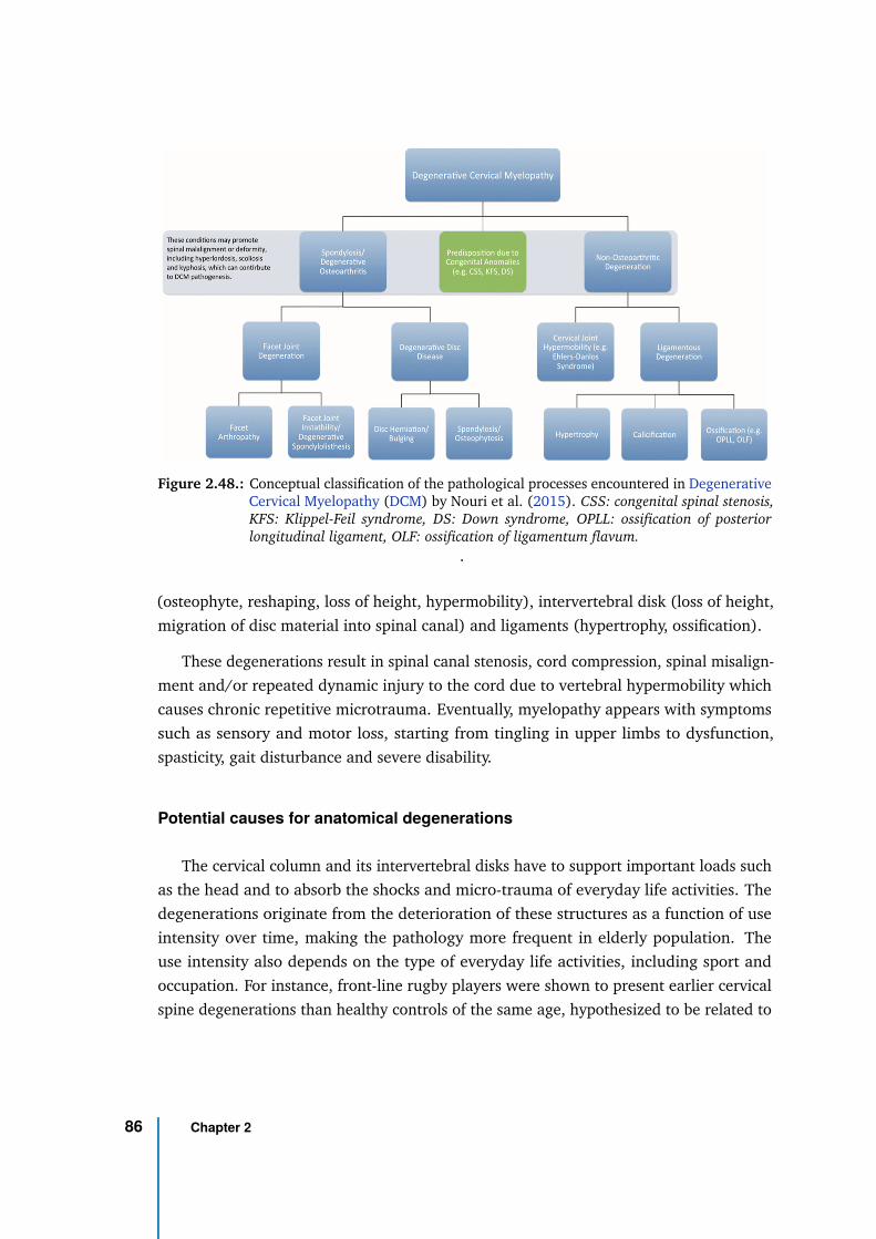
Figure 2.48.: Conceptual classification of the pathological processes encountered in DegenerativeCervical Myelopathy (DCM) by Nouri et al. (2015). CSS: congenital spinal stenosis,KFS: Klippel-Feil syndrome, DS: Down syndrome, OPLL: ossification of posteriorlongitudinal ligament, OLF: ossification of ligamentum flavum.

.

(osteophyte, reshaping, loss of height, hypermobility), intervertebral disk (loss of height,

migration of disc material into spinal canal) and ligaments (hypertrophy, ossification).

These degenerations result in spinal canal stenosis, cord compression, spinal misalign-

ment and/or repeated dynamic injury to the cord due to vertebral hypermobility which

causes chronic repetitive microtrauma. Eventually, myelopathy appears with symptoms

such as sensory and motor loss, starting from tingling in upper limbs to dysfunction,

spasticity, gait disturbance and severe disability.

Potential causes for anatomical degenerations

The cervical column and its intervertebral disks have to support important loads such

as the head and to absorb the shocks and micro-trauma of everyday life activities. The

degenerations originate from the deterioration of these structures as a function of use

intensity over time, making the pathology more frequent in elderly population. The

use intensity also depends on the type of everyday life activities, including sport and

occupation. For instance, front-line rugby players were shown to present earlier cervical

spine degenerations than healthy controls of the same age, hypothesized to be related to

86 Chapter 2

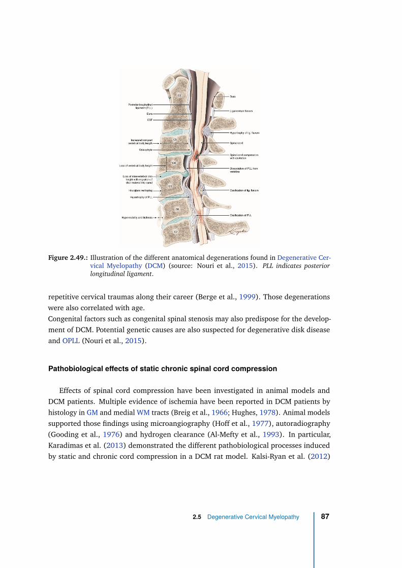
Figure 2.49.: Illustration of the different anatomical degenerations found in Degenerative Cer-vical Myelopathy (DCM) (source: Nouri et al., 2015). PLL indicates posteriorlongitudinal ligament.

repetitive cervical traumas along their career (Berge et al., 1999). Those degenerations

were also correlated with age.

Congenital factors such as congenital spinal stenosis may also predispose for the develop-

ment of DCM. Potential genetic causes are also suspected for degenerative disk disease

and OPLL (Nouri et al., 2015).

Pathobiological effects of static chronic spinal cord compression

Effects of spinal cord compression have been investigated in animal models and

DCM patients. Multiple evidence of ischemia have been reported in DCM patients by

histology in GM and medial WM tracts (Breig et al., 1966; Hughes, 1978). Animal models

supported those findings using microangiography (Hoff et al., 1977), autoradiography

(Gooding et al., 1976) and hydrogen clearance (Al-Mefty et al., 1993). In particular,

Karadimas et al. (2013) demonstrated the different pathobiological processes induced

by static and chronic cord compression in a DCM rat model. Kalsi-Ryan et al. (2012)


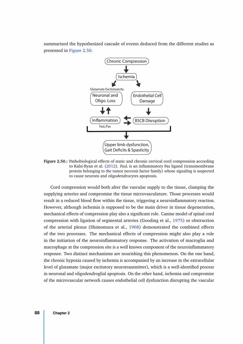
summarized the hypothesized cascade of events deduced from the different studies as

presented in Figure 2.50.

Figure 2.50.: Pathobiological effects of static and chronic cervical cord compression accordingto Kalsi-Ryan et al. (2012). FasL is an inflammatory Fas ligand (transmembraneprotein belonging to the tumor necrosis factor family) whose signaling is suspectedto cause neurons and oligodendrocytes apoptosis.

Cord compression would both alter the vascular supply to the tissue, clamping the

supplying arteries and compromise the tissue microvasculature. Those processes would

result in a reduced blood flow within the tissue, triggering a neuroinflammatory reaction.

However, although ischemia is supposed to be the main driver in tissue degeneration,

mechanical effects of compression play also a significant role. Canine model of spinal cord

compression with ligation of segmental arteries (Gooding et al., 1975) or obstruction

of the arterial plexus (Shimomura et al., 1968) demonstrated the combined effects

of the two processes. The mechanical effects of compression might also play a role

in the initiation of the neuroinflammatory response. The activation of macroglia and

macrophage at the compression site is a well known component of the neuroinflammatory

response. Two distinct mechanisms are nourishing this phenomenon. On the one hand,

the chronic hypoxia caused by ischemia is accompanied by an increase in the extracellular

level of glutamate (major excitatory neurotransmitter), which is a well-identified process

in neuronal and oligodendroglial apoptosis. On the other hand, ischemia and compromise

of the microvascular network causes endothelial cell dysfunction disrupting the vascular

88 Chapter 2

basement membrane and the Blood-Spinal Cord Barrier (BSCB). Disruption of the BSCB

has been reported both in the early and late stages of the compression in DCM (Karadimas

et al., 2013). The infiltration of immune cell through the impaired BSCB exacerbates the

neuroinflammation. A vicious circle is established with inflammation potentiating the

endothelial cell loss and BSCB impairment, which in turn, lets immune cells extravasate

in the tissue environment nourishing the inflammation. Eventually, tumor necrosis

factors (Fas ligands, tumor necrosis factor-α) coming with the neuroinflammation to

regulate the immune system response are though to be responsible for additional neuronal

and oligodendrocytes death. Oligodendrocytes death results in demyelination, axonal

degeneration and axonal loss. Neuronal apoptosis induces an abnormal increase in

the number of astrocytes (astrogliosis), which inhibits axon regeneration, giving way to

myelopathy (Kalsi-Ryan et al., 2012; Nouri et al., 2015).

The inflammatory response in the central nervous system is originally dedicated to

heal the tissue (healing effect). However, as previously mention, it is also responsible for

the exacerbation of the initiated neuronal, oligodendroglial and endothelial cell death

(injurious effect). If at first the inflammatory profile of DCM was thought to be similar to

spinal traumatic injury, it is now becoming apparent that DCM inflammatory profile is slow,

driven by the chronic progressive compression and including compensatory mechanisms

along the compression course (Karadimas et al., 2015). Moreover, compared to spinal

cord injury, DCM does not show hemorrhagic necrosis (tissue death caused by bleeding)

and no evidence of bleeding were reported. However, more insights into the nature of the

inflammatory response to chronic spinal cord compression is needed to understand which

mechanisms are beneficial and which mechanisms are detrimental to the neuronal tissue

degeneration in DCM patients. The temporal profile of the mechanisms also remains

poorly described.

Dynamic injury mechanisms

In addition to static compression, it is recognized that spinal cord is injured by

repetitive dynamic effects with neck motion or vertebral segments hypermobility or

misalignment during everyday life activities. Hayashi et al. (2014) reported that, in a

group of symptomatic patients, anatomical MRI in neutral position showed spinal cord

compression for 5.3% of cases but that MRI examination in extension and flexion position

revealed a missed compression in 8.6% and 1.6% of cases, respectively. Furthermore,

Matsunaga et al. (2002) showed that for patients with spinal canal diameter between 6


and 14 mm, myelopathy preferentially developed in those with increased range of motion,

supposedly because of the dynamic factors.

In light of those results, myelopathy development in DCM cannot be considered solely

due to static chronic spinal cord compression.

Spatial distribution of tissue degenerations

A large proportion of DCM patients shows degenerations at multiple levels at the

same time. The type of degenerations can also be different across levels. According

to Northover et al. (2012), around 80% of patients show a multi-level disease. The

vertebral level the most frequently affected in DCM is C5-C6 (Northover et al., 2012;

Edwards et al., 1983). It could be explained by the higher mobility of the segment in

addition to the small anteroposterior spinal canal diameter at that level (one of the two

segments with the smallest spinal canal diameter) compared to others (Ogino et al.,

1983). Unfortunately, C5 to C7 is also the region with the most vulnerable vascular supply

(Baron et al., 2007; Firooznia et al., 1985; Yue et al., 2001). Nevertheless, the most

frequently affected level is likely to depend on the type of degeneration. For instance,

degenerative spondylolisthesis (translational displacement of one vertebral body over

another) has shown a higher frequency at C3-C4 (46%) and C4-C5 (49%) (Jiang et al.,

2011).

According to Breig et al. (1966), the anterior white matter columns are globally

preserved during anteroposterior compression. As the anterior artery, which directly

supplies those regions, has a zigzag course, the spinal cord inferior-superior stretching

with compression might not distort it significantly, allowing those regions to be irrigated.

In contrast, the infarction of central gray matter observed in DCM patients (Fehlings et al.,

1998; Ogino et al., 1983) could be explained by the obstruction of the central sulcal artery

running along the anteroposterior axis during compression and which is the main supply

to central gray matter. Similarly, corticospinal tracts and posterolateral white matter

seem to be the first and mains region affected by demyelination (Ogino et al., 1983; Breig

et al., 1966). Given that lateral white matter is mainly irrigated by radiculo-medullary

arteries running on the subpial surface with an anteroposterior course when arriving to

lateral white matter, a similar explanation as for gray matter and central sulcal artery can

be made: those arteries are likely to be more vulnerable to anteroposterior compression

(Gooding et al., 1975).

90 Chapter 2

Compensatory mechanisms in the chronically compressed spinal cord

Unlike in traumatic spinal cord injuries, compensatory mechanisms to adapt to the

slow and progressive chronic spinal cord compression occuring in DCM are largely sus-

pected. Several studies have investigated the potential repair and plasticity mechanisms

taking place and that can be used as treatment. Among them, the neurotrophic factors

(proteins involved in neuronal regulation, axonal growth and synaptic plasticity), which

have been used to foster axonal regeneration in injured central nervous system, and their

receptors have shown a higher expression rostrally and caudally to the compression sites

in mouse model compared to uncompresssed sites (Uchida et al., 2003). These results

are consistent with the higher number of neurons and oligodendrocytes reported rostrally

and caudally to the compression sites (Yu et al., 2009). Similarly, the degree of expression

of the growth-associated protein 43 (protein involved in neuronal development and

axonal regeneration) has been related to the degree of injury in a rat model of acute

compression (Li et al., 1996). Those findings are also consistent with correlation between

the increase in immunoreactivity of this protein and the degree and period of compression

reported by in mice (Uchida et al., 2002). Those results suggest that neuronal and axonal

regeneration may occur in the cervical human spinal cord to adapt and compensate for

the slow progression of the compression. Whether these compensatory mechanisms might

be too low or too slow compared to the degeneration, or whether they may end past a

given compression threshold, those are still pending questions.

2.5.2 Diagnosis

Clinical, neurological and radiological presentation

DCM is diagnosed based on clinical symptoms, neurological signs of spinal cord

dysfunction and radiological presentation. Clinical symptoms and neurological signs

must be accompanied with an MRI showing cord compression for DCM to be diagnosed.

Most commonly, the first symptom of DCM would be spastic gait (Gorter, 1976; Lunsford,

1980), followed temporally by upper extremity numbness and loss of fine motor control

of the hands. However, great variations of symptomatic presentation exist across patients,

hence the difficulty to detect DCM in the early stages (Tetreault et al., 2015). Naturally,

patients seek for medical examination when symptoms already appeared. Consequently,

little is known on the relation between the duration of cord compression before the


apparition of symptoms. Symptoms can even appear without static cord compression

visible during radiological examination in neutral position, due to the dynamic injury

component of DCM as previously mentioned.

The main clinical symptoms are (Kalsi-Ryan et al., 2012):

• Numb hands

• Bilateral arm parasthesia

• Spastic Ataxic gait

• L’Hermitte’s phenomenon

• Weakness

The main neurological signs are:

• Corticospinal tract signs

• Hyperreflexia

• Positive Hoffman sign

• Ataxia

• Atrophy of hand muscles

• Spasticity/clonus

And the MRI indicators are:

• Full effacement of CSF and deformation of cord

• Signal change on T1-weighted or T2-weighted image

• Vertebral segment-related signal change on T2-weighted image

• Reduction in cord cross-sectional area

92 Chapter 2

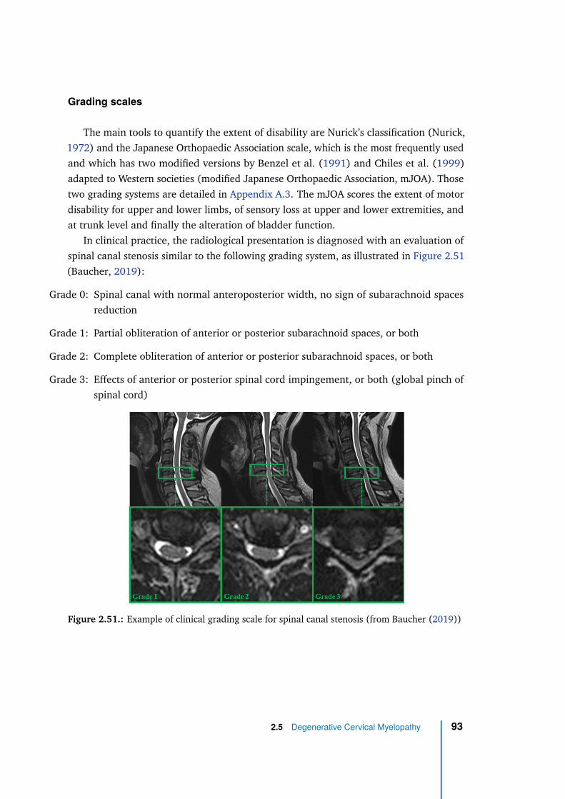
Grading scales

The main tools to quantify the extent of disability are Nurick’s classification (Nurick,

1972) and the Japanese Orthopaedic Association scale, which is the most frequently used

and which has two modified versions by Benzel et al. (1991) and Chiles et al. (1999)

adapted to Western societies (modified Japanese Orthopaedic Association, mJOA). Those

two grading systems are detailed in Appendix A.3. The mJOA scores the extent of motor

disability for upper and lower limbs, of sensory loss at upper and lower extremities, and

at trunk level and finally the alteration of bladder function.

In clinical practice, the radiological presentation is diagnosed with an evaluation of

spinal canal stenosis similar to the following grading system, as illustrated in Figure 2.51

(Baucher, 2019):

Grade 0: Spinal canal with normal anteroposterior width, no sign of subarachnoid spaces

reduction

Grade 1: Partial obliteration of anterior or posterior subarachnoid spaces, or both

Grade 2: Complete obliteration of anterior or posterior subarachnoid spaces, or both

Grade 3: Effects of anterior or posterior spinal cord impingement, or both (global pinch of

spinal cord)

Figure 2.51.: Example of clinical grading scale for spinal canal stenosis (from Baucher (2019))


2.5.3 Treatment

Treatment of DCM depends on the severity of the disease which can be evaluated with

several clinical grading scales such as those mentioned earlier. Usually, a decompressive

surgery is prescribed for moderate to severe DCM cases in order to reduce or even

eliminate the spinal canal stenosis and release the cord from the constraints that apply.

Such surgery is done either from anterior or posterior way. The anterior approach,

preferred for single-level presentations, typically consists of either a discectomy (removal

of the intervertebral disk) or a corpectomy (removal of part of the vertebral body)

(Tannous et al., 2014). The two successive vertebrae are then merged together. In the

posterior approach, most commonly prescribed for multi-level presentations, the vertebral

posterior part is removed (laminectomy) at the different levels involved (Kiely et al.,

2015).

For mild DCM presentations, as the evolution speed of degenerations is relatively

unknown and might vary across individuals, conservative management is preferred

although the number of surgery for mild cases has increased (Fehlings et al., 2017). In

that case, several neuroprotective drugs can potentially regulate inflammation and/or

preserve the tissue neuronal and axonal degeneration. Among them, the riluzole, which

is the only Food and Drug Administration approved pharmacotherapy for amyotrophic

lateral sclerosis, has been used to block glutamate receptors and increase glutamate

transporter activity with the objective to reduce glutamate excitotoxicity induced by

ischemia. It has shown promising results in animal models (Karadimas et al., 2012). Its

neuroprotective benefits to neurological recovery post-surgery are currently appraised in

a clinical trial (Fehlings et al. (2013), https://clinicaltrials.gov/ct2/show/study/

NCT01257828).

2.5.4 Epidemiology

Incidence and prevalence

Degenerative Cervical Myelopathy is the most common progressive non-traumatic

disorder of the spinal cord in the elderly population. However, as previously explained,

its global epidemiology is difficult to estimate because this pathology includes different

degenerative mechanisms which have generally been diagnosed independently. Besides,

most epidemiological studies were carried out in the local country. A comprehensive

94 Chapter 2

https://clinicaltrials.gov/ct2/show/study/NCT01257828

https://clinicaltrials.gov/ct2/show/study/NCT01257828

listing of those studies with the regional incidences of each degenerative type can be

found in Nouri et al. (2015) (see Table 3).

One way to estimate DCM epidemiology is to look at epidemiological data of non-

traumatic spinal cord injuries as they are mostly DCM (beside motor neuron, infectious,

inflammatory, and neoplastic diseases and other). From the data published in New et al.

(2014), the incidence (rate of occurrence of new cases) and the prevalence (proportion of

cases in the population) in North America can be estimated at 41 new cases/million people

and 605 cases/million people, respectively. However, those data might be underestimated

as they are likely to arise from severe DCM cases.

Furthermore, based on the Japanese study of Matsumoto et al. (1998), 88% of the

population (86% of men, 89% of women) above 60 years old would have one or more

severely degenerated cervical level (Matsumoto et al., 1998), representing the population

at risk. For men and women in their 20s, this proportion was reduced to 17% and 12%,

respectively.

Progression rate

An idea of DCM progression rate can be estimated from the longitudinal study of

Wilder et al. (2011) on cervical spine osteoarthritis. The progression rate was defined

based on the grading of radiographic (X-ray) measurements acquired biennially. It

appears that the pathology progresses faster in men than in women at all ages. The

fastest progression would be 12.5 new cases/100 patients/year for men between 70 and

79 years old, and 9.3 new cases/100 patients/year for women older than 80 years old.

According to the systematic review of Wilson et al. (2013), patients with cervical canal

stenosis and cord compression due to spondylosis, without clinical sign of myelopathy,

will develop myelopathy after one year follow-up in 8% of cases and after 44 months in

23% of cases.

Hospitalization rate

The number of hospitalizations for DCM seems to have increased. According to

Lad et al. (2009) regarding Cervical Spondylotic Myelopathy (CSM), it would have

more than doubled between 1992 and 2002 (from 3.73 patients/100,000 people to

7.88) in the United States. The number of vertebral fusions would also have increased

and been multiplied by 7 (from 0.6 patients/100,000 people to 4.1). However, this


might be attributable to the evolution of the understanding of DCM as a pathology

not only induced by static cord compression but also by dynamic injuries and vertebral

misalignment. According to Oglesby et al. (2013), from 2002 to 2009, the number of

cervical procedures in the United States increased from 150,327 (52.2/100,000 people)

to 186,679 (60.8/100,000 people). Finally, based on a systematic review of the literature

between 2012 and 2015 (Tetreault et al., 2017), the incidence rate of hospitalization for

spinal cord injury in CSM patients was 13.9/1,000 person-years and 4.8/1,000 person-

years for patients with DCM from OPLL. The hospitalization rate for spinal cord injury

in patients with DCM from OPLLwas significantly higher than in a healthy population

(0.18/1,000 person-years).

Survival

From a study on non-traumatic spinal cord injuries in Israel (Ronen et al., 2004), the

survival duration of patients with non-traumatic injury at cervical level would be 22.7

years whereas it would be of 17.6 years for patients with spinal stenosis only (but at

any spine level). The survival of patients with non-traumatic spinal cord injury due to

herniated disk would be 29 years but those were mainly at the lumbar level.

2.5.5 Application of electrophysiology in DCM

Electrophysiology consists in measuring voltage changes or electric currents, related

to neuronal activity in the case of neurologic applications. It is an important tool used for

diagnosis in clinics to help localizing lesions (e.g., can tell whether lesion is in gray matter

anterior horn or in corticospinal tract) and objectively detect spinal cord dysfunction

(Dvorak et al., 2005). In cervical spinal cord, the most common eletrophysiological tests

are Somatosensory Evoked Potential (SEP) and Motor Evoked Potential (MEP) (Zileli

et al., 2019). SEP is used to assess the dorsal column. Typically, surface electrodes

are placed on the scalp of the patient overlying the primary sensory area, or at lumbar

or cervical spine level. Electrical stimulation of peripheral nerves (e.g., posterior tibial

or peroneal nerves of the lower limbs) or skin (from the contralateral limb) is then

applied and action potentials are recorded. Nerves from different spinal levels need to be

stimulated for diagnosis of the level. SEP is recommended for diagnosis of DCM (Vohanka

et al., 1993). Improvement in SEP in the early decompression period was also shown to

correlate with good outcome surgery at 3 months post-surgery (Morishita et al., 2005).

96 Chapter 2

MEP tests look at the motor function and mainly at the corticospinal tract. Short magnetic

pulses are applied to the scalp of the patient using the Transcranial Magnetic Stimulation

technique and a specific coil (Barker et al., 1985) in such a way as to stimulate the motor

cortex, the cervical and lumbar nerve roots and associated peripheral nerves (Chomiak

et al., 1995). The evoked potentials are then recorded with surface electrodes positioned

on muscles such as abductor or quadriceps. Diagnosis on the affected spinal level(s)

is then performed based on the known innervation of stimulated muscles. The value

of MEP tests for assessment of corticospinal function changes before and after surgery

were evaluated in DCM. A more sensitive recruitment of MEP at 3 months post-surgery

suggested a functional recovery of the corticospinal pathways (Nicotra et al., 2013).

Other electrophysiological tests can be performed in the cervical spinal cord, such as

electromyography (EMG) and nerve conduction study (NCS) (Zileli et al., 2019).

Electrophysiology (SEP and MEP) can therefore provide interesting prognosis predic-

tors and surgical markers in the context DCM.

2.5.6 Application of multi-parametric quantitative MRI in DCM

Combining multiple quantitative MRI techniques to better characterize tissue injury in

DCM patients is an interesting strategy that has been already evaluated in several studies.

It showed a great potential to increase the precision of DCM diagnosis and prognosis, espe-

cially to predict surgery outcome and to better understand the pathology (Zhang, 2014).

For example, Martin et al. (2018) assessed the potential of CSA, Fractional Anisotropy

(FA) from DTI, Magnetization Transfer Ratio (MTR) and T2*-weighted WM/GM ratio for

monitoring myelopathic progression in 26 DCM patients. Quantitative MRI showed 100%

sensitivity and 53.3% specificity while mJOA and conventional T1- and T2-weighted

MRI yielded 25.3% and 18.2% sensitivity and 100% and 81.3% specificity, respectively.

Grabher et al. (2016) were able to show regional atrophy and microstructural damage in

DCM patients far above the stenosis at a level not directly affected by the compression,

using CSA and DTI. Regarding metabolism alteration, Holly et al. (2009) measured a

significantly reduced ratio of N-acetylaspartate (NAA)/Creatine (Cr) concentration in

DCM patients compared to healthy controls using Magnetic Resonance Spectroscopy

(MRS), but this ratio was not correlated with the severity of the myelopathy. Interest-

ingly, Ellingson et al. (2015) combined Diffusion Tensor Imaging and MRS to define a

biomarker based on DTI fiber density, mean diffusivity and concentration ratio Choline

(Cho)/NAA, which showed a significant prediction of the mJOA (R2=0.8) in 27 DCM


patients. Functional MRI (fMRI) in brain has also been applied to DCM, in particular

to study the outcome of decompression surgery and functional recovery of the patient.

Differences in volume of activation were found pre-decompression surgery with respect

to healthy controls, post-decompression surgery with respect to controls and pre- and

post-surgery, suggesting a reorganization of the cortex in DCM patients (Duggal et al.,

2010). An alteration of the resting-state spontaneous activity of cortical neurons within

the sensorimotor network was also reported with resting-state fMRI, both before and

after decompression surgery (Tan et al., 2015).

In addition to prognosis issues, important questions regarding pathogenesis of DCM

still remain. In particular, the chain of processes from the spinal cord mechanical

compression leading to the myelopathy (resulting symptoms) and the timings of each

of those processes still needs to be understood and characterized. The relation between

the degree of compression and the resulting damage seems highly variable, with a broad

range of hardly predictable symptoms as per the current knowledge. New insights on

those questions would greatly benefit to the management and prognosis of patients.

2.6 Biomechanical modeling of spinal cord compression

To study the in-vivo mechanics of human pathologies or injuries (“bio-mechanics”),

three approaches are possible. 1) In-vitro mechanical models can be designed with either

synthetic materials or biologic samples harvested from cadavers with the objective to

reproduce the observed mechanisms and measure the effects. 2) The pathology or injury

can be reproduced in animal models and results are then extrapolated to human. Or

finally, 3) numerical models of human can be designed to simulate the pathology or

injury and estimate the effects with numerical calculations. The last approach, referred

as finite element modeling, is the most appropriate to study pathologies which deeply

involve in-vivo processes and anatomical dependencies such as Degenerative Cervical

Myelopathy (DCM).

98 Chapter 2

2.6.1 Finite element modeling

The finite element method

The finite element method is a numerical technique for solving problems which

involve continuous field systems under external influence and which are described

by comprehensive mathematical equations. The problems can be static or dynamic.

They can be exclusively structural (stress analysis), thermal (analysis of temperature

propagation), electromagnetic (analysis of electromagnetic fields propagation) or fluid-

mechanical, or they can combine those disciplines. The equations can include variable

such as displacement or temperature and physical properties such as density, stiffness,

permeability or conductivity.

The finite element method consists in dividing the geometrical model of the object

under study into an assembly of small parts called finite elements. Those elements are

interconnected by nodes and the action of the variable through or over each of them are

governed according to predefined functions (e.g., constant, linear, quadratic). Thanks

to the recent development of numerical calculations, it is possible to assemble those

equations into a global system and solve the problem with proper boundaries conditions.

The main steps of a finite element analysis are the following:

1. Geometrical design of the model. In the context of biomechanics, this step is often

perform based on anatomical images (e.g, CT scan, MRI, electron microscopy

images) of the body part to be studied. A reconstruction in 3D is usually involved.

2. Model discretization or meshing. The geometrical model domain is divided into

discrete or finite elements, making up the mesh. The resolution, number and

types of elements is a critical step. A too coarse mesh can result in an inadequate

parametric distribution whereas a too fine resolution can increase the computing

time needlessly and can even prevent the problem to solve. As more than millions of

elements are to be created, this step can hardly be done manually. Specific software

with automatic meshing methods are used. The description of the mesh is stored in

a big array containing the nodes coordinates and the element connectivities. The

element types (e.g, tetrahedral, hexahedral) are defined during this step too.

3. Definition of the interpolation functions within the elements. Interpolation functions

are necessary to interpolate the field variation over the element. Polynomial

2.6 Biomechanical modeling of spinal cord compression 99

functions are often used, with the degree depending on the number of nodes of the

element.

4. Definition of the element properties. The matrix equation defining how the variable

(e.g., displacement in structural analysis, temperature in thermal analysis) acts

through or over each element has to be established. Such matrix equation relates

the nodal values of the field to the element parameters such as the stiffness and the

density. Different formulations exist. The most popular are the Galerkin method, for

physical problems described by differential equations, and the variational formula-

tion for physical problems well described by a function minimization.

5. Assembly of the individual element equations into a global equation system. For

the example of a linear static analysis, the global equation system takes the form

K.δ = F where K is a the global stiffness matrix (square matrix), δ is the vector of

unknown nodal displacement (or temperature for thermal analysis) and F is the

vector of applied nodal forces (or heat flux in thermal analysis).

6. Definition of loading and boundary conditions. As the problem is to predict the field

variation in the system under external influence, the external influence referred

as loading, needs to be defined (e.g., displacement of an impinger along time).

Moreover, for the equation system to be solved, boundary conditions (e.g., null

displacement (δ = 0) at extremity nodes) need to be set.

7. Global equation system solving. To solve quasi-static problems, two methods exist:

the implicit method, better designed for static problems, and the explicit method

(more effective for dynamic problems) with energy relaxation as used in this PhD

thesis. With the implicit method, we seek to invert the system in order to obtain

the unknown nodal displacement δ = K−1.F according to the same example of

linear static analysis introduced earlier. However, due to the very large number of

equations, the system requires large memory storage and cannot be easily inverted.

Fortunately, the system is sparse, symmetric and positive definite. Direct and

iterative techniques have been developed to take advantage of those features to

store and solve the system efficiently. With the explicit method, the equation

includes acceleration and velocity such as M · δ + C · δ + Kδ = F , with M and C

generally being diagonal matrices easy to invert. For each node, the acceleration

is calculated at time step n as the difference between external and internal nodal

forces over the mass: δn = fext(tn)−fint(tn)m . Then, the velocity for time step n + 1

2

and displacement for time step n + 1 are derived according to: δn+ 1

2

= δn−1

2

+ δn∆t

100 Chapter 2

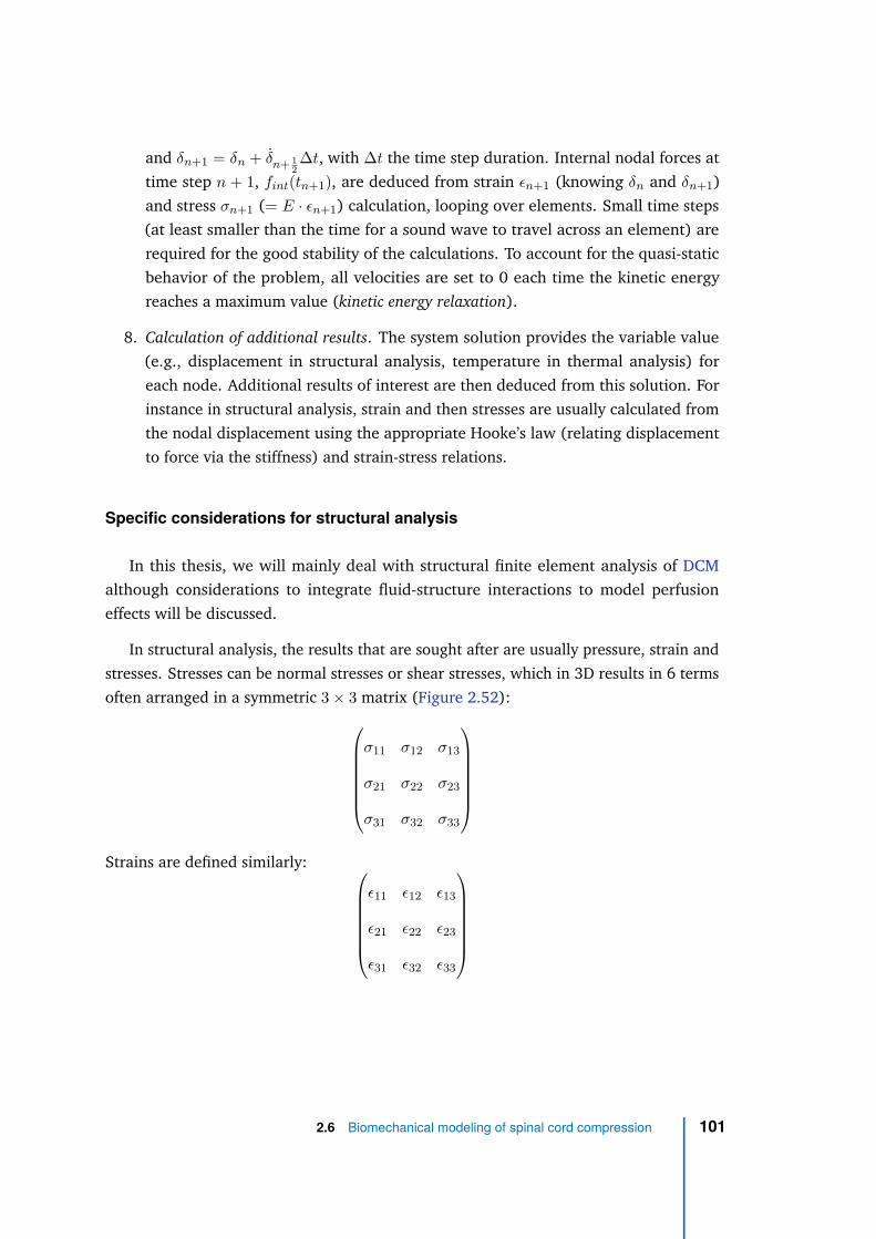
and δn+1 = δn + δn+ 1

2

∆t, with ∆t the time step duration. Internal nodal forces at

time step n + 1, fint(tn+1), are deduced from strain ǫn+1 (knowing δn and δn+1)

and stress σn+1 (= E · ǫn+1) calculation, looping over elements. Small time steps

(at least smaller than the time for a sound wave to travel across an element) are

required for the good stability of the calculations. To account for the quasi-static

behavior of the problem, all velocities are set to 0 each time the kinetic energy

reaches a maximum value (kinetic energy relaxation).

8. Calculation of additional results. The system solution provides the variable value

(e.g., displacement in structural analysis, temperature in thermal analysis) for

each node. Additional results of interest are then deduced from this solution. For

instance in structural analysis, strain and then stresses are usually calculated from

the nodal displacement using the appropriate Hooke’s law (relating displacement

to force via the stiffness) and strain-stress relations.

Specific considerations for structural analysis

In this thesis, we will mainly deal with structural finite element analysis of DCM

although considerations to integrate fluid-structure interactions to model perfusion

effects will be discussed.

In structural analysis, the results that are sought after are usually pressure, strain and

stresses. Stresses can be normal stresses or shear stresses, which in 3D results in 6 terms

often arranged in a symmetric 3 × 3 matrix (Figure 2.52):

σ11 σ12 σ13

σ21 σ22 σ23

σ31 σ32 σ33

Strains are defined similarly:

ǫ11 ǫ12 ǫ13

ǫ21 ǫ22 ǫ23

ǫ31 ǫ32 ǫ33


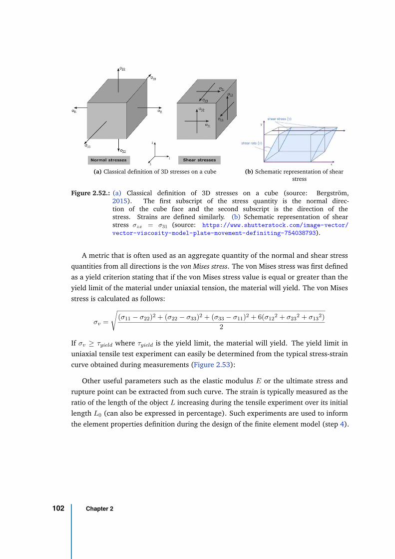
(a) Classical definition of 3D stresses on a cube (b) Schematic representation of shearstress

Figure 2.52.: (a) Classical definition of 3D stresses on a cube (source: Bergström,2015). The first subscript of the stress quantity is the normal direc-tion of the cube face and the second subscript is the direction of thestress. Strains are defined similarly. (b) Schematic representation of shearstress σzx = σ31 (source: https://www.shutterstock.com/image-vector/

vector-viscosity-model-plate-movement-definiting-754038793).

A metric that is often used as an aggregate quantity of the normal and shear stress

quantities from all directions is the von Mises stress. The von Mises stress was first defined

as a yield criterion stating that if the von Mises stress value is equal or greater than the

yield limit of the material under uniaxial tension, the material will yield. The von Mises

stress is calculated as follows:

σv =

√(σ11 − σ22)2 + (σ22 − σ33)2 + (σ33 − σ11)2 + 6(σ12

2 + σ232 + σ13

2)

2

If σv ≥ τyield where τyield is the yield limit, the material will yield. The yield limit in

uniaxial tensile test experiment can easily be determined from the typical stress-strain

curve obtained during measurements (Figure 2.53):

Other useful parameters such as the elastic modulus E or the ultimate stress and

rupture point can be extracted from such curve. The strain is typically measured as the

ratio of the length of the object L increasing during the tensile experiment over its initial

length L0 (can also be expressed in percentage). Such experiments are used to inform

the element properties definition during the design of the finite element model (step 4).

102 Chapter 2

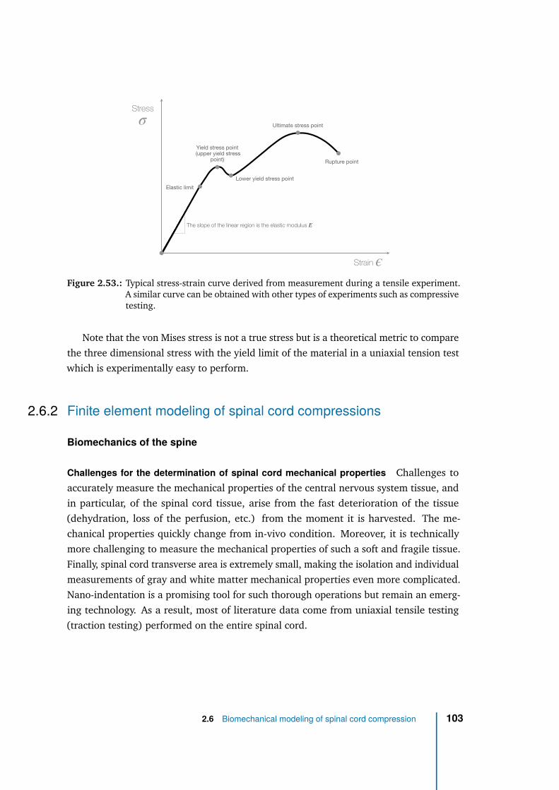
https://www.shutterstock.com/image-vector/vector-viscosity-model-plate-movement-definiting-754038793

https://www.shutterstock.com/image-vector/vector-viscosity-model-plate-movement-definiting-754038793

Stress

Strain

Elastic limit

Yield stress point (upper yield stress

point)

Lower yield stress point

Ultimate stress point

Rupture point

The slope of the linear region is the elastic modulus E

σ

ϵ

Figure 2.53.: Typical stress-strain curve derived from measurement during a tensile experiment.A similar curve can be obtained with other types of experiments such as compressivetesting.

Note that the von Mises stress is not a true stress but is a theoretical metric to compare

the three dimensional stress with the yield limit of the material in a uniaxial tension test

which is experimentally easy to perform.

2.6.2 Finite element modeling of spinal cord compressions

Biomechanics of the spine

Challenges for the determination of spinal cord mechanical properties Challenges to

accurately measure the mechanical properties of the central nervous system tissue, and

in particular, of the spinal cord tissue, arise from the fast deterioration of the tissue

(dehydration, loss of the perfusion, etc.) from the moment it is harvested. The me-

chanical properties quickly change from in-vivo condition. Moreover, it is technically

more challenging to measure the mechanical properties of such a soft and fragile tissue.

Finally, spinal cord transverse area is extremely small, making the isolation and individual

measurements of gray and white matter mechanical properties even more complicated.

Nano-indentation is a promising tool for such thorough operations but remain an emerg-

ing technology. As a result, most of literature data come from uniaxial tensile testing

(traction testing) performed on the entire spinal cord.


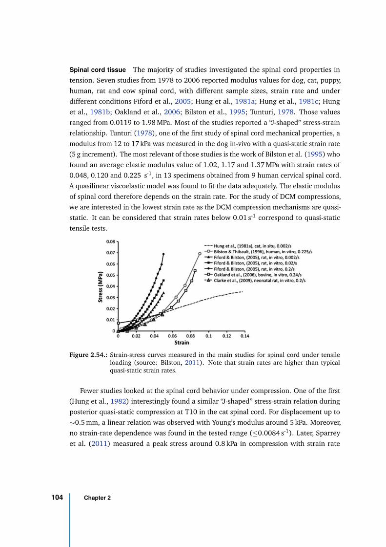
Spinal cord tissue The majority of studies investigated the spinal cord properties in

tension. Seven studies from 1978 to 2006 reported modulus values for dog, cat, puppy,

human, rat and cow spinal cord, with different sample sizes, strain rate and under

different conditions Fiford et al., 2005; Hung et al., 1981a; Hung et al., 1981c; Hung

et al., 1981b; Oakland et al., 2006; Bilston et al., 1995; Tunturi, 1978. Those values

ranged from 0.0119 to 1.98 MPa. Most of the studies reported a “J-shaped” stress-strain

relationship. Tunturi (1978), one of the first study of spinal cord mechanical properties, a

modulus from 12 to 17 kPa was measured in the dog in-vivo with a quasi-static strain rate

(5 g increment). The most relevant of those studies is the work of Bilston et al. (1995) who

found an average elastic modulus value of 1.02, 1.17 and 1.37 MPa with strain rates of

0.048, 0.120 and 0.225 s-1, in 13 specimens obtained from 9 human cervical spinal cord.

A quasilinear viscoelastic model was found to fit the data adequately. The elastic modulus

of spinal cord therefore depends on the strain rate. For the study of DCM compressions,

we are interested in the lowest strain rate as the DCM compression mechanisms are quasi-

static. It can be considered that strain rates below 0.01 s-1 correspond to quasi-static

tensile tests.

Figure 2.54.: Strain-stress curves measured in the main studies for spinal cord under tensileloading (source: Bilston, 2011). Note that strain rates are higher than typicalquasi-static strain rates.

Fewer studies looked at the spinal cord behavior under compression. One of the first

(Hung et al., 1982) interestingly found a similar “J-shaped” stress-strain relation during

posterior quasi-static compression at T10 in the cat spinal cord. For displacement up to

∼0.5 mm, a linear relation was observed with Young’s modulus around 5 kPa. Moreover,

no strain-rate dependence was found in the tested range (≤0.0084 s-1). Later, Sparrey

et al. (2011) measured a peak stress around 0.8 kPa in compression with strain rate

104 Chapter 2

0.005 s-1 in porcine spinal white matter while Jannesar et al. (2018) measured a peak

stress of 7 kPa with strain rate 0.3 s-1 in non-human primate spinal white matter. In

human, the results from Hung et al. (1982) were supported 35 years later by Karimi et al.

(2017) in 24 male cadavers’ spinal cord at cervical level. A global nonlinear hyperelastic

behavior was observed (“J-shaped” stress-strain relation) and constants for Yeoh, Ogden

and Mooney-Rivlin laws were estimated. The linear model was also approximated and

yielded a mean elastic modulus of 40.12 kPa and peak stress of 62.26 kPa for a strain rate

of 1 s-1.

The literature therefore shows a great variability of the values, partly due to the

different loading types (tension, compression), strain rates and species. Nevertheless, it

seems that a hyperelastic model for the spinal cord tissue is adapted both in tension and

compression.

White versus gray matter Because of their difference in composition between white and

gray matter, different mechanical properties are expected between those two tissue types.

So far, four groups looked at those differences in different species. With tensile testing

in the cow, GM was found stiffer than WM with elastic modulus from 64 to 166 kPa

for strain rates from 3 × 10−4 to 5 × 10−2 s-1 in GM compared to 30 to 94 kPa for WM

(Ichihara et al., 2001; Ichihara et al., 2003). In the rabbit, GM was also found stiffer than

WM (3.3 vs. 3.2 kPa) during tensile testing but with a different methodology (pipette

aspiration method) (Ozawa et al., 2001). However the difference was not significant. In

the mouse, this time through indentation testing, Koser et al. (2015) supported those

findings reporting an elastic modulus of 0.127 kPa for GM and 0.067 kPa for WM, with

a strain rate of 2 × 10−2 s-1. Finally, according to the results of Nishida et al. (2020) in

compression, the gray matter would show less plasticity, suggesting a stiffer material than

white matter. The cell population in anterior gray matter horns was shown to decrease

under compression loading starting from a reduction in cord CSA of 30%, and reaching a

plateau from a CSA of 50% (Baba et al., 1996; Baba et al., 1997).

If all those studies agree with a higher modulus and stiffness of GM compared to WM,

the values substantially vary across studies, even for similar strain rates.

Interestingly, Ozawa et al. (2001) (in rabbit with pipette aspiration method) and

Koser et al. (2015) (with indentation method) measured the elastic modulus of the two

tissue types in the different orientation (axial, transversal and sagittal) to estimate the

anisotropy. It appeared that gray matter would behaves like an isotropic material whereas

white matter would be more anisotropic. However, one study found a higher elasstic


modulus of WM in axial and transversal directions (Ozawa et al., 2001) and the other

in the transversal and sagittal directions (Koser et al., 2015), which would be more

consistent with the longitudinal organization of white matter fibers.

Pia and dura mater Mazuchowski et al. (2003) showed the important mechanical role

of the pia mater during axial tensile testing, reducing the elastic modulus of the cord from

1.40 to 0.089 MPa when incising the pia mater. Indeed, the pia mater was shown to have

an elastic modulus of 2300 kPa, which is about 460 times higher than the spinal cord

tissue alone (Ozawa et al., 2004). By covering the spinal cord tissue (or parenchyma),

the pia mater triples the elastic modulus of the spinal cord and has an important function

for the spinal cord to recover its shape after injury. The dura mater, made of collagen

fibers mainly oriented in the longitudinal direction, plays a similar role in protection and

shape support with a stronger tensile strength and stiffness in the longitudinal than in

the circumferential direction (Runza et al., 1999).

Nerve roots In vitro, mouse nerve roots showed an elastic modulus of 1300 kPa under

tensile loading with quasi-static stretch rate (0.01 mm/s) (Singh et al., 2006). In pigs,

elastic modulus was around 2100 kPa (Nishida et al., 2015b). Therefore, nerve roots are

expected to be much stiffer (∼100 times) than spinal cord.

Ligaments The various ligaments of cervical spine showed different mechanical proper-

ties. Yoganandan et al. (2000) fitted a bilinear model to the cervical ligaments stress-strain

measurements, with a first linear region with elastic modulus E1 from strain 0 to ǫ12,

followed by a second linear region with elastic modulus E2. Obtained values were

summarized in Table 2.6.

Those results show that ligaments stiffness is of a very different order of magnitude

(∼1000 higher) compared to spinal cord tissue.

Intervertebral disks The interverbral discs, which play a role of shock absorber and

enables movements between adjacent vertebrae, are made of a fibrous outer layer called

the anulus fibrosus and a gelatinous and highly hydrated (∼85% water) center called

the nucleus pulposus (Figure 2.55). The nucleus pulposus takes 30 to 50% of the disc

transverse area and largely accounts for the elasticity of the disk. Intervertebral disc

106 Chapter 2

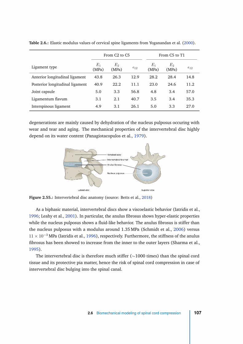
Table 2.6.: Elastic modulus values of cervical spine ligaments from Yoganandan et al. (2000).

From C2 to C5 From C5 to T1

Ligament typeE1

(MPa)E2

(MPa)ǫ12

E1

(MPa)E2

(MPa)ǫ12

Anterior longitudinal ligament 43.8 26.3 12.9 28.2 28.4 14.8

Posterior longitudinal ligament 40.9 22.2 11.1 23.0 24.6 11.2

Joint capsule 5.0 3.3 56.8 4.8 3.4 57.0

Ligamentum flavum 3.1 2.1 40.7 3.5 3.4 35.3

Interspinous ligament 4.9 3.1 26.1 5.0 3.3 27.0

degenerations are mainly caused by dehydration of the nucleus pulposus occuring with

wear and tear and aging. The mechanical properties of the intervertebral disc highly

depend on its water content (Panagiotacopulos et al., 1979).

Figure 2.55.: Intervertebral disc anatomy (source: Betts et al., 2018)

As a biphasic material, intervertebral discs show a viscoelastic behavior (Iatridis et al.,

1996; Leahy et al., 2001). In particular, the anulus fibrosus shows hyper-elastic properties

while the nucleus pulposus shows a fluid-like behavior. The anulus fibrosus is stiffer than

the nucleus pulposus with a modulus around 1.35 MPa (Schmidt et al., 2006) versus

11 × 10−3 MPa (Iatridis et al., 1996), respectively. Furthermore, the stiffness of the anulus

fibrosus has been showed to increase from the inner to the outer layers (Sharma et al.,

1995).

The intervertebral disc is therefore much stiffer (∼1000 times) than the spinal cord

tissue and its protective pia matter, hence the risk of spinal cord compression in case of

intervertebral disc bulging into the spinal canal.


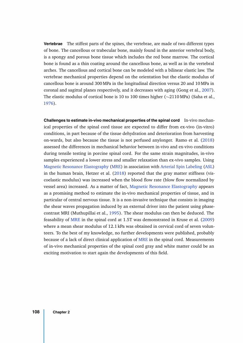
Vertebrae The stiffest parts of the spines, the vertebrae, are made of two different types

of bone. The cancellous or trabecular bone, mainly found in the anterior vertebral body,

is a spongy and porous bone tissue which includes the red bone marrow. The cortical

bone is found as a thin coating around the cancellous bone, as well as in the vertebral

arches. The cancellous and cortical bone can be modeled with a bilinear elastic law. The

vertebrae mechanical properties depend on the orientation but the elastic modulus of

cancellous bone is around 300 MPa in the longitudinal direction versus 20 and 10 MPa in

coronal and sagittal planes respectively, and it decreases with aging (Gong et al., 2007).

The elastic modulus of cortical bone is 10 to 100 times higher (∼2110 MPa) (Saha et al.,

1976).

Challenges to estimate in-vivo mechanical properties of the spinal cord In-vivo mechan-

ical properties of the spinal cord tissue are expected to differ from ex-vivo (in-vitro)

conditions, in part because of the tissue dehydration and deterioration from harvesting

on-wards, but also because the tissue is not perfused anylonger. Ramo et al. (2018)

assessed the differences in mechanical behavior between in-vivo and ex-vivo conditions

during tensile testing in porcine spinal cord. For the same strain magnitudes, in-vivo

samples experienced a lower stress and smaller relaxation than ex-vivo samples. Using

Magnetic Resonance Elastography (MRE) in association with Arterial Spin Labeling (ASL)

in the human brain, Hetzer et al. (2018) reported that the gray matter stiffness (vis-

coelastic modulus) was increased when the blood flow rate (blow flow normalized by

vessel area) increased. As a matter of fact, Magnetic Resonance Elastography appears

as a promising method to estimate the in-vivo mechanical properties of tissue, and in

particular of central nervous tissue. It is a non-invasive technique that consists in imaging

the shear waves propagation induced by an external driver into the patient using phase-

contrast MRI (Muthupillai et al., 1995). The shear modulus can then be deduced. The

feasability of MRE in the spinal cord at 1.5T was demonstrated in Kruse et al. (2009)

where a mean shear modulus of 12.1 kPa was obtained in cervical cord of seven volun-

teers. To the best of my knowledge, no further developments were published, probably

because of a lack of direct clinical application of MRE in the spinal cord. Measurements

of in-vivo mechanical properties of the spinal cord gray and white matter could be an

exciting motivation to start again the developments of this field.

108 Chapter 2

Finite element modeling of spinal cord compressions occurring in Degenerative

Cervical Myelopathy

Spine models for traumatic spinal cord injuries Several finite element models of the

spine were designed to simulate and study traumatic spinal cord injuries such as hap-

pening during traffic accident (Scifert et al., 2002; Greaves et al., 2008; Li et al., 2009;

Wilcox et al., 2003; Wilcox et al., 2004; Czyz et al., 2011; Khuyagbaatar et al., 2014).

Occurring in few seconds, they involve a different dynamic than injuries secondary to

chronic spinal cord compressions which extend over several years. Those models did not

differentiate the spinal cord tissue between white and gray matter.

From simplistic spheres to spinal cord models distinguishing gray and white matter The

first to study DCM pathogenesis with biomechanical numerical simulations was Levine

(1997). The spinal cord model consisted in a simple sphere without distinction between

white and gray matter.

The first model to make a distinction between white and gray matter was proposed by

Ichihara et al. (2001) who compared the behavior of in-vitro compression experiments on

bovine spinal cord to the response of a 2D finite element model mimicking the experiment

and integrating tensile measurements of the properties of the two tissue type. The model

also included the pia mater. Simulations concurred with experimental results. Two

years later, Ichihara et al. (2003) proposed a finer analysis of chronic and dynamic cord

compression with three models: (A) global dynamic anterior compression (1 mm/s), (B)

global static anterior compression (0 mm/s) and (C) global static anterior compression

in association with a dynamic posterior compression by two semi-spheres. Those three

models are interesting to differentiate the effects of static compression from dynamic

effects, as well global versus acute compressions. Based on those results, the authors

suggested that traumatic spinal cord injuries were similar to DCM pathological processes.

The larger damages observed in posterolateral white matter with model (C) are related to

corticospinal tracts degenerations observed in DCM. An interesting point deduced from

model (B) is that, during static compression, the stress relaxation within the spinal cord

measured in-vitro maintains a low intra-cord stress, allowing a sustainable blood flow,

explaining the absence of occluded vessels in the spinal cord parenchyma.

Another study from the same group looked at the effects of anterior neck flexion on

spinal cord under preliminary semi-static compression (Kato et al., 2008). A 5° flexion

was shown to increase stress, especially in anterior and posterior gray matter horns. After


a 10° flexion stress was also observed and posterior and part of lateral white matter.

Although modeling only a slice of the spinal cord with a large anterior compressive bar,

this 6-layer 3D finite element model featured pia mater, white and gray matter, plus a

posterior constraint to simulate dura mater.

Sparrey et al. (2009) proposed a 3D finite element model built out of a published

MRI scan of human thoracic spinal cord to study the effects of tissue property changes

on outcome of posterior compression. An implicit solver was used. Changes in resulting

principal stress, strain, shear stress, shear strain and pressure were quantified. Up to 244%

change in principal stress was measured due to material (tangent modulus) variation.

Strains were less sensitive. Pia mater properties showed little effects. In contrast, white

matter properties had important effect on pressure values both in gray and white matter

which has been related to tissue perfusion (Carlson et al., 1997; Carlson et al., 2000).

The authors conclude that tissue degenerations with aging or disease would affect the

mechanics of spinal cord compression. Still, compression was modeled by a posterior

compressive bar against an anterior compressive bar.

With a similar model as in Kato et al. (2008), Kato et al. (2010) studied the stress

increase within the spinal cord as a function of the antero-posterior compression degree.

The authors concluded that the critical point when stress magnitude may contribute to

myelopathy would be between 20 % and 40 % compression.

Effect of the angle of the anterior compression induced by Ossification of the Posterior

Longitudinal Ligament (OPLL) (“local ossification angle”) was also investigated along

with simulations of decompression and kyphosis conditions (Nishida et al., 2011). Results

suggested that an angle greater than 20° could be detrimental at the thoracic level and

would required additional decompression or kyphosis correction.

Towards DCM-specific designs Nishida et al. (2012) was the first finite element study to

distinguish different types of anterior compression. Three types of anterior compression

were simulated (central, lateral and diffuse or global) along with a fixed angled plate

modeling the restrictions from the ligamentum flavum on the posterior side of the cord. In

addition, a 20° flexion of the cord (as if the head was moved backward during an extension

of the neck) was applied. Results showed higher stress for the diffuse compression type.

Invagination of the ligamentum flavum also induced different stress distributions. Also

looking at the effects of OPLL and of the ligamentum flavum, Kim et al. (2013) proposed

a 3D finite element model made out of a sagittal MRI scan at the thoracolumbar level

of a 75-year old man, distinguishing gray and white matter. Several impinger shapes

(individual simulations for each ligament) and compression degrees (based on the cord

110 Chapter 2

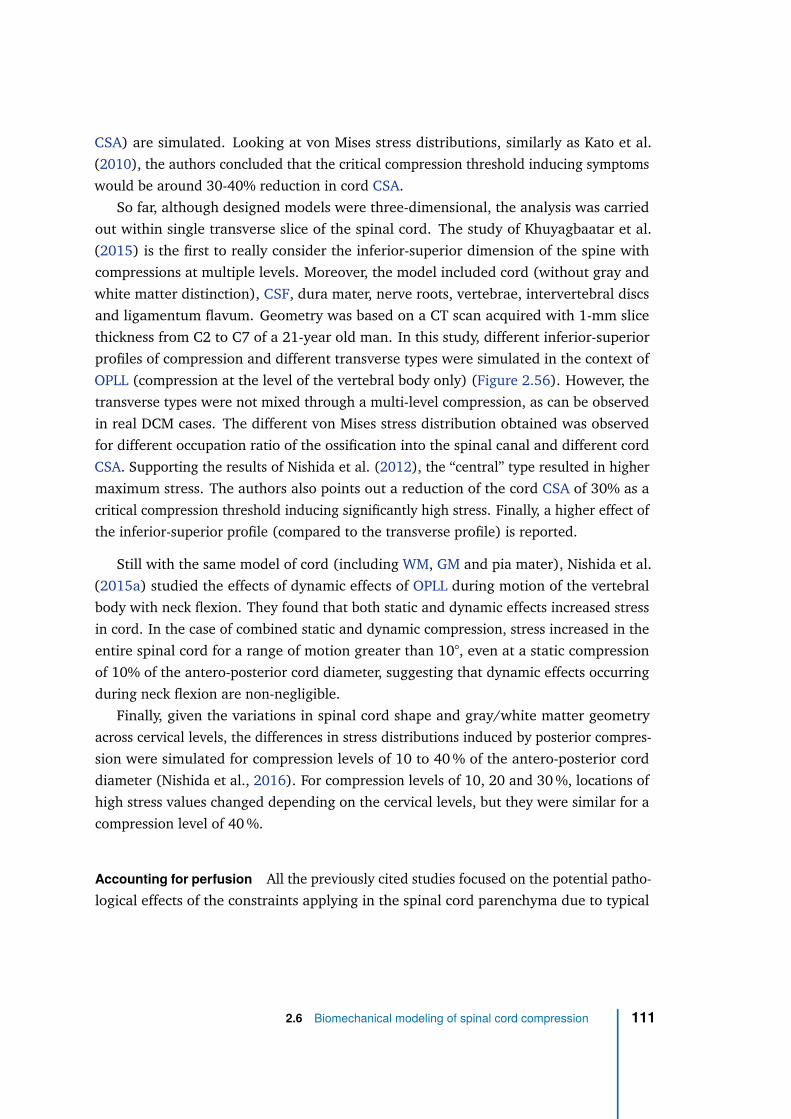
CSA) are simulated. Looking at von Mises stress distributions, similarly as Kato et al.

(2010), the authors concluded that the critical compression threshold inducing symptoms

would be around 30-40% reduction in cord CSA.

So far, although designed models were three-dimensional, the analysis was carried

out within single transverse slice of the spinal cord. The study of Khuyagbaatar et al.

(2015) is the first to really consider the inferior-superior dimension of the spine with

compressions at multiple levels. Moreover, the model included cord (without gray and

white matter distinction), CSF, dura mater, nerve roots, vertebrae, intervertebral discs

and ligamentum flavum. Geometry was based on a CT scan acquired with 1-mm slice

thickness from C2 to C7 of a 21-year old man. In this study, different inferior-superior

profiles of compression and different transverse types were simulated in the context of

OPLL (compression at the level of the vertebral body only) (Figure 2.56). However, the

transverse types were not mixed through a multi-level compression, as can be observed

in real DCM cases. The different von Mises stress distribution obtained was observed

for different occupation ratio of the ossification into the spinal canal and different cord

CSA. Supporting the results of Nishida et al. (2012), the “central” type resulted in higher

maximum stress. The authors also points out a reduction of the cord CSA of 30% as a

critical compression threshold inducing significantly high stress. Finally, a higher effect of

the inferior-superior profile (compared to the transverse profile) is reported.

Still with the same model of cord (including WM, GM and pia mater), Nishida et al.

(2015a) studied the effects of dynamic effects of OPLL during motion of the vertebral

body with neck flexion. They found that both static and dynamic effects increased stress

in cord. In the case of combined static and dynamic compression, stress increased in the

entire spinal cord for a range of motion greater than 10°, even at a static compression

of 10% of the antero-posterior cord diameter, suggesting that dynamic effects occurring

during neck flexion are non-negligible.

Finally, given the variations in spinal cord shape and gray/white matter geometry

across cervical levels, the differences in stress distributions induced by posterior compres-

sion were simulated for compression levels of 10 to 40 % of the antero-posterior cord

diameter (Nishida et al., 2016). For compression levels of 10, 20 and 30 %, locations of

high stress values changed depending on the cervical levels, but they were similar for a

compression level of 40 %.

Accounting for perfusion All the previously cited studies focused on the potential patho-

logical effects of the constraints applying in the spinal cord parenchyma due to typical


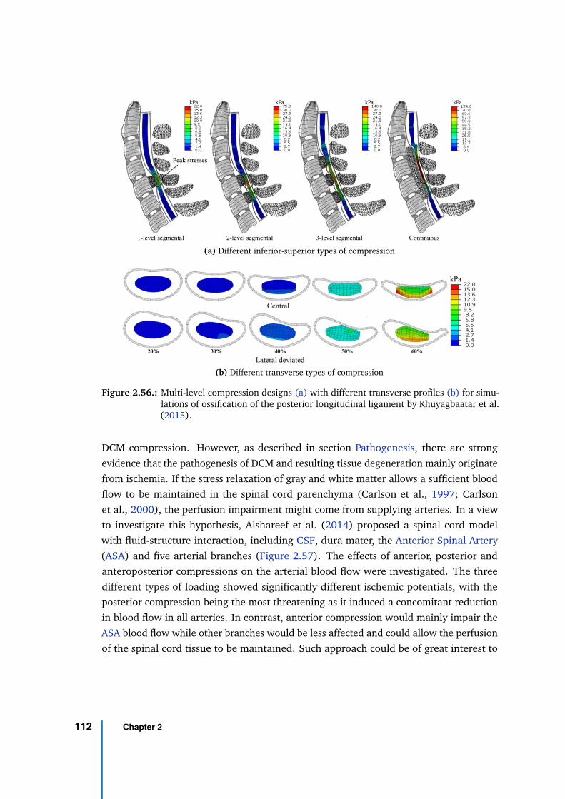
(a) Different inferior-superior types of compression

(b) Different transverse types of compression

Figure 2.56.: Multi-level compression designs (a) with different transverse profiles (b) for simu-lations of ossification of the posterior longitudinal ligament by Khuyagbaatar et al.(2015).

DCM compression. However, as described in section Pathogenesis, there are strong

evidence that the pathogenesis of DCM and resulting tissue degeneration mainly originate

from ischemia. If the stress relaxation of gray and white matter allows a sufficient blood

flow to be maintained in the spinal cord parenchyma (Carlson et al., 1997; Carlson

et al., 2000), the perfusion impairment might come from supplying arteries. In a view

to investigate this hypothesis, Alshareef et al. (2014) proposed a spinal cord model

with fluid-structure interaction, including CSF, dura mater, the Anterior Spinal Artery

(ASA) and five arterial branches (Figure 2.57). The effects of anterior, posterior and

anteroposterior compressions on the arterial blood flow were investigated. The three

different types of loading showed significantly different ischemic potentials, with the

posterior compression being the most threatening as it induced a concomitant reduction

in blood flow in all arteries. In contrast, anterior compression would mainly impair the

ASA blood flow while other branches would be less affected and could allow the perfusion

of the spinal cord tissue to be maintained. Such approach could be of great interest to

112 Chapter 2

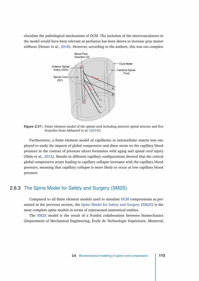
elucidate the pathological mechanisms of DCM. The inclusion of the microvasculature in

the model would have been relevant as perfusion has been shown to increase gray matter

stiffness (Hetzer et al., 2018). However, according to the authors, this was too complex.

Figure 2.57.: Finite element model of the spinal cord including anterior spinal arteries and fivebranches from Alshareef et al. (2014))

Furthermore, a finite element model of capillaries in extracellular matrix was em-

ployed to study the impacts of global compressive and shear strain on the capillary blood

pressure in the context of pressure ulcers formation with aging and spinal cord injury

(Shilo et al., 2012). Results in different capillary configurations showed that the critical

global compressive strain leading to capillary collapse increases with the capillary blood

pressure, meaning that capillary collapse is more likely to occur at low capillary blood

pressure.

2.6.3 The Spine Model for Safety and Surgery (SM2S)

Compared to all finite element models used to simulate DCM compressions as pre-

sented in the previous section, the Spine Model for Safety and Surgery (SM2S) is the

most complete spine models in terms of represented anatomical entities.

The SM2S model is the result of a fruitful collaboration between biomechanics

(Department of Mechanical Engineering, École de Technologie Supérieure, Montreal,


Quebec, Canada & Department of Mechanical Engineering, École Polytechnique, Mon-

treal, Quebec, Canada & Laboratoire de biomécanique appliquée, Aix-Marseille Université,

Marseille, France) and MRI (Centre de Résonance Magnétique en Biologie et Médecine,

Aix-Marseille Université, Marseille, France) research laboratories, as well as hospital

research centers (Department of Medical Engineering, Research Center, Hôpital du

Sacré-Cœur de Montréal, Montreal, Quebec, Canada & Research Center, Sainte-Justine

University Hospital Center, Montreal, Quebec, Canada), associated within an interna-

tional research laboratory (International Laboratory for Imaging and Biomechanics of the

Spine, iLab-Spine).

In constant development, the first version of the SM2S was published in 2009 (El-Rich

et al., 2009) (Figure 2.58a). Built out of the CT scan (with 0.6 mm-slice thicknesss) of

a 32-year old healthy male subject (Caucasian, 75.5 kg, 1.75 m), it included vertebrae,

intervertebral discs and ligaments of the lumbar spine segments L2 to L3. It was then

extended from T12 to L5 (Wagnac et al., 2012) (Figure 2.58b) and from T1 to L5

(Figure 2.58c) based on the same CT data (Wagnac, 2011). The spinal cord, with

distinction between white and gray matter based on histological cadaveric data (single

specimen) from literature (Kameyama et al., 1996), was then added along with pia mater,

dura mater, CSF, nerve roots and dentate ligaments (Fradet, 2013) (Figure 2.58d). The

model was then extended to the cervical region (Figure 2.58e) using the same methods

as for thoracic and lumbar regions (Sun, 2013). The anatomical CT data used were

acquired on a different subject but with similar characteristics and compatible geometrical

dimensions.

To refine the white and gray matter depiction — which was so far based on histological

data from a single subject, likely to be affected by tissue shrinkage due to harvesting — a

high-resolution T2*-weighted MRI template made out of transverse acquisitions at the

cervical level of 20 young healthy volunteers (Taso et al., 2015b) was used for white

and gray matter geometry at the cervical level (Taso, 2016) (Figure 2.58f). Finally, the

spinal cord was manually divided into 6 main functional regions based on the Gray’s

Anatomy atlas (Standring, 2008) and the unique spinal cord MRI atlas derived from it

(Lévy et al., 2015): anterior and posterior gray matter, and anterior, lateral and posterior

white matter (Taso, 2016; Rasoanandrianina, 2019) (Figure 2.58g).

Today, the SM2S is one of the most realistic model of the spine, with a detailed

anatomy from the sacrum to the highest cervical segment. It has been used in various

studies from crash simulation of traffic accident to ligament lesions.

114 Chapter 2

The SM2S (cervical segment from C4 to C6) has been first applied to DCM study by

Taso et al. (2015a). Intervertebral disc bulging, similar to the compressive mechanisms

occurring in DCM, was simulated by a global disc dislocation by 2 to 9 mm (with a velocity

of 0.05 mm/s) towards the cord which got compressed at various degrees. The degree of

compression was quantified by the ratio of antero-posterior cord diameter at compression

level over the initial diameter. The maximal compression obtained was 42% at C4-C5

and 61% at C5-C6. Results showed different von Mises and shear stresses distributions

between the two levels, due to morphological differences.

Interesting pioneering work was also conducted to combine multi-parametric MRI

maps acquired within Degenerative Cervical Myelopathy (DCM) patients to the biome-

chanical stresses obtained from spinal cord compression simulations (Taso et al., 2016).

Finally, important work has been carried out to refine the SM2S and apply it to different

traumatic spinal cord injuries (Beauséjour et al., 2020; Bailly et al., 2020).


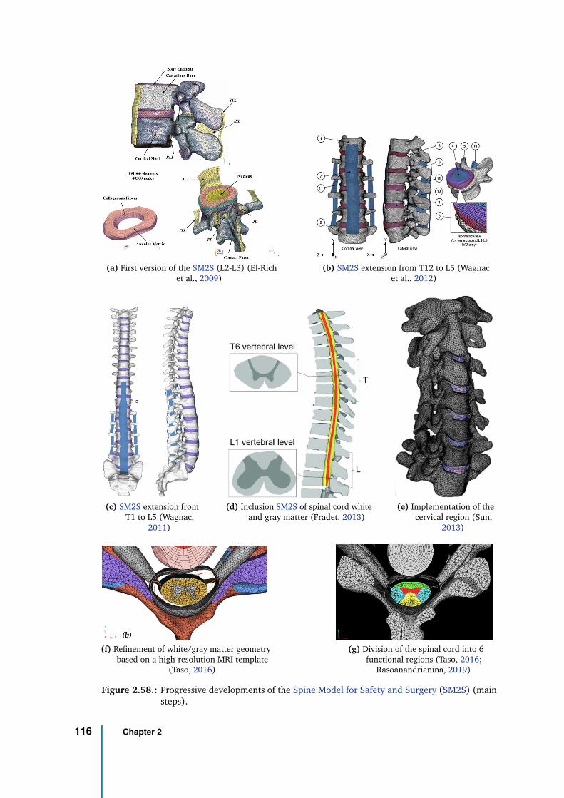
(a) First version of the SM2S (L2-L3) (El-Richet al., 2009)

(b) SM2S extension from T12 to L5 (Wagnacet al., 2012)

(c) SM2S extension fromT1 to L5 (Wagnac,

2011)

(d) Inclusion SM2S of spinal cord whiteand gray matter (Fradet, 2013)

(e) Implementation of thecervical region (Sun,

2013)

(f) Refinement of white/gray matter geometrybased on a high-resolution MRI template

(Taso, 2016)

(g) Division of the spinal cord into 6functional regions (Taso, 2016;

Rasoanandrianina, 2019)

Figure 2.58.: Progressive developments of the Spine Model for Safety and Surgery (SM2S) (mainsteps).

116 Chapter 2

Thesis objectives and structure 33.1 Research questions

In the context of chronic spinal cord compression such as occurring in Degenerative

Cervical Myelopathy (DCM), a widely accepted hypothesis is that the spine degenerations

apply mechanical constraints on spinal cord, which alter its perfusion, resulting in

microcirculation dysfunction or ischemic condition. In the long run, ischemia in turn

causes neuronal and oligodendroglial apoptosis on one hand, starting an inflammatory

reaction, and endothelial cell death on the other hand, leading to blood-spinal cord barrier

disruption. A vicious circle then starts, nourishing the inflammation which exacerbates the

cell death, eventually resulting in myelopathy. In mild compression cases, the perfusion

dysfunction might not be chronic but discontinuous in time at first, caused by repeated

micro-traumas with everyday life motion of the neck. In any case, the injury would

induce cell damage and trigger an inflammatory response.

Biomechanical simulations also strongly suggested mechanical stress applying within

the spinal cord parenchyma (Nishida et al., 2012; Kim et al., 2013; Khuyagbaatar et al.,

2015; Nishida et al., 2015a; Nishida et al., 2016), which might have injurious effect

on the tissue. Indeed, animal studies demonstrated a combined effect of ischemia and

mechanical constraints on tissue degeneration (Shimomura et al., 1968; Doppman, 1975).

Several key questions remain about the relation between the mechanical constraints

and hypoperfusion:

• Is the hypoperfusion mainly produced by the mechanical constraints applying within

the spinal cord tissue on the capillary network or by the compression of arterial

and/or venous vascular networks which alter the blood supply and drainage?

• Consequently, do the mechanical constraints within cord tissue have a direct effect

on tissue degeneration independent from the ischemic effect? Or is it strictly a

cause-effect relationship? Or a combination of both?

• What is the timeline of these events?

117

If these questions would require models to be fully controlled, explored, described and

understood, first questions oriented towards a better understanding and improvement of

diagnosis, treatment and prognosis of chronic spinal cord compression and which could

hopefully be answered through clinical investigations also arise:

• What is the extent of ischemia along the cord for a given compression value?

• What compression pattern is the most detrimental?

• Can new biomarkers be identified to help neurosurgeons in their decisions?

3.2 Objectives

To investigate the aforementioned questions, we thus propose to combine perfusion

Magnetic Resonance Imaging (MRI) with dedicated biomechanical models so as to

identify new key elements. However, based on the current research advances, the

following subsequent specific problems first need to be solved:

1) No technique (using MRI or other technology) capable of reliably map perfusion of

the human spinal cord exists.

2) The large interindividual variability in morphology and clinical presentation of

DCM patients requires realistic modeling of spinal cord compression to establish a

link between applied mechanical constraints and resulting tissue degeneration and

symptoms.

All together, while this thesis project presents with the global project objective to

inform the relation between mechanical constraints and ischemia in degenerative spinal

cord compression and its effects on tissue degeneration, in the perspective of identifying

risk factors, lesion criteria threshold and surgical guidelines, it more particularly aims two

specific objectives:

#1:

Implement a method to map perfusion in the human spinal cord.

#2:

Model typical DCM compressions using biomechanical finite element analysis.

118 Chapter 3

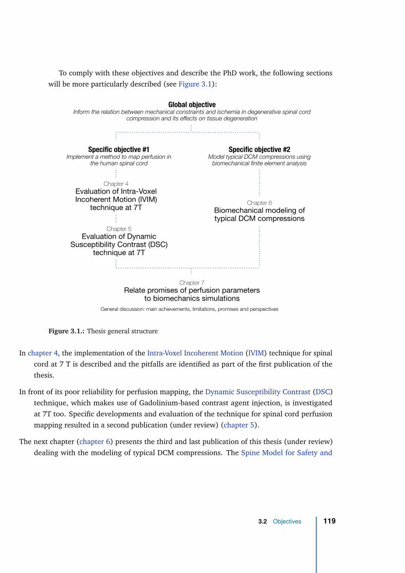
To comply with these objectives and describe the PhD work, the following sections

will be more particularly described (see Figure 3.1):

Global objective Inform the relation between mechanical constraints and ischemia in degenerative spinal cord

compression and its effects on tissue degeneration

Specific objective #1 Implement a method to map perfusion in

the human spinal cord

Specific objective #2 Model typical DCM compressions using

biomechanical finite element analysis

Chapter 4

Evaluation of Intra-Voxel Incoherent Motion (IVIM)

technique at 7T

Chapter 5

Evaluation of Dynamic Susceptibility Contrast (DSC)

technique at 7T

Chapter 6

Biomechanical modeling of typical DCM compressions

Chapter 7

Relate promises of perfusion parameters to biomechanics simulations

General discussion: main achievements, limitations, promises and perspectives

Figure 3.1.: Thesis general structure

In chapter 4, the implementation of the Intra-Voxel Incoherent Motion (IVIM) technique for spinal

cord at 7 T is described and the pitfalls are identified as part of the first publication of the

thesis.

In front of its poor reliability for perfusion mapping, the Dynamic Susceptibility Contrast (DSC)

technique, which makes use of Gadolinium-based contrast agent injection, is investigated

at 7T too. Specific developments and evaluation of the technique for spinal cord perfusion

mapping resulted in a second publication (under review) (chapter 5).

The next chapter (chapter 6) presents the third and last publication of this thesis (under review)

dealing with the modeling of typical DCM compressions. The Spine Model for Safety and

3.2 Objectives 119

Surgery (SM2S) is employed to simulate four compression patterns and a finite element

analysis is carried out to compare them and potentially identify the most detrimental processes.

Finally, the achievements of this thesis are discussed (chapter 7). Pitfalls and promises of IVIM

and DSC are raised. Potential of Arterial Spin Labeling (ASL) is described. The new insights

obtained from biomechanical simulations and stress analysis are outlined along with their

limitations. Last but not least, we will discuss the perspectives to reach the final stage of the

project where a decent comparison between applied mechanical constraints and impaired

perfusion could be possible.

120 Chapter 3

Intra-Voxel Incoherent Motion at

7 Tesla to quantify human

spinal cord perfusion:

limitations and promises

4

4.1 Foreword

This chapter introduces the first publication of the thesis, issued in the journal Magnetic

Resonance in Medicine on February 14, 2020.

Based on the recent achievements of diffusion MRI in the human spinal cord at 7T,

the Intra-Voxel Incoherent Motion (IVIM) technique appeared promising for perfusion

mapping. It was the first technique investigated in this thesis.

In this article, the IVIM technique was developed to be applied to the human spinal

cord in a whole-body MRI system. Monte-Carlo simulations were carried out to calibrate

the fitting of the IVIM model and estimate the error as a function of Signal-to-Noise Ratio

(SNR). After an empirical optimization of the acquisition protocol for SNR, in-vivo results

in six healthy volunteers were presented and compared to numerical simulations. Despite

a large SNR and number of b-values, the IVIM model was not reliable enough to provide

blood volume- and blood flow-related maps at a single-subject and single-slice averaging

level. Nevertheless, the average maps across six slices and six subjects increased the

reliability enough to reveal the higher perfusion of gray matter compared to white matter,

as expected according to results in mouse spinal cord and human brain.

This work was the subject of an oral presentation at the French Society for Magnetic

Resonance in Biology and Medicine (SFRMBM) Annual Meeting 2019 in Strasbourg,

France, at the International Society for Magnetic Resonance in Medicine (ISMRM) Ultra-

High Field Workshop 2019 in Dubrovnik, Croatia, at the ISMRM Annual Meeting 2019 in

Montreal, Canada and at the Spinal Cord MRI Workshop 2019 in Montreal, Canada.

4.2 Manuscript

121

Magn Reson Med. 2020;00:1–20. | 1wileyonlinelibrary.com/journal/mrm

Received: 16 August 2019 | Revised: 16 December 2019 | Accepted: 10 January 2020

DOI: 10.1002/mrm.28195

F U L L P A P E R

Intravoxel Incoherent Motion at 7 Tesla to quantify human spinal

cord perfusion: Limitations and promises

Simon Lévy1,2,3,4 | Stanislas Rapacchi1,2 | Aurélien Massire1,2,4 | Thomas Troalen5 | Thorsten Feiweier6 | Maxime Guye1,2 | Virginie Callot1,2,4

1Aix-Marseille Univ, CNRS, CRMBM, Marseille, France

2APHM, Hopital Universitaire Timone, CEMEREM, Marseille, France

3Aix-Marseille Univ, IFSTTAR, LBA, Marseille, France

4iLab-Spine International Associated Laboratory, Marseille-Montreal, France-Canada

5Siemens Healthcare SAS, Saint-Denis, France

6Siemens Healthcare GmbH, Erlangen, Germany

© 2020 International Society for Magnetic Resonance in Medicine

Correspondence

Virginie Callot, Centre de Résonance

Magnétique Biologique et Médicale

(CRMBM, UMR 7339, CNRS /

Aix-Marseille Université), 27 bd Jean

Moulin, 13385 Marseille cedex 05, France.

Email: [email protected]

Funding information

Investissements d’Avenir (A*MIDEX),

Grant/Award Number: n° ANR-11-

IDEX-0001-02; European Union’s Horizon

2020 research and innovation program,

Grant/Award Number: Marie Skłodowska-

Curie grant agreement Nº713750; Centre

National de la Recherche Scientifique;

France Life Imaging, Grant/Award Number:

7T-AMI-ANR-11-EQPX-0001, A*MIDEX-

EI-13-07-130115-08.38-7T-AMISTART

and ANR-11-INBS-0006; Conseil Régional

Provence-Alpes-Côte d’Azur; Horizon

2020, Grant/Award Number: 713750;

French National Research Agency; Centre

National de la Recherche Scientifique

Purpose: To develop a noninvasive technique to map human spinal cord (SC) perfusion

in vivo. More specifically, to implement an intravoxel incoherent motion (IVIM)

protocol at ultrahigh field for the human SC and assess parameters estimation errors.

Methods: Monte-Carlo simulations were conducted to assess estimation errors of

2 standard IVIM fitting approaches (two-step versus one-step fit) over the range of

IVIM values reported for the human brain and for typical SC diffusivities. Required

signal-to-noise ratio (SNR) was inferred for estimation of the parameters product,

fIVIMD* (microvascular fraction times pseudo-diffusion coefficient), within 10%

error margins. In-vivo IVIM imaging of the SC was performed at 7T in 6 volunteers.

An image processing pipeline is proposed to generate IVIM maps and register them

for an atlas-based region-wise analysis.

Results: Required b = 0 SNRs for 10% error estimation on fIVIMD* with the one-step

fit were 159 and 185 for diffusion-encoding perpendicular and parallel to the SC

axis, respectively. Average in vivo b = 0 SNR within cord was 141 ± 79, correspond-

ing to estimation errors of 12.7% and 14.7% according to numerical simulations.

Slice- and group-averaging reduced noise in IVIM maps, highlighting the difference

in perfusion between gray and white matter. Mean ± standard deviation fIVIM and

D* values across subjects within gray (respectively white) matter were 16.0 ± 1.7

(15.0 ± 1.6)% and 11.4 ± 2.9 (11.5 ± 2.4) × 10−3 mm2/s.

Conclusion: Single-subject data SNR at 7T was insufficient for reliable perfusion

estimation. However, atlas-averaged IVIM maps highlighted the higher microvascu-

lar fraction of gray matter compared to white matter, providing first results of healthy

human SC perfusion mapping with MRI.

K E Y W O R D S

7T MRI, intravoxel incoherent motion, IVIM, perfusion, spinal cord, ultrahigh field MRI

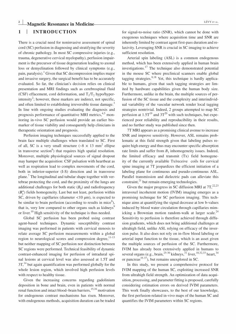
2 | LÉVY ET AL.

1 | INTRODUCTION

There is a crucial need for noninvasive assessment of spinal

cord (SC) perfusion in diagnosing and stratifying the severity

of chronic pathology. In most SC compressive injuries (e.g.,

trauma, degenerative cervical myelopathy), perfusion impair-

ment is the precursor of tissue degeneration leading to axonal

loss or demyelination followed by clinical symptoms (e.g.,

pain, paralysis).1 Given that SC decompression implies major

and invasive surgery, the surgical benefit has to be accurately

evaluated. So far, the clinician’s decision relies on clinical

presentation and MRI findings such as cerebrospinal fluid

(CSF) effacement, cord deformation, and T1/T2 hypo/hyper-

intensity2; however, these markers are indirect, not specific,

and often limited to establishing irreversible tissue damage.3

In line with ongoing studies evaluating the diagnosis and

prognosis performance of quantitative MRI metrics,4,5 mon-

itoring in-vivo SC perfusion would provide an earlier bio-

marker of tissue viability and consequently help clinicians in

therapeutic orientation and prognosis.

Perfusion imaging techniques successfully applied to the

brain face multiple challenges when translated to SC. First

of all, SC is a very small structure (~8 × 13 mm2 ellipse

in transverse section6) that requires high spatial resolution.

Moreover, multiple physiological sources of signal dropout

may hamper the acquisition: CSF pulsation with heartbeat as

well as respiration lead to complex movements of the cord,

both in inferior-superior (I-S) direction and in transverse

plane.7 The longitudinal and tubular shape together with ver-

tebrae protecting the cord, and the proximity of the lungs are

additional challenges for both static (B0) and radiofrequency

(B+

1) fields homogeneity. Last but not least, perfusion within

SC, driven by capillaries (diameter <10 µm), is expected to

be similar to brain perfusion (according to results in mice8),

that is, very low compared to other organs such as kidneys9

or liver.10 High sensitivity of the technique is thus needed.

Global SC perfusion has been probed using contrast

agent-based techniques. Dynamic susceptibility contrast

imaging was performed in patients with cervical stenosis to

relate average SC perfusion measurements within a global

region to neurological scores and compression degree,11-13

but neither mapping of SC perfusion nor distinction between

SC regions were performed. Technical feasibility of dynamic

contrast-enhanced imaging for perfusion of intradural spi-

nal lesions at cervical level was also assessed at 1.5T and

3T,14 but again quantification was performed globally for the

whole lesion region, which involved high perfusion levels

with respect to healthy tissue.

Given the increasing concerns regarding gadolinium

deposition in bone and brain, even in patients with normal

renal function and intact blood–brain barriers,15,16 motivation

for endogenous contrast mechanisms has risen. Moreover,

with endogenous methods, acquisition duration can be traded

for signal-to-noise ratio (SNR), which cannot be done with

exogenous techniques where acquisition time and SNR are

inherently limited by contrast agent first-pass duration and re-

laxivity. Leveraging SNR is crucial in SC imaging to achieve

sufficient resolution.

Arterial spin labeling (ASL) is a common endogenous

method, which has been extensively applied in human brain

investigations.17 The technique also demonstrated potential

in the mouse SC where preclinical scanners enable global

tagging strategies.8,18 Yet, this technique is hardly applica-

ble to humans, given that such tagging strategies are lim-

ited by hardware capabilities given the human body size.

Furthermore, unlike in the brain, the multiple sources of per-

fusion of the SC tissue and the complexity and interindivid-

ual variability of the vascular network render local tagging

strategies nontrivial. Indeed, 2 groups attempted to map SC

perfusion at 1.5T19 and 3T20 with such techniques, but expe-

rienced poor reliability and reproducibility in their results,

and no further study was published since then.

7T MRI appears as a promising clinical avenue to increase

SNR and improve sensitivity. However, ASL remains prob-

lematic at this field strength given that labeling pulses re-

quire high energy and thus may encounter specific absorption

rate limits and suffer from B1 inhomogeneity issues. Indeed,

the limited efficacy and transmit (Tx) field homogene-

ity of the currently available Tx/receive coils for cervical

spine imaging at 7T jeopardizes the efficient initiation of a

labeling plane for continuous and pseudo-continuous ASL.

Parallel transmission and dielectric pads can alleviate this

constraint,21 but remain emerging technologies.

Given the major progress in SC diffusion MRI at 7T,22,23

intravoxel incoherent motion (IVIM) imaging emerges as a

promising technique for SC perfusion imaging. This tech-

nique aims at quantifying the signal decrease at low b-values

induced by blood water circulation through capillaries mim-

icking a Brownian motion random-walk at larger scale.24

Sensitivity to perfusion is therefore achieved through diffu-

sion gradients, which does not bring additional challenges at

ultrahigh field, unlike ASL relying on efficacy of the inver-

sion pulse. It also does not rely on in-flow blood labeling or

arterial input function to the tissue, which is an asset given

the multiple sources of perfusion of the SC. Furthermore,

IVIM has already been extensively applied in humans to

several organs (e.g., brain,25-30 kidneys,31 liver,10,32,33 heart,34

or pancreas35-37), but remains unexplored in SC.

In this study, we present a comprehensive protocol for

IVIM mapping of the human SC, exploiting increased SNR

from ultrahigh field strength. An optimization of data acqui-

sition, processing, and parameter fitting is proposed, carefully

considering estimation errors on derived IVIM parameters.

This work finally showcases, to the best of our knowledge,

the first perfusion-related in-vivo maps of the human SC and

quantifies the IVIM parameters within SC regions.

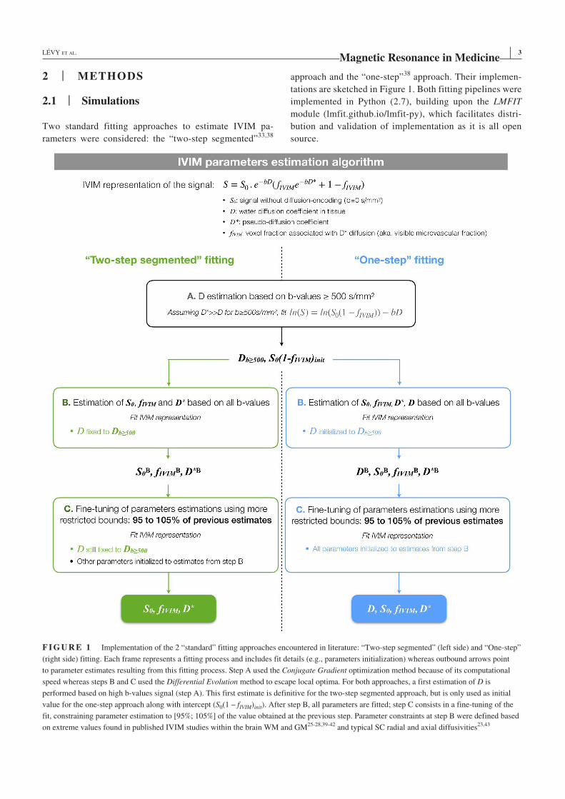
| 3LÉVY ET AL.

2 | METHODS

2.1 | Simulations

Two standard fitting approaches to estimate IVIM pa-

rameters were considered: the “two-step segmented”33,38

approach and the “one-step”38 approach. Their implemen-

tations are sketched in Figure 1. Both fitting pipelines were

implemented in Python (2.7), building upon the LMFIT

module (lmfit.github.io/lmfit-py), which facilitates distri-

bution and validation of implementation as it is all open

source.

F I G U R E 1 Implementation of the 2 “standard” fitting approaches encountered in literature: “Two-step segmented” (left side) and “One-step”

(right side) fitting. Each frame represents a fitting process and includes fit details (e.g., parameters initialization) whereas outbound arrows point

to parameter estimates resulting from this fitting process. Step A used the Conjugate Gradient optimization method because of its computational

speed whereas steps B and C used the Differential Evolution method to escape local optima. For both approaches, a first estimation of D is

performed based on high b-values signal (step A). This first estimate is definitive for the two-step segmented approach, but is only used as initial

value for the one-step approach along with intercept (S0(1 – fIVIM)init). After step B, all parameters are fitted; step C consists in a fine-tuning of the

fit, constraining parameter estimation to [95%; 105%] of the value obtained at the previous step. Parameter constraints at step B were defined based

on extreme values found in published IVIM studies within the brain WM and GM25-28,39-42 and typical SC radial and axial diffusivities23,43

4 | LÉVY ET AL.

Software and implementations can have a significant

impact on accuracy and precision of parameter estima-

tions25,28,39 regardless of computational speed. Therefore,

inspired by the work of Pekar et al,38 we performed Monte-

Carlo simulations to assess their performance under different

physiological and SNR conditions. Ranges of possible values

for IVIM parameters were defined according to ranges of val-

ues found in brain literature25-28,39-42 and typical SC radial

and axial diffusivities23,43:

• Visible microvascular volume fraction fIVIM (%): 1 to 30.

• Pseudo-diffusion coefficient D* (mm2/s): 3.0 × 10−3 to

35.0 × 10−3.

• Pure diffusion coefficient D (mm2/s): 0.3 × 10−3

(D⊥, diffusivity in the SC transverse plane) and 1.5 × 10−3

(D||, diffusivity along the SC axis).

The IVIM representation of the signal24 is given by

(Equation 1):

To assess performance of fitting algorithm, synthetic data were

generated using (Equation 1) and ranging a large number of

b-values inspired by IVIM protocols in brain25,26,40,44 and dif-

fusion tensor imaging (DTI) practice in SC45,46: 5, 10, 15, 20,

30, 50, 75, 100, 125, 150, 200, 250, 600, 700, and 800 s/mm2.

Given that the in-vivo fitted data result from the averaging of

multiple repetitions of magnitude images, according to the

central limit theorem, the noise distribution in such data can

be assumed Gaussian. Therefore, random Gaussian noise was

added to synthetic data with standard deviation (SD) matching

realistic SNR as described below. Finally, mean absolute esti-

mation error across N = 1000 random noise draws was calcu-

lated for each fitted parameter according to (Equation 2):

Three types of simulations were performed:

1. Estimation errors were assessed with infinite SNR

(SDnoise = 0) for both fitting approaches and for all pa-

rameter values within the defined ranges. These simula-

tions served to verify whether algorithms could retrieve

true parameter values on perfect data given the b-value

distribution used.

2. Estimations errors were assessed for realistic SNR values

of 60, 120, and 180. These values corresponded to the min-

imum, mean, and maximum across subjects of the average

voxel-wise SNR within SC measured in vivo at b ≈ 0.

3. The minimum required SNR for b = 0 data to get an error

≤ 10% on the parameter fIVIMD* (product of fIVIM and D*,

related to blood flow47) was computed for all parameter

values within the defined ranges and for the one-step

approach.

To get the corresponding required SNR for higher

b-values (e.g., b = 800 s/mm2 with D = 1.5 × 10−3 mm2/s in

the SC for diffusion weighting along I-S direction), one just

needs to multiply it by e−bD (i.e., here 0.3), assuming that

the microvascular compartment contribution to the signal

at such high b-values can be neglected (D* >> D). SNR of

diffusion-weighted images depends on the orientation of

the diffusion gradient (as accounted for in the diffusion

coefficient D).

Fitting algorithms (Figure 1) were optimized through

simulations 1 and 2, especially regarding the fit optimi-

zation method (e.g., trust-region reflective least squares,

Levenberg–Marquardt, Brute Force). The differential evolu-

tion method,48 as implemented in the LMFIT module, was

preferred to avoid local optima solutions and to provide speed

and precision in parameters estimation.

2.2 | Data acquisition

2.2.1 | Population and MR setup

The study was approved by the local ethics committee, and

written consents were obtained from 8 healthy volunteers be-

fore MR examinations. Two subjects (1 male, 1 female) were

dedicated to optimization of acquisition parameters, and

6 (5 males, 1 female, mean age ± SD = 25.0 ± 2.6 years old)

were scanned with the optimized protocol. Acquisitions were

performed on a 7T whole-body research system (Siemens

Healthcare, Erlangen, Germany) with a commercial 8-channel

cervical-spine transceiver surface coil (Rapid Biomedical

GmbH, Rimpar, Germany) used with the 8 Tx-channels hard-

ware combined into a single Tx system. The complete pro-

tocol (see more details in Supporting Information Table S1)

included:

- Patient-specific tuning: localizer for slice positioning,

coil voltage calibration, local B0 shimming within a

~4 × 3 × 5 cm3 (Right-Left × Anterior-Posterior × I-S)

volume around the cord, B+

1 and B0 maps to inspect

fields inhomogeneities and shimming performance.

- Sagittal 2D turbo-spin echo imaging with 0.6 × 0.6 mm2

in-plane resolution and 2.2-mm slice thickness for verte-

bral levels localization.

- Pulse-triggered IVIM protocol (further described below).

(1)S=Sb=0e−b⋅D(

fIVIMe−b⋅D∗

+1− fIVIM

)

(2)error (%)=100

N×

N∑

i=1

||estimated valuei− true value||

true value

| 5LÉVY ET AL.

- Axial 2D high-resolution (0.4 × 0.4 mm2 in-plane, 5-mm

slice thickness) multiecho gradient-echo (MGE) image for

gray matter (GM) segmentation.

Depending on the subject’s heartbeat, total protocol time was

1 hour and 10 to 15 minutes.

2.2.2 | IVIM acquisition protocol

IVIM acquisitions were based on a prototype 2D single-shot

diffusion-prepared spin-echo echo planar imaging (EPI) se-

quence. Six slices (5-mm thick with 1-mm gap) were cen-

tered at C3-C4 intervertebral disk (area minimizing partial

volume effects induced by cord curvature in this cohort).

C3 to C4 coverage was guaranteed for all subjects. Phase

was encoded along the right-left (R-L) axis for robust paral-

lel imaging given the coil configuration (see coil diagram in

Massire et al22).

Given that a low spinal cord perfusion level is expected

according to brain studies,25,49,50 sequence parameters were

experimentally optimized to maximize SNR (Supporting

Information Figure S1A). The following acquisition param-

eters were investigated: diffusion scheme, minimal band-

width, generalized autocalibrating partial parallel acquisition

(GRAPPA) factor, partial Fourier, outer volume suppression

with reduced field of view (FOV) strategy, number of lines

for GRAPPA calibration scans, and partial Fourier recon-

struction algorithm. Regarding diffusion scheme, given that

SNR decreases with longer TE, only short TE schemes were

considered: the standard Stejskal–Tanner scheme (monopo-

lar) and a modified version of it (“monopolar+”), applying

diffusion gradients during the entire time between excitation

and refocusing pulses, leaving no dead time.51 With the op-

timized parameter set, a minimum TE of 51.6 ms (effective

δ/Δ = 12.2/13.3 ms) and an SNR gain of 27% compared to the

“base” protocol were obtained (see Supporting Information

Figure S1A; Supporting Information Table S1).

To mitigate effects of SC motion and CSF pulsation,

acquisitions were synchronized on cardiac beat monitored

with a pulse oximeter (no trigger delay). The number of

cycles to acquire all slices NRR (determining the effective

TR for each slice) was adapted to each subject’s heartbeat

duration TRR so as to get the highest SNR efficiency (SNR/

time unit), which was calculated using the spin-echo sig-

nal expression derived from Bloch equations for a single

refocusing pulse52 and SC T1 values from the literature22

(Supporting Information Figure S1B). The resulting effec-

tive TR per slice was 2.6 seconds on average. Considering

that the maximum variation of TRR in healthy subjects would

be approximately 0.2 seconds, with a T1 in the SC around

1.25 seconds,22 the variations in longitudinal relaxation

would be, in the worst-case scenario (effective TR variation

of 0.6s with NRR = 3), around 6% at maximum (1−e−TReff ∕T1 ).

Moreover, these potential variations would be eventually

mitigated by the averaging over multiple repetitions in final

data. Consequently, signal relaxation variations attributable

to effective TR variations along acquisition were considered

negligible in this study.

Finally, b-value distribution was empirically defined,

inspired by IVIM protocols in brain25,26,40,44 and DTI prac-

tice in SC,45,53 so as to focus sampling on low b-values

(≤250 s/mm2) to better probe the fast decaying signal related

to perfusion. The number of b-values, Nb, was also empir-

ically defined in direct relation with the number of repeti-

tions Nrep per b-value, limiting the scan time to a maximum

of 1 hour for the IVIM protocol, which included 3 orthogonal

diffusion-encoding directions (R-L, anterior-posterior [A-P],

and I-S), that is: Nb ⋅Nrep ⋅NRR ⋅TRR ⋅3<1 hour.

B-values were corrected to include imaging gradient con-

tributions. Eventually, actual b-value distribution was 5, 10,

15, 20, 30, 50, 75, 100, 125, 150, 200, 250, 600, 700, and

800 s/mm2 with 30 repetitions per b-value, allowing slight

variations between subjects and directions as explained

above. Furthermore, to correct for EPI readout-related dis-

tortions, acquisitions were split into 2 distinct imaging sets

of equal lengths (Nrep/2), in forward (right>left) and reverse

(left>right) phase-encoding direction for each diffusion-

encoding direction.

2.3 | Data postprocessing

First, diffusion-weighted data were denoised using the

local principal component analysis algorithm developed by

Manjón et al54 across repetitions, for each b-value and in-

dependently for each phase-encoding direction. Second, the

subpixel shifting method from Kellner et al55 was applied to

remove any potential Gibbs-ringing artifact. Third, a dedi-

cated program (sct_dmri_moco) available within the Spinal

Cord Toolbox56 (v3.1.1) was used for correction of cord mo-

tion throughout the acquisition. Fourth, EPI readout-related

distortions were corrected using the topup program from

FSL57 based on forward and reverse phase-encoded b = 0 im-

ages and applying the least-square restoration method. Fifth

and final step, all repetitions of equal b-value were averaged,

ending up with 1 volume (6 slices) per b-value and diffusion-

encoding direction.

2.4 | In-vivo SNR and data fitting

As defined by Reeder et al,58 in-vivo SNR was calculated

voxelwise as the ratio of the mean signal across repetitions

6 | LÉVY ET AL.

to the SD across repetitions. Calculation was performed on

the lowest b-value images obtained, after the postprocess-

ing pipeline was applied. A factor of √

Nrep was applied to

reflect the SNR value of the average across all repetitions,

which is used as input data to the fitting algorithm. Voxel-

wise SNR was averaged per subject across the entire SC,

and the minimum, maximum, and mean values across sub-

jects served as references for the simulations (Section 2.1).

Based on simulation results (Section 3.1), in-vivo data

were fitted voxelwise using the one-step approach described

in Figure 1. Five IVIM parameter 3D maps (fIVIM, D*, D, S0

and fIVIMD*) were produced for each subject and each diffu-

sion-encoding direction.

2.5 | Quantification

For group analysis and quantification within regions of in-

terest (ROIs), IVIM maps were registered to the PAM50

template59 and its white matter (WM) atlas60 using dedicated

tools from the Spinal Cord Toolbox56,61,62 (v3.1.1) as de-

scribed in Figure 2.

3 | RESULTS

3.1 | The one-step fitting approach performs better for the range of IVIM values expected in the human SC

For IVIM parameter values expected in the human SC,

the one-step fitting approach showed better estimation

performance than the two-step segmented approach, both

on perfect (SNR = ∞) and noisy data (SNR levels meas-

ured in vivo). This comparison can be found in Supporting

Information Figure S2. The higher performance of the one-

step approach is observed on all parameters, especially

on D, which is attributable to the low sampling of high

b-values (only 3 b-values ≥600 s/mm2); the inaccuracy in

D then propagates more importantly on the other param-

eters with the two-step segmented approach. Consequently,

given the b-value distribution used, the one-step fitting ap-

proach is more appropriate for IVIM parameters fitting in

the human SC.

More in details for the one-step fitting approach (Figure 3),

the algorithm perfectly retrieves the true values of parameters

with infinite SNR and estimation errors increase when SNR

decreases. The parameter estimated with highest precision is

D, then fIVIM and then fIVIMD*, and the parameter estimated

with the largest error is D*, as commonly reported in the IVIM

literature. Interestingly, for high D values (D||), the error on

D is lower than for low D values (D⊥) whereas it is higher for

fIVIM, D* and fIVIMD*. Indeed, signal decay induced by high

D is sharper at high b-values, but then the effect of the other

IVIM parameters on the signal is more challenging to extract.

Furthermore, errors increase when perfusion levels (fIVIM,

D*, fIVIMD*) decrease, given that signal decay gets slower

and smaller. For instance, with high SNR (180) and low D

(0.3 × 10−3 mm2/s), estimation errors on fIVIM, D*, and fIVIMD*

exceed 100% (squares above orange levels) when (fIVIM, D*) is

lower than (4.2%, 6.6 × 10−3 mm2/s), (13.9%, 13.7 × 10−3 mm2/s),

and (1%, 6.6 × 10−3 mm2/s), respectively. Finally,

when fIVIM is around 16% and D* around 11.5 × 10−3 mm2/s

(as measured in vivo, see below) and potentially lower

(~10%), the expected error on fIVIM, D*, and fIVIMD* is around

15%, 30%, and 10% with SNR = 180, respectively.

3.2 | High SNR is required for accurate estimation of fIVIMD*

In the range of considered IVIM values, high b = 0 SNR

(≥70) is required to estimate fIVIMD* within 10% error

margins (Figure 4). SNR higher than 400 is needed if

fIVIM ≤ 7.4% and/or D* ≤ 3.0 × 10−3 mm2/s.

Because of crosstalk between fIVIM and D* (shared sen-

sitivity to the same physiological process), their individual

error can exceed 10% whereas their product fIVIMD* offers

an accuracy below 10% (e.g., for fIVIM, D* = 13.9%, 10.1 ×

10−3 mm2/s).

Of note, increased D requires higher SNR for the same

accuracy, which stands as a challenge for IVIM along the SC

axis. Figure 4 also shows that fIVIM is preponderant over D* in

determining the required SNR.

3.3 | In-vivo SNR

Figure 5 shows an example of single-subject and single-

slice b = 0 images along with the corresponding SNR,

signal, and noise maps at the different steps of the post-

processing pipeline. Mean SNR in SC for this particular

subject and slice was 10 ± 3 at acquisition, 30 ± 13 after

denoising and removal of Gibbs artefacts, and 147 ± 68

after distortion correction and averaging across repetitions.

At the group level, the minimum, mean, and maximum

SNR across subjects and IVIM acquisitions (diffusion-

encoding directions) on the lowest b-value images at out-

put of the postprocessing pipeline were approximately 60,

120, and 180 (see the SNR distribution of the entire cohort

in Supporting Information Figure S3). Estimation errors

on IVIM parameters for such SNR values are given by

Figure 3.

Group-averaged maps (Figure 6A) show that high SNR

values were obtained fairly homogeneously inside the cord,

generally at 1 to 2 voxel distance from the edge (in native

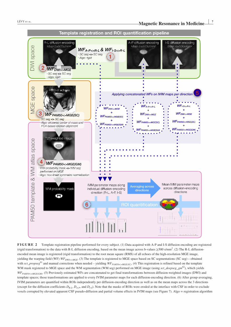
| 7LÉVY ET AL.

F I G U R E 2 Template registration pipeline performed for every subject. (1) Data acquired with A-P and I-S diffusion encoding are registered

(rigid transformation) to the data with R-L diffusion encoding, based on the mean image across b-values ≥500 s/mm2. (2) The R-L diffusion-

encoded mean image is registered (rigid transformation) to the root mean square (RMS) of all echoes of the high-resolution MGE image,

yielding the warping field (WF) WFDWI<>MGE. (3) The template is registered to MGE space based on SC segmentations (SC seg) – obtained

with sct_propseg61 and manual corrections when needed – yielding WFPAM50<>MGE(SC). (4) This registration is refined based on the template

WM mask registered to MGE space and the WM segmentation (WM seg) performed on MGE image (using sct_deepseg_gm62), which yields

WFPAM50<>MGE(GM). (5) Previously estimated WFs are concatenated to get final transformations between diffusion-weighted images (DWI) and

template spaces; those transformations are applied to every IVIM parameter maps for each diffusion-encoding direction. (6) After group-averaging,

IVIM parameters are quantified within ROIs independently per diffusion-encoding direction as well as on the mean maps across the 3 directions

(except for the diffusion coefficients DR-L, DA-P, and DI-S). Note that the masks of ROIs were eroded at the interface with CSF in order to exclude

voxels corrupted by elevated apparent CSF pseudo-diffusion and partial volume effects in IVIM maps (see Figure 7). Algo = registration algorithm

8 | LÉVY ET AL.

FI

GU

RE

3

Est

imat

ion e

rrors

on e

ach I

VIM

par

amet

er a

ccord

ing t

o (

f IV

IM, D

*, D

) tr

ue

val

ues

for

the

one-

step

fit

ting a

ppro

ach w

ith d

iffe

rent

SN

R l

evel

s: ∞

(no n

ois

e), 180 (

max

imum

in v

ivo

SN

R),

120 (

mea

n),

and 6

0 (

min

imum

). O

n t

he

y-ax

is o

f ea

ch g

raph, f I

VIM

var

ies

from

1%

to 3

0%

wher

eas

on t

he

x-ax

is D

* v

arie

s fr

om

3 t

o 3

5 ×

10

−3 m

m2/s

(bounds

def

ined

acc

ord

ing t

o I

VIM

lite

ratu

re i

n b

rain

WM

and G

M a

s des

crib

ed i

n S

ecti

on 2

.1);

on t

he

left

sid

e, D

= 0

.3 ×

10

−3 m

m2/s

, si

mil

ar t

o d

iffu

sivit

y i

n S

C t

ransv

erse

pla

ne

(D⊥),

wher

eas

on t

he

right

side

D =

1.5

× 1

0−

3 m

m2/s

,

sim

ilar

to d

iffu

sivit

y a

long S

C a

xis

(D

||).

Med

ian [

min

-max

] er

rors

are

indic

ated

on t

op o

f ea

ch g

raph

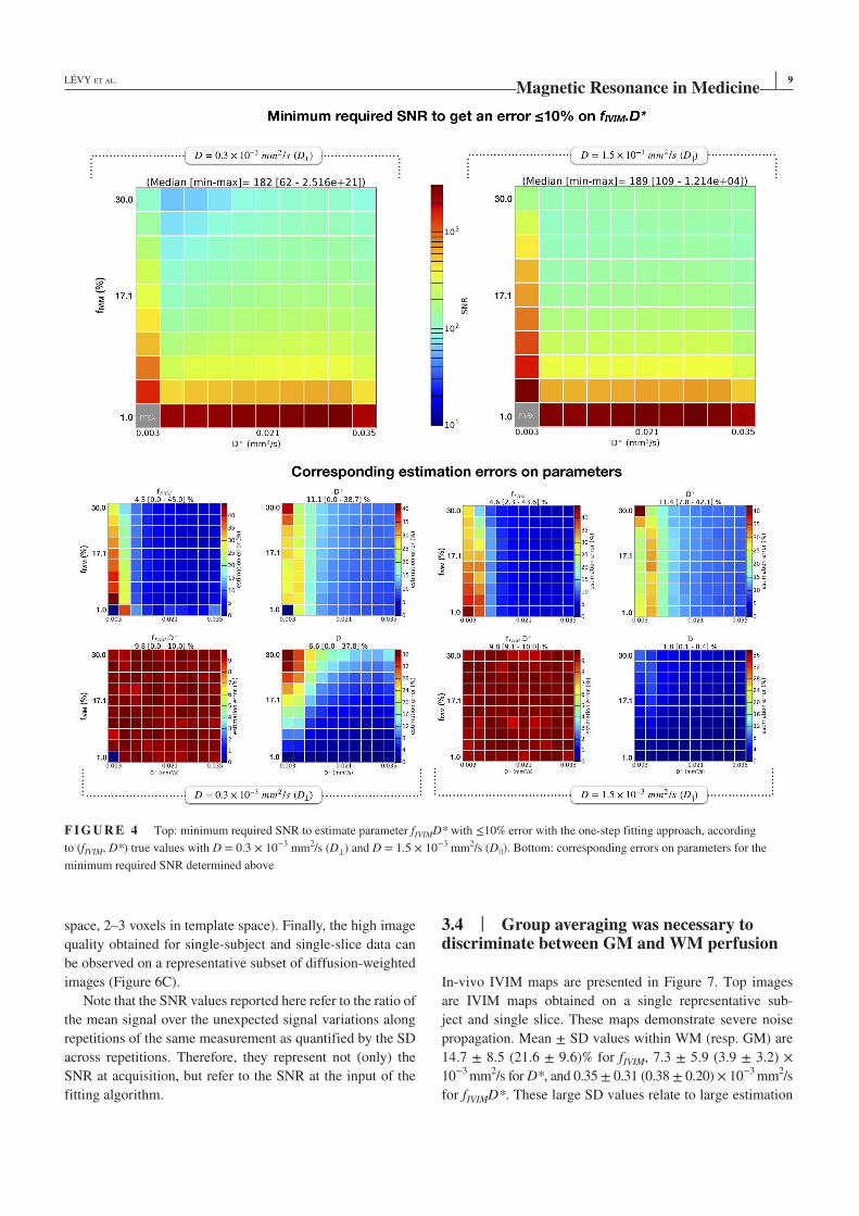
| 9LÉVY ET AL.

space, 2–3 voxels in template space). Finally, the high image

quality obtained for single-subject and single-slice data can

be observed on a representative subset of diffusion-weighted

images (Figure 6C).

Note that the SNR values reported here refer to the ratio of

the mean signal over the unexpected signal variations along

repetitions of the same measurement as quantified by the SD

across repetitions. Therefore, they represent not (only) the

SNR at acquisition, but refer to the SNR at the input of the

fitting algorithm.

3.4 | Group averaging was necessary to discriminate between GM and WM perfusion

In-vivo IVIM maps are presented in Figure 7. Top images

are IVIM maps obtained on a single representative sub-

ject and single slice. These maps demonstrate severe noise

propagation. Mean ± SD values within WM (resp. GM) are

14.7 ± 8.5 (21.6 ± 9.6)% for fIVIM, 7.3 ± 5.9 (3.9 ± 3.2) ×

10−3 mm2/s for D*, and 0.35 ± 0.31 (0.38 ± 0.20) × 10−3 mm2/s

for fIVIMD*. These large SD values relate to large estimation

F I G U R E 4 Top: minimum required SNR to estimate parameter fIVIMD* with ≤10% error with the one-step fitting approach, according

to (fIVIM, D*) true values with D = 0.3 × 10−3 mm2/s (D⊥) and D = 1.5 × 10−3 mm2/s (D||). Bottom: corresponding errors on parameters for the

minimum required SNR determined above

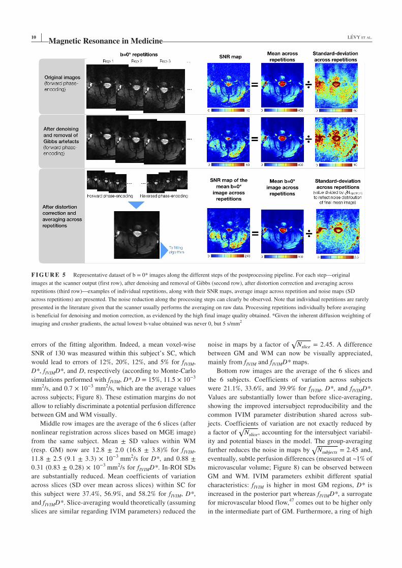
10 | LÉVY ET AL.

errors of the fitting algorithm. Indeed, a mean voxel-wise

SNR of 130 was measured within this subject’s SC, which

would lead to errors of 12%, 20%, 12%, and 5% for fIVIM,

D*, fIVIMD*, and D, respectively (according to Monte-Carlo

simulations performed with fIVIM, D*, D = 15%, 11.5 × 10−3

mm2/s, and 0.7 × 10−3 mm2/s, which are the average values

across subjects; Figure 8). These estimation margins do not

allow to reliably discriminate a potential perfusion difference

between GM and WM visually.

Middle row images are the average of the 6 slices (after

nonlinear registration across slices based on MGE image)

from the same subject. Mean ± SD values within WM

(resp. GM) now are 12.8 ± 2.0 (16.8 ± 3.8)% for fIVIM,

11.8 ± 2.5 (9.1 ± 3.3) × 10−3 mm2/s for D*, and 0.88 ±

0.31 (0.83 ± 0.28) × 10−3 mm2/s for fIVIMD*. In-ROI SDs

are substantially reduced. Mean coefficients of variation

across slices (SD over mean across slices) within SC for

this subject were 37.4%, 56.9%, and 58.2% for fIVIM, D*,

and fIVIMD*. Slice-averaging would theoretically (assuming

slices are similar regarding IVIM parameters) reduced the

noise in maps by a factor of √

Nslice

= 2.45. A difference

between GM and WM can now be visually appreciated,

mainly from fIVIM and fIVIMD* maps.

Bottom row images are the average of the 6 slices and

the 6 subjects. Coefficients of variation across subjects

were 21.1%, 33.6%, and 39.9% for fIVIM, D*, and fIVIMD*.

Values are substantially lower than before slice-averaging,

showing the improved intersubject reproducibility and the

common IVIM parameter distribution shared across sub-

jects. Coefficients of variation are not exactly reduced by

a factor of √

Nslice

, accounting for the intersubject variabil-

ity and potential biases in the model. The group-averaging

further reduces the noise in maps by √

Nsubjects = 2.45 and,

eventually, subtle perfusion differences (measured at ~1% of

microvascular volume; Figure 8) can be observed between

GM and WM. IVIM parameters exhibit different spatial

characteristics: fIVIM is higher in most GM regions, D* is

increased in the posterior part whereas fIVIMD*, a surrogate

for microvascular blood flow,47 comes out to be higher only

in the intermediate part of GM. Furthermore, a ring of high

F I G U R E 5 Representative dataset of b = 0* images along the different steps of the postprocessing pipeline. For each step—original

images at the scanner output (first row), after denoising and removal of Gibbs (second row), after distortion correction and averaging across

repetitions (third row)—examples of individual repetitions, along with their SNR maps, average image across repetition and noise maps (SD

across repetitions) are presented. The noise reduction along the processing steps can clearly be observed. Note that individual repetitions are rarely

presented in the literature given that the scanner usually performs the averaging on raw data. Processing repetitions individually before averaging

is beneficial for denoising and motion correction, as evidenced by the high final image quality obtained. *Given the inherent diffusion weighting of

imaging and crusher gradients, the actual lowest b-value obtained was never 0, but 5 s/mm2

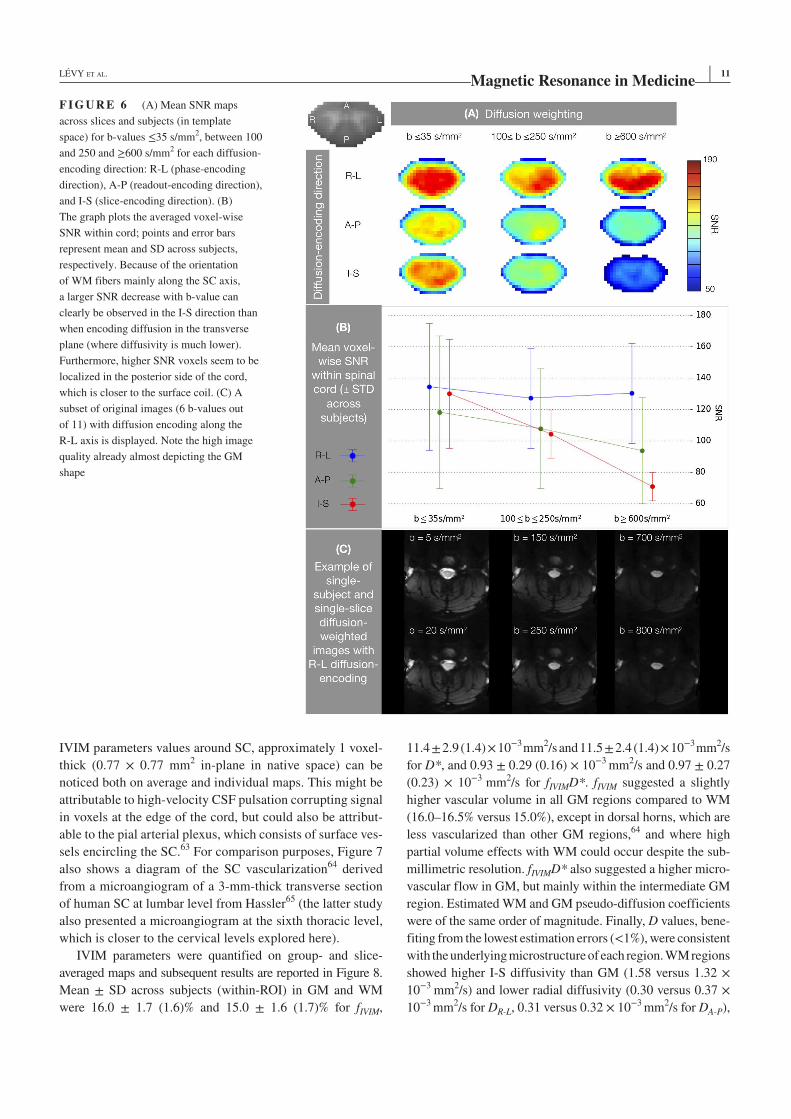
| 11LÉVY ET AL.

IVIM parameters values around SC, approximately 1 voxel-

thick (0.77 × 0.77 mm2 in-plane in native space) can be

noticed both on average and individual maps. This might be

attributable to high-velocity CSF pulsation corrupting signal

in voxels at the edge of the cord, but could also be attribut-

able to the pial arterial plexus, which consists of surface ves-

sels encircling the SC.63 For comparison purposes, Figure 7

also shows a diagram of the SC vascularization64 derived

from a microangiogram of a 3-mm-thick transverse section

of human SC at lumbar level from Hassler65 (the latter study

also presented a microangiogram at the sixth thoracic level,

which is closer to the cervical levels explored here).

IVIM parameters were quantified on group- and slice-

averaged maps and subsequent results are reported in Figure 8.

Mean ± SD across subjects (within-ROI) in GM and WM

were 16.0 ± 1.7 (1.6)% and 15.0 ± 1.6 (1.7)% for fIVIM,

11.4 ± 2.9 (1.4) × 10−3 mm2/s and 11.5 ± 2.4 (1.4) × 10−3 mm2/s

for D*, and 0.93 ± 0.29 (0.16) × 10−3 mm2/s and 0.97 ± 0.27

(0.23) × 10−3 mm2/s for fIVIMD*. fIVIM suggested a slightly

higher vascular volume in all GM regions compared to WM

(16.0–16.5% versus 15.0%), except in dorsal horns, which are

less vascularized than other GM regions,64 and where high

partial volume effects with WM could occur despite the sub-

millimetric resolution. fIVIMD* also suggested a higher micro-

vascular flow in GM, but mainly within the intermediate GM

region. Estimated WM and GM pseudo-diffusion coefficients

were of the same order of magnitude. Finally, D values, bene-

fiting from the lowest estimation errors (<1%), were consistent

with the underlying microstructure of each region. WM regions

showed higher I-S diffusivity than GM (1.58 versus 1.32 ×

10−3 mm2/s) and lower radial diffusivity (0.30 versus 0.37 ×

10−3 mm2/s for DR-L, 0.31 versus 0.32 × 10−3 mm2/s for DA-P),

F I G U R E 6 (A) Mean SNR maps

across slices and subjects (in template

space) for b-values ≤35 s/mm2, between 100

and 250 and ≥600 s/mm2 for each diffusion-

encoding direction: R-L (phase-encoding

direction), A-P (readout-encoding direction),

and I-S (slice-encoding direction). (B)

The graph plots the averaged voxel-wise

SNR within cord; points and error bars

represent mean and SD across subjects,

respectively. Because of the orientation

of WM fibers mainly along the SC axis,

a larger SNR decrease with b-value can

clearly be observed in the I-S direction than

when encoding diffusion in the transverse

plane (where diffusivity is much lower).

Furthermore, higher SNR voxels seem to be

localized in the posterior side of the cord,

which is closer to the surface coil. (C) A

subset of original images (6 b-values out

of 11) with diffusion encoding along the

R-L axis is displayed. Note the high image

quality already almost depicting the GM

shape

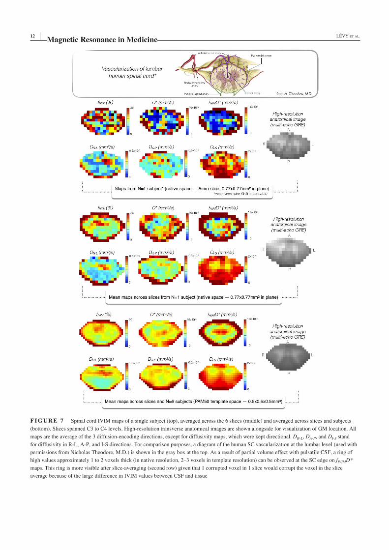
12 | LÉVY ET AL.

F I G U R E 7 Spinal cord IVIM maps of a single subject (top), averaged across the 6 slices (middle) and averaged across slices and subjects

(bottom). Slices spanned C3 to C4 levels. High-resolution transverse anatomical images are shown alongside for visualization of GM location. All

maps are the average of the 3 diffusion-encoding directions, except for diffusivity maps, which were kept directional. DR-L, DA-P, and DI-S stand

for diffusivity in R-L, A-P, and I-S directions. For comparison purposes, a diagram of the human SC vascularization at the lumbar level (used with

permissions from Nicholas Theodore, M.D.) is shown in the gray box at the top. As a result of partial volume effect with pulsatile CSF, a ring of

high values approximately 1 to 2 voxels thick (in native resolution, 2–3 voxels in template resolution) can be observed at the SC edge on fIVIMD*

maps. This ring is more visible after slice-averaging (second row) given that 1 corrupted voxel in 1 slice would corrupt the voxel in the slice

average because of the large difference in IVIM values between CSF and tissue

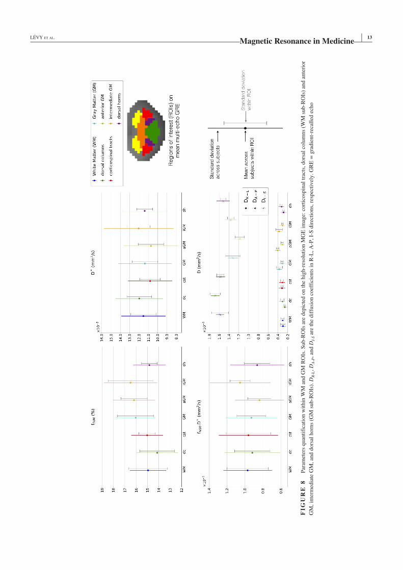
| 13LÉVY ET AL.

FI

GU

RE

8

Par

amet

ers

quan

tifi

cati

on w

ithin

WM

and G

M R

OIs

. S

ub-R

OIs

are

dep

icte

d o

n t

he

hig

h-r

esolu

tion M

GE

im

age:

cort

icosp

inal

tra

cts,

dors

al c

olu

mns

(WM

sub-R

OIs

) an

d a

nte

rior

GM

, in

term

edia

te G

M, an

d d

ors

al h

orn

s (G

M s

ub-R

OIs

). D

R-L

, D

A-P

, an

d D

I-S a

re t

he

dif

fusi

on c

oef

fici

ents

in R

-L, A

-P, I-

S d

irec

tions,

res

pec

tivel

y. G

RE

= g

radie

nt-

reca

lled

ech

o

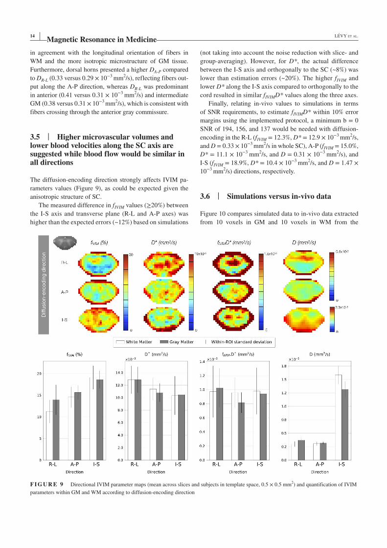
14 | LÉVY ET AL.

in agreement with the longitudinal orientation of fibers in

WM and the more isotropic microstructure of GM tissue.

Furthermore, dorsal horns presented a higher DA-P compared

to DR-L (0.33 versus 0.29 × 10−3 mm2/s), reflecting fibers out-

put along the A-P direction, whereas DR-L was predominant

in anterior (0.41 versus 0.31 × 10−3 mm2/s) and intermediate

GM (0.38 versus 0.31 × 10−3 mm2/s), which is consistent with

fibers crossing through the anterior gray commissure.

3.5 | Higher microvascular volumes and lower blood velocities along the SC axis are suggested while blood flow would be similar in all directions

The diffusion-encoding direction strongly affects IVIM pa-

rameters values (Figure 9), as could be expected given the

anisotropic structure of SC.

The measured difference in fIVIM values (≥20%) between

the I-S axis and transverse plane (R-L and A-P axes) was

higher than the expected errors (~12%) based on simulations

(not taking into account the noise reduction with slice- and

group-averaging). However, for D*, the actual difference

between the I-S axis and orthogonally to the SC (~8%) was

lower than estimation errors (~20%). The higher fIVIM and

lower D* along the I-S axis compared to orthogonally to the

cord resulted in similar fIVIMD* values along the three axes.

Finally, relating in-vivo values to simulations in terms

of SNR requirements, to estimate fIVIMD* within 10% error

margins using the implemented protocol, a minimum b = 0

SNR of 194, 156, and 137 would be needed with diffusion-

encoding in the R-L (fIVIM = 12.3%, D* = 12.9 × 10−3 mm2/s,

and D = 0.33 × 10−3 mm2/s in whole SC), A-P (fIVIM = 15.0%,

D* = 11.1 × 10−3 mm2/s, and D = 0.31 × 10−3 mm2/s), and

I-S (fIVIM = 18.9%, D* = 10.4 × 10−3 mm2/s, and D = 1.47 ×

10−3 mm2/s) directions, respectively.

3.6 | Simulations versus in-vivo data

Figure 10 compares simulated data to in-vivo data extracted

from 10 voxels in GM and 10 voxels in WM from the

F I G U R E 9 Directional IVIM parameter maps (mean across slices and subjects in template space, 0.5 × 0.5 mm2) and quantification of IVIM

parameters within GM and WM according to diffusion-encoding direction

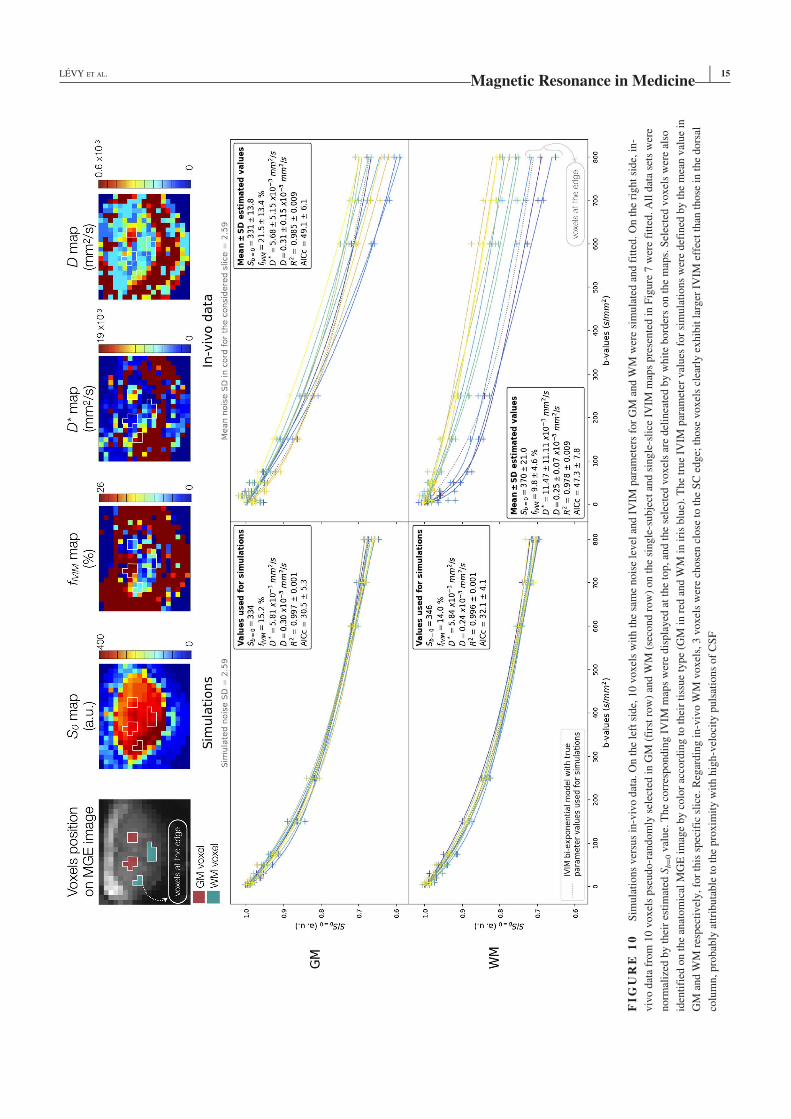
| 15LÉVY ET AL.

FI

GU

RE

10

S

imula

tions

ver

sus

in-v

ivo d

ata.

On t

he

left

sid

e, 1

0 v

oxel

s w

ith t

he

sam

e nois

e le

vel

and I

VIM

par

amet

ers

for

GM

and W

M w

ere

sim

ula

ted a

nd f

itte

d. O

n t

he

right

side,

in-

viv

o d

ata

from

10 v

oxel

s pse

udo-r

andom

ly s

elec

ted i

n G

M (

firs

t ro

w)

and W

M (

seco

nd r

ow

) on t

he

single

-subje

ct a

nd s

ingle

-sli

ce I

VIM

map

s pre

sente

d i

n F

igure

7 w

ere

fitt

ed. A

ll d

ata

sets

wer

e

norm

aliz

ed b

y t

hei

r es

tim

ated

Sb=

0 v

alue.

The

corr

espondin

g I

VIM

map

s w

ere

dis

pla

yed

at

the

top, an

d t

he

sele

cted

voxel

s ar

e del

inea

ted b

y w

hit

e bord

ers

on t

he

map

s. S

elec

ted v

oxel

s w

ere

also

iden

tifi

ed o

n t

he

anat

om

ical

MG

E i

mag

e by c

olo

r ac

cord

ing t

o t

hei

r ti

ssue

type

(GM

in r

ed a

nd W

M i

n i

ris

blu

e). T

he

true

IVIM

par

amet

er v

alues

for

sim

ula

tions

wer

e def

ined

by t

he

mea

n v

alue

in

GM

and W

M r

espec

tivel

y, fo

r th

is s

pec

ific

sli

ce. R

egar

din

g i

n-v

ivo W

M v

oxel

s, 3

voxel

s w

ere

chose

n c

lose

to t

he

SC

edge;

those

voxel

s cl

earl

y e

xhib

it l

arger

IV

IM e

ffec

t th

an t

hose

in t

he

dors

al

colu

mn, pro

bab

ly a

ttri

buta

ble

to t

he

pro

xim

ity w

ith h

igh-v

eloci

ty p

uls

atio

ns

of

CS

F

16 | LÉVY ET AL.

single-subject and single-slice maps presented in Figure 7.

Similar fit quality was observed between simulations and

in-vivo data (as evidenced by the coefficient of determination

R2), along with robust performances of the fitting algorithm.

However, signal decay profiles with b-value clearly differed

both between simulated and in-vivo data, but also between

voxels of a same tissue type for in-vivo data. In-vivo sig-

nal decay, as described by the current IVIM model, seems to

result from more than only the IVIM effect of capillary per-

fusion, suggesting potential confounding factors. This also

reflects in the Akaike Information Criterion corrected for

sample size (AICc), which is an index of the amount of infor-

mation lost by the model for the given data set.66 The AICc

was approximately 1.6 times higher for in-vivo data, support-

ing that in-vivo data included more information unexplained

by the IVIM model than synthetic data which were generated

from it. Finally, 3 WM in-vivo voxels stood out with a larger

IVIM effect; those voxels are at the edge of the SC and were

probably affected by the high-velocity pulsations of CSF.

Other WM voxels showed less IVIM effect than GM voxels,

as evidenced by the curve curvature.

4 | DISCUSSION

This work proposes a combined numerical and experimental

study for noninvasive perfusion imaging of the human cer-

vical SC using IVIM at 7T. Estimation errors and required

SNRs were first evaluated for expected in-vivo values. IVIM

maps were then derived at multiple averaging scales: from

single-subject and single-slice data to the total average. The

latter enabled to distinguish regional perfusion differences.

4.1 | Promises of IVIM imaging in the human SC

Although SNR within individual data were limited, averag-

ing maps across slices and subjects provided enough SNR to

highlight very small (1% of microvascular volume fraction)

regional perfusion differences between WM and GM, offer-

ing preliminary results of perfusion-related parameter map-

ping in the human SC in vivo.

In this first investigative study, mean values for fIVIM

and D* were 15.0% and 11.5 × 10−3 mm2/s in WM and

16.0% and 11.4 × 10−3 mm2/s in GM. Microvascular frac-

tion values were higher than the values of ~5% reported in

brain using positron emission tomography and 15O inhala-

tion method,67 but they are in the range of IVIM studies in

normal brain GM and WM26,27 even if the cohort explored

here needs to be extended. This potential overestimation

can be reduced by taking into account the relaxation rate

difference between blood and tissue in IVIM representation

as proposed by Lemke et al35; however, this was beyond the

scope of the current study. Regarding spatial distribution,

also in agreement with brain studies25,26,50 and anatomi-

cal charts,64 highest microvascular volumes (on average

maps) seem to match with GM location (mainly anterior

and intermediate GM). Moreover, the fIVIMD* map suggests

highest flow at the location of central arteries (Figure 7),

which represent the main blood supply to anterior horns.64

Average IVIM maps, and especially the microvascular vol-

ume fraction (fIVIM), also nicely compare with the microan-

giogram of transverse section of human SC at T6 level from

Hassler,65 even though SC structure varies from thoracic

to cervical levels. This microangiogram also illustrates the

difficulty to capture the SC perfusion levels from such a

sparse capillary network.

Whereas our findings stem from a single-center 7T

study, the protocol setup here can easily be translated to

different 7T human MR sites as well as to lower clinical

field with minor adaptation for potential clinical applica-

tions. Indeed, transferring the protocol to 3T could benefit

from lower B0 inhomogeneities, improved B1, and reduced

susceptibility effects, hence mitigating the lower theoreti-

cal SNR at this field.

Independent from field strength, our numerical evalua-

tion also showed that there is a crucial need for standardiza-

tion, and one potential asset is the growing availability of

open-source programs to encourage reproducible research.68

Fitting algorithms can significantly impact parameter estima-

tion errors. In particular, some optimization algorithms (e.g.,

Conjugate Gradient) showed little robustness to local optima

for some parameter sets with infinite SNR whereas others, such

as Differential Evolution48 (preferred here), systematically

provided the global optimum of the cost function. With the

objective to facilitate comparisons across studies and fitting

procedures, the programs used here were made open source

and available at: https ://github.com/slevy roset ti/ivim-toolbox.

We provide here the estimation errors associated with our

implementation, for given SNRs. Results also depend, to some

extent, on the b-value distribution, but trends are consistent

with those from Pekar et al,38 who used similar b-values.

However, given that literature in healthy WM and GM shows

variations as large as 13 × 10−3 mm2/s for D*39 and 13% for

fIVIM,26 the present work evaluated the full range of potential

IVIM values; and, indeed, results revealed a substantial varia-

tion in estimation accuracy within this range of values.

4.2 | Limitations and perspectives

One major limitation in the current setting is that single-

subject and single-slice IVIM maps were not reliable enough

to clearly discriminate between GM and WM perfusion.

Mean values across subjects (Figure 8) finally revealed

| 17LÉVY ET AL.

<10% perfusion difference in fIVIMD* between those 2 tis-

sues whereas the estimation error would be, at best, 9% with

the highest voxel-wise in-vivo measured SNRs (180), 13%

in average (120), and 27% at lowest SNRs (60). This poor

reliability in single-subject and single-slice maps makes the

protocol currently unsuitable for detecting locally restricted

abnormalities or for studying variations along the SC axis.

So far, the best precision for an individual diagnosis would

be the one obtained in slice-averaged maps. However, slice-

averaging would mitigate detection of locally restricted

abnormalities (e.g., existing on 1 slice only). Further devel-

opments are thus needed to reliably detect local perfusion

abnormalities or to study variations along the SC axis.

Furthermore, the theoretical required SNR was reached

in vivo for this study, but the method used to determine esti-

mation errors does not include inaccuracy of the IVIM biex-

ponential model, which is based on several assumptions (e.g.,

randomly oriented microvascular network, D* >> D, no ex-

change between intra- and extravascular compartments). The

comparison of simulated signal decay with b-value to in-vivo

profiles (Figure 10) suggests sources of bias in the model

that need to be addressed to improve estimation precision.

As demonstrated in Novikov et al,69 the biexponential model

is a signal representation very sensitive to biases. Potential

sources of bias could be microscopic nonlinear motion within

the cord or interstitial fluid adding IVIM effects independent

from tissue perfusion. The existence of different vessel func-

tional pools, as introduced by several researchers for IVIM

in the brain,70-73 could also be a source of bias. Besides, the

large slice thickness used in this study (5 mm) might mix

the different effects within each voxel in a complex man-

ner, adding to the inaccuracies. More sophisticated models

have shown better accuracy,74,75 but assessment of the IVIM

model was beyond the scope of this article.

Still, IVIM in the SC is highly SNR demanding, as ex-

pected, and the technique as used so far will hardly be able to

measure very low perfusion levels (e.g., fIVIM < 4% for diffu-

sion encoding in the SC transverse plane or fIVIM < 8% for dif-

fusion encoding along the SC axis) given the required SNRs

(>500) for single-subject and single-slice data. It should also

be noted that the IVIM technique is very sensitive to high

fluid velocities such as encountered within surrounding pul-

satile CSF. This is a non-negligible issue for voxels at the

edge of the SC, where signal is highly biased by partial vol-

ume effect with CSF, resulting in the high value ring that

can be observed on fIVIM, D*, and more extensively fIVIMD*

maps. Similarly, the central canal, which contains CSF, might

also be a source of bias in IVIM estimation within intermedi-

ate GM given that it can widen in some pathologies such as

syringomyelia.76 Fluid suppression strategies with inversion

recovery acquisition might be worth considering. Another

avenue would be to adjust the acquisition trigger delay to

subjects’ cardiac cycle given that the latter can vary across

populations, targeting the quiescent phase of both SC and

CSF motion. It might also be judicious to trigger the acquisi-

tion at the peak of perfusion flow given that fIVIMD* and D*

in the brain were shown to vary across the cardiac cycle.77

Moreover, this study reports errors and required SNRs for

healthy IVIM values, but perfusion levels might deviate in

pathological cases. In cases like gliomas, where perfusion in-

crease can go up by +30 × 10−3 mm2/s in D* and +10% in

fIVIM26,41,42 compared to healthy values, IVIM fitting errors

would be lowered down to 3% on fIVIMD* at SNR = 180. In

such cases, estimation would be precise enough to discrimi-

nate between healthy and pathological tissue. In contrast, in

ischemic strokes, fIVIM would be reduced by around –4%,28

corresponding to an error increase from 9% in healthy tis-

sue to around 20% in ischemic tissue, making ischemia

undetectable.

So far, the current acquisition protocol is too long to be

used in clinical routine and might be affected by additional

movements (e.g., swallowing) associated with patients’ dis-

comfort. Nonetheless, multiple avenues for improvement

exist. The b-value distribution and repetition numbers were

herein defined empirically; they can be optimized to reduce

scan time and/or improve parameter estimation. Monte-Carlo

simulations can be pushed further or the Cramer–Rao lower

bounds can also be used to this purpose.78 SNR increase

can be achieved through multiple ways. Improved hardware,

like more powerful gradients or design of more efficient

high-density coil arrays dedicated to ultrahigh field MRI,

will hopefully enable to reach higher SNR in shorter time.

Alternative k-space sampling schemes, such as spiral read-

out and inner FOV sequences, would reduce TE and distor-

tions associated with single-shot EPI. Finally, cutting-edge

fitting approaches might be worth considering. For instance,

Bayesian methods—which basically maximize the probabil-

ity density function of parameters—showed more robustness

to noise,79,80 but caution has to be taken given that fine per-

fusion variations could be smoothed when parameter uncer-

tainty is high.81

Nonetheless, the IVIM technique was able to provide us

with the first perfusion-related maps of the human spinal

cord in vivo without contrast agent injection, alleviating con-

cerns regarding the use of several gadolinium chelates.15,16 In

addition, along with perfusion information, IVIM provides

microstructural information from the diffusion coefficient,

which can be useful in the joint assessment of perfusion and

tissue integrity in the context of SC injuries.

5 | CONCLUSION

This study ultimately provides, to our knowledge, the first

perfusion-related maps of the human SC, paving the way

to in-vivo study of SC microvascularization processes, for

18 | LÉVY ET AL.

earlier diagnostic of perfusion abnormalities in a more dis-

tant future. Ultrahigh field MRI acquisition developments

and numerical simulations were combined to quantify IVIM

parameters and related estimation errors for representative

in-vivo SNRs. Although the technique did not show suffi-

cient reliability to achieve patient- and level-specific IVIM

mapping, the developed method provided preliminary results

of SC perfusion mapping, highlighting a very small perfu-

sion difference between GM and WM (~1% of microvascular

volume fraction) on group-averaged maps. Developments to

increase SNR, so as to reduce scan time and address potential

modeling biases, are warranted.

ACKNOWLEDGMENTS

The authors sincerely thank Ludovic de Rochefort, Olivier

Girard, and Sylviane Confort-Gouny for useful discussions,

Christophe Vilmen, Véronique Gimenez, Patrick Viout and

Lauriane Pini for the study logistics, as well as the Mesocenter

(Centre de Calcul Intensif) from Aix-Marseille University

for access to high performance computing resources.

This project received funding from the European Union’s

Horizon 2020 research and innovation program under the

Marie Skłodowska-Curie grant agreement #713750. Also, it

was carried out with the financial support of the Regional

Council of Provence-Alpes-Côte d’Azur and with the finan-

cial support of the A*MIDEX (#ANR-11-IDEX-0001-02),

funded by the Investissements d'Avenir project funded by

the French Government, managed by the French National

Research Agency (ANR).

This work was performed within a laboratory member of

France Life Imaging network (grant ANR-11-INBS-0006),

on the platform 7T-AMI, a French “Investissements d'Avenir”

programme (grant ANR-11-EQPX-0001). It received fund-

ings from the A*midex programme Excellence Inititative

of Aix-Marseille University (A*MIDEX-EI-13-07-130115-

08.38-7T-AMISTART) and from CNRS (Centre National de

la Recherche Scientifique).

ORCID

Simon Lévy https://orcid.org/0000-0002-6492-2990

Stanislas Rapacchi

https://orcid.org/0000-0002-8925-495X

Virginie Callot https://orcid.org/0000-0003-0850-1742

REFERENCES

1. Kolenda H, Steffens H, Gefeller O, Hagenah J, Schomburg E.

Critical levels of spinal cord blood flow and duration of ischemia

for the acute recovery of segmental spinal cord responses in cats.

J Spinal Disord. 1997;10:288–295.

2. Fehlings MG, Tetreault L, Hsieh PC, Traynelis V, Wang MY.

Introduction: degenerative cervical myelopathy: diagnostic, as-

sessment, and management strategies, surgical complications, and

outcome prediction. Neurosurg Focus. 2016;40:E1.

3. Vilaça CDO, Orsini M, Araujo Leite MA, et al. Cervical spondy-

lotic myelopathy: what the neurologist should know. Neurol Int.

2016;8:6330.

4. Martin AR, De Leener B, Cohen-Adad J, et al. Monitoring for

myelopathic progression with multiparametric quantitative MRI.

Toft M, ed. PLoS One. 2018;13:e0195733. https ://doi.org/10.1371/

journ al.pone.0195733.

5. Martin AR, Aleksanderek I, Cohen-Adad J, et al. Translating state-

of-the-art spinal cord MRI techniques to clinical use: a systematic

review of clinical studies utilizing DTI, MT, MWF, MRS, and

fMRI. Neuroimage Clin. 2016;10:192–238.

6. Fradet L, Arnoux PJ, Ranjeva JP, Petit Y, Callot V. Morphometrics

of the entire human spinal cord and spinal canal measured from

in vivo high-resolution anatomical magnetic resonance imaging.

Spine. 2014;39:E262–E269.

7. Figley CR, Stroman PW. Investigation of human cervical and upper

thoracic spinal cord motion: implications for imaging spinal cord

structure and function. Magn Reson Med. 2007;58:185–189.

8. Duhamel G, Callot V, Cozzone PJ, Kober F. Spinal cord blood

flow measurement by arterial spin labeling. Magn Reson Med.

2008;59:846–854.

9. Martirosian P, Klose U, Mader I, Schick F. FAIR true-FISP perfu-

sion imaging of the kidneys. Magn Reson Med. 2004;51:353–361.

10. Leporq B, Saint-Jalmes H, Rabrait C, et al. Optimization of in-

tra-voxel incoherent motion imaging at 3.0 Tesla for fast liver ex-

amination: Optimization of Liver Motion Imaging at 3.0T. J Magn

Reson Imaging. 2015;41:1209–1217.

11. Wang C, Han X, Jiang W, et al. Perfusion of spinal cord in post-

operative patient with cervical spondylotic myelopathy using MR

DSC technique. In Proceedings of the 25th Annual Meeting of

the International Society for Magnetic Resonance in Medicine,

Honolulu, HI, 2017. p. 2507.

12. Wang C, Han X, Jiang W, et al. Spinal cord perfusion is associ-

ated with diffusion and clinical mJOA score in preoperative pa-

tients with cervical spondylotic myelopathy. In Proceedings of the

26th Annual Meeting of the International Society for Magnetic

Resonance in Medicine, Paris, France, 2018. p. 5397.

13. Ellingson BM, Woodworth DC, Leu K, Salamon N, Holly LT.

Spinal cord perfusion MR imaging implicates both ischemia

and hypoxia in the pathogenesis of cervical spondylosis. World

Neurosurg. 2019;128:e773–e781.

14. Cuvinciuc V, Viallon M, Barnaure I, Vargas MI, Lovblad KO,

Haller S. Dynamic contrast-enhanced MR perfusion of intradural

spinal lesions. Am J Neuroradiol. 2017;38:192–194.

15. Ramalho J, Semelka RC, Ramalho M, Nunes RH, AlObaidy M,

Castillo M. Gadolinium-based contrast agent accumulation and

toxicity: an update. AJNR Am J Neuroradiol. 2016;37:1192–1198.

16. Kanda T, Fukusato T, Matsuda M, et al. Gadolinium-based con-

trast agent accumulates in the brain even in subjects without se-

vere renal dysfunction: evaluation of autopsy brain specimens

with inductively coupled plasma mass spectroscopy. Radiology.

2015;276:228–232.

17. Alsop DC, Detre JA, Golay X, et al. Recommended implementa-

tion of arterial spin-labeled perfusion MRI for clinical applications:

a consensus of the ISMRM perfusion study group and the European

consortium for ASL in dementia: Recommended Implementation of

ASL for Clinical Applications. Magn Reson Med. 2015;73:102–116.

18. Duhamel G, Callot V, Decherchi P, et al. Mouse lumbar and cervi-

cal spinal cord blood flow measurements by arterial spin labeling:

| 19LÉVY ET AL.

sensitivity optimization and first application. Magn Reson Med.

2009;62:430–439.

19. Girard OM, Callot V, Robert B, Cozzone PJ, Duhamel G. Perfusion

MRI of the human cervical spinal cord using arterial spin label-

ing. In Proceedings of the 21st Annual Meeting of the International

Society for Magnetic Resonance in Medicine, Salt Lake City, UT,

2013. p. 0349.

20. Nair G, Hu XP. Perfusion imaging of the human cervical spinal

cord. In Proceedings of the 19th Annual Meeting of the International

Society for Magnetic Resonance in Medicine, Stockholm, Sweden,

2010. p. 4083.

21. Wang YI, Moeller S, Li X, et al. Simultaneous multi-slice

turbo-FLASH imaging with CAIPIRINHA for whole brain

distortion-free pseudo-continuous arterial spin labeling at 3 and 7T.

Neuroimage. 2015;113:279–288.

22. Massire A, Taso M, Besson P, Guye M, Ranjeva JP, Callot V.

High-resolution multi-parametric quantitative magnetic resonance

imaging of the human cervical spinal cord at 7T. Neuroimage.

2016;143:58–69.

23. Massire A, Rasoanandrianina H, Taso M, et al. Feasibility

of single-shot multi-level multi-angle diffusion tensor imag-

ing of the human cervical spinal cord at 7T. Magn Reson Med.

2018;80:947–957.

24. Le Bihan D, Breton E, Lallemand D, Aubin ML, Vignaud J, Laval-

Jeantet M. Separation of diffusion and perfusion in intravoxel inco-

herent motion MR imaging. Radiology. 1988;168:497–505.

25. Wang C, Ren D, Guo Y, et al. Distribution of intravoxel incoher-

ent motion MRI-related parameters in the brain: evidence of inter-

hemispheric asymmetry. Clin Radiol. 2017;72:94.e1–94.e6.

26. Bisdas S, Klose U. IVIM analysis of brain tumors: an investigation

of the relaxation effects of CSF, blood, and tumor tissue on the

estimated perfusion fraction. Magn Reson Mater Phys Biol Med.

2015;28:377–383.

27. Bertleff M, Domsch S, Weingärtner S, et al. Diffusion parameter

mapping with the combined intravoxel incoherent motion and kur-

tosis model using artificial neural networks at 3 T. NMR Biomed.

2017;30:e3833.

28. Suo S, Cao M, Zhu W, et al. Stroke assessment with intravoxel

incoherent motion diffusion-weighted MRI. NMR Biomed.

2016;29:320–328.

29. Federau C. Intravoxel incoherent motion MRI as a means to mea-

sure in vivo perfusion: A review of the evidence. NMR Biomed.

2017;30:e3780.

30. Maximov II, Vellmer S. Isotropically weighted intravoxel in-

coherent motion brain imaging at 7T. Magn Reson Imaging.

2019;57:124–132.

31. Milani B, Ledoux JB, Rotzinger DC, et al. Image acquisition for

intravoxel incoherent motion imaging of kidneys should be trig-

gered at the instant of maximum blood velocity: evidence obtained

with simulations and in vivo experiments. Magn Reson Med.

2019;81:583–593.

32. Gambarota G, Hitti E, Leporq B, Saint-Jalmes H, Beuf O.

Eliminating the blood-flow confounding effect in intravoxel inco-

herent motion (IVIM) using the non-negative least square analysis

in liver: NNLS analysis of IVIM data in liver. Magn Reson Med.

2017;77:310–317.

33. Jalnefjord O, Andersson M, Montelius M, et al. Comparison of

methods for estimation of the intravoxel incoherent motion (IVIM)

diffusion coefficient (D) and perfusion fraction (f). MAGMA.

2018;31:715–723.

34. Xiang Z, Ai Z, Liang J, Li G, Zhu X, Yan X. Evaluation of re-

gional variability and measurement reproducibility of intravoxel

incoherent motion diffusion weighted imaging using a cardiac

stationary phase based ECG trigger method. BioMed Res Int.

2018;2018:4604218.

35. Lemke A, Laun FB, Simon D, Stieltjes B, Schad LR. An in vivo

verification of the intravoxel incoherent motion effect in dif-

fusion-weighted imaging of the abdomen. Magn Reson Med.

2010;64:1580–1585.

36. Barbieri S, Donati OF, Froehlich JM, Thoeny HC. Impact of

the calculation algorithm on biexponential fitting of diffu-

sion-weighted MRI in upper abdominal organs. Magn Reson Med.

2016;75:2175–2184.

37. Gurney-Champion OJ, Klaassen R, Froeling M, et al. Comparison

of six fit algorithms for the intra-voxel incoherent motion model of

diffusion-weighted magnetic resonance imaging data of pancreatic

cancer patients. PLoS One. 2018;13:e0194590.

38. Pekar J, Moonen CT, van Zijl PC. On the precision of diffusion/

perfusion imaging by gradient sensitization. Magn Reson Med.

1992;23:122–129.

39. Federau C, O’Brien K, Meuli R, Hagmann P, Maeder P.

Measuring brain perfusion with intravoxel incoherent motion

(IVIM): initial clinical experience. J Magn Reson Imaging.

2014;39:624–632.

40. Federau C, Maeder P, O’Brien K, Browaeys P, Meuli R, Hagmann

P. Quantitative measurement of brain perfusion with intravoxel in-

coherent motion MR imaging. Radiology. 2012;265:874–881.

41. Bisdas S, Koh TS, Roder C, et al. Intravoxel incoherent motion dif-

fusion-weighted MR imaging of gliomas: feasibility of the method

and initial results. Neuroradiology. 2013;55:1189–1196.

42. Federau C, Meuli R, O’Brien K, Maeder P, Hagmann P. Perfusion

measurement in brain gliomas with intravoxel incoherent motion

MRI. Am J Neuroradiol. 2014;35:256–262.

43. Taso M, Girard OM, Duhamel G, et al. Tract-specific and age-

related variations of the spinal cord microstructure: a multi-

parametric MRI study using diffusion tensor imaging (DTI) and

inhomogeneous magnetization transfer (ihMT). NMR Biomed.

2016;29:817–832.

44. Finkenstaedt T, Klarhoefer M, Eberhardt C, et al. The IVIM sig-

nal in the healthy cerebral gray matter: a play of spherical and

non-spherical components. Neuroimage. 2017;152:340–347.

45. Samson RS, Lévy S, Schneider T, et al. ZOOM or Non-ZOOM?

assessing spinal cord diffusion tensor imaging protocols for

multi-centre studies. PLoS One. 2016;11:e0155557.

46. Xu J, Shimony JS, Klawiter EC, et al. Improved in vivo diffu-

sion tensor imaging of human cervical spinal cord. Neuroimage.

2013;67:64–76.

47. Bihan DL, Turner R. The capillary network: a link between IVIM

and classical perfusion. Magn Reson Med. 1992;27:171–178.

48. Storn R, Price K. Differential evolution—a simple and efficient

heuristic for global optimization over continuous spaces. J Glob

Optim. 1997;11:341–359.

49. Vonken EJ, van Osch MJ, Bakker CJ, Viergever MA. Measurement

of cerebral perfusion with dual-echo multi-slice quantitative

dynamic susceptibility contrast MRI. J Magn Reson Imaging.

1999;10:109–117.

50. Parkes LM, Waqar R, Chard DT, Tofts PS. Normal cerebral

perfusion measurements using arterial spin labeling: reproduc-

ibility, stability, and age and gender effects. Magn Reson Med.

2004;51:736–743.

20 | LÉVY ET AL.

51. Morelli JN, Runge VM, Feiweier T, Kirsch JE, Williams KW,

Attenberger UI. Evaluation of a modified Stejskal-Tanner diffu-

sion encoding scheme, permitting a marked reduction in TE, in

diffusion-weighted imaging of stroke patients at 3 T. Invest Radiol.

2010;45:29–35.

52. DiIorio G, Brown JJ, Borrello JA, Perman WH, Shu HH. Large

angle spin-echo imaging. Magn Reson Imaging. 1995;13:39–44.

53. Alley S, Gilbert G, Gandini Wheeler-Kingshott C, et al. Consensus

acquisition protocol for quantitative MRI of the cervical spinal

cord at 3T. In Proceedings of the 26th Annual Meeting of the

International Society for Magnetic Resonance in Medicine, Paris,

France, 2018. p. 0799.

54. Manjón JV, Coupé P, Concha L, Buades A, Collins DL, Robles

M. Diffusion weighted image denoising using overcomplete local

PCA. PLoS One. 2013;8:e73021.

55. Kellner E, Dhital B, Kiselev VG, Reisert M. Gibbs-ringing arti-

fact removal based on local subvoxel-shifts. Magn Reson Med.

2016;76:1574–1581.

56. De Leener B, Lévy S, Dupont SM, et al. SCT: Spinal Cord

Toolbox, an open-source software for processing spinal cord MRI

data. Neuroimage. 2017;145:24–43.

57. Andersson JL, Skare S, Ashburner J. How to correct susceptibility

distortions in spin-echo echo-planar images: application to diffu-

sion tensor imaging. Neuroimage. 2003;20:870–888.

58. Reeder SB, Wintersperger BJ, Dietrich O, et al. Practical ap-

proaches to the evaluation of signal-to-noise ratio performance

with parallel imaging: application with cardiac imaging and a

32-channel cardiac coil. Magn Reson Med. 2005;54:748–754.

59. De Leener B, Fonov VS, Collins DL, Callot V, Stikov N, Cohen-

Adad J. PAM50: unbiased multimodal template of the brainstem

and spinal cord aligned with the ICBM152 space. Neuroimage.

2018;165:170–179.

60. Lévy S, Benhamou M, Naaman C, Rainville P, Callot V, Cohen-

Adad J. White matter atlas of the human spinal cord with estima-

tion of partial volume effect. Neuroimage. 2015;119:262–271.

61. De Leener B, Kadoury S, Cohen-Adad J. Robust, accurate and

fast automatic segmentation of the spinal cord. Neuroimage.

2014;98:528–536.

62. Perone CS, Calabrese E, Cohen-Adad J. Spinal cord gray matter seg-

mentation using deep dilated convolutions. Sci Rep. 2018;8:5966.

63. Gillilan LA. The arterial blood supply of the human spinal cord.

J Comp Neurol. 1958;110:75–103.

64. Martirosyan NL, Feuerstein JS, Theodore N, Cavalcanti DD,

Spetzler RF, Preul MC. Blood supply and vascular reactivity of

the spinal cord under normal and pathological conditions: a review.

J Neurosurg Spine. 2011;15:238–251.

65. Hassler O. Blood supply to human spinal cord: a microangio-

graphic study. Arch Neurol. 1966;15:302–307.

66. Akaike H. A new look at the statistical model identification. IEEE

Trans Autom Control. 1974;19:716–723.

67. Leenders KL, Perani D, Lammertsma AA, et al. Cerebral blood

flow, blood volume and oxygen utilization: normal values and ef-

fect of age. Brain. 1990;113:27–47.

68. Stikov N, Trzasko JD, Bernstein MA. Reproducibility and the fu-

ture of MRI research. Magn Reson Med. 2019;82:1981–1983.

69. Novikov DS, Kiselev VG, Jespersen SN. On modeling. Magn

Reson Med. 2018;79:3172–3193.

70. Kennan RP, Gao JH, Zhong J, Gore JC. A general model of mi-

crocirculatory blood flow effects in gradient sensitized MRI. Med

Phys. 1994;21:539–545.

71. Henkelman RM, Neil JJ, Xiang QS. A quantitative interpretation

of IVIM measurements of vascular perfusion in the rat brain.

Magn Reson Med. 1994;32:464–469.

72. Duong TQ, Kim SG. In vivo MR measurements of regional arterial

and venous blood volume fractions in intact rat brain. Magn Reson

Med. 2000;43:393–402.

73. Fournet G, Li JR, Cerjanic AM, Sutton BP, Ciobanu L, Le Bihan

D. A two-pool model to describe the IVIM cerebral perfusion.

J Cereb Blood Flow Metab. 2017;37:2987–3000.

74. Wetscherek A, Stieltjes B, Laun FB. Flow-compensated intra-

voxel incoherent motion diffusion imaging. Magn Reson Med.

2015;74:410–419.

75. Schneider MJ, Gaass T, Ricke J, Dinkel J, Dietrich O. Assessment

of intravoxel incoherent motion MRI with an artificial capillary

network: analysis of biexponential and phase-distribution models.

Magn Reson Med. 2019;82:1373–1384.

76. Gardner WJ. Hydrodynamic mechanism of syringomyelia:

its relationship to myelocele. J Neurol Neurosurg Psychiatry.

1965;28:247–259.

77. Federau C, Hagmann P, Maeder P, et al. Dependence of brain intra-

voxel incoherent motion perfusion parameters on the cardiac cycle.

Hendrikse J, ed. PLoS One. 2013;8:e72856.

78. Jalnefjord O, Montelius M, Starck G, Ljungberg M. Optimization

of b-value schemes for estimation of the diffusion coefficient and

the perfusion fraction with segmented intravoxel incoherent mo-

tion model fitting. Magn Reson Med. 2019;82:1541–1552.

79. Neil JJ, Bretthorst GL. On the use of bayesian probability theory

for analysis of exponential decay date: an example taken from

intravoxel incoherent motion experiments. Magn Reson Med.

1993;29:642–647.

80. Ye C, Xu D, Qin Y, et al. Estimation of intravoxel incoherent motion

parameters using low b-values. PLoS One. 2019;14:e0211911.

81. While PT. A comparative simulation study of bayesian fitting

approaches to intravoxel incoherent motion modeling in diffu-

sion-weighted MRI: Bayesian fitting approaches to IVIM model-

ing in DWI. Magn Reson Med. 2017;78:2373–2387.

SUPPORTING INFORMATION

Additional supporting information may be found online in

the Supporting Information section.

FIGURE S1 Experimental optimization of acquisition

parameters

FIGURE S2 Comparison of IVIM fitting approaches for the

human spinal cord: the two-step segmented approach versus

the one-step approach

FIGURE S3 In vivo SNR distribution within spinal cord for

the cohort studied

TABLE S1 Acquisition protocol

How to cite this article: Lévy S, Rapacchi S,

Massire A, et al. Intravoxel Incoherent Motion at

7 Tesla to quantify human spinal cord perfusion:

Limitations and promises. Magn Reson Med.

2020;00:1–20. https ://doi.org/10.1002/mrm.28195

4.3 Concluding remarks

Although IVIM in the human spinal cord at 7T did not show sufficient reliability to map

perfusion at the single-subject and single-slice averaging scale and to potentially be used

in a clinical context, there is still room for improvements. In particular, the acquisition

time and/or the reliability could be improve with an optimized distribution of b-values

and number of repetitions by b-value, as mentioned in the article and further described in

section section 7.1.5. Such investigations have been initiated as part of this thesis using

the computational resources provided by Aix-Marseille University Mesocenter. Another

avenue for improvement is the inner field-of-view acquisition strategies making use of

selective two-dimensional RF pulses to excite a tight field-of-view around the cord in 2D

transversal slices only, and allowing a high-resolution with a reduced acquisition matrix.

The developed IVIM protocol has been tested with such sequence at 3T in collaboration

with the group of Patrick Freund at the Spinal Cord Injury Center of Balgrist University

Hospital in Zurich. The promising Signal-to-Noise Ratio results obtained suggested a

possible transfer of the technique to 3T or an increased reliability and/or a reduced

acquisition time with such technology at 7T.

142 Chapter 4

https://mesocentre.univ-amu.fr/

Feasibility of human spinal cord

perfusion mapping using

Dynamic Susceptibility Contrast

imaging at 7T: preliminary

results and identified guidelines

5

5.1 Foreword

This chapter is dedicated to the second article resulting from this thesis and accepted

for publication in the journal Magnetic Resonance in Medicine on September 23, 2020.

Given the poor reliability of Intra-Voxel Incoherent Motion (IVIM) maps at the individ-

ual and slice averaging level, the increased sensitivity provided by exogenous contrast

agents with the Dynamic Susceptibility Contrast (DSC) technique has then been investi-

gated at 7T. In this work, sequence developments and optimizations were first conducted

to set up an appropriate acquisition protocol for perfusion mapping with cardiac trigger-

ing and limited signal drop outs, both using spin-echo and gradient-echo EPI sequences.

In particular, the effects of respiration on signal steadiness were quantified. An image and

signal processing pipeline was set up to address the identified sources of instability. At a

second stage, data were acquired with the developed protocols in three healthy volunteers

and five Degenerative Cervical Myelopathy (DCM) patients (including one before and

after decompression surgery) who were recruited thanks to Pr. Pierre-Hugues Roche,

head of the Neurosurgery department at Hôpital Nord in Marseille. Obtained perfusion

maps successfully identified the higher gray matter perfusion in healhty volunteers but

results were mitigated in patients. Nonetheless, DSC appeared as a better candidate for

perfusion mapping of the human spinal cord in a clinical context, despite the involvement

of an exogenous contrast agent injection.

This work will be presented at the session entitled « Spinal Cord: Anatomy, Acquisition

& Assessment of Abnormalities » during the 2020 ISMRM Annual Meeting.

143

5.2 Manuscript

Title:

Feasibility of human spinal cord perfusion mappingusing Dynamic Susceptibility Contrast imaging at 7T:

preliminary results and identified guidelines

Authors:

Simon Lévya,b,c,d, Pierre-Hugues Roched,e, Maxime Guyea,b, Virginie Callota,b,d

Affiliations:a Aix-Marseille Univ, CNRS, CRMBM, Marseille, Franceb APHM, Hopital Universitaire Timone, CEMEREM, Marseille, Francec Aix-Marseille Univ, Univ Gustave Eiffel, LBA, Marseille, Franced iLab-Spine International Associated Laboratory, Marseille-Montreal, France-Canadae APHM, Hopital Nord, Neurosurgery Department, Marseille, France

Journal:

Submitted on July 24, 2020 to Magnetic Resonance in Medicine

Abstract

Purpose: To explore the feasibility of Dy-

namic Susceptibility Contrast (DSC) MRI at

7T for human spinal cord (SC) perfusion

mapping and fill the gap between brain and

SC cord perfusion mapping techniques.

Methods: Acquisition protocols for high-

resolution single-shot EPI in the SC were

optimized for both spin-echo and gradient-

echo preparations, including cardiac gat-

ing, acquisition times and breathing cycle

recording. Breathing-induced MRI signal

fluctuations were investigated in healthy

volunteers. A specific image and signal pro-

cessing pipeline was implemented to ad-

dress them.

The DSC technique was then evaluated in

3 healthy volunteers and 5 cervical spondy-

lotic myelopathy patients. Bolus depiction

on slice-wise signal within cord was investi-

gated and maps of relative perfusion indices

were computed.

Results: Signal fluctuations were divided

by 1.9 and 2.3 in apnea compared to free

breathing with spin-echo and gradient-echo,

144 Chapter 5

respectively. The ratio between signal fluc-

tuations and bolus peak in healthy volun-

teers was 5.0 % for spin-echo and 3.8 % for

gradient-echo, allowing a clear depiction of

the bolus on every slice and yielding rela-

tive blood flow and volume maps exhibiting

the expected higher perfusion of gray mat-

ter.

However, in patients, signal fluctuations

were increased by 4 in average using spin-

echo, compromising the depiction of the

bolus on slice-wise signal. Moreover, 3/18

slices had to be discarded because of fat

aliasing artifacts.

Conclusion: DSC MRI at 7T showed great

potential for SC perfusion mapping with

results never achieved so far for single-

subject and single-slice measurements. Sig-

nal stability needs to be improved in acquisi-

tion conditions associated with patients, but

guidelines to achieve that were identified

and proposed.

Keywords: spinal cord, dynamic suscepti-

bility contrast, DSC MRI, 7T MRI, perfusion,

ultrahigh field MRI

Introduction

Blood perfusion is frequently involved in

spinal cord (SC) injuries (Schubert, 2017;

Gilmor et al., 1998). Indeed, a prolonged

SC compression such as in traumas may

result in a local reduction of tissue perfu-

sion and progressive ischemia, leading to

metabolism alteration and potentially irre-

versible tissue necrosis (Beattie et al., 2000).

In such case, perfusion recovery is condi-

tional to clinical presentation improvement.

Similarly, in non-traumatic disorders such

as Cervical Spondylotic Myelopathy (CSM),

chronic SC compression may progressively

induce ischemia (Kalsi-Ryan et al., 2012).

Unfortunately today, there is a critical lack

of technique to confidently assess SC perfu-

sion status.

By contrast, in the brain, several tech-

niques such as Arterial Spin Labeling (ASL)

(Alsop et al., 2015), Intra-Voxel Incoherent

Motion (IVIM) (Le Bihan et al., 1988) or

the reference technique in clinics, Dynamic

Susceptibility Contrast (DSC) MRI, can now

provide reliable blood volume and blood

flow maps of patients with white (WM) and

gray (GM) matter distinction. Such maps

are an important tool for clinicians to assess

the extent of ischemic stroke for instance

(Aracki-Trenkic et al., 2020). From a clini-

cal point of view, SC perfusion maps would

be valuable to assess the extent and pro-

gression of perfusion deficit and identify

the specific functional area at stake. From

a technical point of view, regional mapping

of SC perfusion with high resolution would

also be a way to assess the reliability of the

measurements. Indeed, a similar GM/WM

perfusion difference in brain and SC is ex-

pected (based on microangiography (Turn-

bull, 1973), histology (Tator et al., 1997)

and ASL in mice (Duhamel et al., 2008)).

However, the transfer of the techniques

5.2 Manuscript 145

used in brain to SC is not trivial. Indeed,

its location in the vicinity of lungs, directly

surrounded by pulsatile Cerebrospinal Fluid

(CSF), is source of multiple biases and arti-

facts. In particular, breathing-induced field

fluctuations have shown a significant effect

on MRI signal, even at the cervical level

(Verma et al., 2014; Vannesjo et al., 2018).

Moreover, its size (∼8×13 mm2 in trans-

verse section) requires high resolution to

allow GM depiction. An additional chal-

lenge, similar to the brain (Duhamel et al.,

2008; Lu et al., 2008), is the low perfu-

sion level compared to other organs (e.g.

kidneys, liver, heart), with GM being more

perfused than WM (Duhamel et al., 2008;

Parkes Laura M. et al., 2004).

Among endogenous methods, ASL has

been experimented at 1.5T (Girard et al.,

2013) and 3T (Nair et al., 2010) for SC per-

fusion mapping. However, only poor sensi-

tivity and reliability were obtained. IVIM

was evaluated at 7T, but sensitivity at single-

subject and single-slice scale was limited

and averaging across multiple subjects (≥6)

was necessary to map the perfusion differ-

ence between GM and WM (Lévy et al.,

2020).

Using gadolinium injection, Vascular-

Space-Occupancy (VASO) MRI has been

used to map the absolute SC blood vol-

ume (BV) in healthy subjects (Lu et al.,

2008). A mean value of 4.3 mL/100 mL tis-

sue was obtained with a good reproducibil-

ity across field strengths (1.5 and 3T). How-

ever, this technique does not provide blood

flow-relative metrics. In addition, inflow-

ing fresh blood (Donahue et al., 2009) and

CSF volume changes (Scouten et al., 2008)

were shown to affect VASO MRI measure-

ments. Later, DSC was employed in CSM pa-

tients where ischemia is expected (Fehlings

et al., 1998), and showed promising sen-

sitivity at 3T. Indeed, relative SC BV was

negatively correlated to cord compression

and decreased with symptoms severity as

assessed by clinical tests (Ellingson et al.,

2019). However, those results were ob-

tained at the group level through multiple

voxel- and slice-averaged perfusion mea-

surements, with coarse resolution, which

helped sensitivity but excluded individual

and regional perfusion mapping, limiting

the clinical impact. In this exploratory study,

we aimed to assess the potential of DSC MRI

for regional perfusion-related indices map-

ping at the individual scale.

To cope with the high-resolution neces-

sary to GM and WM imaging in SC, the

investigations were performed at 7T, which

is now becoming a clinical tool (Staff News

Brief, 2017; Polimeni et al., 2018; Kraff

et al., 2017). Higher field strength theo-

retically provides higher SNR but also in-

creases susceptibility effects, which is ex-

pected to provide an increased sensitiv-

ity to gadolinium-based contrast agent bo-

lus in DSC imaging (Rohrer et al., 2005;

Noebauer-Huhmann et al., 2008). How-

ever, higher field strength also comes with

new challenges. Sensitivity to susceptibil-

ity variations and resulting B0 inhomogene-

146 Chapter 5

ity/fluctuations is increased. B1 transmis-

sion (B1+) and reception (B1-) are more

limited and heterogeneous. Such features

have significant consequences in the SC

physiological environment. The feasibility

and sensitivity of DSC MRI at 7T for hu-

man spinal cord perfusion mapping were

therefore investigated.

Materials and Methods

All acquisitions were performed on a 7T

whole-body research system (Magnetom,

Siemens Healthcare, Erlangen, Germany)

using a commercial 8-channel cervical-spine

transceiver surface coil (Rapid Biomedical

GmbH, Rimpar, Germany) with the 8 Tx-

channels hardware-combined into a single

transmit system.

Acquisition parameters

Acquisitions were cardiac gated (pulse

oximeter) to mitigate cord motion with CSF

pulsations. A single-shot two-dimensional

EPI readout was employed given the high

temporal resolution required, determined

by the cardiac beat. Physiological Moni-

toring Unit (PMU) was activated in the se-

quence code to allow acquisition time stamp

recordings, further used for post-processing

normalization by effective TR. A respiratory

belt was placed either on the subject’s ab-

domen or chest (depending on her/his main

mode of breathing) to record breathing cy-

cles during acquisition.

DSC can be performed using either

gradient-echo sequence based on the

change ∆R2∗ in R2

∗ relaxation rate, or spin-

echo sequence looking at the change ∆R2

in R2 relaxation rate. Both types of se-

quences were investigated.

An in-plane resolution of 0.7×0.7mm2

was aimed for, which was obtained with

truncated FOV coming with aliasing at the

edges but far from the cord. Acquisitions

were also performed with a coarser reso-

lution (1.0×1.0mm2) allowing the FOV to

include the whole neck cross-section. Fat

saturation was used without outer volume

suppression. Slice thickness was set to 5mm.

An acceleration factor of 2 (GRAPPA) was

used. Automatic calibration scans, partial

Fourier and TE were single-shot EPI, 6/8

and 42ms for the spin-echo sequence, and

gradient-echo FLASH, 5/8 and 22ms for the

gradient-echo sequence, respectively.

Acquisitions so far were limited to 3

slices (one by vertebral level, see Figure 5.1)

because of the Specific-Absorption-Rate

(SAR) restrictions associated with spin-echo

and TR around 800-1100 ms (cardiac cy-

cle). To optimize SNR with regards to the

subject’s cardiac cycle (effective TR), when

allowed by SAR limits, excitation flip angle

was set to the corresponding Ernst angle

(or 180 – Ernst angle for spin-echo), with

TR being the mean cardiac cycle duration

and T1 the mean longitudinal relaxation in

healthy SC tissue at 7T (∼1251 ms (Massire

et al., 2016)).

5.2 Manuscript 147

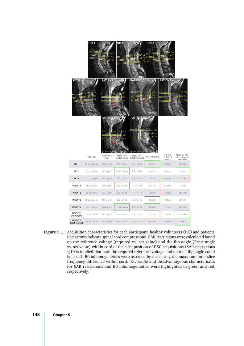
C3

C5

C4

Age / SexBody Mass

Index

Mean ± SD

cardiac period

Mean ± SD

breathing periodSAR restrictions

Shortest

cord<>coil

distance

Maximum inter-

slice frequency

difference

HC 1 37 y.o. / Female 18.93 kg/m2 903 ± 67 ms 4.1 ± 0.66 s 3.70 % 4.23 cm 63.8 Hz

HC 2 32 y.o. / Male 24.77 kg/m2 1064 ± 56 ms 2.9 ± 0.49 s 15.31 % 5.32 cm 17.4 Hz

HC 3 33 y.o. / Male 24.57 kg/m2 900 ± 54 ms 4.0 ± 0.52 s 2.45 % 4.44 cm 63.9 Hz

PATIENT 1 56 y.o. / Male 25.80 kg/m2 865 ± 38 ms 3.5 ± 0.48 s 61.41 % 5.34 cm 47.8 Hz


PATIENT 3 58 y.o. / Female 24.61 kg/m2 900 ± 34 ms 4.8 ± 0.71 s 10.63 % 4.34 cm 32.3 Hz


PATIENT 5

(pre-surgery)54 y.o. / Male 24.11 kg/m2 901 ± 31 ms 4.4 ± 1.43 s 55.42 % 5.40 cm 10.4 Hz

PATIENT 5

(post-surgery)55 y.o. / Male 27.44 kg/m2 952 ± 68 ms 5.0 ± 2.04 s 18.25 % 4.35 cm 7.6 Hz

C2

C3

C4

C2

C3

C4

C3

C5

C4

C2C3

C4

C2

C3

C4

C2

C4

C3

C2

C4

C3C2

C3

C4

HC 1 HC 2 HC 3

PATIENT 1 PATIENT 2 PATIENT 3 PATIENT 4

PATIENT 5 PATIENT 5

(pre-surgery) (post-surgery)

Figure 5.1.: Acquisition characteristics for each participant, healthy volunteers (HC) and patients.Red arrows indicate spinal cord compressions. SAR restrictions were calculated basedon the reference voltage (required vs. set value) and the flip angle (Ernst anglevs. set value) within cord at the slice position of DSC acquisitions (SAR restrictions≤10 % implied that both the required reference voltage and optimal flip angle couldbe used). B0 inhomogeneities were assessed by measuring the maximum inter-slicefrequency difference within cord. Favorable and disadvantageous characteristicsfor SAR restrictions and B0 inhomogeneities were highlighted in green and red,respectively.

148 Chapter 5

In-vivo evaluation

The study was approved by the local

ethics committee and written consents were

obtained from all participants prior to MR

examinations.

First, the effects of breathing on sig-

nal stability were investigated within 5

healthy volunteers (2 with spin-echo, 2 with

gradient-echo and 1 with both sequences).

Inspired apnea was asked to the partici-

pant at the beginning of acquisition. Data

were compared with free breathing condi-

tion and the temporal standard-deviation

(tSD) of ∆R2(∗) (∆R2 for spin-echo, ∆R∗

2

for gradient-echo) was used to quantify sig-

nal stability.

Then, 3 healthy volunteers and 5 pa-

tients with CSM were recruited for eval-

uation of the technique with gadolinium

injection. Each participant’s characteristics

are presented in Figure 5.1. One of the pa-

tients was scanned before and after decom-

pression surgery. The acquisition protocol

included:

• B1+ map: sagittal 2D saturation-

prepared turbo-flash with 1.0×1.0 mm2

in-plane resolution, 5 mm slice-thickness

• Sagittal anatomical imaging to refine

slice position: 2D turbo spin-echo with

0.6×0. 6mm2 in-plane resolution, 2.2 mm

slice thickness

• B0 map: sagittal 2D spoiled gradient-

echo with 1.35×1.35 mm2 in-plane reso-

lution, 5 mm slice-thickness

• Transversal anatomical imaging for

WM/GM depiction: 2D multi-echo

gradient-echo FLASH images with

0.4×0.4mm2 in-plane resolution, 5 mm

slice-thickness, same slice position as for

perfusion imaging.

• Perfusion imaging:

– DSC sequence (without injection)

with reverse (left>right) phase-

encoding direction (further used

for post-processing distortion correc-

tion), 100 repetitions (time points).

– DSC sequence with forward

(right>left) phase-encoding direc-

tion, 220 repetitions, with injection

after 70 repetitions (Dotarem, Guer-

bet, 0.2 mL/kg, 5 mL/s, followed by

30 mL saline flush).

Acquisition time for perfusion imag-

ing was ∼4 minutes depending on the

subject’s heartbeat, while the complete

protocol lasted ∼35 minutes. Shimming

for perfusion imaging was performed in a

rectangular box, positioned longitudinally

to the cord (∼4×3×9 cm3 along Right-

Left×Anterior-Posterior×Inferior-Superior

axes). A full-width-at-half-maximum

≤100Hz and T2∗ ≥5ms were targeted.

Data post-processing

The following image processing pipeline

was set up for DSC data:

5.2 Manuscript 149

1) Gibbs artefacts were removed using

the sub-pixel shifting method (Kellner

et al., 2016) (only for high-resolution

acquisitions).

2) A rigid motion correction was applied

slice-by-slice across repetitions using

ANTs (Avants et al., 2011) with the ac-

cumulated mean across registered im-

ages as reference (starting from first

repetition).

3) Denoising was applied with nonlocal

transform-domain filter (Maggioni et

al., 2013) (only for high-resolution

acquisitions).

Steps 1 to 3 were applied to both reversed

and forward phase-encoded series.

4) Distortion correction was applied

with Topup (Andersson et al., 2003)

based on the temporal mean of the

reversed and forward phase-encoded

series.

Then, a specific signal processing

pipeline was implemented in Python 3.6

as described below. The effects of each step

can be observed in Figure 5.2.

5) Effective TR normalization: point-

wise division by 1 − e−T Reff /T1 with

TReff the effective TR retrieved from

the PMU and T1 the average T1 value

in SC at 7T (Massire et al., 2016).

6) Discard inconsistent TRs: data ac-

quired after a missed trigger and the

following repetition were discarded

from analysis because of steady-state

loss (the first two repetitions were

therefore also discarded).

7) Breathing frequencies filtering: a

band-stop filter (Butterworth) was

applied using the minimum and maxi-

mum breathing frequencies measured

with the respiratory belt as cut-offs.

8) Final smoothing: a Savitzky-Golay fil-

ter with window length of 23 and

a 5th-order polynomial was applied.

Special care was taken not to smooth

out the bolus peak. This parameter

set yielded a good trade-off between

smoothing of residual signal oscilla-

tions and bolus conservation for all

subjects.

Data quality assessment

Native image series (both with forward

and reverse phase encoding) were visu-

ally inspected in comparison to transver-

sal anatomical multi-echo gradient-echo

FLASH images to assess image distortion

and spot any artifacts. Artifacts frequently

encountered in high-resolution EPI of the

SC — namely Nyquist N/2 ghosting, large

signal dropout (mainly with gradient-echo

sequences) or fat aliasing — are illustrated

in Figure 5.3. Slices with artifacts reaching

the cord were discarded.

150 Chapter 5

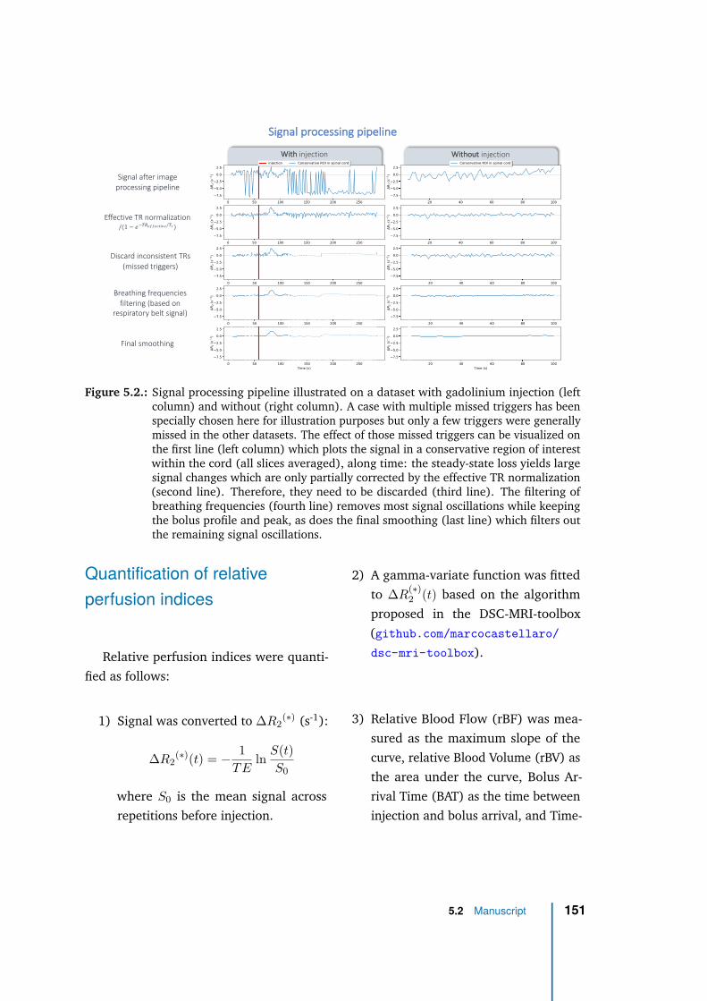
Without injectionWith injection

Effective TR normalization/(1 − 𝑒 ⁄"#$!""!#$%&! #')

Discard inconsistent TRs

(missed triggers)

Breathing frequencies

filtering (based on

respiratory belt signal)

Final smoothing

Signal after image

processing pipeline

Signal processing pipeline

Figure 5.2.: Signal processing pipeline illustrated on a dataset with gadolinium injection (leftcolumn) and without (right column). A case with multiple missed triggers has beenspecially chosen here for illustration purposes but only a few triggers were generallymissed in the other datasets. The effect of those missed triggers can be visualized onthe first line (left column) which plots the signal in a conservative region of interestwithin the cord (all slices averaged), along time: the steady-state loss yields largesignal changes which are only partially corrected by the effective TR normalization(second line). Therefore, they need to be discarded (third line). The filtering ofbreathing frequencies (fourth line) removes most signal oscillations while keepingthe bolus profile and peak, as does the final smoothing (last line) which filters outthe remaining signal oscillations.

Quantification of relative

perfusion indices

Relative perfusion indices were quanti-

fied as follows:

1) Signal was converted to ∆R2(∗) (s-1):

∆R2(∗)(t) = − 1

TEln

S(t)

S0

where S0 is the mean signal across

repetitions before injection.

2) A gamma-variate function was fitted

to ∆R(∗)2 (t) based on the algorithm

proposed in the DSC-MRI-toolbox

(github.com/marcocastellaro/

dsc-mri-toolbox).

3) Relative Blood Flow (rBF) was mea-

sured as the maximum slope of the

curve, relative Blood Volume (rBV) as

the area under the curve, Bolus Ar-

rival Time (BAT) as the time between

injection and bolus arrival, and Time-

5.2 Manuscript 151

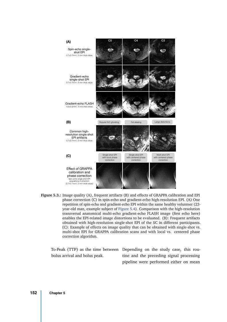
github.com/marcocastellaro/dsc-mri-toolbox

github.com/marcocastellaro/dsc-mri-toolbox

Spin-echo single-shot EPI

0.7×0.7mm2, 5-mm thick slices

Gradient-echo single-shot EPI


Gradient-echo FLASH


Common high-resolution single-shot

EPI artifacts0.7×0.7mm2, 5-mm thick slices

Effect of GRAPPA calibration and

phase correctionSpin-echo single-shot EPI acquisitions in phantom

(0.7×0.7mm2, 5-mm thick slices)

Large distortionsFat aliasingNyquist N/2 ghosting

Single-shot EPI

with centered phase

correction

Multi-shot EPI

with centered phase

correction

Single-shot EPI

with local phase

correction

(A)

(B)

(C)

C5 C4 C3

Figure 5.3.: Image quality (A), frequent artifacts (B) and effects of GRAPPA calibration and EPIphase correction (C) in spin-echo and gradient-echo high-resolution EPI. (A) Onerepetition of spin-echo and gradient-echo EPI within the same healthy volunteer (23-year-old man, example subject of Figure 5.4). Comparison with the high-resolutiontransversal anatomical multi-echo gradient-echo FLASH image (first echo here)enables the EPI-related image distortions to be evaluated. (B): Frequent artifactsobtained with high-resolution single-shot EPI of the SC in different participants.(C): Example of effects on image quality that can be obtained with single-shot vs.multi-shot EPI for GRAPPA calibration scans and with local vs. centered phasecorrection algorithm.

To-Peak (TTP) as the time between

bolus arrival and bolus peak.

Depending on the study case, this rou-

tine and the preceding signal processing

pipeline were performed either on mean

152 Chapter 5

signal in cord across the three slices, slice-

wise or voxel-wise.

Results

Single-shot EPI image quality

Figure 5.3 compares the image quality

of spin-echo and gradient-echo EPI within

a healthy volunteer. Large signal dropout

at the periphery of the SC can be observed

with gradient-echo. Based on the anatom-

ical gradient-echo FLASH image, gradient-

echo EPI showed larger image distortions

compared to spin-echo. Figure 5.3 also

shows typical artifacts of high-resolution

single-shot EPI. Nyquist N/2 ghosting ar-

tifacts could usually be addressed with a

better shimming if achievable (not trivial).

Among all datasets, 3/27 slices in total had

to be discarded because of fat aliasing ar-

tifacts. The effects of the GRAPPA calibra-

tion scan mode and phase correction algo-

rithms used can be observed in the last row

of Figure 5.3 for acquisition in phantoms.

Although it is the default option in most

product sequences, single-shot EPI GRAPPA

calibration does not seem optimal to avoid

Nyquist N/2 ghosting. A “local” phase cor-

rection, as often referenced by MRI man-

ufacturers (estimation of a k-space phase

line-dependent shift in addition to a global

term), is therefore advised.

Effect of breathing

Figure 5.4 compares the signal stability

between apnea and free breathing condi-

tions, along with the free breathing signal

after motion correction and breathing fre-

quencies filtering, both with spin-echo and

gradient-echo preparation. Signal oscilla-

tions during free breathing are clearly miti-

gated during apnea. The mean tSD in cord

(all slices) increased from 0.64 s−1 in ap-

nea to 1.22 s−1 in free breathing with spin-

echo, and from 0.75 s−1 to 1.75 s−1 with

gradient-echo. Rigid motion correction and

breathing filtering enabled a tSD of 0.65 s−1

and 0.90 s−1 to be recovered, respectively.

Breathing-induced signal fluctuations were

higher with gradient-echo, which was ex-

pected given the higher sensitivity to sus-

ceptibility variations of the T2∗-weighted

signal. No clear slice-dependent effect of

breathing stood out, either at the individual

or group (3 subjects) level (Figure 5.4, right

column).

In-vivo DSC results

Figure 5.5 presents the DSC results ob-

tained with gadolinium injection in healthy

volunteers. The contrast agent bolus was

clearly visible in every subject. As expected,

the bolus peak obtained with spin-echo

(2.0 s−1) was lower than with gradient-echo

(10.3 s−1 in average across the subjects).

However, signal stability was better with

5.2 Manuscript 153

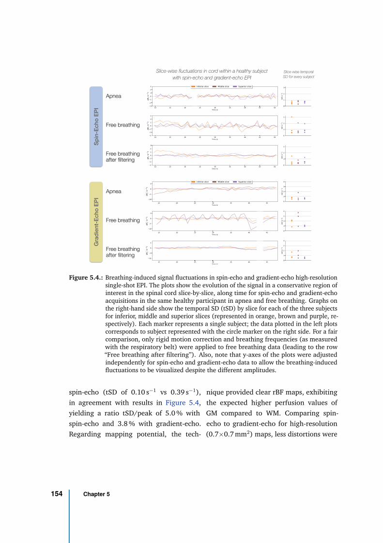
Apnea

Free breathing

Free breathing after filtering

Sp

in-E

ch

o E

PI

Apnea

Free breathing

Free breathing after filtering

Gra

die

nt-

Ech

o E

PI

Slice-wise fluctuations in cord within a healthy subject

with spin-echo and gradient-echo EPI

Slice-wise temporal

SD for every subject

Figure 5.4.: Breathing-induced signal fluctuations in spin-echo and gradient-echo high-resolutionsingle-shot EPI. The plots show the evolution of the signal in a conservative region ofinterest in the spinal cord slice-by-slice, along time for spin-echo and gradient-echoacquisitions in the same healthy participant in apnea and free breathing. Graphs onthe right-hand side show the temporal SD (tSD) by slice for each of the three subjectsfor inferior, middle and superior slices (represented in orange, brown and purple, re-spectively). Each marker represents a single subject; the data plotted in the left plotscorresponds to subject represented with the circle marker on the right side. For a faircomparison, only rigid motion correction and breathing frequencies (as measuredwith the respiratory belt) were applied to free breathing data (leading to the row“Free breathing after filtering”). Also, note that y-axes of the plots were adjustedindependently for spin-echo and gradient-echo data to allow the breathing-inducedfluctuations to be visualized despite the different amplitudes.

spin-echo (tSD of 0.10 s−1 vs 0.39 s−1),

in agreement with results in Figure 5.4,

yielding a ratio tSD/peak of 5.0 % with

spin-echo and 3.8 % with gradient-echo.

Regarding mapping potential, the tech-

nique provided clear rBF maps, exhibiting

the expected higher perfusion values of

GM compared to WM. Comparing spin-

echo to gradient-echo for high-resolution

(0.7×0.7 mm2) maps, less distortions were

154 Chapter 5

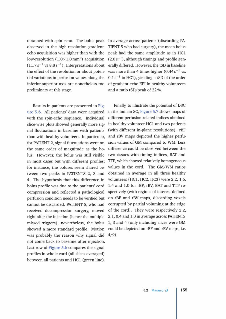
obtained with spin-echo. The bolus peak

observed in the high-resolution gradient-

echo acquisition was higher than with the

low-resolution (1.0×1.0 mm2) acquisition

(11.7 s−1 vs 8.8 s−1). Interpretations about

the effect of the resolution or about poten-

tial variations in perfusion values along the

inferior-superior axis are nonetheless too

preliminary at this stage.

Results in patients are presented in Fig-

ure 5.6. All patients’ data were acquired

with the spin-echo sequence. Individual

slice-wise plots showed generally more sig-

nal fluctuations in baseline with patients

than with healthy volunteers. In particular,

for PATIENT 2, signal fluctuations were on

the same order of magnitude as the bo-

lus. However, the bolus was still visible

in most cases but with different profiles:

for instance, the boluses seem shared be-

tween two peaks in PATIENTS 2, 3 and

4. The hypothesis that this difference in

bolus profile was due to the patients’ cord

compression and reflected a pathological

perfusion condition needs to be verified but

cannot be discarded. PATIENT 5, who had

received decompression surgery, moved

right after the injection (hence the multiple

missed triggers); nevertheless, the bolus

showed a more standard profile. Motion

was probably the reason why signal did

not come back to baseline after injection.

Last row of Figure 5.6 compares the signal

profiles in whole cord (all slices averaged)

between all patients and HC1 (green line).

In average across patients (discarding PA-

TIENT 5 who had surgery), the mean bolus

peak had the same amplitude as in HC1

(2.0 s−1), although timings and profile gen-

erally differed. However, the tSD in baseline

was more than 4 times higher (0.44 s−1 vs.

0.1 s−1 in HC1), yielding a tSD of the order

of gradient-echo EPI in healthy volunteers

and a ratio tSD/peak of 22 %.

Finally, to illustrate the potential of DSC

in the human SC, Figure 5.7 shows maps of

different perfusion-related indices obtained

in healthy volunteer HC1 and two patients

(with different in-plane resolutions). rBF

and rBV maps depicted the higher perfu-

sion values of GM compared to WM. Less

difference could be observed between the

two tissues with timing indices, BAT and

TTP, which showed relatively homogeneous

values in the cord. The GM/WM ratios

obtained in average in all three healthy

volunteers (HC1, HC2, HC3) were 2.2, 1.6,

1.4 and 1.0 for rBF, rBV, BAT and TTP re-

spectively (with regions of interest defined

on rBF and rBV maps, discarding voxels

corrupted by partial voluming at the edge

of the cord). They were respectively 2.2,

2.1, 0.4 and 1.0 in average across PATIENTS

1, 3 and 4 (only including slices were GM

could be depicted on rBF and rBV maps, i.e.

4/9).

5.2 Manuscript 155

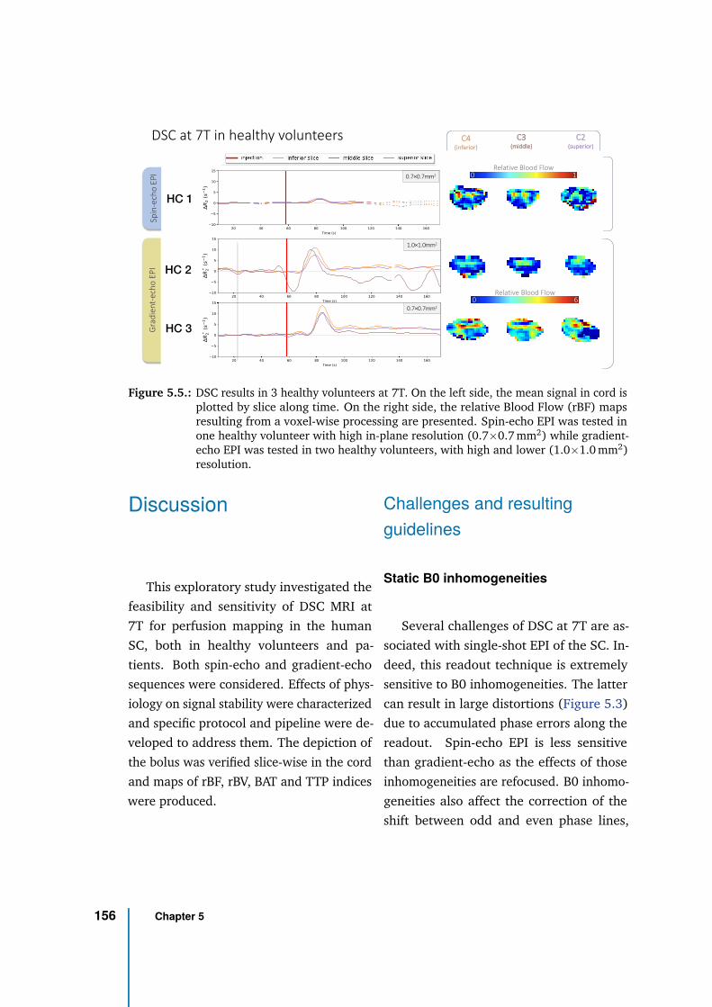
DSC at 7T in healthy volunteersS

pin

-ech

o E

PI

Gra

die

nt-

ech

o E

PI

0 6

Relative Blood Flow

0 1

Relative Blood Flow

0.7×0.7mm2

C4(inferior)

C3(middle)

C2(superior)

HC 1

HC 2

HC 3

1.0×1.0mm2

0.7×0.7mm2

Figure 5.5.: DSC results in 3 healthy volunteers at 7T. On the left side, the mean signal in cord isplotted by slice along time. On the right side, the relative Blood Flow (rBF) mapsresulting from a voxel-wise processing are presented. Spin-echo EPI was tested inone healthy volunteer with high in-plane resolution (0.7×0.7 mm2) while gradient-echo EPI was tested in two healthy volunteers, with high and lower (1.0×1.0 mm2)resolution.

Discussion

This exploratory study investigated the

feasibility and sensitivity of DSC MRI at

7T for perfusion mapping in the human

SC, both in healthy volunteers and pa-

tients. Both spin-echo and gradient-echo

sequences were considered. Effects of phys-

iology on signal stability were characterized

and specific protocol and pipeline were de-

veloped to address them. The depiction of

the bolus was verified slice-wise in the cord

and maps of rBF, rBV, BAT and TTP indices

were produced.

Challenges and resulting

guidelines

Static B0 inhomogeneities

Several challenges of DSC at 7T are as-

sociated with single-shot EPI of the SC. In-

deed, this readout technique is extremely

sensitive to B0 inhomogeneities. The latter

can result in large distortions (Figure 5.3)

due to accumulated phase errors along the

readout. Spin-echo EPI is less sensitive

than gradient-echo as the effects of those

inhomogeneities are refocused. B0 inhomo-

geneities also affect the correction of the

shift between odd and even phase lines,

156 Chapter 5

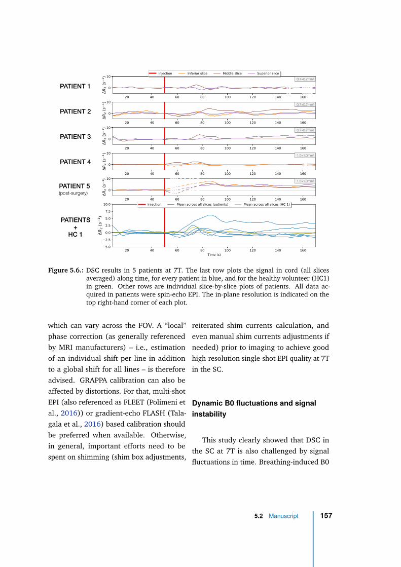
PATIENT 1

PATIENT 2

PATIENT 3

PATIENT 4

PATIENT 5

(post-surgery)

PATIENTS

+

HC 1

0.7×0.7mm2

0.7×0.7mm2

0.7×0.7mm2

1.0×1.0mm2

1.0×1.0mm2

Figure 5.6.: DSC results in 5 patients at 7T. The last row plots the signal in cord (all slicesaveraged) along time, for every patient in blue, and for the healthy volunteer (HC1)in green. Other rows are individual slice-by-slice plots of patients. All data ac-quired in patients were spin-echo EPI. The in-plane resolution is indicated on thetop right-hand corner of each plot.

which can vary across the FOV. A “local”

phase correction (as generally referenced

by MRI manufacturers) – i.e., estimation

of an individual shift per line in addition

to a global shift for all lines – is therefore

advised. GRAPPA calibration can also be

affected by distortions. For that, multi-shot

EPI (also referenced as FLEET (Polimeni et

al., 2016)) or gradient-echo FLASH (Tala-

gala et al., 2016) based calibration should

be preferred when available. Otherwise,

in general, important efforts need to be

spent on shimming (shim box adjustments,

reiterated shim currents calculation, and

even manual shim currents adjustments if

needed) prior to imaging to achieve good

high-resolution single-shot EPI quality at 7T

in the SC.

Dynamic B0 fluctuations and signal

instability

This study clearly showed that DSC in

the SC at 7T is also challenged by signal

fluctuations in time. Breathing-induced B0

5.2 Manuscript 157

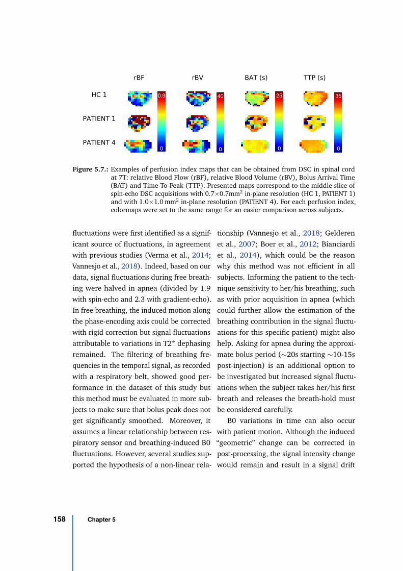
0

0.9 40 25 35

0 0 0

Figure 5.7.: Examples of perfusion index maps that can be obtained from DSC in spinal cordat 7T: relative Blood Flow (rBF), relative Blood Volume (rBV), Bolus Arrival Time(BAT) and Time-To-Peak (TTP). Presented maps correspond to the middle slice ofspin-echo DSC acquisitions with 0.7×0.7mm2 in-plane resolution (HC 1, PATIENT 1)and with 1.0×1.0 mm2 in-plane resolution (PATIENT 4). For each perfusion index,colormaps were set to the same range for an easier comparison across subjects.

fluctuations were first identified as a signif-

icant source of fluctuations, in agreement

with previous studies (Verma et al., 2014;

Vannesjo et al., 2018). Indeed, based on our

data, signal fluctuations during free breath-

ing were halved in apnea (divided by 1.9

with spin-echo and 2.3 with gradient-echo).

In free breathing, the induced motion along

the phase-encoding axis could be corrected

with rigid correction but signal fluctuations

attributable to variations in T2* dephasing

remained. The filtering of breathing fre-

quencies in the temporal signal, as recorded

with a respiratory belt, showed good per-

formance in the dataset of this study but

this method must be evaluated in more sub-

jects to make sure that bolus peak does not

get significantly smoothed. Moreover, it

assumes a linear relationship between res-

piratory sensor and breathing-induced B0

fluctuations. However, several studies sup-

ported the hypothesis of a non-linear rela-

tionship (Vannesjo et al., 2018; Gelderen

et al., 2007; Boer et al., 2012; Bianciardi

et al., 2014), which could be the reason

why this method was not efficient in all

subjects. Informing the patient to the tech-

nique sensitivity to her/his breathing, such

as with prior acquisition in apnea (which

could further allow the estimation of the

breathing contribution in the signal fluctu-

ations for this specific patient) might also

help. Asking for apnea during the approxi-

mate bolus period (∼20s starting ∼10-15s

post-injection) is an additional option to

be investigated but increased signal fluctu-

ations when the subject takes her/his first

breath and releases the breath-hold must

be considered carefully.

B0 variations in time can also occur

with patient motion. Although the induced

“geometric” change can be corrected in

post-processing, the signal intensity change

would remain and result in a signal drift

158 Chapter 5

along time. Finally, B0 fluctuations along

acquisition can cause image artifacts to be

enhanced along time. In particular, as re-

ported in MR angiography (Irwan et al.,

2007), it is common to see Nyquist N/2

ghosting mixed with GRAPPA artifacts exac-

erbated during the passage of the contrast

agent. Coming in the FOV through multiple

inlets in the neck, the contrast agent may

modify the susceptibility in multiple points,

which, depending on the shimming qual-

ity, might disturb the 7T B0 field and the

GRAPPA reconstruction algorithm.

Cardiac beat is also a source of mo-

tion for SC and its direct surrounding en-

vironment, mainly CSF. Indeed, CSF pulsa-

tions induce complex cord motion along the

inferior-superior axis and in the transver-

sal plane (Figley et al., 2007; Figley et al.,

2008). This source of bias is expected to be

addressed with cardiac gating targeting the

quiescent window for acquisition. Neverthe-

less, CSF pulsations and resulting flow pat-

terns might not be perfectly regular across

cardiac cycles, which is likely to add dy-

namic B0 variations in the vicinity of the

cord and increase the signal instability.

Potentials and perspectives of

DSC MRI at 7T in the human

spinal cord

The DSC technique was able to provide

high-resolution maps of relative perfusion

indices with a clear distinction between GM

and WM perfusion (in agreement with exist-

ing literature (Turnbull, 1973; Tator et al.,

1997; Duhamel et al., 2008; Duhamel et

al., 2009)) in every individual slice within

healthy volunteers and in slightly less than

one third of the slices within patients. To

the best of the authors’ knowledge, such re-

sults have never been achieved so far. They

suggest a promising potential of DSC for re-

liable assessment of perfusion abnormalities

in the SC, with an identification of affected

pathways, and open the door to new clinical

investigations on the involvement of perfu-

sion in SC pathologies. Establishment of

earlier biomarker of tissue degeneration are

also a significant potential of the technique.

Regarding the comparison between spin-

echo and gradient-echo preparations, even

though gradient-echo has not been tested

in patients yet and are needed, some com-

parison elements can already be stated.

First, thanks to the refocusing pulse of spin-

echo, image distortions and signal dropout

with susceptibility effects are mitigated com-

pared to gradient-echo. However, this re-

focusing pulse also comes with more en-

ergy deposition and SAR was an important

limitation for the number of slices and the

use of the optimal flip angles at 7T. Sec-

ondly, although it is too preliminary to draw

conclusion on the ratio tSD/bolus peak for

each preparation in healthy subjects, signal

fluctuations in patients with spin-echo were

increased by more than 4 as compared to

healthy controls, compromising the sensitiv-

ity to bolus. These increased signal fluctua-

5.2 Manuscript 159

tions in patients are thought to be related to

(1) more irregular breathing patterns (see

breathing period SD in Figure 5.3), (2) a de-

creased coil sensitivity (B1- field) associated

with generally longer distances between

coil and SC (elderly subjects with gener-

ally larger morphology) and (3) a lower

signal because of higher SAR restrictions

making impossible to reach the optimal flip

angle in the cord. Point (1) is likely to bias

the estimation of breathing frequencies and

consequently, compromise the efficacy of

the filtering. Points (2) and (3) resulted in

a lower signal and thus, an increased contri-

bution of the physiological noise in the sig-

nal. The effect of deglutition on signal sta-

bility should also be investigated. Patients

are often associated with more discomfort

during acquisition than healthy volunteers.

It is therefore important to dedicate more

time to installation and information about

SC MRI challenges. Those signal fluctua-

tions would probably have been larger with

gradient-echo, as suggested by results in

Figure 5.4, but bolus peak is expected to

be higher, hence the importance of future

investigations to assess the performance of

gradient-echo in patients.

The technical challenges related to ultra-

high field MRI are likely to be addressed

in the coming years. Parallel transmission

is a promising avenue to address SAR re-

strictions and B1+ inhomogeneities. Design

for SC coil arrays could be optimized to im-

prove transmit and receive fields efficiency

in a wider range of morphologies. A de-

sign with both anterior and posterior ele-

ments have already been proposed for cervi-

cal cord imaging at 7T (Zhang et al., 2017).

Dynamic slice-wise shimming or real-time

shimming such as SC coil arrays integrating

real-time correction of breathing-induced

B0 fluctuations (Topfer et al., 2018) would

further help to reduce distortions and signal

instability. Finally, multiband acquisitions

(Feinberg et al., 2013) with adequate coil

design could be used to increase the number

of slices and cover the whole cervical cord

despite cardiac gating, but at the expense

of SAR and SNR (Preibisch et al., 2015).

Conclusion

DSC at 7T showed great potential for

perfusion mapping in the human SC within

a clinical context, despite multiple chal-

lenges. In healthy volunteers, individual

slice-wise maps of rBF and rBV were ob-

tained, discriminating the GM perfusion

from the WM, which, to the best of our

knowledge, have never obtained so far.

However, signal stability needs to be im-

proved in acquisition conditions associated

with patients. More investigations, es-

pecially using gradient-echo preparation,

distortions, larger inferior-superior cover-

age and SAR management are needed but

guidelines to ensure successful results could

be identified and were here proposed.

160 Chapter 5

Acknowledgements

The authors would like to thank Sylviane

Confort-Gouny, Véronique Gimenez, Lauri-

ane Pini, Claire Costes, Patrick Viout, Muriel

Juge-Boulogne and Virginie Véla for study

logistics.

This project received funding from

the European Union’s Horizon 2020 re-

search and innovation program under the

Marie Skłodowska-Curie grant agreement

#713750. Also, it was carried out with fi-

nancial support from the Regional Council

of Provence-Alpes-Cote d’Azur and with fi-

nancial support from the A*MIDEX (#ANR-

11-IDEX-0001-02), funded by the Investisse-

ments d’Avenir project funded by the French

Government, managed by the French Na-

tional Research Agency (ANR).

This work was performed within a lab-

oratory member of France Life Imaging

network (#ANR-11-INBS-0006), supported

by the following funding sources: 7T-

AMI-ANR-11-EQPX-0001, A*MIDEX-EI-13-

07-130115-08.38-7T-AMISTART and CNRS

(Centre National de la Recherche Scien-

tifique).

References

Alsop, David C., John A. Detre, Xavier Go-

lay, et al. (Jan. 2015). “Recommended

implementation of arterial spin-labeled

perfusion MRI for clinical applications:

A consensus of the ISMRM perfusion

study group and the European consor-

tium for ASL in dementia: Recommended

Implementation of ASL for Clinical Ap-

plications”. en. In: Magnetic Resonance

in Medicine 73.1, pp. 102–116. DOI: 10.

1002/mrm.25197 (cit. on p. 145).

Andersson, Jesper L. R., Stefan Skare, and

John Ashburner (Oct. 2003). “How to cor-

rect susceptibility distortions in spin-echo

echo-planar images: application to dif-

fusion tensor imaging”. In: NeuroImage

20.2, pp. 870–888. DOI: 10.1016/S1053-

8119(03)00336-7 (cit. on p. 150).

Aracki-Trenkic, Aleksandra, Bruno Law-ye,

Zoran Radovanovic, et al. (July 2020).

“ASL perfusion in acute ischemic stroke:

The value of CBF in outcome prediction”.

en. In: Clinical Neurology and Neuro-

surgery 194, p. 105908. DOI: 10.1016/j.

clineuro.2020.105908 (cit. on p. 145).

Avants, Brian B., Nicholas J. Tustison, Gang

Song, et al. (2011). “A reproducible eval-

uation of ANTs similarity metric per-

formance in brain image registration”.

In: NeuroImage 54, pp. 2033–2044. DOI:

http : / / dx . doi . org / 10 . 1016 /

j . neuroimage . 2010 . 09 . 025 (cit. on

p. 150).

Beattie, Michael S., Akhlaq A. Farooqui, and

Jacqueline C. Bresnahan (Oct. 2000). “Re-

view of Current Evidence for Apoptosis

After Spinal Cord Injury”. en. In: Jour-

nal of Neurotrauma 17.10, pp. 915–925.

DOI: 10.1089/neu.2000.17.915 (cit. on

p. 145).

5.2 Manuscript 161

https://doi.org/10.1002/mrm.25197


https://doi.org/10.1016/S1053-8119(03)00336-7

https://doi.org/10.1016/S1053-8119(03)00336-7

https://doi.org/10.1016/j.clineuro.2020.105908

https://doi.org/10.1016/j.clineuro.2020.105908

https://doi.org/http://dx.doi.org/10.1016/j.neuroimage.2010.09.025

https://doi.org/http://dx.doi.org/10.1016/j.neuroimage.2010.09.025

https://doi.org/10.1089/neu.2000.17.915

Bianciardi, Marta, Jonathan R. Polimeni,

Kawin Setsompop, et al. (2014). “Evalua-

tion of dynamic off-resonance correction

of respiratory instability in MRI signals

for high-order spherical harmonic basis

set and multivariate modeling of respi-

ratory sources”. In: Proc. Int. Soc. Magn.

Reson. Med. 22. Milan, Italy, p. 1623 (cit.

on p. 158).

Boer, Vincent O., Bart L. vd Bank, Gerard

van Vliet, Peter R. Luijten, and Dennis

W. J. Klomp (Feb. 2012). “Direct B0 field

monitoring and real-time B0 field updat-

ing in the human breast at 7 tesla”. en.

In: Magnetic Resonance in Medicine 67.2,

pp. 586–591. DOI: 10.1002/mrm.23272

(cit. on p. 158).

Donahue, Manus J., Jun Hua, James J.

Pekar, and Peter C.M. van Zijl (Feb.

2009). “Effect of inflow of fresh blood

on vascular-space-occupancy (VASO) con-

trast”. en. In: Magnetic Resonance in

Medicine 61.2, pp. 473–480. DOI: 10 .

1002/mrm.21804 (cit. on p. 146).

Duhamel, Guillaume, Virginie Callot,

Patrick J. Cozzone, and Frank Kober

(2008). “Spinal cord blood flow measure-

ment by arterial spin labeling”. In: Mag-

netic Resonance in Medicine 59, pp. 846–

854. DOI: 10.1002/mrm.21567 (cit. on

pp. 145, 146, 159).

Duhamel, Guillaume, Virginie Callot,

Patrick Decherchi, et al. (2009). “Mouse

lumbar and cervical spinal cord blood

flow measurements by arterial spin la-

beling: Sensitivity optimization and first

application”. In: Magnetic Resonance in

Medicine 62, pp. 430–439. DOI: 10.1002/

mrm.22015 (cit. on p. 159).

Ellingson, Benjamin M., Davis C. Wood-

worth, Kevin Leu, Noriko Salamon, and

Langston T. Holly (Aug. 2019). “Spinal

Cord Perfusion MR Imaging Implicates

Both Ischemia and Hypoxia in the Patho-

genesis of Cervical Spondylosis”. en. In:

World Neurosurgery 128, e773–e781. DOI:

10.1016/j.wneu.2019.04.253 (cit. on

p. 146).

Fehlings, M. G. and G. Skaf (Dec. 1998). “A

review of the pathophysiology of cervi-

cal spondylotic myelopathy with insights

for potential novel mechanisms drawn

from traumatic spinal cord injury”. eng.

In: Spine 23.24, pp. 2730–2737 (cit. on

p. 146).

Feinberg, David A. and Kawin Setsompop

(Apr. 2013). “Ultra-fast MRI of the hu-

man brain with simultaneous multi-slice

imaging”. en. In: Journal of Magnetic Res-

onance 229, pp. 90–100. DOI: 10.1016/j.

jmr.2013.02.002 (cit. on p. 160).

Figley, C.R. and P.W. Stroman (July 2007).

“Investigation of human cervical and up-

per thoracic spinal cord motion: Implica-

tions for imaging spinal cord structure

and function”. en. In: Magnetic Resonance

in Medicine 58.1, pp. 185–189. DOI: 10.

1002/mrm.21260 (cit. on p. 159).

Figley, C.R., D. Yau, and P.W. Stroman (Sept.

2008). “Attenuation of Lower-Thoracic,

Lumbar, and Sacral Spinal Cord Motion:

Implications for Imaging Human Spinal

162 Chapter 5







https://doi.org/10.1016/j.wneu.2019.04.253

https://doi.org/10.1016/j.jmr.2013.02.002




Cord Structure and Function”. en. In:

American Journal of Neuroradiology 29.8,

pp. 1450–1454. DOI: 10 . 3174 / ajnr .

A1154 (cit. on p. 159).

Gelderen, P. van, J.A. de Zwart, P. Starewicz,

R.S. Hinks, and J.H. Duyn (Feb. 2007).

“Real-time shimming to compensate for

respiration-induced B0 fluctuations”. en.


pp. 362–368. DOI: 10.1002/mrm.21136

(cit. on p. 158).

Gilmor, MICHELLE L, ST Rouse, CRAIG J

Heilman, NR Nash, and AI Levey (1998).

“Receptor fusion proteins and analysis”.

In: Receptor localization. Ed. by MA Ari-

ano. Vol. 19. Publisher: WILEY. New York,

pp. 75–90 (cit. on p. 145).

Girard, Olivier M., Virginie Callot, Ben-

jamin Robert, Patrick J. Cozzone, and

Guillaume Duhamel (2013). “Perfusion

MRI of the Human Cervical Spinal Cord

using Arterial Spin Labeling”. In: Proceed-

ings of the 21st annual meeting of the In-

ternational Society for Magnetic Resonance

in Medicine. Salt Lake City, Utah, USA,

p. 0349 (cit. on p. 146).

Irwan, Roy, Daniël D. Lubbers, Pieter A. van

der Vleuten, et al. (June 2007). “Parallel

imaging for first-pass myocardial perfu-

sion”. en. In: Magnetic Resonance Imaging

25.5, pp. 678–683. DOI: 10.1016/j.mri.

2006.10.012 (cit. on p. 159).

Kalsi-Ryan, Sukhvinder, Spyridon K. Karadi-

mas, and Michael G. Fehlings (Nov. 2012).

“Cervical Spondylotic Myelopathy: The

Clinical Phenomenon and the Current

Pathobiology of an Increasingly Preva-

lent and Devastating Disorder”. In: The

Neuroscientist 19.4. Publisher: SAGE Pub-

lications Inc STM, pp. 409–421. DOI:

10 . 1177 / 1073858412467377 (cit. on

p. 145).

Kellner, Elias, Bibek Dhital, Valerij G. Kiselev,

and Marco Reisert (Nov. 2016). “Gibbs-

ringing artifact removal based on local

subvoxel-shifts”. en. In: Magnetic Reso-

nance in Medicine 76.5, pp. 1574–1581.

DOI: 10 . 1002 / mrm . 26054 (cit. on

p. 150).

Kraff, Oliver and Harald H. Quick (Dec.

2017). “7T: Physics, safety, and potential

clinical applications: 7T: Physics, Safety,

Applications”. en. In: Journal of Mag-

netic Resonance Imaging 46.6, pp. 1573–

1589. DOI: 10.1002/jmri.25723 (cit. on

p. 146).

Le Bihan, D, E Breton, D Lallemand, et al.

(Aug. 1988). “Separation of diffusion and

perfusion in intravoxel incoherent motion

MR imaging.” en. In: Radiology 168.2,

pp. 497–505. DOI: 10.1148/radiology.

168.2.3393671 (cit. on p. 145).

Lu, Hanzhang, Meng Law, Yulin Ge, et al.

(Apr. 2008). “Quantitative measurement

of spinal cord blood volume in humans

using vascular-space-occupancy MRI”. en.

In: NMR in Biomedicine 21.3, pp. 226–

232. DOI: 10.1002/nbm.1185 (cit. on

p. 146).

Lévy, Simon, Stanislas Rapacchi, Aurélien

Massire, et al. (Feb. 2020). “Intravoxel

Incoherent Motion at 7 Tesla to quan-

5.2 Manuscript 163

https://doi.org/10.3174/ajnr.A1154



https://doi.org/10.1016/j.mri.2006.10.012


https://doi.org/10.1177/1073858412467377


https://doi.org/10.1002/jmri.25723

https://doi.org/10.1148/radiology.168.2.3393671


https://doi.org/10.1002/nbm.1185

tify human spinal cord perfusion: Limi-

tations and promises”. en. In: Magnetic

Resonance in Medicine, mrm.28195. DOI:

10.1002/mrm.28195 (cit. on p. 146).

Maggioni, M., V. Katkovnik, K. Egiazar-

ian, and A. Foi (Jan. 2013). “Nonlocal

Transform-Domain Filter for Volumetric

Data Denoising and Reconstruction”. en.

In: IEEE Transactions on Image Processing

22.1, pp. 119–133. DOI: 10.1109/TIP.

2012.2210725 (cit. on p. 150).

Massire, Aurélien, Manuel Taso, Pierre

Besson, et al. (Dec. 2016). “High-

resolution multi-parametric quantitative

magnetic resonance imaging of the hu-

man cervical spinal cord at 7T”. In: Neu-

roImage 143, pp. 58–69. DOI: 10.1016/


pp. 147, 150).

Nair, G. and X. P. Hu (2010). “Perfusion

Imaging of the Human Cervical Spinal

Cord”. In: Proceedings of the 19th annual

meeting of the International Society for

Magnetic Resonance in Medicine. Stock-

holm, Sweden, p. 4083 (cit. on p. 146).

Noebauer-Huhmann, I M, O Kraff, V Juras,

et al. (2008). “MR Contrast Media at

7Tesla - Preliminary Study on Relaxivi-

ties”. en. In: Proceedings of the 16th an-

nual meeting of the International Soci-

ety for Magnetic Resonance in Medicine.

Toronto, Canada, p. 1457 (cit. on p. 146).

Parkes Laura M., Rashid Waqar, Chard De-

clan T., and Tofts Paul S. (Mar. 2004).

“Normal cerebral perfusion measure-

ments using arterial spin labeling: Repro-

ducibility, stability, and age and gender ef-

fects”. In: Magnetic Resonance in Medicine

51.4, pp. 736–743. DOI: 10.1002/mrm.

20023 (cit. on p. 146).

Polimeni, Jonathan R., Himanshu Bhat,

Thomas Witzel, et al. (Feb. 2016). “Re-

ducing sensitivity losses due to respira-

tion and motion in accelerated echo pla-

nar imaging by reordering the autocali-

bration data acquisition: Reducing Losses

in Accelerated EPI with FLEET-ACS”. en.


pp. 665–679. DOI: 10.1002/mrm.25628

(cit. on p. 157).

Polimeni, Jonathan R. and Kâmil Uludag

(Mar. 2018). “Neuroimaging with ultra-

high field MRI: Present and future”. In:

Neuroimaging with Ultra-high Field MRI:

Present and Future 168, pp. 1–6. DOI: 10.

1016/j.neuroimage.2018.01.072 (cit.

on p. 146).

Preibisch, Christine, J. Gabriel Castrillón G.,

Martin Bührer, and Valentin Riedl (Sept.

2015). “Evaluation of Multiband EPI Ac-

quisitions for Resting State fMRI”. en.

In: PLOS ONE 10.9. Ed. by Wang Zhan,

e0136961. DOI: 10.1371/journal.pone.

0136961 (cit. on p. 160).

Rohrer, Martin, Hans Bauer, Jan

Mintorovitch, Martin Requardt, and

Hanns-Joachim Weinmann (Nov. 2005).

“Comparison of Magnetic Properties of

MRI Contrast Media Solutions at Differ-

ent Magnetic Field Strengths:” en. In:

Investigative Radiology 40.11, pp. 715–

164 Chapter 5


https://doi.org/10.1109/TIP.2012.2210725

https://doi.org/10.1109/TIP.2012.2210725

https://doi.org/10.1016/j.neuroimage.2016.08.055







https://doi.org/10.1371/journal.pone.0136961


724. DOI: 10.1097/01.rli.0000184756.

66360.d3 (cit. on p. 146).

Schubert, Martin (2017). “Natural Course

of Disease of Spinal Cord Injury”. In: Neu-

rological Aspects of Spinal Cord Injury. Ed.

by Norbert Weidner, Rüdiger Rupp, and

Keith E. Tansey. Cham: Springer Interna-

tional Publishing, pp. 77–105. DOI: 10.

1007/978- 3- 319- 46293- 6_4 (cit. on

p. 145).

Scouten, A. and R.T. Constable (Feb. 2008).

“VASO-based calculations of CBV change:

Accounting for the dynamic CSF volume”.

en. In: Magnetic Resonance in Medicine

59.2, pp. 308–315. DOI: 10.1002/mrm.

21427 (cit. on p. 146).

Staff News Brief (Oct. 2017). “Siemens ob-

tains first CE approval for ultra-high-field

7T MR scanner”. In: Appl Radiol (cit. on

p. 146).

Talagala, S. Lalith, Joelle E. Sarlls, Siyuan

Liu, and Souheil J. Inati (June 2016). “Im-

provement of temporal signal-to-noise ra-

tio of GRAPPA accelerated echo planar

imaging using a FLASH based calibration

scan: Temporal SNR of GRAPPA Accel-

erated EPI”. en. In: Magnetic Resonance

in Medicine 75.6, pp. 2362–2371. DOI:

10.1002/mrm.25846 (cit. on p. 157).

Tator, Charles H. and Izumi Koyanagi

(1997). “Vascular mechanisms in the

pathophysiology of human spinal cord in-

jury”. English. In: Journal of Neurosurgery

86.3. Publisher: Journal of Neurosurgery

Publishing Group, pp. 483–492. DOI: 10.

3171 / jns . 1997 . 86 . 3 . 0483 (cit. on

pp. 145, 159).

Topfer, Ryan, Alexandru Foias, Nikola

Stikov, and Julien Cohen-Adad (Sept.

2018). “Real-time correction of

respiration-induced distortions in the

human spinal cord using a 24-channel

shim array: Real-Time B 0 Shimming in

the Spinal Cord”. en. In: Magnetic Reso-

nance in Medicine 80.3, pp. 935–946. DOI:

10.1002/mrm.27089 (cit. on p. 160).

Turnbull, Ian M. (Jan. 1973). “Blood Sup-

ply of the Spinal Cord: Normal and

Pathological Considerations”. In: Neuro-

surgery 20.CN_suppl_1, pp. 56–84. DOI:

10.1093/neurosurgery/20.CN_suppl_

1.56 (cit. on pp. 145, 159).

Vannesjo, S. Johanna, Karla L. Miller, Stuart

Clare, and Irene Tracey (Feb. 2018). “Spa-

tiotemporal characterization of breathing-

induced B0 field fluctuations in the cer-

vical spinal cord at 7T”. en. In: NeuroIm-

age 167, pp. 191–202. DOI: 10 . 1016 /


pp. 146, 158).

Verma, Tanya and Julien Cohen-Adad (Dec.

2014). “Effect of respiration on the B0

field in the human spinal cord at 3T: Ef-

fect of Respiration on B0 Field in Human

Spinal Cord”. en. In: Magnetic Resonance


10 . 1002 / mrm . 25075 (cit. on pp. 146,

158).

Zhang, Bei, Alan C. Seifert, Joo-won Kim,

Joseph Borrello, and Junqian Xu (Oct.

2017). “7 Tesla 22-channel wrap-around

5.2 Manuscript 165

https://doi.org/10.1097/01.rli.0000184756.66360.d3


https://doi.org/10.1007/978-3-319-46293-6_4

https://doi.org/10.1007/978-3-319-46293-6_4




https://doi.org/10.3171/jns.1997.86.3.0483

https://doi.org/10.3171/jns.1997.86.3.0483


https://doi.org/10.1093/neurosurgery/20.CN_suppl_1.56

https://doi.org/10.1093/neurosurgery/20.CN_suppl_1.56




coil array for cervical spinal cord and

brainstem imaging: 7T Cervical Spinal

Cord Coil”. en. In: Magnetic Resonance


10.1002/mrm.26538 (cit. on p. 160).

166 Chapter 5



The DSC technique at 7T clearly exhibited a higher potential than IVIM for human

spinal cord perfusion mapping in addition to its short acquisition time. In healthy

volunteers, individual slice-wise maps of relative BF and BV, discriminating the gray

matter perfusion from the white matter could be obtained. To the best of my knowledge,

such maps have never published up to now. However, the robustness of the technique

was challenged for acquisitions in pathological conditions. Higher SAR restrictions

limiting the flip angle might have resulted in a lower signal and higher contribution of

the physiological noise. In addition, more irregular breathing might have lessened the

efficiency of the breathing filtering, resulting in larger signal instabilities than within

healthy volunteers. Nevertheless, those investigative data are extremely precious given

the increased difficulty to recruit subjects for research and developments involving a

contrast agent injection, which comes with additional logistics and constraints for the

patient, as well as impossible multiple trials for the acquisition operator. Yet, the relative

BF and BV maps obtained are promising. Limitations specific to 7T should soon be solved.

The SAR restrictions and limited number of slices are likely to be overcome with parallel

transmission. Multi-band acquisitions with adequate coil design could also allow more

slices and cover the whole cervical cord. Finally, breathing-induced field fluctuations

might additionally be mitigated by upcoming real-time shimming technologies.

5.3 Concluding remarks 167

Biomechanical comparison of

spinal cord compression types

occurring in Degenerative

Cervical Myelopathy

6

6.1 Foreword

This chapter is devoted to biomechanical modeling of typical spinal cord compressions

as found in Degenerative Cervical Myelopathy (DCM) patients, making the third article

of the thesis, accepted for publication in the journal Clinical Biomechanics on September

3, 2020.

In this publication, the goal was first to characterize the DCM compressions in order to

design the most representative biomechanical simulations. Quantitative indices for DCM

compressions reported in literature were collected and compared to the Spine Model

for Safety and Surgery (SM2S) dimensions. In addition, those indices were measured

within a cohort of 20 DCM patients. Based on those data, a compression of 30 % in

spinal cord Cross-Sectional Area (CSA) was selected as critical threshold for myelopathy.

Furthermore, patient’s anatomical MRI enabled four main types of compression to be

identified. Those four types were simulated using the SM2S to the same compression

threshold of 30 % compared to initial CSA. An exhaustive quantification of the normal,

shear and Von Mises stresses along different axes (time, inferior-superior axis, spinal

cord sub-regions) allowed the different compression types to be compared. An anterior

compression applied on the entire antero-posterior diameter of the cord appeared as the

most injurious.

This work was the subject of an invited talk at the 2020 SIMBIO-M Conference, which

was awarded the best presentation prize.

169

6.2 Manuscript

Title:

Biomechanical comparison of spinal cord compressiontypes occurring in Degenerative Cervical Myelopathy

Authors:

Simon Lévya,b,c,d, Guillaume Baucherd,e, Pierre-Hugues Roched,e, Morgane Evinc,d, Vir-

ginie Callota,b,d, Pierre-Jean Arnouxc,d

Affiliations:a Aix-Marseille Univ, CNRS, CRMBM, Marseille, Franceb APHM, Hopital Universitaire Timone, CEMEREM, Marseille, Francec Aix-Marseille Univ, IFSTTAR, LBA, Marseille, Franced iLab-Spine International Associated Laboratory, Marseille-Montreal, France-Canadae APHM, Hopital Nord, Neurosurgery Department, Marseille, France

Journal:

Submitted on March 21, 2020 to Clinical Biomechanics, recommended for minor revisions

on July 21, 2020

Abstract

Background: Degenerative Cervical

Myelopathy (DCM) results from spine de-

generations narrowing the spinal canal and

inducing cord compressions. Prognosis is

challenging. This study aimed at simulating

typical spinal cord compressions observed

in DCM patients with a realistic model to

better understand pathogenesis for later

prediction of patients’ evolution.

Methods: A 30% reduction in cord cross-

sectional area at C5-C6 was defined as

myelopathy threshold based on DCM fea-

tures from literature and MRI measure-

ments in 20 patients. Four main compres-

sion types were extracted from MRIs and

simulated with a comprehensive 3D finite el-

ement spine model. Median diffuse, median

focal and lateral types were modeled as disk

herniation while circumferential type addi-

tionally involved ligamentum flavum hyper-

trophy. All stresses were quantified along

inferior-superior axis, compression develop-

ment and across atlas-defined spinal cord

regions.

170 Chapter 6

Findings: Anterior gray and white matter

globally received the highest stress while

lateral pathways were the least affected.

Median diffuse compression induced the

highest stresses. Circumferential type fo-

cused stresses in posterior gray matter.

Along inferior-superior axis, those two types

showed a peak of constraints at compres-

sion site while median focal and lateral

types showed lower values but extending

further.

Interpretation: Median diffuse type would

be the most detrimental based on stress

amplitude. Anterior regions would be

the most at risk, except for circumferen-

tial type where posterior regions would be

equally affected. In addition to applying

constraints, ischemia could be a significant

component explaining the early demyelina-

tion reported in lateral pathways. Moving

towards patient-specific simulations, biome-

chanical models could become strong pre-

dictors for degenerative changes.

Keywords: spinal cord, spinal cord com-

pression, degenerative cervical myelopathy,

finite element modelling, herniated disk, lig-

amentum flavum hypertrophy

Introduction

Degenerative Cervical Myelopathy

(DCM) is the most common progressive

non-traumatic disorder of the spinal cord

(SC) in elderly population with a prevalence

of 605 per million people in North America

(Nouri et al., 2015). Eighty-seven percent

of global population above 60 years old is

estimated to present one or more severely

degenerated cervical levels(Matsumoto et

al., 1998). DCM results from degenerative

changes of the cervical spine with aging

causing spinal canal stenosis, cord compres-

sion and eventually myelopathy. Degenera-

tive changes are multiple and can happen

concurrently or individually (Nouri et al.,

2015). On the anterior side of the cord,

intervertebral disk (IVD) draining induc-

ing disk material migration into the spinal

canal, spondylitis with osteophytes devel-

opment and hypertrophy of the posterior

longitudinal ligament (PLL) progressively

narrow spinal canal. On the opposite side,

spinal canal is reduced by hypertrophy of

the ligamentum flavum. Compression is sus-

pected to first disrupt tissue perfusion and

metabolism, which then leads to expanding

tissue necrosis (cell loss, axonal demyeli-

nation, Wallerian degeneration)(Ellingson

et al., 2019; Fehlings et al., 1998; Ahuja

et al., 2017). In addition to the chronic

static cord compression, everyday life neck

motion (flexion, extension) is expected to

add repeated traumas to the cord (dynamic

effects). However, the respective roles of

those processes in tissue degeneration yield-

ing myelopathy remain unknown. The

multiple processes aforementioned result in

a high variability of the patients’ clinical pre-

sentation and of the compression patterns

6.2 Manuscript 171

observed on MRI or CT scans. Severity of

symptoms is therefore hardly predictable.

The SC compression process is intrinsi-

cally mechanical. Finite element models

are therefore very well suited to study SC

compression processes occurring in DCM de-

generation. Several biomechanical studies

already proposed DCM compression mod-

els. Nishida et al. (2012) first studied the

contribution of static and dynamic anterior

compressions of the cord for three differ-

ent patterns (central, lateral, diffuse). Kim

et al. (2013) investigated the individual ef-

fects of different patterns of ossification of

the PLL and ligamentum flavum. Nishida et

al. (2015) then explored the static and dy-

namic effects of the ossification of the PLL.

Finally, Khuyagbaatar et al. (2015) modeled

both single-level and multi-level compres-

sions caused by ossification of the PLL.

In all those studies, the different pro-

cesses involved were not simulated concur-

rently. Resulting stresses were only ana-

lyzed based on visual assessment of the

stress maps or by quantification at a spe-

cific compression stage and level without

comparison across spinal pathways, com-

pression development or inferior-superior

(I-S) axis. Moreover, models were often sim-

plified with unnatural compression loading,

which is useful to identify the specific ef-

fects of a given process but could miss some

important features induced by the natural

human anatomy.

In this work, simulations of the main

compression patterns derived from clinical

MR exploration of 20 DCM patients were

designed using a detailed and comprehen-

sive cervical SC model. Quantitative com-

pression feature measurements from MRI

data and derived from literature were inte-

grated. All resulting constraints were ana-

lyzed along the I-S axis, along compression

development and across atlas-defined SC re-

gions to identify the specificity of each com-

pression pattern. Such analysis aimed at

providing insights to better understand the

multiple degenerative processes associated

with DCM and identify the most detrimental

pattern. Those simulations could guide clin-

icians in the treatment, surgical planning

and/or prognosis of this pathology.

Methods

Compression features from

literature review

Most frequently affected level IVD level

C5-C6 is the most frequently compressed

level in DCM patients (Northover et al.,

2012; Edwards et al., 1983). It is hypoth-

esized to be due to the higher mobility of

that segment compared to others (Penning,

1978). It is also among the two segments

with smallest anteroposterior (A-P) spinal

canal diameter (Ogino et al., 1983).

172 Chapter 6

Compression threshold inducing tissue de-

generation Morphologic indices proposed

in literature to evaluate DCM compressions

were collected in Table 6.1: spinal canal

A-P diameter (Edwards et al., 1983; Ogino

et al., 1983; Arnold, 1955; Adams et al.,

1971; Burrows, 1963), SC Cross-Sectional

Area (CSA)(Penning et al., 1986; Li et

al., 2018), A-P compression ratio (Li et

al., 2018) (see Figure 6.1 for definitions).

DCM index value was normalized by control

value when available.

Compression features from

acquired MRI data

To complete and balance the literature

data heterogeneity, anatomical MR images

of 20 diagnosed DCM adult patients were

examined. Local ethics committee approval

(Comité de Protection des Personnes Sud-

Marseille I, Marseille, France/ID RCB: 2011-

A00929-32) and written consent of partici-

pants were obtained prior acquisitions.

Most frequently affected level C4-C5 and

C5-C6 were the most frequent compression

levels (N=8 respectively) in the cohort.

Compression threshold inducing tissue de-

generation The morphological features of

DCM compressions were inspected on T2*

-weighted and T1-weighted images. The

following measurements were performed

on T1-weighted images at the maximum

compression level (Figure 6.1): A-P and R-L

spinal canal diameters, A-P and R-L cord

diameters, spinal canal and cord CSA, cord

A-P occupation, cord CSA occupation. Mea-

surements were performed manually using

Horos (horosproject.org).

Compression features for simulations

Considering indices based on SC more di-

rectly related to the constraint applying

on it, and given the consistency between

values derived from MRI data and literature

(see Table 6.1 and Results section), the SC

CSA was elected to define the compression

threshold. A SC CSA of 70% with respect to

the initial CSA (equivalent to a 30% CSA re-

duction) was defined as threshold inducing

myelopathy at C5-C6 IVD level.

Observed compression types Anatomical

MRI images showed various compression

patterns which were classified into 4 main

types (Figure 6.2) in agreement with previ-

ous studies (Nishida et al., 2012; Fujiwara

et al., 1986; Nishida et al., 2014): median

diffuse (N=9), median focal (N=2), lateral

(N=5), circumferential (N=4).

Simulations

Finite element model description The

Spine Model for Safety and Surgery (El-

Rich et al., 2009; Wagnac et al., 2012) was

6.2 Manuscript 173

horosproject.org

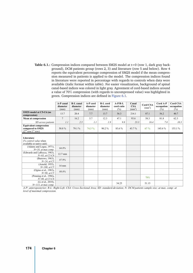
Table 6.1.: Compression indices compared between SM2S model at t=0 (row 1, dark gray back-ground), DCM patients group (rows 2, 3) and literature (row 5 and below). Row 4reports the equivalent percentage compression of SM2S model if the mean compres-sion measured in patients is applied to the model. The compression indices foundin literature were reported in percentage with regards to controls when data wereavailable (italic format within table). For easier visualization, background of spinalcanal-based indices was colored in light gray. Agreement of cord-based indices arounda value of 70% compression (with regards to uncompressed value) was highlighted ingreen. Compression indices are defined in Figure 6.1.

A-P canal

diameter

(mm)

R-L canal

diameter

(mm)

A-P cord

diameter

(mm)

R-L cord

diameter

(mm)

A-P/R-L

cord ratio

(%)

Canal

CSA

(mm2)

Cord CSA

(mm2)

Cord A-P

occupation

(%)

Cord CSA

occupation

(%)

SM2S model at C5-C6 (no

compression) 13.7 20.4 7.7 13.7 56.3 214.1 87.1 56.2 40.7

Mean at compression 7 16.2 5.7 12.3 47.1 93.6 58.3 81.8 62.3

SD across patients 1.1 2.5 1.1 1.9 9.8 23.3 16.4 7.8 10.3

Equivalent compression

compared to SM2S

(2nd row/1st row) 50.8 % 79.1 % 74.3 % 90.2 % 83.6 % 43.7 % 67 % 145.6 % 153.1 %

Literature

(% control value when available or native unit)

(Adams and Logue, 1971),

N=18, at max comp. 64.8%

(Edwards and LaRocca, 1983), N=63, at C5-C6

12.7 mm

(Burrows, 1963),

N=24, at C5 87.9%

(Arnold, 1955), N=100, at C5

14 mm

(Ogino et al., 1983),

N=90, at C5 88.8%

(Penning et al., 1986),

N=80, at C5-C6 70%

(Li et al., 2018),

N=113, at max comp. 34.25 51.15

A-P: anteroposterior; R-L: Right-Left; CSA: Cross-Sectional Area; SD: standard-deviation; N: DCM patients sample size; at max. comp: at

level of maximal compression.

174 Chapter 6

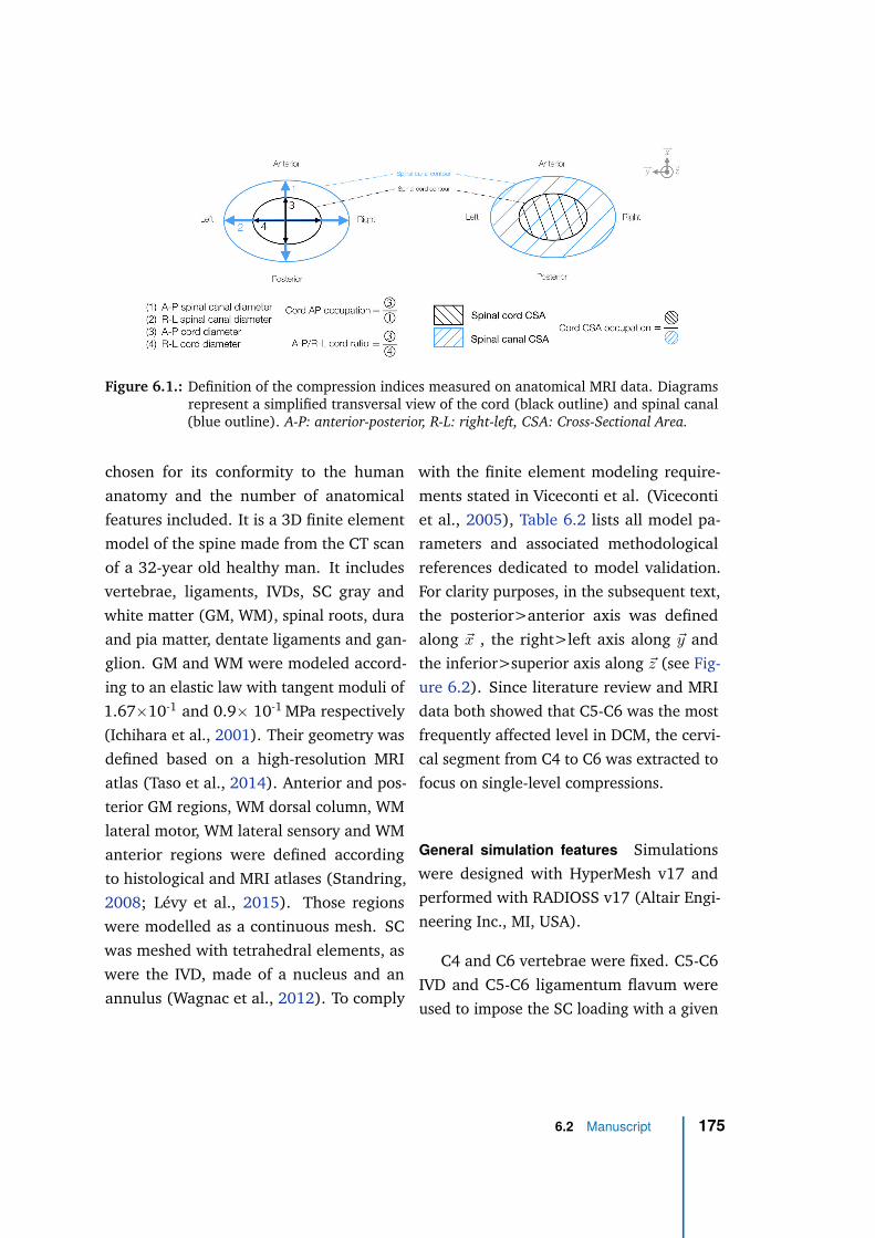
Figure 6.1.: Definition of the compression indices measured on anatomical MRI data. Diagramsrepresent a simplified transversal view of the cord (black outline) and spinal canal(blue outline). A-P: anterior-posterior, R-L: right-left, CSA: Cross-Sectional Area.

chosen for its conformity to the human

anatomy and the number of anatomical

features included. It is a 3D finite element

model of the spine made from the CT scan

of a 32-year old healthy man. It includes

vertebrae, ligaments, IVDs, SC gray and

white matter (GM, WM), spinal roots, dura

and pia matter, dentate ligaments and gan-

glion. GM and WM were modeled accord-

ing to an elastic law with tangent moduli of

1.67×10-1 and 0.9× 10-1 MPa respectively

(Ichihara et al., 2001). Their geometry was

defined based on a high-resolution MRI

atlas (Taso et al., 2014). Anterior and pos-

terior GM regions, WM dorsal column, WM

lateral motor, WM lateral sensory and WM

anterior regions were defined according

to histological and MRI atlases (Standring,

2008; Lévy et al., 2015). Those regions

were modelled as a continuous mesh. SC

was meshed with tetrahedral elements, as

were the IVD, made of a nucleus and an

annulus (Wagnac et al., 2012). To comply

with the finite element modeling require-

ments stated in Viceconti et al. (Viceconti

et al., 2005), Table 6.2 lists all model pa-

rameters and associated methodological

references dedicated to model validation.

For clarity purposes, in the subsequent text,

the posterior>anterior axis was defined

along ~x , the right>left axis along ~y and

the inferior>superior axis along ~z (see Fig-

ure 6.2). Since literature review and MRI

data both showed that C5-C6 was the most

frequently affected level in DCM, the cervi-

cal segment from C4 to C6 was extracted to

focus on single-level compressions.

General simulation features Simulations

were designed with HyperMesh v17 and

performed with RADIOSS v17 (Altair Engi-

neering Inc., MI, USA).

C4 and C6 vertebrae were fixed. C5-C6

IVD and C5-C6 ligamentum flavum were

used to impose the SC loading with a given

6.2 Manuscript 175

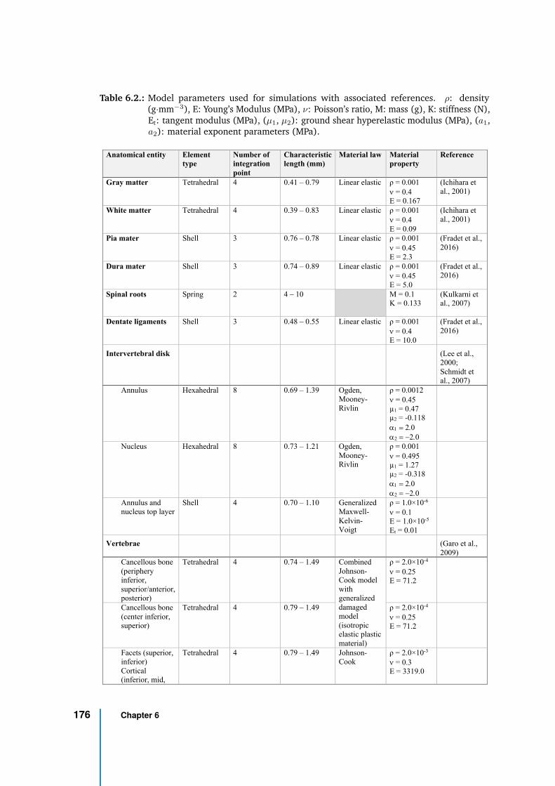
Table 6.2.: Model parameters used for simulations with associated references. ρ: density(g·mm−3), E: Young’s Modulus (MPa), ν: Poisson’s ratio, M: mass (g), K: stiffness (N),Et: tangent modulus (MPa), (µ1, µ2): ground shear hyperelastic modulus (MPa), (a1,a2): material exponent parameters (MPa).

Anatomical entity Element

type

Number of

integration

point

Characteristic

length (mm)

Material law Material

property

Reference

Gray matter Tetrahedral 4 0.41 – 0.79 Linear elastic ρ = 0.001

n = 0.4

E = 0.167

(Ichihara et

al., 2001)

White matter Tetrahedral 4 0.39 – 0.83 Linear elastic ρ = 0.001

n = 0.4

E = 0.09

(Ichihara et

al., 2001)

Pia mater Shell 3 0.76 – 0.78 Linear elastic ρ = 0.001

n = 0.45

E = 2.3

(Fradet et al.,

2016)

Dura mater Shell 3 0.74 – 0.89 Linear elastic ρ = 0.001

n = 0.45

E = 5.0

(Fradet et al.,

2016)

Spinal roots Spring

2 4 – 10 M = 0.1

K = 0.133

(Kulkarni et

al., 2007)

Dentate ligaments Shell 3 0.48 – 0.55 Linear elastic ρ = 0.001

n = 0.4

E = 10.0

(Fradet et al.,

2016)

Intervertebral disk (Lee et al.,

2000;

Schmidt et

al., 2007)

Annulus Hexahedral 8 0.69 – 1.39 Ogden,

Mooney-

Rivlin

ρ = 0.0012

n = 0.45

µ1 = 0.47

µ2 = -0.118

a1 = 2.0

a2 = -2.0

Nucleus Hexahedral 8 0.73 – 1.21 Ogden,

Mooney-

Rivlin

ρ = 0.001

n = 0.495

µ1 = 1.27

µ2 = -0.318

a1 = 2.0

a2 = -2.0

Annulus and

nucleus top layer

Shell 4 0.70 – 1.10 Generalized

Maxwell-

Kelvin-

Voigt

ρ = 1.0×10-6

n = 0.1

E = 1.0×10-5

Et = 0.01

Vertebrae (Garo et al.,

2009)

Cancellous bone

(periphery

inferior,

superior/anterior,

posterior)

Tetrahedral 4 0.74 – 1.49 Combined

Johnson-

Cook model

with

generalized

damaged

model

(isotropic

elastic plastic

material)

ρ = 2.0×10-4

n = 0.25

E = 71.2

Cancellous bone

(center inferior,

superior)

Tetrahedral 4 0.79 – 1.49 ρ = 2.0×10-4

n = 0.25

E = 71.2

Facets (superior,

inferior)

Cortical

(inferior, mid,

Tetrahedral 4 0.79 – 1.49 Johnson-

Cook

ρ = 2.0×10-3

n = 0.3

E = 3319.0

176 Chapter 6

superior/anterior,

posterior)

Endplate center

(inferior,

superior)

Shell 3 0.91 – 1.00 Johnson-

Cook

ρ = 2.0×10-4

n = 0.3

E = 71.2

Endplate

periphery

(inferior,

superior)

Shell 3 0.94 – 0.99 Johnson-

Cook

ρ = 2.0×10-3

n = 0.3

E = 3319.0

Posterior

element

Tetrahedral 4 0.79 – 1.55 Combined

Johnson-

Cook model

with

generalized

damaged

model

(isotropic

elastic plastic

material)

ρ = 2.0×10-3

n = 0.3

E = 3319.0

Posterior

element layer

Shell 3 0.95-0.96 Johnson-

Cook

ρ = 2.0×10-3

n = 0.3

E = 3319.0

Ligaments (Beauséjour

et al., 2019)

Anterior

Longitudinal

Ligament

Shell 4 0.40 – 0.58 Tabulated

elastic plastic

piecewise

linear

ρ = 0.01

Posterior

Longitudinal

Ligament


elastic plastic

piecewise

linear

ρ = 0.01

Nuchal

Ligament


elastic plastic

piecewise

linear

ρ = 0.01

Ligamentum

flavum


elastic plastic

piecewise

linear

ρ = 0.01

Joint Capsule Shell 3 0.89 – 0.99 Tabulated

elastic plastic

piecewise

linear

ρ = 0.01

Interspinous

Ligament


elastic plastic

piecewise

linear

ρ = 0.01

ρ: density (g.mm-3), E: Young’s Modulus (MPa), n: Poisson’s ratio, M: mass (g), K: stiffness (N), E : tangent modulus

6.2 Manuscript 177

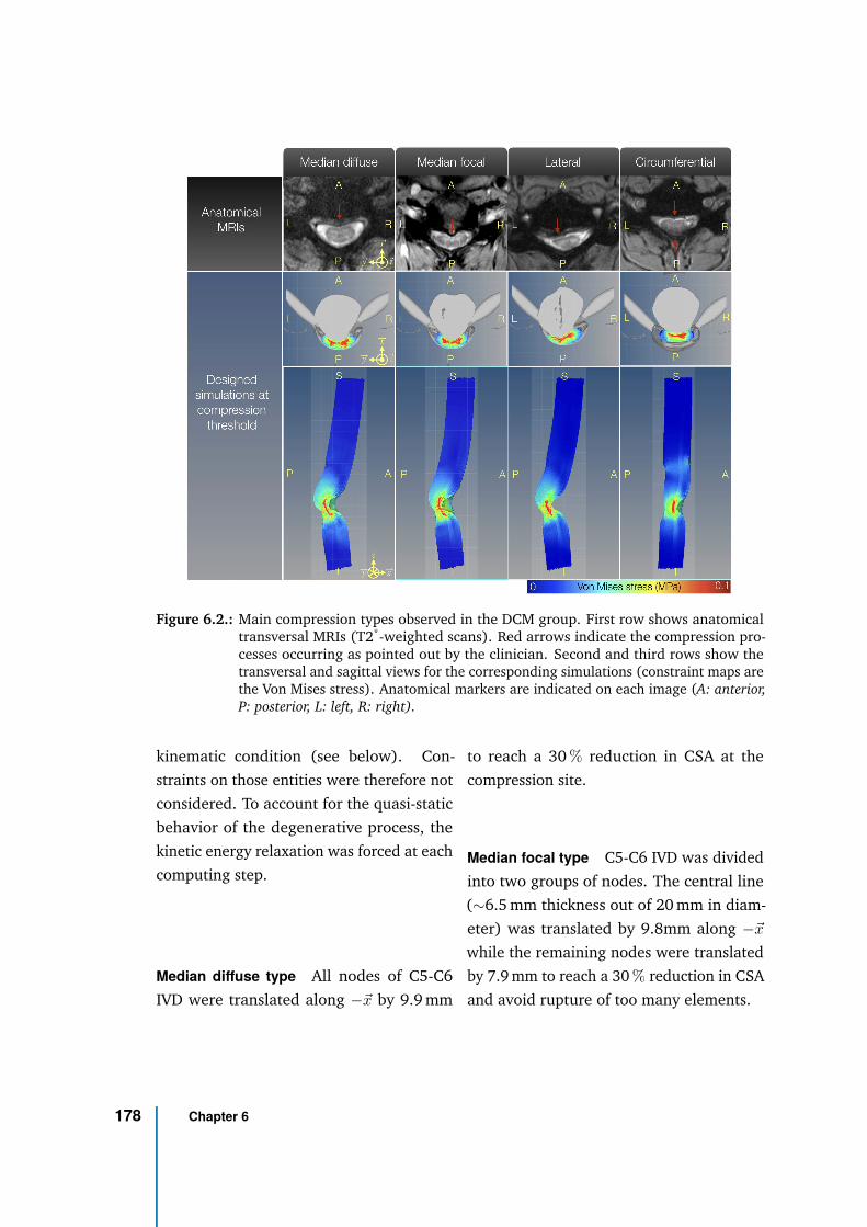
Figure 6.2.: Main compression types observed in the DCM group. First row shows anatomicaltransversal MRIs (T2*-weighted scans). Red arrows indicate the compression pro-cesses occurring as pointed out by the clinician. Second and third rows show thetransversal and sagittal views for the corresponding simulations (constraint maps arethe Von Mises stress). Anatomical markers are indicated on each image (A: anterior,P: posterior, L: left, R: right).

kinematic condition (see below). Con-

straints on those entities were therefore not

considered. To account for the quasi-static

behavior of the degenerative process, the

kinetic energy relaxation was forced at each

computing step.

Median diffuse type All nodes of C5-C6

IVD were translated along −~x by 9.9 mm

to reach a 30 % reduction in CSA at the

compression site.

Median focal type C5-C6 IVD was divided

into two groups of nodes. The central line

(∼6.5 mm thickness out of 20 mm in diam-

eter) was translated by 9.8mm along −~x

while the remaining nodes were translated

by 7.9 mm to reach a 30 % reduction in CSA

and avoid rupture of too many elements.

178 Chapter 6

Lateral type C5-C6 IVD was divided into

four groups of nodes. The most left part of

the disk (7.4 mm thick), a central-left line

(2.5 mm thick), the central line (1.9 mm

thick) and the remaining right part of the

disk (7.6 mm thick) were translated along

−~x by 11.2 mm, 10.5 mm, 8.5 mm and

8.1 mm respectively. This design helped to

create asymmetry in the compression while

reaching a 30 % reduction in CSA.

Circumferential type All nodes of C5-

C6 IVD were translated along −~x by

4.4 mm while all nodes of C5-C6 ligamen-

tum flavum were translated along +~x by

4.4 mm.

Quantification

Stresses along X, Y, Z, shear stresses in

XY, YZ, ZX and Von Mises stress were ex-

tracted with HyperView v2017 and Com-

pose v2019.2 (Altair Engineering Inc., MI,

USA). Data were processed with Python

v3.6.

Analysis along inferior-superior axis To

mitigate outliers effect, the 95th percentile

of each constraint absolute value within SC

was extracted at each millimeter for each

compression type and plotted along the I-S

axis. The absolute value made this metric in-

dependent from the direction of constraints.

Analysis along compression development

For each simulation step, the 95th percentile

of each constraint absolute value within SC

was extracted for each compression type.

Analysis across spinal cord regions The

95th percentile of each constraint absolute

value within each of the 6 SC regions (an-

terior and posterior GM, WM dorsal col-

umn, WM lateral motor, WM lateral sensory,

WM anterior pathways) was extracted for

each compression type and pictured on a

transversal unwrapped SC map. Note that

left and right regions were quantified to-

gether to get rid of bias caused by potential

asymmetry in compression types (e.g., lat-

eral type).

Results

Table 6.1 compares compression indices

derived from patients’ MRI data to litera-

ture. Those measurements were normal-

ized to initial SM2S model dimensions (1st

row) to determine the equivalent compres-

sion in the model. Compression indices

based on spinal canal dimensions showed

poor agreement between patients’ average

value, SM2S model and available literature

data. However, cord-based indices, and

in particular, A-P cord diameter and cord

CSA showed a rough agreement around a

30 % compression value between the mea-

surements performed on the DCM cohort

with respect to initial SM2S dimensions

6.2 Manuscript 179

and literature data with respect to controls

(equivalent to an index value of 70 % with

respect to uncompressed state).

Figure 6.2 shows the similarity obtained

between the designed simulations and

observed DCM compression patterns on

transversal MRIs. The median diffuse com-

pression is mainly caused by the migration

of a large portion of the disk into the canal

in addition to osteophyte development. In

the median focal type, the compression is

more local, predominantly caused by os-

teophyte developments and/or herniated

disk; this was modelled by a more promi-

nent migration of the central R-L line of

the disk. The lateral compression is caused

by an asymmetric degeneration of the disk

and/or osteophyte development; it was

simulated by a more prominent migration

of the left side of the disk. Finally, the

circumferential type involves an additional

process: hypertrophy and bulking of the

ligament flavum induce a posterior stenosis

of the spinal canal while disk migration

and/or osteophyte development constrict

the cord anteriorly.

A sole observation of constraint maps

(as in Figure 6.2 ) does not enable to detect

differences between compression types. For

all types, GM appears as the structure with

the most constraints, which is attributable

to its highest rigidity compared to WM.

Profiles along I-S axis look similar and so

far, history of the compression development

process is missing.

The quantitative constraints profile

along I-S axis in whole SC is presented

in Figure 6.3. Two profiles can be iden-

tified. Median diffuse and circumferential

types show a peak of the constraints at the

level of compression whereas median fo-

cal and lateral types show low stress values

but extending over a larger height of the

SC, spreading from upper C5 level down to

lower C6. Such features would not have

been detectable with a sole qualitative ob-

servation of constraint maps (Figure 6.2),

hence the value of the quantitative analysis.

Median diffuse appears as the type inducing

the highest constraint to the SC tissue with

a peak of the Von Mises stress at 0.15 MPa

and σX (stress along ~x) at 0.14 MPa. For all

types, the highest directional stress is σX

while the highest shear stress is in the ZX

plane (τZX).

Figure 6.4 presents the evolution of

constraints within cord along the develop-

ment of the pathology until compression

threshold is reached. A linear rise of the

constraints can be observed with the devel-

opment of the compression but at different

pace according to compression types. Con-

straints in SC start to increase earlier for

median focal and lateral types but at a

slower pace than other types. Median dif-

fuse shows the latest rise of the constraints

and fastest pace. Nevertheless, care must

180 Chapter 6

be taken when comparing those results as

time scale and respective individual timings

of degenerative changes are unknown and

may highly vary across population. Again,

for all types, the constraints are dominated

by σX and τZX .

Figure 6.5 presents constraints analysis

by SC sub-regions. Spinal pathways were af-

fected differently according to compression

type. Globally, highest constraint values

were found for Von Mises and directional

stresses. τXY and τY Z showed the lowest

values.

The median diffuse type showed the highest

stress values. Interestingly, this compres-

sion type also showed the highest shear

stress value (τZX in GM posterior horns).

This type also showed the highest σZ (in

anterior WM).

The median focal type also showed low-

est stress values but a similar distribution

across regions, except in GM posterior horns

apparently less affected.

The lateral type showed a very similar pro-

file as the median focal type but with lower

stress values (σX , Von Mises). Of note,

although the compression pattern is asym-

metric, the lateral pathways were not the

most affected.

Finally, the circumferential type almost

showed no shear stress and constraints were

mainly found in σX (and consequently in

Von Mises stress). Interestingly, σX was

similarly distributed between anterior and

posterior regions. This compression type

was the type showing the highest σX in pos-

terior GM horns and dorsal columns.

6.2 Manuscript 181

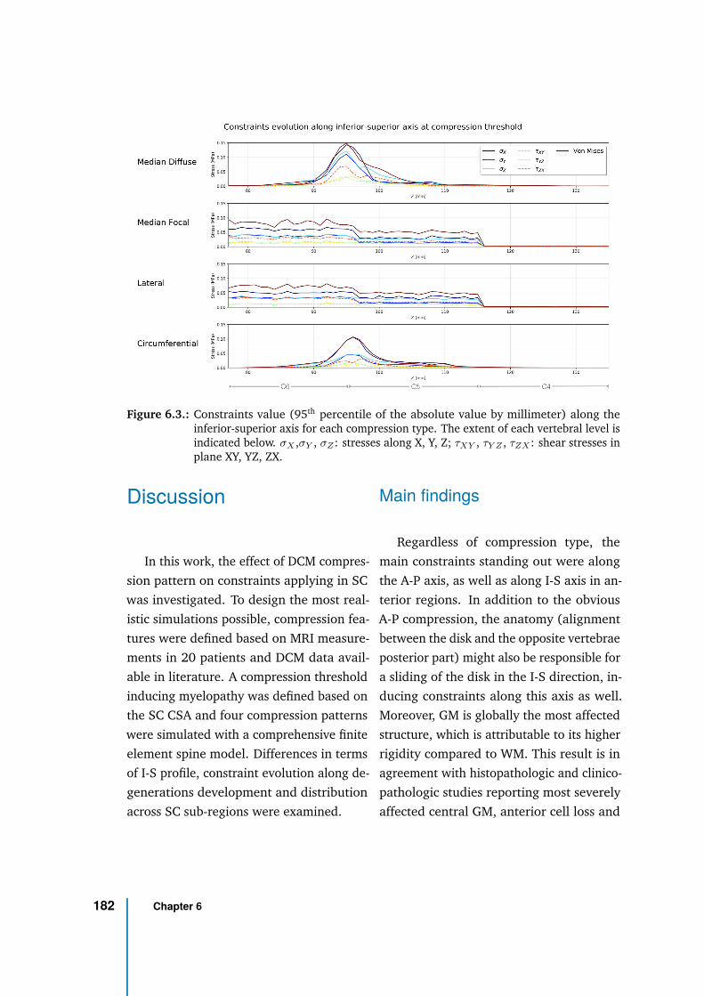
Figure 6.3.: Constraints value (95th percentile of the absolute value by millimeter) along theinferior-superior axis for each compression type. The extent of each vertebral level isindicated below. σX ,σY , σZ : stresses along X, Y, Z; τXY , τY Z , τZX : shear stresses inplane XY, YZ, ZX.

Discussion

In this work, the effect of DCM compres-

sion pattern on constraints applying in SC

was investigated. To design the most real-

istic simulations possible, compression fea-

tures were defined based on MRI measure-

ments in 20 patients and DCM data avail-

able in literature. A compression threshold

inducing myelopathy was defined based on

the SC CSA and four compression patterns

were simulated with a comprehensive finite

element spine model. Differences in terms

of I-S profile, constraint evolution along de-

generations development and distribution

across SC sub-regions were examined.

Main findings

Regardless of compression type, the

main constraints standing out were along

the A-P axis, as well as along I-S axis in an-

terior regions. In addition to the obvious

A-P compression, the anatomy (alignment

between the disk and the opposite vertebrae

posterior part) might also be responsible for

a sliding of the disk in the I-S direction, in-

ducing constraints along this axis as well.

Moreover, GM is globally the most affected

structure, which is attributable to its higher

rigidity compared to WM. This result is in

agreement with histopathologic and clinico-

pathologic studies reporting most severely

affected central GM, anterior cell loss and

182 Chapter 6

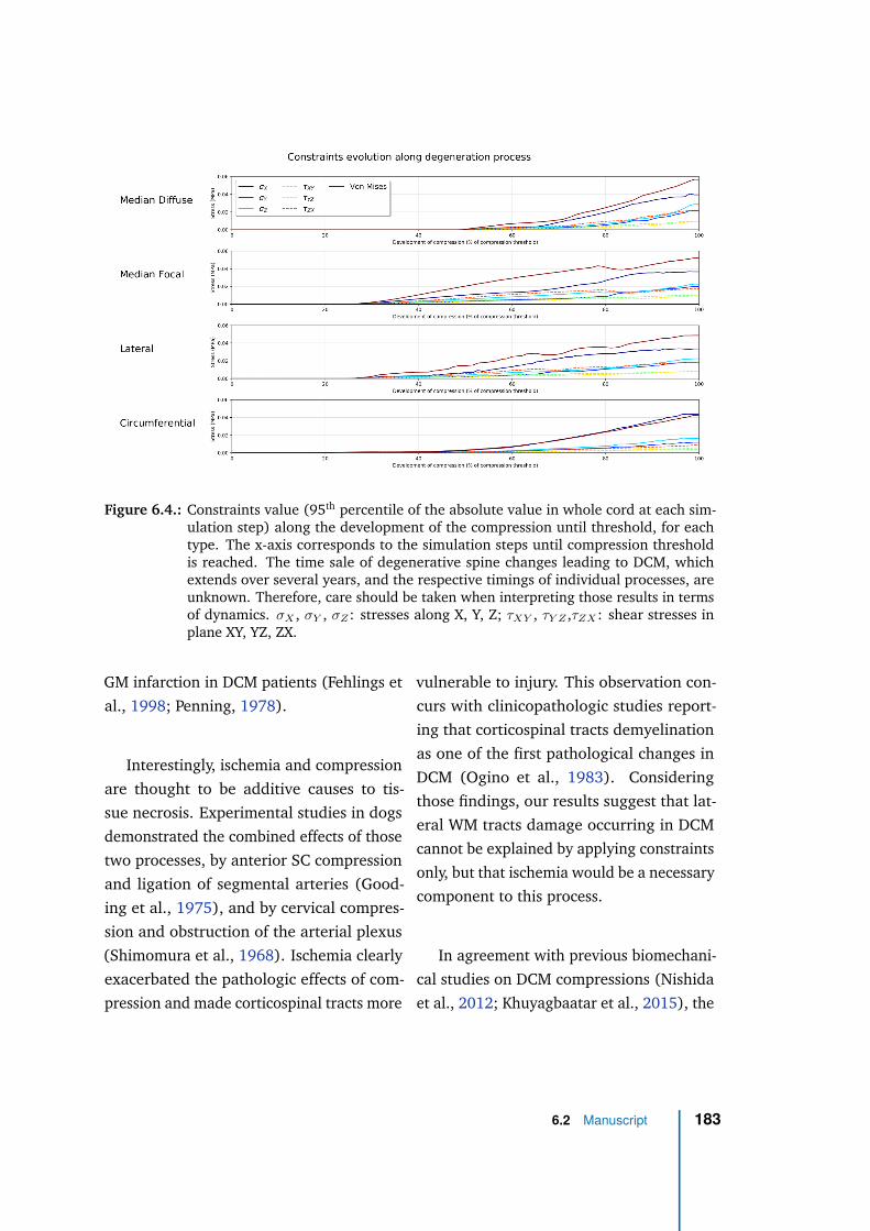
Figure 6.4.: Constraints value (95th percentile of the absolute value in whole cord at each sim-ulation step) along the development of the compression until threshold, for eachtype. The x-axis corresponds to the simulation steps until compression thresholdis reached. The time sale of degenerative spine changes leading to DCM, whichextends over several years, and the respective timings of individual processes, areunknown. Therefore, care should be taken when interpreting those results in termsof dynamics. σX , σY , σZ : stresses along X, Y, Z; τXY , τY Z ,τZX : shear stresses inplane XY, YZ, ZX.

GM infarction in DCM patients (Fehlings et

al., 1998; Penning, 1978).

Interestingly, ischemia and compression

are thought to be additive causes to tis-

sue necrosis. Experimental studies in dogs

demonstrated the combined effects of those

two processes, by anterior SC compression

and ligation of segmental arteries (Good-

ing et al., 1975), and by cervical compres-

sion and obstruction of the arterial plexus

(Shimomura et al., 1968). Ischemia clearly

exacerbated the pathologic effects of com-

pression and made corticospinal tracts more

vulnerable to injury. This observation con-

curs with clinicopathologic studies report-

ing that corticospinal tracts demyelination

as one of the first pathological changes in

DCM (Ogino et al., 1983). Considering

those findings, our results suggest that lat-

eral WM tracts damage occurring in DCM

cannot be explained by applying constraints

only, but that ischemia would be a necessary

component to this process.

In agreement with previous biomechani-

cal studies on DCM compressions (Nishida

et al., 2012; Khuyagbaatar et al., 2015), the

6.2 Manuscript 183

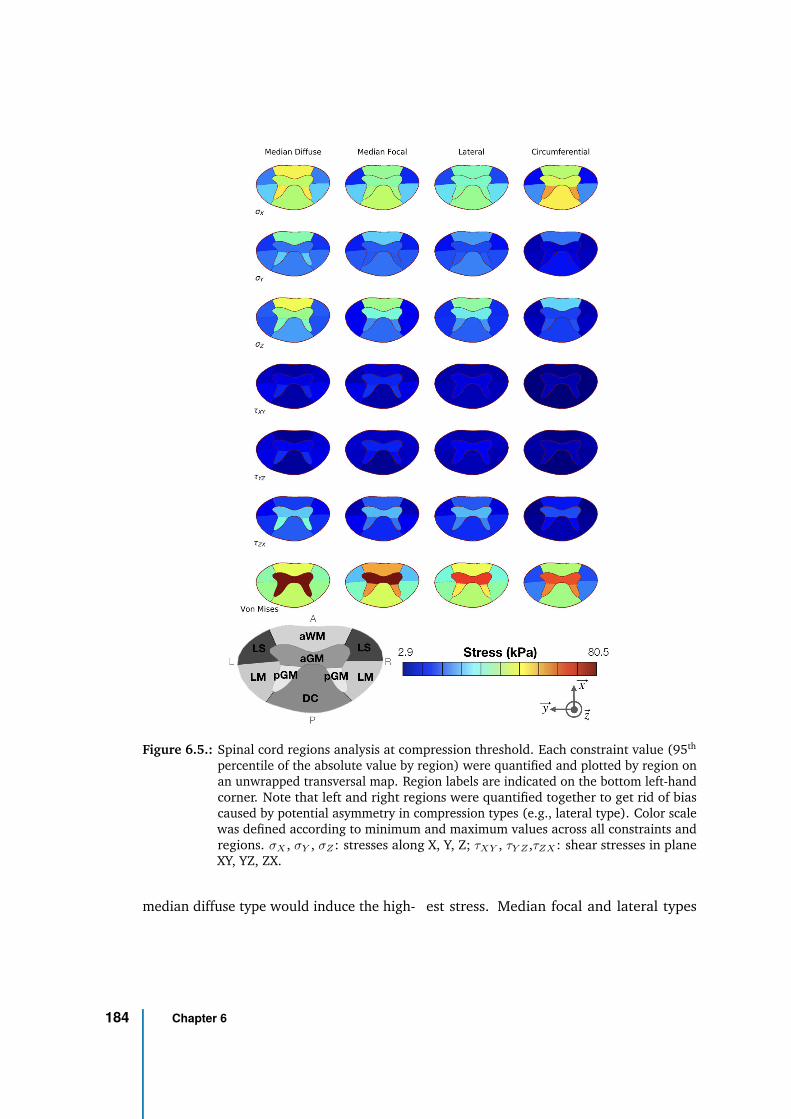
Figure 6.5.: Spinal cord regions analysis at compression threshold. Each constraint value (95th

percentile of the absolute value by region) were quantified and plotted by region onan unwrapped transversal map. Region labels are indicated on the bottom left-handcorner. Note that left and right regions were quantified together to get rid of biascaused by potential asymmetry in compression types (e.g., lateral type). Color scalewas defined according to minimum and maximum values across all constraints andregions. σX , σY , σZ : stresses along X, Y, Z; τXY , τY Z ,τZX : shear stresses in planeXY, YZ, ZX.

median diffuse type would induce the highest stress. Median focal and lateral types

184 Chapter 6

differed especially regarding the constraints

profile along the I-S axis, suggesting that

SC would need to be screened more care-

fully rostral and caudal to the compression

site for those compression patterns. This

result can be mechanically explained by the

more local compression; the cord needs to

be confined in a more restricted area, in-

volving opposite forces above and below

the compression site to clench the cord. The

circumferential type, involving both ante-

rior and posterior compression (hypertro-

phy of the ligamentum flavum) exhibited a

particular constraint distribution across SC

sub-regions. Very low shear stresses were

observed and constraints were mainly fo-

cused in the A-P axis. Effects of ligaments

ossification on the stress distribution in SC

have been studied at thoracic and cervical

levels (Kim et al., 2013; Nishida et al., 2015;

Khuyagbaatar et al., 2015) but they were

never compared to other compression types.

The current study enables to directly iden-

tify the specific effects of each type, and in

particular, the circumferential type would

be the one inducing the highest stress along

A-P axis in posterior GM horns.

Furthermore, this work investigated the

evolution of stresses in SC as DCM degener-

ations develop. Such analysis could guide

neurosurgeons in defining the critical time

to prescribe surgery. For instance, results ob-

tained here would suggest that lateral and

median focal types take more degenerative

changes (displacement) or more time to set

up and reach the threshold defined as induc-

ing myelopathy. However, to translate those

results to real life, timings of each degen-

erative process with respect to each other

need to be known. In addition, those degen-

erative processes and their timing are very

likely to vary across patients. Simulation

design specifically adapted to the patient

morphology (patient-specific simulations)

would therefore be required to predict the

pathology evolution.

Beyond that, this study proposes an ex-

haustive quantitative analysis of the con-

straints at different scales (across degen-

eration process, along I-S axis, across SC

regions) which, to the best of our knowl-

edge, has been rarely done in the literature,

probably because of the large memory size

and lack of tools available for such study.

However, such analysis is crucial to explore

and understand the tissue degeneration pro-

cesses of this pathology.

Limitations and perspectives

Compressions occurring in DCM patients

are highly variable, as are the symptoms.

For the study purpose, compression patterns

were classified into four main types. In-

terestingly, this classification was found to

be consistent across the literature (Nishida

et al., 2012; Khuyagbaatar et al., 2015).

However, real cases often mix those types

either at different intervertebral levels or

even at a single level. Designing such com-

6.2 Manuscript 185

pression patterns would be equivalent to

patient-specific simulations.

The same compression threshold was de-

fined for each type. However, given the

variability in constraints distribution, this

threshold is likely to differ across types. No

data available in literature could provide an

answer to this question. Further investiga-

tions, in association with MRI examinations

and patient-specific simulations, will look

at the definition of this threshold based on

the actual constraints value applying in the

tissue, which might be a more direct surro-

gate than the CSA. Anyhow, indices based

on spinal canal dimensions appeared less

reliable to define the myelopathy or symp-

tomatic threshold than indices based on SC

because of a larger variability.

In the current study, only static effects

of compression were considered. Dynamic

effects (with repeated neck flexion and ex-

tension) are suspected to have a significant

impact on myelopathy development too. In

a simplified model of the cervical spine, dif-

ferent effects on stress distribution across

compression types were observed (Nishida

et al., 2012) but this effect was not quanti-

fied. Inclusion of such effects in the current

model would be relevant.

Results suggest that GM tissue stiffness

for GM with regards to WM has a strong

impact on the resulting stress distribution.

Even though limited literature exists on this

topic for human, three studies (two groups)

agreed on a higher stiffness of GM com-

pared to WM, in bovine cervical cord by

tensile testing (Ichihara et al., 2001; Ichi-

hara et al., 2003) and in mice SC using

atomic force microscopic indentation and

tensile measurements (Koser et al., 2015).

One study found no significant difference

using pipette aspiration method in rabbit SC

(Ozawa et al., 2001). In this study, bovine

cervical cord values were used (stiffer GM)

(Ichihara et al., 2001). Although it is likely

to observe the same behavior in humans,

everything still needs to be shown. If the

reversed relation turned out to be shown in

humans, results of these simulations might

be challenged. Sensitivity analysis on the

impact of those parameters would provide

an estimation of the effect.

Furthermore, Koser et al. (2015) re-

ported significant difference depending on

tissue orientations, both for GM and WM.

They even found significant differences

across GM regions, with the dorsal horn

being stiffer than ventral horn, while WM

would be transversely isotropic. Obtaining

similar data for human SC would refine re-

gional analysis.

According to the acknowledged hypothe-

sis, tissue compression and ischemia would

be the main components in DCM patho-

genesis, with the two processes working

both sequentially (compression inducing

arterial obstruction causing ischemia) and

additively (ischemia exacerbating compres-

sion pathological effects) (Fehlings et al.,

186 Chapter 6

1998). For this reason, the study focused

on mechanical stresses only and strain was

discarded. Including strain in the analysis

could bring more insights in the understand-

ing of the pathology, but it would require a

more complex and accurate modeling than

the elastic law used here, with failure crite-

ria. Unfortunately, such data are not avail-

able yet.

Impacts on and of tissue perfusion were

not modeled in this study either. SC vascu-

lar network is very complex and may vary

across individuals. Moreover, characteriza-

tion of its effect on tissue mechanical prop-

erties in-vivo is highly challenging. How-

ever, as described earlier with regards to

corticospinal tracts early demyelination, is-

chemia is a key component in the patho-

genesis of DCM. A simple model of ante-

rior spinal artery and five branches was pro-

posed but only compression effects on arte-

rial blood flow were investigated (Alshareef

et al., 2014). Effects on and of capillary

network within tissue was not considered.

This field of research remains unexplored

but would improve simulations predictions.

The time scale of degenerative changes

leading to cord compression remains un-

known but clearly extends over several

years. During this period, as tissue gets

more and more compressed, tissue degener-

ation also induces a change in tissue prop-

erties. In this study, this change was not

considered and tissue properties were fixed

during the entire length of the simulations.

We expect that it would only affect the stress

values but not the overall trends and dis-

tributions observed. Regarding quantifica-

tion more particularly, the 95th percentile of

the absolute constraints value was preferred

over the maximum here to mitigate outliers’

effect but this index can yield slightly dif-

ferent values depending on the considered

regions. No gold standard has been agreed

upon so far and studies rarely mention the

metric used. Reported stress values should

therefore only be considered relatively.

Furthermore, only three vertebral levels

were considered. This limits the I-S extent

of SC under investigation. The compres-

sion consequently occurs at unequal length

from top and bottom of the model, which

were fixed. A choice was also made to leave

the whole middle vertebral level (C5) free,

neglecting potential constraints from sur-

rounding muscles. On the one hand, per-

forming the same compression simulations

on a longer I-S extent might let higher de-

grees of freedom to the cord and increase

the time necessary to reach compression

threshold. On the other hand, fixing inter-

mediate vertebrae (or including neck mus-

cles in the model) would reduce SC mobility

and help reach the compression threshold

faster.

6.2 Manuscript 187

Conclusions

Including representative morphological

measurements of DCM compressions into a

comprehensive spine model and by means

of an exhaustive quantitative analysis of

the constraints, compression pattern was

shown to affect constraint profiles along I-

S axis, along degenerations development

and across SC regions. Median diffuse com-

pression was found to be the most detri-

mental, causing the highest stress. Anterior

GM and WM pathways would be the most

affected regions, except for circumferential

compression where posterior GM and dorsal

columns would be equally at stake. In con-

trast, lateral WM pathways demyelination

observed in DCM would not be attributable

to applying constraints only, but to the com-

bined effects of compression and ischemia.

Future work will look at patient-specific

simulations in association with microstruc-

tural assessment of the tissue by MRI with

a view to define a myelopathy threshold

based on actual applying constraints. Soon,

for patients showing stenosis at the preclini-

cal stage, reliable validated simulation mod-

els could become strong predictors of po-

tential deficits and could help to prompt

preventive surgery. Such an approach is in

stark contrast with the current policy as con-

sensus still is to indicate decompression at

the time of clinical impairment without any

guarantee for recovery.

Acknowledgements

The authors would like to sincerely

thank Lauriane Pini, Claire Costes and

Véronique Gimenez-Derderian for MR ex-

aminations and study logistics as well as

Patrice Sudres, Tristan Tarrade and Maxime

Llari for useful discussions.

This project has received funding from

the European Union’s Horizon 2020 re-

search and innovation program under the

Marie Skłodowska-Curie grant agreement

#713750. It has been carried out with

the financial support of the Regional Coun-

cil of Provence-Alpes-Côte d’Azur and of

the A∗ MIDEX (#ANR-11-IDEX-0001-02),

funded by the Investissements d’Avenir

project funded by the French Government,

managed by the French National Research

Agency (ANR).

This work was performed within a labo-

ratory member of France Life Imaging net-

work (grant #ANR-11-INBS-0006) and sup-

ported by the CNRS (Centre National de la

Recherche Scientifique).

188 Chapter 6

References

Adams, C. B. T. and VALENTINE Logue (Jan.

1971). “Studies in Cervical Spondylotic

Myelopathy: II. The Movement and Con-

tour of the Spine in Relation to the Neu-

ral Complications of Cervical Spondylo-

sis”. In: Brain 94.3, pp. 569–586. DOI: 10.

1093/brain/94.3.569 (cit. on p. 173).

Ahuja, Christopher S., Jefferson R. Wilson,

Satoshi Nori, et al. (Apr. 2017). “Trau-

matic spinal cord injury”. en. In: Nature

Reviews Disease Primers 3, p. 17018. DOI:

10.1038/nrdp.2017.18 (cit. on p. 171).

Alshareef, Mohammed, Vibhor Krishna,

Jahid Ferdous, et al. (Sept. 2014). “Ef-

fect of Spinal Cord Compression on Lo-

cal Vascular Blood Flow and Perfusion

Capacity”. en. In: PLoS ONE 9.9. Ed.

by Michael Fehlings, e108820. DOI: 10.

1371/journal.pone.0108820 (cit. on

p. 187).

Arnold Jr, J G (June 1955). “The clini-

cal manifestations of spondylochondrosis

(spondylosis) of the cervical spine”. In:

Annals of surgery 141.6, pp. 872–889 (cit.

on p. 173).

Burrows, Edmund H. (1963). “The sagittal

diameter of the spinal canal in cervical

spondylosis”. In: Clinical Radiology 14.1,

pp. 77 –86. DOI: https://doi.org/10.

1016/S0009-9260(63)80015-X (cit. on

p. 173).

Edwards, WC and H LaRocca (1983). “The

developmental segmental sagittal diame-

ter of the cervical spinal canal in patients

with cervical spondylosis”. eng. In: Spine

8.1, pp. 20–27 (cit. on pp. 172, 173).

El-Rich, Marwan, Pierre-Jean Arnoux, Eric

Wagnac, Christian Brunet, and Carl-Eric

Aubin (June 2009). “Finite element inves-

tigation of the loading rate effect on the

spinal load-sharing changes under impact

conditions”. In: Journal of Biomechanics

42.9, pp. 1252–1262. DOI: 10.1016/j.

jbiomech.2009.03.036 (cit. on p. 173).

Ellingson, Benjamin M., Davis C. Wood-

worth, Kevin Leu, Noriko Salamon, and

Langston T. Holly (Aug. 2019). “Spinal

Cord Perfusion MR Imaging Implicates

Both Ischemia and Hypoxia in the Patho-

genesis of Cervical Spondylosis”. en. In:

World Neurosurgery 128, e773–e781. DOI:

10.1016/j.wneu.2019.04.253 (cit. on

p. 171).

Fehlings, M. G. and G. Skaf (Dec. 1998). “A

review of the pathophysiology of cervi-

cal spondylotic myelopathy with insights

for potential novel mechanisms drawn

from traumatic spinal cord injury”. eng.

In: Spine 23.24, pp. 2730–2737 (cit. on

pp. 171, 183, 186).

Fujiwara, Keiju, Sakuo Yonenobe, Kazuo Hi-

roshima, et al. (1986). “The evaluation of

viability of the spinal cord by CT myel-

ography”. In: Rinsho Seikei Geka 21.4,

pp. 355–361 (cit. on p. 173).

Gooding, Michael R, Charles B. Wilson, and

Julian T Hoff (1975). “Experimental cer-

vical myelopathy: effects of ischemia and

6.2 Manuscript 189

https://doi.org/10.1093/brain/94.3.569

https://doi.org/10.1093/brain/94.3.569

https://doi.org/10.1038/nrdp.2017.18



https://doi.org/https://doi.org/10.1016/S0009-9260(63)80015-X


https://doi.org/10.1016/j.jbiomech.2009.03.036



compression of the canine cervical spinal

cord”. en. In: J Neurosurg. 43, pp. 9–17

(cit. on p. 183).

Ichihara, Kazuhiko, Toshihiko Taguchi, It-

suo Sakuramoto, Shunichi Kawano, and

Shinya Kawai (2003). “Mechanism of the

spinal cord injury and the cervical spondy-

lotic myelopathy: new approach based on

the mechanical features of the spinal cord

white and gray matter”. In: Journal of

Neurosurgery: Spine 99.3. Publisher: Jour-

nal of Neurosurgery Publishing Group

(cit. on p. 186).

Ichihara, Kazuhiko, Toshihiko Taguchi,

Yoshinori Shimada, et al. (2001). “Gray

matter of the bovine cervical spinal cord

is mechanically more rigid and fragile

than the white matter”. In: Journal of

neurotrauma 18.3, pp. 361–367 (cit. on

pp. 175, 186).

Khuyagbaatar, Batbayar, Kyungsoo Kim,

Won Man Park, and Yoon Hyuk Kim (Dec.

2015). “Influence of sagittal and axial

types of ossification of posterior longi-

tudinal ligament on mechanical stress

in cervical spinal cord: A finite element

analysis”. en. In: Clinical Biomechanics

30.10, pp. 1133–1139. DOI: 10 . 1016 /

j.clinbiomech.2015.08.013 (cit. on

pp. 172, 183, 185).

Kim, Yoon Hyuk, Batbayar Khuyagbaatar,

and Kyungsoo Kim (Sept. 2013). “Biome-

chanical effects of spinal cord compres-

sion due to ossification of posterior longi-

tudinal ligament and ligamentum flavum:

A finite element analysis”. en. In: Medi-

cal Engineering & Physics 35.9, pp. 1266–

1271. DOI: 10.1016/j.medengphy.2013.

01.006 (cit. on pp. 172, 185).

Koser, David E., Emad Moeendarbary, Jan-

ina Hanne, Stefanie Kuerten, and Kris-

tian Franze (May 2015). “CNS Cell Dis-

tribution and Axon Orientation Deter-

mine Local Spinal Cord Mechanical Prop-

erties”. en. In: Biophysical Journal 108.9,

pp. 2137–2147. DOI: 10.1016/j.bpj.

2015.03.039 (cit. on p. 186).

Li, Xiang-Yu, Shi-Bao Lu, Xiang-Yao Sun, et

al. (Nov. 2018). “Clinical and magnetic

resonance imaging predictors of the sur-

gical outcomes of patients with cervical

spondylotic myelopathy”. In: Clinical Neu-

rology and Neurosurgery 174, pp. 137–

143. DOI: 10.1016/j.clineuro.2018.

09.003 (cit. on p. 173).

Lévy, S., M. Benhamou, C. Naaman, et al.

(2015). “White matter atlas of the human

spinal cord with estimation of partial vol-

ume effect”. In: NeuroImage 119, pp. 262–

271. DOI: 10.1016/j.neuroimage.2015.

06.040 (cit. on p. 175).

Matsumoto, Morio, Yoshikazu Fujimura,

Nobumasa Suzuki, et al. (1998). “MRI

of cervical intervertebral discs in asymp-

tomatic subjects”. en. In: The Journal of

Bone and Joint Surgery 80.1, p. 6 (cit. on

p. 171).

Nishida, Norihiro, Tsukasa Kanchiku, Yoshi-

hiko Kato, et al. (Sept. 2015). “Cervi-

cal ossification of the posterior longitu-

dinal ligament: Biomechanical analysis

of the influence of static and dynamic

190 Chapter 6

https://doi.org/10.1016/j.clinbiomech.2015.08.013


https://doi.org/10.1016/j.medengphy.2013.01.006


https://doi.org/10.1016/j.bpj.2015.03.039


https://doi.org/10.1016/j.clineuro.2018.09.003

https://doi.org/10.1016/j.clineuro.2018.09.003



factors”. en. In: The Journal of Spinal

Cord Medicine 38.5, pp. 593–598. DOI:

10.1179/2045772314Y.0000000221 (cit.

on pp. 172, 185).

Nishida, Norihiro, Tsukasa Kanchiku, and

Toshihiko Taguchi (2014). “Biomechan-

ical Analysis of Compressive Myelopa-

thy: The Influence of Morthometry of

the Spinal Cord”. In: Neuroprotection

and Regeneration of the Spinal Cord. Ed.

by Kenzo Uchida, Masaya Nakamura,

Hiroshi Ozawa, Shinsuke Katoh, and

Yoshiaki Toyama. Tokyo: Springer Japan,

pp. 75–82. DOI: 10.1007/978-4-431-

54502-6_7 (cit. on p. 173).

Nishida, Norihiro, Yoshihiko Kato, Yasuaki

Imajo, Syunichi Kawano, and Toshihiko

Taguchi (July 2012). “Biomechanical

analysis of cervical spondylotic myelopa-

thy: The influence of dynamic factors

and morphometry of the spinal cord”.

en. In: The Journal of Spinal Cord

Medicine 35.4, pp. 256–261. DOI: 10 .

1179/2045772312Y.0000000024 (cit. on

pp. 172, 173, 183, 185, 186).

Northover, J. R., J. B. Wild, J. Braybrooke,

and J. Blanco (Dec. 2012). “The epidemi-

ology of cervical spondylotic myelopa-

thy”. en. In: Skeletal Radiology 41.12,

pp. 1543–1546. DOI: 10.1007/s00256-

012-1388-3 (cit. on p. 172).

Nouri, Aria, Lindsay Tetreault, Anoushka

Singh, Spyridon K. Karadimas, and

Michael G. Fehlings (June 2015). “Degen-

erative Cervical Myelopathy: Epidemiol-

ogy, Genetics, and Pathogenesis”. en. In:

Spine 40.12, E675–E693. DOI: 10.1097/

BRS.0000000000000913 (cit. on p. 171).

Ogino, H, K Tada, K Okada, et al. (1983).

“Canal diameter, anteroposterior com-

pression ratio, and spondylotic myelopa-

thy of the cervical spine”. eng. In: Spine

8.1, pp. 1–15 (cit. on pp. 172, 173, 183).

Ozawa, Hiroshi, Takeo Matsumoto, Toshiro

Ohashi, Masaaki Sato, and Shoichi

Kokubun (Oct. 2001). “Comparison of

spinal cord gray matter and white matter

softness: measurement by pipette aspi-

ration method”. en. In: Journal of Neu-

rosurgery: Spine 95.2, pp. 221–224. DOI:

10.3171/spi.2001.95.2.0221 (cit. on

p. 186).

Penning, L (Feb. 1978). “Normal move-

ments of the cervical spine”. In: American

Journal of Roentgenology 130.2, pp. 317–

326. DOI: 10.2214/ajr.130.2.317 (cit.

on pp. 172, 183).

Penning, L, JT Wilmink, HH van Woer-

den, and E Knol (Apr. 1986). “CT myel-

ographic findings in degenerative dis-

orders of the cervical spine: clinical

significance”. In: American Journal of

Roentgenology 146.4, pp. 793–801. DOI:

10 . 2214 / ajr . 146 . 4 . 793 (cit. on

p. 173).

Shimomura, Yutaka, Sinsuke Hukuda, and

Syotaro Mizuno (June 1968). “Experi-

mental Study of Ischemic Damage to the

Cervical Spinal Cord”. en. In: Journal of

Neurosurgery 28.6, pp. 565–581. DOI: 10.

3171 / jns . 1968 . 28 . 6 . 0565 (cit. on

p. 183).

6.2 Manuscript 191

https://doi.org/10.1179/2045772314Y.0000000221

https://doi.org/10.1007/978-4-431-54502-6_7

https://doi.org/10.1007/978-4-431-54502-6_7

https://doi.org/10.1179/2045772312Y.0000000024

https://doi.org/10.1179/2045772312Y.0000000024

https://doi.org/10.1007/s00256-012-1388-3

https://doi.org/10.1007/s00256-012-1388-3

https://doi.org/10.1097/BRS.0000000000000913

https://doi.org/10.1097/BRS.0000000000000913

https://doi.org/10.3171/spi.2001.95.2.0221

https://doi.org/10.2214/ajr.130.2.317

https://doi.org/10.2214/ajr.146.4.793

https://doi.org/10.3171/jns.1968.28.6.0565

https://doi.org/10.3171/jns.1968.28.6.0565

Standring, S. (2008). Gray’s Anatomy: The

Anatomical Basis of Clinical Practice, Ex-

pert Consult - 40th Edition (cit. on p. 175).

Taso, Manuel, Arnaud Le Troter, Michaël

Sdika, et al. (June 2014). “Construction

of an in vivo human spinal cord atlas

based on high-resolution MR images at

cervical and thoracic levels: preliminary

results”. en. In: Magnetic Resonance Mate-

rials in Physics, Biology and Medicine 27.3,

pp. 257–267. DOI: 10 . 1007 / s10334 -

013-0403-6 (cit. on p. 175).

Viceconti, Marco, Sigbjorn Olsen, Lutz-P.

Nolte, and Kim Burton (June 2005). “Ex-

tracting clinically relevant data from fi-

nite element simulations”. en. In: Clini-

cal Biomechanics 20.5, pp. 451–454. DOI:

10.1016/j.clinbiomech.2005.01.010

(cit. on p. 175).

Wagnac, Eric, Pierre-Jean Arnoux, Anaïs

Garo, and Carl-Eric Aubin (Sept. 2012).

“Finite element analysis of the influence

of loading rate on a model of the full

lumbar spine under dynamic loading con-

ditions”. en. In: Medical & Biological Engi-

neering & Computing 50.9, pp. 903–915.

DOI: 10.1007/s11517-012-0908-6 (cit.

on pp. 173, 175).

192 Chapter 6

https://doi.org/10.1007/s10334-013-0403-6

https://doi.org/10.1007/s10334-013-0403-6


https://doi.org/10.1007/s11517-012-0908-6


Although simulation results still need validation through sensitivity analysis to investi-

gate their robustness across a range of parameters, this work provides three interesting

features for the biomechanical study of DCM. The first one is the definition of a com-

pression criterion and compression threshold for myelopathy based on radiological mea-

surements and clinical observations. The second one is the successful design of realistic

DCM compression pattern with a detailed model of the spine including this compression

criterion. And the third one is an automatic pipeline to process the multiple constraints

arising from the simulated compression (normal stresses, shear stresses, pressure, strains,

etc.) according to spinal cord regions and along any dimension (time, inferior-superior

axis, ...), making the exhaustive quantitative analysis possible. Indeed, it is unclear which

type of constraints should be preferably considered to account for the tissue damage

caused by compression. This topic is currently an open debate in the community. Multiple

relevant features of this pathology remains to be included to make the simulations more

relevant. Multi-level compressions, the relaxation of the constraints over the course of

the compression process as the tissue adapts or modeling the vascular network (or simply

the main arteries) would be significant enrichment.

6.3 Concluding remarks 193

General discussion 7This thesis aimed at (1) developing a technique to assess perfusion in the human spinal

cord and (2) simulating the mechanical constraints applying in typical DCM compressions

with a view to inform the relation between perfusion deficit and mechanical constraints

and its effects on the tissue degeneration in such pathology. Reaching those objectives

would make a significant step forward, both in the field of spinal cord neuroradiological

examinations or research explorations, and in the understanding and patient care of

degenerative spinal cord compressions.

Indeed, there is a critical need in clinics for perfusion assessment technique in the

spinal cord, which would help in the management of mild compression cases or in the

prognosis and treatment of more severely compressed patients. As it is widely accepted

that compression causes ischemia, mechanical constraints applying in the cord could

become a useful prediction tool. Moreover, establishing this relation between ischemia

and mechanical constraints would benefit to many other applications, such as spine

posture correction procedures where the mechanical constraints applied on the spine

could indirectly cause constraints on the spinal cord.

7.1 Assessing perfusion status of the human spinal cord

7.1.1 Achievements

In clinics, the preferred medical device to assess perfusion deficit in brain is MRI, with

Dynamic Susceptibility Contrast (DSC) being the favorite method for stroke and Dynamic

Contrast-Enhanced (DCE) in case of blood-brain barrier disruption in order to evaluate

the degree of extravasation of the contrast agent, in particular for cancer applications.

Arterial Spin Labeling (ASL), and Intra-Voxel Incoherent Motion (IVIM) although a little

behind, have also found a large number of applications. Even if, so far, reported issues

related to the use of gadolinium-based CA (e.g., gadolinium deposition in brain or bone,

195

nephrogenic systemic fibrosis) are rare for macrocyclic and ionic agents (unlike linear

and non-ionic molecules) (Cowling et al., 2019; Fraum et al., 2017; Ramalho et al.,

2016; Stojanov et al., 2016), intravenous injections come with additional equipment,

contraindications, and discomfort for the patient, which make a clear advantage for such

endogenous techniques. In the spinal cord, the reference technique to detect vascular

anomalies is the catheter Digital Subtraction Angiography (DSA) technique based on X-ray

images and cervical tumors are inspected using DCE MRI but no technique, whatever

medical device is used, has shown the capacity to provide reliable perfusion maps such as

can be obtained in brain.

In this thesis, two of the three main perfusion MRI techniques were evaluated. The

significant hurdles faced by previous research groups suggested that the challenge to

detect spinal cord perfusion was high and consequently, that a high Signal-to-Noise Ratio

(SNR) was needed. On its way to clinics, 7T MRI appeared interesting to maximize SNR.

The IVIM technique was first investigated given the great outcomes of Diffusion Tensor

Imaging (DTI) at 7T with identical equipment. However, the IVIM bi-exponential model

revealed a much higher instability and noise sensitivity than the DTI representation only

based on two b-values. As a matter of fact, this instability first appeared in simulations

where some algorithms showed large fitting errors for the expected perfusion values

even in case of high (even very high) SNR. Unlike DSC/DCE and ASL which are subject

to a current large initiative of worldwide harmonization (which I am part of, see Open

Source Initiative for Perfusion Imaging (OSIPI) and section 9), IVIM lacks of consensus

regarding the fitting method and its implementation. In this view, an open-source

implementation of both the one-step and two-step methods were made publicly available

online (https://github.com/slevyrosetti/ivim-toolbox) along with the scripts for

performance assessment of the implementation through Monte-Carlo simulations given

the expected perfusion values. An in-vivo dataset for testing has also been added. As

could be expected, the instability of the IVIM model has also been experienced in-vivo. In

spite of a large number of averages (≥30 in each of the three directions) and b-values

(≥11), IVIM maps required an averaging across the six slices and six subjects to outline

the higher perfusion values of gray matter compared to white matter. Unfortunately, such

a poor reliability for such a long acquisition time (∼1h) cannot make its way to clinics.

In light of those investigations, the IVIM technique might not be the good candidate for

perfusion mapping in the human spinal cord. Looking at the high variability of IVIM

parameter values reported in brain literature, and given the multiple additional sources of

noise and artifacts in the spinal cord (CSF pulses, breathing), this result is not surprising.

196 Chapter 7

https://www.osipi.org/task-force-2-1

https://www.osipi.org/task-force-2-1

https://github.com/slevyrosetti/ivim-toolbox

The reference technique for perfusion imaging in brain, DSC, was therefore inves-

tigated. This technique makes use of gadolinium-based contrast agent injected intra-

venously during acquisition. This injection is not innocuous, especially when using

linear agents compared to macrocyclic agents that were demonstrated to be more stable

(Cowling et al., 2019). First, gadolinium depositions have been observed in brain and

bone, even in subjects with intact blood-brain barrier (supposed to stop the contrast agent

leakage in the extravascular space) and healthy renal functions (supposed to eliminate the

contrast agent) (Kanda et al., 2015; Ramalho et al., 2016). Those depositions have been

shown to trigger nephrogenic fibrosing dermopathy and nephrogenic systemic fibrosis

which are potential cause of deaths (Grobner et al., 2007). If the risk of gadolinium

deposition is widely recognized, the clinical significance remains unknown. According

to an international survey, the clinical significance of gadolinium accumulation in brain

might be largely underestimated as 58 % of radiologists declared that they would not

report that finding, the main reason being the risk of provoking unnecessary patient

anxiety (Fitzgerald et al., 2019). Fortunately, this increasing concern leads to a change

in the practice (for 28 % of respondents). The risk/benefit balance has therefore to be

evaluated. In addition to this risk, injection involves additional technical procedures for

catheter insertion and do not allow room for error. Indeed, data cannot be acquired

again in case of patient motion or artifacts. This brings also important challenges for the

sequence or protocol developmental stage. Extensive tests with injection are not possible.

Besides, data in healthy subjects are very rare, making difficult to build control groups in

studies.

Nevertheless, DSC offered the most reliable map of spinal cord perfusion in all slices

for healthy volunteers but also in 5/18 slices acquired in patients. Despite the image

distortions, a clear depiction of the spinal cord gray matter blood volume and blood

flow could be obtained with an in-plane resolution of 0.74×0.74 mm2 (and a 5-mm slice

thickness). The effects of breathing on the signal were well-characterized and filtered out.

A slightly lower gray matter/white matter perfusion ratio was measured (∼2) compared

to the brain. No effect of the vertebral levels between C2 and C4 was observed. However,

the sensitivity to contrast agent passage was reduced in DCM patients. In particular,

image quality was low. Nyquist N/2 ghost artifacts were visible and varied in time. They

could be due to a poor B0 shimming or to eddy currents induced by the demanding EPI

readout in the coil or in the patients themselves. Indeed, the echo spacing was set to the

minimum possible value to get the lowest possible TE and highest signal, increasing the

gradients switching rate while the readout gradient amplitude was high due to the high

resolution.

7.1 Assessing perfusion status of the human spinal cord 197

A lower resolution (1.04×1.04 mm2 in-plane, slice thickness of 5 mm) was also tested

and indeed resulted in lower ∆R2 variations in the baseline, however the bolus passage

was still hardly detectable. This lower sensitivity in patients might be explained by more

irregular breathing cycles in patients compromising the breathing filtering, more SAR

restrictions on flip angle resulting in a higher proportion of physiological noise in the

acquired signal, or simply more discomfort. Nevertheless, the hypothesis of an altered

perfusion due to spinal cord compression to explain this lower sensitivity to the bolus

cannot be discarded. More acquisitions in patients with GRE-EPI and/or following the

identified and proposed guidelines, will bring more insights.

Finally, Arterial Input Function (AIF) extraction potentials were also investigated (data

not shown, see Lévy et al. (2019)). Anterior and posterior spinal arteries and/or veins

can be identified with high-resolution (0.3×0.3 mm2 in-plane) multi-echo gradient echo

image. If the arterial phase would be discriminated from the venous phase with the bolus

timings, EPI-related distortions in DSC data render the spatial correspondence with the

multi-echo gradient echo image difficult. In addition, the lower spatial resolution, the

limited signal steadiness obtained within the spinal cord tissue and the touchy location

of anterior and posterior spinal arteries at the border between spinal cord and pulsing

CSF, make the AIF extremely challenging to estimate reliably. Relative blood volume and

blood flow thus seem the most accessible perfusion metrics in the short term.

Even though a lot of progress is still needed, this thesis paved the way of perfusion

MRI mapping in the spinal cord. The IVIM path was extensively explored. Even though

optimizations are still possible, this technique is presently poorly reliable and sensitive to

multiple biases in the spinal cord. DSC appeared more promising with the drawback that

it requires contrast agent injection. More experience and data will undoubtedly enable the

technique to be improved in the spinal cord. Multiple avenues for improvement (which

will be described later) can be envisioned. More importantly, this thesis allowed the

main hurdles and critical points for spinal cord perfusion MRI to be identified. Promising

development avenues resulting from this 3-year project will also be described.

198 Chapter 7

7.1.2 Major hurdles

Vascular network

The complexity of the spinal cord vascular network is a major difficulty for perfusion

MRI in the cord. First, looking at the spinal cord cross-section, the tissue is supplied

from different arteries. The major arteries are the Anterior Spinal Artery (ASA), which is

estimated to supply two thirds of the cross-section and in particular the gray matter and

anterior white matter, and the Posterior Spinal Arteries (PSA), which would supply the

remaining third (postero-lateral white matter). Direct branches of radiculo-medullary

arteries also supply the peripheral lateral white matter. In addition to the aforementioned

AIF issues, this implies that two AIF would be necessary depending on the tissue side

(anterior or posterior) to obtain an accurate absolute quantification of perfusion. Looking

at the spinal cord longitudinally, given the limited number of radicular branches, it is

very likely that some portions of the ASA and PSA have an ascending flow while others

would have a descending flow, meaning that one AIF by slice would be necessary. It is

consequently also a challenge for efficient blood labeling in Arterial Spin Labeling (ASL).

The independence of IVIM from an AIF is therefore a non-negligible advantage for the

spinal cord. In addition to this complexity, a relatively large interindividual variability of

the vascular network has been reported, especially regarding the number and position of

radicular branches along the inferior-superior axis. Little is known about the significance

of this variability. Being able to measure perfusion in spinal cord would potentially

provide more insights on the inter-individual variability of the vascular architecture,

another interest of this thesis project.

Impacts of spinal cord MRI-specific issues for perfusion imaging

Difficulties specific to spinal cord Magnetic Resonance Imaging add to these challenges.

The CSF pulses with cardiac beat which causes complex motion of the cord can be

mitigated with cardiac gating and acquisition of data during the quiescent phase. If

this strategy is theoretically working, its application in practice is not trivial for several

reasons. It requires perfect detection of cardiac beat, either using electrocardiogram

or pulse oximeter. At 7T, the electrocardiogram is not reliable because it is distorted

due to the increased electric conduction of blood when it is pumped at high speed

through the aortic arch (Keltner et al., 1990; Krug et al., 2013). The pulse oximeter

positioned on a finger extremity is an alternative, although the signal can be disturbed


if the patient’s finger moves during acquisition. Moreover, the quiescent phase targeted

for acquisition might not be the phase for highest perfusion levels and the duration of

this phase certainly changes across subjects as heartbeat changes. For instance in brain,

Federau et al. (2013) reported a significant increase of D∗ and fIV IM · D∗ during systole

compared to diastole, while Milani et al. (2019) showed through simulations and in-vivo

measurements in kidney that acquiring data at the time of maximum blood velocity

significantly reduced errors in IVIM parameter estimation (root-mean-square relative

error on the fit reduced from 2.7 to 1.7% with acquisition at the time of maximum blood

velocity). Even though the time of maximum blood velocity in the spinal cord tissue

might be extremely challenging to measure, considering that systole and diastole instants

in the cardiac cycle scales with the duration of this cycle, it might be judicious to adapt

the acquisition delay after trigger according to the subject’s cardiac cycle duration. Cord

and CSF quiescent phases were also determined as a percentage of the cardiac cycle

duration (Figley et al., 2007; Figley et al., 2008).

The vicinity of lungs, which has shown effects on signal steadiness with breathing, is

also a difficulty specific to spinal cord MRI which is increased at 7T. High B0 shimming

performance are therefore required. Respiratory belt signal can be used to apply correc-

tion such as breathing frequency filtering as proposed in this thesis for DSC or with a

time-dependent phase demodulation of k-space as proposed by Vannesjo et al. (2019).

But, if breathing-induced phase shifts can be corrected, increased signal decay due to

altered B0 homogeneity cannot be recovered with this technique. What is lost is lost.

Processes affecting T2* with the same temporal frequency cannot be detected either with

such techniques. A better approach, although more technically challenging and not yet

widely available, is real-time shimming. The efficacy of the technique for EPI has been

demonstrated at 3T for thoracic spine (Topfer et al., 2018). A 7T cervical spine coil array

featuring such technique is currently being tested by the same research group (Lopez Rios

et al., 2019).

Last but not least, the spinal cord cross-section is very small. The high resolution

required to depict gray matter restricts SNR and increases echo train length, which

can have different consequences depending on the readout type but mainly results in

increased distortions in EPI and longer echo time.

Those challenges have a particular impact for perfusion MRI. With this in mind, the

most relevant optimizations to focus on have been identified all along the thesis and will

be summarized in the next section.

200 Chapter 7

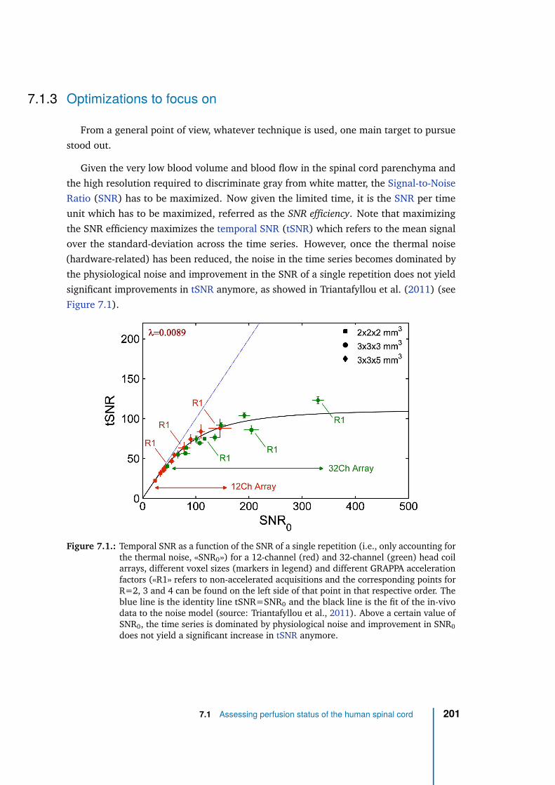
7.1.3 Optimizations to focus on

From a general point of view, whatever technique is used, one main target to pursue

stood out.

Given the very low blood volume and blood flow in the spinal cord parenchyma and

the high resolution required to discriminate gray from white matter, the Signal-to-Noise

Ratio (SNR) has to be maximized. Now given the limited time, it is the SNR per time

unit which has to be maximized, referred as the SNR efficiency. Note that maximizing

the SNR efficiency maximizes the temporal SNR (tSNR) which refers to the mean signal

over the standard-deviation across the time series. However, once the thermal noise

(hardware-related) has been reduced, the noise in the time series becomes dominated by

the physiological noise and improvement in the SNR of a single repetition does not yield

significant improvements in tSNR anymore, as showed in Triantafyllou et al. (2011) (see

Figure 7.1).

Figure 7.1.: Temporal SNR as a function of the SNR of a single repetition (i.e., only accounting forthe thermal noise, «SNR0») for a 12-channel (red) and 32-channel (green) head coilarrays, different voxel sizes (markers in legend) and different GRAPPA accelerationfactors («R1» refers to non-accelerated acquisitions and the corresponding points forR=2, 3 and 4 can be found on the left side of that point in that respective order. Theblue line is the identity line tSNR=SNR0 and the black line is the fit of the in-vivodata to the noise model (source: Triantafyllou et al., 2011). Above a certain value ofSNR0, the time series is dominated by physiological noise and improvement in SNR0

does not yield a significant increase in tSNR anymore.


Therefore, once this point has been reached, the remaining available SNR increase can

be traded for higher acceleration factor to limit geometric distortions due to the long EPI

readout for instance. However, in the case of parallel imaging, the accurate estimation of

the thermal noise in a single repetition («SNR0») requires heavy calculations involving

Monte-Carlo simulations based on measurements of the coil array g-factor map and the

noise covariance matrix as well as access to the reconstruction routine, including the

parallel imaging reconstruction algorithm used as in Triantafyllou et al. (2011).

Increasing field strength linearly increases the SNR efficiency (as explained in sec-

tion 2.3.1) and for human, 7T MRI is the optimum in terms of clinically approved field

strength.

As averaging data increases the SNR by the square root of the number of averages,

one strategy is to acquire as many images as possible in the allocated time. This strategy

is possible for endogenous techniques. For exogenous techniques based on the passage

of the contrast agent in the tissue, acquisition time cannot be traded for SNR. However,

the same target (optimization of SNR efficiency or tSNR) holds. Common rapid imaging

strategies such as cited in section 2.2.2 are therefore generally employed whatever the

perfusion technique. EPI is the most frequently used readout because of its efficient

k-space coverage and low SAR, compared to turbo-flash or turbo-spin-echo readouts for

instance, although preparation and readout are sometimes intimated related such as for

turbo-spin-echo. For exogenous perfusion MRI, it is also important to have a fast readout

as a snapshot image because we are imaging a constantly changing mechanism. However,

EPI is poorly robust to B0 inhomogeneities.

In the two perfusion techniques investigated in this thesis, the sensitivity to perfusion is

obtained through T2 dephasing (direct or indirect): T2 dephasing induced by molecular

displacement in association with diffusion gradients for IVIM or T2/T2* dephasing

induced by susceptibility effects of the contrast agent for DSC. T1-weighted sequences

thus could not be used such as in DCE MRI which are less sensitive for blood flow

estimation. This consequently precludes the use of turbo-flash readouts which provide

great image quality even in the presence of B0 heterogeneity. The challenge here was

therefore to have a fast readout with a signal sensitive to transverse magnetization

dephasing and robust to B0 inhomogeneities. To cope with the high sensitivity of EPI to

B0 inhomogeneities, spin-echo EPI sequences were preferred at first over gradient-echo

EPI (sensitivity to T2 relaxation and mitigation to T2* relaxation). Nonetheless, other

solutions could be considered.

202 Chapter 7

In the case of IVIM, segmented EPI approach could be used (as time is not limited

by the bolus as in DSC). The long echo train length (coming with high resolution) in

single-shot EPI introduces SNR loss due to the T2*-weighted signal decay along readout.

If Nseg is the number of segments, the SNR gained with data averaging in single-shot EPI

(√

Nseg) has to be compared with the SNR gained when reducing the readout by Nseg.

In addition, the reduction of the readout length with segmented EPI offers a reduction

in image distortions, which can be a significant advantage at 7T in the spinal cord but

comes at the expense of longer acquisition times (limited in clinical routine) and a higher

probability of patient motion.

In the case of DSC where the time allocated for acquiring the whole image is limited

by the cardiac cycle (0.6 to 1.5 s), other readout techniques could theoretically be of

interest. Given its increased sensitivity to contrast bolus (T2* weighting) compared to

spin-echo,GRE-EPI is of course a solution of interest if post-processing methods could

be able to correct image distortions. But steady-state free precession sequences, such

as FISP/FFE/GRASS or trueFISP/balanced FFE/FIESTA (vendor-dependent acronyms)

or fast spin-echo sequences, such as RARE/FSE/TSE, could also be considered. Such

sequences use evenly spaced pulses with short TR to maintain a non-null transverse

magnetization or consecutive refocusing pulses to acquire more than one echo after each

90° excitation pulses. Those techniques could provide great image quality in the spinal

cord with very little or no distortions. However, the cardiac gating is challenging with

those sequences and they are limited by SAR at 7T because of their higher number of

pulses compared to EPI. Increasing the repetition time is therefore necessary at 7T which

deteriorates the temporal resolution.

This leads to the benefits and drawbacks of ultra-high field MRI.

7.1.4 Benefits and drawbacks of Ultra-High Field

Benefits and drawbacks of Ultrahigh Field (UHF) MRI have been listed in section 2.3.

Their consequences on our objective will be discussed here.

SNR was increased at 7T with a larger proportion of protons contributing to the signal

compared to 3T, but SNR efficiency was limited by SAR for some subject morphologies

which required more power to properly flip the magnetization in the spinal cord. SAR

restrictions are also proper to the coil design which is different between 3T and 7T.

For IVIM, SAR was less a limitation than for DSC because TR was not restricted. The


limitation was on the minimal TE (because of the diffusion gradients). Nevertheless,

despite the high in-plane resolution used (0.7×0.7 mm2), a tSNR around 11 was obtained

for IVIM (native value, without any processing or averaging), ranging from 9 to 14. It

was slightly lower for DSC due to SAR limitations for some subjects, leading to a tSNR

as low as 5. Excluding subjects with limited coil voltage, tSNR was around 11 for DSC

data, increased to 13 after motion correction and to 22 with an in-plane resolution of

1.04×1.04 mm2 (respectively, 28 after motion correction).

SAR limitations can be alleviated with more appropriate coil array design. The coil

array used in this work is a "first generation" prototype, now commercialized by Siemens

Healthcare with the Terra 7T system but which might benefit from future developments.

The inferior-superior extent of the "relatively optimal" B1 transmit field is currently

limited to 3-4 vertebral levels (depending on the subject’s morphology), and thus needs

to be improved. It is worth noting that parallel transmission (possible with this coil array

but not yet used) is more likely to efficiently improve the B1 transmit field homogeneity

for 7T MRI of the spinal cord. This emerging technology requires a specific expertise

in electromagnetic simulations to ensure that no local SAR hot spots are produced with

the new field distribution using the transmit channels independently. Dieletric pads

placed around the patient’s neck could also help B1 transmit homogeneity but currently

also require ethics approval as they modify the field distribution similarly to a new coil.

Dieletric pads can additionally help mitigating B0 homogeneity, which is also a major

challenge for 7T MRI of the spinal cord.

Indeed, spinal cord imaging at 7T requires strong B0 shimming efforts. Performance

of the automatic Siemens algorithm is highly dependent on the subject and the shimming

ROI. The difficulty with spinal cord is its longitudinal tubular shape. While including

the whole slice in the shimming ROI is advised by high-resolution functional MRI studies

in the brain to mitigate Nyquist N/2 ghost artifacts, the common practice in spinal

cord is to restrict the shimming ROI around the cord in transversal plane in order to

force the algorithm to optimize shimming in spinal cord whatever happens outside it,

potentially enhancing Nyquist N/2 ghost artifacts (as signal in cord includes contributions

from the entire k-space). Some also advise a trade-off between those two approaches

including cervical muscles posterior to the cord in the ROI to feed the algorithm with

more steady tissue. However, the most promising approaches to deal with multiple

sources of B0 inhomogeneity in the spinal cord are dynamic shimming — update shim

settings according to the slice position — or real-time shimming — update shim settings

according to the signal of a sensor, e.g. respiratory belt, provided prior calibration. As

204 Chapter 7

described in section 2.3.3, those approaches require specific coil arrays and amplifiers

capable of fast shim updates. If no such technology is available on 7T systems yet, data

can be corrected for dynamic fluctuations post-acquisition as proposed in Vannesjo et al.

(2019) where breathing-induced phase offset is corrected before reconstruction, or as

proposed in this thesis for DSC data, where breathing frequencies are filtered out in

temporal signal. However, if EPI trajectory errors can be corrected, dephased signal

cannot be recovered with such approaches. Moreover, the latest approach is only valid

for applications looking at signal evolution in time and interested in frequencies different

from the breathing frequencies (∼0.25 Hz). Effect of breathing on IVIM data has not been

investigated but it is expected to be filtered out through the averaging across repetitions.

Furthermore, previous work have assumed a linear relationship between the pressure

sensor from the respiratory bellows and the time-varying B0 field. But as speculated by

Gelderen et al. and supported by most studies in spinal cord (Bianciardi et al., 2014;

Vannesjo et al., 2018; Topfer et al., 2018), there may be field variations that are not

linearly related to the abdomen or chest position as measured by the respiratory bellows.

Indeed, a field probe placed next to the chest showed only partial correlation between

dynamic field variations and respiratory sensor (Boer et al., 2012). As explained by

the authors, the breathing mechanism has two degrees of freedom: one permitted by

the diaphragm and the other by the intercostal muscles. The lungs expansion during

breathing can therefore happen exclusively through the motion of the central tendon of

the diaphragm with motionless lower ribs (belly or diaphragmatic breathing), expanding

the cavity downwards. Or it can exclusively happen with the motion of the lower ribs,

the central tendon of the diaphragm staying still to expand the thoracic cavity laterally

and upwards (costal breathing). Even if those two forms usually happen in conjunction

(diaphragm contraction followed by intercostals contraction), the resulting B0 variations

cannot be fully characterize with the information of a respiratory bellows only. Experts

even distinguish more than two types of breathing. Moreover, the breathing mode

changes across individuals, which could explain the differences in signal steadiness

observed across patients in the DSC study. Breathing types involving upwards expansion

of the thoracic cavity is more likely to disturb the field in the cervical region.

As a matter of fact, increased sensitivity to B0 variations at 7T is a major issue

for spinal cord imaging. If breathing-induced variations can be approximated with a

respiratory sensor, other physiological contributions to B0 variations in spinal cord such

as swallowing or fluid motion are more difficult to characterize. Indeed, even though

a quiescent period of the CSF exists, the proximity of the trachea and of large arteries


and veins (aorta, superior vena cava, subclavian arteries and veins) containing fluid in

constant motion, might induce additional field variations in the cervical cord. Given the

small dimensions of the cord and the low sought-after perfusion signal, very little field

variations can be significant. By way of example, it is common to see Nyquist N/2 ghost

and GRAPPA calibration-related artifacts exacerbated during the passage of the contrast

agent in MR angiography (Irwan et al., 2007). It was also observed in some patients in

the DSC study. Coming in the imaging field-of-view through multiple inlets in the neck,

the contrast agent modifies the susceptibility in multiple points, which, depending on the

shimming, might disturb the B0 field with variable consequences on the image quality

(since all spins in the field-of-view contribute to the image quality), in particular due to

GRAPPA miscalibration. Hopefully, with the current coil design and its limited transmit

and receive field coverage, signal coming from vessels on the anterior side of the neck is

mitigated. Nonetheless, robustness of the GRAPPA calibration should be fixed for future

studies

Finally, one major advantage of UHF MRI for Dynamic Susceptibility Contrast imaging

is the increased relaxivities r2 and r∗

2 of gadolinium-based contrast agents. As described in

section 2.4.1, the increase of R2 with field strength is theoretically null but was measured

in practice. It was one benefit of working at 7T for bolus detection. However, the full

potential of UHF for contrast agent sensitivity was not leveraged in this work. Indeed,

the increase in R∗

2 from 7T to 3T in much higher than for R2. But it is so increased that

it becomes a problem for GRE-EPI in the spinal cord, leading to large signal dropout

especially on the anterior side of the cord and at the vicinity of intervertebral disks.

Robustness to B0 inhomogeneity is also reduced with GRE-EPI. For these reasons and

with an objective to produce maps of perfusion, spin-echo-EPI was preferred for the DSC

study. In this regard, the balance between the benefit of the increased r2 and drawbacks

of the higher sensitivity to physiological noise at 7T has to be compared with the balance

between the benefit of the higher sensitivity of GRE-EPI to contrast agent (with respect

to spin-echo-EPI) and the drawback of increased noise at 3T. “Food for thought” is

presented in Table 7.1. The question is to define the relative significance of those features

which are highly interdependent. Significance might also depend on the application.

For instance, in this work, only transverse slices were considered with the purpose to

depict the perfusion difference between gray and white matter. However, sagittal slices

might be of greater interest to assess the longitudinal extent of ischemia induced by

compression in Degenerative Cervical Myelopathy (DCM) patients. Although distinction

between gray and white matter would be partially lost because of partial volume effects

with relatively thick slices (necessary for a sufficient SNR), sagittal acquistions would

206 Chapter 7

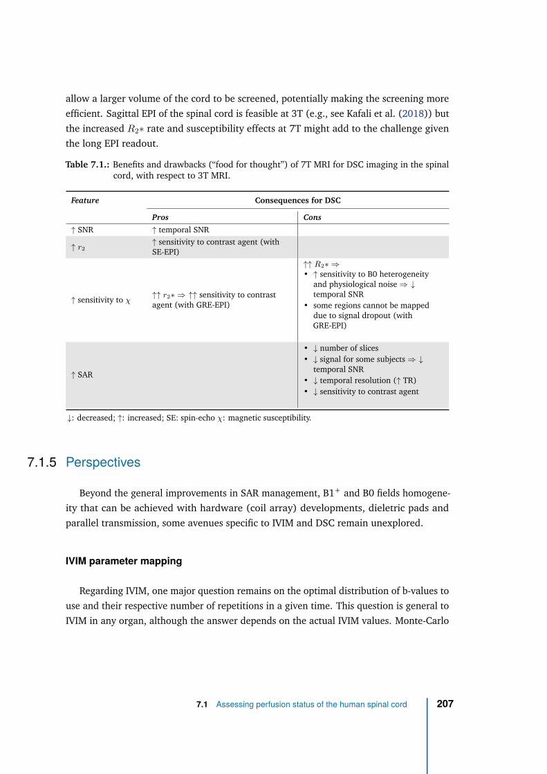
allow a larger volume of the cord to be screened, potentially making the screening more

efficient. Sagittal EPI of the spinal cord is feasible at 3T (e.g., see Kafali et al. (2018)) but

the increased R2∗ rate and susceptibility effects at 7T might add to the challenge given

the long EPI readout.

Table 7.1.: Benefits and drawbacks (“food for thought”) of 7T MRI for DSC imaging in the spinalcord, with respect to 3T MRI.

Feature Consequences for DSC

Pros Cons

↑ SNR ↑ temporal SNR

↑ r2

↑ sensitivity to contrast agent (withSE-EPI)

↑ sensitivity to χ↑↑ r2∗ ⇒ ↑↑ sensitivity to contrastagent (with GRE-EPI)

↑↑ R2∗ ⇒

• ↑ sensitivity to B0 heterogeneityand physiological noise ⇒ ↓

temporal SNR• some regions cannot be mapped

due to signal dropout (withGRE-EPI)

↑ SAR

• ↓ number of slices• ↓ signal for some subjects ⇒ ↓

temporal SNR• ↓ temporal resolution (↑ TR)• ↓ sensitivity to contrast agent

↓: decreased; ↑: increased; SE: spin-echo χ: magnetic susceptibility.

7.1.5 Perspectives

Beyond the general improvements in SAR management, B1+ and B0 fields homogene-

ity that can be achieved with hardware (coil array) developments, dieletric pads and

parallel transmission, some avenues specific to IVIM and DSC remain unexplored.

IVIM parameter mapping

Regarding IVIM, one major question remains on the optimal distribution of b-values to

use and their respective number of repetitions in a given time. This question is general to

IVIM in any organ, although the answer depends on the actual IVIM values. Monte-Carlo


simulations as employed in the IVIM study can theoretically address this question by

testing all possible combinations and keep the one resulting in the lowest error but in

practice, the number of calculations is way too large to be performed in a reasonable

time (≤ 1 month, even using the high computational resources of Aix-Marseille University

Mesocentre). Another method is to calculate the Cramer-Rao lower bounds. In any

problem involving the fit of a model to measurements to estimate some parameters, the

Cramer-Rao lower bound defines the theoretical lower uncertainty that can be obtained

on the estimated parameter with the given measurements. It has an analytical expression

based on the signal representation as a function of the b-value and the corresponding

Fisher matrix F calculated as follows:

Fpjpk=

1

σ2

N∑

i=0

ni∂S(bi)

∂pj

∂S(bi)

∂pk

where p are the parameters (fIV IM , D∗, D and Sb=0), σ is the noise standard-deviation,

N + 1 is the number of unique b-values, ni is the number of repetitions for the b-value bi

resulting in signal S(bi). The SNR can be plugged into the equation as σ = Sb=0/SNR.

The SNR value in input should be the SNR obtained when b=0 and for a single repetition.

The increase in SNR with averaging is accounted for with the factor ni. Note that a

Gaussian noise is therefore assumed.

The Cramer-Rao lower bound for parameter p is defined by the corresponding diagonal

element of the inverse of the Fisher matrix according to:

σp2 ≥ (F −1)pp

where σp2 is the variance of the estimated parameter p with the given distribution and

the expected actual parameter values p. An error function to be minimized can be defined

for example as:

ǫ =

√(F −1)fIV IM fIV IM

fIV IM+

√(F −1)D∗D∗

D∗

Such error function would seek to minimize the uncertainty on fIV IM and D∗ whatever

the uncertainty on D and Sb=0 is. The global strategy would be to calculate ǫ for all

distributions possible and take the distribution minimizing it. To go further, given that

the actual parameter values are likely to vary depending on the tissue, we would need to

evaluate ǫ across a range of expected parameter values and take, for example, the average

or maximum error to rate the given distribution. Even if this approach also involves a large

number of calculations, it is faster than the Monte-Carlo simulations approach because

208 Chapter 7



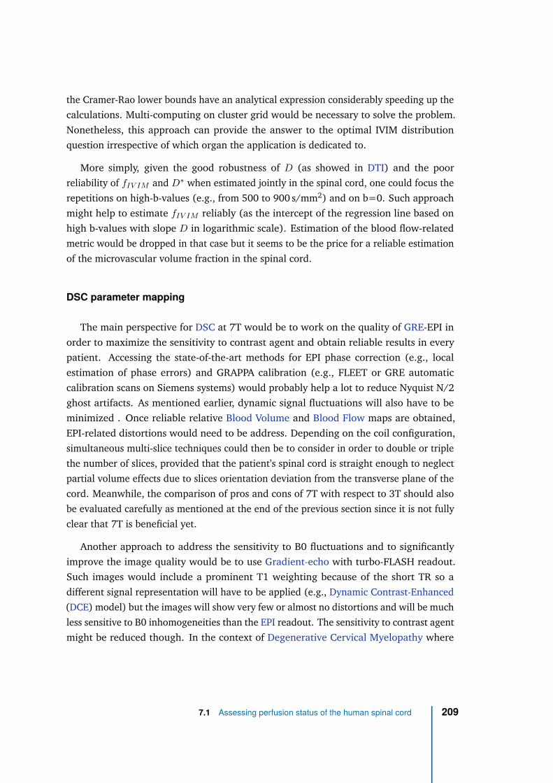
the Cramer-Rao lower bounds have an analytical expression considerably speeding up the

calculations. Multi-computing on cluster grid would be necessary to solve the problem.

Nonetheless, this approach can provide the answer to the optimal IVIM distribution

question irrespective of which organ the application is dedicated to.

More simply, given the good robustness of D (as showed in DTI) and the poor

reliability of fIV IM and D∗ when estimated jointly in the spinal cord, one could focus the

repetitions on high-b-values (e.g., from 500 to 900 s/mm2) and on b=0. Such approach

might help to estimate fIV IM reliably (as the intercept of the regression line based on

high b-values with slope D in logarithmic scale). Estimation of the blood flow-related

metric would be dropped in that case but it seems to be the price for a reliable estimation

of the microvascular volume fraction in the spinal cord.

DSC parameter mapping

The main perspective for DSC at 7T would be to work on the quality of GRE-EPI in

order to maximize the sensitivity to contrast agent and obtain reliable results in every

patient. Accessing the state-of-the-art methods for EPI phase correction (e.g., local

estimation of phase errors) and GRAPPA calibration (e.g., FLEET or GRE automatic

calibration scans on Siemens systems) would probably help a lot to reduce Nyquist N/2

ghost artifacts. As mentioned earlier, dynamic signal fluctuations will also have to be

minimized . Once reliable relative Blood Volume and Blood Flow maps are obtained,

EPI-related distortions would need to be address. Depending on the coil configuration,

simultaneous multi-slice techniques could then be to consider in order to double or triple

the number of slices, provided that the patient’s spinal cord is straight enough to neglect

partial volume effects due to slices orientation deviation from the transverse plane of the

cord. Meanwhile, the comparison of pros and cons of 7T with respect to 3T should also

be evaluated carefully as mentioned at the end of the previous section since it is not fully

clear that 7T is beneficial yet.

Another approach to address the sensitivity to B0 fluctuations and to significantly

improve the image quality would be to use Gradient-echo with turbo-FLASH readout.

Such images would include a prominent T1 weighting because of the short TR so a

different signal representation will have to be applied (e.g., Dynamic Contrast-Enhanced

(DCE) model) but the images will show very few or almost no distortions and will be much

less sensitive to B0 inhomogeneities than the EPI readout. The sensitivity to contrast agent

might be reduced though. In the context of Degenerative Cervical Myelopathy where


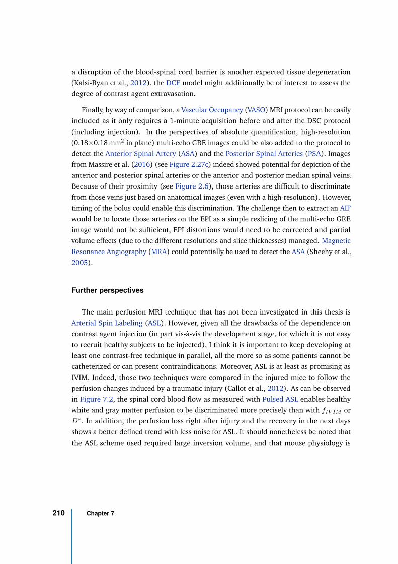
a disruption of the blood-spinal cord barrier is another expected tissue degeneration

(Kalsi-Ryan et al., 2012), the DCE model might additionally be of interest to assess the

degree of contrast agent extravasation.

Finally, by way of comparison, a Vascular Occupancy (VASO) MRI protocol can be easily

included as it only requires a 1-minute acquisition before and after the DSC protocol

(including injection). In the perspectives of absolute quantification, high-resolution

(0.18×0.18 mm2 in plane) multi-echo GRE images could be also added to the protocol to

detect the Anterior Spinal Artery (ASA) and the Posterior Spinal Arteries (PSA). Images

from Massire et al. (2016) (see Figure 2.27c) indeed showed potential for depiction of the

anterior and posterior spinal arteries or the anterior and posterior median spinal veins.

Because of their proximity (see Figure 2.6), those arteries are difficult to discriminate

from those veins just based on anatomical images (even with a high-resolution). However,

timing of the bolus could enable this discrimination. The challenge then to extract an AIF

would be to locate those arteries on the EPI as a simple reslicing of the multi-echo GRE

image would not be sufficient, EPI distortions would need to be corrected and partial

volume effects (due to the different resolutions and slice thicknesses) managed. Magnetic

Resonance Angiography (MRA) could potentially be used to detect the ASA (Sheehy et al.,

2005).

Further perspectives

The main perfusion MRI technique that has not been investigated in this thesis is

Arterial Spin Labeling (ASL). However, given all the drawbacks of the dependence on

contrast agent injection (in part vis-à-vis the development stage, for which it is not easy

to recruit healthy subjects to be injected), I think it is important to keep developing at

least one contrast-free technique in parallel, all the more so as some patients cannot be

catheterized or can present contraindications. Moreover, ASL is at least as promising as

IVIM. Indeed, those two techniques were compared in the injured mice to follow the

perfusion changes induced by a traumatic injury (Callot et al., 2012). As can be observed

in Figure 7.2, the spinal cord blood flow as measured with Pulsed ASL enables healthy

white and gray matter perfusion to be discriminated more precisely than with fIV IM or

D∗. In addition, the perfusion loss right after injury and the recovery in the next days

shows a better defined trend with less noise for ASL. It should nonetheless be noted that

the ASL scheme used required large inversion volume, and that mouse physiology is

210 Chapter 7

different from human’s (blood flow approximately 5-fold higher, larger GM/WM ratio

potentially associated with a larger blood volume and a different blood supply).

Figure 7.2.: Comparison between IVIM and ASL in the monitoring of perfusion changes in theinjured mice (from Callot et al. (2012)). Graphs (a) and (b) show the evolution ofIVIM parameters post-injury, with a comparison to healthy values (N=5) while (c)shows the evolution of the spinal cord blood flow (SCBF) as measured by continuousASL.

As described in the first chapter (see subsection 2.4.4), two different attempts to apply

ASL to human spinal cord were reported in conference proceedings (Nair et al., 2010;

Girard et al., 2013) but the poor reliability of the results discouraged more developments.

However, at 3T (Nair et al., 2010), continuous ASL was used whereas the most efficient

tagging scheme as advised in the ASL consensus paper (Alsop et al., 2015) is pseudo-

continuous ASL. And indeed, this tagging scheme showed better sensitivity to perfusion

at 1.5T (Girard et al., 2013) as illustrated by the obtained signal difference between tag

and control images (Figure 7.3).

Figure 7.3.: Signal in human cord from control and tag images using PCASL at 1.5T (from: Girardet al. (2013))

In light of those results, PCASL would be worth further developments at 3T and even

7T. Indeed, if it appears technically challenging due to the SAR limits at 7T, ASL has been

successfully applied at 7T in brain (Ghariq et al., 2012; Wang et al., 2015; Gardener

et al., 2015; Pfeuffer et al., 2002). One advantage of ASL compared to DSC is that a


longer acquisition time can be traded for SNR and alleviation of SAR limits. However,

ASL requires the identification of the best arteries to tag with adequate transit time (prior

MRA could be beneficial for a patient-specific ASL protocol), and above all, more optimal

cervical coil design or parallel transmission to provide efficient labeling. Many challenges

for the future!

7.2 Biomechanical modeling of DCM-like spinal cord

compression

7.2.1 Achievements

Useful features of the study

The first important feature of the biomechanical study of degenerative compressions

performed in the context of this thesis lies in the definition of a quantitative value for

the compression threshold beyond which substantial tissue damage is likely to occur

and induce myelopathy. This compression threshold of 30% in Cross-Sectional Area

has been determined based on both previous morphological literature data and a DCM

patient cohort. It was actually consistent with several other finite element simulations

of chronic spinal cord compression which particularly reported a significant increase of

the constraints above this value (Kato et al., 2010; Kim et al., 2013; Khuyagbaatar et al.,

2015). It was additionally observed in mice under chronic compression that the number

of motoneurons in gray matter started to decrease above the same threshold value (30%

compression in CSA) (Baba et al., 1996; Baba et al., 1997), even though the connection

with human has to be made with caution since the gray matter/white matter ratio is

higher in the mouse (∼50% versus 20%). Nevertheless, this compression value really

stands out as a critical threshold.

The quantitative definition of a compression threshold is essential for the compar-

ison across different compression patterns. In most studies, simulations and analysis

were performed with an arbitrary compression degree or multiple degrees, which makes

the interpretation of the results and their validity with respect to observed symptoms

complicated. It is also possible that, in practice, the critical compression value changes

212 Chapter 7

depending on the compression type (median diffuse, median acute, lateral, circumferen-

tial). More data are necessary to define a myelopathic compression threshold for each

compression type.

The second interesting feature compared to previous studies looking at chronic de-

generative compression is the anatomic fidelity of the model. Indeed, given the large

variability in compression patterns as well as in the symptoms nature and severity ob-

served in DCM, the anatomy appears as a critical factor. For instance, the anatomy

of the vertebrae, and in particular the height between the lamina (which clamps the

cord on the posterior side) and the intervertebral disk compressing the cord against it,

induced normal stress along the inferior-superior axis and shear stress in those planes.

The anatomy of ligaments and intervertebral disk (position, size, shape) also played an

important role which simple artificial shapes (e.g., perfect parallelepiped, tetrahedron)

might not account for in previous studies.

The third important feature of the finite element analysis carried out in this thesis is

the automatic pipeline for a quantitative analysis of constraints along time steps, across

anatomic spinal cord Region-Of-Interest (ROI) and along any dimension. To the best of

my knowledge, none of the previous finite element study of chronic compression looked

at the induced constraints in such a quantitative manner. The most common approach

is to visually compare constraint maps. However, such approach intrinsically limits the

extent of the analysis and results to be tabulated. It will inevitably miss some aspects of

the constraint patterns. The quantitative set up has the power to reveal subtle differences.

In a view to relate mechanical constraints to tissue perfusion and to explore the time

scale of the events, such analysis is essential.

Important findings

Based on this biomechanical study and on its classification across compression types

(consistent with Nishida et al. (2012) and Khuyagbaatar et al. (2015)), the median

diffuse type would be more detrimental to the tissue, supporting the findings of Nishida

et al. (2012) and Khuyagbaatar et al. (2015). The magnitude of the induced stresses

was higher for this type. The predominant stress was normal or "directional" stress while

shear stress was marginal. Based on the simulated material properties, the main affected

region is by far the gray matter which is consistent with the motoneurons death observed

in compressed mouse spinal cord (Baba et al., 1996; Baba et al., 1997) and with the

reported gray matter infarction in DCM patients (Fehlings et al., 1998). The secondly

7.2 Biomechanical modeling of DCM-like spinal cord compression 213

affected regions would then be the anterior and posterior regions, which actually result

in a global injury pattern affecting all regions in the sagittal plane, even for the lateral

compression type. This is intuitively explained by the main anterior-posterior direction of

the applied loading. However, the observed resulting stresses could not directly explain

the corticospinal tracts demyelination reported in clinicopathologic studies of DCM

(Ogino et al., 1983). According to Fehlings et al. (1998) based on experimental studies in

dogs of Shimomura et al. (1968) Gooding et al. (1975), ischemia would exacerbate the

pathological effects of mechanical compression and make the corticospinal tracts more

vulnerable than others to injury. Consequently, mechanical stress only might not be able

to explain the tissue degeneration observed in corticospinal tracts of DCM patients, hence

the benefit of coupling biomechanical simulation to perfusion measurements.

7.2.2 Model validity

The final concern as in any biomechanical study is the validity of such simulations.

Model validation

Model validation in biomechanics applied to human is complex due to the in-vivo

nature of the problem and the legal/ethical/moral impossibility to perform experimental

measurements.

The Spine Model for Safety and Surgery (SM2S) benefits from the conjoint work of

several research groups associated within an international laboratory (the iLab-Spine). As

a consequence, the model benefits from the multiple validation studies which have been

carried out since 2009. Those mainly focused first on vertebrae and ligaments and later,

on integration of the spinal cord. Nevertheless, fewer validation studies investigated

the gray and white matter properties (Fournely et al., 2020). As a matter of fact, the

in-vivo characterization of spinal cord tissue properties is extremely challenging as they

immediately start to change once harvested. Very recently, ex-vivo measurements were

performed using nano-indentation within the iLab-Spine but results are not published

yet. This work will certainly help the validation and refinement of the model. In the

meantime, values derived from the literature for bovine tissue (Ichihara et al., 2001;

Ichihara et al., 2003) were used for the simulations. Sensitivity analysis — i.e. repeating

the study with varied parameters (e.g., different values of gray and white matter tangent

214 Chapter 7

modulus) — would evaluate the dependency of the obtained results in the gray and white

matter parameters. Such study would be interesting first because the gray and white

matter parameters of the human spinal cord are barely known and secondly because they

are likely to change with age, ischemia and tissue degeneration.

Similar analysis could also be performed on other simulation parameters which were

arbitrarily set: the duration of the simulation, the mesh resolution, the compression

velocity, the proportion of asymmetry for lateral and circumferential types, the impactor

sharpness for all types, ..., are many parameters that could affect the results. Morphology-

dependent parameters (vertebral body height, spinal cord occupation ratio in the spinal

canal, etc.) can be added to this list.

Relating constraints to symptoms

The list of influencing parameters can be very long. Multiplying the number of

simulation designs increases the number of simulation to perform by the number of

parameters and their respective values, quickly making the mission very tedious.

One approach to relate the mechanical stress from those simulations to patients’

symptoms would be to classify symptoms according to the compression types. However,

it requires (1) that patients can all be classified within a single type (e.g., multi-level

compression with different compression types across levels are possible), (2) that common

symptoms stand out within each compression type and (3) that differences in symptoms

across types emerge. Those differences then will have to be explored in light of the

biomechanical simulations.

Another approach is to design the simulation so as to best represent what is happening

to the patient, also referred as patient-specific simulations. This approach is more techni-

cally challenging. First the model will need to be warped to the dimensions of the patient

based on general anatomic details (vertebral body height, spinal canal diameter, cord

diameter). This step can be performed by means of 3D anatomical MRI of the patient

and anatomical landmarks manually defined by the user. For this step, care should be

taken to minimize the contribution of degenerations in the warping. In a second step, the

displacement of the degenerated anatomical entities (e.g., intervertebral disk, ligament)

will need to be measured on the MRI and set in the simulation. This procedure can be

made quasi-automatic to minimize manual user intervention, reducing the likelihood of

errors and saving time. Although more technically challenging, this approach will be

7.2 Biomechanical modeling of DCM-like spinal cord compression 215

much closer to the actual constraints that applies in the patient. This approach has the

potential to address the question of the contribution of the mechanical constraints to the

symptoms of DCM.

7.2.3 Perspectives

Direct perspective for this work would be to overcome the limitations of the study.

First, simulations were performed on a very limited length of the spine (C4 to C6)

and top and bottom vertebrae were fixed. Including more segments, or even the whole

spine (although not computationally efficient) would eliminate any potential bias on the

constraint distribution along the inferior-superior axis caused by this artificial crop. Also

in this respect, fixing all vertebrae is also advised as they are expected to be maintained

by the neck and back muscles. This will additionally help reach the compression threshold

faster for every type.

Secondly, although many parameters might have an effect on simulation results, it

would be interesting to identify a few (simulation duration, mesh, compression velocity)

and analyze the sensitivity of the results to those parameters by way of validation. The

initial spinal canal diameter has been reported as a critical underlying factor in the

eventual development of DCM (Burrows, 1963; Murone, 1974). Its effect should also be

considered but it requires a complex reshaping of the model.

Thirdly, given the long time scale which the compression process develops over, it is

speculated, based on cortical studies specific to DCM, that neural plasticity would allow

the tissue to adapt and compensate for compression (Tam et al., 2010; Holly et al., 2007).

This means that the tissue would have time to relax the constraints (or a part of it) during

chronic compression. Such process would also be relevant to model for a more realistic

and accurate analysis of the constraints along the compression process.

Last but not least, investigating the effect of mechanical properties change with tissue

degeneration along compression would provide more insights into the understanding

of the biomechanics of the pathology. Such investigations would imply to first estimate

how the tissue properties vary with neuronal loss, demyelination, inflammation and

blood-spinal cord barrier disruption which might not be trivial given the challenges

already faced in the estimation of healthy gray and white matter properties.

Next step would be to include compression at multiple levels as it is often observed.

The effect of the vertebral body height and distance between two compressed levels will

thus have a strong meaning as the effects of multiple compressions could meet in the same

216 Chapter 7

place. In that regard, multi-level versus single-level compressions might have significant

consequences on the patient’s symptoms, and a step forward towards patient-specific

simulations would be taken. Nonetheless, the experimental plan and analysis for such

study along with validation or sensitivity analysis is very complex given the number of

degrees of freedom (compression types, number of compressed levels, distance between

levels).

Furthermore, including strain in the study would refine the analysis. Indeed, Doppman

(1975) observed, inter alia, that flattening the cord (stretching it to left and right side)

using a balloon catheter in the monkey disrupted the perfusion in intramedullary arteries

running transversely because of the elongation and narrowing applied. This finding

suggests that the disruption of perfusion rather comes from the strain applied to the

vascular network than from the stress applied to the tissue. It also suggests that including

arteries and veins in the SM2S might be necessary to actually grasp the compression

mechanisms leading to ischemia. In the first place, arteries and veins can be modeled

very simply as straight tubes such as proposed in Alshareef et al. (2014). Magnetic

Resonance Angiography (MRA) images of the spinal cord could further be used to design

more sophisticated representations of the spinal cord vascular network if necessary. Such

feature would take a further step in addressing the question about whether the ischemia

is rather due to arterial supply interruption or to capillary network alteration within the

cord parenchyma.

7.3 Relating perfusion and mechanical constraints in

chronic spinal cord compression

As enunciated in introduction and objectives, this PhD is part of a global project

aiming to relate pathophysiological deficit measured with MRI to mechanical constraints

simulated with biomechanical models in the context of degenerative spinal cord compres-

sion to guide surgery and help identifying risk and prognosis factors. This PhD work was

particularly conducted with the perspective of establishing a quantitative relationship

between mechanical constraints and induced ischemia, which could allow neurosurgeons

to define threshold criteria and assist them in surgical decisions.

However, despite the multiple achievements resulting from this work, this objective

has not been reached yet. A promising method to map human spinal cord perfusion

7.3 Relating perfusion and mechanical constraints in chronic spinal cord

compression

217

(DSC) has been identified and its feasibility at 7T was investigated. But obtained per-

fusion map still lack reliability to confidently depict ischemia in DCM patients. On the

biomechanics side, realistic simulations of typical DCM compression patterns could be

designed and an analysis pipeline was set up to quantitatively investigate the constraints

distribution in spinal cord along compression process, along the spinal cord and across

spinal pathways. But given the large variability of DCM presentations (compression

patterns and symptoms), those simulations still need to get closer to the actual pattern of

compression to relate resulting constraints to symptoms. Reliability of the results also

requires verification for example through sensitivity analysis on the parameters likely to

vary.

Without method for mapping, one could imagine to quantify perfusion parameters in

the whole cord (or in a large ROI within the cord, at the compression site for instance) in

a cohort of patients, along with their respective anatomical MRIs. Then, those patients

would be classified into the four simulated compression types (median diffuse, median fo-

cal, lateral, circumferential). Provided that differences in perfusion across types emerges,

one would then try to explain them based on the results of the biomechanical simulations.

However, given the large number of parameters the simulations depend on, this might be

a highly biased method subject to much larger approximations than the subtle changes

likely to be caused by normal morphological variations.

Indeed, the observed compression pattern in DCM varies a lot (type of compression,

affected levels, number of affected levels, degree of compression). Distribution of

constraints and ischemia within cord is directly related to the compression pattern. For

these reasons and as mentioned earlier, I would advise instead to opt for an approach

focused on the individual case, that is patient-specific approach. Those are also the reason

why a mapping of perfusion indices (instead of a global index value for a large region) is

interesting. In the first place and as development stage, high-resolution 2D transverse

acquisitions were preferred so as to use the difference between gray and white matter

perfusion as a validation index for the obtained perfusion maps. Ideally such acquisitions

would include more slices (≥10) so as to sample and cover both compression area(s) and

healthy tissue rostro-caudally, hence giving a better picture of the effect of compression

on the perfusion distribution (combined with an assessment of microstructural alteration

of course). On the biomechanics side, it would be important to stick the simulation

design to the individual patient’s compression pattern especially in the inferior-superior

direction. Moreover, in order to address the question about the level in vascular network

of the perfusion disruption induced by compression (rather on arterial/vein vascular

218 Chapter 7

network or within capillary network), the main arteries and veins should be included in

the SM2S, even as simple straight tubes as in Alshareef et al. (2014).

In the context of degenerative spinal cord compression, mechanical constraints induced

by compression can be simulated, perfusion deficit could be measured, symptoms can

be assessed and all of them could possibly be related. But in this chain of events,

right in-between perfusion deficit and symptoms, microstructural damages secondary

or concomitant to ischemia should also be evaluated using advanced MRI techniques,

such as diffusion MRI, magnetization transfer-based techniques and/or relaxometry MRI

— as currently developed at the CRMBM (see Massire et al. (2016), Taso et al. (2016),

and the article under revision from Baucher et al. about T1 mapping for microstructural

assessment of the cervical spinal cord in the evaluation of patients with degenerative cervical

myelopathy) —, or using a combination of those techniques (multi-parametric MRI) as

proposed in Martin et al. (2018). Putting those techniques altogether is one of the

iLab-Spine’s challenges.

Finally, a completely different approach to relate ischemia and microstructural al-

terations to biomechanical tissue properties but still coupling biomechanics to MRI, is

Magnetic Resonance Elastography (MRE). As described in chapter 2 (section 2.6.2), this

technique enables the shear modulus of the tissue to be measured in-vivo. It was applied

in the cervical spinal cord at 1.5T in a preliminary study (Kruse et al., 2009). However,

with the proposed driver, displacements in the order of 200 µm were identified, which

could correspond to intrinsic bulk motion. In addition, if preliminary stiffness measure-

ments could be extracted, these showed large variations across the cord and could only

be valid for a global assessment. Once further improved, this technique could potentially

be a promising alternative to estimate the expected change of gray and white matter

mechanical properties with aging and tissue degeneration, with a view to investigate the

effects of such changes on finite element simulation results.

7.3 Relating perfusion and mechanical constraints in chronic spinal cord

compression

219

General conclusion 8Degenerative spinal cord compression involves mechanical constraints and perfusion

deficit in the spinal cord, which induce an inflammatory reaction resulting in neuronal

and oligodendroglial death and eventually myelopathy. Indeed, Degenerative Cervical

Myelopathy (DCM) is a common spinal cord disorder in elderly population. If the chain of

pathological events seems consistent with clinical observations and experimental findings,

little is known about the modality of action of each pathological process, their respective

contribution and interactions, as well as the timescale of the processes. As a consequence,

progression of the pathology is difficult to monitor and predict. Moderate/severe DCM are

treated with decompression surgery to limit neurological deterioration but management

of mild DCM is controversial: non-operative treatments (cervical collars or physiotherapy)

with periodic monitoring of symptoms are often preferred over surgery. This PhD work is

part of a global project aiming at exploring and characterizing the different processes

involved in degenerative spinal cord compression.

The first part of the thesis was dedicated to MR technique developments for measure-

ment of spinal cord perfusion, which could ultimately be used by clinicians to assess

the severity of the disease. Quantifying perfusion in the human spinal cord reliably is

extremely challenging as evidenced by previous attempts from different research groups.

Spinal cord is small, its perfusion is low (≤5% of tissue volume) and its vascular network

is complex. Tissue perfusion comes from multiple arteries, from bottom to top with a

limited number of branches running transversely (radicullomedullary arteries) feeding

the smaller arteries (Anterior Spinal Artery and Posterior Spinal Arteries) and at variable

levels. A high SNR is therefore essential to perform reliable measurements. The benefits

of 7T MRI, on the road to clinics, were engaged.

The first investigated technique was Intra-Voxel Incoherent Motion (IVIM). Although

interesting for its independence from Arterial Input Function and its additional estimation

of the diffusion coefficient for microstructural assessment, this technique showed poor

reliability in the spinal cord at the individual level despite a large number of averages. The

higher perfusion of the butterfly-shaped gray matter could only be clearly revealed after

an averaging across slices and subjects. The bi-exponential signal representation of IVIM

221

is indeed speculated to be too sensitive to physiological noise in the human spinal cord

at 7T at the individual level. The second investigated technique, Dynamic Susceptibility

Contrast (DSC), which requires injection of a gadolinium-based contrast agent, showed

more promising results. Known sources of physiological noise were addressed with

cardiac gating and identification of breathing-induced signal fluctuations. Well-defined

relative Blood Flow and Blood Volume maps were obtained in healthy subjects with

in-plane resolution of 0.74×0.74 mm2. Results were more mitigated in case of suspected

perfusion deficit as accounted for by DCM patients. The lack of sensitivity of the spin-

echo sequence to R2 change with contrast compared to gradient-echo sensitive to R∗

2 is

incriminated. The poor robustness of the current static/dynamic B0 shimming routine on

7T whole-body human systems seems also a major source of temporal instability. Benefits

of the currently available technology for spinal cord MRI at 7T needs to be evaluated

against the available technologies at 3T for such an application. Whatever technique or

field strength is used, SNR efficiency is the key.

The second part of the thesis explored the pathological processes of DCM from an

anatomical and biomechanical point of view. The detailed anatomy of the finite element

Spine Model for Safety and Surgery (SM2S) was employed to simulate the constraints

induced by typical DCM compressions. Despite the high variability of compression

patterns across patients, some standards were extracted from literature and from a cohort

of 20 patients. Hence, a 30% reduction in Cross-Sectional Area appeared as a consistent

critical threshold beyond which cell loss and myelopathy occur. The most frequently

affected is C5-C6 and four transverse compression types were selected for simulation

design: median diffuse, median focal, lateral and circumferential. An automatic pipeline

for quantitative analysis of the constraints across compression process, along spinal cord

length and across spinal pathways was set up. Based on induced stress, the median

diffuse compression type would be the most detrimental. Higher stress in gray matter

was in agreement with reported gray matter infarction in DCM patients and motoneuron

loss but demyelination of corticospinal tracts could not be explained by directly induced

stress only. However, sensitivity of those results to simulation parameters need to be

evaluated and strain should be included in the analysis.

In the perspective to investigate the relationship between simulated mechanical con-

straints and perfusion deficit, patient-specific simulation design and perfusion assessment

appeared necessary in front of the large inter-individual variability of compression pat-

terns and symptoms. Such achievements would provide the clinicians with more tools

to monitor the disease progression and optimally manage mild DCM. Furthermore, they

222 Chapter 8

would open the door to new knowledge on the acceptable and non-acceptable constraints

values for the spinal cord tissue integrity, with a large number of applications in the

scope.

223

Publications, communications

and international commitments

9

Journal articles

Published

• Lévy, Simon, Stanislas Rapacchi, Aurélien Massire, Thomas Troalen, Thorsten

Feiweier, Maxime Guye, and Virginie Callot. “Intravoxel Incoherent Motion at

7 Tesla to Quantify Human Spinal Cord Perfusion: Limitations and Promises.”

Magnetic Resonance in Medicine, February 14, 2020, mrm.28195. https://doi.

org/10.1002/mrm.28195

• Lévy, Simon, Guillaume Baucher, Pierre-Hugues Roche, Morgane Evin, Virginie

Callot, and Pierre-Jean Arnoux. “Biomechanical comparison of spinal cord

compression types occurring in Degenerative Cervical Myelopathy.” Clinical

Biomechanics, accepted for publication on September 3, 2020.

• Lévy, Simon, Pierre-Hugues Roche, and Virginie Callot. “Feasibility of spinal

cord perfusion mapping using Dynamic Susceptibility Contrast imaging at 7T:

preliminary results and identified guidelines.” Magnetic Resonance in Medicine,

accepted for publication on September 23, 2020.

Under review

• Baucher, Guillaume, Henitsoa Rasoanandrianina, Simon Lévy, Lauriane Pini, Lucas

Troude, Pierre-Hugues Roche, and Virginie Callot. “T1 mapping for microstruc-

tural assessment of the cervical spinal cord in the evaluation of patients with

degenerative cervical myelopathy.” American Journal of Neuroradiology, recom-

mended for major revision on July 1, 2020.

225



Communications at conferences and workshops

Peer-reviewed

Oral presentation

• ISMRM Annual Meeting 2020 (virtual meeting due to sanitary crisis):

Lévy, Simon, Pierre-Hugues Roche, and Virginie Callot. “Dynamic Susceptibil-

ity Contrast imaging at 7T for spinal cord perfusion mapping in Cervical

Spondylotic Myelopathy patients.” In Proceedings of the 28th Annual Meeting

of the International Society for Magnetic Resonance in Medicine, 3195. Virtual

meeting, 2020.

• SIMBIO-M Conference 2020 (virtual meeting due to sanitary crisis):

Lévy, Simon, Guillaume Baucher, Pierre-Hugues Roche, Virginie Callot, Mor-

gane Evin, and Pierre-Jean Arnoux. “Biomechanical comparison of spinal

cord compression types occurring in Degenerative Cervical Myelopathy.”

In Proceedings of the 5th Simulation for Bio-Mechanics, Medicine, Molecules

conference, 1520. Virtual meeting, 2020. *Awarded the best presentation

prize.

• Spinal Cord MRI Workshop 2019 (Montreal, QC, Canada):

Lévy, Simon, Stanislas Rapacchi, Aurélien Massire, Thomas Troalen, Thorsten

Feiweier, Maxime Guye, and Virginie Callot. “Intra-Voxel Incoherent Mo-

tion at 7T to quantify human spinal cord microperfusion: pitfalls and

promises.” 6th Spinal Cord MRI Workshop, May 17, 2019. https://www.

youtube.com/watch?v=TJPU1dWUduY

• ISMRM Annual Meeting 2019 (Montreal, QC, Canada):


Feiweier, and Virginie Callot. “Intra-Voxel Incoherent Motion at 7T to Quan-

tify Human Spinal Cord Microperfusion: Pitfalls and Promises.” In Pro-

ceedings of the 27th Annual Meeting of the International Society for Magnetic

Resonance in Medicine, 0301. Montreal, QC, Canada, 2019.

226 Chapter 9

https://www.youtube.com/watch?v=TJPU1dWUduY

https://www.youtube.com/watch?v=TJPU1dWUduY

• ISMRM Ultrahigh Field MRI Workshop 2019 (Dubrovnik, Croatia):


Feiweier, and Virginie Callot. “UHF MRI to map human spinal cord microp-

erfusion in-vivo using Intra-Voxel Incoherent Motion.” In Proceedings of the

ISMRM Workshop on Ultrahigh Field Magnetic Resonance. Dubrovnik, Croatia,

2019. https://cds.ismrm.org/protected/UHF19/program/videos/31130

• SFRMBM Annual Meeting 2019 (Strasbourg, France):


Feiweier, and Virginie Callot. “Intra-Voxel Incoherent Motion à ultra-haut

champ pour quantifier la microperfusion de la moelle épinière chez l’humain.”

4ème Congrès de la Société Française de Résonance Magnétique en Biologie et

Médecine. Strasbourg, France, 2019.

Poster presentation

• ISMRM Ultrahigh Field MRI Workshop 2019 (Dubrovnik, Croatia):


Feiweier, and Virginie Callot. “UHF MRI to map human spinal cord microp-

erfusion in-vivo using Intra-Voxel Incoherent Motion.” In Proceedings of the

ISMRM Workshop on Ultrahigh Field Magnetic Resonance. Dubrovnik, Croatia,

2019. https://cds.ismrm.org/protected/UHF19/program/abstracts/Levy.

pdf

General public communications

Oral presentation

• Journée scientifique du Club de la Moëlle Épinière et de ses Pathologies (Marseille,

France):

Lévy, Simon, Pierre-Jean Arnoux, and Virginie Callot. “Mesure de la per-

fusion médullaire par IRM.” 1ère Journée scientifique du Club de la Moëlle

Épinière et de ses Pathologies. Marseille, France, 2019 .

227

https://cds.ismrm.org/protected/UHF19/program/videos/31130

https://cds.ismrm.org/protected/UHF19/program/abstracts/Levy.pdf

https://cds.ismrm.org/protected/UHF19/program/abstracts/Levy.pdf

• Annual Meeting of the Doctoral School of Life and Health Sciences 2019 (Marseille,

France):

Lévy, Simon, Pierre-Jean Arnoux, and Virginie Callot. “Relating spinal cord

microperfusion to stresses applying in compressive injuries.” 27th Annual

Meeting of the Doctoral School of Life and Health Sciences. Marseille, France,

2019 .

Poster presentation

• DOC2AMU Interdisciplinary Doctoral Day 2018 (Marseille, France):

Lévy, Simon, Stanislas Rapacchi, Aurélien Massire, Thorsten Feiweier, Morgane

Evin, Thomas Troalen, Pierre-Jean Arnoux, and Virginie Callot. “Relating

spinal cord microperfusion to stresses applying in compressive injuries.”

3rd DOC2AMU Interdisciplinary Doctoral Day. Marseille, France, 2018.

International commitments

Open-Source Initiative for Perfusion Imaging (OSIPI)

In October 2018, Steven Sourbron and Laura Bell, respectively secretary and trainee

representative of the ISMRM Perfusion Study Group, launched an initiative initially

aiming at building “an open-source, transparent, well-documented, version-controlled

and dynamic library of core functionality for processing MRI perfusion data” in order

to “reduce duplicate development and economize efforts, remove differences between

implementations that may affect the comparability of results, and increase the trans-

parency and reproducibility of our research”. In November 2018, I joined the Executive

Management Board of this initiative along with seven other researchers in perfusion MRI

from all around the world. Together we worked at the realization of this initiative. We

specified the initiative mission and determined the following specific aims and associated

task forces (TF):

• Aim 1: Software inventory

TF 1.1: ASL software inventory

228 Chapter 9

TF 1.2: DCE/DSC software inventory

• Aim 2: Toolbox

TF 2.1: Library structure and managementTF 2.2: ASL ContributionsTF 2.3: DCE/DSC Contributions

• Aim 3: Data inventory

TF 3.1: Digital Reference Objects and PhantomsTF 3.2: Clinical and Preclinical Data

• Aim 4: Reporting

TF 4.1: ASL LexiconTF 4.2: DCE/DSC LexiconTF 4.3: DICOM standard amendment

• Aim 5: Platform for exchange

TF 5.1: Teaching and EducationTF 5.2: Dissemination and Events

• Aim 6: Benchmarking

TF 6.1: ASL ChallengesTF 6.2: DCE/DSC Challenges

We named the project Open-Source Initiative for Perfusion Imaging (OSIPI) and set up a

dedicated website where those aims and task forces can be found: https://www.osipi.

org.

OSIPI was selected for a Member-Initiated Symposium for the ISMRM Annual Meeting

in May 2019 where the initiative was advertised to a wider audience and received valuable

feedback and encouragement (https://www.osipi.org/event/ISMRM2019-OSIPI-MIS/).

We also hold an “OSIPI Face-to-Face meeting” the day after the conference (https://www.

osipi.org/event/ISMRM2019-OSIPI-F2F/) where we presented the work achieved so

far. In particular, I presented two surveys we had set up to get a better sense of the

perfusion software that were used in the community and what kind of code snippets could

be available for the open-source library to be built. This meeting was also an opportunity

for new perfusion software projects such as ExploreASL or Quantiphyse to be advertised.

More importantly, this face-to-face meeting was the chance to meet the people interested

229

https://www.osipi.org

https://www.osipi.org

https://www.osipi.org/event/ISMRM2019-OSIPI-MIS/

https://www.osipi.org/event/ISMRM2019-OSIPI-F2F/

https://www.osipi.org/event/ISMRM2019-OSIPI-F2F/

https://sites.google.com/view/exploreasl/exploreasl

https://eng.ox.ac.uk/quantiphyse/

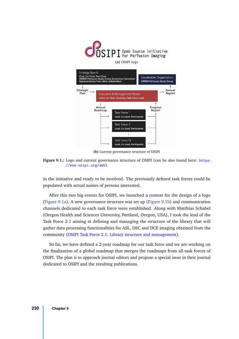
(a) OSIPI logo

(b) Current governance structure of OSIPI

Figure 9.1.: Logo and current governance structure of OSIPI (can be also found here: https:

//www.osipi.org/emb).

in the initiative and ready to be involved. The previously defined task forces could be

populated with actual names of persons interested.

After this two big events for OSIPI, we launched a contest for the design of a logo

(Figure 9.1a). A new governance structure was set up (Figure 9.1b) and communication

channels dedicated to each task force were established. Along with Matthias Schabel

(Oregon Health and Sciences University, Portland, Oregon, USA), I took the lead of the

Task Force 2.1 aiming at defining and managing the structure of the library that will

gather data processing functionalities for ASL, DSC and DCE imaging obtained from the

community (OSIPI Task Force 2.1: Library structure and management).

So far, we have defined a 2-year roadmap for our task force and we are working on

the finalization of a global roadmap that merges the roadmaps from all task forces of

OSIPI. The plan is to approach journal editors and propose a special issue in their journal

dedicated to OSIPI and the resulting publications.

230 Chapter 9

https://www.osipi.org/emb

https://www.osipi.org/emb

https://www.osipi.org/task-force-2-1/

ISMRM White Matter Study Group

The ISMRM White Matter Study Group is the group of members of the International

Society for Magnetic Resonance in Medicine interested in the development and application

of MRI to improve understanding and diagnosis of diseases affecting brain and spinal

cord white matter. ISMRM study groups were created to foster the interactions between

researchers and clinicians interested in common MR topics.

In January 2020, I was nominated to the ballot for the position of Trainee Representa-

tive on the Governing Committee of the White Matter Study Group, and elected to this

position on March 11.

As Trainee Representative of the White Matter Study Group, I am interested in

organizing events to foster the communication and sharing of knowledge across the

community. I would like to bring up the consideration of white matter perfusion in

demyelinating disease. I am also interested in setting up a challenge to elect the most

promising quantitative MRI technique currently available for demyelination assessment

to go to larger clinical trials. Finally, I would like to introduce the consideration of

the benefits and current hurdles of 7T MRI for techniques dedicated to white matter

assessment.

231

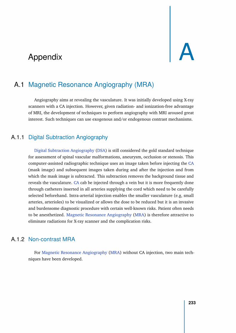
Appendix AA.1 Magnetic Resonance Angiography (MRA)

Angiography aims at revealing the vasculature. It was initially developed using X-ray

scanners with a CA injection. However, given radiation- and ionization-free advantage

of MRI, the development of techniques to perform angiography with MRI aroused great

interest. Such techniques can use exogenous and/or endogenous contrast mechanisms.

A.1.1 Digital Subtraction Angiography

Digital Subtraction Angiography (DSA) is still considered the gold standard technique

for assessment of spinal vascular malformations, aneurysm, occlusion or stenosis. This

computer-assisted radiographic technique uses an image taken before injecting the CA

(mask image) and subsequent images taken during and after the injection and from

which the mask image is subtracted. This subtraction removes the background tissue and

reveals the vasculature. CA cab be injected through a vein but it is more frequently done

through catheters inserted in all arteries supplying the cord which need to be carefully

selected beforehand. Intra-arterial injection enables the smaller vasculature (e.g, small

arteries, arterioles) to be visualized or allows the dose to be reduced but it is an invasive

and burdensome diagnostic procedure with certain well-known risks. Patient often needs

to be anesthetized. Magnetic Resonance Angiography (MRA) is therefore attractive to

eliminate radiations for X-ray scanner and the complication risks.

A.1.2 Non-contrast MRA

For Magnetic Resonance Angiography (MRA) without CA injection, two main tech-

niques have been developed.

233

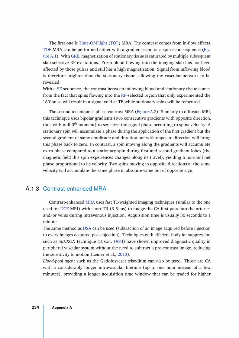
The first one is Time-Of-Flight (TOF) MRA. The contrast comes from in-flow effects.

TOF MRA can be performed either with a gradient-echo or a spin-echo sequence (Fig-

ure A.1). With GRE, magnetization of stationary tissue is saturated by multiple subsequent

slab-selective RF excitations. Fresh blood flowing into the imaging slab has not been

affected by those pulses and still has a high magnetization. Signal from inflowing blood

is therefore brighter than the stationary tissue, allowing the vascular network to be

revealed.

With a SE sequence, the contrast between inflowing blood and stationary tissue comes

from the fact that spins flowing into the RF-selected region that only experimented the

180°pulse will result in a signal void at TE while stationary spins will be refocused.

The second technique is phase-contrast MRA (Figure A.2). Similarly to diffusion MRI,

this technique uses bipolar gradients (two consecutive gradients with opposite direction,

thus with null 0th moment) to sensitize the signal phase according to spins velocity. A

stationary spin will accumulate a phase during the application of the first gradient but the

second gradient of same amplitude and duration but with opposite direction will bring

this phase back to zero. In contrast, a spin moving along the gradients will accumulate

extra-phase compared to a stationary spin during first and second gradient lobes (the

magnetic field this spin experiences changes along its travel), yielding a non-null net

phase proportional to its velocity. Two spins moving in opposite directions at the same

velocity will accumulate the same phase in absolute value but of opposite sign.

A.1.3 Contrast-enhanced MRA

Contrast-enhanced MRA uses fast T1-weighted imaging techniques (similar to the one

used for DCE MRI) with short TR (3-5 ms) to image the CA first pass into the arteries

and/or veins during intravenous injection. Acquisition time is usually 30 seconds to 1

minute.

The same method as DSA can be used (subtraction of an image acquired before injection

to every images acquired post-injection). Techniques with efficient body fat suppression

such as mDIXON technique (Dixon, 1984) have shown improved diagnostic quality in

peripheral vascular system without the need to subtract a pre-contrast image, reducing

the sensitivity to motion (Leiner et al., 2013).

Blood-pool agent such as the Gadofosveset trisodium can also be used. Those are CA

with a considerably longer intravascular lifetime (up to one hour instead of a few

minutes), providing a longer acquisition time window that can be traded for higher

234 Appendix A

(a) TOF MRA with a gradient-echo sequence

(b) TOF MRA with a spin-echo sequence

Figure A.1.: Principle of Time-Of-Flight (TOF) MRA using gradient-echo (a) or spin-echo se-quence (b) (source: radiologycafe.com).

spatial resolution. However, with such CA, both arteries and veins signal is enhanced at

the same time, preventing the distinction between the arterial and venous phases.

The commonly used techniques for contrast-enhanced MRA aim at imaging with a good

temporal resolution to be able to follow the CA uptake (time-resolved MRA) (Grist et al.,

2012). The main strategies are to sample the k-space center more frequently than its

periphery, share data within time frames and temporally interpolate data to fill uncollected

points. Those strategies have been implemented in methods referred as "keyhole" imaging

(Van Vaals et al., 1993) or Block Regional Interpolation Scheme for K-space (BRISK)

(Doyle et al., 1995). With most recent methods such as 3D TRICKS (Time-Resolved

A.1 Magnetic Resonance Angiography (MRA) 235

https://www.radiologycafe.com/radiology-trainees/frcr-physics-notes/mr-angiography

Figure A.2.: Phase-contrast technique (source: mriquestions.com)..

Imaging of Contrast Kinetics) (Korosec et al., 1996), one volume can be acquired every

2-6 second, allowing the spatial frequency uptake of the CA to be updated.

Finally, TOF or phase-contrast techniques can also be applied in conjunction with the CA

injection to exacerbate contrast, either due to reduced T1 and increased inflow effects or

reduced T2* and increased dephasing with flow velocity.

With recent developments of accelerated acquisition techniques (multiple coil arrays,

parallel acquisition approaches, compressed sensing), 3D contrast-enhanced MRA have

now been applied to all vascular territories of the body. One challenge is to trigger the

acquisition when the contrast bolus arrives in the phase of interest in order to distinguish

the arterial and venous phases (Riederer et al., 2018).

A.2 Vascular Occupancy (VASO) MRI

The Vascular Occupancy (VASO) MRI technique was first proposed to remove the

contribution of large vessels to the BOLD signal in functional MRI (Figure A.3). This

technique consists in taking advantage of the different longitudinal relaxation times of

tissues so as to null the signal coming from a specific tissue (here, blood) at the time

of excitation. By applying an inversion RF pulse prior to signal acquisition and with a

well-defined delay (inversion time, TI) calculated based on the tissue T1, the longitudinal

magnetization of the tissue is inverted so that after the delay TI when occurs the 90°RF,

236 Appendix A

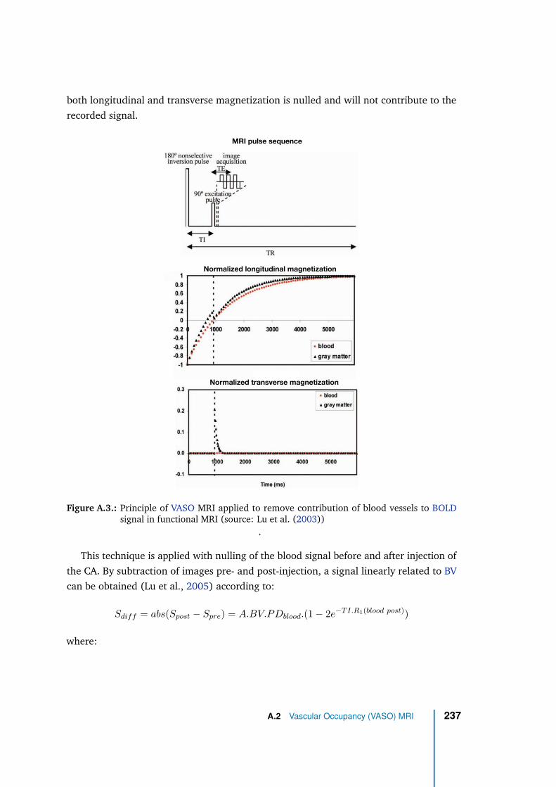
http://mriquestions.com/phase-contrast-mra.html

both longitudinal and transverse magnetization is nulled and will not contribute to the

recorded signal.

MRI pulse sequence

Normalized longitudinal magnetization

Normalized transverse magnetization

Figure A.3.: Principle of VASO MRI applied to remove contribution of blood vessels to BOLDsignal in functional MRI (source: Lu et al. (2003))

.

This technique is applied with nulling of the blood signal before and after injection of

the CA. By subtraction of images pre- and post-injection, a signal linearly related to BV

can be obtained (Lu et al., 2005) according to:

Sdiff = abs(Spost − Spre) = A.BV.PDblood.(1 − 2e−T I.R1(blood post))

where:

A.2 Vascular Occupancy (VASO) MRI 237

• A is the MR signal per mL of water protons at equilibrium; this constant can be

obtained in a CSF-only voxel from an acquisition with long TR and short TE.

• PDblood is the water proton density of blood (0.87).

• TI is the inversion time calculated so as to null blood signal (920 ms at 1.5T, 1088

ms at 3T)

• R1(blood post) is the longitudinal relaxation rate of blood after CA injection:

R1(blood post) = R1(blood) + r1.CCA with CCA the CA concentration in blood

at time of post-injection acquisition.

R1(blood post) can be assumed large enough to consider e−T I.R1(blood post)) ≈ 0 so

that the absolute BV value can be calculated as:

BV =Sdiff

ρbrain.A.Cblood

A normalization by the brain tissue density ρbrain is added to obtain BV in the common unit

of mL/100g tissue. The proof-of-concept study by (Lu et al., 2005) reported respective

values of 5.5 and 1.4 mL/100mL tissue for BV in cortical GM and WM in normal brain

regions within a group of 10 patients with brain tumors at 1.5T (5.6 and 1.5 mL/100mL

tissue at 3T respectively, within 3 multiple sclerosis patients), with a good voxel-wise

correlation between DSC and VASO MRI (R2 = 0.73). The total acquisition time was

6 minutes, including 1 minutes for the DSC acquisition. If values roughly match with

DSC-derived BV values, several confounding factors have nonetheless to be controlled

with this technique (Uh et al., 2009):

(1) The optimal nulling TI can be obtained for one slice only; a slice-wise normalization

by 2e−T Islice.R1(blood) can be added to account for that.

(2) As CA also changes blood T2 and T2*, transverse relaxation effects have been

shown to result in understimation of BV (Uh et al., 2009). Multi-echo acquisition is

recommended to reduce this bias. If not possible, an extrapolation of the signal to

TE=0 can be performed assuming T2 and/or T2* values from literature.

(3) BV estimation might be affected by the CA clearance and post-injection time of the

acquisition. Uh et al. (2009) reported that, in the first 14 minutes after injection, the

CA concentration was high enough to preserve at least 90% of BV effects in the data.

Dependency on post-injection time can be assessed with multiple post-injection

acquisitions with different times.

238 Appendix A

(4) Water exchange between blood and tissue across the blood-brain barrier depends

on the CA concentration and can represent up to 30% of total signal right after

injection but decreases with time. According to Uh et al. (2009), 7 minutes after

injection, water exchange should be reasonably negligible.

(5) CA leakage in tissue because of blood-brain barrier disruption result in an overes-

timation of the BV. Uh et al. (2009) showed that a quadratic extrapolation of the

signal to a post-injection time of zero can considerably reduce this overestimation.

If VASO MRI offers several advantages over DSC (no AIF extraction required, no

restriction related to dynamic acquisitions making signal averaging, regular k-space

sampling or segmented EPI and an increased number of slices possible), it also comes

with disadvantages relative to DSC:

(1) it only estimates BV and does not provide any information about BF, MTT or any

timing information on the bolus,

(2) Contrast (and sensitivity) is intrinsically lower because post-contrast imaging occurs

after bolus peak i.e., when CA concentration has significantly decreased. However,

averages can help balance this disadvantage by reducing noise and consequently

increasing CNR.

A.3 Grading tools to quantify patients’ neurological status

in Degenerative Cervical Myelopathy

A.3.1 Nurick’s grading system (Nurick, 1972)

0: Signs or symptoms of root involvement but without evidence of spinal cord disease

1: Signs of spinal cord disease but no difficulty in walking

2: Slight difficulty in walking which did not prevent full-time employment

3: Difficulty in walking which prevented full-time employment or the ability to do all

housework, but which was not so severe as to require someone else’s help to walk

4: Able to walk only with someone else’s help or with the aid of a frame

A.3 Grading tools to quantify patients’ neurological status in Degenerative

Cervical Myelopathy

239

5: Chair bound or bedridden

A.3.2 Modified Japanese Orthopedic Association Scale (mJOA)

This is the version from Chiles et al. (1999) but slightly differing version was also

proposed by Benzel et al. (1991).

A) Motor dysfunction of the upper extremity

0: Unable to feed oneself

1: Unable to used knife and fork; able to eat with a spoon

2: Able to use knife and fork with much difficulty

3: Able to use knife and fork with slight difficulty

4: None

B) Motor dysfunction of the lower extremity

0: Unable to walk

1: Can walk on flat floor with walking aid

2: Can walk up and/or down stairs with handrail

3: Lack of stability and smooth gait

4: None

C) Sensory deficit for upper extremity

0: Severe sensory loss or pain

1: Mild sensory loss

2: None

D) Sensory deficit for lower extremity



240 Appendix A

2: None

E) Sensory deficit for trunk



2: None

F) Sphincter dysfunction

0: Unable to void

1: Marked difficulty in micturition (retention)

2: Difficulty in micturition (frequency, hesitation)

3: None

The sum of each number gives the mJOA score, the highest score being 17/17.

A.4 Conception of a perfusion phantom

Imaging perfusion is imaging a moving fluid within small compartments. However,

common phantoms are only made of static components. Very few flow phantoms are

commercially available, and the available phantoms are very expensive (∼25,000C, e.g.

Shelley Medical Imaging Technologies Multi-modality DCE Perfusion Flow Phantom).

Nevertheless, phantoms are extremely helpful to optimize and test acquisition protocols

and particular effects of parameters. In this view, a perfusion phantom was built based

on a dyalizer (Fresenius Medical Care, model FX100), a pump and long tubes to keep the

pump outside the magnet room (Figure A.4a). A dyalizer is an artificial filter for blood

made of synthetic fibers and dedicted to replicate the kidneys function, i.e. removing

waste materials, toxins, excess salt and fluids from the body. The fibers are hollow with

microscopic pores, making an artificial semi-permeable membrane. It is used for in case

of kidney failure: a special dialysis-fluid flows in the outside of the fibers while blood

flows through the fibers. The toxins, urea and other small particles then pass through the

semi-permeable membrane and are eliminated, meaning that water also goes through

this membrane.

A.4 Conception of a perfusion phantom 241

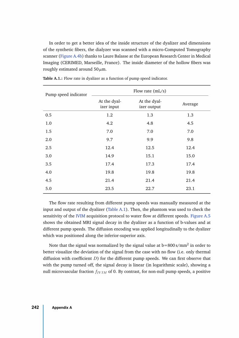
http://www.simutec.com/Docs/DCE%20Perfusion%20Flow%20Phantom%20for%20CT%20MRI%20&%20PET%20Flyer%20HR.pdf

In order to get a better idea of the inside structure of the dyalizer and dimensions

of the synthetic fibers, the dialyzer was scanned with a micro-Computed Tomography

scanner (Figure A.4b) thanks to Laure Balasse at the European Research Center in Medical

Imaging (CERIMED, Marseille, France). The inside diameter of the hollow fibers was

roughly estimated around 50 µm.

Table A.1.: Flow rate in dyalizer as a function of pump speed indicator.

Pump speed indicatorFlow rate (mL/s)

At the dyal-izer input

At the dyal-izer output

Average

0.5 1.2 1.3 1.3

1.0 4.2 4.8 4.5

1.5 7.0 7.0 7.0

2.0 9.7 9.9 9.8

2.5 12.4 12.5 12.4

3.0 14.9 15.1 15.0

3.5 17.4 17.3 17.4

4.0 19.8 19.8 19.8

4.5 21.4 21.4 21.4

5.0 23.5 22.7 23.1

The flow rate resulting from different pump speeds was manually measured at the

input and output of the dyalizer (Table A.1). Then, the phantom was used to check the

sensitivity of the IVIM acquisition protocol to water flow at different speeds. Figure A.5

shows the obtained MRI signal decay in the dyalizer as a function of b-values and at

different pump speeds. The diffusion encoding was applied longitudinally to the dyalizer

which was positioned along the inferior-superior axis.

Note that the signal was normalized by the signal value at b=800 s/mm2 in order to

better visualize the deviation of the signal from the case with no flow (i.e. only thermal

diffusion with coefficient D) for the different pump speeds. We can first observe that

with the pump turned off, the signal decay is linear (in logarithmic scale), showing a

null microvascular fraction fIV IM of 0. By contrast, for non-null pump speeds, a positive

242 Appendix A

fIV IM is measured and the decay at low b-values gets faster (the pseudo-diffusion

coefficient D∗ increases). Secondly, it is interesting to notice that even at high b-values

(600 and even 700 s/mm2), the flow rate has an effect on the signal as evidenced by the

difference in the linear fit (based on high b-values only) across pump speeds.

To have a rough idea of the flow rate provided by the pump compare to in-vivo flow

rates, let us consider, on the one hand, a value of 60 mL/100g tissue/min in the healthy

gray matter. Given a gray matter density of 1.04 g/cm3, this corresponds to a blood flow of

58.0 mL/100cm3/min. On the other hand, the priming volume of the dyalizer is 116cm3

(according to the vendor). Therefore, a flow rate of 4.5 mL/s (pump speed indicator on

1) would correspond to a flow of 232.8 mL/100cm3/min inside the dyalizer. This is about

4 times higher than the gray matter blood flow, and still, we see flow effects on the high

b-values. This result supports that the one-step fit is more appropriate in case of low

perfusion levels. It also suggests that considering higher b-values (≥800 s/mm2), which

is possible thanks to the increased SNR at 7T, might improve the separation between

perfusion and pure diffusion effects in the phantom.


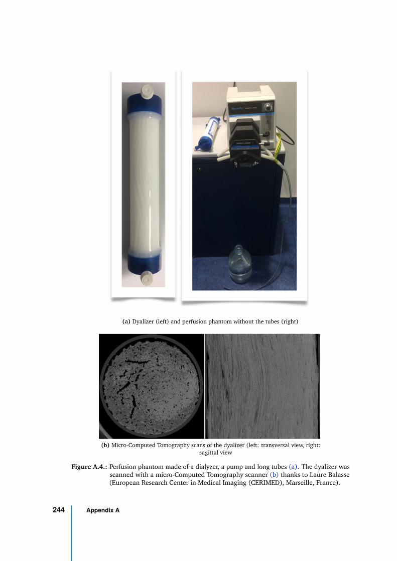
(a) Dyalizer (left) and perfusion phantom without the tubes (right)

(b) Micro-Computed Tomography scans of the dyalizer (left: transversal view, right:sagittal view

Figure A.4.: Perfusion phantom made of a dialyzer, a pump and long tubes (a). The dyalizer wasscanned with a micro-Computed Tomography scanner (b) thanks to Laure Balasse(European Research Center in Medical Imaging (CERIMED), Marseille, France).

244 Appendix A

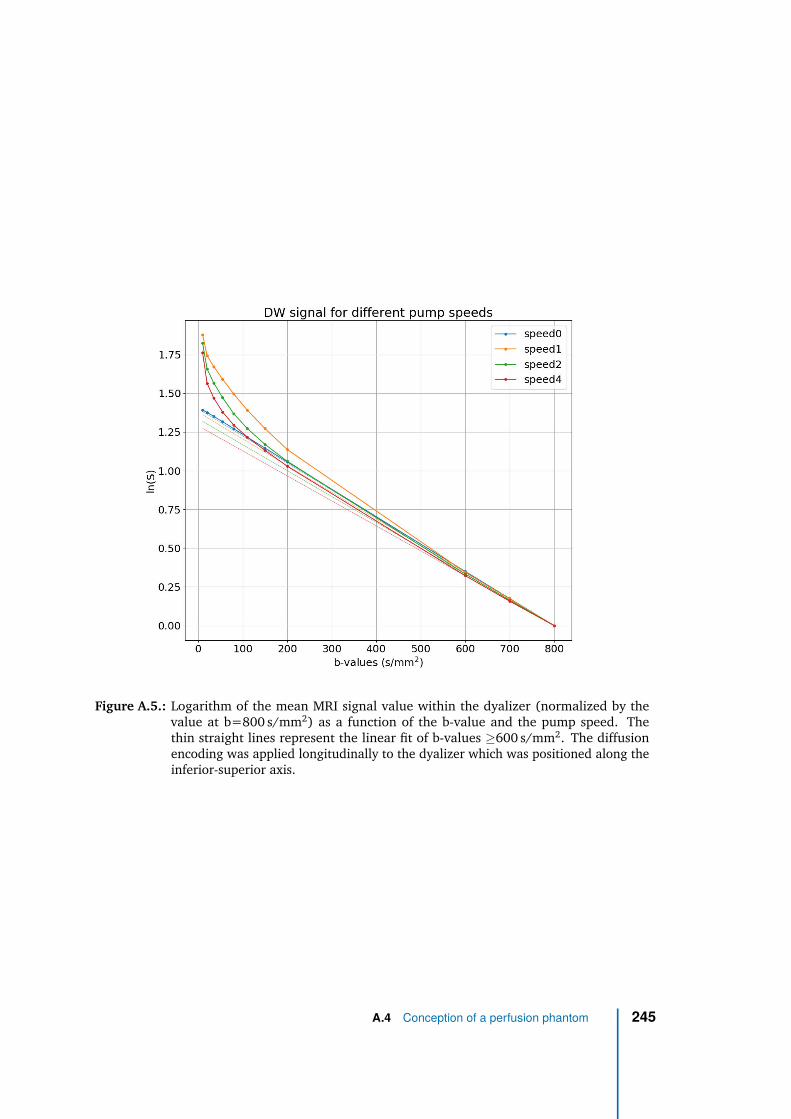
Figure A.5.: Logarithm of the mean MRI signal value within the dyalizer (normalized by thevalue at b=800 s/mm2) as a function of the b-value and the pump speed. Thethin straight lines represent the linear fit of b-values ≥600 s/mm2. The diffusionencoding was applied longitudinally to the dyalizer which was positioned along theinferior-superior axis.


Bibliography

Ahlgren, André, Linda Knutsson, Ronnie Wirestam, et al. (May 2016). “Quantification of mi-crocirculatory parameters by joint analysis of flow-compensated and non-flow-compensatedintravoxel incoherent motion (IVIM) data: Joint Analysis of Flow-Compensated and Non-Flow-Compensated IVIM Data”. en. In: NMR in Biomedicine 29.5, pp. 640–649. DOI: 10.1002/nbm.

3505 (cit. on p. 78).

Ahn, C. B., J. H. Kim, and Z. H. Cho (Mar. 1986). “High-Speed Spiral-Scan Echo Planar NMRImaging-I”. In: IEEE Transactions on Medical Imaging 5.1, pp. 2–7. DOI: 10.1109/TMI.1986.

4307732 (cit. on pp. 35, 36).

Al-Mefty, Ossama, H. Louis Harkey, Isam Marawi, et al. (Oct. 1993). “Experimental chroniccompressive cervical myelopathy”. en. In: Journal of Neurosurgery 79.4, pp. 550–561. DOI:10.3171/jns.1993.79.4.0550 (cit. on p. 87).

Alshareef, Mohammed, Vibhor Krishna, Jahid Ferdous, et al. (Sept. 2014). “Effect of Spinal CordCompression on Local Vascular Blood Flow and Perfusion Capacity”. en. In: PLoS ONE 9.9.Ed. by Michael Fehlings, e108820. DOI: 10.1371/journal.pone.0108820 (cit. on pp. 112, 113,217, 219).

Alsop, David C., John A. Detre, Xavier Golay, et al. (Jan. 2015). “Recommended implementationof arterial spin-labeled perfusion MRI for clinical applications: A consensus of the ISMRMperfusion study group and the European consortium for ASL in dementia: RecommendedImplementation of ASL for Clinical Applications”. en. In: Magnetic Resonance in Medicine 73.1,pp. 102–116. DOI: 10.1002/mrm.25197 (cit. on pp. 69–73, 211).

Amato, Alexandre Campos Moraes and Noedir Antônio Groppo Stolf (Sept. 2015). “Anatomia dacirculação medular”. en. In: Jornal Vascular Brasileiro 14.3, pp. 248–252. DOI: 10.1590/1677-

5449.0004 (cit. on pp. 16, 19).

Andersson, Jesper L. R., Stefan Skare, and John Ashburner (Oct. 2003). “How to correct suscepti-bility distortions in spin-echo echo-planar images: application to diffusion tensor imaging”. In:NeuroImage 20.2, pp. 870–888. DOI: 10.1016/S1053-8119(03)00336-7 (cit. on p. 34).

Apruzzese, Alessio, Mauro Silvestrini, Roberto Floris, et al. (2001). “Cerebral Hemodynamicsin Asymptomatic Patients with Internal Carotid Artery Occlusion: A Dynamic SusceptibilityContrast MR and Transcranial Doppler Study”. en. In: p. 6 (cit. on p. 66).

247



https://doi.org/10.1109/TMI.1986.4307732

https://doi.org/10.1109/TMI.1986.4307732

https://doi.org/10.3171/jns.1993.79.4.0550



https://doi.org/10.1590/1677-5449.0004

https://doi.org/10.1590/1677-5449.0004

https://doi.org/10.1016/S1053-8119(03)00336-7

Atkinson, Ian C., Laura Renteria, Holly Burd, Neil H. Pliskin, and Keith R. Thulborn (Nov. 2007).“Safety of human MRI at static fields above the FDA 8T guideline: Sodium imaging at 9.4T doesnot affect vital signs or cognitive ability”. en. In: Journal of Magnetic Resonance Imaging 26.5,pp. 1222–1227. DOI: 10.1002/jmri.21150 (cit. on p. 49).

Baba, Hisatoshi, Yasuhisa Maezawa, Shinichi Imura, et al. (Feb. 1996). “Quantitative analysis ofthe spinal cord motoneuron under chronic compression: an experimental observation in themouse”. en. In: Journal of Neurology 243.2, pp. 109–116. DOI: 10.1007/BF02443999 (cit. onpp. 105, 212, 213).

Baba, Hisatoshi, Yasuhisa Maezawa, Kenzo Uchida, et al. (Apr. 1997). “Three-dimensional to-pographic analysis of spinal accessory motoneurons under chronic mechanical compression:an experimental study in the mouse”. en. In: Journal of Neurology 244.4, pp. 222–229. DOI:10.1007/s004150050076 (cit. on pp. 105, 212, 213).

Bailly, Nicolas, Lucien Diotalevi, Marie-Hélène Beauséjour, et al. (Apr. 2020). “Numerical in-vestigation of the relative effect of disc bulging and ligamentum flavum hypertrophy onthe mechanism of central cord syndrome”. en. In: Clinical Biomechanics 74, pp. 58–65. DOI:10.1016/j.clinbiomech.2020.02.008 (cit. on p. 115).

Barker, Anthony T, Reza Jalinous, and Ian L Freeston (1985). “Non-invasive magnetic stimulationof human motor cortex”. In: The Lancet 325.8437. Publisher: Elsevier, pp. 1106–1107 (cit. onp. 97).

Baron, Eli M. and William F. Young (Jan. 2007). “Cervical Spondylotic Myelopathy: A briefreview of its pathophysiology, clinical course, and diagnosis”. en. In: Neurosurgery 60.suppl_1,S1–35–S1–41. DOI: 10.1227/01.NEU.0000215383.64386.82 (cit. on p. 90).

Barry, Robert L., Baxter P. Rogers, Benjamin N. Conrad, Seth A. Smith, and John C. Gore (June2016). “Reproducibility of resting state spinal cord networks in healthy volunteers at 7 Tesla”.en. In: NeuroImage 133, pp. 31–40. DOI: 10.1016/j.neuroimage.2016.02.058 (cit. on pp. 52,54).

Barry, Robert L, Seth A Smith, Adrienne N Dula, and John C Gore (Aug. 2014). “Resting statefunctional connectivity in the human spinal cord”. en. In: eLife 3, e02812. DOI: 10.7554/eLife.

02812 (cit. on p. 52).

Barry, Robert L., S. Johanna Vannesjo, Samantha By, John C. Gore, and Seth A. Smith (Mar. 2018).“Spinal cord MRI at 7T”. en. In: NeuroImage 168, pp. 437–451. DOI: 10.1016/j.neuroimage.

2017.07.003 (cit. on pp. 38, 46, 50).

Basser, P. J., J. Mattiello, and D. Lebihan (Mar. 1994). “Estimation of the Effective Self-DiffusionTensor from the NMR Spin Echo”. In: Journal of Magnetic Resonance, Series B 103.3, pp. 247–254. DOI: 10.1006/jmrb.1994.1037 (cit. on p. 75).

Baucher, Guillaume (2019). “Cartographie T1 de la moelle spinale cervicale dans l’évaluationdes patients atteints de myélopathie cervicale dégénérative”. French. Research master inneurosciences. Marseille: Aix-Marseille University (cit. on p. 93).

248 Bibliography


https://doi.org/10.1007/BF02443999

https://doi.org/10.1007/s004150050076


https://doi.org/10.1227/01.NEU.0000215383.64386.82


https://doi.org/10.7554/eLife.02812

https://doi.org/10.7554/eLife.02812



https://doi.org/10.1006/jmrb.1994.1037

Beauséjour, Marie-Hélène, Yvan Petit, Jeremy Hagen, et al. (May 2020). “Contribution of injuredposterior ligamentous complex and intervertebral disc on post-traumatic instability at thecervical spine”. en. In: Computer Methods in Biomechanics and Biomedical Engineering, pp. 1–12.DOI: 10.1080/10255842.2020.1767776 (cit. on p. 115).

Benzel, EC, J Lancon, L Kesterson, and T Hadden (Sept. 1991). “Cervical laminectomy and dentateligament section for cervical spondylotic myelopathy”. eng. In: Journal of spinal disorders 4.3,pp. 286–295. DOI: 10.1097/00002517-199109000-00005 (cit. on pp. 93, 240).

Berge, Jérôme, Bertrand Marque, Jean-Marc Vital, Jacques Sénégas, and Jean-Marie Caillé (July1999). “Age-Related Changes in the Cervical Spines of Front-Line Rugby Players”. en. In: TheAmerican Journal of Sports Medicine 27.4, pp. 422–429. DOI: 10.1177/03635465990270040401

(cit. on p. 87).

Bergström, Jörgen (2015). “Continuum Mechanics Foundations”. en. In: Mechanics of SolidPolymers. Elsevier, pp. 131–207. DOI: 10.1016/B978- 0- 323- 31150- 2.00004- 2 (cit. onp. 102).

Bertleff, Marco, Sebastian Domsch, Sebastian Weingärtner, et al. (Dec. 2017). “Diffusion parametermapping with the combined intravoxel incoherent motion and kurtosis model using artificialneural networks at 3 T”. en. In: NMR in Biomedicine 30.12, e3833. DOI: 10.1002/nbm.3833

(cit. on p. 78).

Betts, J Gordon, Peter Desaix, Eddie Johnson, et al. (2018). Anatomy & Physiology. en (cit. onp. 107).

Bianciardi, Marta, Jonathan R. Polimeni, Kawin Setsompop, et al. (2014). “Evaluation of dynamicoff-resonance correction of respiratory instability in MRI signals for high-order sphericalharmonic basis set and multivariate modeling of respiratory sources”. In: Proc. Int. Soc. Magn.Reson. Med. 22. Milan, Italy, p. 1623 (cit. on p. 205).

Bihan, Denis Le (Nov. 1995). “Molecular diffusion, tissue microdynamics and microstructure”. en.In: NMR in Biomedicine 8.7, pp. 375–386. DOI: 10.1002/nbm.1940080711 (cit. on p. 75).

Bilston, Lynne E (2011). Neural tissue biomechanics. Vol. 3. Springer Science & Business Media(cit. on p. 104).

Bilston, Lynne E. and Lawrence E. Thibault (Sept. 1995). “The mechanical properties of thehuman cervical spinal cordIn Vitro”. en. In: Annals of Biomedical Engineering 24.S1, pp. 67–74.DOI: 10.1007/BF02770996 (cit. on p. 104).

Bisdas, Sotirios and Uwe Klose (Aug. 2015). “IVIM analysis of brain tumors: an investigation ofthe relaxation effects of CSF, blood, and tumor tissue on the estimated perfusion fraction”.en. In: Magnetic Resonance Materials in Physics, Biology and Medicine 28.4, pp. 377–383. DOI:10.1007/s10334-014-0474-z (cit. on p. 78).

Bisdas, Sotirios, Tong San Koh, Constantin Roder, et al. (Oct. 2013). “Intravoxel incoherent motiondiffusion-weighted MR imaging of gliomas: feasibility of the method and initial results”. en. In:Neuroradiology 55.10, pp. 1189–1196. DOI: 10.1007/s00234-013-1229-7 (cit. on p. 78).

Bibliography 249

https://doi.org/10.1080/10255842.2020.1767776

https://doi.org/10.1097/00002517-199109000-00005

https://doi.org/10.1177/03635465990270040401

https://doi.org/10.1016/B978-0-323-31150-2.00004-2


https://doi.org/10.1002/nbm.1940080711

https://doi.org/10.1007/BF02770996

https://doi.org/10.1007/s10334-014-0474-z

https://doi.org/10.1007/s00234-013-1229-7

Bloch, Felix (1946). “Nuclear Induction”. In: Physical Review 70, pp. 460–474 (cit. on p. 24).

Block, F, WW Hansen, and M Packard (1946). “The nuclear induction experiment”. In: PhysicalReview 70.7-8, pp. 474–485 (cit. on p. 24).

Bloembergen, N., E. M. Purcell, and R. V. Pound (Apr. 1948). “Relaxation Effects in NuclearMagnetic Resonance Absorption”. In: Physical Review 73.7. Publisher: American Physical Society,pp. 679–712. DOI: 10.1103/PhysRev.73.679 (cit. on p. 42).

Boer, Vincent O., Bart L. vd Bank, Gerard van Vliet, Peter R. Luijten, and Dennis W. J. Klomp (Feb.2012). “Direct B0 field monitoring and real-time B0 field updating in the human breast at 7tesla”. en. In: Magnetic Resonance in Medicine 67.2, pp. 586–591. DOI: 10.1002/mrm.23272

(cit. on p. 205).

Bowen, Brian C, Steven DePrima, Pradip M Pattany, et al. (1996). “MR Angiography of NormalIntradural Vessels of the Thoracolumbar Spine”. en. In: p. 12 (cit. on p. 83).

Brand, Michael, Stephan Ellmann, Matthias Sommer, et al. (Nov. 2015). “Influence of Cardiac MRImaging on DNA Double-Strand Breaks in Human Blood Lymphocytes”. en. In: Radiology 277.2,pp. 406–412. DOI: 10.1148/radiol.2015150555 (cit. on p. 50).

Breig, Alf, Ian Turnbull, and Ove Hassler (1966). “Effects of mechanical stresses on the spinalcord in cervical spondylosis: a study on fresh cadaver material”. In: Journal of neurosurgery25.1, pp. 45–56 (cit. on pp. 87, 90).

Bulte, Daniel, Peter Chiarelli, Richard Wise, and Peter Jezzard (Oct. 2007). “Measurement ofcerebral blood volume in humans using hyperoxic MRI contrast”. en. In: Journal of MagneticResonance Imaging 26.4, pp. 894–899. DOI: 10.1002/jmri.21096 (cit. on p. 68).

Burrows, Edmund H. (1963). “The sagittal diameter of the spinal canal in cervical spondylosis”. In:Clinical Radiology 14.1, pp. 77 –86. DOI: https://doi.org/10.1016/S0009-9260(63)80015-X

(cit. on p. 216).

Buxton, Richard B., Lawrence R. Frank, Eric C. Wong, et al. (Sept. 1998). “A general kinetic modelfor quantitative perfusion imaging with arterial spin labeling”. en. In: Magnetic Resonance inMedicine 40.3, pp. 383–396. DOI: 10.1002/mrm.1910400308 (cit. on p. 71).

Cadotte, D. W., A. Cadotte, J. Cohen-Adad, et al. (Apr. 2015). “Characterizing the Locationof Spinal and Vertebral Levels in the Human Cervical Spinal Cord”. In: American Journal ofNeuroradiology 36, pp. 803–810. DOI: 10.3174/ajnr.A4192 (cit. on p. 11).

Calamante, Fernando (2013). “Arterial input function in perfusion MRI: A comprehensive review”.en. In: Progress in Nuclear Magnetic Resonance Spectroscopy, p. 32 (cit. on pp. 61, 63).

Calamante, Fernando, David L. Thomas, Gaby S. Pell, Jonna Wiersma, and Robert Turner (July1999). “Measuring Cerebral Blood Flow Using Magnetic Resonance Imaging Techniques”. en.In: Journal of Cerebral Blood Flow & Metabolism 19.7, pp. 701–735. DOI: 10.1097/00004647-

199907000-00001 (cit. on p. 62).

250 Bibliography

https://doi.org/10.1103/PhysRev.73.679


https://doi.org/10.1148/radiol.2015150555



https://doi.org/10.1002/mrm.1910400308


https://doi.org/10.1097/00004647-199907000-00001

https://doi.org/10.1097/00004647-199907000-00001

Callot, V, G Duhamel, P Moulin, and P J Cozzone (2011). “Intra Voxel Incoherent Motion (IVIM)MRI of the human spinal cord: preliminary results and potentiality”. en. In: Proc. Intl. Soc. Mag.Reson. Med. 19, p. 1 (cit. on p. 80).

Callot, Virginie, Guillaume Duhamel, Jérôme Laurin, André Mauès de Paula, and Patrick J Cozzone(2012). “Intra Voxel Incoherent Motion (IVIM) MRI: an alternative method to get spinal cord(SC) vascular description. Preliminary results in healthy and injured mice.” en. In: Proc. Intl.Soc. Mag. Reson. Med. 20, p. 1037 (cit. on pp. 80, 210, 211).

Carlson, Gregory D, Carey D Gorden, Shigenobu Nakazowa, et al. (2000). “Perfusion-limitedrecovery of evoked potential function after spinal cord injury”. In: Spine 25.10, pp. 1218–1226(cit. on pp. 110, 112).

Carlson, Gregory D, Karen E Warden, James M Barbeau, et al. (1997). “Viscoelastic relaxationand regional blood flow response to spinal cord compression and decompression”. In: Spine22.12, pp. 1285–1291 (cit. on pp. 110, 112).

Chiles III, Bennie W., Michael A. Leonard, Haroon F. Choudhri, and Paul R. Cooper (Apr. 1999).“Cervical Spondylotic Myelopathy: Patterns of Neurological Deficit and Recovery after AnteriorCervical Decompression”. In: Neurosurgery 44.4, pp. 762–769. DOI: 10 . 1097 / 00006123 -

199904000-00041 (cit. on pp. 93, 240).

Chomiak, J., J. Dvorak, J. Antinnes, and A. Sandler (June 1995). “Motor evoked potentials:appropriate positioning of recording electrodes for diagnosis of spinal disorders”. en. In:European Spine Journal 4.3, pp. 180–185. DOI: 10.1007/BF00298243 (cit. on p. 97).

Christensen, Søren, Kim Mouridsen, Ona Wu, et al. (June 2009). “Comparison of 10 PerfusionMRI Parameters in 97 Sub-6-Hour Stroke Patients Using Voxel-Based Receiver OperatingCharacteristics Analysis”. en. In: Stroke 40.6, pp. 2055–2061. DOI: 10.1161/STROKEAHA.108.

546069 (cit. on p. 62).

Cohen-Adad, J. and C. Wheeler-Kingshott (2014). Quantitative MRI of the Spinal Cord. ElsevierScience (cit. on p. 38).

Collins, Christopher M. and Zhangwei Wang (May 2011). “Calculation of radiofrequency elec-tromagnetic fields and their effects in MRI of human subjects: RF Field Calculations in MRI”.en. In: Magnetic Resonance in Medicine 65.5, pp. 1470–1482. DOI: 10.1002/mrm.22845 (cit. onp. 48).

Cowling, Tara and Nina Frey (2019). “Macrocyclic and Linear Gadolinium Based Contrast Agentsfor Adults Undergoing Magnetic Resonance Imaging: A Review of Safety”. In: Canadian Agencyfor Drugs and Technologies in Health (cit. on pp. 196, 197).

Czyz, Marcin, Krzysztof Scigala, Wlodzimierz Jarmundowicz, and Romuald Bedzinski (2011).“Numerical model of the human cervical spinal cord-the development and validation.” In: Actaof Bioengineering & Biomechanics 13.4 (cit. on p. 109).

Bibliography 251

https://doi.org/10.1097/00006123-199904000-00041

https://doi.org/10.1097/00006123-199904000-00041

https://doi.org/10.1007/BF00298243

https://doi.org/10.1161/STROKEAHA.108.546069



De Leener, Benjamin, Vladimir S. Fonov, D. Louis Collins, et al. (2018). “PAM50: Unbiasedmultimodal template of the brainstem and spinal cord aligned with the ICBM152 space”. In:NeuroImage 165, pp. 170 –179. DOI: 10.1016/j.neuroimage.2017.10.041 (cit. on p. 13).

Dietrich, Benjamin E., David O. Brunner, Bertram J. Wilm, et al. (Apr. 2016). “A field camera forMR sequence monitoring and system analysis: MR Sequence Monitoring and System AnalysisCamera”. en. In: Magnetic Resonance in Medicine 75.4, pp. 1831–1840. DOI: 10.1002/mrm.25770

(cit. on p. 36).

Dixon, W T (Oct. 1984). “Simple proton spectroscopic imaging.” In: Radiology 153.1. Publisher:Radiological Society of North America, pp. 189–194. DOI: 10.1148/radiology.153.1.6089263

(cit. on p. 234).

Donahue, Kathleen M, Hendrikus GJ Krouwer, Scott D Rand, et al. (2000). “Utility of simultane-ously acquired gradient-echo and spin-echo cerebral blood volume and morphology maps inbrain tumor patients”. In: Magnetic resonance in medicine 43.6. Publisher: Wiley Online Library,pp. 845–853 (cit. on p. 64).

Doppman, John L (1975). “The mechanism of ischemia in anteroposterior compression of thespinal cord.” In: Investigative radiology 10.6, pp. 543–551 (cit. on pp. 117, 217).

Dortch, Richard D., Adrienne N. Dula, K. Li, et al. (2012). “Quantitative magnetization transferimaging of human cervical spinal cord at 7 Tesla”. In: Proc. Int. Soc. Magn. Reson. Med. 20.Melbourne, Victoria, Australia, p. 0614 (cit. on p. 52).

Doyle, Mark, Edward G. Walsh, Gerald G. Blackwell, and Gerald M. Pohost (Feb. 1995). “BlockRegional Interpolation Scheme for k-Space (BRISK): A Rapid Cardiac Imaging Technique”. en.In: Magnetic Resonance in Medicine 33.2, pp. 163–170. DOI: 10.1002/mrm.1910330204 (cit. onp. 235).

Duerst, Yolanda, Bertram J. Wilm, Michael Wyss, et al. (Aug. 2016). “Utility of real-time fieldcontrol in T 2 *-Weighted head MRI at 7T: Utility of Real-Time Field Control”. en. In: MagneticResonance in Medicine 76.2, pp. 430–439. DOI: 10.1002/mrm.25838 (cit. on p. 45).

Duggal, N., D. Rabin, R. Bartha, et al. (Mar. 2010). “Brain reorganization in patients withspinal cord compression evaluated using fMRI”. en. In: Neurology 74.13, pp. 1048–1054. DOI:10.1212/WNL.0b013e3181d6b0ea (cit. on p. 98).

Duhamel, Guillaume, Virginie Callot, Patrick J. Cozzone, and Frank Kober (2008). “Spinal cordblood flow measurement by arterial spin labeling”. In: Magnetic Resonance in Medicine 59,pp. 846–854. DOI: 10.1002/mrm.21567 (cit. on pp. 7, 79, 80).

Duhamel, Guillaume, Virginie Callot, Patrick Decherchi, et al. (2009). “Mouse lumbar and cervicalspinal cord blood flow measurements by arterial spin labeling: Sensitivity optimization and firstapplication”. In: Magnetic Resonance in Medicine 62, pp. 430–439. DOI: 10.1002/mrm.22015

(cit. on pp. 7, 79).

252 Bibliography




https://doi.org/10.1002/mrm.1910330204


https://doi.org/10.1212/WNL.0b013e3181d6b0ea



Dula, Adrienne N., Siddharama Pawate, Lindsey M. Dethrage, et al. (Sept. 2016). “Chemicalexchange saturation transfer of the cervical spinal cord at 7 T: Cest of the Cervical Spinal CordAT 7 T”. en. In: NMR in Biomedicine 29.9, pp. 1249–1257. DOI: 10.1002/nbm.3581 (cit. onp. 53).

Dvorak, Jiri, Martin Sutter, and Joerg Herdmann (2005). “Cervical myelopathy: clinical andneurophysiological evaluation”. In: The Aging Spine. Ed. by Max Aebi, Robert Gunzburg, andMarek Szpalski. Berlin, Heidelberg: Springer Berlin Heidelberg, pp. 99–105 (cit. on p. 96).

Edwards, WC and H LaRocca (1983). “The developmental segmental sagittal diameter of thecervical spinal canal in patients with cervical spondylosis”. eng. In: Spine 8.1, pp. 20–27 (cit. onp. 90).

El-Rich, Marwan, Pierre-Jean Arnoux, Eric Wagnac, Christian Brunet, and Carl-Eric Aubin (June2009). “Finite element investigation of the loading rate effect on the spinal load-sharingchanges under impact conditions”. In: Journal of Biomechanics 42.9, pp. 1252–1262. DOI:10.1016/j.jbiomech.2009.03.036 (cit. on pp. 114, 116).

Ellingson, Benjamin M., Noriko Salamon, Anthony J. Hardy, and Langston T. Holly (Oct. 2015).“Prediction of Neurological Impairment in Cervical Spondylotic Myelopathy using a Combinationof Diffusion MRI and Proton MR Spectroscopy”. en. In: PLOS ONE 10.10. Ed. by MohammedShamji, e0139451. DOI: 10.1371/journal.pone.0139451 (cit. on p. 97).

Ellingson, Benjamin M., Davis C. Woodworth, Kevin Leu, Noriko Salamon, and Langston T. Holly(Aug. 2019). “Spinal Cord Perfusion MR Imaging Implicates Both Ischemia and Hypoxia inthe Pathogenesis of Cervical Spondylosis”. en. In: World Neurosurgery 128, e773–e781. DOI:10.1016/j.wneu.2019.04.253 (cit. on p. 81).

European Parliament and Council (2013). “Directive 2013/35/EU of 26 June 2013 on theminimum health and safety requirements regarding the exposure of workers to the risks arisingfrom physical agents (electromagnetic fields)”. In: L 179/1.EU (Ed.) Pp. 1–21 (cit. on p. 50).

Federau, C., S. Sumer, F. Becce, et al. (Aug. 2014). “Intravoxel incoherent motion perfusionimaging in acute stroke: initial clinical experience”. en. In: Neuroradiology 56.8, pp. 629–635.DOI: 10.1007/s00234-014-1370-y (cit. on p. 79).

Federau, Christian, Patric Hagmann, Philippe Maeder, et al. (Aug. 2013). “Dependence of BrainIntravoxel Incoherent Motion Perfusion Parameters on the Cardiac Cycle”. en. In: PLOS ONE8.8. Ed. by Jeroen Hendrikse, e72856. DOI: 10.1371/journal.pone.0072856 (cit. on pp. 77,200).

Federau, Christian, Kieran O’Brien, Adrien Birbaumer, et al. (Feb. 2015). “Functional Mappingof the Human Visual Cortex with Intravoxel Incoherent Motion MRI”. en. In: PLOS ONE 10.2,e0117706. DOI: 10.1371/journal.pone.0117706 (cit. on p. 78).

Fehlings, M. G. and G. Skaf (Dec. 1998). “A review of the pathophysiology of cervical spondyloticmyelopathy with insights for potential novel mechanisms drawn from traumatic spinal cordinjury”. eng. In: Spine 23.24, pp. 2730–2737 (cit. on pp. 90, 213, 214).

Bibliography 253





https://doi.org/10.1007/s00234-014-1370-y



Fehlings, Michael G., Lindsay A. Tetreault, K. Daniel Riew, et al. (Sept. 2017). “A Clinical PracticeGuideline for the Management of Patients With Degenerative Cervical Myelopathy: Recommen-dations for Patients With Mild, Moderate, and Severe Disease and Nonmyelopathic PatientsWith Evidence of Cord Compression”. en. In: Global Spine Journal 7.3_suppl, 70S–83S. DOI:10.1177/2192568217701914 (cit. on p. 94).

Fehlings, Michael G., Jefferson R. Wilson, Spyridon K. Karadimas, Paul M. Arnold, and BrankoKopjar (Oct. 2013). “Clinical Evaluation of a Neuroprotective Drug in Patients With CervicalSpondylotic Myelopathy Undergoing Surgical Treatment: Design and Rationale for the CSM-Protect Trial”. en. In: Spine 38, S68–S75. DOI: 10.1097/BRS.0b013e3182a7e9b0 (cit. onp. 94).

Feinberg, David A. and Koichi Oshio (1991). “GRASE (gradient-and spin-echo) MR imaging: anew fast clinical imaging technique”. In: Radiology 181, pp. 597–602 (cit. on p. 73).

Fiford, Rodney J. and Lynne E. Bilston (July 2005). “The mechanical properties of rat spinal cordin vitro”. en. In: Journal of Biomechanics 38.7, pp. 1509–1515. DOI: 10.1016/j.jbiomech.

2004.07.009 (cit. on p. 104).

Figley, C.R. and P.W. Stroman (July 2007). “Investigation of human cervical and upper thoracicspinal cord motion: Implications for imaging spinal cord structure and function”. en. In:Magnetic Resonance in Medicine 58.1, pp. 185–189. DOI: 10.1002/mrm.21260 (cit. on p. 200).

Figley, C.R., D. Yau, and P.W. Stroman (Sept. 2008). “Attenuation of Lower-Thoracic, Lumbar,and Sacral Spinal Cord Motion: Implications for Imaging Human Spinal Cord Structure andFunction”. en. In: American Journal of Neuroradiology 29.8, pp. 1450–1454. DOI: 10.3174/

ajnr.A1154 (cit. on p. 200).

Finkenstaedt, Tim, Markus Klarhoefer, Christian Eberhardt, et al. (May 2017). “The IVIM signalin the healthy cerebral gray matter: A play of spherical and non-spherical components”. In:NeuroImage 152, pp. 340–347. DOI: 10.1016/j.neuroimage.2017.03.004 (cit. on p. 78).

Finsterbusch, Jürgen, Christian Sprenger, and Christian Büchel (Oct. 2013). “Combined T2*-weighted measurements of the human brain and cervical spinal cord with a dynamic shimupdate”. en. In: NeuroImage 79, pp. 153–161. DOI: 10.1016/j.neuroimage.2013.04.021

(cit. on p. 47).

Firooznia, Hossein, Jung H. Ahn, Mahvash Rafii, and Kristian T. Ragnarsson (Feb. 1985). “Suddenquadriplegia after a minor trauma. The role of preexisting spinal stenosis”. en. In: SurgicalNeurology 23.2, pp. 165–168. DOI: 10.1016/0090-3019(85)90337-4 (cit. on p. 90).

Fitzgerald, Ryan T., Vikas Agarwal, Jenny K. Hoang, et al. (May 2019). “The Impact of GadoliniumDeposition on Radiology Practice: An International Survey of Radiologists”. en. In: CurrentProblems in Diagnostic Radiology 48.3, pp. 220–223. DOI: 10.1067/j.cpradiol.2018.02.003

(cit. on p. 197).

254 Bibliography

https://doi.org/10.1177/2192568217701914

https://doi.org/10.1097/BRS.0b013e3182a7e9b0








https://doi.org/10.1016/0090-3019(85)90337-4

https://doi.org/10.1067/j.cpradiol.2018.02.003

Fournely, Marion, Yvan Petit, Eric Wagnac, Morgane Evin, and Pierre-Jean Arnoux (May 2020).“Effect of experimental, morphological and mechanical factors on the murine spinal cordsubjected to transverse contusion: A finite element study”. en. In: PLOS ONE 15.5. Ed. byAlexander Rabchevsky, e0232975. DOI: 10.1371/journal.pone.0232975 (cit. on p. 214).

Fradet, Léo (2013). “Biomechanical study of vertebromedullar traumas of the human spine”.French. PhD thesis. Marseille-Montreal: Aix-Marseille Université & École de TechnologieSupérieure de Montréal (cit. on pp. 114, 116).

Fraum, Tyler J., Daniel R. Ludwig, Mustafa R. Bashir, and Kathryn J. Fowler (Aug. 2017).“Gadolinium-based contrast agents: A comprehensive risk assessment: Gadolinium Risk Assess-ment”. en. In: Journal of Magnetic Resonance Imaging 46.2, pp. 338–353. DOI: 10.1002/jmri.

25625 (cit. on p. 196).

Gaddikeri, S., R.S. Gaddikeri, T. Tailor, and Y. Anzai (Apr. 2016). “Dynamic Contrast-EnhancedMR Imaging in Head and Neck Cancer: Techniques and Clinical Applications”. en. In: AmericanJournal of Neuroradiology 37.4, pp. 588–595. DOI: 10.3174/ajnr.A4458 (cit. on p. 67).

Gailloud, P., A. Ponti, L. Gregg, C. A. Pardo, and J. H. D. Fasel (June 2014). “Focal Compression ofthe Upper Left Thoracic Intersegmental Arteries as a Potential Cause of Spinal Cord Ischemia”.en. In: American Journal of Neuroradiology 35.6, pp. 1226–1231. DOI: 10.3174/ajnr.A3833

(cit. on p. 18).

Gao, Qian-Qian, Shan-Shan Lu, Xiao-Quan Xu, et al. (Aug. 2017). “Quantitative assessment ofhyperacute cerebral infarction with intravoxel incoherent motion MR imaging: Initial experiencein a canine stroke model: IVIM of Hyperacute Stroke”. en. In: Journal of Magnetic ResonanceImaging 46.2, pp. 550–556. DOI: 10.1002/jmri.25556 (cit. on p. 78).

Gardener, Alexander G. and Peter Jezzard (June 2015). “Investigating white matter perfusionusing optimal sampling strategy arterial spin labeling at 7 Tesla: Measurement of WhiteMatter Perfusion at 7 Tesla”. en. In: Magnetic Resonance in Medicine 73.6, pp. 2243–2248. DOI:10.1002/mrm.25333 (cit. on p. 211).

Gelderen, P. van, J.A. de Zwart, P. Starewicz, R.S. Hinks, and J.H. Duyn (Feb. 2007). “Real-timeshimming to compensate for respiration-induced B0 fluctuations”. en. In: Magnetic Resonancein Medicine 57.2, pp. 362–368. DOI: 10.1002/mrm.21136 (cit. on pp. 47, 205).

Ghariq, Eidrees, Wouter M. Teeuwisse, Andrew G. Webb, and Matthias J. P. van Osch (Apr.2012). “Feasibility of pseudocontinuous arterial spin labeling at 7 T with whole-brain coverage”.en. In: Magnetic Resonance Materials in Physics, Biology and Medicine 25.2, pp. 83–93. DOI:10.1007/s10334-011-0297-0 (cit. on p. 211).

Girard, Olivier M., Virginie Callot, Benjamin Robert, Patrick J. Cozzone, and Guillaume Duhamel(2013). “Perfusion MRI of the Human Cervical Spinal Cord using Arterial Spin Labeling”. In:Proceedings of the 21st annual meeting of the International Society for Magnetic Resonance inMedicine. Salt Lake City, Utah, USA, p. 0349 (cit. on pp. 7, 79, 81, 211).

Bibliography 255









https://doi.org/10.1007/s10334-011-0297-0

Gong, He, Ming Zhang, Ling Qin, and Yajun Hou (Aug. 2007). “Regional Variations in the Apparentand Tissue-Level Mechanical Parameters of Vertebral Trabecular Bone with Aging Using Micro-Finite Element Analysis”. en. In: Annals of Biomedical Engineering 35.9, pp. 1622–1631. DOI:10.1007/s10439-007-9332-8 (cit. on p. 108).

Goo, Hyun Woo and Young-Shin Ra (2017). “Advanced MRI for Pediatric Brain Tumors withEmphasis on Clinical Benefits”. en. In: Korean Journal of Radiology 18.1, p. 194. DOI: 10.3348/

kjr.2017.18.1.194 (cit. on p. 60).

Gooding, Michael R, Charles B. Wilson, and Julian T Hoff (1975). “Experimental cervical myelopa-thy: effects of ischemia and compression of the canine cervical spinal cord”. en. In: J Neurosurg.43, pp. 9–17 (cit. on pp. 7, 88, 90, 214).

Gooding, MR, CB Wilson, and JT Hoff (1976). “Experimental cervical myelopathy: autoradio-graphic studies of spinal cord blood flow patterns.” In: Surgical neurology 5.4, pp. 233–239(cit. on p. 87).

Gorter, K. (Sept. 1976). “Influence of laminectomy on the course of cervical myelopathy”. en. In:Acta Neurochirurgica 33.3-4, pp. 265–281. DOI: 10.1007/BF01886675 (cit. on p. 91).

Graaf, Robin A. de, Peter B. Brown, Scott McIntyre, et al. (Aug. 2006). “High magnetic field waterand metabolite protonT1 andT2 relaxation in rat brain in vivo”. en. In: Magnetic Resonance inMedicine 56.2, pp. 386–394. DOI: 10.1002/mrm.20946 (cit. on p. 42).

Grabher, Patrick, Siawoosh Mohammadi, Aaron Trachsler, et al. (July 2016). “Voxel-based analysisof grey and white matter degeneration in cervical spondylotic myelopathy”. en. In: ScientificReports 6.1, p. 24636. DOI: 10.1038/srep24636 (cit. on p. 97).

Greaves, Carolyn Y., Mohamed S. Gadala, and Thomas R. Oxland (Mar. 2008). “A Three-Dimensional Finite Element Model of the Cervical Spine with Spinal Cord: An Investigation ofThree Injury Mechanisms”. en. In: Annals of Biomedical Engineering 36.3, pp. 396–405. DOI:10.1007/s10439-008-9440-0 (cit. on p. 109).

Grech-Sollars, Matthew, Patrick W. Hales, Keiko Miyazaki, et al. (Apr. 2015). “Multi-centrereproducibility of diffusion MRI parameters for clinical sequences in the brain: Multi-centrereproducibility of diffusion MRI using clinical sequences”. en. In: NMR in Biomedicine 28.4,pp. 468–485. DOI: 10.1002/nbm.3269 (cit. on p. 78).

Griepp, Eva B, Gabriele Di Luozzo, Deborah Schray, Angelina Stefanovic, and Sarah Geisbüsch(2012). “The anatomy of the spinal cord collateral circulation”. en. In: Annals of cardiothoracicsurgery, p. 8 (cit. on p. 15).

Grist, Thomas M., Charles A. Mistretta, Charles M. Strother, and Patrick A. Turski (Dec. 2012).“Time-resolved angiography: Past, present, and future”. en. In: Journal of Magnetic ResonanceImaging 36.6, pp. 1273–1286. DOI: 10.1002/jmri.23646 (cit. on p. 235).

Griswold, Mark A., Peter M. Jakob, Robin M. Heidemann, et al. (June 2002). “Generalizedautocalibrating partially parallel acquisitions (GRAPPA)”. en. In: Magnetic Resonance in Medicine47.6, pp. 1202–1210. DOI: 10.1002/mrm.10171 (cit. on p. 33).

256 Bibliography

https://doi.org/10.1007/s10439-007-9332-8

https://doi.org/10.3348/kjr.2017.18.1.194

https://doi.org/10.3348/kjr.2017.18.1.194

https://doi.org/10.1007/BF01886675


https://doi.org/10.1038/srep24636

https://doi.org/10.1007/s10439-008-9440-0




Grobner, T. and F.C. Prischl (Aug. 2007). “Gadolinium and nephrogenic systemic fibrosis”. en. In:Kidney International 72.3, pp. 260–264. DOI: 10.1038/sj.ki.5002338 (cit. on pp. 68, 197).

Guérin, Bastien, Jorge F. Villena, Athanasios G. Polimeridis, et al. (Nov. 2017). “The ultimate signal-to-noise ratio in realistic body models: The Ultimate Signal-to-Noise Ratio in Realistic BodyModels”. en. In: Magnetic Resonance in Medicine 78.5, pp. 1969–1980. DOI: 10.1002/mrm.26564

(cit. on pp. 40, 41).

Haacke, E. Mark, R. W. Brown, M. R. Thompson, and R. Venkatesan (1999). “Magnetic resonanceimaging: physical principles and sequence design”. In: New York: A John Wiley and Sons (cit. onpp. 25, 28, 32, 35).

Haacke, E. Mark, Yingbiao Xu, Yu-Chung N. Cheng, and Jürgen R. Reichenbach (Sept. 2004).“Susceptibility weighted imaging (SWI)”. en. In: Magnetic Resonance in Medicine 52.3, pp. 612–618. DOI: 10.1002/mrm.20198 (cit. on p. 43).

Hahn, E. L. (Nov. 1950). “Spin Echoes”. In: Physical Review 80.4. Publisher: American PhysicalSociety, pp. 580–594. DOI: 10.1103/PhysRev.80.580 (cit. on p. 26).

Haroon, H A, T F Patankar, X P Zhu, et al. (Mar. 2007). “Comparison of cerebral blood volumemaps generated from T 2 * and T 1 weighted MRI data in intra-axial cerebral tumours”. en. In:The British Journal of Radiology 80.951, pp. 161–168. DOI: 10.1259/bjr/17112059 (cit. onp. 67).

Hayashi, Tetsuo, Jeffrey C Wang, Akinobu Suzuki, et al. (2014). “Risk factors for missed dynamiccanal stenosis in the cervical spine”. In: Spine 39.10. Publisher: LWW, pp. 812–819 (cit. onp. 89).

Heilmaier, Christina, Jens M. Theysohn, Stefan Maderwald, et al. (Dec. 2011). “A large-scalestudy on subjective perception of discomfort during 7 and 1.5 T MRI examinations”. en. In:Bioelectromagnetics 32.8, pp. 610–619. DOI: 10.1002/bem.20680 (cit. on p. 49).

Helenius, J., J. Perkiö, L. Soinne, et al. (Sept. 2003). “Cerebral hemodynamics in a healthypopulation measured by dynamic susceptibility contrast MR imaging”. en. In: Acta Radiologica44.5, pp. 538–546. DOI: 10.1080/j.1600-0455.2003.00104.x (cit. on p. 63).

Hennig, J (July 1988). “Multiecho imaging sequences with low refocusing flip angles”. en. In:Journal of Magnetic Resonance (1969) 78.3, pp. 397–407. DOI: 10.1016/0022-2364(88)90128-

X (cit. on p. 73).

Hennig, J., A. Nauerth, and H. Friedburg (Dec. 1986). “RARE imaging: A fast imaging methodfor clinical MR”. en. In: Magnetic Resonance in Medicine 3.6, pp. 823–833. DOI: 10.1002/mrm.

1910030602 (cit. on p. 73).

Henning, A., W. Koning, A. Fuchs, et al. (Sept. 2016). “1 H MRS in the human spinal cord at 7 Tusing a dielectric waveguide transmitter, RF shimming and a high density receive array: SpinalCord MRS 7 T”. en. In: NMR in Biomedicine 29.9, pp. 1231–1239. DOI: 10.1002/nbm.3541

(cit. on p. 52).

Bibliography 257

https://doi.org/10.1038/sj.ki.5002338



https://doi.org/10.1103/PhysRev.80.580

https://doi.org/10.1259/bjr/17112059

https://doi.org/10.1002/bem.20680

https://doi.org/10.1080/j.1600-0455.2003.00104.x

https://doi.org/10.1016/0022-2364(88)90128-X

https://doi.org/10.1016/0022-2364(88)90128-X

https://doi.org/10.1002/mrm.1910030602

https://doi.org/10.1002/mrm.1910030602


Hetzer, Stefan, Patric Birr, Andreas Fehlner, et al. (Jan. 2018). “Perfusion alters stiffness of deepgray matter”. en. In: Journal of Cerebral Blood Flow & Metabolism 38.1, pp. 116–125. DOI:10.1177/0271678X17691530 (cit. on pp. 108, 113).

Hoff, Julian, Merry Nishimura, Lawrence Pitts, et al. (1977). “The role of ischemia in the patho-genesis of cervical spondylotic myelopathy: A review and new microangiographic evidence”. In:Spine 2.2. Publisher: LWW, pp. 100–108 (cit. on p. 87).

Holly, Langston T., Bonnie Freitas, David L. McArthur, and Noriko Salamon (Mar. 2009). “Protonmagnetic resonance spectroscopy to evaluate spinal cord axonal injury in cervical spondyloticmyelopathy: Laboratory investigation”. en. In: Journal of Neurosurgery: Spine 10.3, pp. 194–200.DOI: 10.3171/2008.12.SPINE08367 (cit. on p. 97).

Holly, Langston T and Jonathan Marehbian (2007). “Cortical reorganization in patients withcervical spondylotic myelopathy”. en. In: J. Neurosurg 6, p. 8 (cit. on p. 216).

Hoult, D. I. and Paul C. Lauterbur (1979). “The sensitivity of the zeugmatographic experimentinvolving human samples”. In: Journal of Magnetic Resonance (1969) 34.2, pp. 425 –433. DOI:https://doi.org/10.1016/0022-2364(79)90019-2 (cit. on p. 39).

Hu, L. S., J. M. Eschbacher, J. E. Heiserman, et al. (July 2012). “Reevaluating the imagingdefinition of tumor progression: perfusion MRI quantifies recurrent glioblastoma tumor fraction,pseudoprogression, and radiation necrosis to predict survival”. en. In: Neuro-Oncology 14.7,pp. 919–930. DOI: 10.1093/neuonc/nos112 (cit. on p. 65).

Hu, Xiaoping, Tuong Huu Le, Todd Parrish, and Peter Erhard (Aug. 1995). “Retrospective estima-tion and correction of physiological fluctuation in functional MRI”. en. In: Magnetic Resonancein Medicine 34.2, pp. 201–212. DOI: 10.1002/mrm.1910340211 (cit. on p. 45).

Hu, Yu-Chuan, Lin-Feng Yan, Yu Han, et al. (Dec. 2020). “Can the low and high b-value distributioninfluence the pseudodiffusion parameter derived from IVIM DWI in normal brain?” en. In: BMCMedical Imaging 20.1, p. 14. DOI: 10.1186/s12880-020-0419-0 (cit. on p. 77).

Hughes, JT (1978). “Disorders of the spine”. In: Pathology of the spinal cord. Vol. 6. London: WBSaunders, pp. 166–76 (cit. on p. 87).

Hung, Tin-Kan and Guan-Liang Chang (Feb. 1981a). “Biomechanical and Neurological Responseof the Spinal Cord of a Puppy to Uniaxial Tension”. en. In: Journal of Biomechanical Engineering103.1, pp. 43–47. DOI: 10.1115/1.3138244 (cit. on p. 104).

Hung, Tin-Kan, Guan-Liang Chang, Hsin-Sun Lin, Frank R. Walter, and Leon Bunegin (Jan.1981b). “Stress-strain relationship of the spinal cord of anesthetized cats”. en. In: Journal ofBiomechanics 14.4, pp. 269–276. DOI: 10.1016/0021-9290(81)90072-5 (cit. on p. 104).

Hung, Tin-Kan, Hsin-Sun Lin, Leonid Bunegin, and Maurice S. Albin (Mar. 1982). “Mechanicaland neurological response of cat spinal cord under static loading”. In: Surgical Neurology 17.3,pp. 213–217. DOI: 10.1016/0090-3019(82)90284-1 (cit. on pp. 104, 105).

258 Bibliography

https://doi.org/10.1177/0271678X17691530

https://doi.org/10.3171/2008.12.SPINE08367

https://doi.org/https://doi.org/10.1016/0022-2364(79)90019-2

https://doi.org/10.1093/neuonc/nos112

https://doi.org/10.1002/mrm.1910340211

https://doi.org/10.1186/s12880-020-0419-0

https://doi.org/10.1115/1.3138244

https://doi.org/10.1016/0021-9290(81)90072-5

https://doi.org/10.1016/0090-3019(82)90284-1

Hung, TK, GL Chang, JL Chang, and MS Albin (June 1981c). “Stress-strain relationship andneurological sequelae of uniaxial elongation of the spinal cord of cats”. eng. In: Surgicalneurology 15.6, pp. 471–476. DOI: 10.1016/s0090-3019(81)80043-2 (cit. on p. 104).

Iatridis, James C, Mark Weidenbaum, Lori A Setton, and Van C Mow (1996). “Is the nucleuspulposus a solid or a fluid? Mechanical behaviors of the nucleus pulposus of the humanintervertebral disc”. In: Spine 21.10. Publisher: LWW, pp. 1174–1184 (cit. on p. 107).

Ichihara, Kazuhiko, Toshihiko Taguchi, Itsuo Sakuramoto, Shunichi Kawano, and Shinya Kawai(2003). “Mechanism of the spinal cord injury and the cervical spondylotic myelopathy: newapproach based on the mechanical features of the spinal cord white and gray matter”. In:Journal of Neurosurgery: Spine 99.3. Publisher: Journal of Neurosurgery Publishing Group(cit. on pp. 105, 109, 214).

Ichihara, Kazuhiko, Toshihiko Taguchi, Yoshinori Shimada, et al. (2001). “Gray matter of thebovine cervical spinal cord is mechanically more rigid and fragile than the white matter”. In:Journal of neurotrauma 18.3, pp. 361–367 (cit. on pp. 105, 109, 214).

International Electrotechnical Commission (2015). “Part 2-33: Particular requirements for thesafety of magnetic resonance diagnostic devices”. In: Medical electrical equipment. Edition 3.2.IEC (Ed.), pp. 60601–2–33 (cit. on p. 48).

Irwan, Roy, Daniël D. Lubbers, Pieter A. van der Vleuten, et al. (June 2007). “Parallel imaging forfirst-pass myocardial perfusion”. en. In: Magnetic Resonance Imaging 25.5, pp. 678–683. DOI:10.1016/j.mri.2006.10.012 (cit. on p. 206).

Ito, Hiroshi, Iwao Kanno, Chietsugu Kato, et al. (2004). “Database of normal human cerebralblood flow, cerebral blood volume, cerebral oxygen extraction fraction and cerebral metabolicrate of oxygen measured by positron emission tomography with 15 O-labelled carbon dioxideor water, carbon monoxide and oxygen: a multicentre study in Japan”. In: European journal ofnuclear medicine and molecular imaging 31.5. Publisher: Springer, pp. 635–643 (cit. on p. 68).

Jannesar, Shervin, Mark Allen, Sarah Mills, et al. (July 2018). “Compressive mechanical char-acterization of non-human primate spinal cord white matter”. en. In: Acta Biomaterialia 74,pp. 260–269. DOI: 10.1016/j.actbio.2018.05.002 (cit. on p. 105).

Jellison, Brian J., Aaron S. Field, Joshua Medow, et al. (Mar. 2004). “Diffusion Tensor Imaging ofCerebral White Matter: A Pictorial Review of Physics, Fiber Tract Anatomy, and Tumor ImagingPatterns”. en. In: American Journal of Neuroradiology 25.3, pp. 356–369 (cit. on p. 75).

Jiang, Sheng-Dan, Lei-Sheng Jiang, and Li-Yang Dai (June 2011). “Degenerative cervical spondy-lolisthesis: a systematic review”. en. In: International Orthopaedics 35.6, pp. 869–875. DOI:10.1007/s00264-010-1203-5 (cit. on p. 90).

Johnson, John Bertrand (1928). “Thermal agitation of electricity in conductors”. In: Physicalreview 32.1. Publisher: APS, p. 97 (cit. on p. 39).

Bibliography 259

https://doi.org/10.1016/s0090-3019(81)80043-2


https://doi.org/10.1016/j.actbio.2018.05.002

https://doi.org/10.1007/s00264-010-1203-5

Juchem, Christoph, Terence W. Nixon, Piotr Diduch, et al. (July 2010). “Dynamic shimming ofthe human brain at 7 T”. en. In: Concepts in Magnetic Resonance Part B: Magnetic ResonanceEngineering 37B.3, pp. 116–128. DOI: 10.1002/cmr.b.20169 (cit. on p. 47).

Juchem, Christoph, Terence W. Nixon, Scott McIntyre, et al. (Oct. 2011). “Dynamic multi-coilshimming of the human brain at 7T”. en. In: Journal of Magnetic Resonance 212.2, pp. 280–288.DOI: 10.1016/j.jmr.2011.07.005 (cit. on p. 47).

Kafali, Sevgi Gokce, Tolga Çukur, and Emine Ulku Saritas (Sept. 2018). “Phase-correcting non-local means filtering for diffusion-weighted imaging of the spinal cord”. In: Magnetic Resonancein Medicine 80.3. Publisher: John Wiley & Sons, Ltd, pp. 1020–1035. DOI: 10.1002/mrm.27105

(cit. on p. 207).

Kalavagunta, C and G J Metzger (2010). “A field comparison of r1 and r2* relaxivities of Gd-DTPAin aqueous solution and whole blood: 3T versus 7T”. en. In: Proc. Intl. Soc. Mag. Reson. Med.18. Stockholm, Sweden, p. 4990 (cit. on p. 60).

Kalavagunta, Chaitanya, Shalom Michaeli, and Gregory J. Metzger (Mar. 2014). “In vitro Gd-DTPArelaxometry studies in oxygenated venous human blood and aqueous solution at 3 and 7 T:IN VITRO 3-7 T Gd-DTPA RELAXOMETRY IN BLOOD AND WATER”. en. In: Contrast Media &Molecular Imaging 9.2, pp. 169–176. DOI: 10.1002/cmmi.1568 (cit. on pp. 58, 60).

Kalsi-Ryan, Sukhvinder, Spyridon K. Karadimas, and Michael G. Fehlings (Nov. 2012). “CervicalSpondylotic Myelopathy: The Clinical Phenomenon and the Current Pathobiology of an In-creasingly Prevalent and Devastating Disorder”. In: The Neuroscientist 19.4. Publisher: SAGEPublications Inc STM, pp. 409–421. DOI: 10.1177/1073858412467377 (cit. on pp. 87–89, 92,210).

Kameyama, Takashi, Yoshio Hashizume, and Gen Sobue (1996). “Morphologic features of thenormal human cadaveric spinal cord”. In: Spine 21.11. Publisher: LWW, pp. 1285–1290 (cit. onp. 114).

Kanda, Tomonori, Toshio Fukusato, Megumi Matsuda, et al. (July 2015). “Gadolinium-basedContrast Agent Accumulates in the Brain Even in Subjects without Severe Renal Dysfunction:Evaluation of Autopsy Brain Specimens with Inductively Coupled Plasma Mass Spectroscopy”.en. In: Radiology 276.1, pp. 228–232. DOI: 10.1148/radiol.2015142690 (cit. on p. 197).

Karadimas, Spyridon, Eun Su Moon, and Michael G Fehlings (2012). “The Sodium Channel/Gluata-mate Blocker Riluzole is Complementary to Decompression in a Preclinical Experimental Modelof Cervical Spondylotic Myelopathy (CSM) Implications for Translational Clinical Application”.In: Neurosurgery 71.2. Publisher: Oxford University Press, E543–E543 (cit. on p. 94).

Karadimas, Spyridon K., Georgios Gatzounis, and Michael G. Fehlings (Apr. 2015). “Pathobiologyof cervical spondylotic myelopathy”. en. In: European Spine Journal 24.S2, pp. 132–138. DOI:10.1007/s00586-014-3264-4 (cit. on p. 89).

Karadimas, Spyridon K., Eun Su Moon, Wen-Ru Yu, et al. (June 2013). “A novel experimentalmodel of cervical spondylotic myelopathy (CSM) to facilitate translational research”. en. In:Neurobiology of Disease 54, pp. 43–58. DOI: 10.1016/j.nbd.2013.02.013 (cit. on pp. 87, 89).

260 Bibliography

https://doi.org/10.1002/cmr.b.20169



https://doi.org/10.1002/cmmi.1568

https://doi.org/10.1177/1073858412467377


https://doi.org/10.1007/s00586-014-3264-4

https://doi.org/10.1016/j.nbd.2013.02.013

Karimi, Alireza, Ahmad Shojaei, and Pedram Tehrani (Dec. 2017). “Mechanical properties of thehuman spinal cord under the compressive loading”. en. In: Journal of Chemical Neuroanatomy86, pp. 15–18. DOI: 10.1016/j.jchemneu.2017.07.004 (cit. on p. 105).

Kato, Yoshihiko, Tsukasa Kanchiku, Yasuaki Imajo, et al. (Mar. 2010). “Biomechanical study ofthe effect of degree of static compression of the spinal cord in ossification of the posteriorlongitudinal ligament”. en. In: Journal of Neurosurgery: Spine 12.3, pp. 301–305. DOI: 10.3171/

2009.9.SPINE09314 (cit. on pp. 110, 111, 212).

Kato, Yoshihiko, Hideo Kataoka, Kazuhiko Ichihara, et al. (May 2008). “Biomechanical study ofcervical flexion myelopathy using a three-dimensional finite element method”. en. In: Journalof Neurosurgery: Spine 8.5, pp. 436–441. DOI: 10.3171/SPI/2008/8/5/436 (cit. on pp. 109,110).

Katscher, Ulrich and Peter Börnert (May 2006). “Parallel RF transmission in MRI”. en. In: NMR inBiomedicine 19.3, pp. 393–400. DOI: 10.1002/nbm.1049 (cit. on p. 49).

Katscher, Ulrich, Peter Börnert, Christoph Leussler, and Johan S. van den Brink (Jan. 2003).“Transmit SENSE: Transmit SENSE”. en. In: Magnetic Resonance in Medicine 49.1, pp. 144–150.DOI: 10.1002/mrm.10353 (cit. on p. 49).

Kavec, Martin, Jussi-Pekka Usenius, Pasi I. Tuunanen, Aimo Rissanen, and Risto A. Kauppinen(May 2004). “Assessment of cerebral hemodynamics and oxygen extraction using dynamicsusceptibility contrast and spin echo blood oxygenation level-dependent magnetic resonanceimaging: applications to carotid stenosis patients”. en. In: NeuroImage 22.1, pp. 258–267. DOI:10.1016/j.neuroimage.2004.01.009 (cit. on p. 66).

Keltner, John R., Mark S. Roos, Paul R. Brakeman, and Thomas F. Budinger (Oct. 1990). “Mag-netohydrodynamics of blood flow”. en. In: Magnetic Resonance in Medicine 16.1, pp. 139–149.DOI: 10.1002/mrm.1910160113 (cit. on pp. 49, 199).

Khuyagbaatar, Batbayar, Kyungsoo Kim, and Yoon Hyuk Kim (Aug. 2014). “Effect of bone fragmentimpact velocity on biomechanical parameters related to spinal cord injury: A finite elementstudy”. en. In: Journal of Biomechanics 47.11, pp. 2820–2825. DOI: 10.1016/j.jbiomech.

2014.04.042 (cit. on p. 109).

Khuyagbaatar, Batbayar, Kyungsoo Kim, Won Man Park, and Yoon Hyuk Kim (Dec. 2015). “Influ-ence of sagittal and axial types of ossification of posterior longitudinal ligament on mechanicalstress in cervical spinal cord: A finite element analysis”. en. In: Clinical Biomechanics 30.10,pp. 1133–1139. DOI: 10.1016/j.clinbiomech.2015.08.013 (cit. on pp. 111, 112, 117, 212,213).

Kiely, Paul D., John C. Quinn, Jerry Y. Du, and Darren R. Lebl (Feb. 2015). “Posterior SurgicalTreatment of Cervical Spondylotic Myelopathy: Review Article”. en. In: HSS Journal ® 11.1,pp. 36–42. DOI: 10.1007/s11420-014-9425-5 (cit. on p. 94).

Bibliography 261

https://doi.org/10.1016/j.jchemneu.2017.07.004



https://doi.org/10.3171/SPI/2008/8/5/436




https://doi.org/10.1002/mrm.1910160113




https://doi.org/10.1007/s11420-014-9425-5

Kim, Yoon Hyuk, Batbayar Khuyagbaatar, and Kyungsoo Kim (Sept. 2013). “Biomechanicaleffects of spinal cord compression due to ossification of posterior longitudinal ligament andligamentum flavum: A finite element analysis”. en. In: Medical Engineering & Physics 35.9,pp. 1266–1271. DOI: 10.1016/j.medengphy.2013.01.006 (cit. on pp. 110, 117, 212).

King, M. D., N. Van Bruggen, A. L. Busza, et al. (Apr. 1992). “Perfusion and diffusion MR imaging”.fr. In: Magnetic Resonance in Medicine 24.2, pp. 288–301. DOI: 10.1002/mrm.1910240210

(cit. on p. 77).

Kogan, Feliks, Anup Singh, Catherine Debrosse, et al. (Aug. 2013). “Imaging of glutamate in thespinal cord using GluCEST”. en. In: NeuroImage 77, pp. 262–267. DOI: 10.1016/j.neuroimage.

2013.03.072 (cit. on pp. 53, 55).

Korosec, Frank R., Richard Frayne, Thomas M. Grist, and Charles A. Mistretta (Sept. 1996).“Time-resolved contrast-enhanced 3D MR angiography”. en. In: Magnetic Resonance in Medicine36.3, pp. 345–351. DOI: 10.1002/mrm.1910360304 (cit. on p. 236).

Koser, David E., Emad Moeendarbary, Janina Hanne, Stefanie Kuerten, and Kristian Franze (May2015). “CNS Cell Distribution and Axon Orientation Determine Local Spinal Cord MechanicalProperties”. en. In: Biophysical Journal 108.9, pp. 2137–2147. DOI: 10.1016/j.bpj.2015.03.

039 (cit. on pp. 105, 106).

Koshimoto, Yoshio, Hiroki Yamada, Hirohiko Kimura, et al. (Mar. 1999). “Quantitative analysis ofcerebral microvascular hemodynamics with T2-weighted dynamic MR imaging”. In: Journalof Magnetic Resonance Imaging 9.3. Publisher: John Wiley & Sons, Ltd, pp. 462–467. DOI:10.1002/(SICI)1522-2586(199903)9:3<462::AID-JMRI15>3.0.CO;2-D (cit. on p. 63).

Krug, Johannes W, Georg Rose, Gari D Clifford, and Julien Oster (Dec. 2013). “ECG-basedgating in ultra high field cardiovascular magnetic resonance using an independent componentanalysis approach”. en. In: Journal of Cardiovascular Magnetic Resonance 15.1, p. 104. DOI:10.1186/1532-429X-15-104 (cit. on p. 199).

Kruse, S.A., A. Kolipaka, A. Manduca, and R.L. Ehman (2009). “Feasibility of Evaluating the SpinalCord with MR Elastography”. In: Proc. Intl. Soc. Mag. Reson. Med. 17. Honolulu, Hawai, USA,p. 0629 (cit. on pp. 108, 219).

Lad, Shivanand P., Chirag G. Patil, Scott Berta, et al. (Jan. 2009). “National trends in spinalfusion for cervical spondylotic myelopathy”. en. In: Surgical Neurology 71.1, pp. 66–69. DOI:10.1016/j.surneu.2008.02.045 (cit. on p. 95).

Ladd, Mark E., Peter Bachert, Martin Meyerspeer, et al. (Dec. 2018). “Pros and cons of ultra-high-field MRI/MRS for human application”. en. In: Progress in Nuclear Magnetic ResonanceSpectroscopy 109, pp. 1–50. DOI: 10.1016/j.pnmrs.2018.06.001 (cit. on pp. 38, 40).

Lammertsma, Adriaan A. and Terry Jones (Dec. 1983). “Correction for the Presence of Intravascu-lar Oxygen-15 in the Steady-State Technique for Measuring Regional Oxygen Extraction Ratioin the Brain: 1. Description of the Method”. en. In: Journal of Cerebral Blood Flow & Metabolism3.4, pp. 416–424. DOI: 10.1038/jcbfm.1983.67 (cit. on p. 68).

262 Bibliography


https://doi.org/10.1002/mrm.1910240210



https://doi.org/10.1002/mrm.1910360304



https://doi.org/10.1002/(SICI)1522-2586(199903)9:3<462::AID-JMRI15>3.0.CO;2-D

https://doi.org/10.1186/1532-429X-15-104

https://doi.org/10.1016/j.surneu.2008.02.045

https://doi.org/10.1016/j.pnmrs.2018.06.001

https://doi.org/10.1038/jcbfm.1983.67

Lancellotti, Patrizio, Alain Nchimi, Céline Delierneux, et al. (Sept. 2015). “Biological Effectsof Cardiac Magnetic Resonance on Human Blood Cells”. en. In: Circulation: CardiovascularImaging 8.9. DOI: 10.1161/CIRCIMAGING.115.003697 (cit. on p. 50).

Larsson, Henrik B. W., Frédéric Courivaud, Egill Rostrup, and Adam E. Hansen (Nov. 2009).“Measurement of brain perfusion, blood volume, and blood-brain barrier permeability, usingdynamic contrast-enhanced T 1 -weighted MRI at 3 tesla”. en. In: Magnetic Resonance in Medicine62.5, pp. 1270–1281. DOI: 10.1002/mrm.22136 (cit. on p. 68).

Le Bihan, D, E Breton, D Lallemand, et al. (Aug. 1988). “Separation of diffusion and perfusionin intravoxel incoherent motion MR imaging.” en. In: Radiology 168.2, pp. 497–505. DOI:10.1148/radiology.168.2.3393671 (cit. on p. 76).

Leahy, J. C. and D. W. L. Hukins (Aug. 2001). “Viscoelastic properties of the nucleus pulposus ofthe intervertebral disk in compression”. In: Journal of Materials Science: Materials in Medicine12.8, pp. 689–692. DOI: 10.1023/A:1011212425029 (cit. on p. 107).

Lee, Gary, Caroline Jordan, Pamela Tiet, et al. (Mar. 2015). “Improved frequency selective fatsuppression in the posterior neck with tissue susceptibility matched pyrolytic graphite foam: PGFoam for Frequency Selective Fat Suppression”. en. In: Journal of Magnetic Resonance Imaging41.3, pp. 684–693. DOI: 10.1002/jmri.24581 (cit. on p. 47).

Lefranc, M., M. Lefranc, P. Monet, et al. (2012). “Perfusion MRI as a Neurosurgical Tool forImproved Targeting in Stereotactic Tumor Biopsies”. In: Stereotactic and Functional Neurosurgery90.4, pp. 240–247. DOI: 10.1159/000338092 (cit. on p. 65).

Leiner, Tim, Jesse Habets, Bastiaan Versluis, et al. (Aug. 2013). “Subtractionless first-pass singlecontrast medium dose peripheral MR angiography using two-point Dixon fat suppression”.en. In: European Radiology 23.8, pp. 2228–2235. DOI: 10.1007/s00330-013-2833-y (cit. onp. 234).

Levine, D N (Apr. 1997). “Pathogenesis of cervical spondylotic myelopathy.” en. In: Journal ofNeurology, Neurosurgery & Psychiatry 62.4, pp. 334–340. DOI: 10.1136/jnnp.62.4.334 (cit. onpp. 7, 109).

Levitt, Malcolm H (2001). Spin dynamics: basics of nuclear magnetic resonance. John Wiley & Sons(cit. on pp. 20, 21, 23, 25, 28).

Li, G. L., M. Farooque, A. Holtz, and Y. Olsson (June 1996). “Increased expression of growth-associated protein 43 immunoreactivity in axons following compression trauma to rat spinalcord”. en. In: Acta Neuropathologica 92.1, pp. 19–26. DOI: 10.1007/s004010050484 (cit. onp. 91).

Li, Xin-Feng and Li-Yang Dai (May 2009). “Three-Dimensional Finite Element Model of theCervical Spinal Cord: Preliminary Results of Injury Mechanism Analysis”. en. In: Spine 34.11,pp. 1140–1147. DOI: 10.1097/BRS.0b013e31819e2af1 (cit. on p. 109).

Bibliography 263

https://doi.org/10.1161/CIRCIMAGING.115.003697



https://doi.org/10.1023/A:1011212425029


https://doi.org/10.1159/000338092

https://doi.org/10.1007/s00330-013-2833-y

https://doi.org/10.1136/jnnp.62.4.334

https://doi.org/10.1007/s004010050484

https://doi.org/10.1097/BRS.0b013e31819e2af1

Lopez Rios, Nibardo, Ryan Topfer, Alexandru Foias, et al. (2019). “Integrated AC/DC coil anddipole Tx array for 7T MRI of the spinal cord”. In: Proc. Intl. Soc. Mag. Reson. Med. 27. Montreal,QC, Canada, p. 0220 (cit. on pp. 51, 53, 200).

Lorenz, Cory, Thomas Benner, Poe Jou Chen, et al. (Nov. 2006). “Automated perfusion-weightedMRI using localized arterial input functions”. en. In: Journal of Magnetic Resonance Imaging24.5, pp. 1133–1139. DOI: 10.1002/jmri.20717 (cit. on p. 62).

Lu, Hanzhang, Xavier Golay, James J. Pekar, and Peter C.M. van Zijl (Aug. 2003). “Functionalmagnetic resonance imaging based on changes in vascular space occupancy”. en. In: MagneticResonance in Medicine 50.2, pp. 263–274. DOI: 10.1002/mrm.10519 (cit. on p. 237).

Lu, Hanzhang, Meng Law, Yulin Ge, et al. (Apr. 2008). “Quantitative measurement of spinal cordblood volume in humans using vascular-space-occupancy MRI”. en. In: NMR in Biomedicine21.3, pp. 226–232. DOI: 10.1002/nbm.1185 (cit. on p. 82).

Lu, Hanzhang, Meng Law, Glyn Johnson, et al. (Dec. 2005). “Novel approach to the measurementof absolute cerebral blood volume using vascular-space-occupancy magnetic resonance imag-ing”. en. In: Magnetic Resonance in Medicine 54.6, pp. 1403–1411. DOI: 10.1002/mrm.20705

(cit. on pp. 237, 238).

Luciani, Alain, Alexandre Vignaud, Madeleine Cavet, et al. (Dec. 2008). “Liver Cirrhosis: IntravoxelIncoherent Motion MR Imaging—Pilot Study”. en. In: Radiology 249.3, pp. 891–899. DOI:10.1148/radiol.2493080080 (cit. on p. 78).

Lunsford, L Dade (1980). “Anterior surgery for cervical disc disease”. en. In: J. Neurosurg. 53, p. 8(cit. on p. 91).

Lévy, S., M. Benhamou, C. Naaman, et al. (2015). “White matter atlas of the human spinal cordwith estimation of partial volume effect”. In: NeuroImage 119, pp. 262–271. DOI: 10.1016/j.

neuroimage.2015.06.040 (cit. on p. 114).

Lévy, Simon, Pierre-Hugues Roche, and Virginie Callot (2019). “Dynamic Susceptibility Contrastimaging at 7T for spinal cord perfusion mapping in Cervical Spondylotic Myelopathy patients”.In: Proc. Int. Soc. Magn. Reson. Med. 28. Virtual Meeting, p. 3195 (cit. on p. 198).

Maleki, Nasim, Weiying Dai, and David C. Alsop (Apr. 2012). “Optimization of backgroundsuppression for arterial spin labeling perfusion imaging”. en. In: Magnetic Resonance Materialsin Physics, Biology and Medicine 25.2, pp. 127–133. DOI: 10.1007/s10334-011-0286-3 (cit. onp. 73).

Marchal, G, J Michiels, H Bosmans, and P Van Hecke (1992). “Contrast-enhanced MRA of thebrain”. eng. In: Journal of computer assisted tomography 16.1, pp. 25–29. DOI: 10.1097/

00004728-199201000-00005 (cit. on p. 56).

Martin, Allan R., Benjamin De Leener, Julien Cohen-Adad, et al. (Apr. 2018). “Monitoring formyelopathic progression with multiparametric quantitative MRI”. en. In: PLOS ONE 13.4. Ed. byMathias Toft, e0195733. DOI: 10.1371/journal.pone.0195733 (cit. on pp. 97, 219).

264 Bibliography








https://doi.org/10.1007/s10334-011-0286-3

https://doi.org/10.1097/00004728-199201000-00005

https://doi.org/10.1097/00004728-199201000-00005


Martini, Frederic H., William C. Ober, and Judi L. Nath (May 2011). Visual Anatomy & Physiology.English. 1st edition. San Francisco: Pearson (cit. on p. 12).

Massire, Aurélien, Henitsoa Rasoanandrianina, Maxime Guye, and Virginie Callot (Jan. 2020).“Anterior fissure, central canal, posterior septum and more: New insights into the cervical spinalcord gray and white matter regional organization using T1 mapping at 7T”. en. In: NeuroImage205, p. 116275. DOI: 10.1016/j.neuroimage.2019.116275 (cit. on p. 52).

Massire, Aurélien, Henitsoa Rasoanandrianina, Manuel Taso, et al. (Sept. 2018). “Feasibility ofsingle-shot multi-level multi-angle diffusion tensor imaging of the human cervical spinal cordat 7T”. en. In: Magnetic Resonance in Medicine 80.3, pp. 947–957. DOI: 10.1002/mrm.27087

(cit. on pp. 51, 52, 55).

Massire, Aurélien, Manuel Taso, Pierre Besson, et al. (Dec. 2016). “High-resolution multi-parametric quantitative magnetic resonance imaging of the human cervical spinal cord at7T”. In: NeuroImage 143, pp. 58–69. DOI: 10.1016/j.neuroimage.2016.08.055 (cit. onpp. 51–53, 55, 210, 219).

Matsumoto, Morio, Yoshikazu Fujimura, Nobumasa Suzuki, et al. (1998). “MRI of cervical inter-vertebral discs in asymptomatic subjects”. en. In: The Journal of Bone and Joint Surgery 80.1,p. 6 (cit. on p. 95).

Matsunaga, Shunji, Makoto Kukita, Kyoji Hayashi, et al. (2002). “Pathogenesis of myelopathy inpatients with ossification of the posterior longitudinal ligament”. In: Journal of Neurosurgery:Spine 96.2. Publisher: Journal of Neurosurgery Publishing Group, pp. 168–172 (cit. on p. 89).

Mazuchowski, Edward L and Lawrence E Thibault (2003). “Biomechanical properties of thehuman spinal cord and pia mater”. In: (cit. on p. 106).

McGibney, G., M. R. Smith, S. T. Nichols, and A. Crawley (July 1993). “Quantitative evaluation ofseveral partial fourier reconstruction algorithms used in mri”. en. In: Magnetic Resonance inMedicine 30.1, pp. 51–59. DOI: 10.1002/mrm.1910300109 (cit. on p. 33).

Mian, Omar S., Yan Li, Andre Antunes, Paul M. Glover, and Brian L. Day (Feb. 2016). “Effect ofhead pitch and roll orientations on magnetically induced vertigo: Magnetically induced vertigo”.en. In: The Journal of Physiology 594.4, pp. 1051–1067. DOI: 10.1113/JP271513 (cit. on p. 49).

Milani, Bastien, Jean-Baptiste Ledoux, David C. Rotzinger, et al. (Jan. 2019). “Image acquisitionfor intravoxel incoherent motion imaging of kidneys should be triggered at the instant ofmaximum blood velocity: evidence obtained with simulations and in vivo experiments”. en. In:Magnetic Resonance in Medicine 81.1, pp. 583–593. DOI: 10.1002/mrm.27393 (cit. on pp. 77,200).

Miller, D L (Jan. 1993). “Direct origin of the artery of the cervical enlargement from the leftsubclavian artery.” In: American Journal of Neuroradiology 14.1, p. 242 (cit. on p. 17).

Miyazaki, Mitsue and Masaaki Akahane (Jan. 2012). “Non-contrast enhanced MR angiography:Established techniques”. en. In: Journal of Magnetic Resonance Imaging 35.1, pp. 1–19. DOI:10.1002/jmri.22789 (cit. on p. 56).

Bibliography 265

https://doi.org/10.1016/j.neuroimage.2019.116275



https://doi.org/10.1002/mrm.1910300109

https://doi.org/10.1113/JP271513



Morishita, Yuichiro, Shinichi Hida, Masatoshi Naito, and Ushio Matsushima (Dec. 2005). “Eval-uation of cervical spondylotic myelopathy using somatosensory-evoked potentials”. en. In:International Orthopaedics 29.6, pp. 343–346. DOI: 10.1007/s00264-005-0002-x (cit. onp. 96).

Murone, Ikuo (1974). “The importance of the sagittal diameters of the cervical spinal canal inrelation to spondylosis and myelopathy”. In: The Journal of bone and joint surgery. Britishvolume 56.1. Publisher: The British Editorial Society of Bone and Joint Surgery, pp. 30–36(cit. on p. 216).

Muthupillai, R, D. Lomas, P. Rossman, et al. (Sept. 1995). “Magnetic resonance elastography bydirect visualization of propagating acoustic strain waves”. en. In: Science 269.5232, pp. 1854–1857. DOI: 10.1126/science.7569924 (cit. on p. 108).

Nael, K., B. Mossadeghi, T. Boutelier, et al. (Apr. 2015). “Bayesian Estimation of Cerebral PerfusionUsing Reduced-Contrast-Dose Dynamic Susceptibility Contrast Perfusion at 3T”. en. In: AmericanJournal of Neuroradiology 36.4, pp. 710–718. DOI: 10.3174/ajnr.A4184 (cit. on p. 68).

Nair, G. and X. P. Hu (2010). “Perfusion Imaging of the Human Cervical Spinal Cord”. In:Proceedings of the 19th annual meeting of the International Society for Magnetic Resonance inMedicine. Stockholm, Sweden, p. 4083 (cit. on pp. 7, 79, 81, 211).

New, P W, R A Cripps, and B Bonne Lee (Feb. 2014). “Global maps of non-traumatic spinal cordinjury epidemiology: towards a living data repository”. en. In: Spinal Cord 52.2, pp. 97–109.DOI: 10.1038/sc.2012.165 (cit. on p. 95).

Newbould, Rexford D., Stefan T. Skare, Thies H. Jochimsen, et al. (July 2007). “Perfusion mappingwith multiecho multishot parallel imaging EPI”. en. In: Magnetic Resonance in Medicine 58.1,pp. 70–81. DOI: 10.1002/mrm.21255 (cit. on p. 64).

Nicotra, Alessia, Nicolas K. K. King, Maria Catley, et al. (Jan. 2013). “Evaluation of corticospinalexcitability in cervical myelopathy, before and after surgery, with transcranial magnetic stimula-tion: a pilot study”. en. In: European Spine Journal 22.1, pp. 189–196. DOI: 10.1007/s00586-

012-2554-y (cit. on p. 97).

Nir, Talia M., Neda Jahanshad, Julio E. Villalon-Reina, et al. (2013). “Effectiveness of regional DTImeasures in distinguishing Alzheimer’s disease, MCI, and normal aging”. en. In: NeuroImage:Clinical 3, pp. 180–195. DOI: 10.1016/j.nicl.2013.07.006 (cit. on p. 76).

Nishida, Norihiro, Fei Jiang, Junji Ohgi, et al. (2020). “Compression analysis of the gray andwhite matter of the spinal cord”. en. In: Neural Regeneration Research 15.7, p. 1344. DOI:10.4103/1673-5374.272604 (cit. on p. 105).

Nishida, Norihiro, Tsukasa Kanchiku, Yasuaki Imajo, et al. (May 2016). “Stress analysis of thecervical spinal cord: Impact of the morphology of spinal cord segments on stress”. en. In: TheJournal of Spinal Cord Medicine 39.3, pp. 327–334. DOI: 10.1179/2045772315Y.0000000012

(cit. on pp. 111, 117).

266 Bibliography

https://doi.org/10.1007/s00264-005-0002-x

https://doi.org/10.1126/science.7569924


https://doi.org/10.1038/sc.2012.165


https://doi.org/10.1007/s00586-012-2554-y

https://doi.org/10.1007/s00586-012-2554-y

https://doi.org/10.1016/j.nicl.2013.07.006

https://doi.org/10.4103/1673-5374.272604

https://doi.org/10.1179/2045772315Y.0000000012

Nishida, Norihiro, Tsukasa Kanchiku, Yoshihiko Kato, et al. (Sept. 2015a). “Cervical ossificationof the posterior longitudinal ligament: Biomechanical analysis of the influence of static anddynamic factors”. en. In: The Journal of Spinal Cord Medicine 38.5, pp. 593–598. DOI: 10.1179/

2045772314Y.0000000221 (cit. on pp. 111, 117).

Nishida, Norihiro, Tsukasa Kanchiku, Junji Ohgi, et al. (2015b). “Mechanical properties of nerveroots and rami radiculares isolated from fresh pig spinal cords”. en. In: Neural RegenerationResearch 10.11, p. 1869. DOI: 10.4103/1673-5374.170319 (cit. on p. 106).

Nishida, Norihiro, Yoshihiko Kato, Yasuaki Imajo, Syunichi Kawano, and Toshihiko Taguchi (July2012). “Biomechanical analysis of cervical spondylotic myelopathy: The influence of dynamicfactors and morphometry of the spinal cord”. en. In: The Journal of Spinal Cord Medicine 35.4,pp. 256–261. DOI: 10.1179/2045772312Y.0000000024 (cit. on pp. 110, 111, 117, 213).

– (Sept. 2011). “Biomechanical study of the spinal cord in thoracic ossification of the posteriorlongitudinal ligament”. en. In: The Journal of Spinal Cord Medicine 34.5, pp. 518–522. DOI:10.1179/2045772311Y.0000000029 (cit. on p. 110).

Northover, J. R., J. B. Wild, J. Braybrooke, and J. Blanco (Dec. 2012). “The epidemiologyof cervical spondylotic myelopathy”. en. In: Skeletal Radiology 41.12, pp. 1543–1546. DOI:10.1007/s00256-012-1388-3 (cit. on p. 90).

Nouri, Aria, Lindsay Tetreault, Anoushka Singh, Spyridon K. Karadimas, and Michael G. Fehlings(June 2015). “Degenerative Cervical Myelopathy: Epidemiology, Genetics, and Pathogenesis”.en. In: Spine 40.12, E675–E693. DOI: 10.1097/BRS.0000000000000913 (cit. on pp. 85–87, 89,95).

Novikov, Dmitry S., Valerij G. Kiselev, and Sune N. Jespersen (June 2018). “On modeling”. en. In:Magnetic Resonance in Medicine 79.6, pp. 3172–3193. DOI: 10.1002/mrm.27101 (cit. on p. 77).

Nurick, S (1972). “The pathogenesis of the spinal cord disorder associated with cervical spondylo-sis”. In: Brain 95.1. Publisher: Oxford University Press, pp. 87–100 (cit. on pp. 93, 239).

Nyquist, Harry (1928). “Thermal agitation of electric charge in conductors”. In: Physical review32.1. Publisher: APS, p. 110 (cit. on p. 39).

Oakland, R J, R M Hall, R K Wilcox, and D C Barton (Apr. 2006). “The Biomechanical Responseof Spinal Cord Tissue to Uniaxial Loading”. en. In: Proceedings of the Institution of MechanicalEngineers, Part H: Journal of Engineering in Medicine 220.4, pp. 489–492. DOI: 10.1243/

09544119JEIM135 (cit. on p. 104).

Ocali, Ogan and Ergin Atalar (Mar. 1998). “Ultimate intrinsic signal-to-noise ratio in MRI”. en.In: Magnetic Resonance in Medicine 39.3, pp. 462–473. DOI: 10.1002/mrm.1910390317 (cit. onp. 40).

Ogawa, S., T. M. Lee, A. R. Kay, and D. W. Tank (Dec. 1990). “Brain magnetic resonance imagingwith contrast dependent on blood oxygenation.” en. In: Proceedings of the National Academy ofSciences 87.24, pp. 9868–9872. DOI: 10.1073/pnas.87.24.9868 (cit. on p. 43).

Bibliography 267

https://doi.org/10.1179/2045772314Y.0000000221

https://doi.org/10.1179/2045772314Y.0000000221

https://doi.org/10.4103/1673-5374.170319

https://doi.org/10.1179/2045772312Y.0000000024

https://doi.org/10.1179/2045772311Y.0000000029

https://doi.org/10.1007/s00256-012-1388-3

https://doi.org/10.1097/BRS.0000000000000913


https://doi.org/10.1243/09544119JEIM135

https://doi.org/10.1243/09544119JEIM135

https://doi.org/10.1002/mrm.1910390317

https://doi.org/10.1073/pnas.87.24.9868

Ogino, H, K Tada, K Okada, et al. (1983). “Canal diameter, anteroposterior compression ratio, andspondylotic myelopathy of the cervical spine”. eng. In: Spine 8.1, pp. 1–15 (cit. on pp. 90, 214).

Oglesby, Matthew, Steven J. Fineberg, Alpesh A. Patel, Miguel A. Pelton, and Kern Singh (June2013). “Epidemiological Trends in Cervical Spine Surgery for Degenerative Diseases Between2002 and 2009:” en. In: Spine 38.14, pp. 1226–1232. DOI: 10.1097/BRS.0b013e31828be75d

(cit. on p. 96).

Ordidge, R (1999). “The development of echo-planar imaging (EPI): 1977–1982”. In: MagneticResonance Materials in Physics, Biology and Medicine 9.3. Publisher: Springer, pp. 117–121(cit. on p. 33).

Ozawa, Hiroshi, Takeo Matsumoto, Toshiro Ohashi, Masaaki Sato, and Shoichi Kokubun (Oct.2001). “Comparison of spinal cord gray matter and white matter softness: measurement bypipette aspiration method”. en. In: Journal of Neurosurgery: Spine 95.2, pp. 221–224. DOI:10.3171/spi.2001.95.2.0221 (cit. on pp. 105, 106).

– (July 2004). “Mechanical properties and function of the spinal pia mater”. en. In: Journal ofNeurosurgery: Spine 1.1, pp. 122–127. DOI: 10.3171/spi.2004.1.1.0122 (cit. on p. 106).

Panagiotacopulos, N.D., W.G. Knauss, and R. Bloch (Oct. 1979). “On the mechanical properties ofhuman intervertebral disc material”. en. In: Biorheology 16.4-5, pp. 317–330. DOI: 10.3233/

BIR-1979-164-506 (cit. on p. 107).

Paxinos, George and Juergen K. Mai (2004). The human nervous system. Academic Press (cit. onp. 11).

Payabvash, Seyedmehdi (2018). “Quantitative diffusion magnetic resonance imaging in head andneck tumors”. In: 2018 8.10, pp. 1052–1065 (cit. on p. 78).

Pennell, D.R., A. Sharma, H.H Ong, and S.A. Smith (2014). “B0 fluctuations within the humanspinal cord during respiration at 7.0 Tesla.” In: Proc. Int. Soc. Magn. Reson. Med. 22. Milan,Italy, p. 1714 (cit. on p. 45).

Peters, Andrew M., Matthew J. Brookes, Frank G. Hoogenraad, et al. (July 2007). “T2* measure-ments in human brain at 1.5, 3 and 7 T”. en. In: Magnetic Resonance Imaging 25.6, pp. 748–753.DOI: 10.1016/j.mri.2007.02.014 (cit. on p. 43).

Pfeuffer, Josef, Gregor Adriany, Amir Shmuel, et al. (May 2002). “Perfusion-based high-resolutionfunctional imaging in the human brain at 7 Tesla”. en. In: Magnetic Resonance in Medicine 47.5,pp. 903–911. DOI: 10.1002/mrm.10154 (cit. on p. 211).

Pintaske, J??rg, Petros Martirosian, Hansj??rg Graf, et al. (Mar. 2006). “Relaxivity of Gadopente-tate Dimeglumine (Magnevist), Gadobutrol (Gadovist), and Gadobenate Dimeglumine (Multi-Hance) in Human Blood Plasma at 0.2, 1.5, and 3 Tesla:” en. In: Investigative Radiology 41.3,pp. 213–221. DOI: 10.1097/01.rli.0000197668.44926.f7 (cit. on p. 57).

268 Bibliography

https://doi.org/10.1097/BRS.0b013e31828be75d

https://doi.org/10.3171/spi.2001.95.2.0221

https://doi.org/10.3171/spi.2004.1.1.0122

https://doi.org/10.3233/BIR-1979-164-506

https://doi.org/10.3233/BIR-1979-164-506



https://doi.org/10.1097/01.rli.0000197668.44926.f7

Pohmann, Rolf, Oliver Speck, and Klaus Scheffler (Feb. 2016). “Signal-to-noise ratio and MR tissueparameters in human brain imaging at 3, 7, and 9.4 tesla using current receive coil arrays: SNRat 9.4T”. en. In: Magnetic Resonance in Medicine 75.2, pp. 801–809. DOI: 10.1002/mrm.25677

(cit. on pp. 40, 41).

Pruessmann, Klaas P (Aug. 2004). “Parallel Imaging at High Field Strength: Synergies and JointPotential”. en. In: Topics in Magnetic Resonance Imaging 15.4, pp. 237–244. DOI: 10.1097/01.

rmr.0000139297.66742.4e (cit. on p. 38).

Pruessmann, Klaas P., Markus Weiger, Markus B. Scheidegger, and Peter Boesiger (Nov. 1999).“SENSE: Sensitivity encoding for fast MRI”. In: Magnetic Resonance in Medicine 42.5. Publisher:John Wiley & Sons, Ltd, pp. 952–962. DOI: 10.1002/(SICI)1522-2594(199911)42:5<952::

AID-MRM16>3.0.CO;2-S (cit. on p. 33).

Ramalho, J., R. C. Semelka, M. Ramalho, et al. (July 2016). “Gadolinium-Based Contrast AgentAccumulation and Toxicity: An Update”. en. In: American Journal of Neuroradiology 37.7,pp. 1192–1198. DOI: 10.3174/ajnr.A4615 (cit. on pp. 68, 196, 197).

Ramo, Nicole L., Snehal S. Shetye, Femke Streijger, et al. (Mar. 2018). “Comparison of in vivoand ex vivo viscoelastic behavior of the spinal cord”. en. In: Acta Biomaterialia 68, pp. 78–89.DOI: 10.1016/j.actbio.2017.12.024 (cit. on p. 108).

Rasoanandrianina, Henitsoa (2019). “Toward the characterization of micro- and macro- trauma-tisms of the human cervical spinal cord in rugby: a multimodal approach combining magneticresonance imaging and biomechanical finite element modelling”. French. PhD thesis. Marseille:Aix-Marseille University (cit. on pp. 114, 116).

Reddig, Annika, Mahsa Fatahi, Björn Friebe, et al. (July 2015). “Analysis of DNA Double-StrandBreaks and Cytotoxicity after 7 Tesla Magnetic Resonance Imaging of Isolated Human Lympho-cytes”. en. In: PLOS ONE 10.7. Ed. by Maria Rosaria Scarfi, e0132702. DOI: 10.1371/journal.

pone.0132702 (cit. on p. 50).

Rhee, John M., Mohammed F. Shamji, W. Mark Erwin, et al. (Oct. 2013). “Nonoperative Man-agement of Cervical Myelopathy: A Systematic Review”. en. In: Spine 38, S55–S67. DOI:10.1097/BRS.0b013e3182a7f41d (cit. on p. 6).

Riederer, Stephen J., Eric G. Stinson, and Paul T. Weavers (2018). “Technical Aspects of Contrast-enhanced MR Angiography: Current Status and New Applications”. en. In: Magnetic Resonancein Medical Sciences 17.1, pp. 3–12. DOI: 10.2463/mrms.rev.2017-0053 (cit. on p. 236).

Rochefort, Ludovic de, Tian Liu, Bryan Kressler, et al. (Jan. 2010). “Quantitative susceptibility mapreconstruction from MR phase data using bayesian regularization: Validation and application tobrain imaging: Bayesian Regularized Solution for Quantitative Susceptibility Mapping”. en. In:Magnetic Resonance in Medicine 63.1, pp. 194–206. DOI: 10.1002/mrm.22187 (cit. on p. 43).

Rohrer, Martin, Hans Bauer, Jan Mintorovitch, Martin Requardt, and Hanns-Joachim Weinmann(Nov. 2005). “Comparison of Magnetic Properties of MRI Contrast Media Solutions at DifferentMagnetic Field Strengths:” en. In: Investigative Radiology 40.11, pp. 715–724. DOI: 10.1097/

01.rli.0000184756.66360.d3 (cit. on pp. 57, 58).

Bibliography 269


https://doi.org/10.1097/01.rmr.0000139297.66742.4e

https://doi.org/10.1097/01.rmr.0000139297.66742.4e

https://doi.org/10.1002/(SICI)1522-2594(199911)42:5<952::AID-MRM16>3.0.CO;2-S

https://doi.org/10.1002/(SICI)1522-2594(199911)42:5<952::AID-MRM16>3.0.CO;2-S


https://doi.org/10.1016/j.actbio.2017.12.024



https://doi.org/10.1097/BRS.0b013e3182a7f41d

https://doi.org/10.2463/mrms.rev.2017-0053




Ronen, Jacob, Diana Goldin, Vadim Bluvshtein, et al. (Sept. 2004). “Survival after nontraumaticspinal cord lesions in Israel11No commercial party having a direct financial interest in theresults of the research supporting this article has or will confer a benefit upon the authors(s) orupon any organization with which the author(s) is/are associated.” en. In: Archives of PhysicalMedicine and Rehabilitation 85.9, pp. 1499–1502. DOI: 10.1016/j.apmr.2003.11.015 (cit. onp. 96).

Rooney, William D., Glyn Johnson, Xin Li, et al. (2007). “Magnetic field and tissue dependenciesof human brain longitudinal 1H2O relaxation in vivo”. In: Magnetic Resonance in Medicine 57,pp. 308–318. DOI: 10.1002/mrm.21122 (cit. on p. 40).

Runza, Massimo, Riccardo Pietrabissa, Sara Mantero, et al. (1999). “Lumbar dura mater biome-chanics: experimental characterization and scanning electron microscopy observations”. In:Anesthesia & Analgesia 88.6. Publisher: LWW, pp. 1317–1321 (cit. on p. 106).

Rydhög, Anna S., Matthias J.P. van Osch, Emelie Lindgren, et al. (Dec. 2014). “Intravoxel inco-herent motion (IVIM) imaging at different magnetic field strengths: What is feasible?” en. In:Magnetic Resonance Imaging 32.10, pp. 1247–1258. DOI: 10.1016/j.mri.2014.07.013 (cit. onp. 78).

Saha, S. and W.C. Hayes (Jan. 1976). “Tensile impact properties of human compact bone”. en.In: Journal of Biomechanics 9.4, pp. 243–251. DOI: 10.1016/0021-9290(76)90010-5 (cit. onp. 108).

Saliani, Ariane, Blanche Perraud, Tanguy Duval, et al. (2017). “Axon and Myelin Morphology inAnimal and Human Spinal Cord”. English. In: Frontiers in Neuroanatomy 11. DOI: 10.3389/

fnana.2017.00129 (cit. on p. 14).

Santillan, Alejandro, Veronica Nacarino, Edward Greenberg, et al. (Jan. 2012). “Vascular anatomyof the spinal cord”. en. In: Journal of NeuroInterventional Surgery 4.1, pp. 67–74. DOI: 10.1136/

neurintsurg-2011-010018 (cit. on pp. 17, 19).

Schmainda, Kathleen M., Scott D. Rand, Allen M. Joseph, et al. (Oct. 2004). “Characterization ofa First-Pass Gradient-Echo Spin-Echo Method to Predict Brain Tumor Grade and Angiogenesis”.In: American Journal of Neuroradiology 25.9, p. 1524 (cit. on p. 67).

Schmidt, Hendrik, Frank Heuer, Ulrich Simon, et al. (May 2006). “Application of a new calibrationmethod for a three-dimensional finite element model of a human lumbar annulus fibrosus”.en. In: Clinical Biomechanics 21.4, pp. 337–344. DOI: 10.1016/j.clinbiomech.2005.12.001

(cit. on p. 107).

Schmiedeskamp, Heiko, Matus Straka, Rexford D. Newbould, et al. (July 2012). “Combined spin-and gradient-echo perfusion-weighted imaging”. en. In: Magnetic Resonance in Medicine 68.1,pp. 30–40. DOI: 10.1002/mrm.23195 (cit. on p. 64).

Schreiber, Wolfgang G., Friedemann Gückel, Peter Stritzke, et al. (Oct. 1998). “Cerebral BloodFlow and Cerebrovascular Reserve Capacity: Estimation by Dynamic Magnetic ResonanceImaging”. en. In: Journal of Cerebral Blood Flow & Metabolism 18.10, pp. 1143–1156. DOI:10.1097/00004647-199810000-00011 (cit. on p. 63).

270 Bibliography

https://doi.org/10.1016/j.apmr.2003.11.015



https://doi.org/10.1016/0021-9290(76)90010-5

https://doi.org/10.3389/fnana.2017.00129

https://doi.org/10.3389/fnana.2017.00129

https://doi.org/10.1136/neurintsurg-2011-010018

https://doi.org/10.1136/neurintsurg-2011-010018



https://doi.org/10.1097/00004647-199810000-00011

Scifert, Jeffrey, Koji Totoribe, Vijay Goel, and Jan Huntzinger (2002). “Spinal Cord MechanicsDuring Flexion and Extension of the Cervical Spine: A Finite Element Study”. en. In: 5.4, p. 7(cit. on p. 109).

Semelka, Richard C., Nikolaos L. Kelekis, David Thomasson, Mark A. Brown, and Gerhard A. Laub(July 1996). “HASTE MR imaging: Description of technique and preliminary results in theabdomen”. en. In: Journal of Magnetic Resonance Imaging 6.4, pp. 698–699. DOI: 10.1002/

jmri.1880060420 (cit. on p. 80).

Sengupta, Saikat, E. Brian Welch, Yansong Zhao, et al. (May 2011). “Dynamic B0 shimming at 7T”. en. In: Magnetic Resonance Imaging 29.4, pp. 483–496. DOI: 10.1016/j.mri.2011.01.002

(cit. on p. 47).

Sharma, Manoj, Noshir A Langrana, and Jorge Rodriguez (1995). “Role of ligaments and facets inlumbar spinal stability.” In: Spine 20.8, pp. 887–900 (cit. on p. 107).

Sheehy, Niall P., Gerard E. Boyle, and James F. M. Meaney (Aug. 2005). “Normal AnteriorSpinal Arteries within the Cervical Region: High-Spatial-Resolution Contrast-enhanced Three-dimensional MR Angiography”. en. In: Radiology 236.2, pp. 637–641. DOI: 10.1148/radiol.

2362040804 (cit. on pp. 83, 84, 210).

Shen, Yaqi, Frank L Goerner, Johannes T Heverhagen, et al. (June 2019). “In vitro T2 relaxivities ofthe Gd-based contrast agents (GBCAs) in human blood at 1.5 and 3 T”. en. In: Acta Radiologica60.6, pp. 694–701. DOI: 10.1177/0284185118799538 (cit. on pp. 57, 59).

Shen, Yaqi, Frank L. Goerner, Christopher Snyder, et al. (May 2015). “T1 Relaxivities of Gadolinium-Based Magnetic Resonance Contrast Agents in Human Whole Blood at 1.5, 3, and 7 T”. en.In: Investigative Radiology 50.5, pp. 330–338. DOI: 10.1097/RLI.0000000000000132 (cit. onpp. 57, 58).

Shilo, Malka and Amit Gefen (Jan. 2012). “Identification of capillary blood pressure levels at whichcapillary collapse is likely in a tissue subjected to large compressive and shear deformations”.en. In: Computer Methods in Biomechanics and Biomedical Engineering 15.1, pp. 59–71. DOI:10.1080/10255842.2010.539208 (cit. on p. 113).

Shimomura, Yutaka, Sinsuke Hukuda, and Syotaro Mizuno (June 1968). “Experimental Study ofIschemic Damage to the Cervical Spinal Cord”. en. In: Journal of Neurosurgery 28.6, pp. 565–581. DOI: 10.3171/jns.1968.28.6.0565 (cit. on pp. 7, 88, 117, 214).

Shin, Wanyong, Ty A. Cashen, Sandra W. Horowitz, Rahul Sawlani, and Timothy J. Carroll (July2006). “Quantitative CBV measurement from staticT1 changes in tissue and correction forintravascular water exchange”. en. In: Magnetic Resonance in Medicine 56.1, pp. 138–145. DOI:10.1002/mrm.20937 (cit. on p. 68).

Shinmoto, Hiroshi, Chiharu Tamura, Shigeyoshi Soga, et al. (Oct. 2012). “An Intravoxel IncoherentMotion Diffusion-Weighted Imaging Study of Prostate Cancer”. en. In: American Journal ofRoentgenology 199.4, W496–W500. DOI: 10.2214/AJR.11.8347 (cit. on p. 78).

Bibliography 271






https://doi.org/10.1177/0284185118799538

https://doi.org/10.1097/RLI.0000000000000132

https://doi.org/10.1080/10255842.2010.539208

https://doi.org/10.3171/jns.1968.28.6.0565


https://doi.org/10.2214/AJR.11.8347

Sidaros, A., A. W. Engberg, K. Sidaros, et al. (Feb. 2008). “Diffusion tensor imaging duringrecovery from severe traumatic brain injury and relation to clinical outcome: a longitudinalstudy”. en. In: Brain 131.2, pp. 559–572. DOI: 10.1093/brain/awm294 (cit. on p. 76).

Sigmund, E. E., G. Y. Cho, S. Kim, et al. (May 2011). “Intravoxel incoherent motion imaging oftumor microenvironment in locally advanced breast cancer: IVIM Imaging in Locally AdvancedBreast Cancer”. en. In: Magnetic Resonance in Medicine 65.5, pp. 1437–1447. DOI: 10.1002/

mrm.22740 (cit. on p. 78).

Singh, Anita, Ying Lu, Chaoyang Chen, and John M Cavanaugh (Jan. 2006). “Mechanical prop-erties of spinal nerve roots subjected to tension at different strain rates”. en. In: Journal ofBiomechanics 39.9, pp. 1669–1676. DOI: 10.1016/j.jbiomech.2005.04.023 (cit. on p. 106).

Singh, Anup, Mohammad Haris, Divya Rathore, et al. (Oct. 2007). “Quantification of physiologicaland hemodynamic indices usingT1 dynamic contrast-enhanced MRI in intracranial mass lesions”.en. In: Journal of Magnetic Resonance Imaging 26.4, pp. 871–880. DOI: 10.1002/jmri.21080

(cit. on p. 68).

Solomon, I. and N. Bloembergen (Aug. 1956). “Nuclear Magnetic Interactions in the HF Molecule”.en. In: The Journal of Chemical Physics 25.2, pp. 261–266. DOI: 10.1063/1.1742867 (cit. onp. 42).

Sourbron, Steven, Michael Ingrisch, Axel Siefert, Maximilian Reiser, and Karin Herrmann (July2009). “Quantification of cerebral blood flow, cerebral blood volume, and blood-brain-barrierleakage with DCE-MRI”. en. In: Magnetic Resonance in Medicine 62.1, pp. 205–217. DOI:10.1002/mrm.22005 (cit. on p. 68).

Sparrey, Carolyn J. and Tony M. Keaveny (Apr. 2011). “Compression behavior of porcine spinalcord white matter”. en. In: Journal of Biomechanics 44.6, pp. 1078–1082. DOI: 10.1016/j.

jbiomech.2011.01.035 (cit. on p. 104).

Sparrey, Carolyn J., Geoffrey T. Manley, and Tony M. Keaveny (Apr. 2009). “Effects of White, Grey,and Pia Mater Properties on Tissue Level Stresses and Strains in the Compressed Spinal Cord”.In: Journal of Neurotrauma 26.4, pp. 585–595. DOI: 10.1089/neu.2008.0654 (cit. on p. 110).

Speck, Oliver, Linda Chang, N. Menaka DeSilva, and Thomas Ernst (Sept. 2000). “PerfusionMRI of the human brain with dynamic susceptibility contrast: Gradient-echo versus spin-echotechniques”. In: Journal of Magnetic Resonance Imaging 12.3. Publisher: John Wiley & Sons, Ltd,pp. 381–387. DOI: 10.1002/1522-2586(200009)12:3<381::AID-JMRI2>3.0.CO;2-Y (cit. onpp. 64, 65).

Staff News Brief (Oct. 2017). “Siemens obtains first CE approval for ultra-high-field 7T MRscanner”. In: Appl Radiol (cit. on p. 37).

Standring, S. (2008). Gray’s Anatomy: The Anatomical Basis of Clinical Practice, Expert Consult -40th Edition (cit. on p. 114).

272 Bibliography

https://doi.org/10.1093/brain/awm294





https://doi.org/10.1063/1.1742867




https://doi.org/10.1089/neu.2008.0654

https://doi.org/10.1002/1522-2586(200009)12:3<381::AID-JMRI2>3.0.CO;2-Y

Stehling, Michael K, Robert Turner, and Peter Mansfield (1991). “Echo-planar imaging: magneticresonance imaging in a fraction of a second”. In: Science 254.5028. Publisher: AmericanAssociation for the Advancement of Science, pp. 43–50 (cit. on p. 33).

Stejskal, E. O. and J. E. Tanner (Jan. 1965). “Spin Diffusion Measurements: Spin Echoes in thePresence of a Time-Dependent Field Gradient”. en. In: The Journal of Chemical Physics 42.1,pp. 288–292. DOI: 10.1063/1.1695690 (cit. on p. 73).

Stieb, Sonja, Andreas Boss, Moritz C. Wurnig, et al. (2016). “Non-parametric intravoxel incoherentmotion analysis in patients with intracranial lesions: Test-retest reliability and correlation witharterial spin labeling”. en. In: NeuroImage: Clinical 11, pp. 780–788. DOI: 10.1016/j.nicl.

2016.05.022 (cit. on p. 78).

Stojanov, Dragan A., Aleksandra Aracki-Trenkic, Slobodan Vojinovic, Daniela Benedeto-Stojanov,and Srdjan Ljubisavljevic (Mar. 2016). “Increasing signal intensity within the dentate nucleusand globus pallidus on unenhanced T1W magnetic resonance images in patients with relapsing-remitting multiple sclerosis: correlation with cumulative dose of a macrocyclic gadolinium-basedcontrast agent, gadobutrol”. en. In: European Radiology 26.3, pp. 807–815. DOI: 10.1007/

s00330-015-3879-9 (cit. on p. 196).

Sun, Jingchao (2013). “Cervical spine trauma in motocylce accidents”. English. PhD thesis.Marseille: Aix-Marseille University (cit. on pp. 114, 116).

Tam, Samantha, Robert L. Barry, Robert Bartha, and Neil Duggal (Sept. 2010). “Changes inFunctional Magnetic Resonance Imaging Cortical Activation After Decompression of CervicalSpondylosis”. en. In: Neurosurgery 67.3, E863–E864. DOI: 10.1227/01.NEU.0000374848.

86299.17 (cit. on p. 216).

Tan, Yongming, Fuqing Zhou, Lin Wu, et al. (2015). “Alteration of Regional Homogeneity withinthe Sensorimotor Network after Spinal Cord Decompression in Cervical Spondylotic Myelopathy:A Resting-State fMRI Study”. en. In: BioMed Research International 2015, pp. 1–6. DOI: 10.

1155/2015/647958 (cit. on p. 98).

Tannous, Oliver, Ehsan Jazini, and Steven C. Ludwig (June 2014). “Anterior surgical treatmentfor cervical spondylotic myelopathy”. en. In: Seminars in Spine Surgery 26.2, pp. 73–80. DOI:10.1053/j.semss.2014.05.004 (cit. on p. 94).

Taso, M., L. Fradet, V. Callot, and P. J. Arnoux (Oct. 2015a). “Anteroposterior compression of thespinal cord leading to cervical myelopathy: a finite element analysis”. In: Computer Methods inBiomechanics and Biomedical Engineering 18.sup1. Publisher: Taylor & Francis, pp. 2070–2071.DOI: 10.1080/10255842.2015.1069625 (cit. on p. 115).

Taso, Manuel (2016). “Towards multi-physic characterization of spinal cord human pathologies :coupling between multi-parametric MRI and biomechanical finite element modeling”. French.PhD thesis. Marseille: Aix-Marseille University (cit. on pp. 114, 116).

Bibliography 273

https://doi.org/10.1063/1.1695690



https://doi.org/10.1007/s00330-015-3879-9

https://doi.org/10.1007/s00330-015-3879-9

https://doi.org/10.1227/01.NEU.0000374848.86299.17

https://doi.org/10.1227/01.NEU.0000374848.86299.17

https://doi.org/10.1155/2015/647958

https://doi.org/10.1155/2015/647958

https://doi.org/10.1053/j.semss.2014.05.004

https://doi.org/10.1080/10255842.2015.1069625

Taso, Manuel, Pierre Jean Arnoux, Léo Fradet, et al. (2016). “Combining biomechanical finiteelement analysis and multi-parametric MRI to assess mechanical and structural damage incervical spondylotic myelopathy”. In: Proc. Intl. Soc. Mag. Reson. Med. 24. Singapore, p. 0847(cit. on pp. 115, 219).

Taso, Manuel, Arnaud Le Troter, Michaël Sdika, et al. (Aug. 2015b). “A reliable spatially normal-ized template of the human spinal cord — Applications to automated white matter/gray mattersegmentation and tensor-based morphometry (TBM) mapping of gray matter alterations occur-ring with age”. en. In: NeuroImage 117, pp. 20–28. DOI: 10.1016/j.neuroimage.2015.05.034

(cit. on p. 114).

Teeuwisse, Wouter M., Wyger M. Brink, and Andrew G. Webb (May 2012). “Quantitative assess-ment of the effects of high-permittivity pads in 7 Tesla MRI of the brain”. en. In: MagneticResonance in Medicine 67.5, pp. 1285–1293. DOI: 10.1002/mrm.23108 (cit. on p. 49).

Tetreault, Lindsay, Christina L. Goldstein, Paul Arnold, et al. (Oct. 2015). “Degenerative CervicalMyelopathy: A Spectrum of Related Disorders Affecting the Aging Spine”. en. In: Neurosurgery77, S51–S67. DOI: 10.1227/NEU.0000000000000951 (cit. on p. 91).

Tetreault, Lindsay A., Spyridon Karadimas, Jefferson R. Wilson, et al. (Sept. 2017). “The NaturalHistory of Degenerative Cervical Myelopathy and the Rate of Hospitalization Following SpinalCord Injury: An Updated Systematic Review”. en. In: Global Spine Journal 7.3_suppl, 28S–34S.DOI: 10.1177/2192568217700396 (cit. on p. 96).

Thormann, Markus, Holger Amthauer, Daniela Adolf, et al. (May 2013). “Efficacy of diphen-hydramine in the prevention of vertigo and nausea at 7T MRI”. en. In: European Journal ofRadiology 82.5, pp. 768–772. DOI: 10.1016/j.ejrad.2011.08.001 (cit. on p. 49).

Thron, Armin K (1988). Vascular anatomy of the spinal cord: neuroradiological investigations andclinical syndromes. Springer Science & Business Media (cit. on p. 15).

Topfer, Ryan, Alexandru Foias, Nikola Stikov, and Julien Cohen-Adad (Sept. 2018). “Real-timecorrection of respiration-induced distortions in the human spinal cord using a 24-channel shimarray: Real-Time B 0 Shimming in the Spinal Cord”. en. In: Magnetic Resonance in Medicine80.3, pp. 935–946. DOI: 10.1002/mrm.27089 (cit. on pp. 47, 200, 205).

Topfer, Ryan, Piotr Starewicz, Kai-Ming Lo, et al. (Nov. 2016). “A 24-channel shim array for thehuman spinal cord: Design, evaluation, and application: 24-Channel Shim Array for the SpinalCord”. en. In: Magnetic Resonance in Medicine 76.5, pp. 1604–1611. DOI: 10.1002/mrm.26354

(cit. on p. 47).

Triantafyllou, Christina, Jonathan R. Polimeni, and Lawrence L. Wald (Mar. 2011). “Physiologicalnoise and signal-to-noise ratio in fMRI with multi-channel array coils”. en. In: NeuroImage 55.2,pp. 597–606. DOI: 10.1016/j.neuroimage.2010.11.084 (cit. on pp. 201, 202).

Tunturi, Archie R (1978). “Elasticity of the spinal cord, pia, and dentieulate ligament in the dog”.en. In: J. Neurosurg. 48, p. 5 (cit. on p. 104).

274 Bibliography



https://doi.org/10.1227/NEU.0000000000000951

https://doi.org/10.1177/2192568217700396

https://doi.org/10.1016/j.ejrad.2011.08.001




Uchida, Kenzo, Hisatoshi Baba, Yasuhisa Maezawa, and Chikara Kubota (2002). “ProgressiveChanges in Neurofilament Proteins and Growth-Associated Protein-43 Immunoreactivities atthe Site of Cervical Spinal Cord Compression in Spinal Hyperostotic Mice”. In: Spine 27.5(cit. on p. 91).

Uchida, Kenzo, Hisatoshi Baba, Yasuhisa Maezawa, et al. (July 2003). “Increased expression ofneurotrophins and their receptors in the mechanically compressed spinal cord of the spinalhyperostotic mouse (twy/twy)”. en. In: Acta Neuropathologica 106.1, pp. 29–36. DOI: 10.1007/

s00401-003-0691-4 (cit. on p. 91).

Ugurbil, Kamil (May 2014). “Magnetic Resonance Imaging at Ultrahigh Fields”. en. In: IEEETransactions on Biomedical Engineering 61.5, pp. 1364–1379. DOI: 10 . 1109 / TBME . 2014 .

2313619 (cit. on p. 38).

Uh, Jinsoo, Kelly Lewis-Amezcua, Rani Varghese, and Hanzhang Lu (Mar. 2009). “On the mea-surement of absolute cerebral blood volume (CBV) using vascular-space-occupancy (VASO)MRI”. en. In: Magnetic Resonance in Medicine 61.3, pp. 659–667. DOI: 10.1002/mrm.21872

(cit. on pp. 238, 239).

United States Food and Drug Administration (2014). Criteria for significant risk investigationsof magnetic resonance diagnostic devices. FDA (Ed.) Guidance for Industry, Food, and DrugAdministration Staff (cit. on p. 48).

– (2017). FDA clears first 7T magnetic resonance imaging device (cit. on p. 37).

Van Vaals, Joop J., Marijn E. Brummer, W. Thomas Dixon, et al. (July 1993). ““Keyhole” methodfor accelerating imaging of contrast agent uptake”. en. In: Journal of Magnetic ResonanceImaging 3.4, pp. 671–675. DOI: 10.1002/jmri.1880030419 (cit. on p. 235).

Vannesjo, S. Johanna, Stuart Clare, Lars Kasper, Irene Tracey, and Karla L. Miller (June 2019). “Amethod for correcting breathing-induced field fluctuations in T2*-weighted spinal cord imagingusing a respiratory trace”. en. In: Magnetic Resonance in Medicine 81.6, pp. 3745–3753. DOI:10.1002/mrm.27664 (cit. on pp. 47, 200, 205).

Vannesjo, S. Johanna, Karla L. Miller, Stuart Clare, and Irene Tracey (Feb. 2018). “Spatiotemporalcharacterization of breathing-induced B0 field fluctuations in the cervical spinal cord at 7T”. en.In: NeuroImage 167, pp. 191–202. DOI: 10.1016/j.neuroimage.2017.11.031 (cit. on pp. 45,46, 205).

Vargas, M. I., B. M. A. Delattre, J. Boto, et al. (Aug. 2018). “Advanced magnetic resonance imaging(MRI) techniques of the spine and spinal cord in children and adults”. en. In: Insights intoImaging 9.4, pp. 549–557. DOI: 10.1007/s13244-018-0626-1 (cit. on p. 81).

Vargas, Maria Isabel, Isabelle Barnaure, Joanna Gariani, et al. (2017). “Vascular Imaging Tech-niques of the Spinal Cord”. In: Seminars in Ultrasound, CT and MRI 38, pp. 143–152. DOI:https://doi.org/10.1053/j.sult.2016.07.004 (cit. on p. 7).

Bibliography 275

https://doi.org/10.1007/s00401-003-0691-4

https://doi.org/10.1007/s00401-003-0691-4

https://doi.org/10.1109/TBME.2014.2313619

https://doi.org/10.1109/TBME.2014.2313619





https://doi.org/10.1007/s13244-018-0626-1

https://doi.org/https://doi.org/10.1053/j.sult.2016.07.004

Vargas, Maria Isabel, Duy Nguyen, Magalie Viallon, et al. (Oct. 2010). “Dynamic MR angiography(MRA) of spinal vascular diseases at 3T”. en. In: European Radiology 20.10, pp. 2491–2495.DOI: 10.1007/s00330-010-1815-6 (cit. on p. 83).

Vargas, M.I., J. Gariani, R. Sztajzel, et al. (May 2015). “Spinal Cord Ischemia: Practical ImagingTips, Pearls, and Pitfalls”. en. In: American Journal of Neuroradiology 36.5, pp. 825–830. DOI:10.3174/ajnr.A4118 (cit. on p. 84).

Verma, Tanya and Julien Cohen-Adad (Dec. 2014). “Effect of respiration on the B0 field in thehuman spinal cord at 3T: Effect of Respiration on B0 Field in Human Spinal Cord”. en. In:Magnetic Resonance in Medicine 72.6, pp. 1629–1636. DOI: 10.1002/mrm.25075 (cit. on pp. 45,46).

Vignaud, Alexandre, Xavier Violas, Alain Rahmouni, Philippe Robert, and Alexis Amadon (2014).“Comparison of marketed Gadolinium-based Contrast Agents Relaxivities on Clinical MR scannerat 1.5T, 3T and 7T in water and plasma for a large range of physiological concentrations”. In:Proc. Intl. Soc. Mag. Reson. Med. 22. Milan, Italy, p. 3228 (cit. on pp. 57–59).

Vohanka, S and J Dvorak (1993). “Motor and somatosensory evoked potentials in cervical spinalstenosis”. In: (cit. on p. 96).

Vonken, Evert-jan Ph.A., Matthias J.P. van Osch, Chris J.G. Bakker, and Max A. Viergever (Aug.1999). “Measurement of cerebral perfusion with dual-echo multi-slice quantitative dynamicsusceptibility contrast MRI”. In: Journal of Magnetic Resonance Imaging 10.2, pp. 109–117. DOI:10.1002/(SICI)1522-2586(199908)10:2<109::AID-JMRI1>3.0.CO;2-# (cit. on pp. 63,64).

Vuong, Shawn M., William J. Jeong, Humberto Morales, and Todd A. Abruzzo (Oct. 2016). “Vas-cular Diseases of the Spinal Cord: Infarction, Hemorrhage, and Venous Congestive Myelopathy”.en. In: Seminars in Ultrasound, CT and MRI 37.5, pp. 466–481. DOI: 10.1053/j.sult.2016.

05.008 (cit. on p. 17).

Wagnac, Eric (2011). “Expérimentation et modélisation détaillée de la colonne vertébrale pourétudier le rôle des facteurs anatomiques et biomécaniques sur les traumatismes rachidiens”.French. PhD thesis. Marseille-Montreal: Aix-Marseille Université & École Polytechnique deMontréal (cit. on pp. 114, 116).

Wagnac, Eric, Pierre-Jean Arnoux, Anaïs Garo, and Carl-Eric Aubin (Sept. 2012). “Finite elementanalysis of the influence of loading rate on a model of the full lumbar spine under dynamicloading conditions”. en. In: Medical & Biological Engineering & Computing 50.9, pp. 903–915.DOI: 10.1007/s11517-012-0908-6 (cit. on pp. 114, 116).

Wallace, Tess E., Onur Afacan, Tobias Kober, and Simon K. Warfield (Aug. 2019). “Rapid mea-surement and correction of spatiotemporal B 0 field changes using FID navigators and amulti-channel reference image”. en. In: Magnetic Resonance in Medicine, mrm.27957. DOI:10.1002/mrm.27957 (cit. on p. 47).

276 Bibliography

https://doi.org/10.1007/s00330-010-1815-6



https://doi.org/10.1002/(SICI)1522-2586(199908)10:2<109::AID-JMRI1>3.0.CO;2-

https://doi.org/10.1053/j.sult.2016.05.008

https://doi.org/10.1053/j.sult.2016.05.008

https://doi.org/10.1007/s11517-012-0908-6


Wang, C., D. Ren, Y. Guo, et al. (Jan. 2017a). “Distribution of intravoxel incoherent motionMRI-related parameters in the brain: evidence of interhemispheric asymmetry”. en. In: ClinicalRadiology 72.1, 94.e1–94.e6. DOI: 10.1016/j.crad.2016.09.007 (cit. on p. 78).

Wang, Chunyao, Xiao Han, Wen Jiang, et al. (Apr. 2017b). “Perfusion of Spinal Cord in postopera-tive patient with Cervical Spondylotic Myelopathy using MR DSC technique”. In: Proceedingsof the 25th annual meeting of the International Society for Magnetic Resonance in Medicine.Honolulu, Hawai, USA, p. 2507 (cit. on p. 81).

Wang, Chunyao, Xiao Han, Wen Jiang, et al. (2018). “Spinal Cord Perfusion is Associated withDiffusion and clinical mJOA score in Preoperative Patients with Cervical Spondylotic Myelopa-thy”. en. In: Proceedings of the 26th annual meeting of the International Society for MagneticResonance in Medicine. Paris, France, p. 5397 (cit. on p. 81).

Wang, Danny J.J., Jeffry R. Alger, Joe X. Qiao, et al. (2013). “Multi-delay multi-parametricarterial spin-labeled perfusion MRI in acute ischemic stroke — Comparison with dynamicsusceptibility contrast enhanced perfusion imaging”. en. In: NeuroImage: Clinical 3, pp. 1–7.DOI: 10.1016/j.nicl.2013.06.017 (cit. on p. 72).

Wang, Yi, Steen Moeller, Xiufeng Li, et al. (June 2015). “Simultaneous multi-slice Turbo-FLASHimaging with CAIPIRINHA for whole brain distortion-free pseudo-continuous arterial spinlabeling at 3 and 7T”. en. In: NeuroImage 113, pp. 279–288. DOI: 10.1016/j.neuroimage.

2015.03.060 (cit. on p. 211).

Ward, K.M, A.H Aletras, and R.S Balaban (Mar. 2000). “A New Class of Contrast Agents for MRIBased on Proton Chemical Exchange Dependent Saturation Transfer (CEST)”. en. In: Journal ofMagnetic Resonance 143.1, pp. 79–87. DOI: 10.1006/jmre.1999.1956 (cit. on p. 44).

Weisskoff, Robert, Chun S. Zuo, Jerrold L. Boxerman, and Bruce R. Rosen (June 1994). “Mi-croscopic susceptibility variation and transverse relaxation: Theory and experiment”. en. In:Magnetic Resonance in Medicine 31.6, pp. 601–610. DOI: 10.1002/mrm.1910310605 (cit. onpp. 64, 66).

Welker, K., J. Boxerman, A. Kalnin, et al. (June 2015). “ASFNR Recommendations for ClinicalPerformance of MR Dynamic Susceptibility Contrast Perfusion Imaging of the Brain”. en. In:American Journal of Neuroradiology 36.6, E41–E51. DOI: 10.3174/ajnr.A4341 (cit. on pp. 63,64).

White, Nathan S., Carrie R. McDonald, Niky Farid, et al. (Sept. 2014). “Diffusion-WeightedImaging in Cancer: Physical Foundations and Applications of Restriction Spectrum Imaging”.en. In: Cancer Research 74.17, pp. 4638–4652. DOI: 10.1158/0008-5472.CAN-13-3534 (cit. onp. 74).

Wiesinger, Florian, Peter Boesiger, and Klaas P. Pruessmann (Aug. 2004a). “Electrodynamics andultimate SNR in parallel MR imaging”. en. In: Magnetic Resonance in Medicine 52.2, pp. 376–390.DOI: 10.1002/mrm.20183 (cit. on p. 38).

Bibliography 277

https://doi.org/10.1016/j.crad.2016.09.007




https://doi.org/10.1006/jmre.1999.1956

https://doi.org/10.1002/mrm.1910310605


https://doi.org/10.1158/0008-5472.CAN-13-3534


Wiesinger, Florian, Pierre-Francois Van de Moortele, Gregor Adriany, et al. (Nov. 2004b). “Parallelimaging performance as a function of field strength - An experimental investigation usingelectrodynamic scaling”. en. In: Magnetic Resonance in Medicine 52.5, pp. 953–964. DOI: 10.

1002/mrm.20281 (cit. on p. 38).

– (May 2006). “Potential and feasibility of parallel MRI at high field”. en. In: NMR in Biomedicine19.3, pp. 368–378. DOI: 10.1002/nbm.1050 (cit. on p. 38).

Wilcox, R. K., D. J. Allen, R. M. Hall, et al. (Oct. 2004). “A dynamic investigation of the burstfracture process using a combined experimental and finite element approach”. en. In: EuropeanSpine Journal 13.6, pp. 481–488. DOI: 10.1007/s00586-003-0625-9 (cit. on p. 109).

Wilcox, Ruth K, Thomas O Boerger, David J Allen, et al. (2003). “A dynamic study of thoracolumbarburst fractures”. In: JBJS 85.11. Publisher: LWW, pp. 2184–2189 (cit. on p. 109).

Wilder, Frances Vaughn, Lissa Fahlman, and Robert Donnelly (Jan. 2011). “Radiographic cervi-cal spine osteoarthritis progression rates: a longitudinal assessment”. en. In: RheumatologyInternational 31.1, pp. 45–48. DOI: 10.1007/s00296-009-1216-9 (cit. on p. 95).

Willats, Lisa, Alan Connelly, Soren Christensen, et al. (Apr. 2012). “The Role of Bolus Delayand Dispersion in Predictor Models for Stroke”. en. In: Stroke 43.4, pp. 1025–1031. DOI:10.1161/STROKEAHA.111.635888 (cit. on p. 62).

Wilson, Jefferson R., Sean Barry, Dena J. Fischer, et al. (Oct. 2013). “Frequency, Timing, andPredictors of Neurological Dysfunction in the Nonmyelopathic Patient With Cervical SpinalCord Compression, Canal Stenosis, and/or Ossification of the Posterior Longitudinal Ligament:”en. In: Spine 38, S37–S54. DOI: 10.1097/BRS.0b013e3182a7f2e7 (cit. on p. 95).

Wintermark, M., P.C. Sanelli, G.W. Albers, et al. (Nov. 2013). “Imaging Recommendations forAcute Stroke and Transient Ischemic Attack Patients: A Joint Statement by the American Societyof Neuroradiology, the American College of Radiology, and the Society of NeuroInterventionalSurgery”. en. In: American Journal of Neuroradiology 34.11, E117–E127. DOI: 10.3174/ajnr.

A3690 (cit. on p. 66).

Wirestam, R., M. Borg, S. Brockstedt, et al. (Mar. 2001). “Perfusion-related parameters inintravoxel incoherent motion MR imaging compared with CBV and CBF measured by dy-namic susceptibility-contrast MR technique”. en. In: Acta Radiologica 42.2, pp. 123–128. DOI:10.1080/028418501127346459 (cit. on p. 78).

Wong, Sau May, C. Eleana Zhang, Frank C.G. van Bussel, et al. (2017). “Simultaneous investigationof microvasculature and parenchyma in cerebral small vessel disease using intravoxel incoherentmotion imaging”. en. In: NeuroImage: Clinical 14, pp. 216–221. DOI: 10.1016/j.nicl.2017.

01.017 (cit. on p. 78).

Wu, Dan and Jiangyang Zhang (Dec. 2019). “Evidence of the diffusion time dependence ofintravoxel incoherent motion in the brain”. en. In: Magnetic Resonance in Medicine 82.6,pp. 2225–2235. DOI: 10.1002/mrm.27879 (cit. on p. 78).

278 Bibliography




https://doi.org/10.1007/s00586-003-0625-9

https://doi.org/10.1007/s00296-009-1216-9


https://doi.org/10.1097/BRS.0b013e3182a7f2e7



https://doi.org/10.1080/028418501127346459




Wu, Wen-Chau, Ya-Fang Chen, Han-Min Tseng, Shun-Chung Yang, and Pei-Chi My (Aug. 2015).“Caveat of measuring perfusion indexes using intravoxel incoherent motion magnetic resonanceimaging in the human brain”. en. In: European Radiology 25.8, pp. 2485–2492. DOI: 10.1007/

s00330-015-3655-x (cit. on p. 78).

Yoganandan, Narayan, Srirangam Kumaresan, and Frank A. Pintar (Dec. 2000). “Geometric andMechanical Properties of Human Cervical Spine Ligaments”. en. In: Journal of BiomechanicalEngineering 122.6, pp. 623–629. DOI: 10.1115/1.1322034 (cit. on pp. 106, 107).

Yu, Wen-Ru, Darryl C. Baptiste, Tianyi Liu, et al. (Feb. 2009). “Molecular mechanisms of spinalcord dysfunction and cell death in the spinal hyperostotic mouse: Implications for the patho-physiology of human cervical spondylotic myelopathy”. en. In: Neurobiology of Disease 33.2,pp. 149–163. DOI: 10.1016/j.nbd.2008.09.024 (cit. on p. 91).

Yuan, Mei, Yu-Dong Zhang, Chan Zhu, et al. (Mar. 2016). “Comparison of intravoxel incoherentmotion diffusion-weighted MR imaging with dynamic contrast-enhanced MRI for differentiatinglung cancer from benign solitary pulmonary lesions: Distinguishing Lung Cancer from BenignSPLs”. en. In: Journal of Magnetic Resonance Imaging 43.3, pp. 669–679. DOI: 10.1002/jmri.

25018 (cit. on p. 78).

Yue, Wai-Mun, Seang-Beng Tan, Mann-Hong Tan, Dean Chi-Siong Koh, and Chong-Tien Tan(2001). “The Torg–Pavlov ratio in cervical spondylotic myelopathy: a comparative study be-tween patients with cervical spondylotic myelopathy and a nonspondylotic, nonmyelopathicpopulation”. In: Spine 26.16. Publisher: LWW, pp. 1760–1764 (cit. on p. 90).

Zakariaee, SeyedSalman, MohammadAli Oghabian, Kavous Firouznia, et al. (2018). “Assessmentof the Agreement between Cerebral Hemodynamic Indices Quantified Using Dynamic Suscep-tibility Contrast and Dynamic Contrast-enhanced Perfusion Magnetic Resonance Imagings”.en. In: Journal of Clinical Imaging Science 8.1, p. 2. DOI: 10.4103/jcis.JCIS_74_17 (cit. onpp. 67–69).

Zhang, Bei, Alan C. Seifert, Joo-won Kim, Joseph Borrello, and Junqian Xu (Oct. 2017). “7Tesla 22-channel wrap-around coil array for cervical spinal cord and brainstem imaging: 7TCervical Spinal Cord Coil”. en. In: Magnetic Resonance in Medicine 78.4, pp. 1623–1634. DOI:10.1002/mrm.26538 (cit. on pp. 51–53).

Zhang, Chuan (2014). “Application of magnetic resonance imaging in cervical spondyloticmyelopathy”. en. In: World Journal of Radiology 6.10, p. 826. DOI: 10.4329/wjr.v6.i10.826

(cit. on p. 97).

Zhang, X., E. T. Petersen, E. Ghariq, et al. (Oct. 2013). “In vivo blood T1 measurements at1.5 T, 3 T, and 7 T”. en. In: Magnetic Resonance in Medicine 70.4, pp. 1082–1086. DOI:10.1002/mrm.24550 (cit. on pp. 57, 71).

Zhao, Wei, Julien Cohen-Adad, Jonathan R. Polimeni, et al. (July 2014). “Nineteen-channelreceive array and four-channel transmit array coil for cervical spinal cord imaging at 7T: RFCoil for Spinal Cord MRI at 7T”. en. In: Magnetic Resonance in Medicine 72.1, pp. 291–300. DOI:10.1002/mrm.24911 (cit. on p. 53).

Bibliography 279

https://doi.org/10.1007/s00330-015-3655-x

https://doi.org/10.1007/s00330-015-3655-x

https://doi.org/10.1115/1.1322034

https://doi.org/10.1016/j.nbd.2008.09.024



https://doi.org/10.4103/jcis.JCIS_74_17


https://doi.org/10.4329/wjr.v6.i10.826



Zhou, Ming, Noboru Goto, Chen Zhang, and Wei Tang (June 1996). “Aging process of the humanlumbar spinal cord: A morphometric analysis”. en. In: Neuropathology 16.2, pp. 106–111. DOI:10.1111/j.1440-1789.1996.tb00164.x (cit. on p. 12).

Zhu, Yudong (Apr. 2004). “Parallel excitation with an array of transmit coils”. en. In: MagneticResonance in Medicine 51.4, pp. 775–784. DOI: 10.1002/mrm.20011 (cit. on p. 49).

Zileli, Mehmet, Sachin A. Borkar, Sumit Sinha, et al. (Sept. 2019). “Cervical Spondylotic Myelopa-thy: Natural Course and the Value of Diagnostic Techniques –WFNS Spine Committee Recom-mendations”. In: Neurospine 16.3. Publisher: Korean Spinal Neurosurgery Society, pp. 386–402.DOI: 10.14245/ns.1938240.120 (cit. on pp. 6, 96, 97).

Østergaard, Leif, Robert M. Weisskoff, David A. Chesler, Carsten Gyldensted, and Bruce R.Rosen (Nov. 1996). “High resolution measurement of cerebral blood flow using intravasculartracer bolus passages. Part I: Mathematical approach and statistical analysis”. en. In: MagneticResonance in Medicine 36.5, pp. 715–725. DOI: 10.1002/mrm.1910360510 (cit. on p. 63).

280 Bibliography

https://doi.org/10.1111/j.1440-1789.1996.tb00164.x


https://doi.org/10.14245/ns.1938240.120

https://doi.org/10.1002/mrm.1910360510

AbstractSpinal cord compression induced by spine degeneration is a common cause of spinal cord dysfunction. Previous

research has shown evidence of ischemia firing cell apoptosis exacerbated by inflammation, which eventually resultsin myelopathy and functional impairment. However, little is known about the timescale of the processes and theirinteraction. If decompression surgery is recommended for severe Degenerative Cervical Myelopathy (DCM), theprogression and management of mild cases is more challenging. Biomarker of perfusion deficit would particularly helpto make decision.

This PhD is part of a global project aiming at associating biomechanical simulations of the induced constraints toin-vivo measurements of perfusion using MRI. More specifically, this work aimed at developing an MRI technique tomap spinal cord perfusion and at designing realistic finite element simulations of typical DCM compressions.

Given the low perfusion levels and small size of the human spinal cord, developments were conducted at 7T to benefitfrom ultra-high field sensitivity. The Intra-Voxel Incoherent Motion (IVIM) technique was first investigated. Signal-to-noiseratio was maximized and errors from in-vivo data were assessed using Monte-Carlo simulations. Dynamic SusceptibilityContrast (DSC) imaging, which makes use of contrast injection, was then explored. Acquisition and post-processingpipelines were implemented to address physiological biases (heartbeat, breathing, motion). Finally, geometrical featuresof typical DCM compressions were synthesized from literature and anatomical MRI of patients. Simulations wereperformed using a detailed spine model and resulting constraints were quantified along the compression process, spinalcord length and across spinal pathways.

The IVIM technique showed poor sensitivity despite the high signal-to-noise ratio obtained. By contrast, well-definedrelative blood volume and flow maps were obtained in healthy volunteers with DSC, depicting the higher perfusion ofgray matter with respect to white matter. Sensitivity was mitigated in DCM patients, however new guidelines to improverobustness of the technique could be identified. Based on stress distribution only, biomechanical simulations couldexplain the gray matter infarction reported in DCM patients but not directly the demyelination of the corticospinal tract.

In conclusion, the DSC technique has a great potential for human spinal cord perfusion mapping in clinical routine.Given the large variability of DCM patterns and resulting symptoms, the definition of standard simulation designs iscomplex. In this context, a patient-specific approach is advised to reliably establish the relationship between mechanicalcompression and resulting ischemia.

RésuméLes compressions médullaires induites par la dégénérescence du rachis sont une cause fréquente de dysfonction-

nement de la moelle épinière. Des recherches antérieures ont démontré des signes d’ischémie déclenchant l’apoptosedes cellules, exacerbés par la suite par un processus d’inflammation, menant finalement à la myélopathie et l’altérationfonctionnelle. Cependant, la durée des processus dégénératifs et leur interaction restent peu connues. Si la chirurgie dedécompression est recommandée pour les Myélopathies Cervicales Dégénératives (DCM) sévères, le suivi et la prise encharge des cas légers sont plus problématiques. Un biomarqueur du déficit de perfusion serait d’une aide particulière-ment précieuse dans la prise de décision.

Ce travail de thèse s’inscrit dans un projet plus global visant à combiner la simulation biomécanique des contraintesinduites avec des mesures de perfusion in-vivo par IRM. Plus particulièrement, ce travail visait à développer unetechnique IRM de cartographie de la perfusion médullaire et à concevoir des simulations par éléments finis réalistes decas de compressions DCM typiques.

Compte tenu des faibles niveaux de perfusion et de la petite taille de la moelle épinière humaine, les développementsont été réalisés à 7T pour bénéficier de la sensibilité accrue à ultra-haut champ. La technique de Mouvement IncohérentIntra-Voxel (IVIM) a tout d’abord été étudiée. Le rapport signal/bruit a été maximisé et les erreurs obtenues in-vivoont été évaluées à l’aide de simulations de Monte-Carlo. L’imagerie par Contraste de Susceptibilité Dynamique (DSC),basée sur l’injection d’un agent de contraste, a ensuite été explorée. Un protocole d’acquisition et de post-traitement aété mis en place pour minimiser les biais physiologiques (battements cardiaques, respiration, mouvement). Enfin, descaractéristiques géométriques typiques des compressions DCM ont été extraites de la littérature et d’IRM anatomiques depatients. Des simulations biomécaniques ont été implémentées à l’aide d’un modèle détaillé du rachis et les contraintesrésultantes ont été quantifiées au long du processus de compression, le long de la moelle ainsi que par région médullaire.

La technique IVIM a démontré une faible sensibilité malgré le rapport signal/bruit élevé obtenu. En revanche, descartes bien définies de volume et flux sanguin relatifs ont été obtenues chez des volontaires sains par DCM, mettanten évidence la perfusion plus élevée de la substance grise par rapport à la substance blanche. La sensibilité a été pluslimitée chez les patients DCM, mais de nouvelles consignes pour améliorer la robustesse de la technique ont pu êtreidentifiées. Les simulations biomécaniques pourraient expliquer l’ischémie fréquemment observée chez les patientsDCM dans la substance grise, mais elles ne peuvent expliquer directement la démyélinisation de la voie corticospinale sil’on se base sur la distribution des contraintes uniquement.

En conclusion, la technique DSC a un grand potentiel pour la cartographie de la perfusion de la moelle épinièrehumaine en routine clinique. Étant donné la grande variabilité des motifs de compression DCM et des symptômes quien résultent, la définition de simulations standards est complexe. Dans ce contexte, une approche spécifique au patientest recommandée pour pouvoir établir de manière fiable une relation entre la compression mécanique et l’ischémieinduite.


Characterization of spinal cord compression

Documents