characterization of electromagnetic induction damper

ABSTRACT

CHARACTERIZATION OF ELECTROMAGNETIC INDUCTION

DAMPER

By Willis O. Agutu

The usual magnetorheological (MR) fluid dampers get energy externally to effectively damp unwanted motion. Recent research focuses on self-powered systems that get their energy internally from the vibrations. We have characterized the electromagnetic induction (E.M.I.) damper by two methods. First, a magnet freely traverses a coil of wire like in an Atwood machine and secondly, a magnet is driven sinusoidally in a coil of wire placed on a force sensor. In the first method, we look into how best to model the conversion of mechanical energy into electrical energy. Secondly, damping force is measured in relation to induced voltage and linear velocity. Coefficient of damping of different coils is measured and compared with different wire thickness and magnet length to coil width ratio. An E.M.I damping model is introduced and used in both cases to explain the phenomena of E.M.I. damping.

CHARACTERIZATION OF ELECTROMAGNETIC INDUCTION DAMPER

A Thesis

Submitted to the

Faculty of Miami University

in partial fulfillment of

the requirements for the degree of

Masters of Science

Department of Physics

by

Willis Owuor Agutu

Miami University

Oxford, Ohio

2007.

Advisor: ___________________________________________ Dr. Michael J. Pechan.

Co-Advisor: ______________________________________ Dr. Joeng-Hoi Koo

Reader: ______________________________________ Dr. Paul K. Urayama

© 2007

Willis O. Agutu

iii

Table of contents

1 INTRODUCTION..................................................................................................... 1 1.1 Background............................................................................................................... 3

1.1.1. Conventional Dampers...................................................................................... 3 1.1.2 Magnetorheological (M.R.) fluid dampers ........................................................ 4

1.2 Theory ................................................................................................................. 5 1.2.1 Induced Voltage ................................................................................................. 5 1.2.2. Energy ............................................................................................................... 6 1.2.3. Other factors.................................................................................................... 12 1.2.3.1. Ratio of magnet length to coil width............................................................ 12 1.2.3.2. Thickness of the wire. .................................................................................. 13 1.2.3.3. External resistor ........................................................................................... 13

1.3 Damping Force........................................................................................................ 14 1.4. Damping force model ............................................................................................ 15 1.5 Forced Motion......................................................................................................... 17

1.5.1. Damping force versus velocity ....................................................................... 17 1.5.2. Damping force and power............................................................................... 18 1.5.3. Damping force and wire thickness.................................................................. 19

1.6 Forced Motion – (M.T.S. Machine)........................................................................ 19 2 EXPERIMENTAL DETAILS ............................................................................... 21

2.1 Coils used................................................................................................................ 21 Experiment 2.1 – Energy conversion........................................................................ 22 2.1.1. Other factors.................................................................................................... 23 2.1.1.1. External resistor ........................................................................................... 23 2.1.1.2. Ratio of magnet length to coil width............................................................ 24 2.1.1.3. Wire thickness.............................................................................................. 24

2.2 Damping Force measurement ................................................................................. 24 Experiment 2.2.......................................................................................................... 25

2.3 Damping Force Model ............................................................................................ 26 Experiment 2.3.......................................................................................................... 26

2.4 Forced Motion - driven magnet (M.T.S. Machine) ......................................... 28 3 RESULTS AND DISCUSSION ............................................................................. 30

3.1 Energy Conversion.................................................................................................. 30 3.2. Other factors considered .................................................................................... 37 3.2.1. External resistance .................................................................................... 37 3.2.2. Ratio of magnet length to coil width......................................................... 39 3.2.3. Thickness of the wire. .............................................................................. 39

3.3 Damping force –Atwood’s machine ................................................................. 40 3.4 Damping force-Driven oscillations........................................................................ 43

3.4.1. Damping force and velocity............................................................................ 43 3.5 M.T.S Machine ..................................................................................................... 44

3.5.1 Induced voltage and coil width. ................................................................ 44 3.5.2 Induced voltage and connection type....................................................... 45

3.6 Power – Vibrating magnet ..................................................................................... 46 3.7 Power – M.T.S Machine ........................................................................................ 47

iv

4 SUMMARY AND FUTURE WORK.................................................................... 51 5 REFERENCE:......................................................................................................... 52 6 APPENDICES......................................................................................................... 54

6.1 Appendix A: Energy Change .................................................................................. 54 Measurements in Equations 3.1 and 3.3 ................................................................... 54 Electrical energy measurement. ................................................................................ 56

6.2 Appendix B: Damping Force ................................................................................. 56 Preliminary testing. ................................................................................................... 57 Taking data................................................................................................................ 58

6.3 Appendix C: Damping force model....................................................................... 59 Procedure used .......................................................................................................... 60 Strain gauge calibration. ........................................................................................... 60 Caution...................................................................................................................... 61

v

List of tables Table 2. 1: Parameters of the coils used. .......................................................................... 21 Table 2. 2: Summary of coil parameters. .......................................................................... 23

Table3.1: Details of the coils investigated........................................................................ 36 Table 3. 2: Effect of external resistance............................................................................ 38 Table3.3: Summary of damping coefficients of all the coils ............................................ 44 Table 4.1: Electrical energy calculation............................................................................ 56 Table4.2: Strain gauge calibration .................................................................................... 60

vi

List of figures

Figure1.1 Mechanical dampers used in automobile ........................................................... 3 Figure1.2: Iron powder dispersed in oil.............................................................................. 4 Figure1.3: Iron powder polarized in an MR-fluid damper. ................................................ 4 Figure1.4: Schematic diagram of an E.M.I coil.................................................................. 5 Figure1.5: Magnet at constant velocity interacting with the coil........................................ 7 Figure1.6: Magnet length bigger than coil width................................................................ 8 Figure 1.7: Magnet’s encounter with the coil ..................................................................... 9 Figure 1. 8: Square of velocity versus displacement ........................................................ 11 Figure1.9: Expected sketches of induced current versus time.......................................... 12 Figure1. 10: A magnet inside a coil of infinite length ...................................................... 12 Figure 1. 11: Magnet length and Coil width ..................................................................... 13 Figure1.12: Energy profile on displacement domain........................................................ 14 Figure1.13: Force on a conducting loop in a flaring magnetic field................................. 15 Figure 1. 14: Sketch of force versus displacement ........................................................... 16 Figure 1.15: Expectation of damper force on M.T.S. machine......................................... 20 Figure2. 1 Schematic diagram for the set up with a freely moving magnet ..................... 22 Figure 2. 2: E.M.I coil set ups used .................................................................................. 24 Figure2. 3: Schematic diagram for investigating damping force...................................... 25 Figure2.4: Damping force investigation ........................................................................... 26 Figure2. 5: Schematic diagram for Saslow’s force measurement..................................... 27 Figure2.6: Single large width E.M.I coil installed............................................................ 28 Figure2.7: EMI setup with triple coil installed ................................................................. 28

Figure3.1: Square of Linear velocity against displacement.............................................. 30 Figure 3.2: Induced current versus time .......................................................................... 31 Figure3.3: Square of induced current on time domain ..................................................... 32 Figure 3. 4:Energy change for G22Lw ............................................................................. 33 Figure 3. 5: Energy change for G22ssw............................................................................ 34 Figure 3. 6: Energy change for G22sw ............................................................................. 34 Figure 3. 7: Energy change for G30ssw............................................................................ 35 Figure3. 8: Induced current for different external resistances .......................................... 37 Figure3.9 : Kinetic energy change for different external loads. ....................................... 38 Figure3.10: Induced and wire thickness for the same width ............................................ 40 Figure3.11: Radial magnetic field with induced current .................................................. 41 Figure 3. 12: Theoretical and experimental measurements of Saslow’s force. ................ 42 Figure 3. 13: Damping force and linear velocity .............................................................. 43 Figure3. 14: Coil width factor for thinner wire in narrow and wider widths.................... 45 Figure3.15: Induced voltage with connection type at 0.5 Hz frequency .......................... 45 Figure3.16: Power for single run coils.............................................................................. 46 Figure 3. 17: Power for double run coils .......................................................................... 46 Figure 3. 18: Power for double run coils .......................................................................... 47

vii

Figure3. 19: Damper force for a thicker wire and a larger coil width .............................. 48 Figure3. 20: Details of damper force with displacement .................................................. 48 Figure3. 21: Damper force at higher frequency................................................................ 49 Figure 4.1: Kinetic energy change .................................................................................... 54 Figure4.2: Measurement of damping force....................................................................... 58 Figure4.3: Induced current measurement ......................................................................... 59

viii

ACKNOWLEDGEMENTS.

May I take this precious opportunity to express my deepest appreciation to my research

advisor Dr. Michael J. Pechan. I’m very grateful indeed for his academic support and also

personal support during my two year masters degree program. Also, may I thank my

committee members Dr. Paul K. Urayama and Dr. Joeng-Hoi Koo for their valuable and

professional comments and time during my masters program. My I extend my thanks to

Dr. Koo who provided for my financial support during my second year of study. May I

also thank Dr. Fazeel Khan and the entire Mechanical and Manufacturing Engineering

faculty for allowing me use their valuable facilities during my research.

I have to acknowledge all the faculty and staff members of the Physics department of

Miami University for their moral support during my masters program. I have to

acknowledge the department machinist Mr. Mike Eldridge and Technician Mr. Mark

Fisher. Both were free to allow me use their laboratories whenever I needed. A lot of

thanks go to Dr. Cheng’tao Yu who was also of gave valuable support and Kyle Bechtel.

I have to thank my parents abroad for making my long and tiring journey reach its

destination. May I thank Dr. S.G. Alexander from Physics department, Mrs. Michelle

Apfeld from the office of international students, Mrs. Paula Foltz and Mr. Joe Foltz from

COSEP family for their humble time they took with my family. Lastly, I would also like

to thank my wife Eunice, my daughter Juliet and son Solomon who in one way or the

other gave me support during program.

1

1 INTRODUCTION

Vibrations at times can be unwanted. It is well known that dampers are used to remove

unwanted vibrations for example; an automobile has shock absorbers that ensure a

smooth ride over rough road surfaces. To make shock absorbers work better, luxurious

cars like Audi8 [1] have their magnetorheological shock absorber embedded with soft

iron particles. When the electric current from the battery is applied, the iron particles get

polarized in one direction resulting in higher viscosity hence more damping. When a coil

of wire is fitted below the shock absorber and a magnet made to vibrate in the coil, the

system can generate its own electric current to be fed into the damper thereby eliminating

the need for a battery. The damping system then uses its own electrical energy which it

gets form itself making it self energizing. This has been observed by Young-Tai Choi [2]

where electrical energy to is harvested from the vibrations in the environment. The same

principle has been observed in trucks where Yoshihiro Suda et al [2] have found that such

self-powered active control systems is effective for heavy trucks. To maintain good

energy supply, the self-energizing system should generate more energy than it consumes.

Nakano, et al [3] confirms such a possibility where a single actuator realizes active

control and energy regeneration. In June 2000, the millennium footbridge in London was

closed due to hazardous deck motions causing resonance of the deck [5]. Part of the

solution was to add fluid damping to the bridge. Probably, magnetorheological fluid

dampers would do better. During the process of damping, some mechanical energy is

always lost in form of heat energy. This paper looks into converting the energy being lost

into electrical energy. Damper characteristics are to ensure that from the smallest

available form of vibration, maximum possible electrical energy is derived. For example,

a car can have four dampers each generating energy. The energy generated can be used

stored and or used for other purposes like lighting, air conditioning or playing music

hence reduced reliance on the car battery.

With our magnet made to vibrate in a coil, to generate electrical energy, there is need to

investigate more about the coil’s characteristics such that from the coil available,

2

maximum electrical energy can be generated. We therefore start by characterizing an

electromagnetic induction damper. This is done in two parts: first, part deals with energy

conversion. The second part characterizes damping force and maximizes power.

3

1.1 Background

1.1.1. Conventional Dampers Almost all oscillating systems experience forces that tend to remove energy from them.

For example, a pendulum is observed to slow down in amplitude with time. The

pendulum experiences drag force that dissipates energy away from it. The motion is

therefore said to be damped. Another example where damped motion exists include

shock absorber of an automobile. It ensures that the automobile undergoes a smooth ride

over rough road surfaces. [6] A damper can therefore be defined as a device that

decreases the amplitude oscillations of a system by ensuring that the energy of oscillation

dissipates away. This research focuses on mechanical dampers of which several

commonly used examples are shown below:

Figure1.1 Mechanical dampers used in automobile

1Figure1.1 shows a damper commonly used in automobiles to give a smooth ride on

bumpy road surfaces.

In general, mechanical dampers exhibit damped oscillator motion of the type

tCostAtX ω⟩⟨=⟩⟨ where t is time and ω is the frequency and A is the amplitude of

oscillation. The time dependent amplitude is given as

⟩⟨tA = mbt

OeA 2−

1. 1

Where - A ⟩⟨t is amplitude of oscillation.

- b is damping constant

- t is time

1 Nikhil S. Gujarathi et al [7]: Production capacity analysis of shock absorber line using simulation.

4

- m is mass of the oscillating object

- OA is the initial amplitude of oscillation

Initially, at time t = 0, the amplitude ⟩⟨tA is maximum, OA . As t increases, the amplitude

⟩⟨tA decreases exponentially. When b = 0, energy is conserved, hence no damping. The

bigger the damping constant b, the faster the oscillation is damped [2].

1.1.2 Magnetorheological (M.R.) fluid dampers

M.R. fluid damper is by made by dispersing a soft magnetic material like iron powder in

the oil used in the usual shock absorber [1]. Figure1.2 below shows a cross-section of the

usual shock absorber containing oil with soft iron particles embedded in it.

Figure1.2: Iron powder dispersed in oil

The purpose of embedding iron particle in the oil is to vary the oil viscosity to control

damping force [1]. The oil in the shock absorber has particles a few microns in size

which get polarized when magnetic field is applied. Figure1.3 below shows a sequential

order of the iron powder in an MR- fluid damper when electric field is applied.

Figure1.3: Iron powder polarized in an MR-fluid damper.

Iron powder

Cross-section of shock absorber

Iron particles polarized in one direction

Direction of applied electric field

5

From Figure1.3 above, the oil viscosity changes depending on the strength of the

magnetic field applied resulting in more damping. This principle has been applied in

luxury cars like Audi A8, Lancia Thesis and Opel /Vauxhall Astra [1]. The source of

electrical energy is the car battery.

In this paper, we do not want to rely on the battery to power the MR- fluid damper.

Instead, the paper looks into ways of generating electrical energy from vibrations of the

shock absorber when a car is in motion and feed the energy into the damper. A magnet is

allowed to vibrate in a coil of wire fitted below the shock absorber. During the vibration,

electrical energy gets generated then fed into the MR-fluid damper. The system therefore

is no longer getting its energy from the battery but instead from the vibrations. Figure1.4

below shows a schematic diagram of an electromagnetic induction (E.M.I) coil used in

the characterization process. A coil of wire was wound on a polyvinyl chloride (P.V.C.)

cylinder inside which a magnet is made to vibrate.

Figure1.4: Schematic diagram of an E.M.I coil

1.2 Theory

1.2.1 Induced Voltage It is well known that when relative motion exists between a conductor and a magnet then

voltage is induced and hence and an electric current exists along the conductor. This is

according Faraday’s law of electromagnetic induction which gives induced voltage as

dtdNVinducedφ

−= 1. 2 Where N is the number of turns in the coil and ϕ is the magnetic flux. The negative sign

in equation 1.2 represents Lenz’s law which gives the direction of induced current. The

induced current at the same time is given from Ohm’s law as

P.V.C casing

Wire of N turns.

6

R

VI induced

nduced = 1. 3

Where R is the resistance of the circuit.

It is clear from equation 1.3 above that a smaller circuit resistance results in a bigger

induced electric current to generate a bigger magnetic field to increase the fluid’s

viscosity. Also to be considered is the wire thickness. It is well known that

AlR ρ= 1. 4

Where - R is the resistance of the wire. - A is cross sectional area of the wire( 2rA π= ) - ρ is the resistivity of the wire. - l is the length of the wire.

From equation 1.3 and 1.4 one can write

2rl

VIρπ

= 1. 5

From equation 1.5, it is observed that for a given voltage, induced current is directly

proportional to cross sectional area or thickness of the wire. So thicker wires should be

suitable for bigger induced current. The experiments in section 2 deal with the wire

thickness.

During the relative motion between the magnet and the coil, induced current exists and

charges begin to flow along the coil. This current has an associated magnetism within

itself which interacts with the changing magnetic field gradient of the magnet to cause

resistance the relative motion. As a result, the magnet is damped. This is electromagnetic

induction (E.M.I) damping. At this point the magnet’s acceleration results in change of

kinetic energy as well.

1.2.2. Energy Electromagnetic induction damping process in this paper involves a magnet in motion

with a coil in fixed position. There are two cases where E.M.I. damping is investigated in

this paper. In the first case, the magnet is let to traverse freely a coil of N turns placed

with its axis of symmetry vertical. The kinetic energy due to the magnet’s motion gets

converted into electrical energy. In the second case, a magnet is put to vibrate

horizontally in a coil placed with its axis of symmetry horizontal on a force sensor. As

7

the magnet vibrates at fixed frequencies, it induces current in the coil. The induced

current has its associated magnetism which interacts with the magnetic field gradient to

damp the magnet motion. The frequencies are adjusted and then damping force is studied

with velocity, and wire size configuration.

To start with the first case, a magnet is let to freely traverse a coil and then voltage is

induced in the coil hence electrical energy is generated. The magnet in motion has kinetic

energy given as

2

21.. mvEK = 1. 6

Where m is the mass of magnet and v is its velocity. The electrical energy generated is given as

dtIREnergy ∫= 2 1. 7 The set up in Figure2. 1 was used to investigate magnitudes of kinetic energy converted

to electrical energy at different situations. The sketch in Figure1.5 shows a graph of

kinetic energy (K.E.) with respect to displacement for a magnet that moves with a

constant velocity traversing a coil of wire.

Figure1.5: Magnet at constant velocity interacting with the coil. It can be seen that due to the magnet’s interaction with the coil, there is a drop in the

kinetic energy, which Fox and Reiber [12] observe as heat loss due to joule heating

effect. If the magnet’s length is greater than the coil width, the profile in Figure1.5 above

changes as the one shown in Figure1.6 below.

8

Figure1.6: Magnet length bigger than coil width

In the above figure, initial kinetic energy, iEK. is constant before the magnet interacts

with the coil and becomes constant later, fEK. after the interaction. The glitch in

Figure1.6 above represents the time in which the magnet is at the center of the coil. Just

before the magnet reaches the center of the coil, induced current in the coil has an

associated magnetism. According Lenz’s law, this current opposes the flux change which

causes it to set a magnetic field which interacts with the changing magnetic field gradient

of the upper pole of the magnet to repel the magnet. The magnet’s velocity is reduced

[10]. When the magnet reaches the center of the coil, the induced current approaches

zero. The coil’s interaction with the magnet is kept minimum but only for a very short

time. As the magnet emerges from the coil, induced current begins to increase but now in

the opposite direction. Again by Lenz’s law, the magnetism associated with the induced

current begins to oppose the change causing it thereby attracting the magnet. Again the

magnet reduces in velocity. After sometime the magnet moves off the coil with constant

velocity and kinetic energy again becomes constant. The situation presented in Figure1.6

above is where the magnet is not subject to gravitational force. We assume it moves at

constant velocity which is why its kinetic energy is initially constant before interacting

with the magnet and again remains constant after interacting with the magnet. We now

Displacement, x

∆ K

.E

Magnet’s interaction with the coil

iEK.

fEK.

K.E

9

look at a situation where a magnet is undergoing free fall. As it moves towards the coil,

its kinetic energy versus position would resemble the sketch in Figure 1.7 below. Due to

the its mass m at a height h and velocity v , its kinetic energy would be equated to

potential energy as shown below for sections OA and DE in the figure.

mghmv =2

21 and hence

ghv 22 = 1. 8

Figure 1.7: Magnet’s encounter with the coil

From: - O to A, the magnet is moving toward the coil.

- A to B, the magnet is entering into the coil.

- B to C, the magnet is in the center of the coil.

- C to D, the magnet is leaving the coil.

- D to E, the magnet is moving very far away from the coil.

Our system is an Atwood type of set up as shown in Figure2. 1 where there is an identical

piece of bronze connected to the magnet by an inextensible string via a pulley. This is

similar to the set used by Lowell T. Wood [10] in the investigation of conservation of

energy. Equation 1.8 changes as

asv 22 = 1. 9

Where a is acceleration and s is displacement. In this set up we now let mass of the

magnet be 2m , mass of the identical piece of bronze be 1m . From equation 1.9, a graph of

the square the square of velocity versus displacement s would be a straight line whose

O

A

B

C

D

E

Magnet’s displacement, h

K.E

10

slope is a2 resembling part OA before the magnet interacts with the coil and part DE

after the magnet interacts with the coil. From point O just before the magnet reaches

point A, the system experiences only force of gravity GF given by

( )gmmFG 21 −= 1. 10

By applying the work-energy theorem, the net work done is seen as a change in the

kinetic energy. So we have

( ) ifnet EKEKdyyF .. −=∫ 1. 11

Where fEK. is final kinetic energy of the magnet and iEK. is the initial kinetic energy

which is zero because the magnet starts to move from rest. As the magnet interacts with

the coil, the system now experiences another force due to the coil’s interaction. Equating

the forces before and magnet’s interaction gives

( ) ( )[ ] ( )[ ]222121 2

1ifM VVmmdyyFgmm −+=+−∫ 1. 12

But the initial velocity 2iV is zero. So equation 1.12 changes to

( ) ( ) ( )[ ]22121 2

1fM VmmdyyFgymm +=+− ∫ 1. 13

So work done by the magnetic force is given from equation 1.13 as

( ) ( ) ( )gymmVmmdyyF fM 212

2121

−−+=∫ 1. 14

Let us call the part OA before the coil interacts with the magnet as open circuit where

there is no magnetic force. Equation 1.14 becomes

( ) ( )gymmVmm O 212

2121

−=+ 1. 15

After the magnet interacts with the coil there is magnetic force and we now call it closed

circuit. Equation 1.14 becomes

( ) ( ) ( )gymmVmmdyyF CM 212

2121

−++=∫ 1. 16

In the regions where magnetic force 0→MF , substitute equation 1.15 into 1.16 to get

( ) ( )[ ]22212

1OCM VVmmdyyF −+=∫ 1. 17

11

Equation 1.17 is a measure of kinetic energy change and hence the magnetic damping as

the magnet interacts with the coil.

Figure 1. 8: Square of velocity versus displacement

Part OA extrapolated to H represents open circuit. DE represents closed circuit. For the

measurement of change in kinetic energy, every point on the displacement axis has two

image points on the square of velocity axis. For example, a point d on the displacement

axis above has its OV 2 = G and its CV 2 = H on the square of velocity axis. So kinetic

energy change can be averaged over several points along the position axis. The average is

then substituted into equation 1.17 to get the change in kinetic energy which is

understood as energy lost into electrical energy. The converted electrical energy is to be

found from the induced current versus time graph as shown in part (i) of Figure1.9. In

both cases as shown in Figure1.6 and Figure1.9 below, electrical energy is to be

measured simultaneously as kinetic energy changes. This is given as

∫∫ ==∆ dtiRdtPE 2 1. 18 Where P is power R is resistance and i is the current. For the induced current against

time, the curve sketch in Figure1.9 part (i) is expected and for calculations of power, the

curve sketch in part (ii) is expected for the square of induced current versus time graph.

Displacement, s

Squa

re o

f vel

ocity

O

A

B

C

D

E

F

GH

J

H

d

12

Figure1.9: Expected sketches of induced current versus time

As the magnet goes through the coil, change in energy is proportional to the area under

the 2i versus time curve. This area representing electrical energy generated is to be

compared with the change in kinetic energy as given by equation 1.17.

To summarize our expectation in vibration energy harvesting, we expect results from

equations 1.17 and 1.18 to be equal in magnitude.

1.2.3. Other factors From the knowledge of basic electricity and magnetism, the following factors will also be

considered.

a. – ratio of magnet length to coil width

b. – thickness of the wire

c. - presence of external resistor

1.2.3.1. Ratio of magnet length to coil width Generally, when a magnet is in relative motion inside a solenoid of infinite length, there

is no induced voltage.

Figure1. 10: A magnet inside a coil of infinite length

A BN S

Infinite length

(i) (ii)

C D

13

This is because when a magnet moves back and forth inside a long solenoid, the parts of

the solenoid near the magnet marked as C and D above, induce voltages that are opposite

in sign thereby canceling. When the solenoid length is comparable to magnet length, all

the parts of the solenoid interact with the magnet at the same time ending up with a net

voltage. The same observation has been made in [10] where Lowell T. Wood explains the

situation that flux change is too small when a magnet is in a very long solenoid. We will

investigate the above effect of the ratio of magnet length to coil width on induced current

and consequently the percentage of energy converted. The below figure illustrates coil

length and coil width.

Figure 1. 11: Magnet length and Coil width

1.2.3.2. Thickness of the wire. From Ohm’s law in equations 1.4 and 1.5 shown earlier, it is correct to write

2rl

VIρπ

= 1. 19

Where I is induced current, r is the radius of the wire, V is voltage, l is the length and

ρ is the resistivity of the conductor. With other factors constant, we expect the induced

current to be proportional to the wire radius. We therefore expect thicker wires to induce

more current and hence convert more energy than thinner wires.

1.2.3.3. External resistor From Ohm’s law, resistance is inversely proportional to current in a circuit. So we expect

that the presence of external resistor in a circuit to reduce induced current. Because E.M.I

14

damping depends on the induced current, we further expect less energy change as

external resistance increases.

1.3 Damping Force From our expectation of force versus displacement as in Figure1.12, it is observed that

force to increases and decreases as the magnet changes position. From Figure1.6, change

in energy is negative hence energy is being lost. The force acting to remove this energy

can be obtained from the partial negative derivative of energy with respect to

displacement as shown below:

XUF∂∂

−= 1. 20

Where F is force, U is energy, X is displacement. We now expect force versus

displacement profile also to change as shown below in Figure1.12.

Figure1.12: Energy profile on displacement domain The upper part of Figure1.12 is from Figure1.6. The lower part shows how damping force

changes with position as the magnet’s kinetic energy also changes with position. When

the magnet undergoes kinetic energy change as has been shown above, it experiences a

Displacement, x

Forc

e

x

∆ K

.E

K.E

.

15

force that retards its motion and hence electromagnetic induction damping. We will show

the fundamental origins of this force.

1.4. Damping force model From electricity and magnetism, a conductor carrying electric current in a magnetic field

experiences a force F given by

F lI= B× 1. 21

F is the force on conductor of length l carrying current I in a magnetic field B . It has

been observed here that as the magnet approaches a coil (conductor), it experiences force

and gets damped. It is necessary to understand this force.

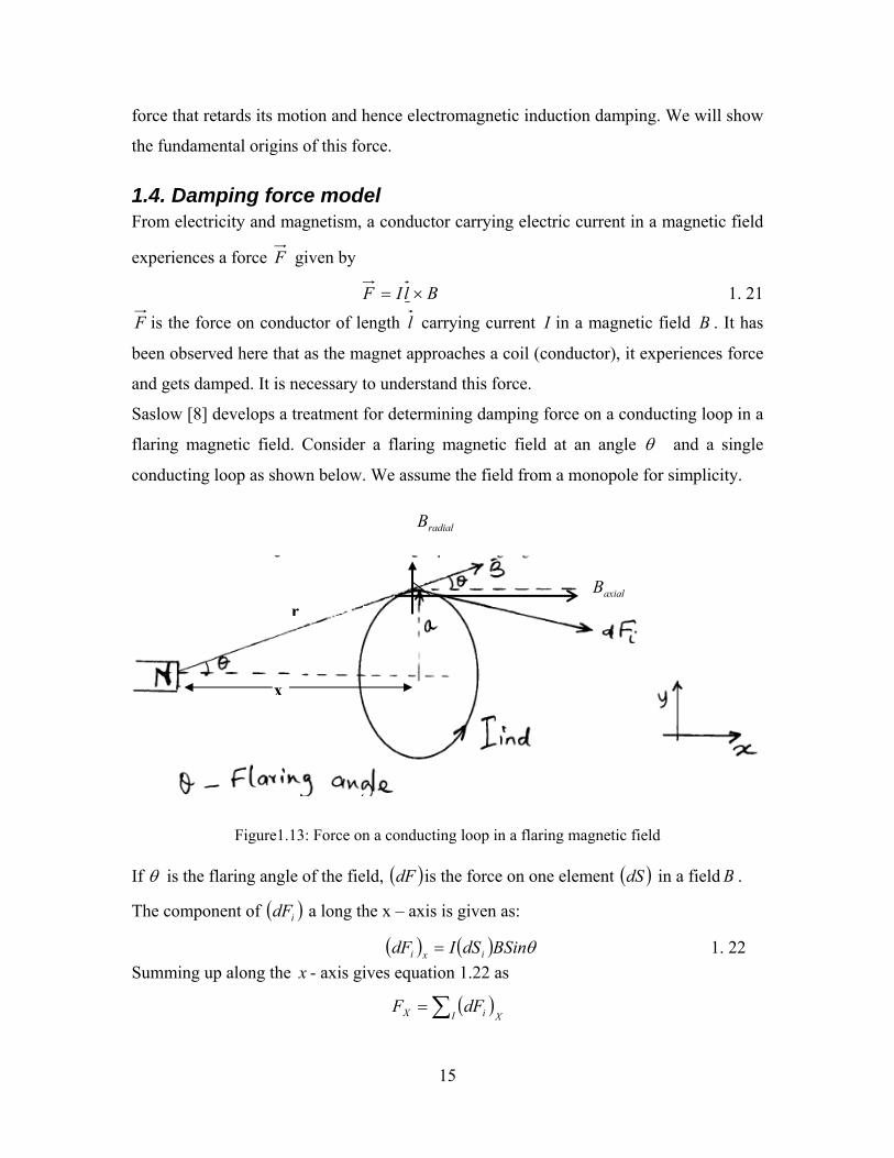
Saslow [8] develops a treatment for determining damping force on a conducting loop in a

flaring magnetic field. Consider a flaring magnetic field at an angle θ and a single

conducting loop as shown below. We assume the field from a monopole for simplicity.

Figure1.13: Force on a conducting loop in a flaring magnetic field If θ is the flaring angle of the field, ( )dF is the force on one element ( )dS in a field B .

The component of ( )idF a long the x – axis is given as:

( ) ( ) θBSindSIdF ixi = 1. 22 Summing up along the x - axis gives equation 1.22 as

( )XI iX dFF ∑=

x

raxialB

radialB

16

( )∑=i idSIBSinθ

( )aIBSin πθ 2=

( ) θπ BSinaIFloop 2= 1. 23

Where “a” is the coil radius and θ is the flaring angle.

Equation 1.23 represents force on a single loop or turn of wire in a flaring magnetic field.

However, for N turns of a coil, the total sum of the force is given as

( ) θπ BSinaNIF 2= 1. 24 The force varies with x because it comes from the interaction between the induced

current in the coil and the changing magnetic field gradient of the permanent magnet. The

x-displacement is changing and that means the equation 1.24 changes as follows:

( ) ( ) ( )xBxaINxF radπ2= 1. 25 One would expect the force in equation 1.24 to be, maximum at x = 0 since the radial

magnetic field is greatest there. At the same time induced current in the loop is expected

to be approaching zero then switch its sign. Since magnetic field B will be switching sign

as well, both current and magnetic field are negative or positive at the same time. In

essence, force which is now a product of either two negative values or two positive

values ends up positive throughout. Therefore, the force versus displacement graph takes

the shape shown below.

Figure 1. 14: Sketch of force versus displacement The two peaks above correspond to the peaks expected in the induced current versus time

graph. That means equation 1.24 has a maximum value given by

Forc

e

Displacement

17

aNIBF π2max = 1. 26 Equation 1.26 is the maximum force experienced by a coil of wire of N turns in a flaring

magnetic field as a magnet approaches a coil of wire. By substituting current, I from

equation 1.3, equation 1.26 changes as follows:

RVaNBFPEAK π2=

⎟⎠⎞

⎜⎝⎛=

dtdN

RNBa PEAK φπ2

⎟⎠⎞

⎜⎝⎛⎟⎠⎞

⎜⎝⎛=

dtdx

dxd

RBN

a PEAK φπ2

2 1. 27

Equation 1.27 has a coefficient of velocity term on the right hand side. So letting the

coefficient to be a constant makes the equation become

cvFPEAK = 1. 28

Where v is velocity and c is a constant of proportionality between maximum force and

velocity. The constant c is derived from Saslow’s equation 1.27. While force F and

velocity v are used extensively in most Physics and Engineering text books, it is often

phenomenologically based. We therefore expect a linear relation between damping force

and velocity when a magnet is put to vibrate at fixed frequencies in a coil of wire.

1.5 Forced Motion Various frequencies are to be chosen by adjusting the motor’s revolutions per minute.

The coils are to be placed on a force sensor to measure damping force. Damping force is

to be studied at different frequencies or velocities. However, before we look at forced

motion deeply, we need to study an E.M.I model. The model which comes from Saslow

Wayne [8] is to help us understand the phenomena of E.M.I in both free motion case and

forced damping case.

1.5.1. Damping force versus velocity The E.M.I coil is to be placed with its axis of rotation horizontal. Just like in section

1.2.2, the magnet is expected to be damped; the same is expected in this case. Also, as the

frequency of vibration increases, the magnet is expected to be damped higher because

18

velocity and frequency are directly proportional as shown below by equations 1.29, 1.30,

and 1.31 below. Induced voltage and velocity are directly proportional since at higher

magnet velocity time rate change of flux also goes higher. It is known that

rfv π2= 1. 29 Where v - is magnet’s linear velocity

r - is the crank radius

f - is the frequency of vibration

( )rfcF π2= 1. 30

Where F is damping force. From equation 1.30, it is expected that a plot of damping

force versus frequency gives a constant number. The constant number is expected to be

unique to every coil.

1.5.2. Damping force and power

The double and triple run coils as shown in Figure 2. 2 are expected to give different

induced currents and voltages depending on whether they connected in either parallel or

in series. It is expected that parallel connections give less resistance to induced current as

shown. Let us examine power output

22

22

eqeqeq R

dtdN

RVRiP

⎟⎠⎞

⎜⎝⎛

===

φ

1. 31

Where P is power, i is current, R is the equivalent resistance, N is number of turns, ρ is

the resistivity of the wire. Also we know from Physics that three coils of equal turns N

give effective turn as

Series 13 3NN S = and for parallel 13 NN P = . 1. 32 Based on the above, power in parallel and series become:

PR

dtdN

dtd

RNP

eq

SSeries 3

3

3 22

32

=⎟⎠⎞

⎜⎝⎛

=⎟⎠⎞

⎜⎝⎛=

φφ

1. 33

And PR

dtdN

Peq

parallel 3

3

22

1

=⎟⎠⎞

⎜⎝⎛

=

φ

1. 34

19

Power P in equations 1.34 and 1.35 are from equation 1.32. Both equations indicate that

power generated by the coils on either parallel or series connections are equal. We will

investigate this.

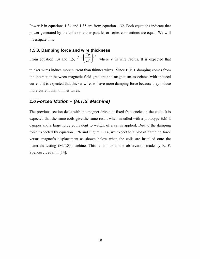
1.5.3. Damping force and wire thickness

From equation 1.4 and 1.5, 2r

lVI ⎟⎟

⎠

⎞⎜⎜⎝

⎛=

ρπ

where r is wire radius. It is expected that

thicker wires induce more current than thinner wires. Since E.M.I. damping comes from

the interaction between magnetic field gradient and magnetism associated with induced

current, it is expected that thicker wires to have more damping force because they induce

more current than thinner wires.

1.6 Forced Motion – (M.T.S. Machine) The previous section deals with the magnet driven at fixed frequencies in the coils. It is

expected that the same coils give the same result when installed with a prototype E.M.I.

damper and a large force equivalent to weight of a car is applied. Due to the damping

force expected by equation 1.26 and Figure 1. 14, we expect to a plot of damping force

versus magnet’s displacement as shown below when the coils are installed onto the

materials testing (M.T.S) machine. This is similar to the observation made by B. F.

Spencer Jr. et al in [14].

20

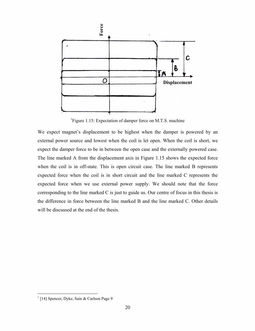
1Figure 1.15: Expectation of damper force on M.T.S. machine

We expect magnet’s displacement to be highest when the damper is powered by an

external power source and lowest when the coil is let open. When the coil is short, we

expect the damper force to be in between the open case and the externally powered case.

The line marked A from the displacement axis in Figure 1.15 shows the expected force

when the coil is in off-state. This is open circuit case. The line marked B represents

expected force when the coil is in short circuit and the line marked C represents the

expected force when we use external power supply. We should note that the force

corresponding to the line marked C is just to guide us. Our centre of focus in this thesis is

the difference in force between the line marked B and the line marked C. Other details

will be discussed at the end of the thesis.

1 [14] Spencer, Dyke, Sain & Carlson Page 9

Displacement

Forc

e

21

2 EXPERIMENTAL DETAILS

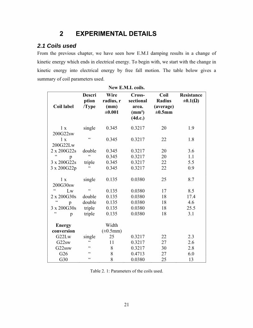
2.1 Coils used From the previous chapter, we have seen how E.M.I damping results in a change of

kinetic energy which ends in electrical energy. To begin with, we start with the change in

kinetic energy into electrical energy by free fall motion. The table below gives a

summary of coil parameters used.

New E.M.I. coils.

Table 2. 1: Parameters of the coils used.

Coil label

Description /Type

Wire radius, r

(mm) ±0.001

Cross-sectional

area. (mm²) (4d.c.)

Coil Radius

(average)±0.5mm

Resistance ±0.1(Ω)

1 x 200G22sw

single 0.345 0.3217 20 1.9

1 x 200G22Lw

“ 0.345 0.3217 22 1.8

2 x 200G22s double 0.345 0.3217 20 3.6 “ p “ 0.345 0.3217 20 1.1

3 x 200G22s triple 0.345 0.3217 22 5.5 3 x 200G22p “ 0.345 0.3217 22 0.9

1 x

200G30sw single 0.135 0.0380 25 8.7

“ Lw “ 0.135 0.0380 17 8.5 2 x 200G30s double 0.135 0.0380 18 17.4

“ p double 0.135 0.0380 18 4.6 3 x 200G30s triple 0.135 0.0380 18 25.5

“ p triple 0.135 0.0380 18 3.1

Energy conversion

Width (±0.5mm)

G22Lw single 25 0.3217 22 2.3 G22sw “ 11 0.3217 27 2.6 G22ssw “ 8 0.3217 30 2.8

G26 “ 8 0.4713 27 6.0 G30 “ 8 0.0380 25 13

22

Experiment 2.1 – Energy conversion. A cylindrical neodymium magnet of length 26mm, internal diameter 13mm, external

diameter 26mm and mass 89g was used. An identical non-magnetic piece of bronze of

mass of 91g was used to form an Atwood machine set up. The two pieces were

designated as 2m for the magnet and the piece of bronze solid as 1m . Both were

connected by an inextensible thread going round a pulley forming an Atwood machine

set up as shown below. The magnet was let to go through each coil of 200 turns. The coil

is made of copper wire wound on a P.V.C. The pulley used was a Pasco Rotary Motion

Sensor (PS-2120). It measures magnet’s placement and velocity with time and position.

Induced current is measured via Passport voltage-current sensor(PS-2115). Both the

voltage-current sensor and rotary motion sensor were connected to computer interface.

The data acquisition system (DAQ) used was Data studio 1.9.7r12. Together with this

DAQ software, the following could be measured at the same time for one run:

• Induced current with respect to time and magnet’s displacement.

• Magnet’s velocity with respect to displacement and time.

1Figure2. 1 Schematic diagram for the set up with a freely moving magnet Induced current was collected with the coils shorted to the ammeter. The table below

gives a summary of the E.M.I. coil parameters used.

1 Details of energy conversion are in appendix A.

Mass m1

Coil of wire of N turns

Rotary motion sensor

Magnet m2

23

Coil label Coil width

± 0.5(mm)

Wire thickness

± 0.001(mm)

22Lw 25 0.345

22sw 11 0.345

22ssw 8 0.345

30ssw 8 0.135

Table 2. 2: Summary of coil parameters.

Shorting the coils to the ammeter was geared towards getting the coil that converts most

percentage of the lost kinetic energy into electrical energy. The other data sets that follow

were considering other factors like the effect of coil width and wire thickness on

converting kinetic energy to into electrical energy.

2.1.1. Other factors In the previous work [10] uses only one type of wire. We investigated other factors to

investigate their effect on the percentage of energy converted. The factors investigated

include:

a) External load resistor.

b) Ratio of magnet length to coil width.

c) Thickness of the wire.

2.1.1.1. External resistor By considering coil resistance RC = (2.8±0.1Ω) different resistances were selected as

follows:

a) RL = 2.8Ω (RL = RC )

b) RL = 10 Ω ( RL > RC)

External resistances of (2.8±0.1) Ω and (10±0.1) Ω were connected at different times in

series with the coil of width 11mm and wire radius 0.345mm. The magnet was let to

traverse just like it was in the first case for short circuit. The same procedure for

experiment in section 2.1 was used to arrive at the results in section 3.1.

24

2.1.1.2. Ratio of magnet length to coil width Two coils of widths 25±0.5mm and 11±0.5mm had their readings taken at different times

with the same procedure as in the first case. Both were short through the ammeter.

2.1.1.3. Wire thickness Two coils of wire radii 0.345+0.001mm and 0.135±0.001mm had their readings taken

when short through the ammeter.

In all of the above investigations except in 2.1.1(b) for 10Ω external resistor,

measurements were done thrice then averaged.

2.2 Damping Force measurement Figure 2. 2 below shows an experimental set up that was used for the investigation of

damping force. E.M.I. damping was investigated and quantified in terms of:

(i) wire thickness

(ii) ratio of magnet length to coil width and

(iii) coil connection types.

We designed different types of E.M.I. coils as shown in Figure 2. 2 below. They can be

described as triple and double run coils respectively. The schematic diagram previously

seen in Figure1.4 refers to single run.

Figure 2. 2: E.M.I coil set ups used During the investigation, damping force was measured against velocity for different

coils.

25

Experiment 2.2 The magnet attached to an adjustable motor was set to vibrate back and forth inside an

E.M.I. coil placed with its axis of symmetry vertical on a Pasco Force sensor (CI-6537).

Force was collected via a Pasco analog adapter (PS-2158). Induced current was collected

from the pick coil via a Pasco voltage-current sensor (PS-2115) to the DAQ. Figure2. 3

below shows a circuit diagram used and Figure2.4 shows a picture of the same set up.

1Figure2. 3: Schematic diagram for investigating damping force. The Multimeter (Fluke 76) was used for setting up frequency of the motor by connecting

it to the pick up coil to read the frequency of the output signal from the coil. The motor

was adjusted for various integral frequencies from 2 Hz to 8 Hz. For each frequency,

damping force and induced current was measured simultaneously for each E.M.I. coil.

1 Other details of Experiment 2.2 are in Appendix B.

Multimeter

Force sensor

Magnet P.V.C

Coil of wire

S1

S2

Computer

Motor

Analog Adapter

Voltage-Current Sensor

26

Figure2.4: Damping force investigation Coils were grouped into two major categories: Single run coils in the first and then

double and triple runs in the other. Several coils as shown in Table3.1 were investigated.

2.3 Damping Force Model The experimental set up in Figure2. 1 was modified to take care of experimental

verification of E.M.I damping force.

Experiment 2.3 The whole set of apparatus from experiment 2.1 is brought to this experiment. A new coil

of 100 turns on a light P.V.C. was used unlike other coils in experiment 2.1 which had

very heavy coils. This experiment has a Hall probe to measure the radial magnetic field

as the magnet moves upwards. The right hand side of equation 1.26 is now completely

measured. The second modification as shown in Figure2. 5 is a P.V.C. tube to constrain

the magnet in one path as it moves upwards. This is because from equation 1.26, the

radial magnetic field varies strongly with the Hall probe position. There is need to ensure

that the magnet stays in one vertical position through out. So that means that the radial

field has to be averaged over thickness of the coil. To experimentally complete equation

Coil of wire in a P.V.C. case with

a magnet vibrating inside

Force sensor

Motor

27

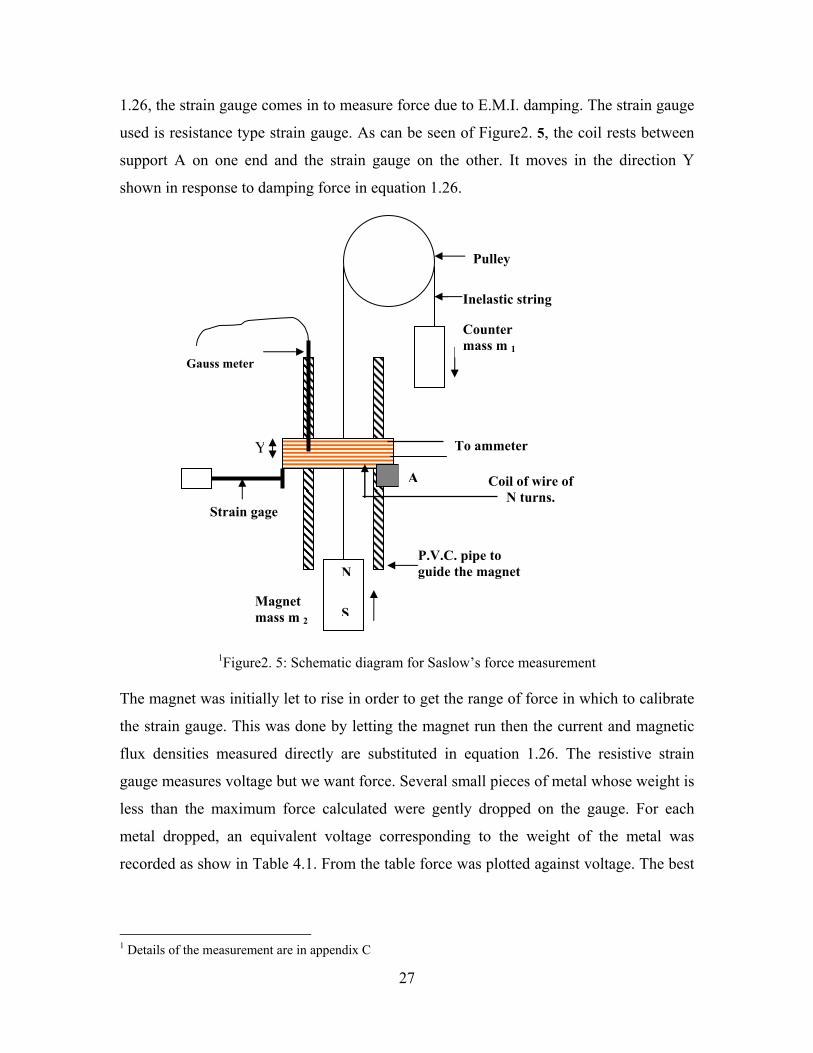
1.26, the strain gauge comes in to measure force due to E.M.I. damping. The strain gauge

used is resistance type strain gauge. As can be seen of Figure2. 5, the coil rests between

support A on one end and the strain gauge on the other. It moves in the direction Y

shown in response to damping force in equation 1.26.

1Figure2. 5: Schematic diagram for Saslow’s force measurement The magnet was initially let to rise in order to get the range of force in which to calibrate

the strain gauge. This was done by letting the magnet run then the current and magnetic

flux densities measured directly are substituted in equation 1.26. The resistive strain

gauge measures voltage but we want force. Several small pieces of metal whose weight is

less than the maximum force calculated were gently dropped on the gauge. For each

metal dropped, an equivalent voltage corresponding to the weight of the metal was

recorded as show in Table 4.1. From the table force was plotted against voltage. The best

1 Details of the measurement are in appendix C

N

Gauss meter

Strain gage

To ammeter

P.V.C. pipe to guide the magnet

Coil of wire of N turns.

Counter mass m 1

S

Pulley

Magnet mass m 2

Inelastic string

A

Y

28

line of fitting curve which converts voltage signals from the strain gauge into force was

then applied to our readings of the strain gauge.

During the time damping force was measured, we also considered induced voltage for the

same coil set ups when a large force equivalent to weight of a car is applied. This was

done by using a materials testing system (M.T.S) machine in the Mechanical engineering

laboratory. As it will be seen in section 3.2, different coil characteristics had different

observations.

2.4 Forced Motion - driven magnet (M.T.S. Machine) The materials testing system (M.T.S) machine uses Testware SX data acquisition

software different from DAQ used in the previous experiments. A prototype of an MR-

damper was mounted on M.T.S machine and E.M.I coils fitted below it a shown below.

Figure2.6: Single large width E.M.I coil installed

Figure2.7: EMI setup with triple coil installed

Figure2.6 and Figure2.7 above show two different types of E.M.I. coils installed on to an

M.T.S machine. Part of the study in this paper is energy maximization; different types of

Lower Cross head

Upper cross head

Single phase large width coil installed

MR - damper

29

E.M.I. coils were installed. The induced voltage was studied with respect to the following

factors.

(i) coil widths

(ii) connection types.

(iii) wire thicknesses.

Damping force was studied at three stages:

a) Off –state

b) E.M.I. coil short

c) External power.

In (a), each coil was left open and the magnet set to vibrate. Data was recorded for force

versus displacement. In (b), the coil was short. Likewise, force and displacement data

was recorded. This is when eddy current damping is maximum. In (c), external power

supply was used to supply a D.C. voltage of 4.0 V. At the same time electric current was

recorded as 0.2 A.

The machine was set to vibrate from frequencies of 0.5 Hz to 2 Hz due to mechanical

limitations. The results are discussed in section 3.3.

30

3 RESULTS AND DISCUSSION

3.1 Energy Conversion It was observed that as the magnet rises through the coil, it drags at a point below and

above the coil. This confirms observation made by R. Kingman et al [12] that maximum

induced voltage occurs at half the radius of the coil both below and above the coil. When

in the middle of the coil the magnet tends to restore its previous motion. The graph

shown in Figure3.1 (coil labeled 22sw) below represents typical results from one of the

coils. It is similar to our expectation as in Figure 1.7 and Figure 1. 8.

Square of Linear Velocity on displacement

0

0.05

0.1

0.15

0.2

0.25

0.3

0 0.1 0.2 0.3 0.4 0.5 0.6

Displacement (m)

Squa

re o

f vel

ocity

(m

/s)^

2

SQ. of Velocity

O

A

BC

DV^2 = 2as

d1 d2…. d110

E

Figure3.1: Square of Linear velocity against displacement

Part (A) – The magnet reaches the lower characteristic point. The repulsive force due to

an associated magnetism with induced current in the coil and the changing magnetic field

gradient of the magnet reaches maximum. The rising magnet decreases in acceleration.

Part (C) – The magnet reaches the middle of the coil where it undergoes free fall type of

motion but only for a very short time just before the magnet reaches the upper

characteristic point.

Part (B) – Is the upper characteristic point where the magnet experiences a force of

attraction due to associated magnetism of the induced current in the coil and the changing

magnetic field gradient.

31

The kinetic energy change is then found by substituting into equation 1.17 to give:

..EK∆ = ( ) ( )∑ −×+ 2221

121

OC VVn

mm 3. 1

= 21 (0.091kg +0.089kg) × (0.02907) J

= 2.61 millijoules of energy

Where n = 110, is the number of points averaged along the position axis. The converted

electrical energy is measured from the graph of the square of induced current against time

as shown in Figure3.3.

Induced current versus time

-6.00E-02

-4.00E-02

-2.00E-02

0.00E+00

2.00E-02

4.00E-02

6.00E-02

0 0.5 1 1.5 2

Time (s)

Indu

ced

curr

ent (

A)

Current ( A )

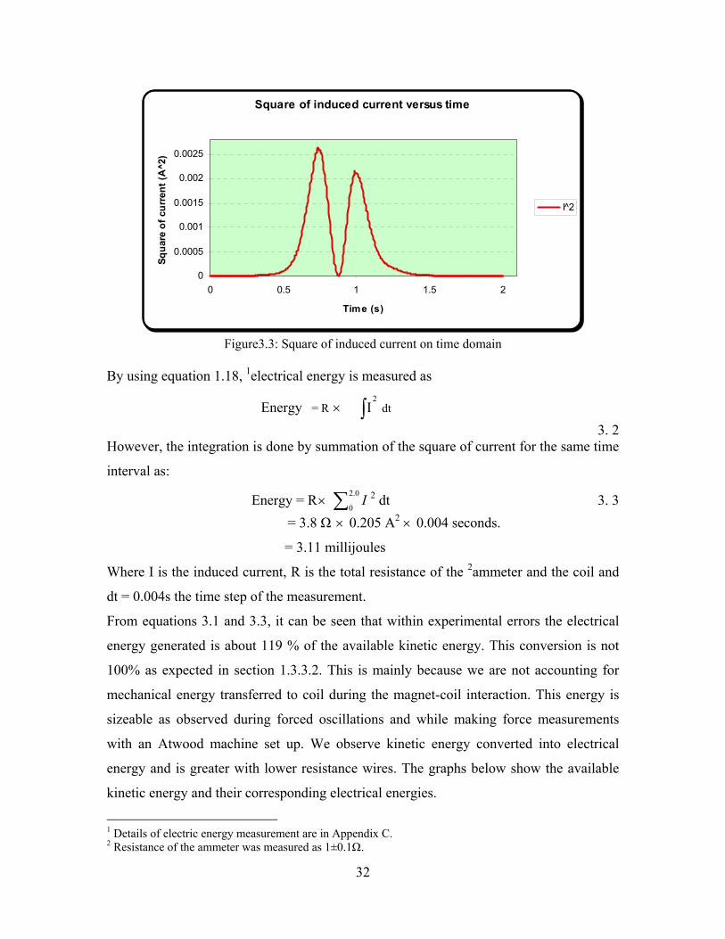
Figure 3.2: Induced current versus time When the current in Figure 3.2 is squared and plotted on time as Figure1.9 we get the

graph in Figure3.3 . It can be seen that the expected results concur with the experimental

results. Also, the expected curves in Figure1.9 concur with the results in Figure 3.2 and

Figure3.3.

32

Square of induced current versus time

0

0.0005

0.001

0.0015

0.002

0.0025

0 0.5 1 1.5 2

Time (s)

Squa

re o

f cur

rent

(A^2

)

I 2

Figure3.3: Square of induced current on time domain

By using equation 1.18, 1electrical energy is measured as

Energy = R × 2

I∫ dt 3. 2

However, the integration is done by summation of the square of current for the same time

interval as:

Energy = R× ∑ 0.2

0I 2 dt 3. 3

= 3.8 Ω × 0.205 A2 × 0.004 seconds.

= 3.11 millijoules

Where I is the induced current, R is the total resistance of the 2ammeter and the coil and

dt = 0.004s the time step of the measurement.

From equations 3.1 and 3.3, it can be seen that within experimental errors the electrical

energy generated is about 119 % of the available kinetic energy. This conversion is not

100% as expected in section 1.3.3.2. This is mainly because we are not accounting for

mechanical energy transferred to coil during the magnet-coil interaction. This energy is

sizeable as observed during forced oscillations and while making force measurements

with an Atwood machine set up. We observe kinetic energy converted into electrical

energy and is greater with lower resistance wires. The graphs below show the available

kinetic energy and their corresponding electrical energies.

1 Details of electric energy measurement are in Appendix C. 2 Resistance of the ammeter was measured as 1±0.1Ω.

33

V^2 G22Lw

-0.01

0.04

0.09

0.14

0.19

0 0.1 0.2 0.3 0.4

Displacement (m)

V2

(m/s

)2

Sq. of velocity

G22Lw

0

0.0005

0.001

0.0015

0.002

0.0025

0.003

0.0035

0.6 1.1 1.6

Time (s)

I^2

(A)^

2

I^2

Figure 3. 4:Energy change for G22Lw

G22ssw

00.050.1

0.150.2

0.250.3

0 0.1 0.2 0.3 0.4 0.5

Displacement (m)

V^2

(m/s

)^2

Sq. of velocity

34

G22ssw

0

0.0005

0.001

0.0015

0.002

0.0025

0.3 0.5 0.7 0.9 1.1 1.3 1.5

Time (s)

I^2

(A)^

2

I 2

Figure 3. 5: Energy change for G22ssw

G22sw

0

0.05

0.1

0.15

0.2

0.25

0 0.1 0.2 0.3 0.4 0.5

Displacement (m)

V^2

(m/s

)^2

SQ. of Velocity

G22sw

0

0.005

0.01

0.015

0.02

0.025

0.03

0.65 0.75 0.85 0.95 1.05 1.15

Time (s)

I2

(A)

2

I 2

Figure 3. 6: Energy change for G22sw

35

G30ssw

0

0.01

0.02

0.03

0.04

0.05

0 0.05 0.1 0.15 0.2 0.25

Displacement(m)

V^2

(m/s

)^2

v^2

G30ssw

0

0.0001

0.0002

0.0003

0.0004

0.0005

0.6 0.8 1 1.2 1.4 1.6

Time (s)

I^2

(A)^

2

I 2

Figure 3. 7: Energy change for G30ssw

Table3.1 gives a summary of the change in kinetic energies observed as electrical energies

for different coils. The column of percentage error was obtained by expressing the

standard deviation as a percentage of the percent of the lost kinetic energy seen as

electrical energy.

100..%

% ×=convertedEofK

Deviationerror

36

Coil label and wire radius

±0.001mm

Coil

width

±0.5mm

Resistance

± 0.1 Ω

∆ K.E.

(mJ)

Electrical

energy

(mJ)

% of

K.E. lost

&

observed

as Elect.

energy

%

Error

G22ssw

0.345

7 2.8 2.4459 2.9866 122 8

G30ssw

0.135

7 13 1.8453 1.6833 92 20

G22sw

0.345

11 2.6 2.2860 3.1500 137 3

G22Lw

0.345

25 2.3 2.5479 3.3643 132 6

Note: The above resistances exclude resistance of the ammeter (1 ± 0.1Ω)

Table3.1: Details of the coils investigated. Although we can not account for part of mechanical energy, Table3.1 above shows that

thicker wires are better than thinner wires in changes in kinetic energy within the

experimental uncertainties. This is because their resistances are lower than for thinner

wires. Lastly, the slope of OA and BD of Figure3.1 is theoretically given by substitution

into equations 1.9 and 1.16 as

2/2177.08.98991899122 sm

gggga =×⎟⎟⎠

⎞⎜⎜⎝

⎛+−

×= 3. 4

For the particular coil used in this sample the slopes were fitted to be 0.2047 and 0.2098

for after and before damping respectively. The two slopes deviate by 4.8% from the slope

in equation 3.4.

37

3.2. Other factors considered The results are given in three groups:

(i) External load resistor.

(ii) Ratio of magnet length to coil width.

(iii) Thickness of the wire.

3.2.1. External resistance.

The thicker wire of radius 0.345mm with the smallest coil width of 7mm was

connected to external resistors as:

(i) RL = 2.8 ± 0.1Ω (RL = RC )

(ii) RL = 10 ± 0.1Ω ( RL > RC)

The results as shown in Figure3. 8 below show induced current versus time for

different external resistances.

Induced Current and external load

-0.055

-0.035

-0.015

0.005

0.025

0.045

0 0.5 1 1.5 2

Time (s)

Cur

rent

(A)

Short circuit, 122%

RL = 2.8 ohms, 88%

RL = 10 ohms, 62%

1Figure3. 8: Induced current for different external resistances

It can be seen that induced current is maximum for no external resistance and

minimum for the biggest external resistor. This is because from Ohm’s law, resistance

is inversely proportional to current. Table3.1 below showing percentages of kinetic

energy converted as electrical energy:

The summary of the change in kinetic energy converted into electrical energy is

summarized in the table below 1 Coil labeled 22ssw was used in this investigation.

38

External resistance

∆ K.E. Elect. energy

% of K.E. converted into Elect.

energy

% Error

0 2.4459 2.9866 122 8 2.8 2.2149 1.8866 88 21 10 1.4764 0.915 62 13

Table 3. 2: Effect of external resistance

From the table, it can be observed that as the external resistance increases, the percentage

of kinetic energy converted into electrical energy reduces. This is because as the external

resistance increases, the induced current also reduces as observed in Figure3. 8 above.

Kinetic energy change come as a result of damping that comes due to the magnitude of

the induced current. Therefore if the induced current is higher, the energy change should

also be higher. The table shows how external resistance affects energy change.

Square of linear velocity versus position for different external loads.

0

0.01

0.02

0.03

0.04

0.05

0.06

0 0.05 0.1 0.15 0.2 0.25

Position (m)

Squ

are

of L

inea

r ve

loci

ty (m

/s)^

2

Short circuit, 122%

RL= 2.8 Ω, 88%

RL = 10 Ω, 62%

Figure3.9 : Kinetic energy change for different external loads.

From Figure3. 8, it can be seen that as external load increases, induced current decreases.

Therefore there is less E.M.I damping, resulting in almost no kinetic energy change as

shown in the curve of 10 Ω in Figure3.9 above. Also observed is that as the external load

increases the square of velocity graph approaches an open circuit situation where

39

resistance is maximum. According to [10], Power losses due to Joule heating effect are

calculated as

R

VP2

= 3. 5

Where V and R are induced voltage and resistance respectively. From equation 3.4 in

conjunction with the observation in Figure3.9, it can be seen that as the external

resistance increases, percentage of kinetic energy made available as electrical energy

decreases. The bigger the difference between the square of velocities as in equation 3.1,

the more the kinetic energy becomes available to be converted into electrical energy.

Therefore, a good vibration energy harvester should have the smallest possible external

resistance. In general, percentage of kinetic energy converted to electrical is low due

large uncertainties at low change in kinetic energy and to a smaller fraction of the initial

kinetic energy transferred to mechanical energy in the coil.

3.2.2. Ratio of magnet length to coil width In this paper, we investigated the above effect by having a fixed length 25mm of the

magnet with two different coil widths as shown in Figure 1. 11 while magnet widths were

25mm, and 7mm.The results for the effect of this ratio as already seen from the last two

rows in the column of kinetic energy change of Table3.1 which indicate that larger coil

widths convert more kinetic energy than smaller coil widths. This contradicts the

expectation made earlier in section 1.2.3.1. However, drawing conclusion in the coil

width from this investigation is hindered with the fact that there is a possibility of an

unaccounted for mechanical energy going into the coil but does not appear as electrical

energy.

3.2.3. Thickness of the wire. There wire radii investigated here were of 0.135mm and 0.345mm. The results in

Figure3.10 below indicates that a thicker wire induces more current also converts more

energy as had been seen in Table3.1.

40

Induced current and wire thickness

-0.055

-0.035

-0.015

0.005

0.025

0.045

0 0.5 1 1.5

Time (s)

Indu

ced

Cur

rent

(A)

r = 0.345mm, 122%

r = 0.135mm, 92%

Figure3.10: Induced and wire thickness for the same width

From Table3.1, it can be seen that the thicker wire has more kinetic energy change and

also coverts most. This comes because the induced current in thicker wire is more than

the thinner wire when the same voltage is applied. So the thicker wire causes more E.M.I

damping than the thinner wire.

3.3 Damping force –Atwood’s machine With reference to Figure2. 5, it was observed that as the magnet rises, damping force is so

large that one observes the coil being lifted upwards. Figure 3. 12 below shows the

measured force and also the calculated force when the Gauss probe was put both inside

and outside the coil. The force equation derived earlier is shown below.

( ) ( ) ( )xBxaNIxF radπ2=

From the force equation, the radial magnetic field versus time graph for both probe inside

and outside the coil is shown below.

41

Radial magnetic field and Current

-0.15

-0.1

-0.05

0

0.05

0.1

0.15

0.7 0.9 1.1 1.3

Time (s)

B-F

ield

(T) a

nd C

urre

nt (A

)

B -in (T)B-out (T)Current ( A )

Figure3.11: Radial magnetic field with induced current

The induced current in the coil gives rises to the radial magnetic field detected by the

Gauss meter. Because magnetic field is inversely proportional to the cube of distance, the

field detected when the Gauss probe is outside the coil is less than the field detected when

the Gauss probe inside the coil at any time. This can be observed in Figure3.11 above.

The assumption in the force equation is that the Gauss probe should be directly inside the

coil. This is not very possible. That is why the probe is put both inside and outside the

coil. The calculated values for both the probe in and out are then compared with the

measured value from the strain gauge which does not depend on the position of the Gauss

probe. The figure below shows the results of the theoretical and the experimental

measurement of the damping force.

42

Force

-0.03

-0.01

0.01

0.03

0.05

0.07

0.09

0.6 0.8 1 1.2 1.4 1.6

Time (s)

Forc

e (N

) F(measured)

F(calc. P-in)

F(calc. P-out)

Figure 3. 12: Theoretical and experimental measurements of Saslow’s force.

The results in Figure 3. 12 above are consistent with the expectations from the energy

diagrams in Figure1.12 and Saslow’s model. Also, it can be seen that the experimentally

measured force concurs with the calculated force within the limits of the resolution of the

instruments. Next, note that when the probe is outside the coil, it senses a smaller radial

magnetic field compared to when the probe is inside the coil. That explains why the

calculated force with probe inside is higher than when the probe is out.

The result in Figure 3. 12 portrays a lot of success in modeling of the damping force. It

shows clearly that when one uses the formula to calculate the damping force, the results

may not have much uncertainty. This is a very big help especially when one wants to

design a damper. A complete analytical modeling of the damping force would involve the

relation

( ) ( ) ( ) ( )yVdy

ydyBRaNyF ⎟⎟

⎠

⎞⎜⎜⎝

⎛=

φπ 22 3. 6

Where ( )⎟⎟⎠

⎞⎜⎜⎝

⎛dy

ydφ is the change of magnetic flux with position and ( )yV is the velocity.

The first significant step is already done with results in Figure 3. 12. The next step should

have measurements of flux change with respect to displacement as the magnet gets

damped. When peak value ( )yB is substituted in equation 3.6, the coefficient of the

43

velocity term on the right hand side of the equation should give coefficient of damping of

a coil as discussed in the next section. Finally, one could use equation 3.6 to model the

force entirely with computational techniques.

3.4 Damping force-Driven oscillations

3.4.1. Damping force and velocity. The force experienced by the magnet is proportional to its velocity as had been discussed

according equation 1.28. Plots of damping force against velocity for all the coils yield

straight line graphs whose slopes is are constant numbers called coefficient of damping

[9]. It has been found and confirmed that damping coefficient is unique for each coil as

had been expected. A typical graph of this kind is in the Figure 3. 13 below. The other

coefficients for other coils are tabled in Table3.3 .

Damping Force and Velocity for c.w.= 11mm

y = 0.657x - 0.213R2 = 0.9208

y = 0.1467x - 0.0306R2 = 0.8841

00.10.20.30.40.50.60.70.8

0 0.2 0.4 0.6 0.8 1 1.2 1.4

Linear Velocity (m/s)

Dam

ping

forc

e (N

)

r = 0.345mmr= 0.135mmLinear (r = 0.345mm)Linear (r= 0.135mm)

Figure 3. 13: Damping force and linear velocity

44

c.w.stands for coil width

Table3.3: Summary of damping coefficients of all the coils From the above table it can be seen that the thicker wire has more damping coefficient

than the thinner wire in all the three categories. This is because the thicker has less

resistance than the thinner wire. So induced current is more in the thicker wire resulting

in more damping force.

3.5 M.T.S Machine In this section of M.T.S. machine, induced voltage was investigated in relation to:

i. Coil widths ii. Connection types

When a large force as that of a car was applied to a prototype of an E.M.I damper.

3.5.1 Induced voltage and coil width. The magnet of length 26mm was set to vibrate at a frequency of 1 Hz with amplitude of

12.69mm. Recall from section 1.2.3.1 that when the coil width is very large, induced

voltage is reduced. This is observed to be consistent with the results shown in Figure3. 14

Coil Type

Coil Description

Resistance ±0.1 Ω

Damping Coefficient (kg/s)

R = 0.345mm, c.w.= 11mm 1.9 0.657

R = 0.345mm, c.w.= 25mm 1.8 0.516 R = 0.135mm, c.w = 11mm 8.7 0.147

Single

R = 0.135mm, c.w = 25mm 8.5 0.0788

R = 0.345mm, series 3.6 0.4869 R = 0.345mm, parallel 1.1 0.3679 R = 0.135mm, parallel 4.6 0.1302

Double

R = 0.135mm, series 17.4 0.05

R = 0.345mm, parallel 0.9 1.3147

R = 0.345mm, series 5.5 0.4237 R = 0.135mm, parallel 25.5 0.3147

Triple

R = 0.135mm, series 3.1 0.0207

45

below. It can be seen that a smaller coil width induces more voltage than the larger coil

width.

Induced voltage with coil width for r = 0.135mmf = 1 Hz, amplitude = 12.69mm

-0.12

-0.07

-0.02

0.03

0.08

0.13

2 2.5 3 3.5 4

Time (s)

Indu

ced

Volta

ge (V

)

Emf(c.w =25mm)

Emf(c.w =11mm)

Figure3. 14: Coil width factor for thinner wire in narrow and wider widths.

3.5.2 Induced voltage and connection type A magnet of length 26mm was set to vibrate at a frequency of 1 Hz with 12.69mm

amplitude in a three run coil of wire radius 0.345mm. The induced voltage was collected

when the three runs were in series and when in parallel. A plot of the induced voltage

versus time for the two types of connections as shown in Figure3.15.

Induced voltage for parallel and series connection types (triple run)

-0.016

-0.011

-0.006

-0.001

0.004

0.009

0.014

0 1 2 3 4

Time (s)

Indu

ced

volta

ge (V

)

Emf(series)Emf(parallel)

r = 0.345mm

Figure3.15: Induced voltage with connection type at 0.5 Hz frequency

It was observed as in that series type of connection gives more induced voltage than its

parallel counterpart. From Ohm’s law, induced current is inversely proportional to

46

resistance when other factors like voltage are kept constant. We have total resistance as

RRT 3= Ω and 3RRT = Ω for series and parallel circuit connections respectively

where R is resistance of each run of the coil. It can then be seen that the series

connection type has a bigger resistance hence more induced voltage than the parallel type

of connection.

3.6 Power – Vibrating magnet Power generated is given as RiP 2= where I is the induced current and R is the

resistance. Power generated was plotted against frequency with the results in the graphs

below

Power for single run coils.

0

0.1

0.2

0.3

0.4

0.5

1.8 3.8 5.8 7.8

Frequency (Hz)

Pow

er (W

)

G22sw

G22Lw

G30sw

G30Lw

Pow er (G22Lw )

Pow er (G22sw )

Pow er (G30sw )

Pow er (G30Lw )

Figure3.16: Power for single run coils

Power for 2 run coils

0

0.1

0.2

0.3

0.4

0.5

0.6

1.8 3.8 5.8 7.8

Frequency (Hz)

Pow

er (W

)

2xG30parallel2xG30series2xG22parallel2xG22seriesPower (2xG22series)Power (2xG22parallel)Power (2xG30parallel)Power (2xG30series)

Figure 3. 17: Power for double run coils

47

Power vs Frequency_ 3 run coils.

00.05

0.10.15

0.20.25

0.30.35

0.4

1.8 3.8 5.8 7.8

Frequency (Hz)

Pow

er (W

atts

) 3xG22series3xG22parallel3xG30series3xG30parallelPower (3xG30series)Power (3xG30parallel)Power (3xG22parallel)Power (3xG22series)

Figure 3. 18: Power for double run coils

In all the three sections above power generated increases in non-linearly with increase in

frequency. As frequency increases, velocity increases, flux change increases and hence

the induced current. Since Power is proportional to the square of the current a non-linear

relation is observed above.

According to our anticipation by equation 1.34, power generated by the double and triple

runs should not depend of the type of connection. This is however not observed in all the

cases at all the frequencies. At low frequencies, the anticipation is confirmed. As

frequency increases the discrepancy increases in all the coils.

3.7 Power – M.T.S Machine The following results were observed for different coils when damper force was plotted

versus displacement. Figure3. 19 shows the results of a wire of radius 0.345mm in a

wider coil width of 25mm when the magnet was set to vibrate at a frequency of 0.5 Hz

with amplitude of 0.5 inches (12.69mm).

48

Force

-5.5

-3.5

-1.5

0.5

2.5

4.5

-0.55 -0.35 -0.15 0.05 0.25 0.45

Displacement (in)

Forc

e (lb

f) F(offstate)

F(E.M.I.short)

F(4V dc)

amplitude = 0.5 inches

r = 0.345mm, c.w. = 25mm

Figure3. 19: Damper force for a thicker wire and a larger coil width It is very clear as had been expected that the force when the damper is powered externally

is larger than the force when the damper is powered internally. To asses the essence of

this thesis, we need to observe force when the damper is supplied with the energy from

its vibrations. Therefore, when the above is zoomed, we get the below figure.

Force

-0.9-0.7-0.5-0.3-0.10.10.30.50.70.9

-0.1 -0.05 0 0.05 0.1

Displacement (in)

Forc

e (lb

f)

F(offstate)

F(emishort)

f = 0.5 Hz

Figure3. 20: Details of damper force with displacement

From the zoomed graph, we observe that there is no clear cut difference in damper force

between off-state and coil short states at a frequency of 0.5 Hz. Because damping force

had been observed to be proportional to induced current which is proportional to

frequency, a plot of another coil at a frequency of 2 Hz is shown below.

49

Force

-1.1

-0.6

-0.1

0.4

0.9

1.4

-0.1 -0.05 0 0.05 0.1

Displacement (in)

Forc

e (lb

f)

Off-state

Coil short

f = 2 Hz, c.w. = 11mm

Figure3. 21: Damper force at higher frequency

It can be observed that at a higher frequency of 2 Hz, and a short coil width, there is still

no very clear cut difference between damper out put force in off-state and short coil state.

From the vibrating magnet results of the coils for example in Figure 3. 18, the average

power out put is 30mW. We observe a bigger damper output force as in Figure3. 19 when

the external power supplied to the damper as

mWAVPexternal 8002.00.4 =×= 3. 7

We know thatR

VP2

= . We assume the voltage of the coil used with the damper equals

the voltage of the same coil when short.

shortcoilMRIcoil VV ,, = 3. 8

So the power which the coil feeds into the damper in the M.T.S machine is given as

mWmWiR

RPP

mr

sshortMRI 53.3

8.2208.3

230

=⎥⎦⎤

⎢⎣⎡

Ω+ΩΩ

=⎟⎟⎠

⎞⎜⎜⎝

⎛×= 3. 9

1Where 20 Ω is the resistance of the damper, 2.8Ω is the coil’s resistance and 3.8 Ω is the

total resistance of the coil and the ammeter used in the vibrating magnet set up.

Comparing the two power values in equation 3.7 and 3.9 gives us

1 2 is used to convert peak current used earlier to rms current.

50

004.0800

53.3==

mWmW

PP

external

coil 3. 10

From equation 3.10, the power of the E.M.I. coil is about 0.4% of the external power

supply from our results. We can see that our coils supply less than 1% of the power that

the external power would supply. Therefore, for us to record the expected damper force

output, we need to increase the coil-magnet set up for more power output. Probably, the

damper used in this investigation requires higher induced current than the induced current

our E.M.I. coils could give out.

51

4 SUMMARY AND FUTURE WORK

Our investigations have been very successful especially on the damping force modeling.

The theoretical calculation clearly concurs with the measured force values despite the two

different positions of the Gauss meter. Actually, the radial magnetic field graphs with

induced current which causes E.M.I damping has come out so neatly to explain the

measured damping is never negative. It is well observed with the different Using our

findings, dampers can be designed

Based on the observations made in this paper within the limits of the resolution of the

instruments, a good electromagnetic induction damper should have:

i. Its coil made of thick wires

ii. Minimum external resistance

iii. Series type of connection with the coils when there is more than one

run.

Looking further on what is done on this paper, we have worked in high damping regime.

That is why at some point the electrical energy observed is more than the available

kinetic energy change which causes it. This shows there is some sizeable mechanical

energy we can not account for. For example, during the magnet-coil’s interaction the coil

itself gets some part of the energy transferred to it and some part goes through the coil

wire to be observed as electrical energy. In forced oscillations, the coil is well observed

to be trying to move off.

Therefore there is need for more work to be done to:

i. Account for the mechanical energy

ii. Mount the coil more rigidly

iii. To optimize the system to get more of the kinetic energy converted to

electrical energy.

For better results damper output force in the M.T.S machine, probably using a damper

with less power input requirement can yield better results. Conversely, a higher coil

magnet configuration would do better.

52

5 Reference: 1. B. O Gao: Hydro-Pneumatic Active Suspension. Department of Mechanical Engineering,

University of Bath, (Proceedings of the BRLSI Vol. 9, 2005)

(www.brlsi.org/proceed05/postgrad0505.html).

2. Young-Tai Choi and Norman M. Wereley - Self-Powered Magnetorheological

Dampers. (Proceedings of IMECE2006-1537, 2006 ASME International

Mechanical Engineering Congress and Exposition, Nov 5-10, 2006, Chicago,

Illinois, USA).

3. Suda Y, Nakano K., Nakadai S, Tsunashima H, Washizu T.: Self-Powered Active

Control Applied to a Cab Suspension, Source: JSAE Review, Volume

20, Number 4, October 1999 , pp. 511-516(6)Publisher: Elsevier

4. Kimihiko Nakano, Yashihiro Suba and Shigeyuki Nakadai: Self-Powered active

vibration control using a single electric actuator, Journal of Sound and Vibration,

Volume 260, Issue 2, p. 213-235.(Elsevier )(www.elsevier.cm/locate.jsv)

5. Douglas P. Taylor: Damper Retrofit of The London Millennium Footbridge – A

case study in biodynamic design.

6. Fishbane, Paul M et al: Physics For Scientists and Engineers, 2nd Ed.( Prentice-

Hall, New Jersey, 1996).

7. Nikhil S. Gujarathi, Rohit M. Ogle and Tarun Gupta: Production Capacity

analysis of a Shock absorber Assembly Line Using Simulation, Western Michigan

University, Kalamazoo, MI 49008, U.S.A (Proceedings of the 2004 Winter

Simulation Conference).

8. Saslow Wayne: Electricity, Magnetism and Light. (Thomson Learning, 2002)

9. Daniel J. Inman: Engineering Vibration, (Prentice-Hall, New Jersey, 1996).

10. Lowell T. Wood, Ray M. Rottmann, and Regina Barrera: Faraday's law, Lenz's

law, and conservation of energy. Am. J. Phys. 72, 376 (2004)

11. Randal D. Knight. Physics for Scientists and Engineers.(Pearson Education Inc.,

2004).

12. Kingman, Robert; Rowland, S. Clark; Popescu, Sabin, An experimental

observation of Faraday's law of induction. American Journal of Physics, Vol. 70,

Issue: 6, June 2002. pp. 595-598

53

13. John N. Fox and Daniel G. Reiber: Magnetic Induction and the Linear Air Track.

Am. J. Phys. 41, 75 (1973)

R. C. Nicklin Faraday's law—Quantitative experiments. Am. J. Phys. 54, 422

(1986).

14. B. F. Spencer Jr., S. J. Dyke, M. K. Sain, and J. D. Carlson: Phenomenological

Model for Magnetorheological Dampers. J. Engrg. Mech. 123, 230 (1997).

54

6 APPENDICES

6.1 Appendix A: Energy Change A cylindrical hollow magnet and a similar piece of bronze were connected by a string

that goes over the biggest pulley of a rotary force sensor. The coil radius of the coil of

wire used in this initial investigation was chosen according to [12] so that a significant

deviation of the induced voltage and current could be realized. The difference in mass

between the piece of bronze m2 and the magnet m1 was minimum so that the system is

kept at almost constant acceleration.

Measurements in Equations 3.1 and 3.3

The equations deal with kinetic energy change as the rising magnet interacts with the coil

of wire. The magnet was is set to start from rest at a fixed point below the coil. At the

same time, the data acquisition software was started. It was set to automatically stop after

a fixed time like 3.0 seconds. The following measurements were taken at the same time.

i. Induced current versus time

ii. Linear velocity versus displacement

The graph in Figure 4.1 below represents the paths traced by the magnet.

Square of Linear Velocity on displacement

0

0.05

0.1

0.15

0.2

0.25

0.3

0 0.1 0.2 0.3 0.4 0.5 0.6

Displacement (m)

Squ

are

of v

eloc

ity (

m/s

)^2

SQ. of Velocity

O

A

B

C

DV^2 = 2as

d1 d2…. d110

E

Figure 4.1: Kinetic energy change

Part OA represents magnet’s motion just before it begins to interact with the coil. This

part is extrapolated to E to represent the square velocity in the open circuit (V2O). Part BD

55

which is ideally parallel to OE represents the magnet’s motion after interacting with the

coil. It represents the square of velocity in the closed circuit (V2C). For each point the

displacement domain (d1, d2,d3,……….d110), there are two corresponding square of

velocities in the open and closed circuit paths. The difference in V2O and V2

C for each di

is then averaged over n, the number of possible points along the domain. In this case n

was 110 points. The kinetic energy equation in equation 3.1 above neglects rotational

kinetic energy of the pulley and the kinetic energy of the connecting string. These are:

(i) Rotational K.E. of the pulley is given as:

K.E rot = 21 × ﴾Ip × ω2p﴿ Joules.

But ω2 = (rv )2 = 20241.0

02907.0 where 0.02907 (m/s)2 is taken from equation 3.1, r is

the pulley radius.

K.E rot = 21× 1.35× 10-6kg.m2/s × 22

2

0241.0)/(02907.0

msm

= 21037.3 −× millijoules.

Where 1Ip and ωp are moment of inertia and angular velocity of the pulley

respectively.

(ii) Kinetic energy of the connecting string is given as:

K.Estring = ⎟⎠⎞

⎜⎝⎛

21

×λ× L× V2

= ⎟⎠⎞

⎜⎝⎛

21 × 5.3 ×10-5 kg/m ×1.21m×0.02907 (m/s)2

= 41032.9 −× millijoules.

Where λ and L are linear mass density and length of the string respectively. Due to the

small magnitude of the energies above, they can be neglected.

Caution – The choice of number of points along the displacement axis should be as close

as possible to point B so as to minimize the effects of gravitational pull. 1 The moment of inertia of the pulley is given by the manufacturer of the rotary force sensor.

56

Electrical energy measurement. From Figure3.3 integration was done by summing the square of induced current and then

performing calculation as in equation 3.3.

Current, G22 W = 7 mm, run 1 Time ( s )

Current ( A ) I²

0 0.00054 2.86E-

07 ∑I² = 0.20468618

0.004 0.00054 2.86E-

07 dt = 0.004 secs.

0.008 0.00054 2.86E-

07 Rc = 3.8 Ω

0.012 0.00054 2.86E-

07 Elect. Energy= 0.00311 Juoles

0.016 0.00054 2.86E-

07 = 3.11 millijoules

0.02 0.0011 1.21E-

06

0.024 0.00054 2.86E-

07

0.028 0.00054 2.86E-

07

Table 4.1: Electrical energy calculation

6.2 Appendix B: Damping Force The objective in this investigation is to study how electromagnetic induction damping

behaves in different coil set ups when a magnet in this case is set to vibrate horizontally.

The magnet was set to vibrate at specific frequencies for each E.M.I. coil. The procedure

below the diagram illustrates more.

57

Preliminary testing. a) Balancing the coil on the force sensor.

b) Set the data acquisition software to read induced current and force each on

time domain.

c) Place the coil on the force sensor.

d) Set the motor to rotate at low frequency of about 2 Hz. Close S2.Start the

data acquisition software. Study carefully the induced current curve on the

computer interface. It should come out resembling a sine curve.

e) Adjust the position of the coil forward and backward until a symmetrical

curve comes out for induced current. When the current is symmetrical, the

coil is balanced.

f) Short the coil to observe a change in the force graph.

g) Stop the motor.

Multimeter

Force sensor

Magnet P.V.C

Coil of wire

S1

S2

Computer

Motor

Analog Adapter

Voltage-Current Sensor

58

Taking data.

(i) Start the motor at low frequency. With S2 open, close S1 to read the frequency

of the induced the current signal. Adjust the motor speed for a particular

frequency like f = 2 Hz to start.

(ii) Open S1. Start the data acquisition system. Let the motor run for about 5

seconds. Observe that induced current graph is reading zero while force graph

shows a non-zero reading.

(iii) Close S2. Let the motor run for about 5 seconds more. Observe that the

induced current graph this time shows induced current reading. Force graph

shows bigger amplitude. Stop the motor, stop the data acquisition system.

(iv) Extract tables of current and force versus time then copy and paste to excel

page.

(v) Repeat steps (i) to (iv) for f = 3Hz, 4Hz …8Hz.

(vi) For each frequency, there is background force before S2 is closed when

current is still zero. After S2 is closed, induced current begins to exist, the

magnet begins to experience damping and the force sensor detects a larger

force as the figures below illustrate.

Figure4.2: Measurement of damping force

S2 open

S2 closed

59

Figure4.3: Induced current measurement

(vii) Using suitable calculations, determine the root mean square values of force

when S2 is open and when it is closed for each frequency. The difference is

the force due electromagnetic induction damping for each frequency.

(viii) Make a table showing force when S2 is open, when closed, net force and root

mean square current for each frequency. For each frequency, determine also

root mean square current.

6.3 Appendix C: Damping force model This section deals with experimental measurement of force due to electromagnetic

induction damping. A light coil with one hundred turns of wire was mounted on a support

A and strain gauge on one side as shown in Figure2. 5. The coil is well observed going up

and down as the magnet passes. The magnet was allowed to traverse the coil just like in

section 2.1. However, this time the data acquisition system was made to measure the

following with time:

a) Induced current - I

b) Magnetic field intensity – B

c) Strain signals from the strain gauge.

For each run of the magnet, all the above quantities were measured at the same time.

S2 open

S1 closed

60

Procedure used The magnet was initially let to run through the coil. Induced current and magnetic

field was recorded with Gauss probe inside the coil and in the second run, Gauss

meter probe was put outside the coil.

Strain gauge calibration. By using equation 1.26, force was calculated to determine the range of the expected

magnitudes of force.

Several masses whose weights were less than the maximum force from the

calculation were then used to calibrate the strain gauge. The calibration scale used is

shown below in Table 4.2

Mass Voltage Force (N)

0.75 0.0009 0.00751.01 0.0013 0.0101

1.3 0.0021 0.0131.43 0.002 0.01431.92 0.0032 0.01922.01 0.0024 0.02012.13 0.0025 0.02132.17 0.0026 0.02172.47 0.0038 0.02472.59 0.0032 0.02592.59 0.0027 0.02592.75 0.0041 0.0275

2.9 0.0037 0.0293.08 0.0034 0.03083.29 0.0045 0.03293.41 0.0042 0.03413.58 0.0054 0.03583.62 0.0037 0.03623.73 0.0055 0.03734.05 0.0056 0.04054.15 0.007 0.04154.79 0.0056 0.0479

Table4.2: Strain gauge calibration

The best line of fit that was used to fit voltage readings to force was

005.00322.6 += VForce , 2R = 0.8575

Where V is the voltage reading.

61

Caution

The strain gauge requires calibration at any time of measurement because it is sensitive to

strain.