characterization of discrete fracture networks and

CHARACTERIZATION OF DISCRETE FRACTURE NETWORKS ANDTHEIR INFLUENCE ON CAVEABILITY AND FRAGMENTATION

by

Roderick Nicolaas Tollenaar

B.A.Sc., The University of British Columbia, 2005

A THESIS SUBMITED IN PARTIAL FULFILLMENT OF THEREQUIREMENTS FOR THE DEGREE OF

MASTER OF APPLIED SCIENCE

in

THE FACULTY OF GRADUATE STUDIES

(Mining Engineering)

THE UNIVERSITY OF BRITISH COLUMBIA

December 2008

© Roderick Nicolaas Tollenaar, 2008

ABSTRACT

This thesis focuses on the use of Discrete Fracture Network (DFN) modeling to simulate

rock masses with different characteristics by varying fracture spacing, persistence and

dispersion, and assessing block instability without failure due to brittle fracture. The DFN

method was used together with block theory to assess block volumes, characterize block

shapes, evaluate block failure modes and estimate block size distributions in simulated ore

bodies. A model was built to simulate block caving and run tests of specific rock mass

parameters to evaluate their impact on caveability and fragmentation.

The potential of the Block Shape Characterization Method (BSCM) for evaluating the

block shape distribution within a rock mass was further confirmed, especially when used

with the DFN method. The stability of the generated blocks was evaluated based on the

factors of safety obtained from the FracMan stability analysis. The information gathered

during modeling suggested that of the variables analyzed, fracture persistence has the largest

influence on the generation of drawbell blocking block sizes. Qualitative similarities between

the apparent block volume and the blockiness character were observed and confirmed

previous studies. The results indicate that caveability in this model is most sensitive to

changes in fracture spacing.

This research indicates that DFN modeling has great potential for fragmentation

evaluation and determination, caveability assessment, and investigating the factors

influencing the caving process.

TABLE OF CONTENTS

ABSTRACT ii

TABLE OF CONTENTS iii

LIST OF TABLES v

LIST OF FIGURES vi

ACKNOWLEDGEMENTS ix

INTRODUCTION 11.1 Problem Statement 11.2 Research Objectives 21.3 Thesis Organization 2

2. LITERATURE REVIEW 42.1 Block Caving 4

2.1.1 Description 42.1.2 Brief History 62.1.3 Types of Caving and Advantages of the Method 7

2.2 Caveability Assessment 82.2.1 Empirical Methods 82.2.2 Numerical Methods 12

2.3 Fragmentation 162.4 The Discrete Fracture Network (DFN) 22

2.4.1 Fracture Size 232.4.2 Fracture Density and Spacing 262.4.3 Fracture Orientation 282.4.4 Fracture Spatial Model 302.4.5 Fracture Termination 31

2.5 BlockTheory 312.6 Chapter Summary 38

3. METHODOLOGY 403.1 Characteristics of the Model 403.2 Model Geometry 433.3 Model Parameters 46

3.3.1 Fracture Intensity (Spacing) 473.3.2 Fracture Dispersion 483.3.3 Fracture Persistence 50

3.4 Simulated Rock Mass Characterization 523.5 Chapter Summary 54

4. RESULTS AND ANALYSIS 564.1 Block Shape Characterization 56

III

4.2 Block Failure Mode .654.3 Block Size Distributions 764.4 Assessment of Apparent Block Volume 874.5 Block Areas and Block Volumes for Generated Models 954.6 Brief Analysis of the Effects of Stress on Stability 108

5. CONCLUSION AND RECOMMENDATIONS 1125.1 Conclusions 1125.2 Recommendations for Further Work 114

REFERENCES 116

APPENDIX 125

Java Application Code 125

iv

LIST OF TABLES

Table 2.1: Rock fragmentation sizes and their potential effects on caving operations (Laubscher,2000) 17

Table 2.2: Fracture data and derived input data for a DFN model (Staub et al, 2002). See section2.4.2 for definitions ofP10,P21 and P32 22

Table 2.3: Types of finite blocks identified Goodman and Shi’s (1985) 33Table 3.1: Description of values used for the variables in the fracture intensity analysis 47Table 3.2: Description of chosen values for intensity 48Table 3.3: Variables used for dispersion analysis with the orthogonal model 48Table 3.4: Variables used for dispersion analysis with the orthogonal model 49Table 3.5: Parameters used for persistence models with constant spacing 51Table 3.6: Set of parameters for persistence models with constant fracture count 51Table 3.7: Description of assumed persistence values 52Table 3.8: Summary of the conceptual models generated in this thesis 54Table 4.1: Values for failure modes for blocks generated during the spacing simulations 66Table 4.2: Values for failure modes for blocks generated during the dispersion simulations 68Table 4.3: Values for failure modes for blocks generated during the modified dispersion

simulations 70Table 4.4: Values for failure modes for blocks generated during the persistence with constant

spacing simulations 72Table 4.5: Values for failure modes for blocks generated during the persistence with constant

fracture count simulations 74Table 4.6: Modification of Laubscher’s (2000) description of rock fragmentation sizes and their

potential effects in caving operations. (1) Northparkes, (2) El Teniente, (3) Palabora.(Brown, 2005) 78

Table 4.7: Percentage of the total block volume generated in the spacing simulations for each ofthe classification groups 79

Table 4.8: Percentage of the total block volume generated in the dispersion simulations for eachof the classification groups 81

Table 4.9: Percentage of the total block volume generated in the modified dispersion simulationsfor each of the classification groups 82

Table 4.10: Percentage of the total block volume generated in the persistence with constantspacing simulations for each of the classification groups 84

Table 4.11: Percentage of the total block volume generated in the persistence with constantfracture count simulations for each of the classification groups 85

Table 4.12: Summary of the block size distributions for all simulations 87Table 4.13: Summary of the impact on caveability potential of the different modeled variables.107

V

LIST OF FIGURES

Figure 2.1: Cut away view of a block cave (Duplancic, 2001) 4Figure 2.2: Conceptual caving model developed by Duplancic and Brady (1999) 6Figure 2.3: Known operating and planned block and panel caving mines around the world

(modified after Brown, 2005) 7Figure 2.4: Laubscher’s (2000) caving chart incorporating the shape factor for caves with

different geometries 9Figure 2.5: Adjustment factors in the Mathews stability method (Mathews et al., 1980) 10Figure 2.6: Mathews stability graph (Mathews et al., 1980; Brown, 2003) 11Figure 2.7: Extended Mathews stability graph based on logistic regression showing the stable

and caving lines (Mawdesley 2002) 12Figure 2.8: Modified block shape diagram (Kalenchuk et al., 2007a) illustrating how BSCM

classifies various shapes 21Figure 2.9: Discontinuities intersecting a circular sampling window in 3 ways; a) both ends

censored, b) one end censored, and c) both ends observable (Zhang and Einstein,1998) 25

Figure 2.10: Random intersections along a line produced by variable discontinuityorientations (Priest, 1993) 28

Figure 2.11: Schmidt equal area, lower hemisphere stereonets representing three fracture setsdisplaying the effects of different Fisher distributions. (a) K =8, (b) K =50 29

Figure 2.12: Example of DFN models generated using different fracture spatial models forequivalent fracture orientation and radius distributions. (a) Enhanced Baechermodel, (b) Nearest-Neighbour model and (c) Fractal Levy-Lee model (Elmo et al.,2007b) 31

Figure 2.13: Description of the block types identified by Goodman and Shi (1985) asdepicted in Table 2.3 34

Figure 2.14: Application of block theory using a spherical projection (Priest, 1993) 36Figure 2.15: Example of tunnel stability analysis performed with UNWEDGE (Rocscience,

2007) 37Figure 3.1: Comparison between UNWEDGE and FracMan stability analysis for a tunnel and

three joint sets. (a) UNWEDGE model for tunnel and three joint sets, (b) FracManmodel and stability analysis for tunnel and three joint sets 42

Figure 3.2: Model layout 43Figure 3.3: Schmidt equal area, lower hemisphere stereonet representing the three orthogonal

fracture sets used in the simulations. a)Original orthogonal model, b)Modifiedorthogonal model 44

Figure 3.4: Block with clipped fractures 45Figure 3.5: Sample model showing blocks generated after analysis 46Figure 3.6: Selected Schmidt equal area, lower hemisphere stereonets representing three

fracture sets with varying dispersion for the orthogonal model. a) i = 8, b) K 20,c) K = 50, d) K = constant 49

Figure 3.7: Selected Schmidt equal area, lower hemisphere stereonets representing threefracture sets with varying dispersion for the modified orthogonal model. a) K = 8,b) K = 20, c) K = 50, d) K = constant 50

Figure 3.8: Quantification of GSI chart (Cai et al., 2004) with red arrow outlining the rangeof block sizes that are expected to be generated from the modeling 53

vi

Figure 4.1: Block shape diagrams and block shape distribution plots for spacing simulations.58

Figure 4.2: Block shape diagrams and block shape distribution plots for dispersionsimulations 60

Figure 4.3: Block shape diagrams and block shape distribution plots for modified dispersionsimulations 61

Figure 4.4: Block shape diagrams and block shape distribution plots for persistencesimulations with constant spacing 63

Figure 4.5: Block shape diagrams and block shape distribution plots for persistencesimulations with constant fracture count 64

Figure 4.6: Failure modes for blocks generated during the spacing simulations. (a) Failuremode as percentage of total block volume. (b) Failure mode as percentage of totalnumber ofblocks 67

Figure 4.7: Failure modes for blocks generated during the dispersion simulations. (a) Failuremode as percentage of total block volume. (b) Failure mode as percentage of totalnumber ofblocks 69

Figure 4.8: Failure modes for blocks generated during the modified dispersion simulations.(a) Failure mode as percentage of total block volume. (b) Failure mode aspercentage of total number of blocks 71

Figure 4.9: Failure modes for blocks generated during the persistence with constant spacingsimulations. (a) Failure mode as percentage of total block volume. (b) Failuremode as percentage of total number of blocks 73

Figure 4.10: Failure modes for blocks generated during the persistence with constant fracturecount simulations. (a) Failure mode as percentage of total block volume. (b)Failure mode as percentage of total number ofblocks 75

Figure 4.11: Average block size distribution chart for spacing simulations 80Figure 4.12: Average block size distribution chart for dispersion simulations 81Figure 4.13: Block size distribution chart for modified dispersion simulations 83Figure 4.14: Block size distribution chart for persistence with constant spacing simulations.

84Figure 4.15: Block size distribution chart for persistence with constant fracture count

simulations 86Figure 4.16: (a) Apparent block volume against persistence factor for persistence simulations

with constant spacing of 2m, (b) Blockiness character against persistence factorfor persistence simulations with constant spacing of 2m 89

Figure 4.17: (a) Apparent block volume against spacing for spacing simulations withconstant persistence of 7m, (b) Blockiness character against spacing factor forspacing simulations with constant persistence of 7m 90

Figure 4.18: (a) Apparent block volume against persistence factor for persistence simulationswith constant fracture count, (b) Blockiness character against spacing factor forpersistence simulations with constant fracture count 91

Figure 4.19: (a) Apparent block volume against persistence factor for varying dispersionsimulations with constant persistence of 7m and constant spacing of 2m, (b)Blockiness character against spacing factor for spacing simulations with theoriginal orthogonal model, constant persistence of 7m and constant spacing of2m 93

VII

Figure 4.20: (a) Apparent block volume against persistence factor for varying dispersionsimulations with the modified orthogonal model, constant persistence of 7m andconstant spacing of 2m, (b) Blockiness character against spacing factor forspacing simulations with constant persistence of 7m and constant spacing of 2m.

94Figure 4.21: View of the undercut for model M2. Red areas represent unstable blocks and

green areas represent stable blocks 96Figure 4.22: Three dimensional view of the blocks generated for model M2. Red blocks are

unstable and green blocks are stable 97Figure 4.23: a) Total block area and total unstable block area plotted against spacing as a

percentage of total undercut area, b)Total block volume and total unstable blockvolume plotted against spacing as a percentage of total ore body volume 99

Figure 4.24: a) Total block area and total unstable block area plotted against dispersion(original and modified) as a percentage of total undercut area, b)Total blockvolume and total unstable block volume plotted against dispersion (original andmodified) as a percentage of total ore body volume 102

Figure 4.25: a) Total block area and total unstable block area plotted against persistence as apercentage of total undercut area for persistence models with constant spacing,b)Total block volume and total unstable block volume plotted against persistenceas a percentage of total ore body volume for persistence models with constantspacing 104

Figure 4.26: a) Total block area and total unstable block area plotted against persistence as apercentage of total undercut area for persistence models with constant fracturecount, b)Total block volume and total unstable block volume plotted againstpersistence as a percentage of total ore body volume for persistence models withconstant fracture count 106

Figure 4.27: Basic tunnel model used for UNWEDGE simulations. In this case modeling anasymmetrical block 109

Figure 4.28: Factors of safety for the different block shapes tested for a principal stress ratioof 1:1:1 110

Figure 4.29: Factors of safety for the different block shapes tested for a principal stress ratioof 2:1.5:1 110

Figure 4.30: Factors of safety for the different block shapes tested for a principal stress ratioof2:1:1 111

Figure 4.31: Factors of safety for the different block shapes tested for a principal stress ratioof2:2:1 111

VIII

ACKNOWLEDGEMENTS

First of all, I would like to thank my parents and my aunt Marjolijn for all the

encouragement and support they gave me whilst I was performing this research. Without

them, the task of completing my thesis would have been impossible.

I would like to thank my supervisors and committee members Dr. Scott Dunbar, Dr. Erik

Eberhardt and Dr. Doug Stead for their guidance and encouragement throughout all these

months of research. They also suggested my research topic and organized the project. They

spent many hours reviewing my work, providing me with ideas and suggestions for

improving my thesis. Thank you also for always keeping an open door for me, and for all the

hours of individual instruction and discussion.

I would like to thank Rio Tinto, especially Allan Moss, and NSERC for their funding

and support. Steve Rogers from Golder Associates for making FracMan Geomechanics

available to me; without FracMan this research would have been impossible. AMEC Earth

and Environmental, especially Stu Anderson, Drum Cavers, Michael Davies, Steve Rice and

Jan van Pelt, for their support and encouragement, and for allowing me to use all AMEC’s

facilities and resources. Simon Fraser University generously opened its doors to me and let

me use its facilities and computers to conduct my modeling.

Davide Elmo helped me a great deal with the FracMan modeling, as well as with the

ternary diagrams. I consider him my fourth supervisor. Wayne Gray provided the Java

knowledge in order to code my algorithms. Finally, I would like to thank my lab mates

Matthieu Sturzenegger, Alex Vyazmensky and David van Zeyl for their friendship, help, the

interesting discussions and the good laughs.

ix

1.0 INTRODUCTION

1.1 Problem Statement

In recent years, the mining industry has been faced with a fresh array of old and new

challenges. These include aging mines (most of which are surface mines), deeper deposits,

lower grades and an increase in demand for mineral resources. The block caving mining

method has emerged as an answer to many of these problems. It allows mining of massive,

low grade deposits at depth, and has the lowest production costs and the highest production

rates of any underground mining method used today. It also provides high levels of safety for

the personnel and a good platform for automation. However, recent experiences in some

block cave operations around the world, such as Northparkes in Australia and Palabora in

South Africa, have highlighted the lack of understanding of the geotechnical processes

involved in caving. Among the most important factors in block cave mines are fragmentation

and caveability. Poor estimation of both of these variables can lead to production and

processing problems, or in the worst scenario, failure of the project.

In order to gain more understanding of the caving process, research was undertaken in

this thesis to study fragmentation and caveability. The investigation focussed on the use of

Discrete Fracture Network (DFN) modeling to simulate rock masses with different

characteristics by varying fracture spacing, persistence and dispersion, and assessing block

instability without failure due to brittle fracture. DFN modeling is a technique of fracture

simulation which allows the generation of three dimensional, synthetic fractures. The method

first saw use in the characterization of permeability of fractured rock masses and generic

studies on fracture influences. More recently it has been used as a tool in mining for rock

mass characterization, either by itself or together with other methods (e.g. synthetic rock

I

masses). In this thesis, the DFN method was used together with block theory (Goodman and

Shi, 1985) to assess block volumes, characterize block shapes, evaluate block failure modes

and estimate block size distributions in the simulated ore bodies.

1.2 Research Objectives

The key objectives of this thesis were as follows:

1. Characterize the block shapes generated with DFN models by varying fracture

intensity, persistence and dispersion;

2. Evaluate the block failure modes with different fracture spacing, persistence and

dispersion;

3. Investigate the effects on block size distribution of fracture intensity, persistence and

dispersion with DFN models and block theory;

4. Relate block volumes obtained from the models with the apparent block volume;

5. Study trace block areas (on the undercut) and block volumes for the generated

models.

1.3 Thesis Organization

Chapter 1 describes the problem and outlines the research objectives.

Chapter 2 presents a literature review on block caving as a mining method, the methods

currently employed for evaluating caveability and fragmentation, as well as describing the

Discrete Fracture Network method and Block Theory.

Chapter 3 explains the methodology used to complete this research, describing the

variables, model and procedure followed to accomplish the objectives.

2

Chapter 4 presents the results and analysis of the modeling performed.

Chapter 5 summarizes the conclusions of this research and gives recommendations for

future work.

3

2.0 LITERATURE REVIEW

2.1 Block Caving

2.1.1 Description

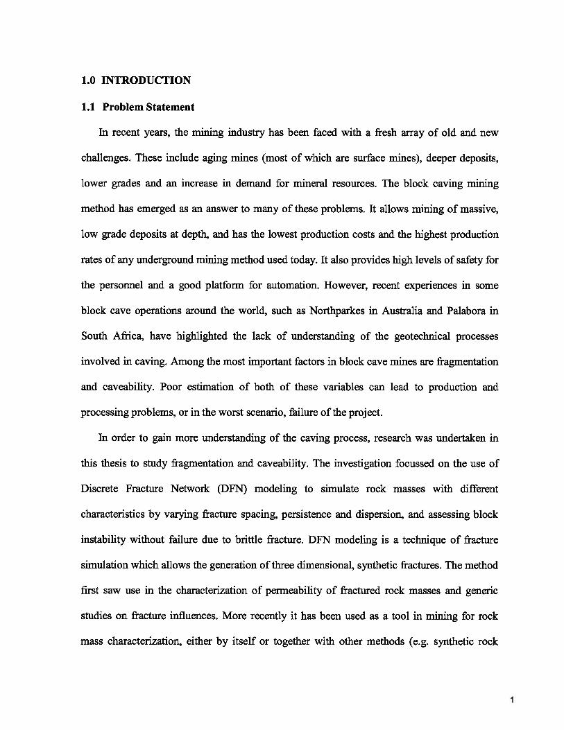
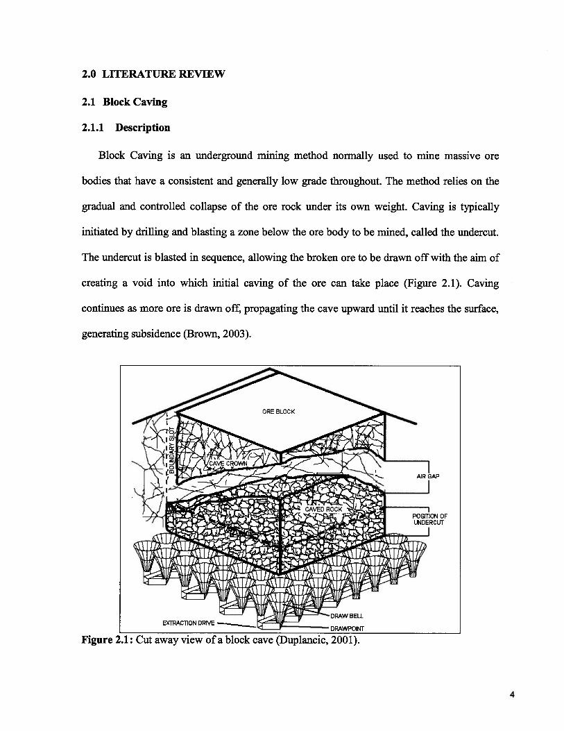
Block Caving is an underground mining method normally used to mine massive ore

bodies that have a consistent and generally low grade throughout. The method relies on the

gradual and controlled collapse of the ore rock under its own weight. Caving is typically

initiated by drilling and blasting a zone below the ore body to be mined, called the undercut.

The undercut is blasted in sequence, allowing the broken ore to be drawn off with the aim of

creating a void into which initial caving of the ore can take place (Figure 2.1). Caving

continues as more ore is drawn off, propagating the cave upward until it reaches the surface,

generating subsidence (Brown, 2003).

Figure 2.1: Cut away view of a block cave (Duplancic, 2001).

4

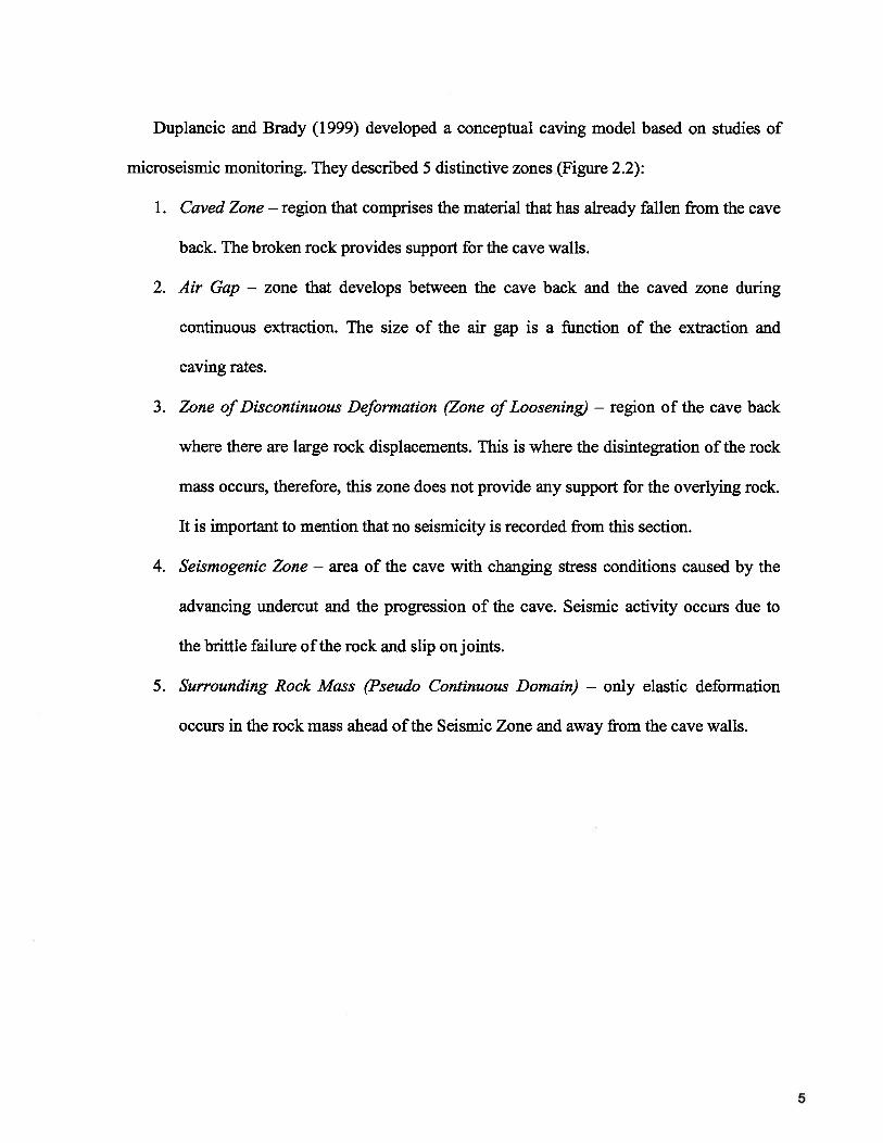
Duplancic and Brady (1999) developed a conceptual caving model based on studies of

microseismic monitoring. They described 5 distinctive zones (Figure 2.2):

1. Caved Zone — region that comprises the material that has already fallen from the cave

back. The broken rock provides support for the cave walls.

2. Air Gap — zone that develops between the cave back and the caved zone during

continuous extraction. The size of the air gap is a function of the extraction and

caving rates.

3. Zone of Discontinuous Deformation (Zone of Loosening) — region of the cave back

where there are large rock displacements. This is where the disintegration of the rock

mass occurs, therefore, this zone does not provide any support for the overlying rock.

It is important to mention that no seismicity is recorded from this section.

4. Seismogenic Zone — area of the cave with changing stress conditions caused by the

advancing undercut and the progression of the cave. Seismic activity occurs due to

the brittle failure of the rock and slip on joints.

5. Surrounding Rock Mass (Pseudo Continuous Domain) — only elastic deformation

occurs in the rock mass ahead of the Seismic Zone and away from the cave walls.

5

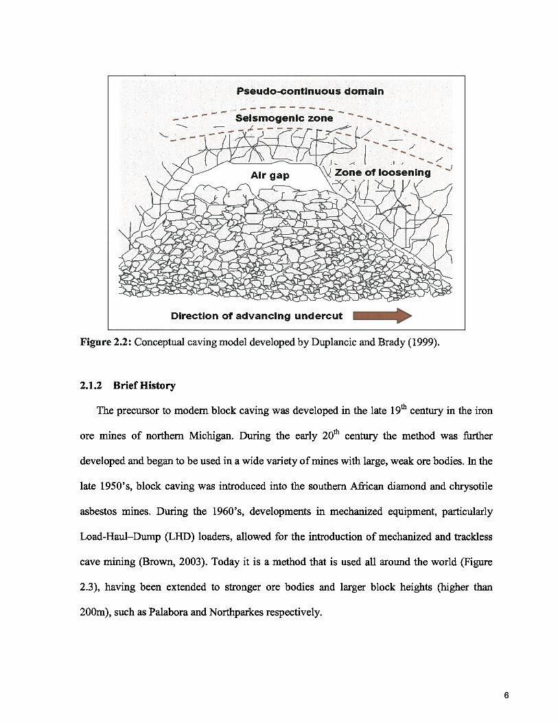
Figure 2.2: Conceptual caving model developed by Duplancic and Brady (1999).

2.1.2 Brief History

The precursor to modem block caving was developed in the late l9 century in the iron

ore mines of northern Michigan. During the early 20th century the method was further

developed and began to be used in a wide variety of mines with large, weak ore bodies. In the

late 1950’s, block caving was introduced into the southern African diamond and chrysotile

asbestos mines. During the 1960’s, developments in mechanized equipment, particularly

Load-Haul—Dump (LHD) loaders, allowed for the introduction of mechanized and trackless

cave mining (Brown, 2003). Today it is a method that is used all around the world (Figure

2.3), having been extended to stronger ore bodies and larger block heights (higher than

200m), such as Palabora and Northparkes respectively.

Pseudo-continuous domain

Seismogenic zone —

Direction of advancing undercut

6

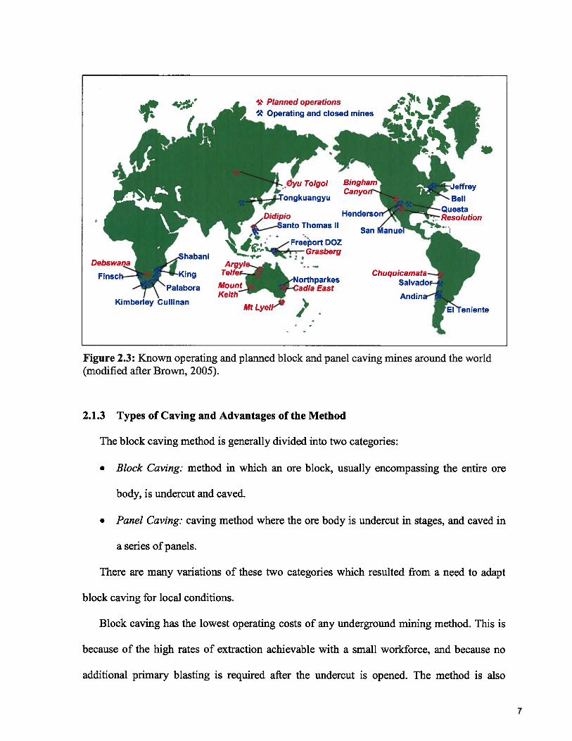
Figure 2.3: Known operating and planned block and panel caving mines around the world(modified after Brown, 2005).

2.1.3 Types of Caving and Advantages of the Method

The block caving method is generally divided into two categories:

• Block Caving: method in which an ore block, usually encompassing the entire ore

body, is undercut and caved.

• Panel Caving: caving method where the ore body is undercut in stages, and caved in

a series of panels.

There are many variations of these two categories which resulted from a need to adapt

block caving for local conditions.

Block caving has the lowest operating costs of any underground mining method. This is

because of the high rates of extraction achievable with a small workforce, and because no

additional primary blasting is required after the undercut is opened. The method is also

j’ Planned operations k

Operating and closed mines

Oyu Tolgoih’-Tongkuangyu

r Didipioanto Thomas II

BinghanCanyon’-’

TBeU4—QuestaHendersoiY/

— Resolution/

San Manuel’ —

DebswanaShabani

Finsch -King

Palabora

Kimberley Cullinan

rN0pMount rCadia EastKeith —

Mt Lyell

Chuquicamata—SalvadoF_j

Andina-

7

considered one of the safest, since most of the operations are conducted in the production

level with little personnel (Duplancic, 2001), i.e. there are no workers in stopes and they are

away from the caving zone.

2.2 Caveability Assessment

Caveability assessment methods are generally classified into two groups: empirical and

numerical.

2.2.1 Empirical Methods

Empirical methods have been developed from large amounts of data (based on previous

caving experience) and assumptions about its significance. This leads to the disadvantage,

though, that these methods have difficulty combining different variables in a simple robust

tool (Brown, 2003). The empirical methods used for block caving prediction include:

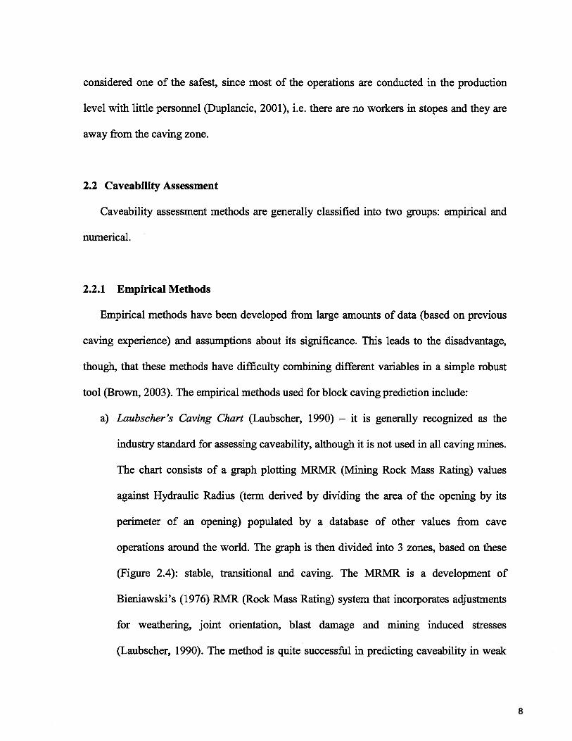
a) Laubscher ‘s Caving Chart (Laubscher, 1990) — it is generally recognized as the

industry standard for assessing caveability, although it is not used in all caving mines.

The chart consists of a graph plotting MRMR (Mining Rock Mass Rating) values

against Hydraulic Radius (term derived by dividing the area of the opening by its

perimeter of an opening) populated by a database of other values from cave

operations around the world. The graph is then divided into 3 zones, based on these

(Figure 2.4): stable, transitional and caving. The MRIVIR is a development of

Bieniawski’s (1976) RMR (Rock Mass Rating) system that incorporates adjustments

for weathering, joint orientation, blast damage and mining induced stresses

(Laubscher, 1990). The method is quite successful in predicting caveability in weak

8

and large ore bodies. However, it has shown limitations when applied to stronger

rocks and smaller footprints.

100 -

90

80

70

60

MR 50MR

40

30

2;L0

10

1 14

transitional

SCainng —a..

Curve A

Curve B

Ax 1.2

0 10 20 30 40 50Hydraulic radius

60 70 80m

150mx75mHR=25

Shape>1.5:1 curve-A

Figure 2.4:different geometries.

SHAPE FACTORstresses

oorn)

Shapel+/-30%:1 curve-B

Laubscher’s (2000) caving chart incorporating the shape factor for caves with

9

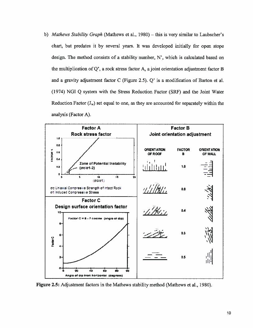
b) Mathews Stability Graph (Mathews et al., 1980) — this is very similar to Laubscher’s

chart, but predates it by several years. It was developed initially for open stope

design. The method consists of a stability number, N’, which is calculated based on

the multiplication of Q’, a rock stress factor A, a joint orientation adjustment factor B

and a gravity adjustment factor C (Figure 2.5). Q’ is a modification of Barton et al.

(1974) NGI Q system with the Stress Reduction Factor (SRF) and the Joint Water

Reduction Factor (J) set equal to one, as they are accounted for separately within the

analysis (Factor A).

Factor A Factor BRock stress factor Joint orientation adjustment

/ ORIENTATiON FACTOR ORIENTATiON

/ OF ROOF B OF WALL04 /

/ Zone of Potential Instabihty I

02 Cc’1-2) I iIiIiii1 1.0

010 I; —

cc’a1

ac Uniaxial Ccmprsi’e trergt cf Intact Rcck , 08ci lrce Ccmpraive Stress / / I ff/1/ f

Factor CDesign surface orientation factor

_______

0.4 9Facto C 8 -1 o.rne (.ongle 00 dIp)

S

AnGIe of dip Tron horIZ0rtaI (d.gres)

Figure 2.5: Adjustment factors in the Mathews stability method (Mathews et al., 1980).

10

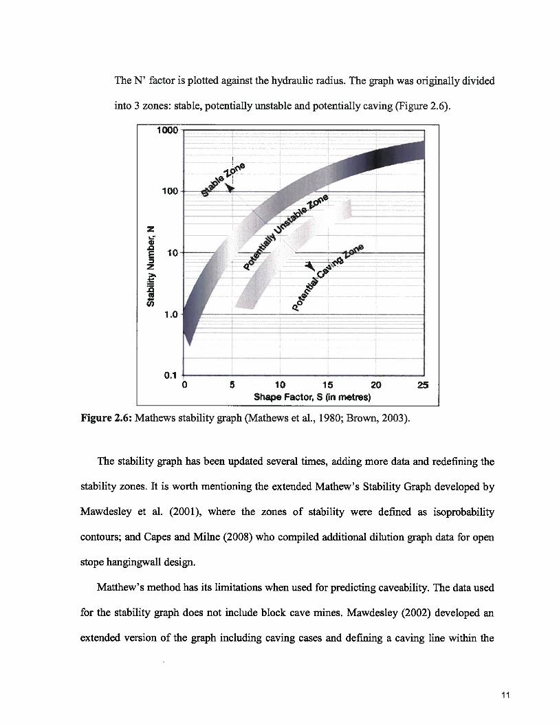
The N’ factor is plotted against the hydraulic radius. The graph was originally divided

into 3 zones: stable, potentially unstable and potentially caving (Figure 2.6).

Figure 2.6: Mathews stability graph (Mathews et al., 1980; Brown, 2003).

The stability graph has been updated several times, adding more data and redefining the

stability zones. It is worth mentioning the extended Mathew’s Stability Graph developed by

Mawdesley et al. (2001), where the zones of stability were defined as isoprobability

contours; and Capes and Mime (2008) who compiled additional dilution graph data for open

stope hangingwall design.

Matthew’s method has its limitations when used for predicting caveability. The data used

for the stability graph does not include block cave mines. Mawdesley (2002) developed an

extended version of the graph including caving cases and defining a caving line within the

1000

100

z

.

E 10z

1.0

0.110 15

Shape Factor, S (in metres)

11

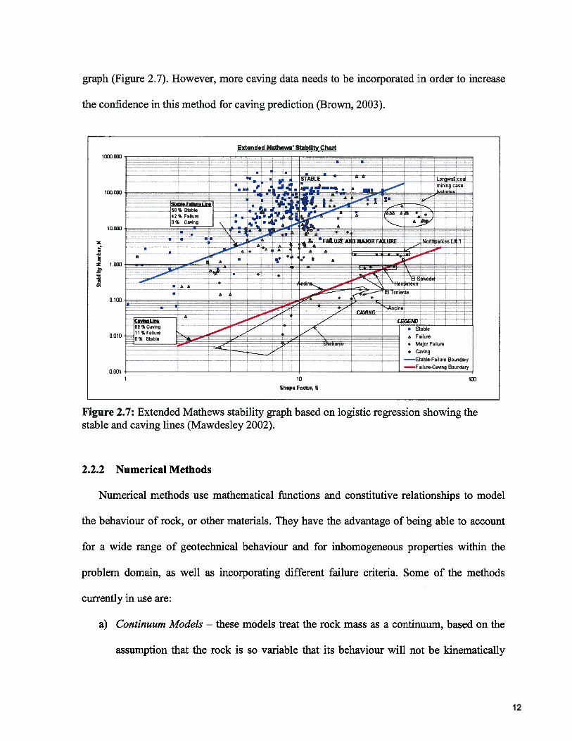
graph (Figure 2.7). However, more caving data needs to be incorporated in order to increase

the confidence in this method for caving prediction (Brown, 2003).

Figure 2.7: Extended Mathews stability graph based on logistic regression showing thestable and caving lines (Mawdesley 2002).

2.2.2 Numerical Methods

Numerical methods use mathematical functions and constitutive relationships to model

the behaviour of rock, or other materials. They have the advantage of being able to account

for a wide range of geotechnical behaviour and for inhomogeneous properties within the

problem domain, as well as incorporating different failure criteria. Some of the methods

currently in use are:

a) Continuum Models — these models treat the rock mass as a continuum, based on the

assumption that the rock is so variable that its behaviour will not be kinematically

Extended Mathews Stability Chart

z

az

ID 100

Shape Factor, S

12

controlled by specific discontinuity sets. The rock mass properties are defined as

equivalent parameters (i.e. incorporating both intact rock and joints). They assume the

material response may be described by the theories of elasticity or plasticity (Brown,

2003), represented as fiexural deformation and plastic yield. Some examples of

continuous models are: the finite difference codes FLAC (Itasca, 2005) and FLAC3D

(Itasca, 2004c); the finite element programs Phase2 (Rocsience, 2004) and Abaqus

(Simulia, 2007); and the boundary element code Map3D (Mine Modeling, 2006). The

most commonly used continuum model codes for caveability and subsidence

assessment are FLAC, FLAC3D and Abaqus. Work using FLAC and FLAC3D has

been performed by Singh et al. (1993) for Rajpura Dariba and Kiruna mines,

Karzulovic et al. (1999) for El Teniente, and Flores and Karzulovic (2003) for the

International Caving Study (conceptual models). Studies with Abaqus have been

carried out for BHP’s Nickel West and Diamond divisions by Beck et al. (2006a,

2006b). FLAC3D has been used for the pre-feasibility and feasibility caveability

assessments at Northparkes in Australia (Lift 2 and E48) and Palabora in South

Africa. Abaqus was employed for caveability assessments at Argyle Diamonds in

Australia.

b) Discontinuum Models — rock is inherently discontinuous, therefore methods that

explicitly include the presence of discontinuities present an attractive option for

caveability assessment. Discrete element methods (DEM) are more complex and

computationally intensive which makes them currently unsuitable for large scale 3D

modeling (Brown, 2003). Nevertheless, they provide an aid in understanding the

caving process. DEM codes represent rock masses in two ways: as an assembly of

13

deformable or rigid blocks subject to block movement and/or block deformation (e.g.

UDEC and 3DEC, Itasca, 2004a, b); or as an assembly of rigid bonded particles under

the influence of bond breakages and particle movements (e.g. PFC and PFC3D,

Itasca, 2008, and Rebop, Itasca, 2004d). UDEC and 3DEC have been used for

caveability assessment (Palabora), but are more commonly employed for surface

subsidence and pillar stability investigations, such as the work performed by Li and

Brummer (2005) at Palabora. Caveability studies using DEM codes are generally

carried out using PFC or PFC3D, for example, the research performed by Pierce et al.

(2007) and Reyes-Montes et al. (2007) back analyzing Northparkes’ Lift 2 cave, and

Mas Ivars et al. (2008) looking at the strain-strain response curve from synthetic rock

mass UCS tests on carbonatite material from Palabora. PFC3D was also used by

Gilbride et al. (2005) to assess subsidence at the Questa mine.

c) Hybrid Models — these models incorporate combined continuum-discontinuum

techniques providing a platform for the analysis of complex engineering problems.

One such code is ELFEN (Rockfield, 2006), which is a program developed originally

for dynamic modeling of impact loading on brittle materials, incorporating finite and

discrete element analysis techniques (Elmo et al., 2007a). The code has two

constitutive fracture models implemented: the Rarikine rotating crack model and the

Mohr-Coulomb model with a Rankine cut off (Vyazmensky et al., 2007). ELFEN has

been applied to block caving by Esci and Dutko (2003) and Pine et al. (2006)

showing promising results. More recently, Elmo at al. (2007a) and Vyazmensky et al.

(2007) have been using ELFEN to characterize surface subsidence and open-pit/block

14

cave interaction, and Rance et al. (2007) has been applying it to fragmentation

estimations.

Recent developments in numerical modeling have involved new methods of simulating

caving and surface subsidence to incorporate the pre-caving natural fracture system. Two

examples are the combinations of Synthetic Rock Mass (SRM)-DEM (Mas Ivars et al.,

2008), Finite Difference/SRM (Cundall et al., 2008; Sainsbury et al., 2008) and FEM/DEM

Discrete Fracture Network (DFN) simulations.

The SRM-DEM method consists of simulating a rock mass as an assembly of bonded

spheres with an embedded discrete network of disc-shaped joints. The three main properties

necessary for the construction of a SRM model are the intact rock properties, a discrete

fracture network and the joint properties (Pierce et al., 2007). All samples are generated in

PFC3D, where the analysis is conducted simulating the stress conditions typical of deep

block caved ore bodies (Reyes-Montes et al., 2007). The back analysis of Northparkes’ Lift 2

mine using microseismicity records (Reyes-Montes et al., 2007) and rock mass behaviour

simulation of the same mine (Pierce et a!., 2007) have been able to accurately represent what

was observed during the mine’s operation.

The FEM/DEM-DFN method also uses a synthetic rock mass, but this is developed from

DFN models in conjunction with FEM/DEM simulations to derive the rock mass properties.

This provides a link between mapped fracture systems and rock mass strength as opposed to

using empirical rock mass classifications alone (Elmo et al., 2008a). The synthetic rock mass

is used for modeling the effects of caving on the surface or in surface-underground

interactions. Elmo et al. (2008a) have reported that this method has realistically captured the

effects of block cave mining on surface subsidence. Further work is underway to incorporate

15

other variables, including in-situ rock stress, different surface geometries and undercut

drawing sequences.

Numerical models show great promise for the future as ongoing advances in computing

power and refinement of algorithms and models will allow more realistic simulation of

caving processes and caveability assessment. Nevertheless, a great deal of work needs to be

done to develop realistic geotechnical models.

2.3 Fragmentation

Fragmentation has an important impact on the overall success and profitability of block

cave operations. There are many design and operating parameters influenced by

fragmentation, including (Laubscher, 2000; Brown, 2003):

• Drawpoint size and spacing;

• Equipment selection;

• Draw control;

• Production rates;

• Dilution entry;

• Hang-ups;

• Secondary breakage;

• Staffing levels; and

• Processing plant design and costs.

Table 2.1 describes the potential effects of different fragmentation sizes on caving

operations.

Fragmentation is generally classified into three components (Laubscher, 2000; Brown, 2003):

16

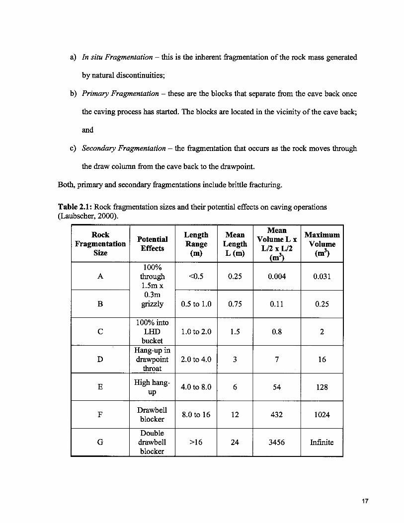
a) In situ Fragmentation — this is the inherent fragmentation of the rock mass generated

by natural discontinuities;

b) Primary Fragmentation — these are the blocks that separate from the cave back once

the caving process has started. The blocks are located in the vicinity of the cave back;

and

c) Secondary Fragmentation — the fragmentation that occurs as the rock moves through

the draw column from the cave back to the drawpoint.

Both, primary and secondary fragmentations include brittle fracturing.

Table 2.1: Rock fragmentation sizes and their potential effects on caving operations(Laubscher, 2000).

MeanRock Length Mean Maximum

Potential Volume L xFragmentation Range LengthL12 x L12

VolumeEffectsSize (m) L (m) (3) (mi)

100%A through <0.5 0.25 0.004 0.03 1

1.5mx0.3m

B grizzly 0.5 to 1.0 0.75 0.11 0.25

100% intoC LHD 1.0 to 2.0 1.5 0.8 2

bucketHang-up in

D drawpoint 2.0 to 4.0 3 7 16throat

High hangE 4.0 to 8.0 6 54 128

up

DrawbellF 8.Otol6 12 432 1024

blocker

DoubleG drawbell >16 24 3456 Infinite

blocker

17

The common measurements for block size determination are (Stille and Palmstrom,

2008):

• Rock quality designation (RQD) in drill core;

• Joint spacing in mapped surfaces, drill core or scan lines;

• Density ofjoints in mapped surfaces, drill core or scan lines; and

• Block volume in mapped surfaces.

RQD was introduced by Deere (1963) as a way of providing a quantitative estimate of

rock mass quality from drill core by measuring the percentage of core pieces longer than

10cm across the drilled core length. Grenon and Hadjigeorgiou (2003) indicated that RQD

can result in sampling bias, due to the preferential orientation of certain discontinuities. RQD

also does not account for the length of the discontinuities, and it is insensitive when the total

frequency is greater than 3m’ (moderately fractured). Moreover, RQD gives no information

about core pieces shorter than 0.lm (Palmstrom and Broch, 2006).

Palmstrom (1974) proposed the volumetric joint count (J) as a way of assessing the

amount of joints in a determined volume of rock. Volumetric joint count is defined as the

number of joints intersecting a volume of 1m3. It was modified by Palmstrom (1982) to add

an extra parameter to account for random joints:

1 1 1 1 NrJ =+++...+—+

S1 2 53 S, 5.J

where S1, S2 and S3 are average spacing for the joint sets, Nr being the number of random

joints in the actual location, and A is the area in m2. J is related to RQD using the following

equation (Palmstrom, 1974):

RQD= 115 -3.3J

18

However, it was shown by Palmstrom (2005) that RQD is very difficult to relate to other

joint measurements (such as J or block volume).

Fragmentation or block size (i.e. volume) is an important parameter in rock mechanics

and it is usually represented in the rock mass rating systems:

• In the NGI rock tunnel quality index Q (Barton et al., 1974), block size is represented

by the ratio between RQD and the joint number factor (Jn);

• The RMR system (Bieniawski, 1976) incorporates fragmentation with the RQD and

joint spacing factors;

• The Rock Mass Index (RMi) system (Palmstrom, 1996) uses the block volume (Vb)

and the number ofjoint sets (nj).

However, the representations of block volume in the Q and RMR systems is directly

affected by inherent problems with RQD which forms one component of the classification

parameters used in both rock mass rating systems (as discussed before). Other rock mass

rating systems like MRMR (Laubscher, 1990), Geological Strength Index (GSI) (Hoek et al,

2002), or the modified basic RMR (MBR) (Kendorski et al, 1982) are indirectly affected by

the RQD, since most of them are based on or use RMR as an input factor.

The RMi system directly estimates the mean block volume by using the following

equation (Palmstrom, 1996):

• ss2s3•sin sin 72 sin

where 51, S2, S3 are the mean spacing between joint sets and ‘yr, 72, ‘y are the mean acute

angles between the joint sets.

19

Cai et al. (2004) modified Palmstrom’s mean volume equation to account for impersistent

joints by adding a joint persistence factor to each fracture set, to calculate an equivalent block

volume:

V— s1s2s3

_____

b— siny1 siny2siny3Jp1p2p3

where p1 is the joint persistence factor estimated by using the following criteria:

= L l<L,

pi=l li,•

where i is the accumulated joint length of set i in the sampling plane, and L is the

characteristic length of the rock mass under consideration. Cai et al. (2004) used the

equivalent block volume and their joint condition factor as a supplementary quantitative

approach to the GSI system.

Kim et al. (2007) performed a correlation analysis relating block sizes generated with

UDEC and 3DEC against those calculated using the equivalent block volume equation,

validating the method proposed by Cai et al. (2004).

Kalenchuk et al. (2006) developed the Block Shape Characterization Method (BSCM) for

identifying the shape characteristics of individual blocks, as well as the shape distribution of

an entire rock mass. Two parameters were derived:

• The a parameter describing the shortening of the minor principal axis of the block;

and

. The 3 parameter describing the elongation of the major axis of the block.

20

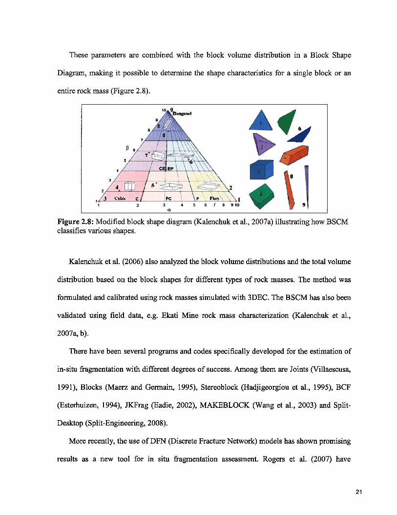
These parameters are combined with the block volume distribution in a Block Shape

Diagram, making it possible to determine the shape characteristics for a single block or an

entire rock mass (Figure 2.8).

4

Figure 2.8: Modified block shape diagram (Kalenchuk et al., 2007a) illustrating how BSCMclassifies various shapes.

Kalenchuk et al. (2006) also analyzed the block volume distributions and the total volume

distribution based on the block shapes for different types of rock masses. The method was

formulated and calibrated using rock masses simulated with 3DEC. The BSCM has also been

validated using field data, e.g. Ekati Mine rock mass characterization (Kalenchuk et al.,

2007a, b).

There have been several programs and codes specifically developed for the estimation of

in-situ fragmentation with different degrees of success. Among them are Joints (Villaescusa,

1991), Blocks (Maerz and Germain, 1995), Stereoblock (Hadjigeorgiou et al., 1995), BCF

(Esterhuizen, 1994), JKFrag (Eadie, 2002), MAKEBLOCK (Wang et al., 2003) and Split-

Desktop (Split-Engineering, 2008).

More recently, the use of DFN (Discrete Fracture Network) models has shown promising

results as a new tool for in situ fragmentation assessment. Rogers et al. (2007) have

1 2a

4 5 6 6 910

21

demonstrated that DFN modeling clearly has application in the estimation of fragmentation.

Elmo et al. (2008b) have characterized fragmentation through DFN models and have related

them to Cai et al.’s (2004) work with GSI. The DFN has also been used for defining fracture

networks in synthetic rock masses (Pierce et al., 2007), together with hybrid codes (ELFEN)

(Rance et al., 2007) to estimate fragmentation.

2.4 The Discrete Fracture Network (DFN)

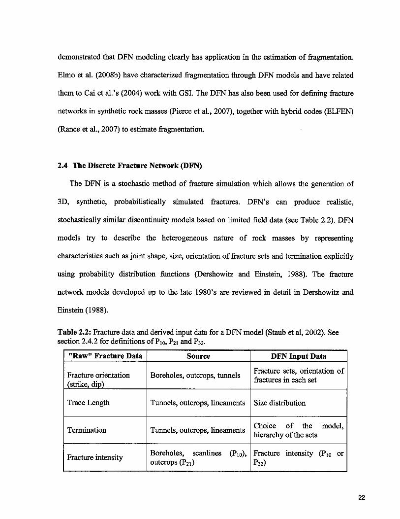
The DFN is a stochastic method of fracture simulation which allows the generation of

3D, synthetic, probabilistically simulated fractures. DFN’s can produce realistic,

stochastically similar discontinuity models based on limited field data (see Table 2.2). DFN

models try to describe the heterogeneous nature of rock masses by representing

characteristics such as joint shape, size, orientation of fracture sets and termination explicitly

using probability distribution functions (Dershowitz and Einstein, 1988). The fracture

network models developed up to the late 1980’s are reviewed in detail in Dershowitz and

Einstein (1988).

Table 2.2: Fracture data and derived input data for a DFN model (Staub et al, 2002). Seesection 2.4.2 for definitions ofP10,P21 and P32.

“Raw” Fracture Data Source DFN Input Data

Fracture sets, orientation ofFracture orientation Boreholes, outcrops, tunnelsfractures in each set(strike, dip)

Trace Length Tunnels, outcrops, lineaments Size distribution

Choice of the model,Termination Tunnels, outcrops, lineamentshierarchy of the sets

Boreholes, scanlines (P10), Fracture intensity (P10 orFracture intensityoutcrops (P21) P32)

22

Since its conception, the DFN method has been continuously developed, with many

applications in civil, environmental and reservoir engineering (Jing, 2003). The method first

saw use in characterization of the permeability of fractured rock masses and generic studies

on fracture properties. Some examples are the work of Layton et al. (1992) and Watanabe

and Takahashi (1995) on hot-dry-rock reservoirs; Dershowitz (1992) on characterization of

the permeability of fractured rocks; and Rouleau and Gale (1987) on water effects on

underground excavations in rock. DFN modeling has been used in the oil and gas industry

for the simulation of hydrocarbon reservoirs (Dershowitz et al., 1998a) and in the nuclear

industry for the modeling of nuclear waste repositories. It has also been identified as a useful

tool for dealing with geomechanical problems in rock. A few examples are: Starzec and

Tsang (2002) looking at the stability of tunnels; Grenon and Hadjigeorgiou (2003) studying

open stope stability; Rogers et al. (2007) and Elmo et al. (2008b) analyzing fragmentation of

fractured rock; Vyazmensky et al. (2008) using DFNs as input for hybrid brittle fracture

models in the analysis of progressive rock slope failure in response to underground block

cave mining; and Hadjigeorgiou et al. (2008) analysing the stability of vertical excavations in

hard rock by integrating a DFN system into a PFC model.

2.4.1 Fracture Size

Fracture size or persistence is one of the critical factors establishing the formation and

size of 3D blocks or incomplete blocks in a rock mass (Rogers et al., 2007), as well as having

a significant influence on the rock mass properties. Fracture length is often a critical input in

DFN models and a key parameter for sensitivity studies (Rogers et al., 2006).

23

It is almost impossible to determine persistence without taking apart the rock volume

being studied and measuring it directly. Therefore, the length of the rock discontinuities must

be inferred from the data sampled at outcrops, rock cuts or tunnel faces. This information at

the same time suffers from statistical biases generated at several levels. Zhang and Einstein

(1998) attributed these sampling errors to four different type of bias:

1. Orientation bias: the probability of a joint appearing in an outcrop depends on the

relative orientation between the outcrop and the joint;

2. Size bias: large joints are more likely to be sampled than small joints. This bias

results in two ways: a) a larger joint is more likely to appear in an outcrop than a

smaller one; and b) a longer trace is more likely to appear in a sampling area than a

shorter one;

3. Truncation bias: very small trace lengths are difficult or sometimes impossible to

measure. Therefore, trace lengths below some known cut-off length are not recorded;

and

4. Censoring bias: long joint traces may extend beyond the visible exposure so that one

end or both ends of the joint traces cannot be seen (Figure 2.9).

24

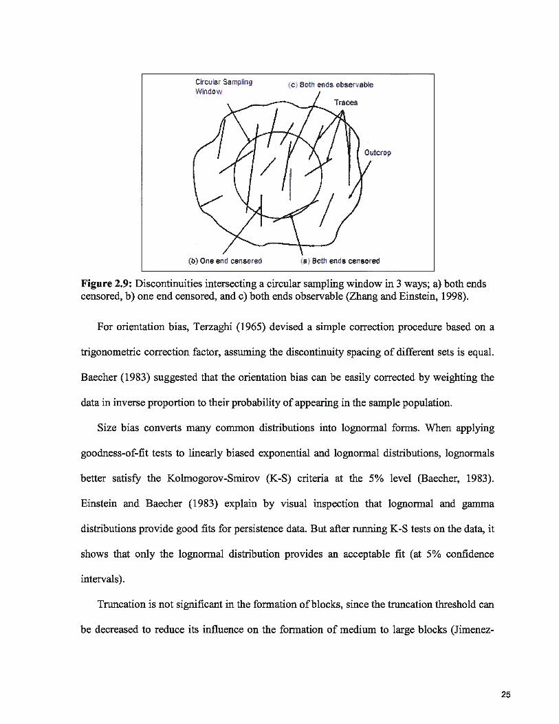
Figure 2.9: Discontinuities intersecting a circular sampling window in 3 ways; a) both endscensored, b) one end censored, and c) both ends observable (Zhang and Einstein, 1998).

For orientation bias, Terzaghi (1965) devised a simple correction procedure based on a

trigonometric correction factor, assuming the discontinuity spacing of different sets is equal.

Baecher (1983) suggested that the orientation bias can be easily corrected by weighting the

data in inverse proportion to their probability of appearing in the sample population.

Size bias converts many common distributions into lognormal fonns. When applying

goodness-of-fit tests to linearly biased exponential and lognorinal distributions, lognormals

better satisfy the Kolmogorov-Smirov (K-S) criteria at the 5% level (Baecher, 1983).

Einstein and Baecher (1983) explain by visual inspection that lognormal and gamma

distributions provide good fits for persistence data. But after running K-S tests on the data, it

shows that only the lognormal distribution provides an acceptable fit (at 5% confidence

intervals).

Truncation is not significant in the formation of blocks, since the truncation threshold can

be decreased to reduce its influence on the formation of medium to large blocks (Jimenez

Circu’ar SarnpiirTçWin cc w

9c: enri cbserable

races

C utcrc p

(b) One end censc red ‘a) 5cth ends censcred

25

Rodriguez and Sitar, 2006). According to Baecher (1983), truncation may be safely ignored

in most cases if the truncation level is small compared to the problem scale.

Censoring bias is a very significant issue. This bias is more likely to adversely affect the

analysis of the rock mass, since it occurs with proportionally higher probability for longer

traces. This causes the samples to be biased towards shorter lengths (Baecher, 1983),

potentially affecting the generation of large blocks in the model. Mauldon (1998) developed

a method for overcoming this bias by using density and mean trace length estimators. Zhang

and Einstein (2000) also proposed a method for obtaining the true trace length distribution

for circular windows.

In the future, laser scanning (LiDAR) and digital photogrametry technology may provide

another source of information for fracture length assessment. These systems might even help

overcome some of the sample biases (e.g. truncation bias). They also allow the measurement

of large exposed faces that have difficult or limited access.

2.4.2 Fracture Density and Spacing

Fracture density is defined as the mean number of trace centers per unit area (Mauldon,

1998). Discontinuities in a rock mass can only be characterized in a finite volume of rock.

This information is generally obtained through boreholes, or through outcrop mapping and

scanlines.

Data gathered using boreholes and scanlines is considered to be one-dimensional and is

usually denoted as fracture frequency. In DFN terminology, this parameter is defined a P10

(m’), which is the fracture frequency along a scanline or borehole.

26

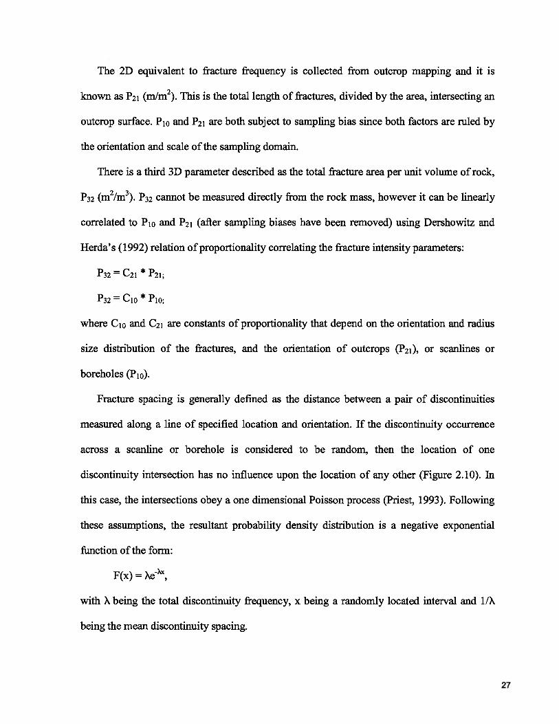
The 2D equivalent to fracture frequency is collected from outcrop mapping and it is

known as P21 (mJm2). This is the total length of fractures, divided by the area, intersecting an

outcrop surface. P10 and P21 are both subject to sampling bias since both factors are ruled by

the orientation and scale of the sampling domain.

There is a third 3D parameter described as the total fracture area per unit volume of rock,

P32 (m2/m3).P32 cannot be measured directly from the rock mass, however it can be linearly

correlated to P10 and P21 (after sampling biases have been removed) using Dershowitz and

Herda’ s (1992) relation of proportionality correlating the fracture intensity parameters:

P32 = C21 * P21;

P32 C10 * P10;

where C10 and C21 are constants of proportionality that depend on the orientation and radius

size distribution of the fractures, and the orientation of outcrops (P21), or scanlines or

boreholes (P10).

Fracture spacing is generally defined as the distance between a pair of discontinuities

measured along a line of specified location and orientation. If the discontinuity occurrence

across a scanline or borehole is considered to be random, then the location of one

discontinuity intersection has no influence upon the location of any other (Figure 2.10). In

this case, the intersections obey a one dimensional Poisson process (Priest, 1993). Following

these assumptions, the resultant probability density distribution is a negative exponential

function of the form:

F(x) = Xe,

with X being the total discontinuity frequency, x being a randomly located interval and 1/X

being the mean discontinuity spacing.

27

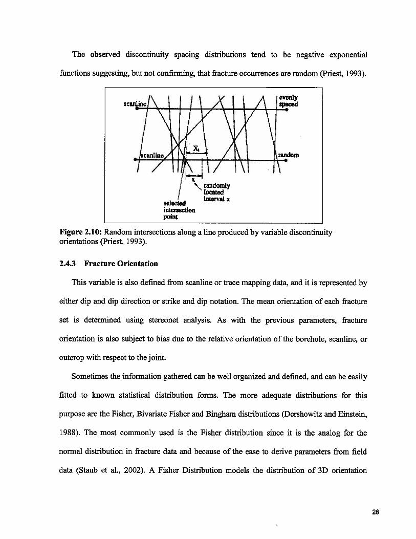
The observed discontinuity spacing distributions tend to be negative exponential

functions suggesting, but not confirming, that fracture occurrences are random (Priest, 1993).

Figure 2.10: Random intersections along a line produced by variable discontinuityorientations (Priest, 1993).

2.4.3 Fracture Orientation

This variable is also defined from scanline or trace mapping data, and it is represented by

either dip and dip direction or strike and dip notation. The mean orientation of each fracture

set is determined using stereonet analysis. As with the previous parameters, fracture

orientation is also subject to bias due to the relative orientation of the borehole, scanline, or

outcrop with respect to the joint.

Sometimes the information gathered can be well organized and defined, and can be easily

fitted to known statistical distribution forms. The more adequate distributions for this

purpose are the Fisher, Bivariate Fisher and Bingham distributions (Dershowitz and Einstein,

1988). The most commonly used is the Fisher distribution since it is the analog for the

normal distribution in fracture data and because of the ease to derive parameters from field

data (Staub et al., 2002). A Fisher Distribution models the distribution of 3D orientation

intersectIøpoint

28

vectors, like the distribution of joint orientations (pole vectors) on a sphere (Fisher, 1953).

The Fisher Distribution describes the angular distribution of orientations about a mean

orientation vector, and is symmetric about the mean. The probability density function can be

expressed as:

f(O)=

e” _e_C

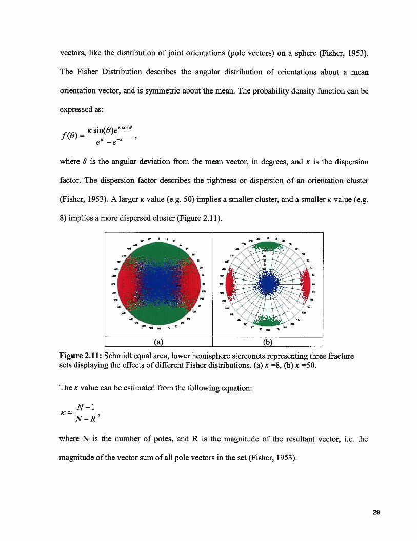
where 0 is the angular deviation from the mean vector, in degrees, and K is the dispersion

factor. The dispersion factor describes the tightness or dispersion of an orientation cluster

(Fisher, 1953). A larger K value (e.g. 50) implies a smaller cluster, and a smaller K value (e.g.

8) implies a more dispersed cluster (Figure 2.11).

(b)

Figure 2.11: Schmidt equal area, lower hemisphere stereonets representing three fracturesets displaying the effects of different Fisher distributions. (a) K =8, (b) K =50.

The K value can be estimated from the following equation:

N-i

N-R

where N is the number of poles, and R is the magnitude of the resultant vector, i.e. the

magnitude of the vector sum of all pole vectors in the set (Fisher, 1953).

0 ro

70

lb

‘70

(a)

l i ITO

29

2.4.4 Fracture Spatial Model

Several conceptual models to describe the spatial distribution of discontinuities have been

developed. There are three different types of distributions employed to describe the spatial

distribution of fractures: i) considering that the fractures are ubiquitous (i.e. random in space

following a Poisson distribution); ii) clumped or clustered around a certain feature, e.g. a

fault; iii) close to constant fracturing, like in layered systems such as sedimentary rocks,

where spacing is strongly related to bed thickness (Staub et al., 2002; Rogers et al., 2007).

Most of these share common characteristics, such as size, termination and shape of fractures.

Among the models used for ubiquitous fractures is the Enhanced Baecher model. As in

the conventional Baecher model (Baecher et al., 1978), the fracture centers are located

uniformly in space using a Poisson process. The Enhanced Baecher model however, depicts

fractures as polygons with a given radius and location, and not as disks (Staub et al., 2002). It

also allows for the fracture termination to be specified.

The Nearest Neighbour model is generally utilized to simulate fractures clustered around

some major feature (for example a fault) by producing new discontinuities near earlier

fractures (Dershowitz et al., 1998a). The model organizes fractures into primary, secondary

and tertiary groups and it generates them in that sequence. The Nearest Neighbour model is

identical to the Enhanced Baecher model except for its assumptions regarding the spatial

distribution (Staub et al., 2002).

The Levy-Lee Fractal model is a commonly used model to represent layered systems. It

accounts for the chronology of fracture formation, since centers are created sequentially by

the Levy flight process in 3D. The size of the fracture is related to the distance from the

previous fracture, and fracturing can be bounded with spacing controlled by bed thickness

30

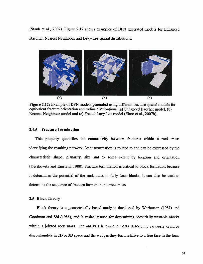
(Staub et al., 2002). Figure 2.12 shows examples of DFN generated models for Enhanced

Baecher, Nearest Neighbour and Levy-Lee spatial distributions.

Figure 2.12: Example of DFN models generated using different fracture spatial models forequivalent fracture orientation and radius distributions. (a) Enhanced Baecher model, (b)Nearest-Neighbour model and (c) Fractal Levy-Lee model (Elmo et al., 200Th).

2.4.5 Fracture Termination

This property quantifies the connectivity between fractures within a rock mass

identifying the resulting network. Joint termination is related to and can be expressed by the

characteristic shape, planarity, size and to some extent by location and orientation

(Dershowitz and Einstein, 1988). Fracture termination is critical to block formation because

it determines the potential of the rock mass to fully form blocks. It can also be used to

determine the sequence of fracture formation in a rock mass.

2.5 Block Theory

Block theory is a geometrically based analysis developed by Warburton (1981) and

Goodman and Shi (1985), and is typically used for determining potentially unstable blocks

within a jointed rock mass. The analysis is based on data describing variously oriented

discontinuities in 2D or 3D space and the wedges they form relative to a free face in the form

31

of an underground excavation (Goodman, 1995). This makes block theory useful for the

analysis of blocks that separate from the cave back once the caving process has started

(primary fragmentation). The theory divides blocks into removable and non removable.

Removable blocks are finite and kinematically free to fall or slide. The latter involves a

stability check under the applied forces (generally block weight and ffiction). Blocks which

are unstable (i.e. factor of safety less than one) and removable are the “key blocks” of the

excavation. Blocks that are stable (factor of safety greater than 1; i.e. friction preventing

sliding) and removable are called “potential key blocks”. There is a third category called

“safe removable blocks” which are blocks that are removable, but their face orientations

prevent them from moving (Table 2.3).

32

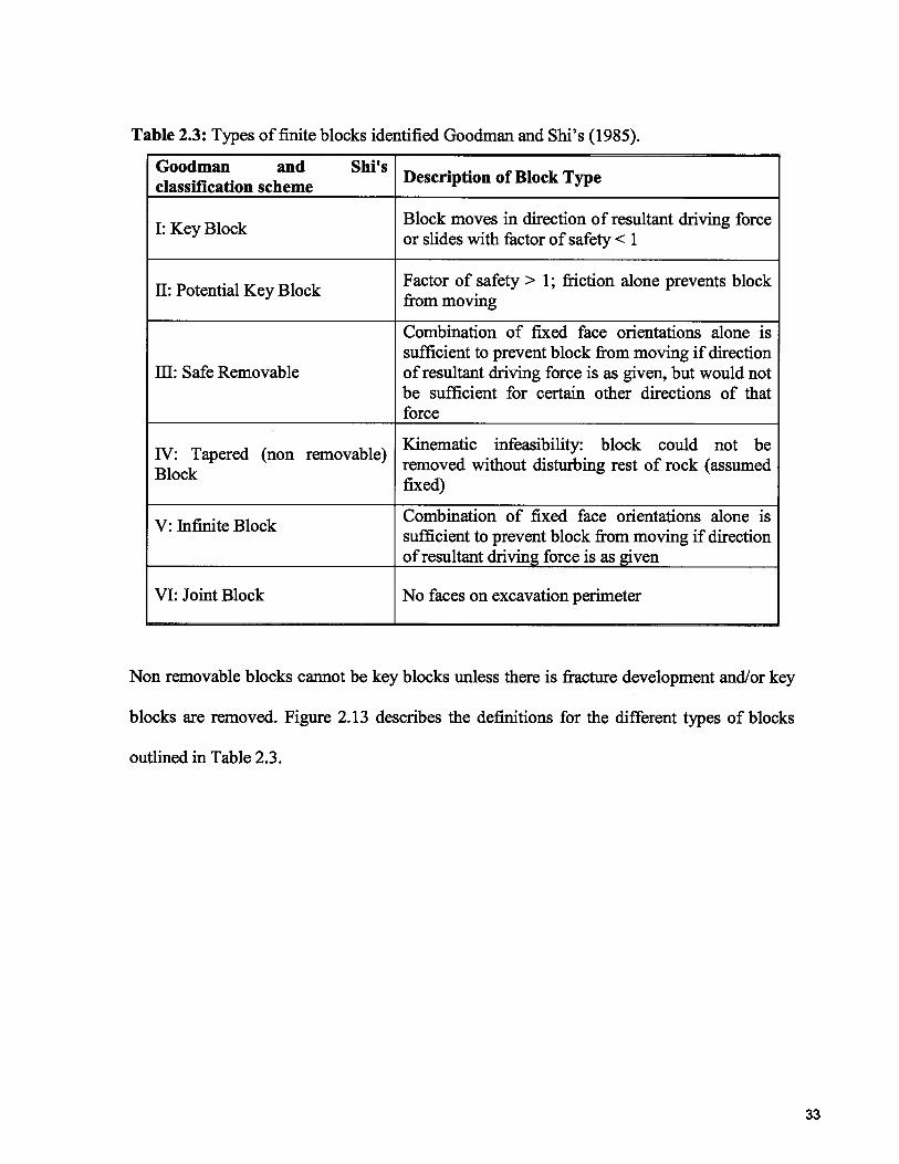
Table 2.3: Types of finite blocks identified Goodman and Shi’s (1985).

Goodman and Shi’sclassification scheme

Description of Block Type

Block moves in direction of resultant driving forceI: Key Blockor slides with factor of safety < 1

Factor of safety> 1; friction alone prevents blockII: Potential Key Blockfrom moving

Combination of fixed face orientations alone issufficient to prevent block from moving if direction

III: Safe Removable of resultant driving force is as given, but would notbe sufficient for certain other directions of thatforce

Kinematic infeasibility: block could not beIV: Tapered (non removable)removed without disturbing rest of rock (assumedBlockfixed)

Combination of fixed face orientations alone isV: Infinite Block

sufficient to prevent block from moving if directionof resultant driving force is as given

VI: Joint Block No faces on excavation perimeter

Non removable blocks cannot be key blocks unless there is fracture development and/or key

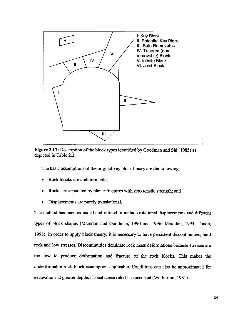
blocks are removed. Figure 2.13 describes the definitions for the different types of blocks

outlined in Table 2.3.

33

/

Figure 2.13: Description of the block types identified by Goodman and Shi (1985) asdepicted in Table 2.3.

The basic assumptions of the original key block theory are the following:

• Rock blocks are undeformable;

• Rocks are separated by planar fractures with zero tensile strength; and

• Displacements are purely translational.

The method has been extended and refined to include rotational displacements and different

types of block shapes (Mauldon and Goodman, 1990 and 1996; Mauldon, 1995; Tonon,

1998). Tn order to apply block theory, it is necessary to have persistent discontinuities, hard

rock and low stresses. Discontinuities dominate rock mass deformations because stresses are

too low to produce deformation and fracture of the rock blocks. This makes the

underformable rock block assumption applicable. Conditions can also be approximated for

excavations at greater depths if local stress relief has occurred (Warburton, 1981).

I: Key BlockII: Potential Key BlockIll: Safe RemovableIV: Tapered (nonremovable) BlockV: Infinite BlockVI: Joint Block

‘4

34

Block stability analysis with block theory is conducted either analytically by vector

techniques, or graphically using stereographic projections. Block theory is based on the idea

that a single plane divides the three dimensional space into upper and lower half space.

Goodman and Shi (1985) use “0” to indicate the upper half space and “1” for the lower half

space and a string to represent a block formed. For instance, the string 101 represents a block

formed by three joints relative to an excavation face, which include: the lower side of joint

set one, the upper side of joint set two and the lower side of joint set three. The theory

translates each of the discontinuities and free faces so that they each pass through a common

origin forming a series of pyramids:

• Block Pyramid — assemblage of planes forming a particular set of blocks;

• Joint Pyramid — group of discontinuity planes (rock to rock interfaces);

• Excavation Pyramid — group of excavation surfaces (rock to air interfaces).

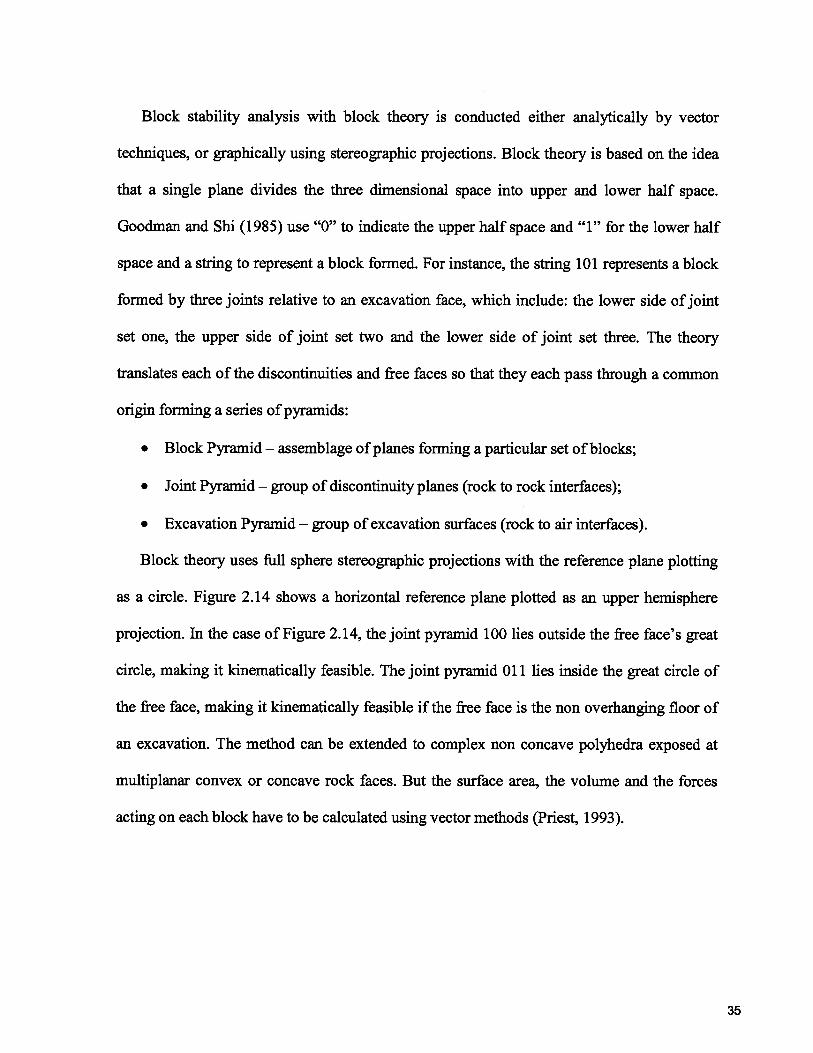
Block theory uses full sphere stereographic projections with the reference plane plotting

as a circle. Figure 2.14 shows a horizontal reference plane plotted as an upper hemisphere

projection. In the case of Figure 2.14, the joint pyramid 100 lies outside the free face’s great

circle, making it kinematically feasible. The joint pyramid 011 lies inside the great circle of

the free face, making it kinematically feasible if the free face is the non overhanging floor of

an excavation. The method can be extended to complex non concave polyhedra exposed at

multiplanar convex or concave rock faces. But the surface area, the volume and the forces

acting on each block have to be calculated using vector methods (Priest, 1993).

35

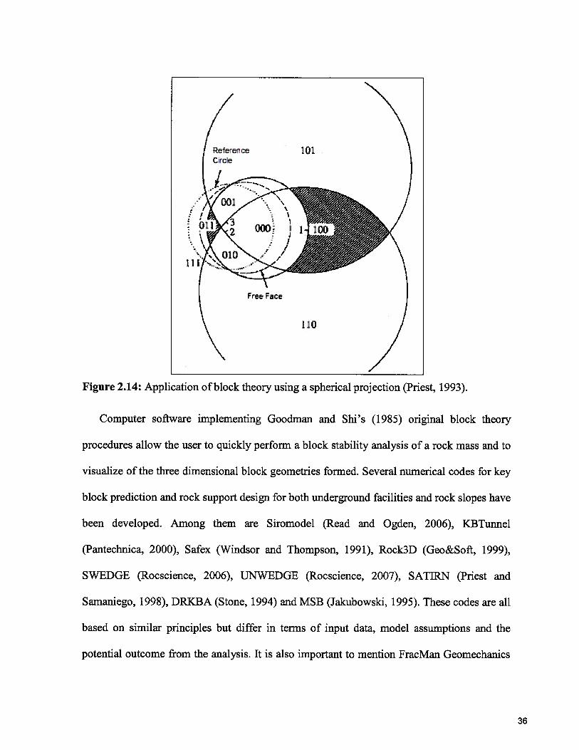
Figure 2.14: Application ofblock theory using a spherical projection (Priest, 1993).

Computer software implementing Goodman and Shi’s (1985) original block theory

procedures allow the user to quickly perform a block stability analysis of a rock mass and to

visualize of the three dimensional block geometries formed. Several numerical codes for key

block prediction and rock support design for both underground facilities and rock slopes have

been developed. Among them are Siromodel (Read and Ogden, 2006), KBTunnel

(Pantechnica, 2000), Safex (Windsor and Thompson, 1991), Rock3D (Geo&Soft, 1999),

SWEDGE (Rocscience, 2006), UNWEDGE (Rocscience, 2007), SATIRN (Priest and

Samaniego, 1998), DRKBA (Stone, 1994) and MSB (Jakubowski, 1995). These codes are all

based on similar principles but differ in terms of input data, model assumptions and the

potential outcome from the analysis. It is also important to mention FracMan Geomechanics

Reference 101Circle

/ 001

Free Face

110 II

36

(Golder Associates, 2007; Dershowitz et al., 1998b) which combines DFN simulation with

block theory, in order to evaluate the stability of underground openings.

The procedures used by UNWEDGE to calculate the stability of a rock block follows a

similar algorithm as FracMan Geomechanics. UNWEDGE determines all the possible

wedges which can be formed with at least three distinct joint planes and an excavation face

(Figure 2.15). In general, most of the wedges formed with UNWEDGE are tetrahedral in

nature, but prismatic wedges can also be formed.

Once the program determines the wedge coordinates, it calculates the geometrical

properties of each wedge including: wedge volume, wedge face areas and normal vectors for

each plane. The forces on the wedge are classified as active or passive. Active forces involve

the driving forces in the factor of safety calculation (e.g. wedge weight) and passive forces

involving the resisting forces (e.g. support resistance). The individual force vectors are

computed for magnitude and then the resultant active and passive force vectors are

determined by vector summation of the individual forces (Rocscience, 2003). Once the

program computes the wedge geometry, it calculates the sliding direction based on Goodman

AA

Figure 2.15: Example of tunnel stability analysis performed with UNWEDGE (Rocscience,2007).

37

and Shi’s (1985) method. After the sliding direction has been determined, the normal forces

to the planes are calculated which is followed by the shear and tensile strength computation

(using either the Mohr-Coulomb, the Barton-Bandis or the Power Curve criterion). When all

the forces are computed, the resultant factor of safety is determined (Rocscience, 2003).

Another approach to block stability is taken with the use of implicit DEM modeling, for

example discontinuous deformation analysis (DDA) and distinct element modeling (e.g.

IJDEC). DDA can represent motion and deformation of the individual bodies by using an

implicit solution with finite element discretization of the body interior (Jing and Stephansson,

2007). This is likewise done in UDEC (Cundall and Hart, 1993) and 3DEC by discretizing all

the blocks to overcome the condition of undeformable blocks.

2.6 Chapter Summary

Block caving is an underground mining method that has been gaining importance because

of its low costs and high production rates.

In order to assess the caveability of an ore body, two different methods are generally

employed: empirical and numerical. Empirical methods are based on experiences in a large

number of mines and numerical methods use mathematical algorithms to simulate the

behaviour of rock. In the last few years, numerical methods have shown significant algorithm

improvements, which has been accompanied by an increase in computing power.

Fragmentation also plays a major role in block caving, particularly when it comes to the

design and logistics of a mine.

The DFN is a stochastic method of fracture simulation which allows the generation of

simulated fractures. It can produce realistic, stochastically similar discontinuity models based

38

on limited field data, describing the heterogeneous nature of rock masses by representing

characteristics such as joint shape, size, orientation of fracture sets and termination explicitly

using probability distribution functions.

Block theory is a geometrically based analysis used for determining potentially unstable

blocks within a jointed rock mass. The analysis is based on data describing variously oriented

discontinuities in 2D or 3D space, and the wedges they form relative to a free face in the

form of an underground excavation or a slope.

Computer codes have been developed that combine both DFN simulation and the

principles of block theory to assess the stability of underground openings. FracMan

Geomechanics is one such programs and will be extensively used in this thesis.

39

3.0 METHODOLOGY

The discrete fracture network models simulated in this research were generated using the

proprietary code FracMan Geomechanics (Golder Associates, 2007; Dershowitz et al.,

1998b).

3.1 Characteristics of the Model

FracMan allows the user to choose a range of values and/or different models for fracture

spatial distribution, fracture orientation and orientation distribution, fracture termination

percentage, fracture radius distribution, and fracture intensity in order to simulate the

conditions present in a given rock mass. After generating a DFN stochastic model from the

assumed parameters, FracMan identifies the 3D blocks that have a common face with the

opening being analyzed. In order to do this, the code computes the fracture intersections with

the opening, iteratively defining trace maps for all the intersections until all discontinuities

involved have a trace map of their own. After it identifies valid blocks that have formed, the

code computes their volume based on a 3D process that builds the blocks by putting together

the defined trace maps with no overlaps and no gaps (3D tessellation process). FracMan then

carries out a stability analysis checking each block for unconditional stability, free fall or

sliding (on one or two planes). The factor of safety for each block is assigned based on limit

equilibrium assumptions (Rogers et al, 2006). As mentioned in chapter 3.5, the block

stability analysis in FracMan is very similar to the one performed by UNWEDGE, utilizing

Goodman and Shi’s (1985) block theory. TJNWEDGE inputs the various combinations of

assigned joint sets, looks for potential wedges and their factor of safety. FracMan generates a

fracture network using a stochastic approach and identifies all blocks, determining their

40

factor of safety. The factor of safety (FS) is determined depending on the failure mode of a

block. Stable blocks have an infinite factor of safety and free falling blocks have a factor of

safety of zero. Between these two extremes are the cases of translational sliding on one- or

two-planes. The factor of safety for these two cases can be calculated using either the Mohr

Coulomb or the Barton—Bandis criterion (Rogers et aL, 2006). The Mohr-Coulomb model is

shown below. For sliding on a single plane, the Mohr-Coulomb criterion:

A.c+jN.tanq5FS=

Swhere A is the area of the face, c is the cohesion parameter, N’ is the normal force to the

face, is the friction angle and S is the magnitude of the shear force. For sliding on two

planes using the Mohr-Coulomb criterion:

FS—A1 c1 +N’1tançb1+A2 •c2

S12

where N’1 and N’2 are the normal forces to faces 1 and 2 respectively, A1 and A2 are the

areas of faces 1 and 2 respectively, S12 is the shear force along the edge created by faces 1

and 2, c is the cohesion parameter of face i and , is the friction angle of face i.

The DFN provides the possibility of generating multiple statistically equivalent

realizations that allow the understanding of the frequency of occurrence for blocks of a

particular size or factor of safety (Rogers et al, 2006). Figure 3.1 compares the UNWEDGE

and FracMan stability analysis for a tunnel section with the same dimensions and joint sets. It

can be observed how FracMan’s probabilistic approach is able to better characterize the

potential blocks that can form in the tunnel walls.

41

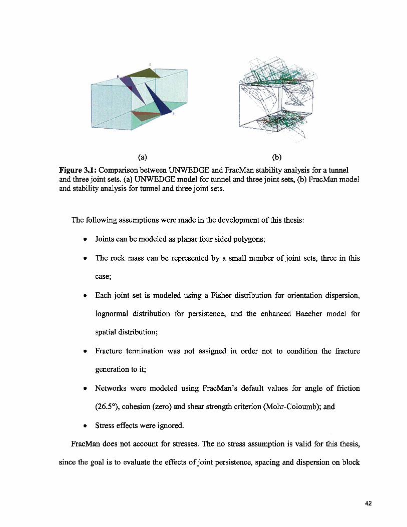
(a)

Figure 3.1: Comparison between IJNWEDGE and FracMan stability analysis for a tunneland three joint sets. (a) TINWEDGE model for tunnel and three joint sets, (b) FracMan modeland stability analysis for tunnel and three joint sets.

The following assumptions were made in the development of this thesis:

• Joints can be modeled as planar four sided polygons;

• The rock mass can be represented by a small number of joint sets, three in this

case;

• Each joint set is modeled using a Fisher distribution for orientation dispersion,

lognormal distribution for persistence, and the enhanced Baecher model for

spatial distribution;

• Fracture termination was not assigned in order not to condition the fracture

generation to it;

• Networks were modeled using FracMan’s default values for angle of friction

(26.5°), cohesion (zero) and shear strength criterion (Mohr-Coloumb); and

• Stress effects were ignored.

FracMan does not account for stresses. The no stress assumption is valid for this thesis,

since the goal is to evaluate the effects of joint persistence, spacing and dispersion on block

(b)

42

stability without the influence of brittle failure, the increase of FS due to increased shear

strength, and the clamping and “pop out” effect on wedges.

3.2 Model Geometry

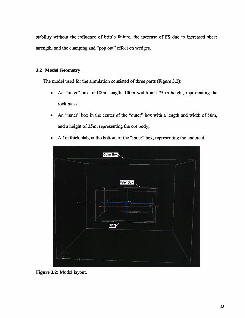
The model used for the simulation consisted of three parts (Figure 3.2):

• An “outer” box of lOOm length, lOOm width and 75 m height, representing the

rock mass;

• An “inner” box in the center of the “outer” box with a length and width of 50m,

and a height of 25m, representing the ore body;

• A 1 m thick slab, at the bottom of the “inner” box, representing the undercut.

Figure 3.2: Model layout.

43

To condition the model to a given P10 value, three orthogonal boreholes passing through

the center of each of the boxes were inserted.

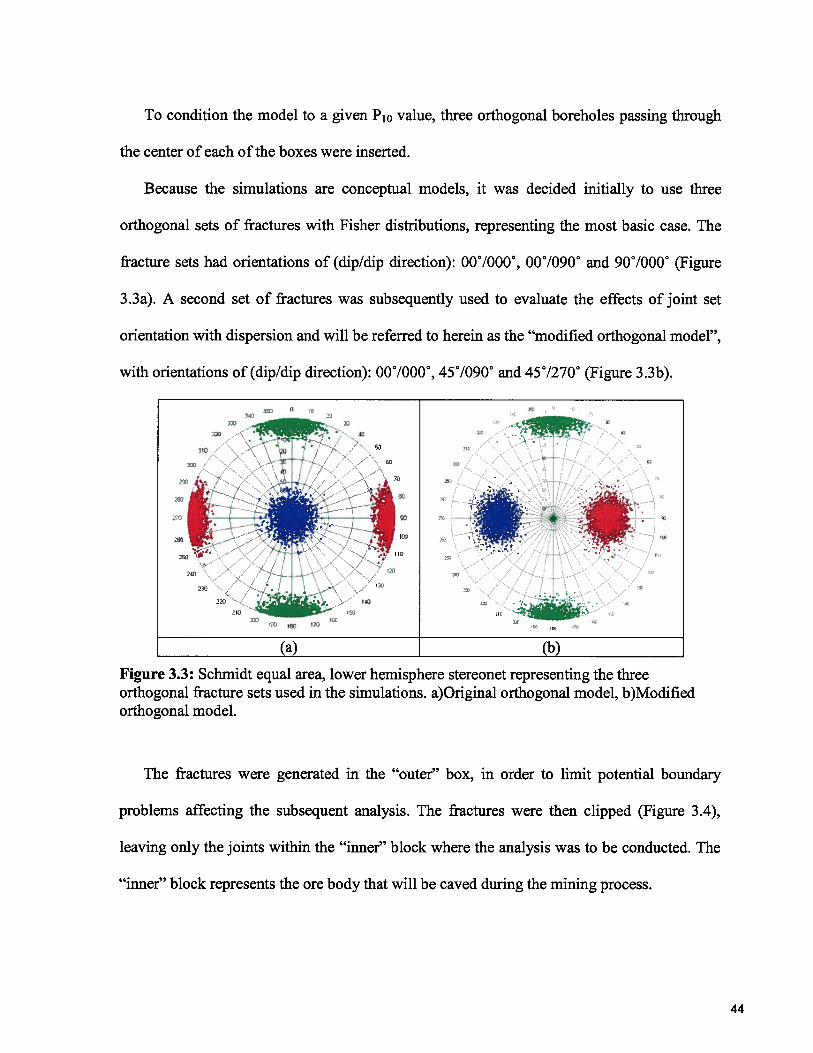
Because the simulations are conceptual models, it was decided initially to use three

orthogonal sets of fractures with Fisher distributions, representing the most basic case. The

fracture sets had orientations of (dip/dip direction): 000/0000, 000/0900 and 900/0000 (Figure

3.3 a). A second set of fractures was subsequently used to evaluate the effects of joint set

orientation with dispersion and will be referred to herein as the “modified orthogonal model”,

with orientations of (dip/dip direction): 000/0000, 450/0900 and 450/2700 (Figure 3.3b).

(a) (b)

Figure 3.3: Schmidt equal area, lower hemisphere stereonet representing the threeorthogonal fracture sets used in the simulations. a)Original orthogonal model, b)Modifiedorthogonal model.

The fractures were generated in the “outer” box, in order to limit potential boundary

problems affecting the subsequent analysis. The fractures were then clipped (Figure 3.4),

leaving only the joints within the “inner” block where the analysis was to be conducted. The

“inner” block represents the ore body that will be caved during the mining process.

44

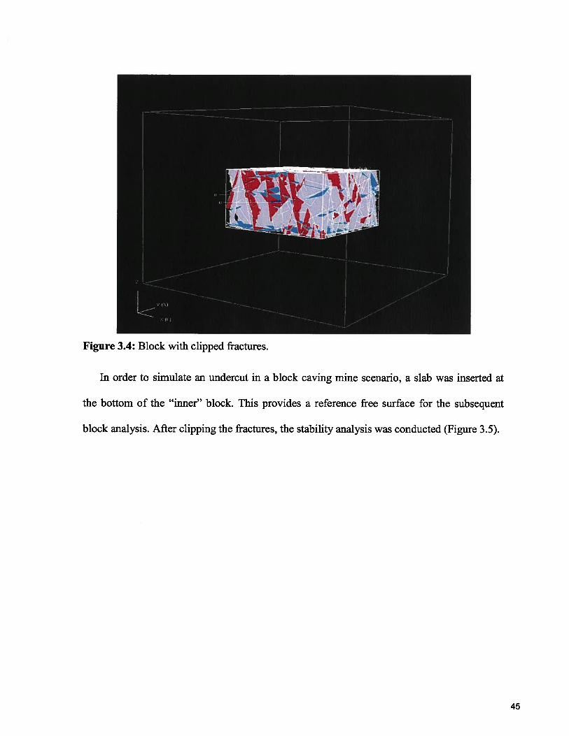
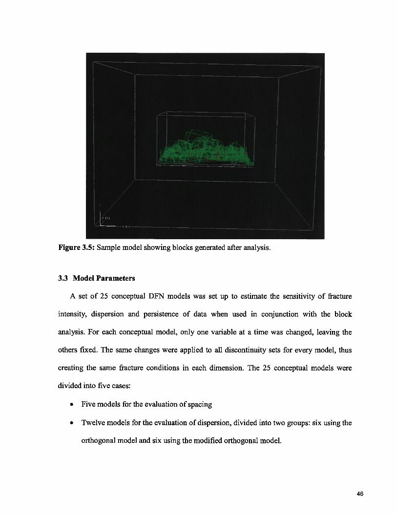
lii order to simulate an undercut in a block caving mine scenario, a slab was inserted at

the bottom of the “inner” block. This provides a reference free surface for the subsequent

block analysis. After clipping the fractures, the stability analysis was conducted (Figure 3.5).

Figure 3.4: Block with clipped fractures.

45

3.3 Model Parameters

A set of 25 conceptual DFN models was set up to estimate the sensitivity of fracture

intensity, dispersion and persistence of data when used in conjunction with the block

analysis. For each conceptual model, oniy one variable at a time was changed, leaving the

others fixed. The same changes were applied to all discontinuity sets for every model, thus

creating the same fracture conditions in each dimension. The 25 conceptual models were

divided into five cases:

• Five models for the evaluation of spacing

• Twelve models for the evaluation of dispersion, divided into two groups: six using the

orthogonal model and six using the modified orthogonal model.

Figure 3.5: Sample model showing blocks generated after analysis.

46

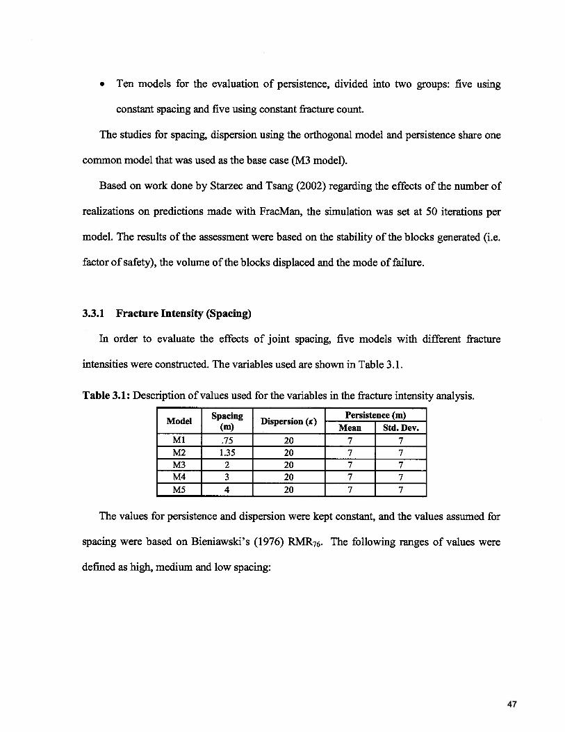
• Ten models for the evaluation of persistence, divided into two groups: five using

constant spacing and five using constant fracture count.

The studies for spacing, dispersion using the orthogonal model and persistence share one

common model that was used as the base case (M3 model).

Based on work done by Starzec and Tsang (2002) regarding the effects of the number of

realizations on predictions made with FracMan, the simulation was set at 50 iterations per

model. The results of the assessment were based on the stability of the blocks generated (i.e.

factor of safety), the volume of the blocks displaced and the mode of failure.

3.3.1 Fracture Intensity (Spacing)

In order to evaluate the effects of joint spacing, five models with different fracture

intensities were constructed. The variables used are shown in Table 3.1.

Table 3.1: Description of values used for the variables in the fracture intensity analysis.

Spacing Persistence (m)Model Dispersion (K)

(m) Mean Std. Dcv.Ml .75 20 7 7M2 1.35 20 7 7M3 2 20 7 7M4 3 20 7 7M5 4 20 7 7

The values for persistence and dispersion were kept constant, and the values assumed for

spacing were based on Bieniawski’s (1976) RMR76. The following ranges of values were

defined as high, medium and low spacing:

47

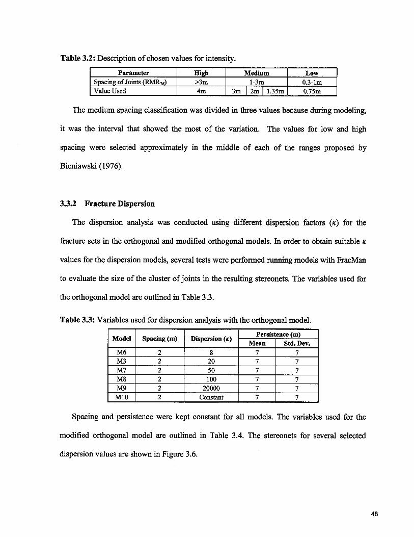
Table 3.2: Description of chosen values for intensity.

I Parameter High Medium Lowpcing of Joints (RMR76) >3m 1-3m 0.3-lm

I Value Used 4m 3m 2m 1.35m 0.75m

The medium spacing classification was divided in three values because during modeling,

it was the interval that showed the most of the variation. The values for low and high

spacing were selected approximately in the middle of each of the ranges proposed by

Bieniawski (1976).

3.3.2 Fracture Dispersion

The dispersion analysis was conducted using different dispersion factors (K) for the

fracture sets in the orthogonal and modified orthogonal models. In order to obtain suitable K

values for the dispersion models, several tests were performed running models with FracMan

to evaluate the size of the cluster of joints in the resulting stereonets. The variables used for

the orthogonal model are outlined in Table 3.3.

Model Spacing (m) Dispersion (,) Persistence (m)Mean Std. Dev.

M6 2 8 7 7M3 2 20 7 7M7 2 50 7 7M8 2 100 7 7M9 2 20000 7 7M10 2 Constant 7 7

Spacing and persistence were kept constant for all

modified orthogonal model are outlined in Table 3.4.

dispersion values are shown in Figure 3.6.

Table 3.3: Variables used for dispersion analysis with the orthogonal model.

models. The variables used for the

The stereonets for several selected

48

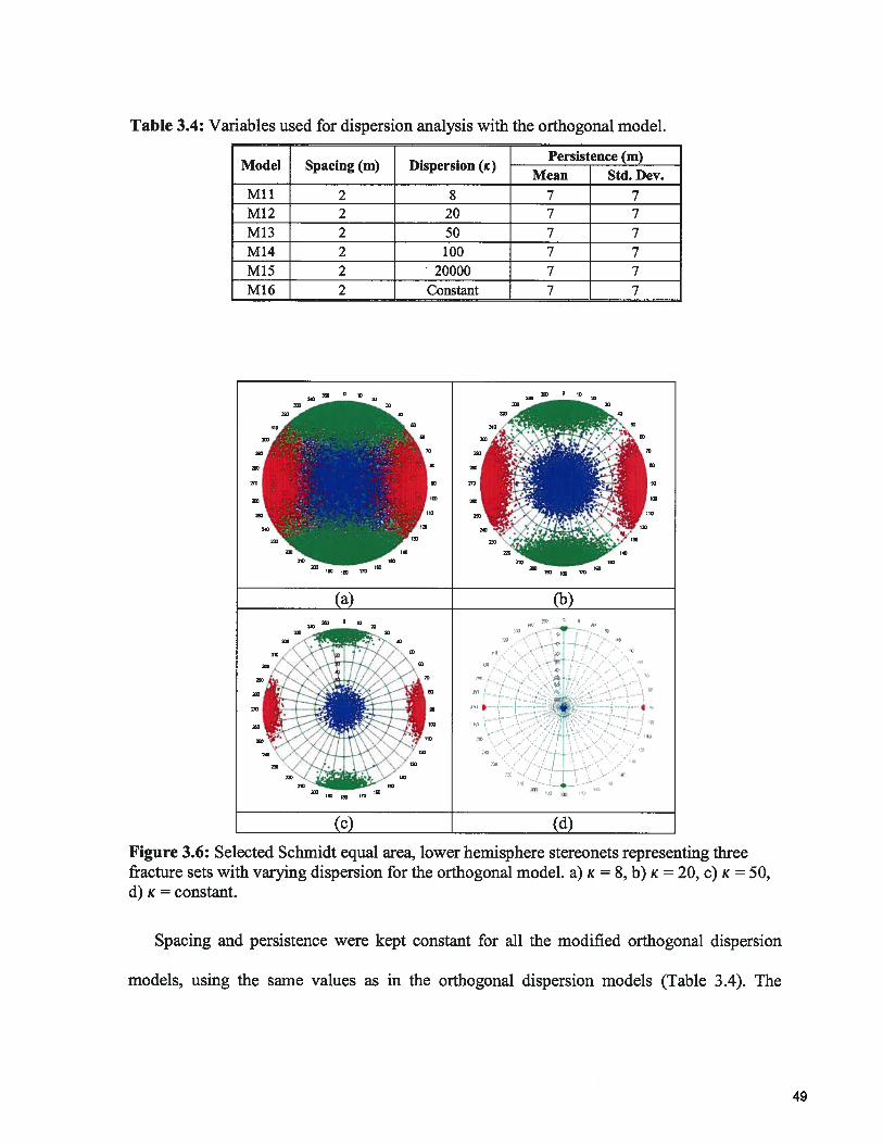
Table 3.4: Variables used for dispersion analysis with the orthogonal model.

Persistence (m)Model Spacing (m) Dispersion (K)

Mean Std. Dev.Mu 2 8 7 7M12 2 20 7 7M13 2 50 7 7M14 2 100 7 7M15 2 ‘20000 7 7M16 2 Constant 7 7

300 0 g y. 0

330— -—

10

30 , —.

43 301 - - 43

3W : --- —-

Zq1W :243

30

40

— —,

(c) (d)

Figure 3.6: Selected Schmidt equal area, lower hemisphere stereonets representing threefracture sets with varying dispersion for the orthogonal model. a) K = 8, b) K = 20, c) K = 50,d) K = constant.

Spacing and persistence were kept constant for all the modified orthogonal dispersion

models, using the same values as in the orthogonal dispersion models (Table 3.4). The

34010

10

(a) (1,)

49

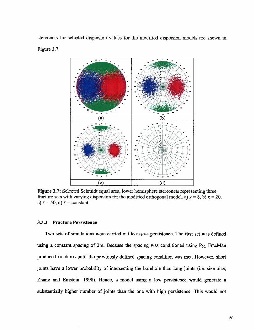
stereonets for selected dispersion values for the modified dispersion models are shown in

Figure 3.7.

3.3.3 Fracture Persistence

Two sets of simulations were canied out to assess persistence. The first set was defined

using a constant spacing of 2m. Because the spacing was conditioned using Pio, FracMan

produced fractures until the previously defined spacing condition was met. However, short

joints have a lower probability of intersecting the borehole than long joints (i.e. size bias;

Zhang and Einstein, 1998). Hence, a model using a low persistence would generate a

substantially higher number of joints than the one with high persistence. This would not

(a)

/

2/ S

(c) (d)

Figure 3.7: Selected Schmidt equal area, lower hemisphere stereonets representing threefracture sets with varying dispersion for the modified orthogonal model. a) K = 8, b) K = 20,c) K = 50, d) K = constant.

50

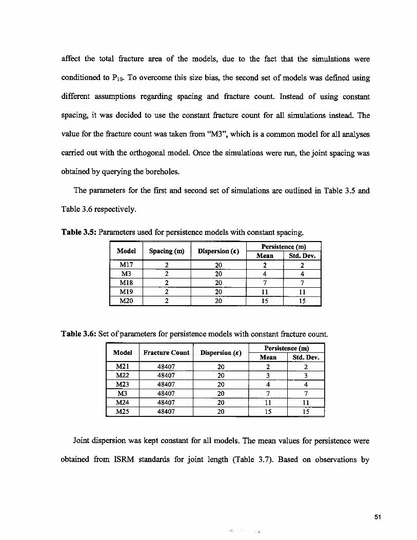
affect the total fracture area of the models, due to the fact that the simulations were

conditioned to P10. To overcome this size bias, the second set of models was defined using

different assumptions regarding spacing and fracture count. Instead of using constant

spacing, it was decided to use the constant fracture count for all simulations instead. The

value for the fracture count was taken from “M3”, which is a common model for all analyses

carried out with the orthogonal model. Once the simulations were run, the joint spacing was

obtained by querying the boreholes.

The parameters for the first and second set of simulations are outlined in Table 3.5 and

Table 3.6 respectively.

Table 3.5: Parameters used for persistence models with constant spacing.

Model Spacing (m) Dispersion (K)Persistence (m)

Mean Std. Dev.M17 2 20 2 2M3 2 20 4 4

M18 2 20 7 7M19 2 20 11 11M20 2 20 15 15

Table 3.6: Set of parameters for persistence models with constant fracture count.

Persistence (m)Model Fracture Count Dispersion (K)

Mean Std. Dev.M21 48407 20 2 2M22 48407 20 3 3M23 48407 20 4 4M3 48407 20 7 7

M24 48407 20 11 11M25 48407 20 15 15

Joint dispersion was kept constant for all models. The mean values for persistence were

obtained from ISRM standards for joint length (Table 3.7). Based on observations by

51

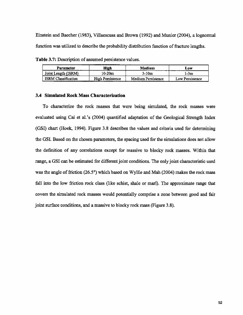
Einstein and Baecher (1983), Villaescusa and Brown (1992) and Munier (2004), a lognormal

function was utilized to describe the probability distribution function of fracture lengths.

Table 3.7: Description of assumed persistence values.

Parameter High Medium LowJoint Length (ISRM) 1O-20m 3-lOm 1-3mISRIvI Classification High Persistence Medium Persistence Low Persistence

3.4 Simulated Rock Mass Characterization

To characterize the rock masses that were being simulated, the rock masses were

evaluated using Cai et al.’s (2004) quantified adaptation of the Geological Strength Index

(GSI) chart (Hoek, 1994). Figure 3.8 describes the values and criteria used for determining

the GSI. Based on the chosen parameters, the spacing used for the simulations does not allow

the definition of any correlations except for massive to blocky rock masses. Within that

range, a GSI can be estimated for different joint conditions. The only joint characteristic used

was the angle of friction (26.5°) which based on Wyllie and Mah (2004) makes the rock mass

fall into the low friction rock class (like schist, shale or marl). The approximate range that

covers the simulated rock masses would potentially comprise a zone between good and fair

joint surface conditions, and a massive to blocky rock mass (Figure 3.8).

52

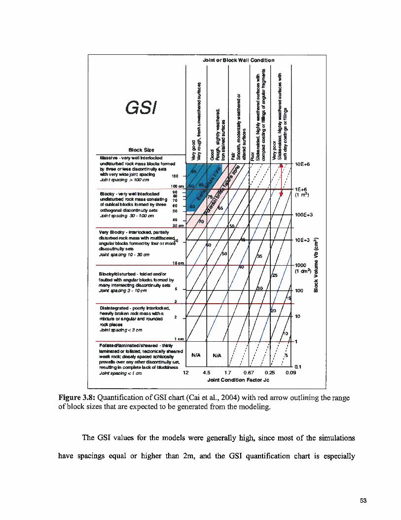
Joint or Block Wall Condition

GSI

Block Size

Mass.Ive very wel rler$ocked

ixsturbed rock rss l,iocks formedy tree or less s1emy salewI very wideoe1 5CWQ

Aen3aang> l(YJcm

Blocky e ry wel m1elocedtxsturbed rocic itleSS Qz

otQabb1(5 nTled bythree

orthogoisJ eorIrt4’ eelsntaong 30- fQQ,

Vely Blocky - r1erk,d(ed. parsaly

SL rDed rock mass witi miItitsce1ec0anguler biaclis tomled by ur or moresou1rviy saleJonr aang 10 - 30 i

Disintegrated - poorly rlerIaad.heady brc4en ro mass Th arrjre orargiAar and rorided

racir piecesJointaang3cm

E(3

.0

FatedIaminated/shearecl - Iraly

lamreded or baled, teclorcaIy beredweak rock; ciosey spaced xIs)ssyprais owr anyoesocnlruny eel,resARg r corpele lack of biaclcreas

Jc.,t spacwig I cn 12 4.5 1J 0.67 0.25

Joint Condition Factor Jc

Figure 3.8:ofblock sizes that are expected to be generated from the modeling.

Quantification of GSI chart (Cai et al., 2004) with red arrow outlining the range

The GSI values for the models were generally high, since most of the simulations

have spacings equal or higher than 2m, and the GSI quantification chart is especially

100 ‘r

90so106050

40

BlockyAdisturbed keded andiorta*Med anAarb4aca rmed bymany .leraec9 srrctrtMy saleJoint aang3- 10cm

0.09

53

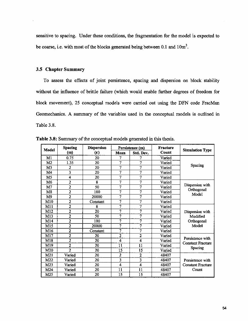
sensitive to spacing. Under these conditions, the fragmentation for the model is expected to

be coarse, i.e. with most of the blocks generated being between 0.1 and 10m3.

3.5 Chapter Summary

To assess the effects of joint persistence, spacing and dispersion on block stability

without the influence of brittle failure (which would enable further degrees of freedom for

block movement), 25 conceptual models were carried out using the DFN code FracMan

Geomechanics. A summary of the variables used in the conceptual models is outlined in

Table 3.8.

Table 3.8: Summary of the conceptual models generated in this thesis.

Spacing Dispersion Persistence (m) FractureModel Simulation Type

(m) (K) Mean Std. Dev. CountMl 0.75 20 7 7 VariedM2 1.35 20 7 7 VariedM3 2 20 7 7 Varied

Spacing

M4 3 20 7 7 VariedMS 4 20 7 7 VariedM6 2 8 7 7 VariedM7 2 50 7 7 Varied Dispersion with

M8 2 100 7 7 VariedOrthogonal

ModelM9 2 20000 7 7 VariedMl 0 2 Constant 7 7 VariedMu 2 8 7 7 VariedM12 2 20 7 7 Varied Dispersion withM13 2 50 7 7 Varied ModifiedM14 2 100 7 7 Varied OrthogonalMiS 2 20000 7 7 Varied ModelMl 6 2 Constant 7 7 VariedM17 2 20 2 2 Varied

Persistence withM18 2 20 4 4 VariedConstant Fracture

M19 2 20 11 11 VariedSpacing

M20 2 20 15 15 VariedM21 Varied 20 2 2 48407M22 Varied 20 3 3 48407 Persistence withM23 Varied 20 4 4 48407 Constant FractureM24 Varied 20 11 11 48407 CountM25 Varied 20 15 15 48407

54

The assembled model consisted of three parts: an outer box representing the rock mass,

an inner box representing the ore body and a slab under the inner box representing the

undercut. FracMan Geomechanics conducted a block stability analysis based on Goodman

and Shi’s (1985) block theory and calculated the factor of safety based on the Mohr-Coulomb

criterion for free falling blocks, blocks sliding on one and two faces, and stable blocks.

55

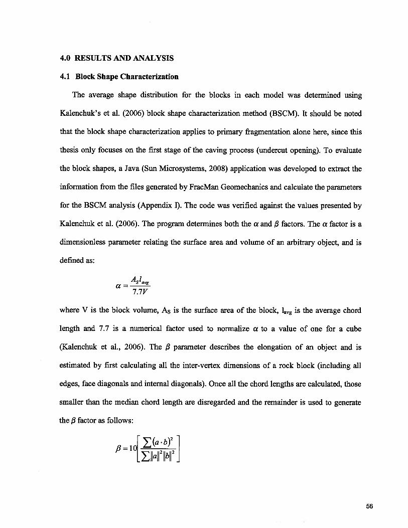
4.0 RESULTS AND ANALYSIS

4.1 Block Shape Characterization

The average shape distribution for the blocks in each model was determined using

Kalenchuk’s et al. (2006) block shape characterization method (BSCM). It should be noted

that the block shape characterization applies to primary fragmentation alone here, since this

thesis only focuses on the first stage of the caving process (undercut opening). To evaluate

the block shapes, a Java (Sun Microsystems, 2008) application was developed to extract the

information from the files generated by FracMan Geomechanics and calculate the parameters

for the BSCM analysis (Appendix I). The code was verified against the values presented by

Kalenchuk et al. (2006). The program determines both the a and 3 factors. The a factor is a

dimensionless parameter relating the surface area and volume of an arbitrary object, and is

defined as:

Aslavg

7.7V

where V is the block volume, A5 is the surface area of the block, lavg is the average chord

length and 7.7 is a numerical factor used to normalize a to a value of one for a cube

(Kalenchuk et al., 2006). The 3 parameter describes the elongation of an object and is

estimated by first calculating all the inter-vertex dimensions of a rock block (including all

edges, face diagonals and internal diagonals). Once all the chord lengths are calculated, those

smaller than the median chord length are disregarded and the remainder is used to generate

the /3 factor as follows:

(a .b)2/3=10

bN2

56

where a and b are the combination of chords equal or larger than the median chord length

(Kalenchuk et al., 2006). As described in section 2.2, blocks are classified according to their

shape based on three main groups:

• Cubic (C);

• Elongated (E);

• Platy (P);

and three transitional shape groups:

• Cubic-Elongated (CE);

• Elongated-Platy (EP); and

• Platy-Cubic (PC).

The average values of the simulations were utilized for the evaluation of the block

shapes. The analysis was also carried out only on single blocks and only blocks larger than

0.001m3were examined.

The shape distribution for the FracMan spacing simulations is described in Figure 4.1. In

the smallest spacing (model Ml), most of the blocks are cubic, cubic-elongated and

elongated, with less platy-cubic and elongated-platy. However, as spacing increases the

blocks distribution changes. The number of cubic blocks shows a progressive decrease and a

clustering of the points starts to develop in the elongated block region of the diagram. This is

especially noticeable in models M2 and M3 and is confirmed by observing the shape

distribution plots. As the spacing further increases, most of the blocks become elongated.

Still, for some of the spacing simulations it can be observed that all six shape types are

generated. It would be expected that the generated rock masses would be primarily composed

of equidimensional blocks, since the properties of all three joint sets are the same. This does

57

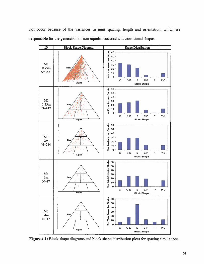
not occur because of the variances in joint spacing, length and orientation, which are

responsible for the generation of non-equidimensional and transitional shapes.

ID Block Shape Diagram Shape Distribution

MlBe/1..\

10

,‘ \ \ C C-E E E-P p p-cA1ba Block Shape

60 —

0ccEEppp.c

Block Shape

N=244

/: \ \ c c-E E E-P p p-cAlpha

Block Shape

60

;4\ OC(>EEEPppC

A1Ph Block Shape

f 60

. 5O

B,/4\CCEEE-PPP-C

AlphaBlock Shape

Figure 4.1: Block shape diagrams and block shape distribution plots for spacing simulations.

58

For the original dispersion models (Figure 4.2), the low K values (model M6) result in a

clustering of the points in the elongated and cubic-elongated areas of the block shape

diagram. As expected for this orthogonal model with equally spaced joints, the blocks

become more equidimensional as the K value increases. When K is constant, most of the

blocks are either cubic or cubic-elongated. However, there are still blocks in the elongated

and platy-cubic areas, due to the variations in discontinuity spacing and persistence.

The modified dispersion models show similar trends as the original dispersion models

(Figure 4.3). For low K values (K equal to 8 and 20) there is a slightly higher occurrence of

cubic block than cubic-elongated and elongated blocks. This differs from the original

dispersion models in Figure 4.2 which show a tendency of forming more cubic-elongated

blocks. The difference between the original dispersion and modified dispersion models is

credited to the orientation difference of two of the joint sets. For intermediate K values (K

equal to 50 and 100) there is a small increase in the amount of elongated blocks. This

changes as K is further increased. As expected (and similar to the original dispersion models),

when dispersion is constant most blocks are equidimensional (cubic). Nevertheless, there are

a large percentage of elongated cubic and elongated blocks, as well as a smaller quantity of

platy-cubic blocks. The presence of other block shapes is again attributed to the variations in

discontinuity spacing and persistence in the models.

59

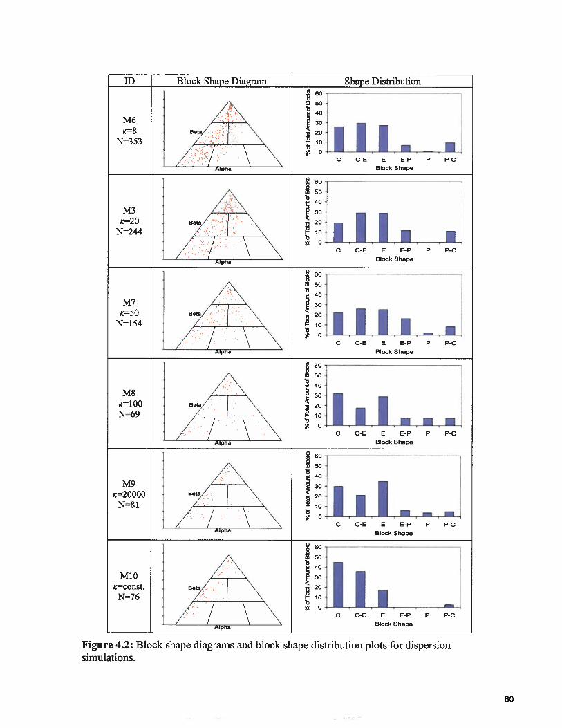
Figure 4.2: Block shape diagrams and block shape distribution plots for dispersionsimulations.

60

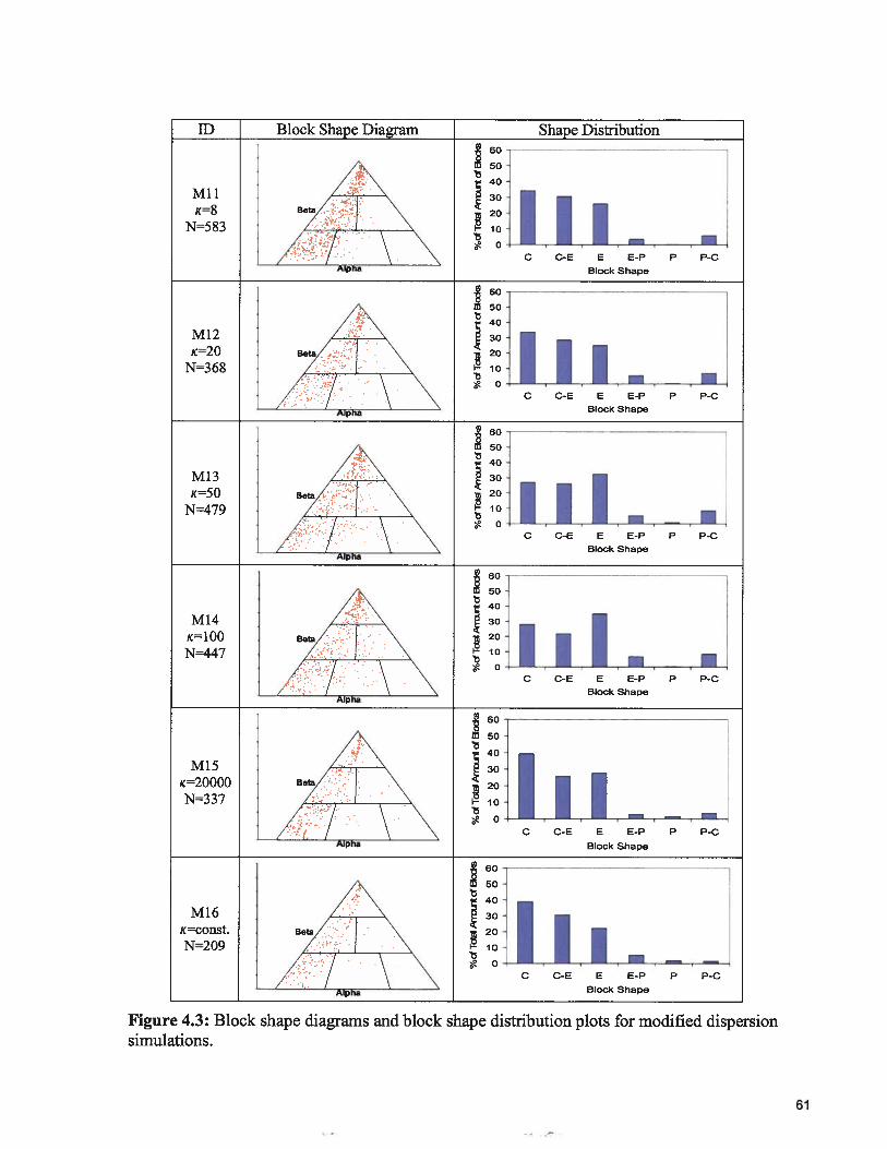
ID Block Shape Diagram Shape Distribution

N=583 LJI\\Alpha Block Shape

N=368

• Alpha Block Shape

60

50\

1(50

0CEEEPPPC

, Block ShapeAlpha

60

\ 50

0CCEEEPPP.C

, Block ShapeAlpha

/\\

K20000

0

CEEPPPCAlpha Block Shape

. 60

\ 50

KCOflStN I

CCEEEPPPC

Alpha Block Shape

Figure 4.3: Block shape diagrams and block shape distribution plots for modified dispersionsimulations.

61

In the persistence models with constant spacing, most of the rock masses generated are

dominated by elongated blocks (Figure 4.4). This is visible in the BSCM diagrams and the

shape distribution plots. As with the other simulations (spacing arid dispersion), different

block shapes were produced, most of them being cubic and cubic-elongated. As the mean

persistence is increased, blocks become more elongated and then cubic for the largest

persistence value. This occurs because longer fractures have more probability of intersecting

each other at regular intervals, therefore increasing the potential for generating more

equidimensional shapes. Some platy-cubic, platy and platy elongated blocks were also

produced, but most of the block shapes were again concentrated on the left side of the BSCM

diagram.

Persistence models with constant fracture count produce similar block shape distribution

patterns to the persistence models with constant spacing (Figure 4.5). In these simulations

however, the blocks formed by short joint lengths (3 and 4m) are concentrated mostly in the

elongated categories with no cubic and platy blocks being generated. As persistence is

increased, more cubic blocks and less elongated blocks are produced.

Almost all models have most of the block shapes concentrated on the left side of the

block shape diagram, i.e. cubic, cubic-elongated and elongated shapes. This can be attributed

to the assumptions utilized for the modeling. The properties of all three joint sets were the

same and only one variable was changed at a time. Since all the properties were the same, it

is expected that the blocks generated will be approximately equidimensional. The generation

of other shapes is a consequence of the range of values used for the variables (spacing,

dispersion and persistence). Kalenchuk et al. (2006) emphasized that in order to generate

different ranges of shapes in a three joint set model, the values of one or two joint sets need

62

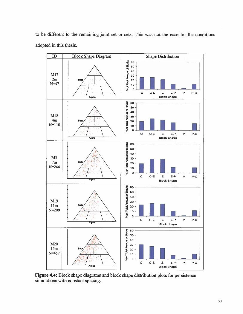
to be different to the remaining joint set or sets. This was not the case for the conditions

adopted in this thesis.

ID Block Shape Diagram Shape Distribution

M17 /\ J30

/ / \ \ c C-E E E-P P p-c

Alpha Block Shape

• 60

/ 50

/•\M18 3O

N=H8 4 \F

!Alpha Block Shape

60

M3 /•\N=244

/H\\\

/ c c-E E E-P p p-cAlpha Block Shape. 60

M19Urn

:1’ I11_w____.,,‘

c c-E E E-P P P-cAlpha

Block Shape. 60

\ 50‘\

N=457 I IiI_rLr__•1 c c-E E E-P p p-c

Alpha Block Shape

Figure 4.4: Block shape diagrams and block shape distribution plots for persistencesimulations with constant spacing.

63

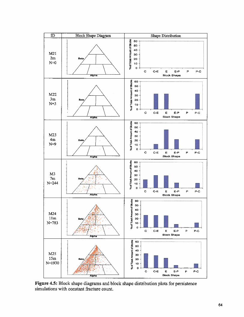
ID Block Shape Diagram Shape Distribution

• 60

M21 A

2m Beta/ 20

N=O /

/ / \ \

0C-E E E-P P P-c

Alpha Block Shape

M22

Be/\

Alpha Block Shape

60

i 7 1CCEEE-P PP-C

Alpha Block Shape

60

M3//\

N=244

CCEEE-PPP-CIha Block Shape

. 60

50

/\ 40

M24 30

N=783 \ CCEEEPPPC

‘Alpha Block Shape

60

/ 50

/‘•“.40

N=1930Beta/’”\ I

CC-EEE-P PP-C

Alpha Block Shape

Figure 4.5: Block shape diagrams and block shape distribution plots for persistencesimulations with constant fracture count.

64

4.2 Block Failure Mode

FracMan can provide information about the mode of failure of each block as part of its

output. The failure types are divided into four categories: free falling, sliding on one plane,

sliding on two planes and stable. The factor of safety of blocks sliding on one or two faces is

estimated using the Mohr-Coulomb failure criterion (chapter 3.1). FracMan classifies the

block failures in four types: the free falling, sliding on one plane blocks, sliding on two

planes and stable blocks. Free falling blocks have a factor of safety less than one. Blocks

sliding on one or two planes can have factors of safety greater or less than one. Stable blocks

have a factor of safety greater than one. Under this defmition, blocks free falling and sliding

(on one or two planes) with a factor of safety less than one are considered key blocks

(unstable block volume). The rest of the blocks are potential key blocks or tapered blocks

(stable block volume). The results for the analysis of each model are described as a

percentage of the total block volume generated and as a percentage of the total number of

blocks. Only blocks larger than 0.00 1 m3 were examined.

Table 4.1 and Figure 4.6a and 4.6b show the failure type occurrence for the spacing

simulations. Most of the block volume generated is stable with very little volume

corresponding to blocks sliding on two planes Figure 4.6a. The unstable block volume is

mostly composed of blocks sliding on one face with the free falling block volume

representing approximately 20% of the total unstable block volume. By comparing the

amount of blocks corresponding to each failure type (Figure 4.6b) to the volumes in Figure

4.6a, it can be inferred that the stable blocks have the largest volumes and the blocks sliding

on two faces have the smallest. It can also be observed that most the blocks for model M5 are

sliding on one face, however the largest volume is still represented by the stable blocks. The

65

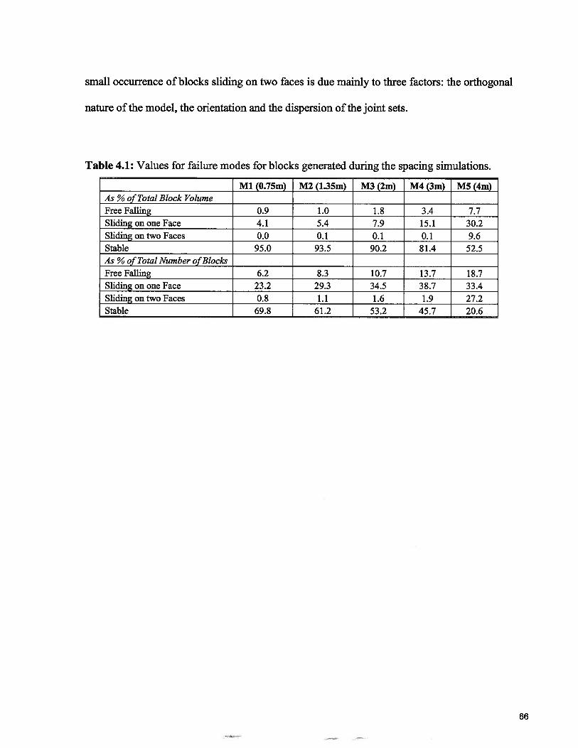
small occurrence of blocks sliding on two faces is due mainly to three factors: the orthogonal

nature of the model, the orientation and the dispersion of the joint sets.

Table 4.1: Values for failure modes for blocks generated during the spacing simulations.

Ml (O.75m) M2 (l.35m) M3 (2m) M4 (3m) M5 (4m)As % of Total Block VolumeFree Falling 0.9 1.0 1.8 3.4 7.7Sliding on one Face 4.1 5.4 7.9 15.1 30.2Sliding on two Faces 0.0 0.1 0.1 0.1 9.6Stable 95.0 93.5 90.2 81.4 52.5As % of Total Number ofBlocksFree Falling 6.2 8.3 10.7 13.7 18.7SlidingononeFace 23.2 29.3 34.5 38.7 33.4Sliding on two Faces 0.8 1.1 1.6 1.9 27.2Stable 69.8 61.2 53.2 45.7 20.6

66

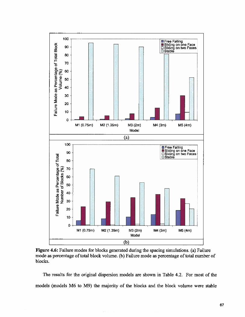
100

C.)0

- 80

70

60

50cD2

Ml (0.75m) M2 (1 .35m) M3 (2m) M4 (3m) M5 (4m)

Model

(a)

100• Free Falling•Sliding on one Face

— 90 c:lSlidingontwoFacesStable

804-0

__

70

6000

40ci) .D

0z 30

Ml (0.75m) M2 (1 .35m) M3 (2m) M5 (4m)Model

(b)

Figure 4.6: Failure modes for blocks generated during the spacing simulations. (a) Failuremode as percentage of total block volume. (b) Failure mode as percentage of total number ofblocks.

The results for the original dispersion models are shown in Table 4.2. For most of the

models (models M6 to M9) the majority of the blocks and the block volume were stable

• Free FallingI •Sliding on one FaceI 0 Sliding on two FacesLLStable

-.-IjJ

M4 (3m)

67

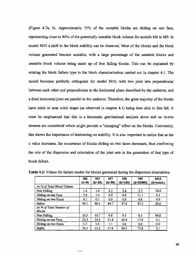
(Figure 4.7a, b). Approximately 75% of the unstable blocks are sliding on one face,

representing close to 80% of the potentially unstable block volume for models M6 to M9. In

model M10 a shift in the block stability can be observed. Most of the blocks and the block

volume generated become unstable, with a large percentage of the unstable blocks and

unstable block volume being made up of free falling blocks. This can be explained by

relating the block failure type to the block characterization carried out in chapter 4.1. The

model becomes perfectly orthogonal for model M10, with two joint sets perpendicular

between each other and perpendicular to the horizontal plane described by the undercut, and

a third horizontal joint set parallel to the undercut. Therefore, the great majority of the blocks

have cubic or near cubic shape (as observed in chapter 4.1) being then able to free fall. It

must be emphasized that this is a kinematic gravitational analysis alone and no in-situ

stresses are considered which might provide a “clamping” effect on the blocks. Conversely,

this shows the importance of destressing on stability. It is also important to notice that as the

K value increases, the occurrence of blocks sliding on two faces decreases, thus confirming

the role of the dispersion and orientation of the joint sets in the generation of that type of

block failure.

Table 4.2: Values for failure modes for blocks generated during the dispersion simulations.

M6 M3 M7 M8 M9 M1O(k=8) (k=20) (k=50) (k=100) (k=20000) (k=const.)

As % of Total Block VolumeFree Falling 1.6 1.8 2.3 2.6 3.7 70.9Sliding on one Face - 7.6 7.9 8.0 9.8 11.1 0.1Sliding on two Faces 0.1 0.1 0.0 0.0 0.0 0.0Stable 90.7 90.2 89.7 87.6 85.2 29.0As % of Total Number ofBlocksFree Falling 10.5 10.7 9.8 9.5 6.3 94.8Sliding on one Face 33.5 34.5 31.4 29.4 17.9 0.1Sliding on two Faces 1.7 1.6 1.1 0.6 0.0 0.0Stable 54.3 53.2 57.8 60.5 75.8 5.1

68

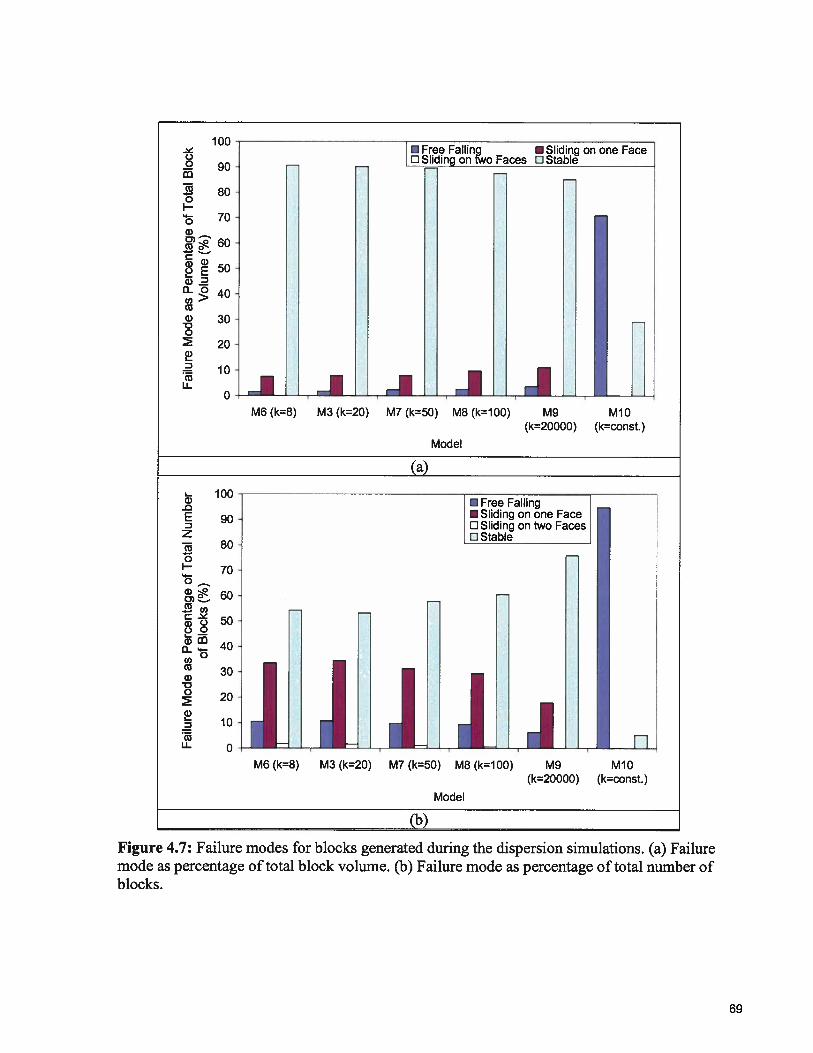
100

9o

80

70Ci)

60

5052

40

300

20

10Cu

U-0

M6 (k=8) M3 (k=20) M7 (k=50) M8 (k=100) M9 M10(k=20000) (k=const.)

Model

(a)

L 100•Free Falling

E 90 • Sliding on one FaceD 0 Sliding on two FacesZ 0 Stable

800

700__..

60

fi: :J rJL] J 1 HM6 (k=8) M3 (k=20) M7 (k=50) M8 (k=100) M9 M10

(k=20000) (k=const.)

Model

(b)

Figure 4.7: Failure modes for blocks generated during the dispersion simulations. (a) Failuremode as percentage of total block volume. (b) Failure mode as percentage of total number ofblocks.

• Free Falling • Sliding on one Face0 Shding on two Faces 0 Stable

_i_i_iJJ

69

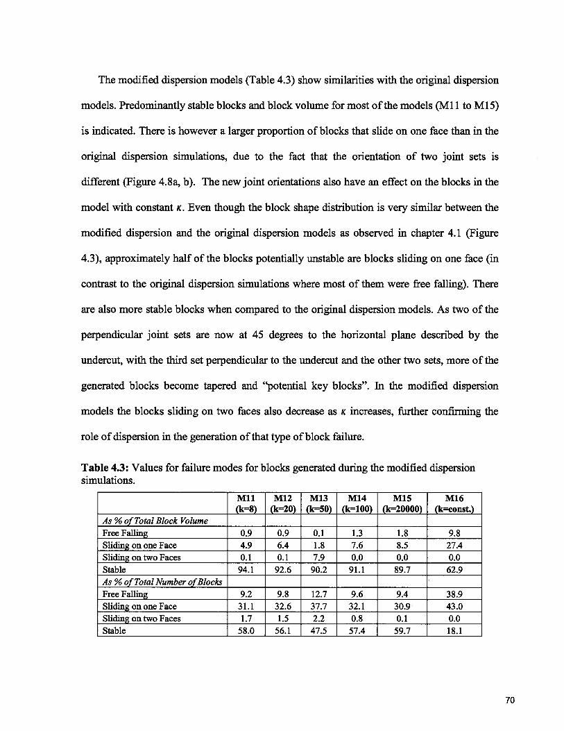
The modified dispersion models (Table 4.3) show similarities with the original dispersion

models. Predominantly stable blocks and block volume for most of the models (Ml 1 to M15)

is indicated. There is however a larger proportion of blocks that slide on one face than in the

original dispersion simulations, due to the fact that the orientation of two joint sets is

different (Figure 4.8a, b). The new joint orientations also have an effect on the blocks in the

model with constant K. Even though the block shape distribution is very similar between the

modified dispersion and the original dispersion models as observed in chapter 4.1 (Figure

4.3), approximately half of the blocks potentially unstable are blocks sliding on one face (in

contrast to the original dispersion simulations where most of them were free falling). There

are also more stable blocks when compared to the original dispersion models. As two of the

perpendicular joint sets are now at 45 degrees to the horizontal plane described by the

undercut, with the third set perpendicular to the undercut and the other two sets, more of the

generated blocks become tapered and “potential key blocks”. In the modified dispersion

models the blocks sliding on two faces also decrease as K increases, further confirming the

role of dispersion in the generation of that type of block failure.

Table 4.3: Values for failure modes for blocks generated during the modified dispersionsimulations.

Mu M12 M13 M14 M15 M16(k=8) (k=20) (k=50) (k=100) (k=20000) (k=const.)

As % of Total Block VolumeFree Falling 0.9 0.9 0.1 1.3 1.8 9.8Sliding on one Face 4.9 6.4 1.8 7.6 8.5 27.4Sliding on two Faces 0.1 0.1 7.9 0.0 0.0 0.0Stable 94.1 92.6 90.2 91.1 89.7 62.9As % of Total Number ofBlocksFree Falling 9.2 9.8 12.7 9.6 9.4 38.9Sliding on one Face 31.1 32.6 37.7 32.1 30.9 43.0Sliding on two Faces 1.7 1.5 2.2 0.8 0.1 0.0Stable 58.0 56.1 47.5 57.4 59.7 18.1

70

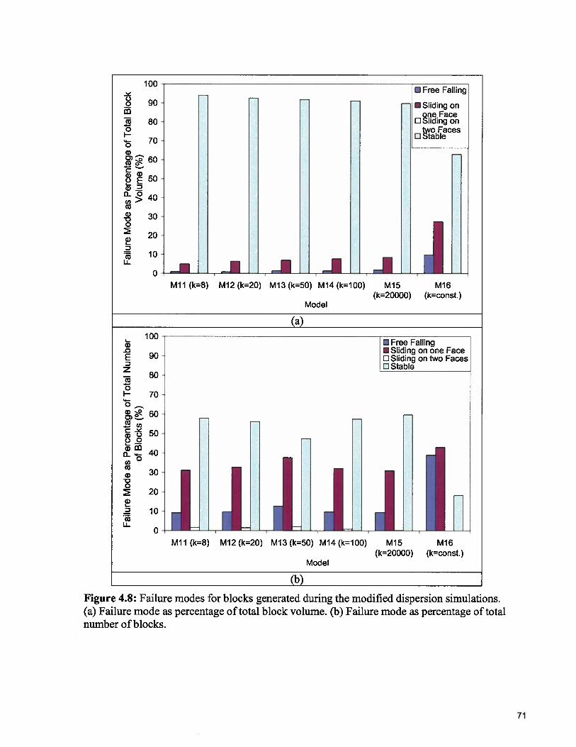
100• Free Falling I

1001

C)

EDz

0I0

60

C) 50—_ 40

30

90

80

70

20

10

0

(a)

Mu (k=8) M12(k=20) M13(k=50) M14(k=100)

(b)

Model

M15 M16(k=20000) (k=const.)

Figure 4.8: Failure modes for blocks generated during the modified dispersion simulations.(a) Failure mode as percentage of total block volume. (b) Failure mode as percentage of totalnumber of blocks.

00

I

90

80

70

60

0)50

D0> 40

30

20

10

0

• Sliding onoeFace

C Sliding ontwo Faces

C Stable

-. _I_I _I IIMu (k=8) M12(k=20) M13(k=50) M14(k=100) M15 M16

(k20000) (k=const.)Model

• Free Falling• Sliding on one FaceC Sliding on two FacesC Stable

II I H

71

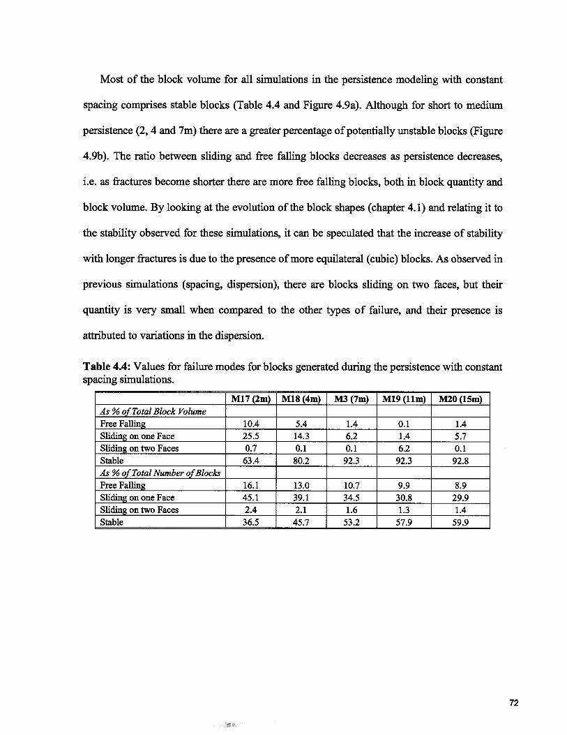
Most of the block volume for all simulations in the persistence modeling with constant

spacing comprises stable blocks (Table 4.4 and Figure 4.9a). Although for short to medium

persistence (2, 4 and 7m) there are a greater percentage of potentially unstable blocks (Figure

4.9b). The ratio between sliding and free falling blocks decreases as persistence decreases,

i.e. as fractures become shorter there are more free falling blocks, both in block quantity and

block volume. By looking at the evolution of the block shapes (chapter 4.1) and relating it to

the stability observed for these simulations, it can be speculated that the increase of stability

with longer fractures is due to the presence of more equilateral (cubic) blocks. As observed in

previous simulations (spacing, dispersion), there are blocks sliding on two faces, but their

quantity is very small when compared to the other types of failure, and their presence is

attributed to variations in the dispersion.

Table 4.4: Values for failure modes for blocks generated during the persistence with constantspacing simulations.

M17(2m) M18(4m) M3(7m) M19(llm) M20(15m)As % of Total Block VolumeFree Falling 10.4 5.4 1.4 0.1 1.4Sliding on one Face 25.5 14.3 6.2 1.4 5.7Sliding on two Faces 0.7 0.1 0.1 6.2 0.1Stable 63.4 80.2 92.3 92.3 92.8As % ofTotal Number ofBlocksFree Falling 16.1 13.0 10.7 9.9 8.9Sliding on one Face 45.1 39.1 34.5 30.8 29.9Sliding on two Faces 2.4 2.1 1.6 1.3 1.4Stable 36.5 45.7 53.2 57.9 59.9

72

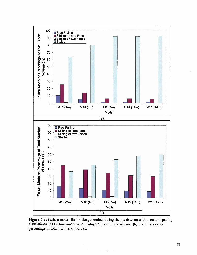
100-

C)0

- 80

70

60

50

00CC> 40C)C)

1::

• Free Falling•Sliding on one FaceD Silding on two FacesEl Stable

.1M17 (2m) M18 (4m) M3 (7m) M19 (urn) M20 (15m)

Model

(a)

C)-

2zC)

IU0

C)C -

CC.)0.2C)

COC)C)

0

C)U-

100

90

80

70

60

50

40

30

20

10

0

• Free Falling• Sliding on one FaceEl Sliding on two FacesEl Stable

ElL1

M17 (2m) M18 (4m) M3 (7rn)

Model

M19(llm)

(b)

M20 (15m)

Figure 4.9: Failure modes for blocks generated during the persistence with constant spacingsimulations. (a) Failure mode as percentage of total block volume. (b) Failure mode aspercentage of total number ofblocks.

73

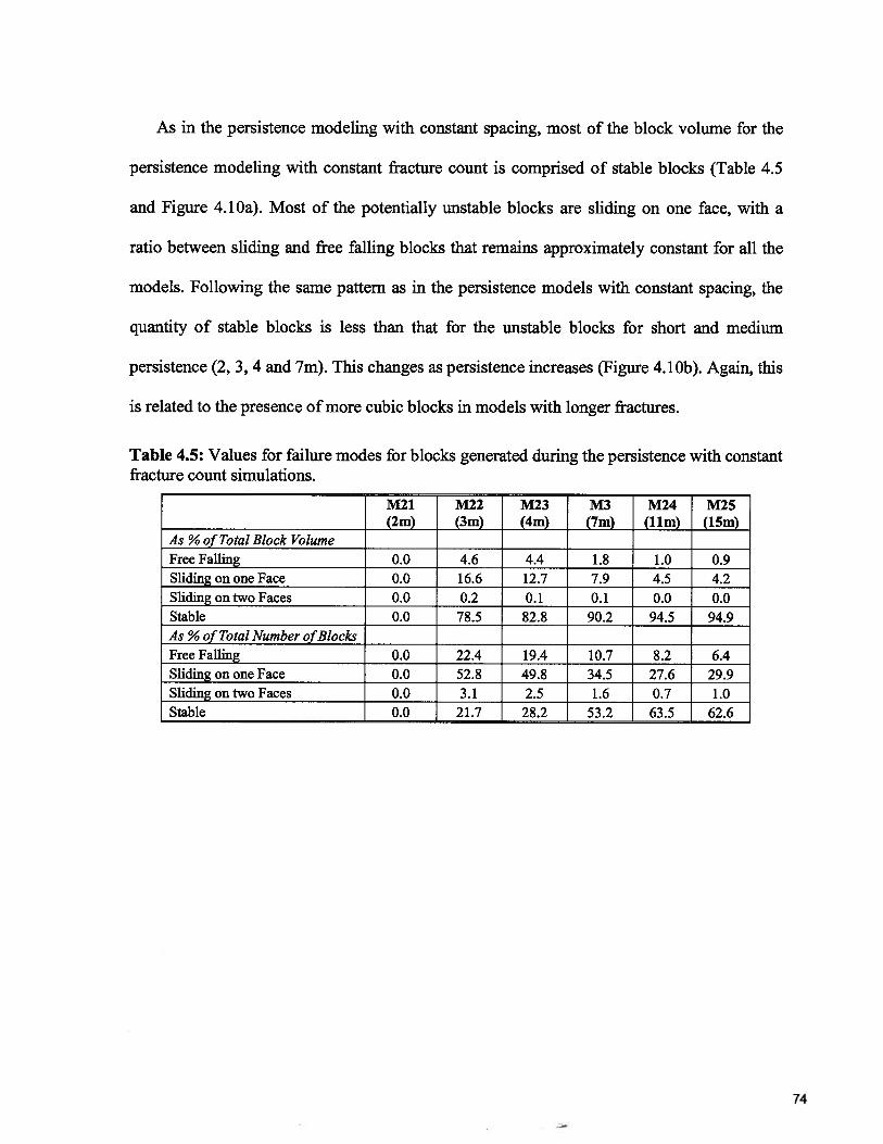
As in the persistence modeling with constant spacing, most of the block volume for the

persistence modeling with constant fracture count is comprised of stable blocks (Table 4.5

and Figure 4.lOa). Most of the potentially unstable blocks are sliding on one face, with a

ratio between sliding and free falling blocks that remains approximately constant for all the

models. Following the same pattern as in the persistence models with constant spacing, the

quantity of stable blocks is less than that for the unstable blocks for short and medium

persistence (2, 3, 4 and 7m). This changes as persistence increases (Figure 4.1 Ob). Again, this

is related to the presence of more cubic blocks in models with longer fractures.

Table 4.5: Values for failure modes for blocks generated during the persistence with constantfracture count simulations.

M21 M22 M23 M3 M24 M25(2m) (3m) (4m) (7m) (urn) (15m)

As % of Total Block VolumeFree Falling 0.0 4.6 4.4 1.8 1.0 0.9Sliding on one Face 0.0 16.6 12.7 7.9 4.5 4.2Sliding on two Faces 0.0 0.2 0.1 0.1 0.0 0.0Stable 0.0 78.5 82.8 90.2 94.5 94.9As % of Total Number ofBlocksFree Falling 0.0 22.4 19.4 10.7 8.2 6.4Sliding on one Face 0.0 52.8 49.8 34.5 27.6 29.9Sliding on two Faces 0.0 3.1 2.5 1.6 0.7 1.0Stable 0.0 21.7 28.2 53.2 63.5 62.6

74

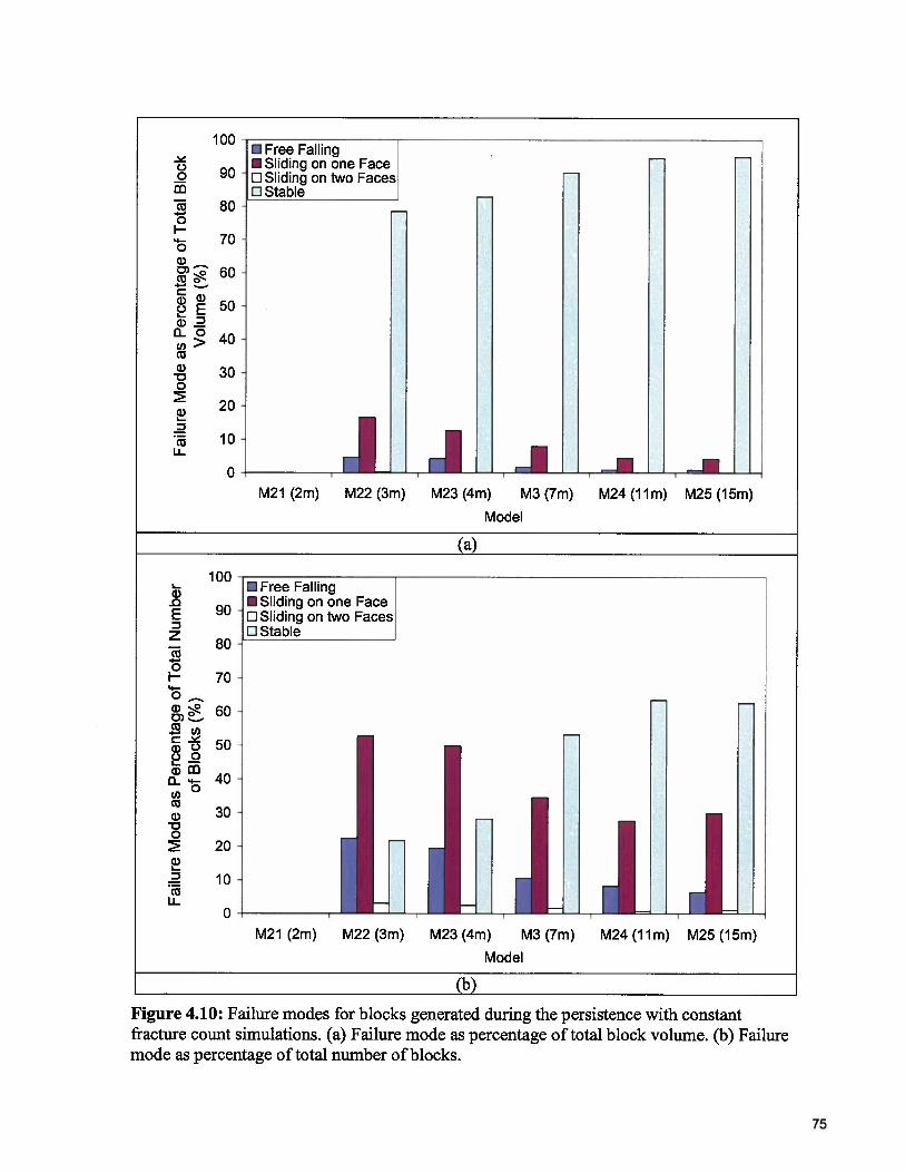
100

90

80

70

60

30

20

10

0

Model

C)0

Cu0I

0V

50

D0 40Cu

0

CuLI

• Free Falling• Sliding on one Face[:JSliding on two FacesStable

M21 (2m) M22 (3m) M23 (4m) M3 (7m) M24 (11 m) M25 (1 5m)

(a)

100• Free Falling• Sliding on one Face

Sliding on two FacesE Stable

ci)

EDzCu0I0

I

0Cuci)

0

D

CuLL

80

70

60

50

40

30

20

10 jJIM21 (2m) M22 (3m) M23 (4m) M3 (7m) M24 (lim) M25 (15m)

Model

(b)

Figure 4.10: Failure modes for blocks generated during the persistence with constantfracture count simulations. (a) Failure mode as percentage of total block volume. (b) Failuremode as percentage of total number of blocks.

75

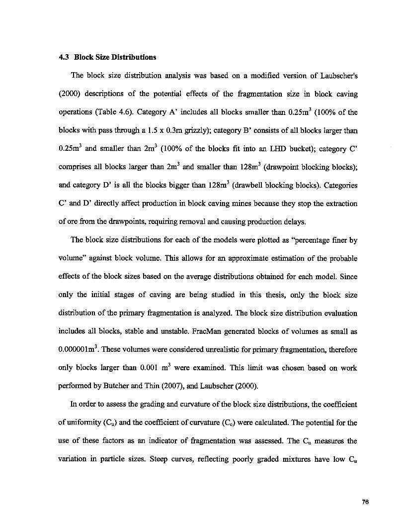
4.3 Block Size Distributions

The block size distribution analysis was based on a modified version of Laubscher’s

(2000) descriptions of the potential effects of the fragmentation size in block caving

operations (Table 4.6). Category A’ includes all blocks smaller than 0.25m3 (100% of the

blocks with pass through a 1.5 x 0.3m grizzly); category B’ consists of all blocks larger than

0.25m3 and smaller than 2m3 (100% of the blocks fit into an LHD bucket); category C’

comprises all blocks larger than 2m3 and smaller than 128m3 (drawpoint blocking blocks);

and category D’ is all the blocks bigger than 128m3 (drawbell blocking blocks). Categories

C’ and D’ directly affect production in block caving mines because they stop the extraction

of ore from the drawpoints, requiring removal and causing production delays.

The block size distributions for each of the models were plotted as “percentage finer by

volume” against block volume. This allows for an approximate estimation of the probable

effects of the block sizes based on the average distributions obtained for each model. Since

only the initial stages of caving are being studied in this thesis, only the block size

distribution of the primary fragmentation is analyzed. The block size distribution evaluation

includes all blocks, stable and unstable. FracMan generated blocks of volumes as small as

0.000001m3.These volumes were considered unrealistic for primary fragmentation, therefore

only blocks larger than 0.001 m3 were examined. This limit was chosen based on work

performed by Butcher and Thin (2007), and Laubscher (2000).

In order to assess the grading and curvature of the block size distributions, the coefficient

of uniformity (Ca) and the coefficient of curvature (Ce) were calculated. The potential for the

use of these factors as an indicator of fragmentation was assessed. The C measures the

variation in particle sizes. Steep curves, reflecting poorly graded mixtures have low C,

76

values, while flat curves reflecting well graded mixtures (or well sorted, in geological terms)

have high values (Coduto, 1999). The C value is based on the following formula:

D0U

I0

where D60 corresponds to the 60 percent passing (i.e. 60 percent of the blocks finer than D60)

and D10 is the 10 percent passing. The Cc describes the shape of the gradation curve. For

instance, materials with smooth curves have Cc values between 1 and 3, while most gap

graded materials have values outside this range (Coduto, 1999). The Cc is defined as follows:

=(]3)2

C D10D60

where D30 is the 30 percent passing, D10 is the 10 percent passing and D60 is the 60 percent

passing.

77

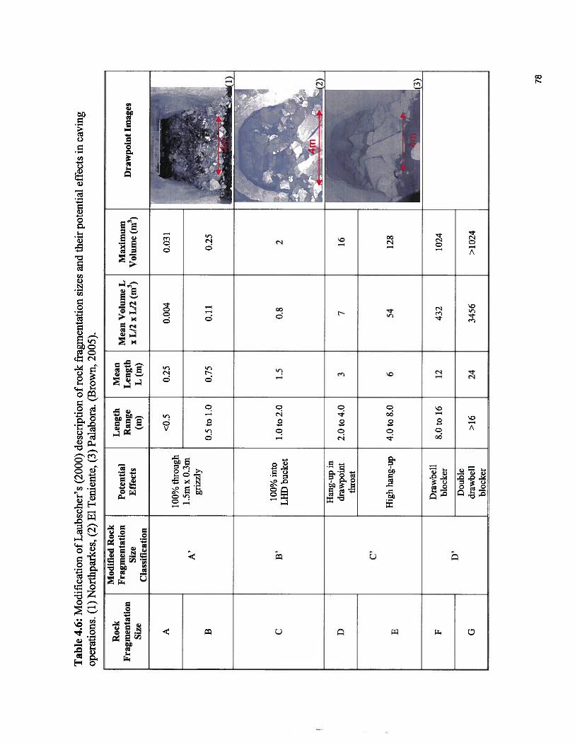
Tab

le4.

6:M

odif

icat

ion

ofL

aubs

cher

’s(2

000)

desc

ript

ion

ofro

ckfr

agm

enta

tion

size

san

dth

eir

pote

ntia

lef

fect

sin

cavi

ngop

erat

ions

.(1

)N

orth

park

es,

(2)

El

Ten

ient

e,(3

)Pa

labo

ra.

(Bro

wn,

2005

).

Mod

ifie

dR

ock

Roc

k.

.L

engt

hM

ean

.F

ragm

enta

tion

Pot

enti

alM

ean

Vol

ume

LM

axim

umF

ragm

enta

tion

.R

ange

Len

gth

33

Dra

wpo

int

Imag

es.

Size

Eff

ects

xL1

2x

L12

(m)

Vol

ume

(m)

Size

..

(m)

Lm

)C

lass

ific

atio

ni—

A<0

.50.

250.

004

0.03

110

0%th

roug

h

A’

1S

rnxO

3m

BO

5to

lO07

501

102

5

i

CB

’10

0%in

to1.

Oto

2.0

1.5

0.8

2L

HD

buck

et

(2)

Han

g-up

inD

draw

pom

t2.

Oto

4.0

37

16th

roat

C,

EH

ighh

ang-

up4.

0to

8.0

654

128

FD

raw

bell

8.0

to16

1243

210

24bl

ocke

rD

’D

oubl

eG

draw

bell

>16

2434

56>

1024

bloc

ker

() 78

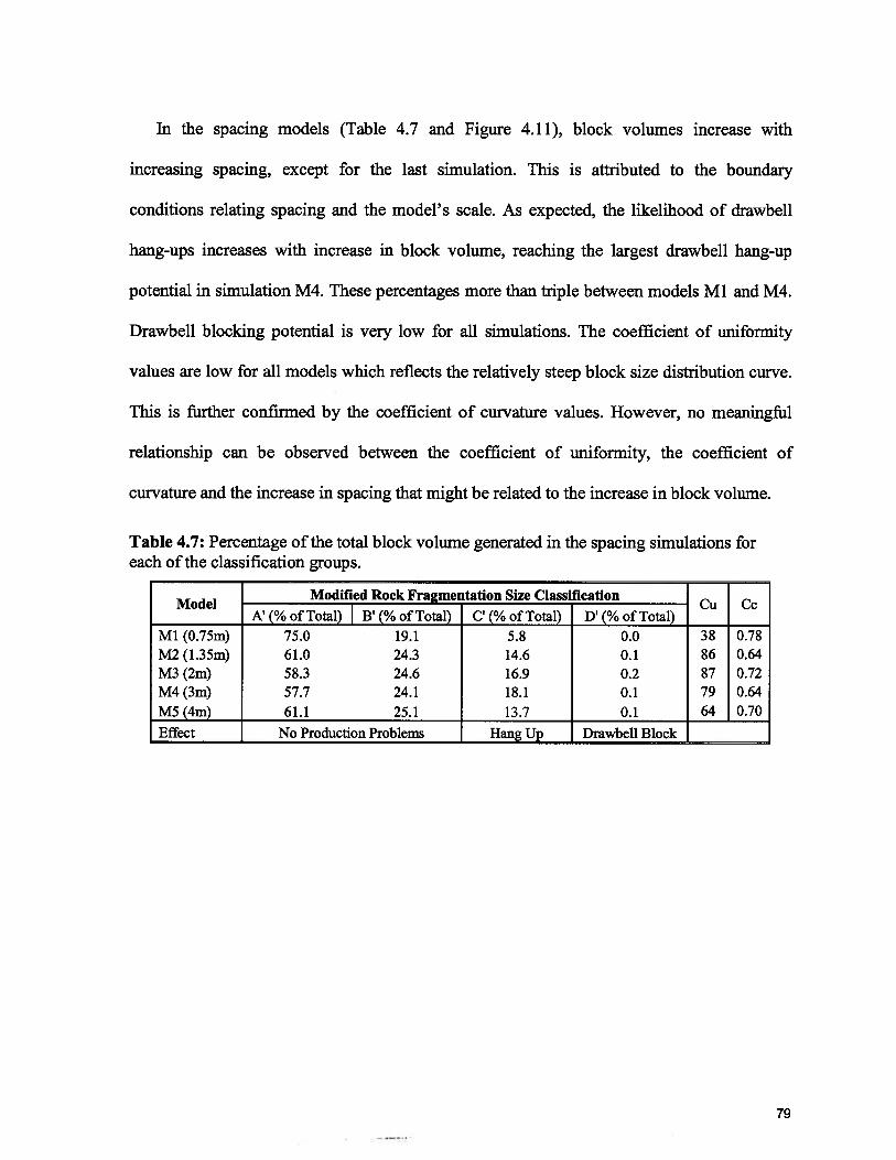
In the spacing models (Table 4.7 and Figure 4.11), block volumes increase with

increasing spacing, except for the last simulation. This is attributed to the boundary

conditions relating spacing and the model’s scale. As expected, the likelihood of drawbell

hang-ups increases with increase in block volume, reaching the largest drawbell hang-up

potential in simulation M4. These percentages more than triple between models Ml and M4.

Drawbell blocking potential is very low for all simulations. The coefficient of uniformity

values are low for all models which reflects the relatively steep block size distribution curve.

This is further confirmed by the coefficient of curvature values. However, no meaningful

relationship can be observed between the coefficient of uniformity, the coefficient of

curvature and the increase in spacing that might be related to the increase in block volume.

Table 4.7: Percentage of the total block volume generated in the spacing simulations foreach of the classification groups.

Modified Rock Fragmentation Size ClassificationModel Cu Cc

A’ (% of Total) B’ (% of Total) C’ (% of Total) D’ (% of Total) —

Ml (0.75m) 75.0 19.1 5.8 0.0 38 0.78M2 (1.35m) 61.0 24.3 14.6 0.1 86 0.64M3 (2m) 58.3 24.6 16.9 0.2 87 0.72M4 (3m) 57.7 24.1 18.1 0.1 79 0.64

MS (4m) 61.1 25.1 13.7 0.1 64 0.70

Effect No Production Problems Hang Up Drawbell Block

79

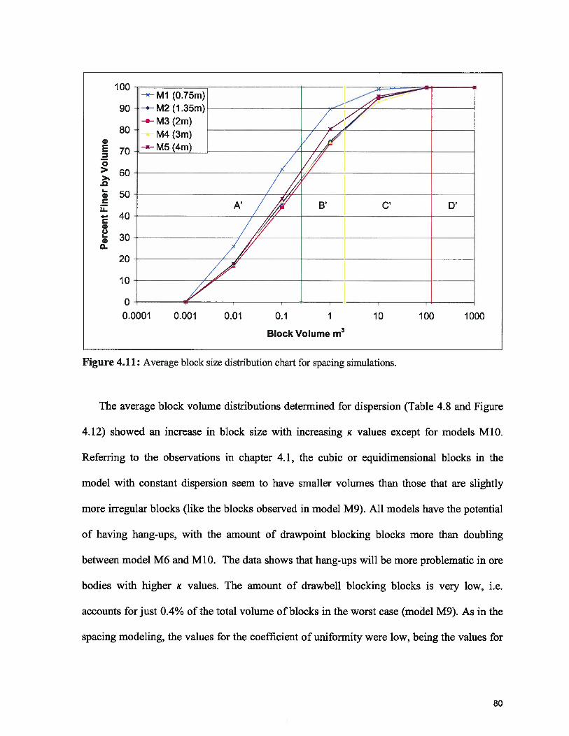
-Ml (O.75m)—i-- M2 (1 .35m)-.-M3(2m)

M4(3m)M5(4m)

.________

//7

A’ // B’ C’ D’

/,/1

Figure 4.11: Average block size distribution chart for spacing simulations.

The average block volume distributions determined for dispersion (Table 4.8 and Figure

4.12) showed an increase in block size with increasing K values except for models M1O.

Referring to the observations in chapter 4.1, the cubic or equidimensional blocks in the

model with constant dispersion seem to have smaller volumes than those that are slightly

more irregular blocks (like the blocks observed in model M9). All models have the potential

of having hang-ups, with the amount of drawpoint blocking blocks more than doubling

between model M6 and Mb. The data shows that hang-ups will be more problematic in ore

bodies with higher ic values. The amount of drawbell blocking blocks is very low, i.e.

accounts for just 0.4% of the total volume of blocks in the worst case (model M9). As in the

spacing modeling, the values for the coefficient of uniformity were low, being the values for

100

90

80

70

____________ __________ ___

>60>1

.0

G) 50LI40

0.0001 0.001 0.01 0.1 1 10 100 1000

Block Volume m3

80

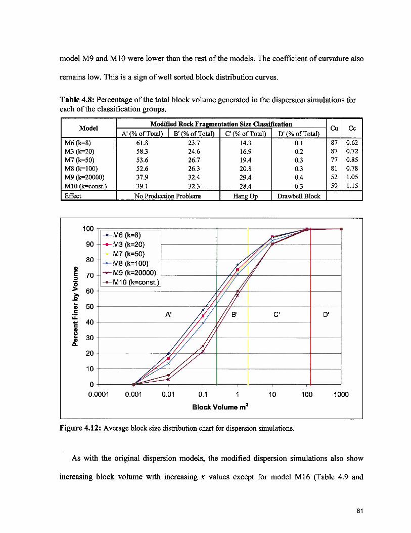
model M9 and M1O were lower than the rest of the models. The coefficient of curvature also

remains low. This is a sign of well sorted block distribution curves.

Table 4.8: Percentage of the total block volume generated in the dispersion simulations foreach of the classification groups.

Modified Rock Fragmentation Size ClassificationModel Cu Cc

A’ (% of Total) B’ (% of Total) C’ (% of Total) D’ (% of Total) —

M6 (k=8) 61.8 23.7 14.3 0.1 87 0.62M3 (k=20) 58.3 24.6 16.9 0.2 87 0.72M7 (k=50) 53.6 26.7 19.4 0.3 77 0.85M8 (k=100) 52.6 26.3 20.8 0.3 81 0.78M9 (k=20000) 37.9 32.4 29.4 0.4 52 1.05

Ml0 (k=const.) 39.1 32.3 28.4 0.3 59 1.15

Effect No Production Problems Hang Up Drawbell Block

100•—.— M6 (k=8)

90 — M3 (k=20)M7 (k=50)

,;80 -M8 (k=100)

CI

70 —*— M9 (k=20000)-.—M10 (k=const.)

60 //.

//B1 C’ D’40.CI

30

I

Il

0

20

10

00.0001 0.001 0.01 0.1 1 10 100 1000

Block Volume m3

Figure 4.12: Average block size distribution chart for dispersion simulations.

As with the original dispersion models, the modified dispersion simulations also show

increasing block volume with increasing K values except for model M16 (Table 4.9 and

81

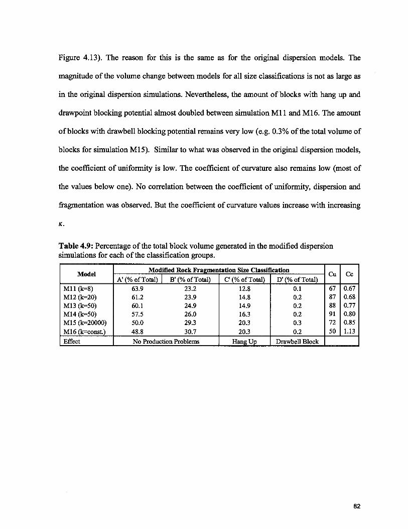
Figure 4.13). The reason for this is the same as for the original dispersion models. The

magnitude of the volume change between models for all size classifications is not as large as

in the original dispersion simulations. Nevertheless, the amount of blocks with hang up and

drawpoint blocking potential almost doubled between simulation Ml 1 and M16. The amount

of blocks with drawbell blocking potential remains very low (e.g. 0.3% of the total volume of

blocks for simulation M15). Similar to what was observed in the original dispersion models,

the coefficient of uniformity is low. The coefficient of curvature also remains low (most of

the values below one). No correlation between the coefficient of uniformity, dispersion and

fragmentation was observed. But the coefficient of curvature values increase with increasing

K.

Table 4.9: Percentage of the total block volume generated in the modified dispersionsimulations for each of the classification groups.

Modified Rock Fragmentation Size ClassificationModel Cu Cc

A’ (% of Total) B’ (% of Total) C’ (% of Total) D’ (% of Total) — —

Mu (k=8) 63.9 23.2 12.8 0.1 67 0.67M12 (k=20) 61.2 23.9 14.8 0.2 87 0.68M13 (k=50) 60.1 24.9 14.9 0.2 88 0.77M14 (k=50) 57.5 26.0 16.3 0.2 91 0.80M15 (k=20000) 50.0 29.3 20.3 0.3 72 0.85

M16 (k=const.) 48.8 30.7 20.3 0.2 50 1.13

Effect No Production Problems Hang Up Drawbell Block

82

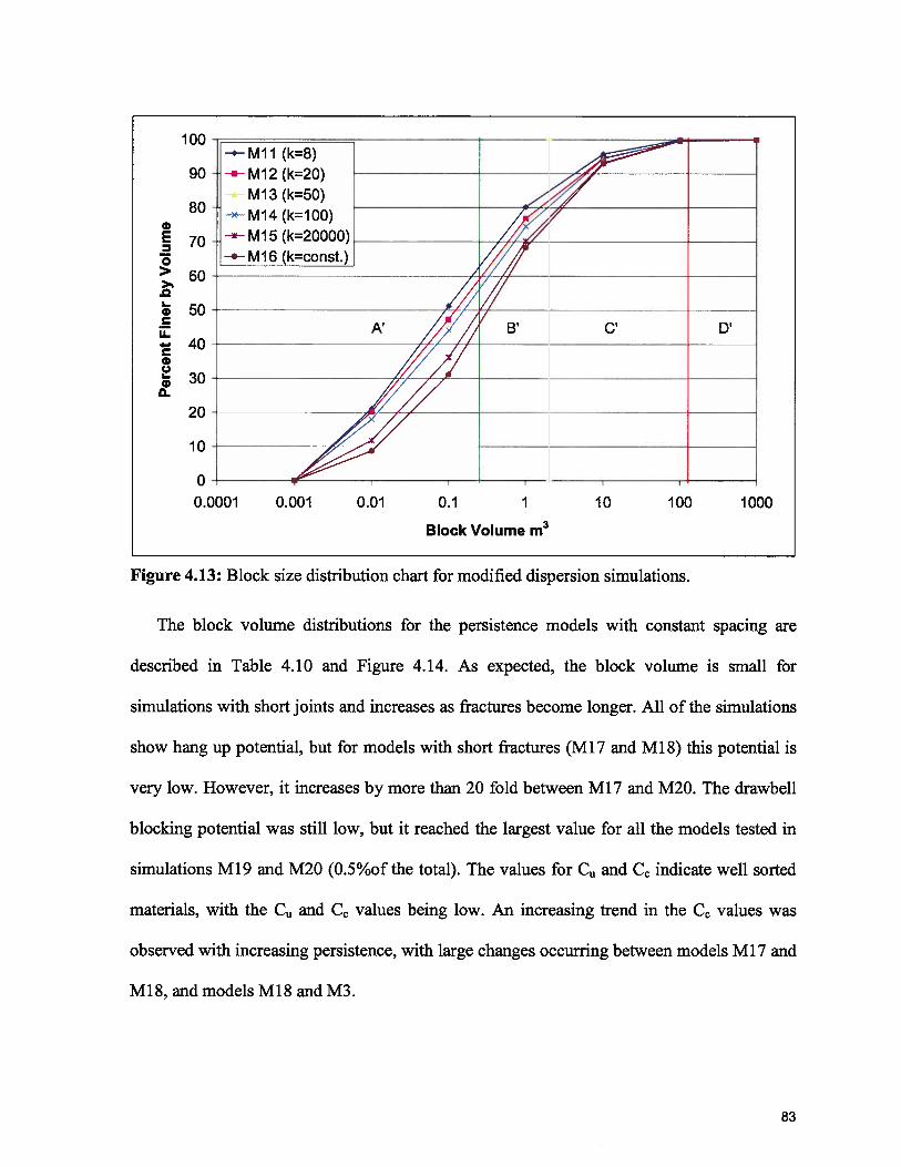
-.--M11 (k=8)-.-M12(k=20)

M13 (k=50)-—M14(k=lOO)

C.

-*—M15 (k=20000)-.— M16 (k=const.)

A’ B’ C’ D’

////

Figure 4.13: Block size distribution chart for modified dispersion simulations.

The block volume distributions for the persistence models with constant spacing are

described in Table 4.10 and Figure 4.14. As expected, the block volume is small for

simulations with short joints and increases as fractures become longer. All of the simulations

show hang up potential, but for models with short fractures (M17 and M18) this potential is

very low. However, it increases by more than 20 fold between M17 and M20. The drawbell

blocking potential was still low, but it reached the largest value for all the models tested in

simulations M19 and M20 (0.5%of the total). The values for C and C indicate well sorted

materials, with the C and C values being low. An increasing trend in the C values was

observed with increasing persistence, with large changes occurring between models M17 and

M18, and models M18 and M3.

100

90

80

>60.0I-a 50

40

I-a)0

20

10

00.0001 0.001 0.01 0.1 1

Block Volume m3

10 100 1000

83

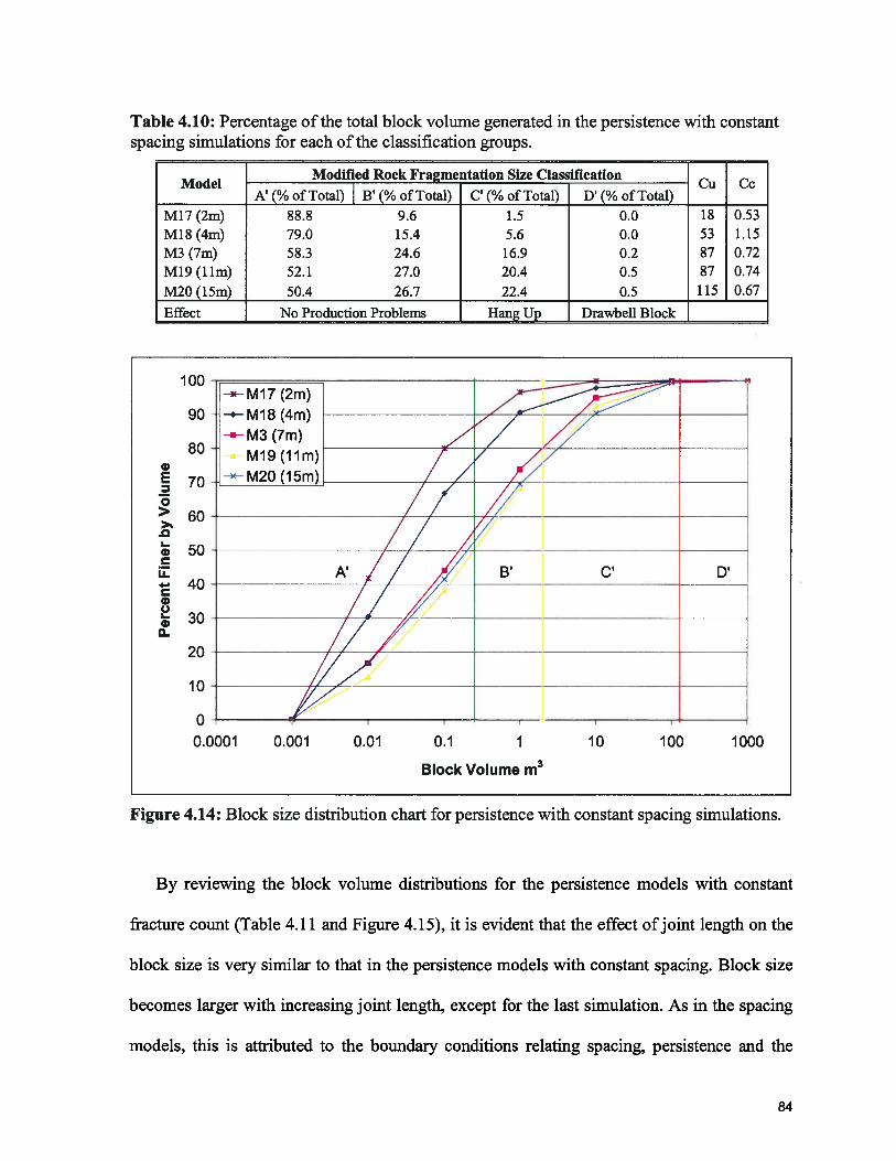
Table 4.10: Percentage of the total block volume generated in the persistence with constantspacing simulations for each of the classification groups.

Modified Rock Fragmentation Size ClassificationModel Cu Cc

A’ (% of Total) B’ (% of Total) C’ (% of Total) D’ (% of Total) —

M17 (2m) 88.8 9.6 1.5 0.0 18 0.53M18 (4m) 79.0 15.4 5.6 0.0 53 1.15M3 (7m) 58.3 24.6 16.9 0.2 87 0.72M19(llm) 52.1 27.0 20.4 0.5 87 0.74

M20(15m) 50.4 26.7 22.4 0.5 115 0.67

Effect No Production Problems Hang Up Drawbell Block

w Ml 7 (2m)

:=M19(llm) / / //

--M20(15m) / /Z

B’

C’ D’

Figure 4.14: Block size distribution chart for persistence with constant spacing simulations.

By reviewing the block volume distributions for the persistence models with constant

fracture count (Table 4.11 and Figure 4.15), it is evident that the effect ofjoint length on the

block size is very similar to that in the persistence models with constant spacing. Block size

becomes larger with increasing joint length, except for the last simulation. As in the spacing

models, this is attributed to the boundary conditions relating spacing, persistence and the

100

90

80

70

>60

G 50LI40C.)I

0

20

10

0

0.0001 0.001 0.01 0.1 1

Block Volume m3

10 100 1000

84

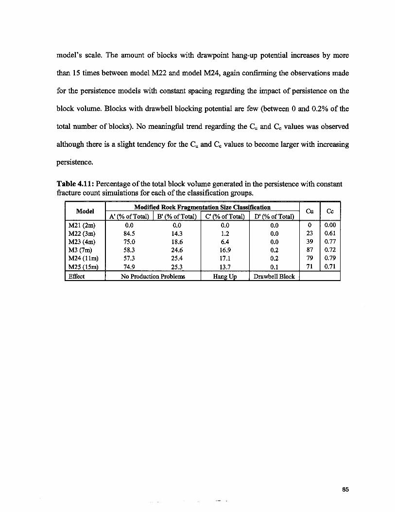
model’s scale. The amount of blocks with drawpoint hang-up potential increases by more

than 15 times between model M22 and model M24, again confiniiing the observations made

for the persistence models with constant spacing regarding the impact of persistence on the

block volume. Blocks with drawbell blocking potential are few (between 0 and 0.2% of the

total number of blocks). No meaningful trend regarding the C and C values was observed

although there is a slight tendency for the C and C values to become larger with increasing

persistence.

Table 4.11: Percentage of the total block volume generated in the persistence with constantfracture count simulations for each of the classification groups.

Modified Rock Fragmentation Size ClassificationModel Cu Cc

A’ (% of Total) B’ (% of Total) C? (% of Total) D’ (% of Total)

M21 (2m) 0.0 0.0 0.0 0.0 0 0.00M22 (3m) 84.5 14.3 1.2 0.0 23 0.61M23 (4m) 75.0 18.6 6.4 0.0 39 0.77M3 (7m) 58.3 24.6 16.9 0.2 87 0.72M24(llm) 57.3 25.4 17.1 0.2 79 0.79

M25 (15m) 74.9 25.3 13.7 0.1 71 0.71

Effect No Production Problems Hang Up Drawbell Block

85

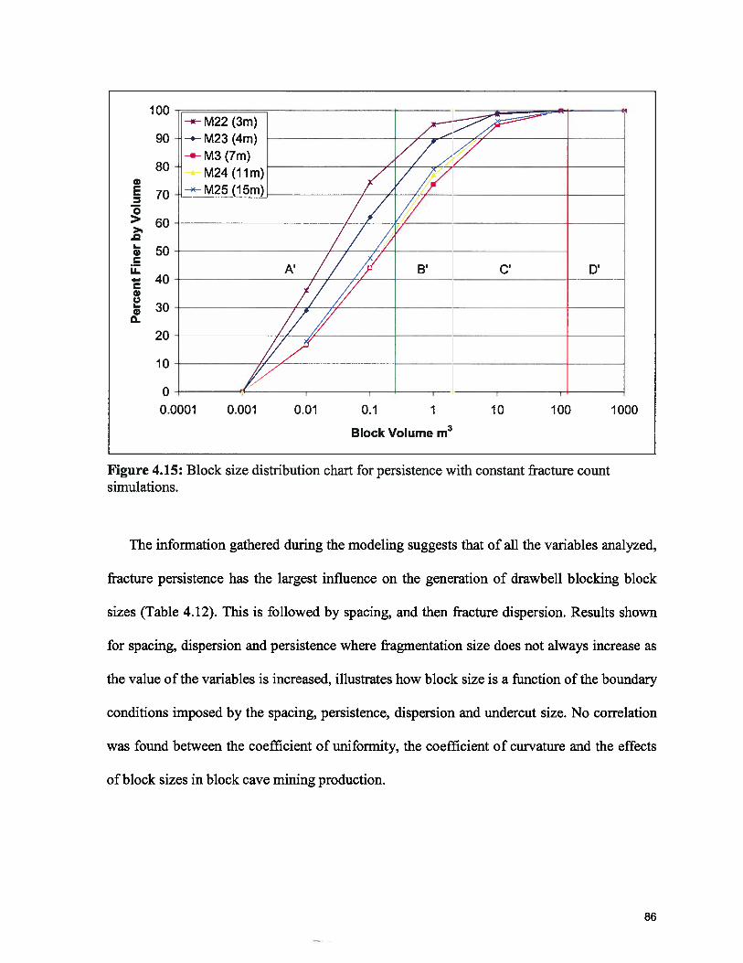
-*-- M22 (3m)-.--M23(4m)—.--M3(7m)

--M25 (15m)M24(llm)

A’ B’ C’ D’

j/

*k

Figure 4.15: Block size distribution chart for persistence with constant fracture countsimulations.

The information gathered during the modeling suggests that of all the variables analyzed,

fracture persistence has the largest influence on the generation of drawbell blocking block

sizes (Table 4.12). This is followed by spacing, and then fracture dispersion. Results shown

for spacing, dispersion and persistence where fragmentation size does not always increase as

the value of the variables is increased, illustrates how block size is a function of the boundary

conditions imposed by the spacing, persistence, dispersion and undercut size. No correlation

was found between the coefficient of uniformity, the coefficient of curvature and the effects

of block sizes in block cave mining production.

100

90

80

i70

>60

I-a, 50

40a)0I-a)0.

20

10

00.0001 0.001 0.01 0.1 1

Block Volume m3

10 100 1000

86

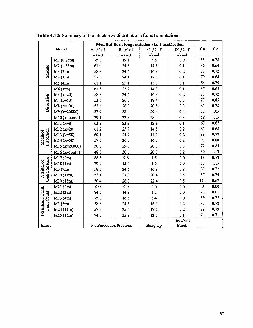
Table 4.12: Summary of the block size distributions for all simulations.

Modified Rock Fragmentation Size ClassificationModel A’ (% of B’ (% of C’ (% of D’ (% of Cu Cc

Total) Total) Total) Total)

Ml (0.75m) 75.0 19.1 5.8 0.0 38 0.78

M2 (1.35m) 61.0 24.3 14.6 0.1 86 0.64

M3 (2m) 58.3 24.6 16.9 0.2 87 0.72

M4 (3m) 57.7 24.1 18.1 0.1 79 0.64

M5 (4m) 61.1 25.1 13.7 0.1 64 0.70

M6 (k=8) 61.8 23.7 14.3 0.1 87 0.62

M3 (k=20) 58.3 24.6 16.9 0.2 87 0.72

1 M7 (k=50) 53.6 26.7 19.4 0.3 77 0.85

M8 (k=100) 52.6 26.3 20.8 0.3 81 0.78

M9 (k=20000) 37.9 32.4 29.4 0.4 52 1.05

M10 (k=const.) 39.1 32.3 28.4 0.3 59 1.15

Mu (k=8) 63.9 23.2 12.8 0.1 67 0.67

.M12 (k=20) 61.2 23.9 14.8 0.2 87 0.68

I M13 (k=50) 60.1 24.9 14.9 0.2 88 0.77. Q

M14 (k=50) 57.5 26.0 16.3 0.2 91 0.80

M15 (lc=20000) 50.0 29.3 20.3 0.3 72 0.85

M16 (k=const.) 48.8 30.7 20.3 0.2 50 1.13

M17 (2m) 88.8 9.6 1.5 0.0 18 0.53

M18 (4m) 79.0 15.4 5.6 0.0 53 1.15

.M3 (7m) 58.3 24.6 16.9 0.2 87 0.72

M19(llm) 52.1 27.0 20.4 0.5 87 0.74

M20 (15m) 50.4 26.7 22.4 0.5 115 0.67

. M21 (2m) 0.0 0.0 0.0 0.0 0 0.00

M22 (3m) 84.5 14.3 1.2 0.0 23 0.61

M23 (4m) 75.0 18.6 6.4 0.0 39 0.77

,

M3 (7m) 58.3 24.6 16.9 0.2 87 0.72

M24(llm) 57.3 25.4 17.1 0.2 79 0.79

M25(15m) 74.9 25.3 13.7 0.1 71 0.71Drawbell

Effect No Production Problems Hang Up Block

87

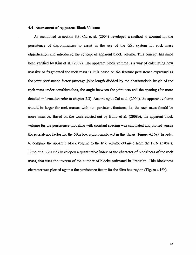
4.4 Assessment of Apparent Block Volume

As mentioned in section 3.3, Cai et al. (2004) developed a method to account for the

persistence of discontinuities to assist in the use of the GSI system for rock mass

classification and introduced the concept of apparent block volume. This concept has since

been verified by Kim et al. (2007). The apparent block volume is a way of calculating how

massive or fragmented the rock mass is. It is based on the fracture persistence expressed as

the joint persistence factor (average joint length divided by the characteristic length of the

rock mass under consideration), the angle between the joint sets and the spacing (for more

detailed information refer to chapter 2.3). According to Cai et al. (2004), the apparent volume

should be larger for rock masses with non persistent fractures, i.e. the rock mass should be

more massive. Based on the work carried out by Elmo et al. (2008b), the apparent block

volume for the persistence modeling with constant spacing was calculated and plotted versus

the persistence factor for the 50m box region employed in this thesis (Figure 4.1 6a). In order

to compare the apparent block volume to the true volume obtained from the DFN analysis,

Elmo et al. (2008b) developed a quantitative index of the character of blockiness of the rock

mass, that uses the inverse of the number of blocks estimated in FracMan. This blockiness

character was plotted against the persistence factor for the 50m box region (Figure 4.1 6b).

88

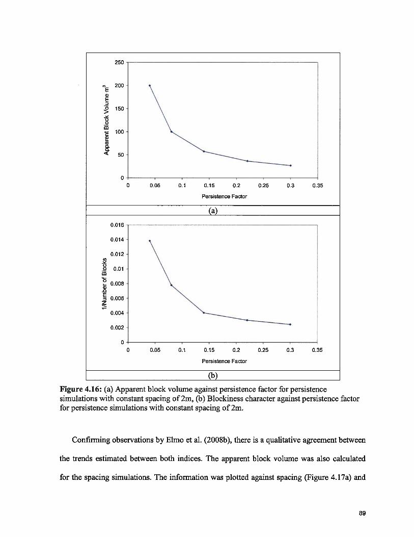
250

c)Eci)E

the trends estimated between both indices. The apparent block volume was also calculated

for the spacing simulations. The information was plotted against spacing (Figure 4.17a) and

200

150

100

50

00 0.05 0.1 0.15 0.2 0.25 0.3 0.35

Persistence Factor

(a)

0

C)0

ci)

z

0.016

0.014

0.012

0.01

0.008

0.006

0.004

0.002

00 0.05 0.1 0.15 0.2 0.25 0.3 0.35

Persistence Factor

(b)

Figure 4.16: (a) Apparent block volume against persistence factor for persistencesimulations with constant spacing of 2m, (b) Blockiness character against persistence factorfor persistence simulations with constant spacing of 2m.

Confirming observations by Elmo et al. (2008b), there is a qualitative agreement between

89

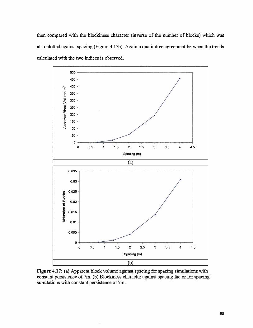
then compared with the blockiness character (inverse of the number of blocks) which was

also plotted against spacing (Figure 4.17b). Again a qualitative agreement between the trends

calculated with the two indices is observed.

500

450

) 400E

350

300

250

200

150

100

50

0

0 0.5 1 1.5 2 2.5 3 3.5 4 4.5

Spacing (m)

(b)

Figure 4.17: (a) Apparent block volume against spacing for spacing simulations withconstant persistence of 7m, (b) Blockiness character against spacing factor for spacingsimulations with constant persistence of 7m.

0 0.5 1 1.5 2 2.5 3 3.5 4 4.5

Spacing (m)

(a)

C)0

.0E

z

0.035

0.03

0.025

0.02

0.015

0.01

0.005

0

90

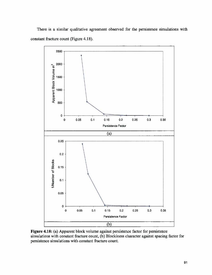
There is a similar qualitative agreement observed for the persistence simulations with

Ci,

00

0

a).0E

z

2500

1500

500

0

0.25

0.2

0.15

0.1

0.05

0

(a)

(b)

Figure 4.18: (a) Apparent block volume against persistence factor for persistencesimulations with constant fracture count, (b) Blockiness character against spacing factor forpersistence simulations with constant fracture count.

constant fracture count (Figure 4.18).

, 2000Ea)

0>00

1000

Co00.

0 0.05 0.1 0.15 0.2 0.25 0.3 0.35

Persistence Factor

0 0.05 0.1 0.15 0.2 0.25 0.3 0.35

Persistence Factor

91

The dispersion simulations were again plotted against the persistence factor, however in

this case no agreement between the apparent block volume and the blockiness character was

observed (Figure 4.19 Figure 4.20) In Figures 4.1 9a and 4.20a, all values are concentrated at

one point because the apparent volume does not take into consideration dispersion. As

observed in Figure 4.1 9b and 4.20b, dispersion has an effect in the blockiness of the

rockmass; the blockiness character increasing with increasing K.

92

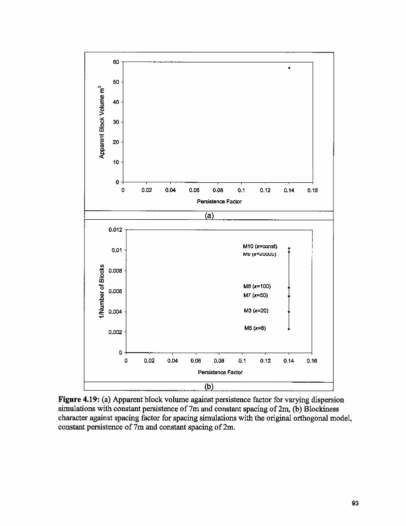
60

50

E

40

30

20CD

0.

10

00 0.02 0.04 0.06 0.08 0.1 0.12 0.14 0.16

Persistence Factor

(a)

0.012

0.01M10 (K=const)M K2UUUU)

0

00

M8(K100)0.006

M7 (x50)

2z o.oo M3 (x20)

M6 (,c8)0.002

0

0 0.02 0.04 0.06 0.08 0.1 0.12 0.14 0.16

Persistence Factor

(b)

Figure 4.19: (a) Apparent block volume against persistence factor for varying dispersionsimulations with constant persistence of 7m and constant spacing of 2m, (b) Blockinesscharacter against spacing factor for spacing simulations with the original orthogonal model,constant persistence of 7m and constant spacing of 2m.

93

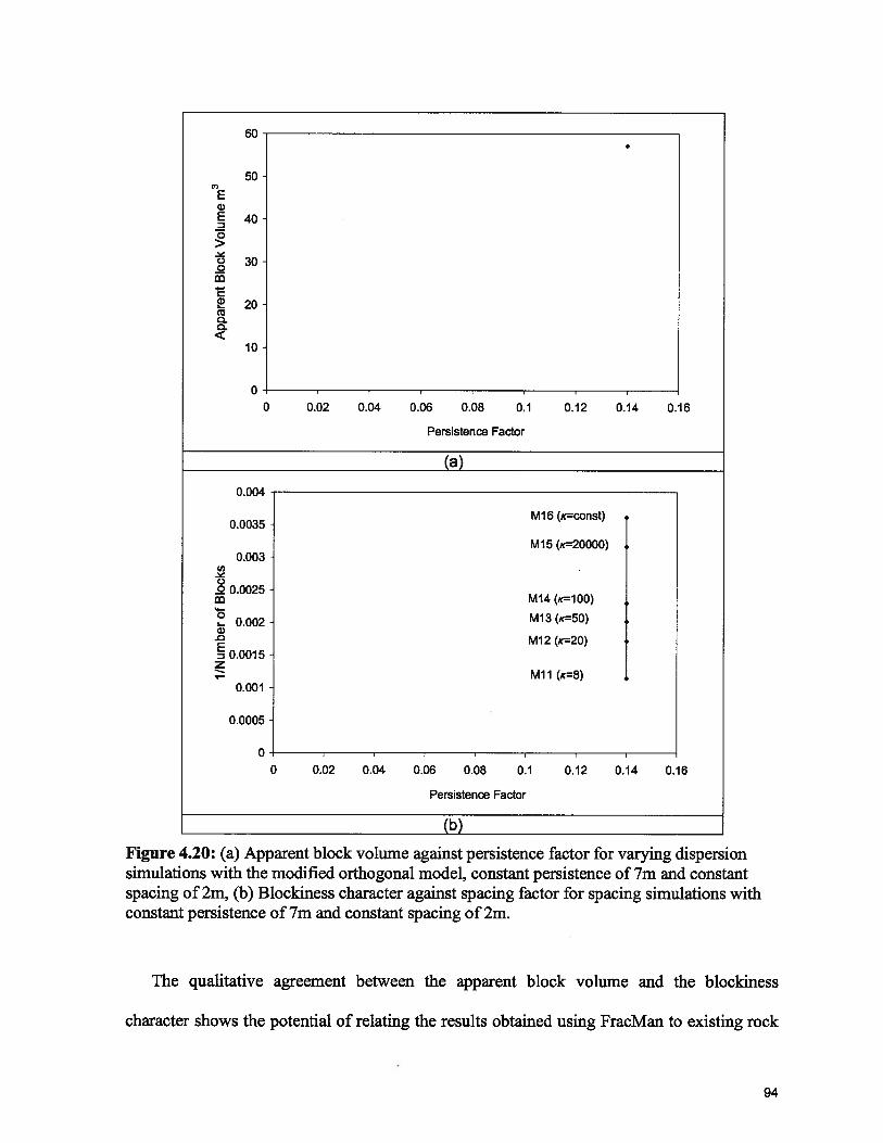
60.

50C.,

E

40

30

20

10

0 I

0 0.02 0.04 0.06 0.08 0.1 0.12 0.14 0.16

Persistence Factor

(a)

0.004

Ml 6 (Kconst)0.0035

M15 (K=20000)0.003

0

0.2 0.0025

M14fr100)

0.002 M13(K=50)

M12(x20)D 0.0015z

Mu (K8)0.001

0.0005

0

0 0.02 0.04 0.06 0.08 0.1 0.12 0.14 0.16

Persistence Factor

(b)

Figure 4.20: (a) Apparent block volume against persistence factor for varying dispersionsimulations with the modified orthogonal model, constant persistence of 7m and constantspacing of 2m, (b) Blockiness character against spacing factor for spacing simulations withconstant persistence of 7m and constant spacing of 2m.

The qualitative agreement between the apparent block volume and the blockiness

character shows the potential of relating the results obtained using FracMan to existing rock

94

mass classification systems. However, the apparent block volume needs to be modified to

incorporate the effect of fracture dispersion.

4.5 Block Trace Areas and Block Volumes for Generated Models

Comparing the block trace areas on the undercut and block volumes generated can be

used to assess the influence on the initial caveability potential of each of the tested variables.

To compare the models, the block areas on the undercut were normalized against the total

area of the undercut. The volume of blocks generated was also normalized, but to the volume

of the ore body or “inner box” (defined in Section 3.1.2.) and expressed as a percentage (%)

of total ore body volume. FracMan does not consider the propagation of the cave, so this

investigation only relates to the initial stage of caving (i.e. the opening of the undercut). The

following parameters were used in the analysis:

1. The total block area — this is the total area of the blocks generated as seen from below

the undercut (Figure 4.21);

2. The total unstable block area — this is the area of all blocks with a factor of safety less

than one seen in the undercut, i.e. the area on the undercut of the “key blocks” using

Goodman and Shi’s (1985) classification scheme. Key blocks are important because

their removal can trigger the mobilization of stable blocks;

95

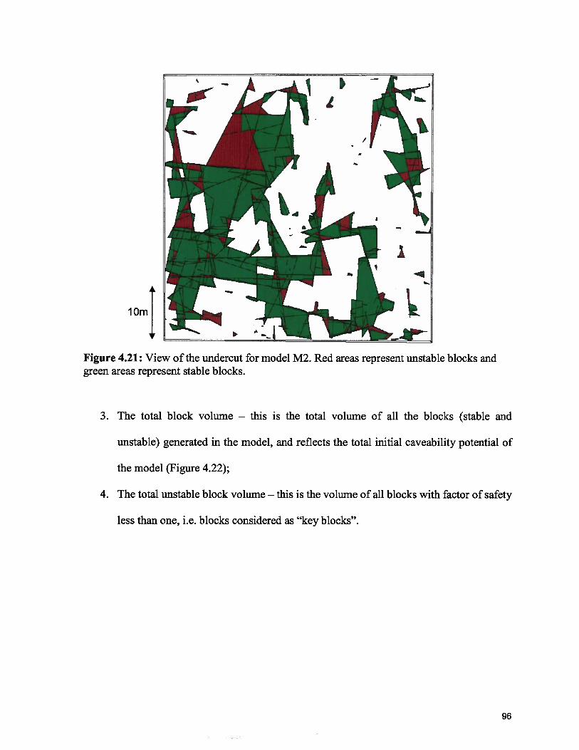
lOm

—

__

Figure 4.21: View of the undercut for model M2. Red areas represent unstable blocks andgreen areas represent stable blocks.

3. The total block volume — this is the total volume of all the blocks (stable and

unstable) generated in the model, and reflects the total initial caveability potential of

the model (Figure 4.22);

4. The total unstable block volume — this is the volume of all blocks with factor of safety

less than one, i.e. blocks considered as “key blocks”.

‘bJ

96

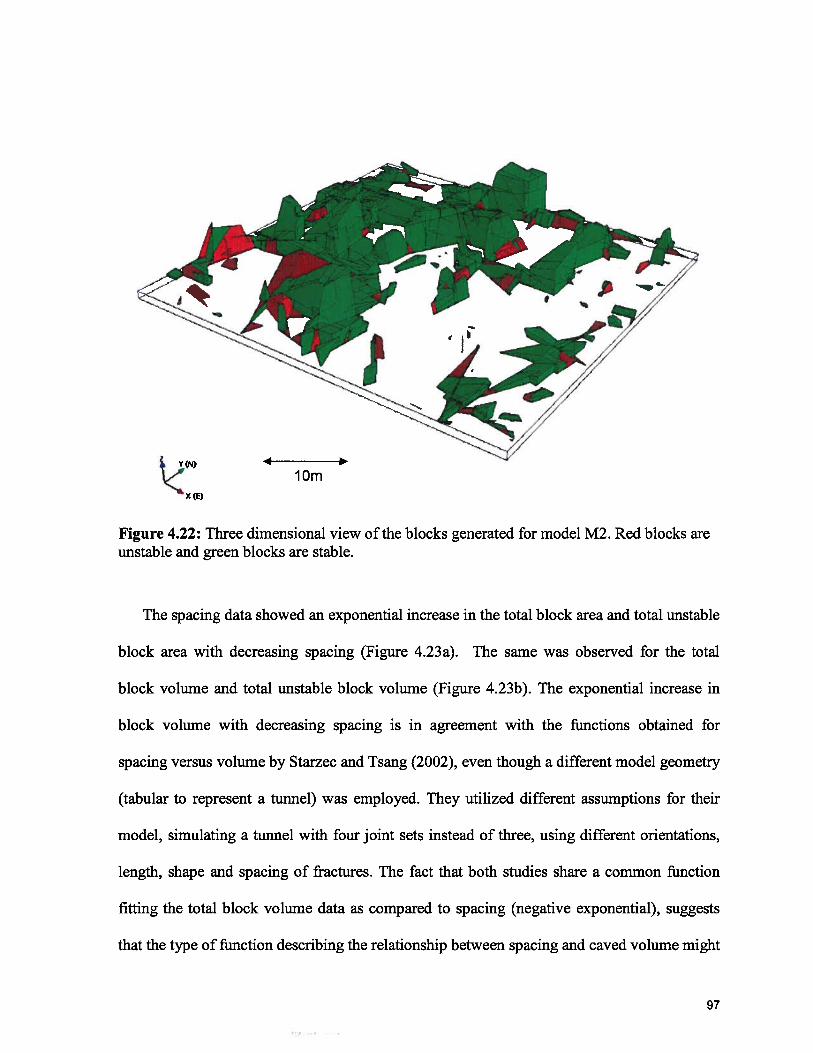
) (t)

•0 ‘7

Figure 4.22: Three dimensional view of the blocks generated for model M2. Red blocks areunstable and green blocks are stable.

The spacing data showed an exponential increase in the total block area and total unstable

block area with decreasing spacing (Figure 4.23a). The same was observed for the total

block volume and total unstable block volume (Figure 4.23b). The exponential increase in

block volume with decreasing spacing is in agreement with the functions obtained for

spacing versus volume by Starzec and Tsang (2002), even though a different model geometry

(tabular to represent a tunnel) was employed. They utilized different assumptions for their

model, simulating a tunnel with four joint sets instead of three, using different orientations,

length, shape and spacing of fractures. The fact that both studies share a common function

fitting the total block volume data as compared to spacing (negative exponential), suggests

that the type of function describing the relationship between spacing and caved volume might

r7

//

—

—-4...4 I’1 Om

97

be independent of the number of joint sets, the orientation of the sets, length, shape and

spacing of fractures, and the geometry of the free face. In the case of a comparison between

spacing and area, and spacing and volume the function describing the relationship will be a

negative exponential curve, as long as the fractures are randomly distributed in space

(Poisson process). In the case of these models (Starzec and Tsang’s and the models in this

thesis) this applies, since they were simulated using the Enhanced Baecher model. As

described in Chapter 4, the Enhanced Baecher model follows a 3D Poisson process, and the

probability density function of a Poisson process is a negative exponential function.

98

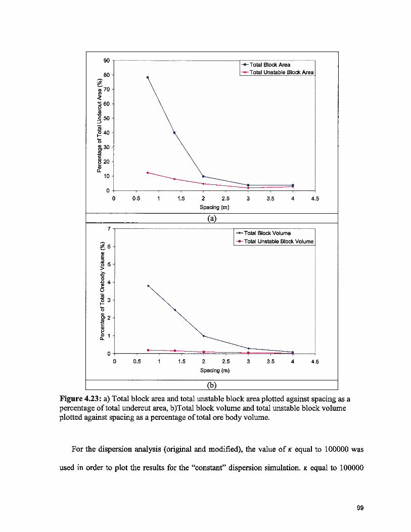
-.— Total Block Area

80 -.— Total Unstable Block Area

c 70a)

600

50

30

C

0a)0

10

0 I

O 0.5 1 1.5 2 2.5 3 3.5 4 4.5

Spacing (m)

(a)7

--- Total Block Volume

-.— Total Unstable Block Volume

a)2Do5>>

0.04G)

0

g’2C

0

0 0.5 1 1.5 2 2.5 3 3.5 4 4.5

Spacing (m)

(b)

Figure 4.23: a) Total block area and total unstable block area plotted against spacing as apercentage of total undercut area, b)Total block volume and total unstable block volumeplotted against spacing as a percentage of total ore body volume.

For the dispersion analysis (original and modified), the value of K equal to 100000 was

used in order to plot the results for the “constant” dispersion simulation. K equal to 100000

99

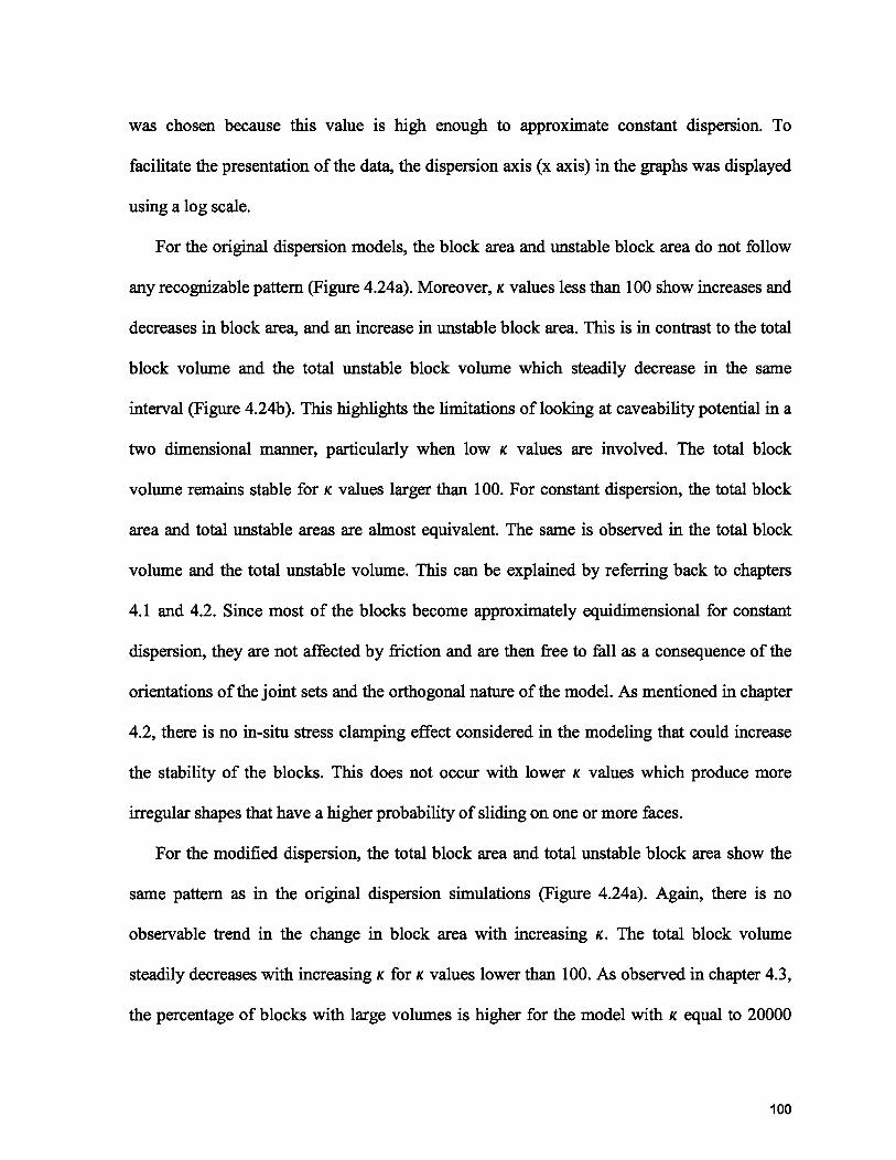
was chosen because this value is high enough to approximate constant dispersion. To

facilitate the presentation of the data, the dispersion axis (x axis) in the graphs was displayed

using a log scale.

For the original dispersion models, the block area and unstable block area do not follow

any recognizable pattern (Figure 4.24a). Moreover, K values less than 100 show increases and

decreases in block area, and an increase in unstable block area. This is in contrast to the total

block volume and the total unstable block volume which steadily decrease in the same

interval (Figure 4.24b). This highlights the limitations of looking at caveability potential in a

two dimensional manner, particularly when low K values are involved. The total block

volume remains stable for K values larger than 100. For constant dispersion, the total block

area and total unstable areas are almost equivalent. The same is observed in the total block

volume and the total unstable volume. This can be explained by referring back to chapters

4.1 and 4.2. Since most of the blocks become approximately equidimensional for constant

dispersion, they are not affected by friction and are then free to fall as a consequence of the

orientations of the joint sets and the orthogonal nature of the model. As mentioned in chapter

4.2, there is no in-situ stress clamping effect considered in the modeling that could increase

the stability of the blocks. This does not occur with lower K values which produce more

irregular shapes that have a higher probability of sliding on one or more faces.

For the modified dispersion, the total block area and total unstable block area show the

same pattern as in the original dispersion simulations (Figure 4.24a). Again, there is no

observable trend in the change in block area with increasing K. The total block volume

steadily decreases with increasing K for K values lower than 100. As observed in chapter 4.3,

the percentage of blocks with large volumes is higher for the model with K equal to 20000

100

than for the model with constant dispersion. This is reflected in the total block volume in

which the same trend is seen. The unstable block volume follows a very similar trend to the

original dispersion modeling, remaining approximately at the same value for all the

simulations except for the model with constant dispersion. With constant dispersion the total

unstable block volume does not become as large a percentage of the total block volume as in

the dispersion simulations. This is attributed to the different orientation of two of the joint

sets which allows for the formation of tapered and potential key blocks.

101

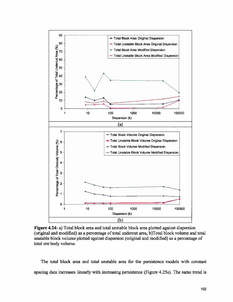
90-.— Total Block Area Original Dispersion

80 -“--Total Unstable Block Area Original Dispersion

70 —a— Total Block Area Modified Dispersion

— Total Unstable Block Area Modified Dispersion60

a)50

1 10 100 1000 10000 100000

Dispersion (k)

(a)

7—‘—Total Block Volume Original Dispersion

2 6 —Total Unstable Block Volume Original Dispersion

-—Total Block Volume Modified Dispersion

5 —Total Unstable Block Volume Modified Dispersion>>‘.

1 10 100 1000 10000 100000

Dispersion (k)

(b)

Figure 4.24: a) Total block area and total unstable block area plotted against dispersion(original and modified) as a percentage of total undercut area, b)Total block volume and totalunstable block volume plotted against dispersion (original and modified) as a percentage oftotal ore body volume.

The total block area and total unstable area for the persistence models with constant

spacing data increases linearly with increasing persistence (Figure 4.25a). The same trend is

102

observed for the total block volume and unstable block volume (Figure 4.25b). When

comparing the generation of block areas and block volumes for a certain fracture length,

significant block areas (greater than 5%) are generated for relatively short fractures (4m). But

for a 4m fracture length there is very little total volume produced. This shows again the

limitations of using a two dimensional analysis (the block area) to describe a three

dimensional process (caveability).

103

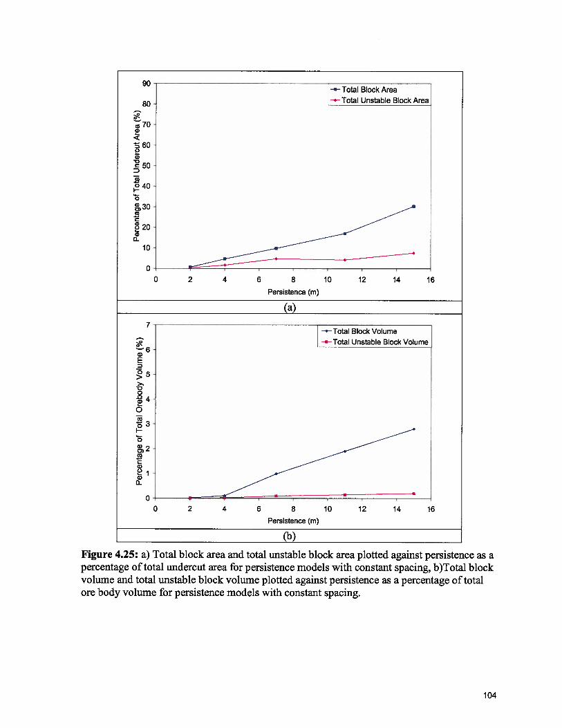
90

80

;-70Co

60C-)

Co

50

40

0

30Co

CoC) 20

a-10

0

7

I:0CO

0I9-0a)COC0)

0)a-

0

0 2 4 6 8 10 12 14 16

Persistence (m)

(a)

(b)

Figure 4.25: a) Total block area and total unstable block area plotted against persistence as apercentage of total undercut area for persistence models with constant spacing, b)Total blockvolume and total unstable block volume plotted against persistence as a percentage of totalore body volume for persistence models with constant spacing.

-Total Block Area-.— Total Unstable Block Area

0 2 4 6 8 10 12 14 16

Persistence (m)

104

In the persistence models with constant fracture count the total block and unstable block

area increase linearly with increasing persistence (Figure 4.26a). The total block volume and

total unstable block volume follow similar trends also increasing linearly with increasing

persistence (Figure 4.26b). In these simulations fractures were generated until a specified

number was reached. No spacing was assigned and persistence alone was changed. These

conditions indirectly modified the spacing of each of the models. If the ore bodies were to be

surveyed for spacing, it would be observed that the changes in persistence lead to a change in

fracture spacing. A decrease in spacing related to an increase in joint persistence would be

detected, due to the fact that longer fractures have a higher probability of intersecting a

borehole or a wall than short fractures. The fracture spacing for all the persistence models

with constant fracture count was calculated from measurements in the predefined boreholes

in the model. For the models with joint persistence of 2, 3 and 4m the spacing is 9.4, 5.2 and

3.5m respectively. These values correlate with the results for the spacing modeling in Figure

4.23b. This may explain the differences between the persistence models with constant

spacing and the persistence models with constant fracture count.

105

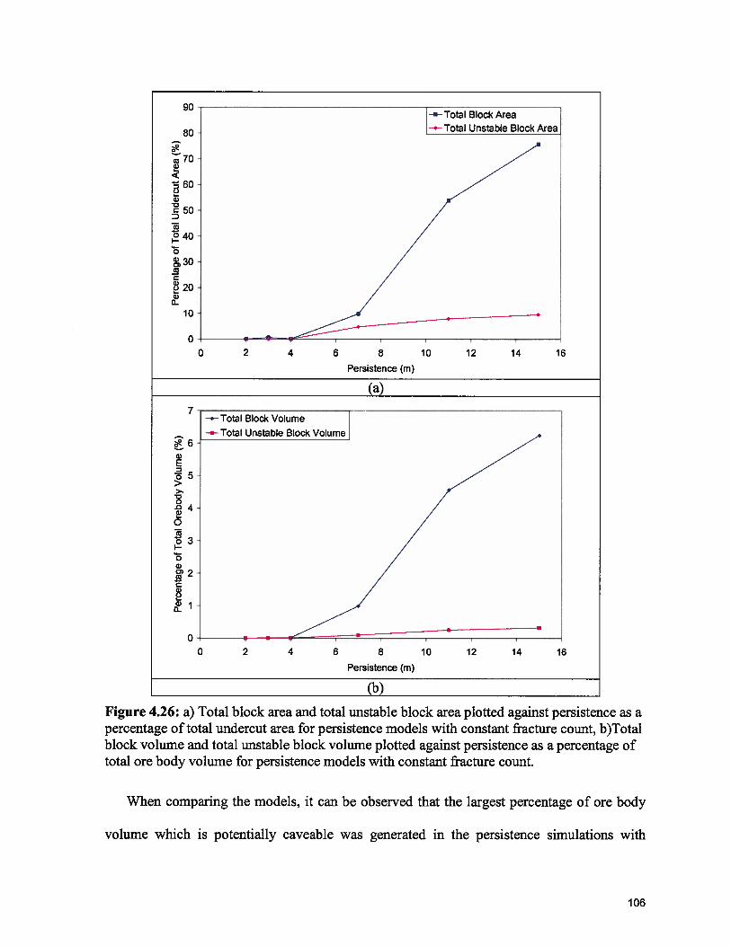
90

;70

60C.)

50

12400

30

a)o 20a)

U-

10

7

a)2

>>

0.0a)

0

0I—

0a)

C

a)

0

4

3

I

(a)

(b)

10 12 14 16

Figure 4.26: a) Total block area and total unstable block area plotted against persistence as apercentage of total undercut area for persistence models with constant fracture count, b)Totalblock volume and total unstable block volume plotted against persistence as a percentage oftotal ore body volume for persistence models with constant fracture count.

When comparing the models, it can be observed that the largest percentage of ore body

volume which is potentially caveable was generated in the persistence simulations with

80

0

0 2 4 6 8 10 12 14 16

Persistence (m)

0 2 4 6 8

Persistence (m)

106

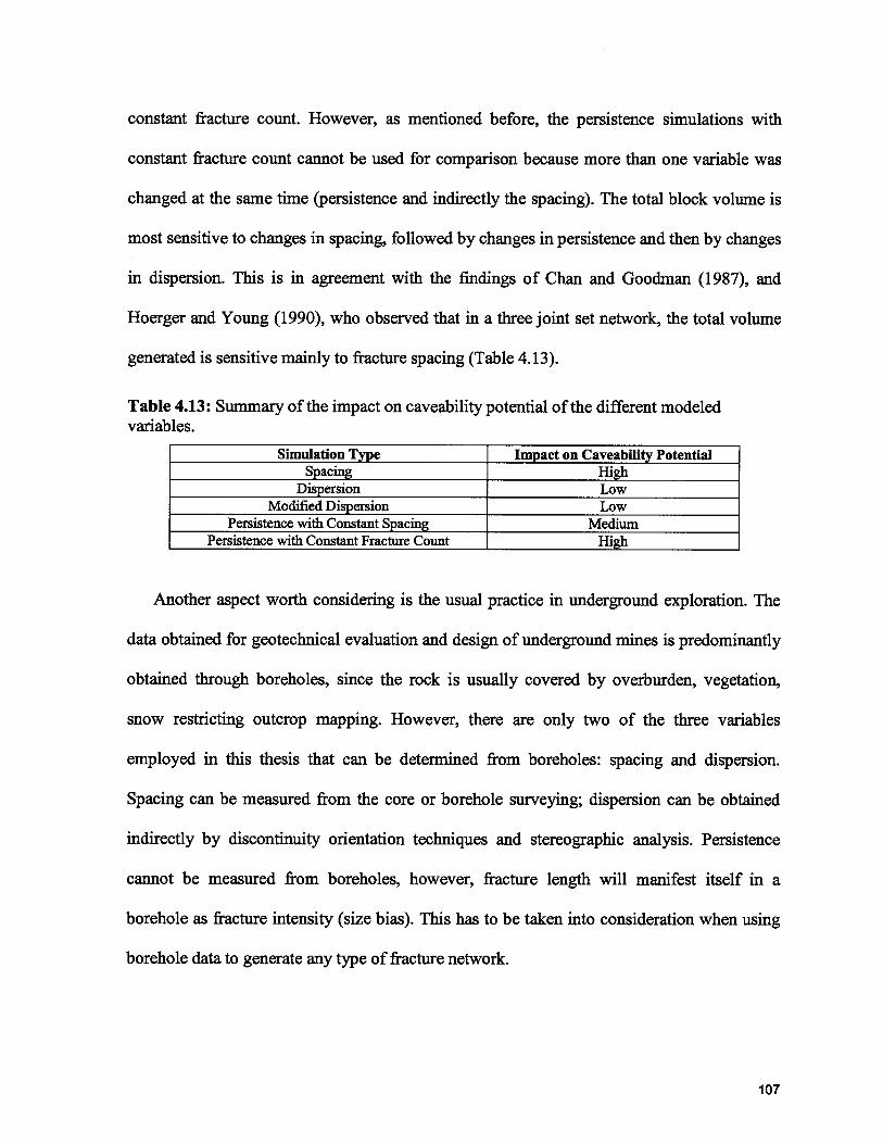
constant fracture count. However, as mentioned before, the persistence simulations with

constant fracture count cannot be used for comparison because more than one variable was

changed at the same time (persistence and indirectly the spacing). The total block volume is

most sensitive to changes in spacing, followed by changes in persistence and then by changes

in dispersion. This is in agreement with the findings of Chan and Goodman (1987), and

Hoerger and Young (1990), who observed that in a three joint set network, the total volume

generated is sensitive mainly to fracture spacing (Table 4.13).

Table 4.13: Summary of the impact on caveability potential of the different modeledvariables.

Simulation Type Impact on Caveability PotentialSpacing High

Dispersion LowModified Dispersion Low

Persistence with Constant Spacing MediumPersistence with Constant Fracture Count High

Another aspect worth considering is the usual practice in underground exploration. The

data obtained for geotechnical evaluation and design of underground mines is predominantly

obtained through boreholes, since the rock is usually covered by overburden, vegetation,

snow restricting outcrop mapping. However, there are only two of the three variables

employed in this thesis that can be determined from boreholes: spacing and dispersion.

Spacing can be measured from the core or borehole surveying; dispersion can be obtained

indirectly by discontinuity orientation techniques and stereographic analysis. Persistence

cannot be measured from boreholes, however, fracture length will manifest itself in a

borehole as fracture intensity (size bias). This has to be taken into consideration when using

borehole data to generate any type of fracture network.

107

4.6 Brief Analysis of the Effects of Stress on Stability

It was decided to carry out a limited analysis on the effects of stress in the stability of

blocks. UNWEDGE (Rocscience, 2007) was used to perform the analysis, since it utilizes the

same algorithm as FracMan to calculate the stability of blocks. The analysis was simple

because of the limitations that the program presented. Only one block at the time could be

tested and only tetrahedral shapes could be modeled. It was decided to model symmetrical

and asymmetrical block shapes. The symmetrical shapes consisted of three different types of

blocks with faces at 10, 45 and 80 degrees from horizontal respectively. The asymmetrical

blocks composed different shapes with two faces at 10, 45 and 80 degrees and one at 90

degrees from horizontal respectively. Several stress regimes were also tested. The ratios

between principal stresses were obtained from observations performed by Martin et al.

(2003) in Canada and Sweden. The stress ratios used for U1:U2:U3were: 1:1:1, 2:1.5:1, 2:1:1

and 2:2:1. The following values for u were employed: 1, 5, 10, 20, 40, 60, 80 and 120 MPa.

These values were chosen to represent the range of stress magnitudes that might be observed

in shallow to deep excavations. All the simulations were carried out on a 5x5m tunnel

(Figure 4.27). The analysis ignored stress distributions around the excavation and r was

always kept horizontal, in order to generate a “clamping effect” on the blocks.

108

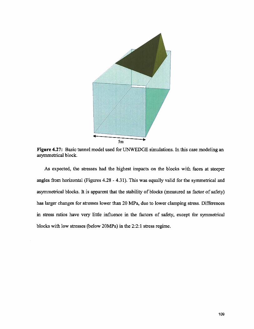
5m

Figure 4.27: Basic tunnel model used for UNWEDGE simulations. In this case modeling anasymmetrical block.

As expected, the stresses had the highest impacts on the blocks with faces at steeper

angles from horizontal (Figures 4.28 - 4.31). This was equally valid for the symmetrical and

asymmetrical blocks. It is apparent that the stability of blocks (measured as factor of safety)

has larger changes for stresses lower than 20 MPa, due to lower clamping stress. Differences

in stress ratios have very little influence in the factors of safety, except for symmetrical

blocks with low stresses (below 2OMPa) in the 2:2:1 stress regime.

109

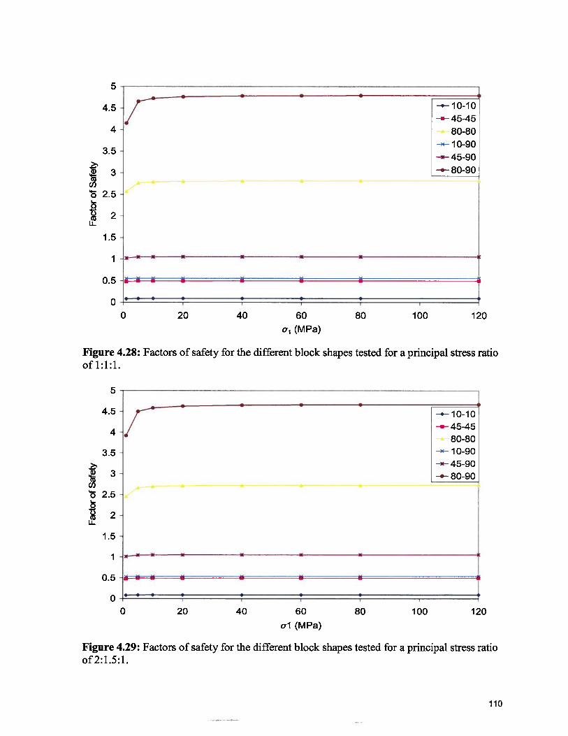
5

1010.7 —45-45

4 80-80—n-- 10-90

3.5-*-45-90

-.—80-90

Cl)

2.5

0CuLI

1.5

I K•— *

0.54I

i-. .•3- I I I

o 20 40 60 80 100 120o (MPa)

Figure 4.28: Factors of safety for the different block shapes tested for a principal stress ratioof 1:1:1.

5

4.5 : 10-10

4 /3.5 --10-90

—*--45903 —80-90

2.5

0 20 40 60 80 100 120

al (MPa)

Figure 4.29: Factors of safety for the different block shapes tested for a principal stress ratioof 2:1.5:1.

110

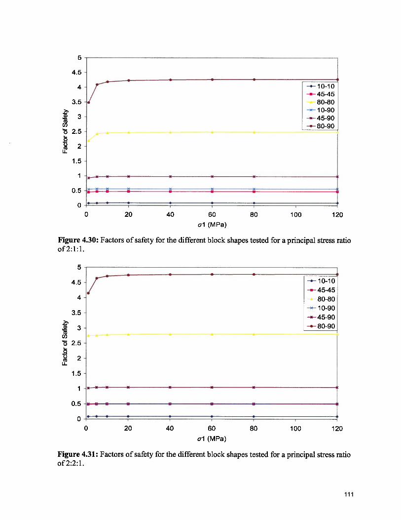
oj

_+

)—

.—

.F

acto

rof

Saf

ety

Fac

tor

ofS

afet

yo

-o

-

01

-1

1’.)

1c,

i101

Dol

.-

c)01

.t.

(3101

•0

II

II

I0

—I

II

II

I

— o0

I-I

Cl)

Cl)

o0

00

Cl)

Cl)

CD CD-L

o-U

0

Cl)

Cl)

CDCD

Cl)

Cl)

CD0

Cl)

CDCD

I

_______

z•

__

__

__

0

__

__

__

__

__

__

__

__

__

__

_

0

oc31000lo

100100o101

(DII

II

II

ICD

ItI

II

Iii

(I)

J(C)

(0(0

OD4

-Cl

)CD

CDCO

-I

Cl)

-0

00

001

0Cd

)

__

__

__

__

__

0000010[

F)

0-

0

o0

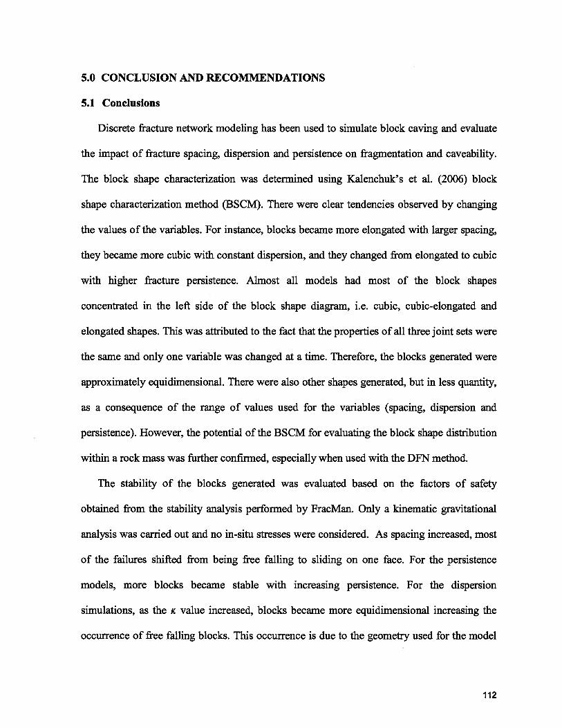
5.0 CONCLUSION AND RECOMMENDATIONS

5.1 Conclusions

Discrete fracture network modeling has been used to simulate block caving and evaluate

the impact of fracture spacing, dispersion and persistence on fragmentation and caveability.

The block shape characterization was determined using Kalenchuk’s et al. (2006) block

shape characterization method (BSCM). There were clear tendencies observed by changing

the values of the variables. For instance, blocks became more elongated with larger spacing,

they became more cubic with constant dispersion, and they changed from elongated to cubic

with higher fracture persistence. Almost all models had most of the block shapes

concentrated in the left side of the block shape diagram, i.e. cubic, cubic-elongated and

elongated shapes. This was attributed to the fact that the properties of all three joint sets were

the same and only one variable was changed at a time. Therefore, the blocks generated were

approximately equidimensional. There were also other shapes generated, but in less quantity,

as a consequence of the range of values used for the variables (spacing, dispersion and

persistence). However, the potential of the BSCM for evaluating the block shape distribution

within a rock mass was further confirmed, especially when used with the DFN method.

The stability of the blocks generated was evaluated based on the factors of safety

obtained from the stability analysis performed by FracMan. Only a kinematic gravitational

analysis was carried out and no in-situ stresses were considered. As spacing increased, most

of the failures shifted from being free falling to sliding on one face. For the persistence

models, more blocks became stable with increasing persistence. For the dispersion

simulations, as the K value increased, blocks became more equidimensional increasing the

occurrence of free falling blocks. This occurrence is due to the geometry used for the model

112

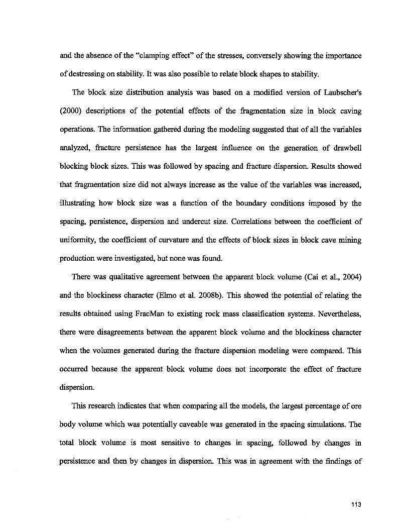
and the absence of the “clamping effect” of the stresses, conversely showing the importance

of destressing on stability. It was also possible to relate block shapes to stability.

The block size distribution analysis was based on a modified version of Laubscher’s

(2000) descriptions of the potential effects of the fragmentation size in block caving

operations. The information gathered during the modeling suggested that of all the variables

analyzed, fracture persistence has the largest influence on the generation of drawbell

blocking block sizes. This was followed by spacing and fracture dispersion. Results showed

that fragmentation size did not always increase as the value of the variables was increased,

illustrating how block size was a function of the boundary conditions imposed by the

spacing, persistence, dispersion and undercut size. Correlations between the coefficient of

uniformity, the coefficient of curvature and the effects of block sizes in block cave mining

production were investigated, but none was found.

There was qualitative agreement between the apparent block volume (Cai et al., 2004)

and the blockiness character (Elmo et al. 2008b). This showed the potential of relating the

results obtained using FracMan to existing rock mass classification systems. Nevertheless,

there were disagreements between the apparent block volume and the blockiness character

when the volumes generated during the fracture dispersion modeling were compared. This

occurred because the apparent block volume does not incorporate the effect of fracture

dispersion.

This research indicates that when comparing all the models, the largest percentage of ore

body volume which was potentially caveable was generated in the spacing simulations. The

total block volume is most sensitive to changes in spacing, followed by changes in

persistence and then by changes in dispersion. This was in agreement with the findings of

113

Chan and Goodman (1987), and Hoerger and Young (1990). They observed that in a three

joint set network, the total volume generated was sensitive mainly to fracture spacing. There

were limitations observed between the two dimensional (total block area on undercut) and

three dimensional (total block volume) evaluation of potential caveability. The measurements

of the block area on the undercut proved to be unreliable as means of assessing the blocks

that were potentially caveable. It is recommended that the block volume is used for this

purpose.

A brief analysis was carried out using UNWEDGE to determine the effect of stress on the

stability of blocks. Increases in stress had the largest impact on the factor of safety for blocks

with steep vertices. This was expected, since the stress acts more perpendicular to the block

face.

Based on the work carried out in this thesis, the potential of DFN for primary

fragmentation evaluation and determination was confirmed. DFN modeling shows great

potential for caveability assessment, and the study of the factors influencing the caving

process.

5.2 Recommendations for Further Work

Some of the recommendations for further study include extending the modeling

performed in this thesis to inhomogeneous ore bodies. As observed during the block shape

analysis, it is necessary to evaluate models with different values of spacing, dispersion and

persistence in all three dimensions. To further extend this research is also necessary to

incorporate rock mass properties into the DFN models including rock strength and joint

properties, as well as stress fields.

114

It is also suggested that the apparent block volume is modified to incorporate the effects

of dispersion.

No reliable data was found in order to verify the results. Case studies with reliable data

need to be modeled and compared to the synthetic simulations generated. This research

showed the potential of the DFN for evaluating fragmentation. It is important to verify these

findings by relating information gathered during the exploration and development faces of a

block cave mine with the fragmentation and hang up data from the production face.

It is also important to investigate the impact of secondary fragmentation on the blocks

formed during the primary fragmentation process.

115

REFERENCES

Barton, N., Lien, R., Lunde, J. 1974. Engineering classification of rock masses for the designof tunnel support. In: Rock Mechanics, Vol. 6, No. 4, 189-236.

Baecher, G.B., Lanney, N.A., Einstein, H.H. 1978. Statistical description of rock propertiesand sampling. In: Proceedings of the 18t1 Symposium on Rock Mechanics, Keystone,Colorado, 1-8.

Baecher, G.B. 1983. Statistical analysis of rock mass fracturing. In: Mathematical Geology,Vol. 15, No. 2, 329-348.

Beck, D., Arndt, S., Thin, I., Stone’ C., Butcher, R. 2006a. A conceptual sequence for a blockcave in an extreme stress and deformation environment. In: Third International Seminar onDeep and High Stress Mining 2006, Quebec City, Canada, 1-16.

Beck, D., F. Reusch, F., Arndt, S., Thin, I., Stone, C., Heap, M., Tyler, D. 2006b. Numericalmodeling of seismogenic development during cave initiation, propagation and breakthrough.In: Third International Seminar on Deep and High Stress Mining 2006, Quebec City,Canada, 1-15.

Bieniawski, Z. T. 1976. Rock mass classification in rock engineering. In: Exploration forRock Engineering, Ed. Z.T. Bieniawski, Balkema, Cape Town, 97-106.

Brown, E.T. 2003. Block caving geomechanics, The International Caving Study Stage I1997-2000, Julius Kruttschnitt Mineral Research Centre, Brisbane, Australia.

Brown, E.T. 2005. De Beers short course on block caving mechanics, SMJJJKMRCUniversity of Queensland and Golder Associates.

Butcher, R.J., Thin, I.G.T. 2007. The inputs and choices for predicting fragmentation inblock cave projects. In: 1st International Symposium on Block and Sub-level Caving CaveMining, Cape Town, South Africa, 3 5-50.

Cai, M., Kaiser, P.K., Uno, H., Tasaka, Y., Minami, M. 2004. Estimation of rock massdeformation modulus and strength of jointed hard rock masses using the GSI system. In:International Journal ofRockMechanics and Mining Sciences, Vol. 41, 3-19.

Capes, G., Milne, D. 2008. A compilation of dilution graph data for open stope hangingwalldesign. In: 1st Southern Hemisphere International Rock Mechanics Symposium, Vol. 1, 149-162.

Chan, L-Y., Goodman, R.E. 1987. Predicting the number and dimensions of the blocks of anexcavation using block theory and joint statistics. In: Proceedings of the 28th US Symposiumon Rock Mechanics, Tucson, Arizona, 81-87.

116

Coduto, D.P. 1999. Geotechnical engineering: principles and practices. Prentice Hall, NewJersey, USA.

Cundall, P. A., Hart, R.D. 1993. Numerical modeling of discontinua, In: ComprehensiveRock Engineering, Vol. 2, 231-243. J. A. Hudson, Ed. Oxford: Pergamon Press, 1993.

Cundall, P.A., Pierce, M.E., Mas Ivars, D. 2008. Quantifying the size effect of rock massstrength, In: 1S1 Southern Hemisphere International Rock Mechanics Symposium, Vol. 2, 3-16.

Deere, D.U. 1963. Technical description of rock cores for engineering purposes. In: RockMechanics and RockEngineering, Vol. 1, No. 1, 17-22.

Dershowitz, W.S., Einstein, H.H. 1988. Characterizing rock joint geometry with joint systemmodels. In: Rock Mechanics and Rock Engineering, Vol. 21, 21-51.

Dershowitz, W.S., 1992. The role of the stripa phase 3 project in the development of practicaldiscrete fracture modeling technology. In: Proceedings of the 4th International NEA/SKBSymposium, Stockholm, 237-258

Dershowitz, W.S., Herda, H. 1992. Interpretation of fracture spacing and intensity. In:Proceedings ofthe 33’’ US Rock Mechanics Symposium, Publ. 33, 75 7-766.

Dershowitz, W.S., LaPointe, P., Eiben, T., Wei, L. 1998a. Integration of discrete featurenetwork methods with conventional approaches. In: Society of Petroleum Engineers, Paper49069.

Dershowitz, W.S., Lee, G., Geier, J. and LaPointe, P.R. 1998b. FracMan: Interactive discretefeature data analysis. Geometric modelling and exploration simulation. User Documentation.Golder Associates Inc. Seattle - Washington.

Duplancic, P., Brady, B.H. 1999, Characterization of caving mechanisms by analysis ofseismicity and rock stress. In: Proceedings of the 9th International Congress on RockMechanics. Vol. 2, 1049-1053.

Duplancic, P. 2001. Characterisation of caving mechanisms through analysis of stress andseismicity, PhD thesis, Department of Civil and Resource Engineering, University ofWestern Australia.

Eadie, B.A. 2002. Modelling primary and secondary fragmentation for block caving. PhDThesis, University of Queensland, Brisbane.

Elmo, D., Vyazmensky, A., Stead, D., Rance, J. R. 2007a. A hybrid FEMJDEM approach tomodel the interaction between open pit and underground block caving mining. In:Proceedings of the 1st Canadian-US Rock Mechanics Symposium, Vancouver, Canada, Vol2, 1287-1294.

117

Elmo, D., Yan, M., Stead, D., Rogers, S.F. 2007b. The importance of intact rock bridges inthe stability of high rock slopes: towards a quantitative investigation using and integratednumerical modeling — discrete fracture network approach. In: Proceedings of theInternational Symposium on Rock Slope Stability in Open Pit Mining and Civil Engineering.Perth, Australia.

Elmo D., Vyazmensky, A., Stead, D., Rance. J. 2008a. Numerical analysis of pit walldeformation induced by block caving mining. In: Proceedings of the 5th Conference andExhibition on Mass Mining, Lulea, Sweden, June 2008, 1073-1082.

Elmo D., Stead D., Rogers S. 2008b. A quantitative analysis of a fractured rock mass using adiscrete fracture network approach: characterisation of natural fragmentation andimplications for current rock mass classification systems. In: Proceedings of the 5thConference and Exhibition on Mass Mining, Lulea, Sweden, June 2008, 1023-1032.

Einstein, H.H., Baecher, G.B. 1983. Probabilistic and statistical methods in engineeringgeology, specific methods and examples, part I: exploration. In: Rock Mechanics and RockEngineering, Vol. 16, 39-72.

Esci, L., Dutko, M. 2003. Large scale fracturing and rock flow using discrete elementmethod, 2D application for block caving. In: Numerical Methods in Continuum Mechanics,Zilina, Slovak Republic.

Esterhuizen, G.S. 1994. A program to predict block cave fragmentation. Technical Referenceand User’s Guide, Version 2.1.

Fisher, R.A. 1953. Dispersion on a sphere. In: Proceedings of the Royal Society ofLondon,A217, 295-305.

Flores, G., Karzulovic, A. 2003. Geotechnical guidelines for a transition from open pit tounderground mining, geotechnical guidelines. In: International Caving Study I] Task 4.

Geo&Soft. 1999. Geo&Soft International, ROCK3D — identification, geometricreconstruction and stabilization of complex rock blocks, User’s Guide and Windows BasedCode.

Gilbride, L.J., Free, K.S., Kehrman, R. 2005. Modeling block cave subsidence at MolycorpInc., Questa Mine. In: Proceedings of the 40th US. Symposium on Rock Mechanics,ARMA/USRMS 05-88 1, Anchorage, Alaska.

Golder Associates, 2007. FracMan Version 6.54. FracMan Technology Group.

Goodman, R.E., Shi, G. H. 1985. Block theory and its application to rock engineering.Prentice-Hall, Englewood Cliffs, New Jersey.

118

Goodman, R.E. 1995. Block theory and its application. In: Geotechnique, Vol. 45, No. 3,383-423.

Grenon, M., Hadjigeorgiou, J., 2003. Evaluating discontinuity network characterization toolsthrough mining case studies. In: Soil Rock America 2003, Vol. 1, 137-142.

Hadjigeorgiou, J., Lessard, J.F., Flament, F. 1995. Characterizing in situ block sizedistribution using stereological model. In: Canadian Tunnelling Journal, 201-211.

Hadjigeorgiou, J., Esmaieli, K., Grenon, M. 2008. Stability analysis of vertical excavations inhard rock by integrating a fracture system into a PFC model. In: Tunnelling andUnderground Space Technology, article in press.

Hoek, E. 1994. Strength of rock and rock masses. In: ISRM News Journal, Vol. 2, No. 2, 4-16.

Hoek, E., Carranza-Torres, C.T., Corcum, B. 2002. Hoek-Brown failure criterion 2002edition. In: Proceedings of the North American Rock Mechanics Society (NARMS-TAC2002), Bawden, Curran and Telsenicki, editors. Mining Innovation and Technology, Toronto,267-273.

Hoerger, S.F., Young, D.S. 1990. Probabilistic prediction of key block occurrences. In: RockMechanics Contributions and Challenges. Hustrulid and Johnson, editors. Rotterdam:Balkema. 229-236.

Itasca (2008) PFC and PFC3D version 4.0 Itasca Consulting Group, Inc., Minneapolis.

Itasca (2004a) UDEC version 4.0 Itasca Consulting Group, Inc., Minneapolis.

Itasca (2004b) 3DEC version 4.0 Itasca Consulting Group, Inc., Minneapolis.

Itasca (2004c) FLAC3D version 3.0 Itasca Consulting Group, Inc. Minneapolis.

Itasca (2004d) Rebop version 2.1 Itasca Consulting Group, Inc. Minneapolis.

Itasca (2005) FLAC version 5.0 Itasca Consulting Group, Inc., Minneapolis.

Jimenez-Rodriguez, R., Sitar, N. 2006. Inference of discontinuity trace length distributionsusing statistical graphical models. In: International Journal of Rock Mechanics and MiningSciences, Vol. 43, 877-893.

Jing, L. 2003. A review of techniques, advances and outstanding issues in numericalmodelling for rock mechanics and rock engineering. In: International Journal of RockMechanics and Mining Sciences, Vol. 40, 283-3 53.

119

Jing, L., Stephansson, 0. 2007. Fundamentals of discrete element methods for rockengineering, Theory and Applications, Elsevier Science.

Jakubowski, J. 1995. Prediction of the load of tunnel support in rock mass of blocky structureby statistical methods, PhD dissertation, University of Mining and Metallurgy, Krakow,Poland.

Kalenchuk, K.S., Diedrichs, M.S., McKinnon, 5. 2006. Characterizing block geometry injointed rock masses. In: International Journal ofRock Mechanics and Mining Sciences, Vol.43, 1212-1225.

Kalenchuk, K.S., McKinnon, S., Diedrichs, M.S. 2007a. Block Geometry and RockmassCharacterization for Prediction of Dilution Potential into Sub-level Cave Mine Voids. In:International Journal ofRock Mechanics and Mining Sciences, in press.

Kalenchuk, K.S., McKimion, S., Diedrichs, M.S. 2007b. Dilution source prediction andcharacterization for blocky rock masses in steep walls or cave boundaries for bulk mining.In: 1st International Symposium on Block and Sub-level Caving Cave Mining, Cape Town,South Africa, 83-94.

Karzulovic, A., Cavieres, P., Pardo, C. 1999. Subsidencia por efecto del caving en mina ElTeniente. In: Internal Report Area de Ingenieria de Rocas, Codelco Chile, Division ElTeniente, Estudio DT-8G-99-0G3.

Kendorski, F.S., Cummings, R.A., Bieniawski, Z. T. 1982. Caving mine rock massclassification and support estimation. In: Engineers International Inc. Contract Report no.J0100103 to US Bureau ofMines.

Kim, B.H., Cai, M., Kaiser, P.K., Yang, H.S. 2007. Estimation of block sizes for rock masseswith non-persistent joints. In: Rock Mechanics and Rock Engineering, Vol. 40, No.2, 169-192.

Laubscher, D. 1990. A geomechanics classification system for the rating of rock mass inmine design. In: Journal of the South African Institute of Mining and Metallurgy, Vol. 90,No.10, 257-273.

Laubscher, D. 2000. A practical manual on block caving. Prepared for the InternationalCaving Study. JKMRC and Itasca Consulting Group, Inc.

Layton, G.W., Kingdon, R.D., Herbert, A.W. 1992. The application of a three-dimensionalfracture network model to a hot-dry-rock reservoir. In: Rock Mechanics, Tillerson, J.R. andWarwersik, W.R. editors, Balkema, Rotterdam, 561-570.

Li, H., Brummer, R. 2005. Analysis of pit wall failure mechanism and assessment of long-term stability of pit walls at Palabora Mine. In: Itasca Consulting Canada Ltd., TechnicalReport.

120

Maerz, N.H., Germain, P. 1995. Block size determination around underground openingsusing simulations based on scanline mapping. In: Proceedings of the Conference onFractured and Jointed Rock Masses, Lake Tahoe, 27-33.

Martin, C.D., Kaiser, P.K., Christiansson, R. 2003. Stress, instability and design ofunderground excavations. In: International Journal ofRock Mechanics and Mining Sciences,Vol. 40, No. 7-8, 1027-1047.

Mas Ivars, D., Pierce, M., DeGagne, D., Darcel, C. 2008. Anisotropy and scale dependencyin jointed rock mass strength — a synthetic rock mass study. In: Proceedings of the FirstInternational FLAC/DEM Symposium on Numerical Modeling, Hart et al. editors,Mineapolis, August 2008, Tn press.

Mathews, K.E., Hoek, E., Wyllie, D.C., Stewart, S.D.V. 1980. Prediction of stableexcavation spans for mining at depths below 1,000 metres in hard rock. In: Golder AssociatesReport to Canada Centre for Mining and Energy Technology (CANMET), Department ofEnergy and Resources, Ottawa, Canada.

Mauldon, M., Goodman, R. E. 1990. Rotational kinematics and equilibrium of blocks in arock mass. In: International Journal ofRock Mechanics and Mining Sciences, Vol. 27, No. 4,291-301.

Mauldon, M. 1995. Key block probabilities and size distributions: a first model forimpersistent 2-D fractures. In: International Journal of Rock Mechanics and MiningSciences, Vol. 32, No. 6, 575-583.

Mauldon, M, Goodman, R.E. 1996. Vector analysis of key block rotations. In: Journal ofGeotechnical Engineering, Vol. 122, No. 12, 976-987.

Mauldon, M. 1998. Estimating mean fracture trace length and density from observations inconvex windows. In: RockMechanics andRock Engineering, Vol.31, Iss.4, 201-216

Mawdesley, C., Trueman, R. and Whiten, W. 2001. Extending the Mathews stability graphfor open-stope design. In: Transactions of the Institution ofMining and Metallurgy, SectionA: Mining Technology. Vol. 110, Sect. A, 27-3 9.

Mawdesley, C. 2002. Predicting cave initiation and propagation in block caving mines.PhD Thesis, University of Queensland, Brisbane.

Mine Modeling. 2006. Map3D ver. 53, Mine Modeling Pty, Ltd, Australia.

Palmstrom, A. 1974. Characterization of jointing density and the quality of rock masses. In:Internal Report, A.B. Berdal, Norway.

121

Palmstrom, A. 1982. The volumetric joint count — a useful and simple measure of the degreeof rock mass jointing. In: IAEG Congress, New Delhi, 221-228.

Palmstrom, A. 1996. Characterizing rock masses by the RMi for use in practical rockengineering, part 1: the development of the rock mass index (RMi). In: Tunneling andUnderground Space Technology, Vol. 11, No. 2, 175-188.

Palmstrom, A. 2005. Measurements of and correlations between block size and rock qualitydesignation (RQD), In: Tunnelling and Underground Space Technology, Vol. 20, 362-377.

Palmstrom, A., Broch, E. 2006. Use and misuse of rock mass classification systems withparticular reference to the Q-system. In: Tunnelling and Underground Space Technology,Vol. 21, 575-593.

Pantechnica. 2000. Pantechnica Corporation, KBTunnel version 2.0 users manual, MN, EdenPrairie.

Pierce, M., Cundall, P., Potyondy, D., Mas Ivars, D. 2007. A synthetic rock mass model forjointed rock. In: Proceedings of the 1st Canadian-US Rock Mechanics Symposium,Vancouver; Canada, Vol 1, 341-349.

Pine, R.J., Coggan, J.S., Flynn, Z.N., Elmo, D. 2006. The development of a new numericalmodeling approach for naturally fractured rock masses. In: Rock Mechanics and RockEngineering, Vol. 39, No. 5, 395-419.

Priest, S.D. 1993. Discontinuity analysis for rock engineering. Chapman & Hall, London.

Priest, S.D., Samaniego, J.A. 1998. The statistical analysis of rigid block stability in jointedrock masses. In: Proceedings of the Ffih Australia-New Zealand Conference onGeomechanics, The Institutions of Engineers Australia, Sydney, 398-403.

Rance, J. M., van As, A., Owen, D. R. J., Pine, R. J. 2007. Computational modeling ofmultiple fragmentation in rock masses with application to block caving. In: Proceedings ofthe 1St Canadian-US Rock Mechanics Symposium, Vancouver; Canada, Vol 1, 477-484.

Read, J.R.L., Ogden, A.N. 2006. Developing new approaches to rock slope stability analyses.In: International Symposium on Stability of Rock Slopes in Open Pit Mining and CivilEngineering, 3-9.

Reyes-Montes, J.M., Pettitt, W. S., Young, R.P. 2007. Validation of a synthetic rock massmodel using excavation induced microseismicity. In: Proceedings of the 1t Canadian-USRock Mechanics Symposium, Vancouver; Canada, Vol 1, 365-369.

Rockfield. 2006. ELFEN, Rockfield Software Ltd. Swansea, UK.

Rocscience 2004. Phase2version 5.0, Rocscience Inc., Toronto, Canada.

122

Rocscience 2006. Swedge version 5.0, Rocscience Inc., Toronto, Canada.

Rocscience 2007. Unwedge version 3.0, Rocscience Inc., Toronto, Canada.

Rogers, S.F., Moffit, K.M., Kennard, D.K. 2006. Probabilistic slope and tunnel blockstability analysis using realistic fracture network models. In: The 4l’ US. Symposium onRock Mechanics (USRMS), ARMAIUSRMS 06-1052

Rogers, S.F., Kennard, D.K., Dershowitz, W.S., van As, A. 2007. Characterising the in situfragmentation of a fractured rock mass using a discrete fracture approach. In: Proceedings ofthe i Canadian-US RockMechanics Symposium, Vancouver, Canada, Vol 1, 137-143.

Rouleau, A., Gale, J.E. 1987. Stochastic discrete fracture simulation of groundwater flowinto underground excavation in granite. In: International Journal of Rock Mechanics andMining Sciences Abstracts, Vol. 24, No. 2, 99-112.

Sainsbury, B., Pierce, M., Mas Ivars, D. 2008. Simulation of rock mass strength anisotropyand scale effects using Ubiquitous Joint Rock Mass (UJRM) model. In: Proceedings of theFirst International FLAC/DEM Symposium on Numerical Modeling, Hart et al. editors,Mineapolis, August 2008, lii press.

Simulia. 2007. Abaqus, Inc. version 6.7, Simulia Dassault Systemes.

Singh, U.K., Stephanson, O.J., Herdocia, A. 1993. Simulation of progressive failure inhanging wall and foot wall for mining with sublevel caving. In: Transactions of theInstitution ofMining and Metallurgy, Section A: Mining Technology. Vol. 102, Sect. A, 188-194.

Split-Engineering, 2008. Split-Desktop version 2.0. Split Engineering LLC.

Staub, I., Fredriksson, A., Outers, N. 2002. Strategy for a rock mechanics site descriptivemodel, development and testing of the theoretical approach. Svensk KarnbranslehanteringAB, Rapport R-02-02, May 2002.

Starzec, P., Tsang, C.-F. 2002. Use of fracture-intersection density for predicting the volumeof unstable blocks in underground openings. lii: International Journal of Rock Mechanicsand Mining Sciences, Vol. 39, 807-813.

Stone, C.A. 1994. A matrix approach to probabilistic key block analysis, PhD dissertation,Michigan Technological University.

Sun Microsystems, 2008. Java Standard Edition 6, Sun Microsystems, Inc.

Terzaghi, R.D. 1965. Sources of error in joint surveys. In: Geotechnique, Vol. 15, No. 3,287-304.

123

Tonon, F. 1998. Generalization of Mauldon’s and Goodman’s vector analysis of key blockrotations. In: Journal of Geotechnical and Geoenvironmental Engineering, Vol. 124, No. 10,913-922.

Villaescusa, E. 1991. A three dimensional model of rock jointing. PhD thesis, University ofQueensland, Brisbane.

Vyazmensky, A., Elmo, D., Stead, D., Rance, J.R. 2007. Combined finite-discrete elementmodelling of surface subsidence associated with block caving mining. In: Proceedings of thejst Canadian-US RockMechanics Symposium, Vancouver, Canada, Vol 1, 467-475.

Vyazmensky A., Elmo D., Stead D., Rance J. 2008. Numerical analysis of the influence ofgeological structures on development of surface subsidence associated with block cavingmining. In: Proceedings of the 5th Conference and Exhibition on Mass Mining, Lulea,Sweden, June 2008, 857-866

Wang, L.G., Yamashita, S., Sugimoto, F., Pan, C., Tan, G. 2003. A methodology forpredicting the in situ size and shape distribution of rock blocks. In: Rock Mechanics andRock Engineering, Vol. 36, No. 2, 12 1-142.

Warburton, P.M. 1981. Vector stability analysis of an arbitrary polyhedral rock block withany number of free faces. In: International Journal ofRock Mechanics and Mining Sciences,Vol. 18, No. 5, 415-427.

Watababe, K., Takahashi, H. 1995. Parametric study of the energy extraction from hot dryrock based on fractal fracture network model. In: Geothermics, Vol. 24, No. 2, 223-236.

Windsor, C.R., Thompson, A.G. 1991. Reinforcement design for jointed rock masses, In: The33rd US Symposium on RockMechanics, 520-521.

Wyllie, D.C., Mah, C.W. 2004. Rock slope engineering: civil and mining 4th edition. SponPress, Francis and Taylor Group, New York, USA.

Zhang, L., Einstein, H.H. 1998. Estimating mean trace length of rock discontinuities. In:Rock Mechanics and Rock Engineering, Vol. 31, 217-235.

Zhang, L., Einstein, H.H. 2000. Estimating the intensity of rock discontinuities. In:International Journal ofRock Mechanics and Mining Sciences, Vol. 37, 8 19-837.

124

APPENDIX AJava Application Code

125

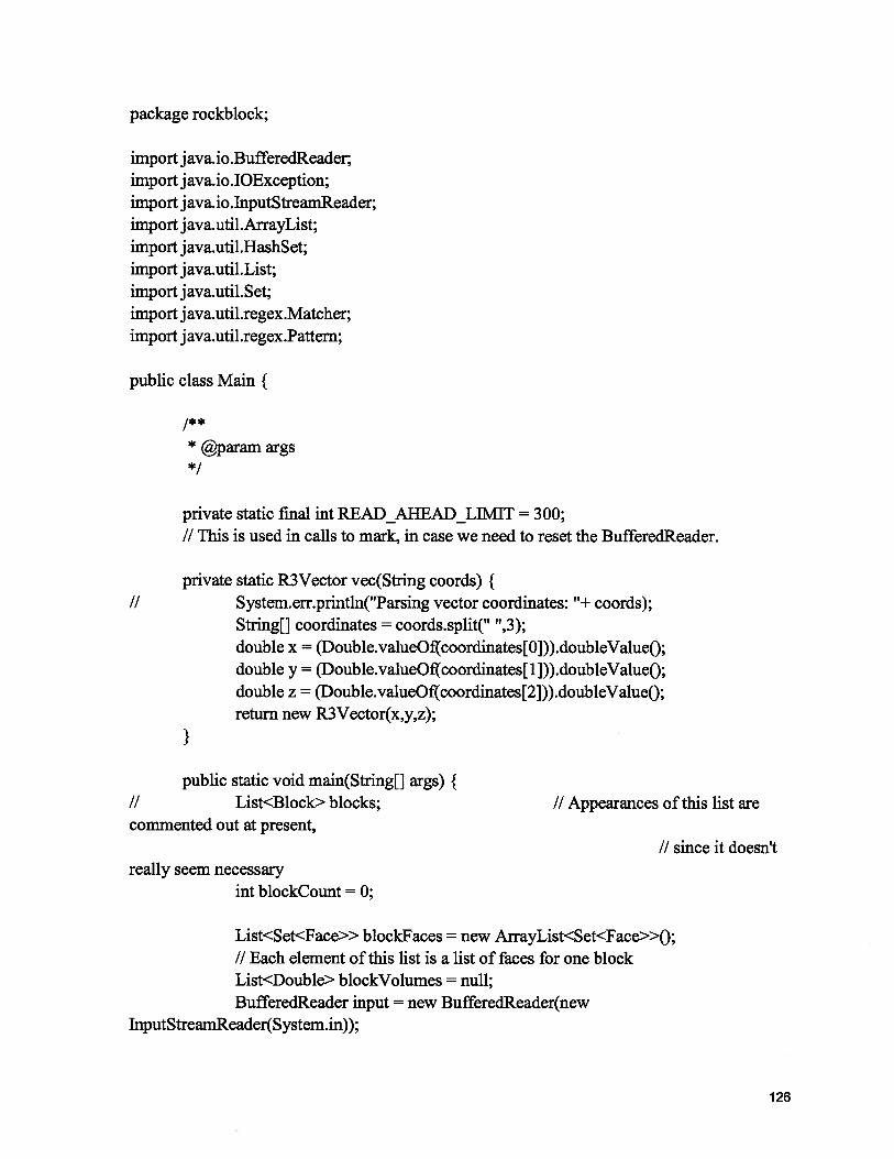
package rockblock;

import j ava.io.BufferedReader;import j ava.io.IOException;import java.io.TnputStreamReader;import java.util.ArrayList;import java.util.HashSet;import java.util.List;import java.util.Set;import java.util.regex.Matcher;import j ava.util.regex.Pattern;

public class Main {

1* *

* @param args*1

private static final mt READ_AHEAD_LIMIT = 300;II This is used in calls to mark, in case we need to reset the BufferedReader.

private static R3Vector vec(String coords) {II System.err.println(”Parsing vector coordinates: “+ coords);

String[] coordinates = coords.split(” “,3);double x = (Double.valueOf(coordinates[0])).doubleValueO;double y = (Double.valueOf(coordinates[ 1 ])).doubleValueO;double z = (Double.valueOf(coordinates[2fl).doubleValueO;return new R3Vector(x,y,z);

}

public static void main(String[] args) {II List<Block> blocks; II Appearances of this list arecommented out at present,

II since it doesn’treally seem necessary

mt blockCount =0;

List<Set<Face>> blockFaces = new ArrayList<Set<Face>>;II Each element of this list is a list of faces for one blockList<Double> blockVolumes = null;BufferedReader input = new BufferedReader(new

InputStreamReader(System.in));

126

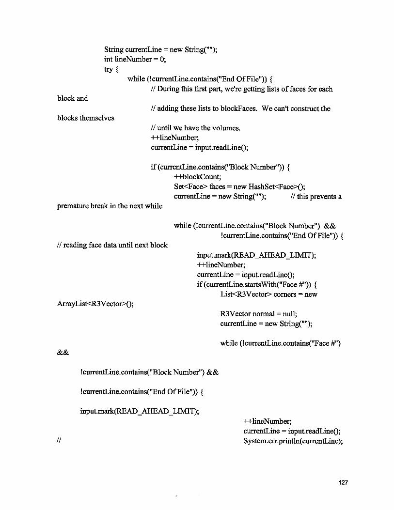
String currentLine = new String(”);mt lineNumber =0;try{

while (!currentLine.contains(”End Of File”)) {II During this first part, we’re getting lists of faces for each

block andII adding these lists to blockFaces. We can’t construct the

blocks themselvesII until we have the volumes.++lineNumber;currentLine = input.readLineO;

if (currentLine.contains(”Block Number”)) {++blockCount;Set<Face> faces = new HashSet<Face>O;currentLine = new String(”); I/this prevents a

premature break in the next while

while (!currentLine.contains(”Block Number”) &&currentLine.contains(”End Of File”)) {

II reading face data until next blockinput.mark(READ_AIIEAD_LIMIT);++lineNumber;currentLine = input.readLineO;if (currentLine.startsWith(”Face #“)) {

List<R3Vector> corners = newArrayList<R3Vector>O;

R3Vector normal = null;currentLine = new String(”);

while (!currentLine.contains(”Face #“)

&&

currentLine.contains(”Block Number”) &&

currentLine.contains(”End Of File”)) {

input.mark(READ_AHEAD_LIMIT);++lineNumber;currentLine = input.readLineO;System.err.println(currentLine);

127

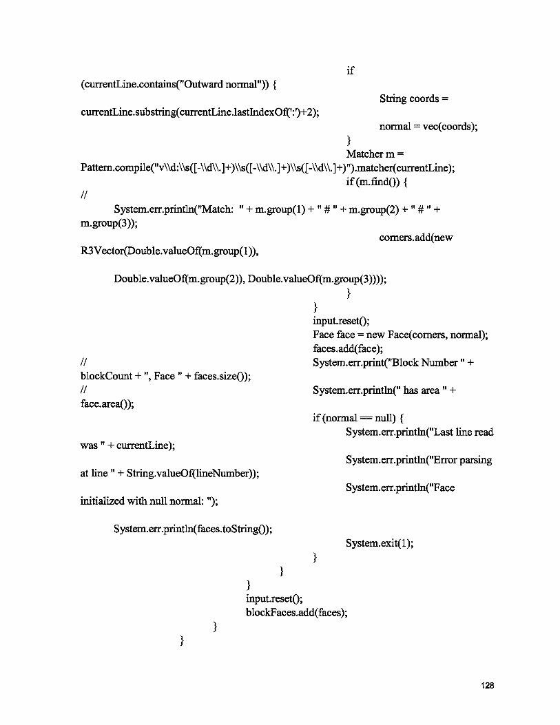
if

}}

}}

input.resetO;Face face = new Face(comers, normal);faces.add(face);System.err.print(”Block Number “ +

System.err.println(” has area” +

if (normal == null) {System.err.println(”Last line read

System.err.println(”Error parsing

System.err.println(”Face

}

input.resetO;blockFaces.add(faces);

System.exit( 1);

(currentLine.contains(”Outward normal”)) {String coords =

currentLine.substring(currentLine.lastlndexOf(’:‘)+2);normal = vec(coords);

}Matcher m =

Pattem.compile(”v\\d:\\s([-\\d\\.]+)\\s([-\\d\\.]+)\\s([-\\d\\.]+)”).matcher(currentLine);if(m.findQ) {

IISystem.err.println(”Match: “+ m.group(1) + “# “ + m.group(2) +“ # “+

m.group(3));corners.add(new

R3Vector(Double.valueOf(m.group(1)),

Double.valueOf(m.group(2)), Double.valueOf(m.group(3))));

}}

IIblockCount + “, Face “ + faces.sizeO);IIface.areaQ);

was “+ currentLine);

at line” + String.valueOf(lineNumber));

initialized with null normal: “);

System.err.println(faces.toStringO);

128

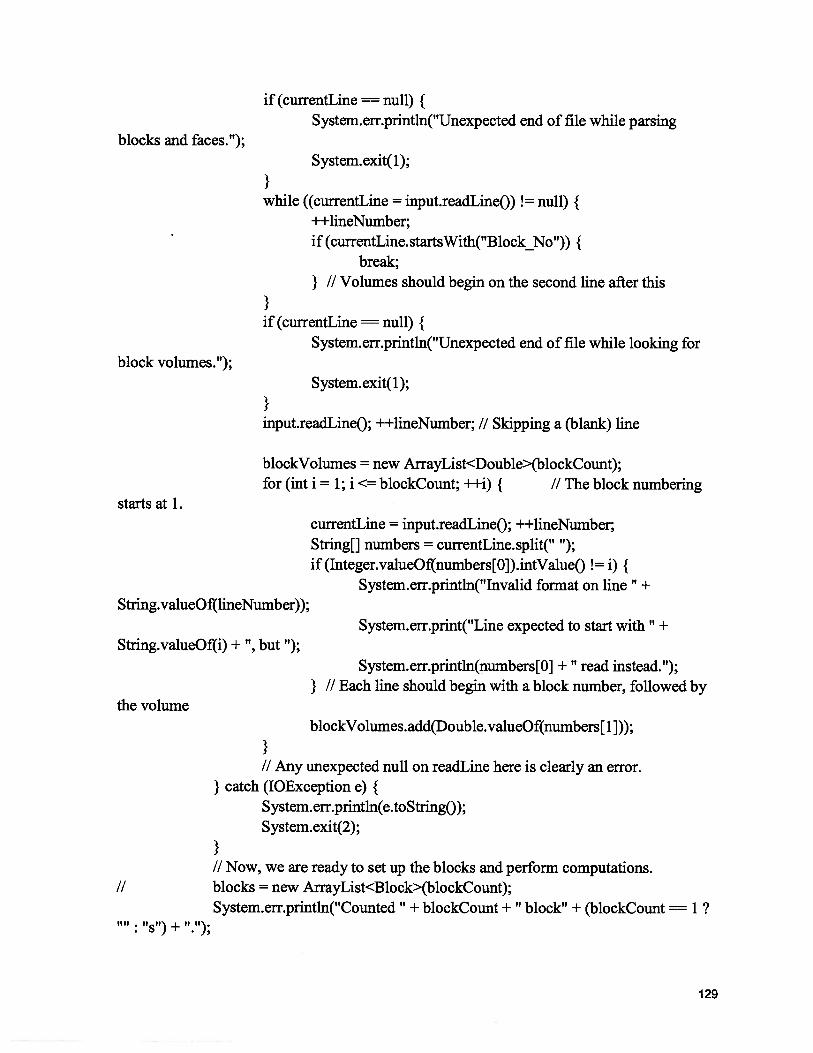
if (currentLine = null) {System.err.println(”Unexpected end of file while parsing

blocks and faces.”);System.exit( 1);

}while ((currentLine = input.readLineO) ! null) {

++lineNumber;if (currentLine. startsWith(”Block No”)) {

break;

} II Volumes should begin on the second line after this

}if (currentLine = null) {

System.err.println(”Unexpected end of file while looking forblock volumes.”);

System.exit(l);

}input.readLineO; ++lineNumber; // Skipping a (blank) line

blockVolumes = new ArrayList<Double>(blockCount);for (mt = 1; i <= blockCount; ++i) { // The block numbering

starts at 1.currentLine = input.readLineO; ++lineNumber;String[] numbers = currentLine.split(” “);if (Tnteger.valueOf(numbers[O]).intValueO != i) {

System.err.println(”Invalid format on line” +

String.valueOf(lineNumber));System.err.print(”Line expected to start with “ +

String.valueOf(i) + “, but “);

System.err.println(numbers[Oj + “read instead.”);

} // Each line should begin with a block number, followed bythe volume

blockVolumes.add(Double.valueOf(numbers[11));}II Any unexpected null on readLine here is clearly an error.

} catch (JOException e) {System.err.println(e.toStringO);System.exit(2);

}II Now, we are ready to set up the blocks and perform computations.blocks = new ArrayList<Block>(blockCount);System.err.println(”Counted” + blockCount + “block” + (blockCount = 1?

: ‘‘s’’) —I— ‘

‘‘);

129

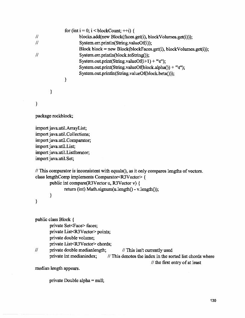
for (mt = 0; i <blockCount; ++i) {II blocks.add(new Block(faces.get(i), blockVolumes.get(i)));II System.err.println(String.valueOf(i));

Block block = new Block(blockFaces.get(i), blockVolumes.get(i));II System.err.println(block.toStringO);

System.out.print(String.valueOf(i+ 1) +

System.out.print(String.valueOf(block.alphaO) +

System.out.println(String.valueOf(block.betaO));

}

}

}

package rockblock;

import j ava.util.ArrayList;import j ava.util.Collections;import j ava.utiLComparator;import java.utiLList;import j ava.util.Listlterator;import java.util.Set;

II This comparator is inconsistent with equalsO, as it oniy compares lengths of vectors.class lengthComp implements Comparator<R3Vector> {

public mt compare(R3Vector u, R3Vector v) {return (int) Math.signum(u.length() - v.lengthO);

}}

public class Block {private Set<Face> faces;private List<R3Vector> points;private double volume;private List<R3Vector> chords;

II private double medianlength; II This isn’t currently usedprivate mt medianindex; II This denotes the index in the sorted list chords where

I/the first entry of at leastmedian length appears.

private Double alpha = null;

130

private Double beta = null;II These are used to cache the values of alpha and beta, so that if they are queried

moreI/than once on any particular Block, they need not be recomputed.II (Double objects are used instead of doubles because null is a convenient initial

value.)

public Block(Set<Face> faces, double volume) {this.volume = volume;this.faces = faces;points = new ArrayList<R3Vector)’;II We take care here not to add the same point twice. I was going to use Set

for this (withII HashSet implementing), but it’s handy to use a List in the next part.for (Face face : faces) {

for (R3Vector point: face.cornersO) {if (!points.contains(point)) points.add(point);

}}II Now we go on to set up our list of all chord lengths from one distinct point

to anotherII with a total ofp*(pl )/2 such lengths

mt p = points.sizeO;chords = new ArrayList<R3Vector>(p*(p 1)72);for (inti=O; i<p; ++i) {

for(intji+1;j<p;++j) {R3Vector chord = points.get(i).subQ,oints.get(j));System.err.print(”Chord “ + chord.toStringO + “ computed

from point” + i);System.err.println(” minus point “+j +

chords.add(chord);

}}Collections.sort(chords, new lengthCompO);mt n chords.sizeO;

System.err.println(”Found” + n +“ chords.”); II DIAGNOSTIC

if (n%2== 0) {medianindex = n12; II e.g. with 14 chords (indices 0-

13), index 7 is just above median

131

II medianlength = (chords.get(medianindex - l).lengthQ +

chords.get(medianindex).lengthO)/2;

} else {medianindex = (n-1)/2; II e.g. with 15 chords, index 7 is

at the medianII medianlength = chords.get(medianindex).lengthO;

}}

public double alpha() {if(alpha != null) {

return alpha.doubleValueO;}double surfaceArea =0;for (Face face: faces) {

surfaceArea += face.area();

}double meanLength =0;double n chords.sizeO;for (R3Vector v : chords) {

meanLength += v.length() / n;

}II System.err.println(”Total length: “+ meanLength*n + “with “ + chords.size()+ “ chords.”); II DIAGNOSTICII System.err.print(”Surface area: “+ surfaceArea + “\t” + “Mean length: “+

meanLength);// System.err.println(”\tVolume: “+ volume);DIAGNOSTIC

return (alpha = surfaceArea * meanLength) / (7.7 * volume);return and store value

}

public double betaO {if (beta != null) {

return beta.doubleValueO;}

II Here, we take only those chords of at least median length.List<R3Vector> longChords = chords. subList(medianindex, chords.sizeO);

II DIAGNOSTIC

132

II System.err.print(”Of” + chords.size() + “total chords, “+ longChords.size() +

of at least”);II System.err.println(” median length are used to compute beta.”);

II In the numerator, we take a sum of squares of dot products over all pairsII (a,b) of long enough chords s.t. a != b and only one of(a,b), (b,a) appears.double topSum = 0;I/In the denominator, there is a sum of aI’’2Ibl’2 over such pairs.double bottomSum =0;

II String numeratorDiagnostics =II String denominatorDiagnostics = “;

for (Listlterator<R3Vector> i = longChords.listlteratorO; i.hasNextO;) {R3Vector a i.nextO;

II System.err.println(”Long chord” + a.toString() +“ found.\tlts length is“+ a.length()); II DIAGNOSTIC

for (Listlterator<R3Vector> j = longChords.listlterator(i.nextlndexO);j.hasNextO;) {

R3Vector b j .nextO;double numeratorTerm = Math.pow(a.dot(b),2);double denominatorTemi = a.dot(a) * b.dot(b);

II numeratorDiagnostics += “Adding (“ + a + “ dot “ + b +“)‘2 =

“+ numeratorTerm + “to numerator.\n”;II denominatorDiagnostics += “Adding

“+ a + “I’2 “

+ b +

=“ + denominatorTerm +“to denominator.\n”;topSum += numeratorTerm;

//Math.pow(a.dot(b), 2);bottomSum += denominatorTerm; //a.dot(a) *

b.dot(b);

}}

II System.err.println(numeratorDiagnostics);II System.err.println(denominatorDiagnostics);

return beta = 10 * Math.pow((topSum / bottomSum),2); 7/ returnand store value

}

public String toString() {return “Volume: “+ volume + “\n” + “Faces: “+ faces.toString() + “\n” +

“Points: “ + points.toStringO;

}

133

}

package rockblock;import j ava.util.Iterator;import java.util.List;

public class Face {private List<R3Vector> corners;private R3Vector normal;

public Face(List<R3Vector> corners, R3Vector normal) {this.corners = corners;this.normal = normal;

}

public List<R3Vector> corners() {return this.corners;

}public R3Vector normal() {

return normal;

}

public double area() {II As an unfortunate hack, I’m currently going to return zero area in situationsII such as having no corners. I probably want to revisit this and maybe useII exceptions.if (corners.isEmptyO) return 0;R3Vector cumulative = R3Vector.origin;

II Here we want to add up successive cross products, starting with the firstpoint cross the

II second, etc. up to the last point cross the first.Iterator<R3Vector> i = corners.iteratorO;R3Vector firstPoint = i.nextQ;R3Vector currentPoint;R3Vector nextPoint = firstPoint;while (i.hasNextO) {

currentPoint = nextPoint;nextPoint = i.nextO;cumulative = cumulative.add(currentPoint.cross(nextPoint));

}cumulative = cumulative.add(nextPoint.cross(flrstPoint));

134

// Hopefully taking the absolute value will make sure we get an actual area.return Math.abs(normal.dot(cumulative))/2;II Note that, if there is only one point in the set of corners, the while loop will

never activate// and we will obtain zero == firstPoint.cross(firstPoint) in the current

implementation.

}public String toString() {

return “Normal” + normal.toStringO + “, Corners: “+ corners.toStringO;}

}

package rockblock;

public class R3Vector {private double x, y, z;fmal public static R3Vector origin = new R3Vector(O,O,O);

public R3Vector(double x, double y, double z) {this.x = x;this.y = y;tbis.z=z;

}

public double x() {return x;

}public double yO {

return y;

}public double z() {

return z;

}

public R3Vector scalarmult(double c) {return new R3Vector(c * this.x, c * this.y, c * this.z);

}public R3Vector add(R3Vector v) {

return new R3Vector(this.x + v.x, this.y + v.y, this.z + v.z);}public R3Vector sub(R3Vector v) {

135

return new R3Vector(this.x - v.x, this.y - v.y, this.z - v.z);

}public double dot(R3Vector v) {

return this.x * v.x + this.y * v.y + this.z * v.z;

}public R3Vector cross(R3Vector v) {

return new R3Vector(this.y * v.z - this.z * v.y,this.z * v.x - this.x * v.z,this.x * v.y - this.y * v.x);

}public double distance(R3Vector v) {

return java.lang.Math.sqrt( (this.x - v.x) * (this.x - v.x) +

(this.y - v.y) * (this.y -

v.y) +

(this.z - v.z) * (this.z -

v.z));

}public double length() {

return distance(origin);

}

public boolean equals(Object o) {if(!(o instanceofR3Vector)) return false;R3Vector v = (R3Vector) o;if (this.x = v.x() && this.y == v.y() && this.z == v.zQ)

return true;else return false;

}public mt hashCode() {

return Double.valueOf(this.x).hashCode() A

Double.valueOf(this.y).hashCode()A Double.valueOf(this.z).hashCodeO;

}public String toStringO {

return “<“+ String.valueOf(this.x) + ‘I,” + String.valueOf(this.y) + “,“ +

String.valueOf(this.z) + I’>”;

}}

136