Characterization of chaotic maps using the permutation Bandt-Pompe probability distribution

Eur. Phys. J. B (2013) 86: 116DOI: 10.1140/epjb/e2013-30764-5

Regular Article

THE EUROPEANPHYSICAL JOURNAL B

Characterization of chaotic maps using the permutationBandt-Pompe probability distribution

Osvaldo A. Rosso1,2,3,a, Felipe Olivares1,4, Luciano Zunino3,5,6, Luciana De Micco3,7, Andre L.L. Aquino1,Angelo Plastino3,8,9, and Hilda A. Larrondo3,7

1 LaCCAN/CPMAT – Instituto de Computacao, Universidade Federal de Alagoas, BR 104 Norte km 97 57072-970 Maceio,Alagoas, Brazil

2 Laboratorio de Sistemas Complejos, Facultad de Ingenierıa, Universidad de Buenos Aires, 1063 Av. Paseo Colon 840,Ciudad Autonoma de Buenos Aires, Argentina

3 Fellow of CONICET-Argentina, 1033 Av. Rivadavia 1917, Ciudad Autonoma de Buenos Aires, Argentina4 Departamento de Fısica, Facultad de Ciencias Exactas, Universidad Nacional de La Plata (UNLP), C.C. 67, 1900 La Plata,

Argentina5 Centro de Investigaciones Opticas, CIOp (CONICET La Plata - CIC), C.C. 3, 1897 Gonnet, Argentina6 Departamento de Ciencias Basicas, Facultad de Ingenierıa, Universidad Nacional de La Plata (UNLP), 1900 La Plata,

Argentina7 Departamentos de Fısica y de Ingenierıa Electronica, Facultad de Ingenierıa, Universidad Nacional de Mar del Plata,

Av. Juan B. Justo 4302, 7600 Mar del Plata, Argentina8 Instituto de Fısica, IFLP-CCT, Universidad Nacional de La Plata (UNLP), C.C. 727, 1900 La Plata, Argentina9 Instituto de Fısica Interdisciplinar y Sistemas Complejos, IFISC (CSIC-UIB), Campus Universitat de les Illes Balears,

E-07122 Palma de Mallorca, Spain

Received 21 August 2012 / Received in final form 17 December 2012Published online 27 March 2013 – c© EDP Sciences, Societa Italiana di Fisica, Springer-Verlag 2013

Abstract. By appealing to a long list of different nonlinear maps we review the characterization of timeseries arising from chaotic maps. The main tool for this characterization is the permutation Bandt-Pompeprobability distribution function. We focus attention on both local and global characteristics of the compo-nents of this probability distribution function. We show that forbidden ordinal patterns (local quantifiers)exhibit an exponential growth for pattern-length range 3 ≤ D ≤ 8, in the case of finite time series data.Indeed, there is a minimum Dmin-value such that forbidden patterns cannot appear for D < Dmin. Thesystem’s localization in an entropy-complexity plane (global quantifier) displays typical specific featuresassociated with its dynamics’ nature. We conclude that a more “robust” distinction between deterministicand stochastic dynamics is achieved via the present time series’ treatment based on the global character-istics of the permutation Bandt-Pompe probability distribution function.

1 Introduction

The study and characterization of time series S(t) ≡{xt; t = 1, . . . , N} by recourse to information theory toolsassume that the underlying probability distribution func-tion (PDF) is a priori given. Per contra, part of the con-comitant analysis involves extracting the PDF from thedata and there is no univocal procedure with which ev-eryone agrees. Bandt and Pompe (BP), almost ten yearsago, introduced a successful methodology for the evalu-ation of the PDF associated to scalar time series datausing a symbolization technique [1]. The reader is referredto reference [2] for a didactic description of the approach.

The pertinent symbolic data are (i) created by rank-ing the values of the series and (ii) defined by reorderingthe embedded data in ascending order, which is tanta-mount to a phase space reconstruction with embedding

a e-mail: [email protected]

dimension (pattern-length) D and time lag τ (see defini-tions and methodological details in Ref. [2]). In this wayit is possible to quantify the diversity of the ordering sym-bols (patterns) derived from a scalar time series.

Note that the appropriate symbol-sequence arises nat-urally from the time series and no model-based assump-tions are needed. In fact, the necessary “partitions” aredevised by comparing the order of neighboring relativevalues rather than by apportioning amplitudes accordingto different levels. This technique, as opposed to most ofthose in current practice, takes into account the temporalstructure of the time series generated by the physical pro-cess under study. This feature allows us to uncover impor-tant details concerning the ordinal structure of the timeseries [3–6], and can also yield information about temporalcorrelation [7,8].

It is clear that this type of analysis of time se-ries entails losing some details of the original series’

Page 2 of 13 Eur. Phys. J. B (2013) 86: 116

amplitude-information. Nevertheless, by just referring tothe series’ intrinsic structure, a meaningful difficulty-reduction is indeed achieved by Bandt and Pompe withregards to the description of complex systems. The sym-bolic representation of time series by recourse to a com-parison of consecutive (τ = 1) or non-consecutive (τ > 1)values allows for an accurate empirical reconstruction ofthe underlying phase-space, even in the presence of weak(observational and dynamical) noise [1]. Furthermore, theordinal-pattern’s associated PDF is invariant with respectto nonlinear monotonous transformations. Accordingly,nonlinear drifts or scalings artificially introduced by ameasurement device will not modify the quantifiers’ es-timation, a nice property if one deals with experimen-tal data (see, i.e., [9]). These advantages make the BPmethodology more convenient than conventional methodsbased on range partitioning.

Additional advantages of the method reside in(i) its simplicity (we need few parameters: the pattern-length/embedding dimension D and the embedding de-lay τ and (ii) the extremely fast nature of the pertinentcalculation-process [10]. The BP methodology can be ap-plied not only to time series representative of low dimen-sional dynamical systems but also to any type of time se-ries (regular, chaotic, noisy, or reality based). In fact, theexistence of an attractor in the D-dimensional phase spaceis not assumed. The only condition for the applicability ofthe BP methodology is a very weak stationary assumption(that is, for k ≤ D, the probability for xt < xt+k shouldnot depend on t [1]).

The BP-generated probability distribution P is ob-tained once we choose the embedding dimension D and theembedding delay τ . The former parameter plays an impor-tant role in the evaluation of the appropriate probabilitydistribution, since D determines the number of accessiblestates, given by D!. Moreover, it has been established thatthe length N of the time series must satisfy the conditionN � D! in order to achieve a reliable statistics and properdistinction between stochastic and deterministic dynam-ics [3]. With respect to the selection of the parameters,Bandt and Pompe suggest in their cornerstone paper [1]to work with 3 ≤ D ≤ 7 with a time lag τ = 1. Never-theless, other values of τ might provide additional infor-mation. Soriano et al. [11,12] and Zunino et al. [13,14],recently showed that when this parameter is relevant, itis strongly correlated with the intrinsic time scales of thesystem under analysis.

New insight into the characterization of theoretical andobservational time series (TS) has been developed via theBP approach in a sensible area, namely, the distinction be-tween chaotic-deterministic and stochastic dynamics. Ourpresent endeavor revolves around this issue. In such a vein,

– Amigo and coworkers considered the emergence of theso-called “forbidden patterns” [5,6], which representsa kind of “particular” feature of some elements of theBP-PDF associated to the TS under study.

– Bandt and Pompe [1] on the one hand, as well asRosso et al. [3] on the other one, proposed to em-ploy BP-PDFs in order to estimate information theory

quantifiers. Examples are the permutation entropy(normalized Shannon one), intensive statistical com-plexity, and the entropy-complexity plane.

The present work links these two items to show, for fi-nite time series, that even when the presence of forbiddenpatterns is a characteristic of chaotic dynamics, a min-imum pattern-length, Dmin, is necessary in order to de-tect their presence. This is a fact that has not been pre-viously pointed out in the literature. Ignoring it couldbe the source of erroneous interpretations. We also showthat the number of forbidden patterns, if exist, exhibits,versus the pattern-length D, an exponential behavior, asopposed to the super-exponential behavior described byAmigo and coworkers, valid only for the case D → ∞ [5,6].Per contra, in the case of quantifiers evaluated makinguse of the BP-PDF, a specific behavior emerges in thecase of chaotic dynamics that provides a more “robust”distinction between deterministic and stochastic dynam-ics [3,15,16].

The present paper is organized as follows: the method-ological framework used in this study is delineated in Sec-tion 2 (forbidden and missing ordinal patterns) and inSection 3 (entropy, intensive statistical complexity andentropy-complexity plane). Application to the character-ization of chaotic maps and discussion of the pertinentresults is the subject of Section 4. Finally, some conclu-sions are given in Section 5.

2 Forbidden and missing ordinal patterns

As recently shown by Amigo et al. [5,6,17,18], in the caseof deterministic chaotic one-dimensional maps not all thepossible ordinal patterns can be effectively materializedinto orbits, which in a sense makes these patterns “forbid-den”. In general, one should expect that high-dimensionalchaotic dynamical systems (maps) will exhibit forbiddenpatterns. Indeed, the existence of these forbidden ordinalpatterns becomes a persistent fact that can be regardedas a “new” dynamical property. Thus, for a fixed pattern-length (embedding dimension D) the number of forbiddenpatterns of a TS (unobserved patterns) is independent ofthe series’ length N . Remark that this independence is notshared by other properties of the series, such as proximityand correlation, which die out with time [5,6].

Stochastic processes could also display forbidden pat-terns [15]. However, in the case of either uncorrelated(white noise) or correlated stochastic processes (noise withpower-law spectrum f−k with k > 0, fractional Brownianmotion and fractional Gaussian noise) it can be numeri-cally ascertained that no forbidden patterns emerge. ForTS generated by unconstrained stochastic processes (un-correlated processes) every ordinal pattern has the sameprobability of appearance [5,6,17,18]. Indeed, if the dataset is long enough, all ordinal patterns will eventually ap-pear. In this case, as the number of TS-observations in-creases, the associated PDF becomes uniform, and thenumber of observed patterns will depend only on the TS-length N .

Eur. Phys. J. B (2013) 86: 116 Page 3 of 13

For correlated stochastic processes the probability ofobserving a specific individual pattern depends not onlyon the TS’ length N but also on the correlation struc-ture [19]. The existence of a non-observed ordinal patterndoes not qualify it as “forbidden”, only as “missing”, andthis could be due to the TS-finite length. A similar ob-servation also holds for the case of real data that alwayspossess a stochastic component due to the omnipresenceof dynamical noise [20–22]. Thus, the existence of “miss-ing ordinal patterns” could be either related to stochasticprocesses (correlated or uncorrelated) or to determinis-tic noisy processes (always the case for observational timeseries).

3 Some remarks on Shannon entropy,intensive statistical complexity,and the entropy-complexity plane

It is widely known that an entropic measure does notquantify the degree of structure or patterns present in aprocess [23]. Moreover, it was recently shown that mea-sures of statistical or structural complexity are necessaryfor a better understanding of chaotic time series becausethey are able capture their organizational properties [24].This specific kind of information is not revealed by ran-domness’ measures. Perfect order (like that of a periodicsequence) and maximal randomness (fair coin toss) pos-sess no complex structure and exhibit zero statistical com-plexity. For states between these extremes a wide range ofpossible degrees of structure exists, that should be quan-tified by an appropriate statistical complexity measure.

Rosso and coworkers introduced an effective statisticalcomplexity measure (SCM) that is able to (i) detect essen-tial details of the dynamics and (ii) differentiate betweenchaos and (different degrees of) periodicity [25]. This spe-cific SCM provides important additional information re-garding the peculiarities of the underlying PDF, that isnot necessarily detected by the entropy.

The intensive SCM for a given PDF P = {pi ≤ 1, i =1, . . . , M} (

∑Mi=1 pi = 1) is defined, following the intuitive

notion advanced by Lopez-Ruiz et al. [26], via the product

CJS [P ] = QJ [P, Pe]HS [P ] (1)

of (i) the normalized Shannon entropy [27]

HS [P ] = S[P ]/Smax, (2)

with Smax = S[Pe] = ln M , (0 ≤ HS ≤ 1) and Pe ={1/M, . . . , 1/M} (the uniform distribution) and (ii) theso-called disequilibrium QJ . This quantifier is defined interms of the extensive (in the thermodynamical sense)Jensen-Shannon divergence J [P, Pe] that links two PDFs.We have

QJ [P, Pe] = Q0J [P, Pe], (3)

with

J [P, Pe] = S [(P + Pe)/2] − S[P ]/2 − S[Pe]/2. (4)

Q0 is a normalization constant (0 ≤ QJ ≤ 1), equal to theinverse of the maximum possible value of J [P, Pe]. Thisvalue is obtained when one of the values of P , say pm, isequal to one and the remaining pi values are equal to zero.

The Jensen-Shannon divergence, that quantifies thedifference between two (or more) probability distributions,is especially useful to compare the symbol-composition ofdifferent sequences [28]. The SCM constructed in this wayhas the intensive property found in many thermodynamicquantities [25]. We stress the fact that the statistical com-plexity defined above is the product of two normalizedentropies (the Shannon entropy and Jensen-Shannon di-vergence), but it is a nontrivial function of the entropybecause it depends on two different probabilities distri-butions, i.e., the one corresponding to the state of thesystem, P , and the uniform distribution, Pe, taken as ref-erence state.

In statistical mechanics one is often interested in iso-lated systems characterized by an initial, arbitrary, anddiscrete probability distribution. Evolution towards equi-librium is to be described, as the overriding goal. At equi-librium, we can think, without loss of generality, that thisstate is given by the uniform distribution Pe. The tempo-ral evolution of the intensive SCM can be analyzed usinga diagram of CJS versus time t. However, it is well knownthat the second law of thermodynamics states that forisolated systems entropy grows monotonically with time(dHS/dt ≥ 0) [29]. This implies that HS can be regardedas an arrow of time, so that an equivalent way to studythe temporal evolution of the intensive SCM is throughthe analysis of CJS versus HS . In this way, the normalizedentropy-axis substitutes for the time-axis. Furthermore, ithas been shown that for a given value of HS , the rangeof possible statistical complexity values varies between aminimum Cmin and a maximum Cmax [30], restricting thepossible values of the intensive SCM in this plane. There-fore, the evaluation of the complexity provides additionalinsight into the details of the system’s probability distribu-tion, which is not discriminated by randomness measureslike the entropy [3,24]. Complexity can also help to un-cover information related to the correlational structuresrelated to the components of the physical process understudy [7,8]. The entropy-complexity diagram (or plane),HS × CJS , has been used to study changes in the dynam-ics of a system originated by modifications of some char-acteristic parameters (see, for instance, Refs. [30–34] andreferences therein).

4 Characterization of chaotic maps

In the present work, we consider 27 chaotic maps describedby Sprott in the appendix of his book [35]. These chaoticmaps are grouped as:a) noninvertible maps: (1) logistic map [36]; (2) sine

map [37]; (3) tent map [38]; (4) linear congruentialgenerator [39]; (5) cubic map [40]; (6) Ricker’s popula-tion model [41]; (7) Gauss map [42]; (8) Cusp map [43];(9) Pinchers map [44]; (10) Spence map [45]; (11) sine-circle map [46].

Page 4 of 13 Eur. Phys. J. B (2013) 86: 116

b) dissipative maps: (12) Henon map [47]; (13) Lozimap [48]; (14) delayed logistic map [49]; (15)Tinkerbell map [50]; (16) Burgers’ map [51]; (17)Holmes cubic map [52]; (18) dissipative standardmap [53]; (19) Ikeda map [54]; (20) Sinai map [55];(21) discrete predator-prey map [56].

c) conservative maps: (22) Chirikov standard map [57];(23) Henon area-preserving quadratic map [58]; (24)Arnold’s cat map [59]; (25) Gingerbreadman map [60];(26) chaotic web map [61]; (27) Lorenz three-dimensional chaotic map [62].

Even when the present list of chaotic maps is not exhaus-tive, it could be taken as representative of common chaoticsystems [35].

For all these chaotic maps we take the same initial con-ditions and the parameter-values detailed by Sprott. Thecorresponding initial values are given in the basin of at-traction or near the attractor for the dissipative systems,or in the chaotic sea for the conservative systems [35]. Foreach map’s TS-generation we discarded the first 105 iter-ations and, after that, N iterations-data were generated.The BP-PDF was evaluated for each time series of N datawith pattern-lengths 3 ≤ D ≤ 8 with ΔD = 1 and timelag τ = 1.

For multi-dimensional maps each of the pertinent coor-dinates is not independent by itself and the associated TS(one-dimensional TS) carries information about the com-plete dynamical system. In fact, one can use any of theseassociated TS for evaluating the dynamical system’s in-variants (like correlation dimension, Lyapunov exponents,etc.), by appealing to a time lag reconstruction [35]. Inthe present work, we analyze TS generated by each oneof chaotic map coordinates, when the corresponding mapis bi- or multi-dimensional. Due to the fact that the BP-PDF is not a dynamical invariant (neither are other quan-tifiers derived by information theory) some variation couldbe expected in the quantifiers’ values computed with thisPDF, whenever one or other of the TS generated by thesemultidimensional coordinate systems.

Chaotic TS display forbidden ordinal patterns as men-tioned earlier [5]. However, failing to observe a given spe-cific ordinal pattern in a TS does not necessarily implythat this pattern is forbidden. Its absence qualifies thepattern just as a missing one. This could happen becausethe pertinent TS is not long enough. In practice, we cansay that the observation or not of an ordinal pattern willdepend strongly on the TS-length N . Thus, if the numberof non-observed ordinal patterns is constant for increasingvalues of the time series N , one can speak of “true” for-bidden ordinal patterns. In the following, for our analysisof forbidden ordinal patterns, we will consider a TS lengthof N = 10n data, with 3 ≤ n ≤ 7 and Δn = 1.

We study the forbidden/missing ordinal patterns, inthe 27 chaotic TS under analysis, as a function of (i) theTS-length N and (ii) the embedding dimension (pattern-length) D. A rather interesting result ensues: dependingon the chaotic map analyzed, a minimum pattern-length(denoted by Dmin) is found for which the existence of for-bidden ordinal patterns will indeed be detected.

The corresponding chaotic maps and the associatedvalues of Dmin, for the maximum TS length N = 107

data, are:

– Dmin = 3: logistic map; sine map; tent map; Ricker’spopulation map; Cusp map; Pinchers map; Spencemap; Henon map; Lozi map.

– Dmin = 4: sine-circle map; delay logistic map;Tinkerbell map; Burgers’ map; discrete predator-preymap; Chirikov standard map; Henon area-preservingquadratic map; Gingerbreadman map; chaotic webmap.

– Dmin = 5: cubic map; Holmes cubic map; Ikeda map;Lorenz three-dimensional chaotic map.

– Dmin = 6: Sinai map; Arnold’s map.– Dmin = 7: linear congruential generator.– Dmin = 8: Gauss map; dissipative standard map (X).

For dissipative standard maps (Y), no forbidden/missingpatterns are observed for all (i) TS lengths considered(n ≤ 7) and (ii) embedding dimensions D, so that wecan assume that Dmin > 8.

Amigo and coworkers remark that “true forbidden pat-terns in deterministic sequences (time series) have two ba-sic properties: (i) robustness against observational noiseand (ii) super-exponential growth with the length” [18].The last property is proved by the authors (i) in the caseD → ∞ and (ii) also assuming enough TS data, N → ∞.We have analyzed the behavior of the estimated numberof forbidden patterns (denoted by N∗) as a function ofthe patterns-length D in order to establish which is therelated behavior in a more practical context (TS with fi-nite number N of data and pattern-length D not higherthan 8).

We propose to fit ln N∗ by a linear (exponentialgrowth) or by a nonlinear dependence (super exponen-tial growth) with D [63]. For the corresponding analysiswe consider Dmin ≤ D ≤ 8, ΔD = 1, N = 107 data (ini-tial conditions given by Sprott [35]). We have excludedfrom this analysis those chaotic maps for which Dmin ≥ 8in order to have at least two points in the fit range. Moreprecisely, the Gauss and the dissipative standard maps arenot considered.

In Figure 1, the values corresponding to lnN∗ vs. Dare displayed for the three kinds of maps mentioned above:noninvertible, dissipative and conservative. A linear fitln N∗ = α0 + α1D is proposed. From the results obtainedfor each one of these 25 maps: parameter values α0,1 (plusassociated standard errors), fit value R and, usual analy-sis of residual, no structural details are revealed; leadingone to conclude that the proposed linear approach pro-vides a very good description. Summarizing over thesechaotic maps, for the parameter α1 we obtain (averagevalues and standard deviation) 〈α1〉 = 2.31±0.53 and thegoodness coefficient is 〈R〉 = 0.99496 ± 0.01082. Conse-quently, we gather that in a practical context (N finiteand D ≤ 8) the behavior of the observed number of for-bidden/missing patterns N∗ grows exponentially with thepattern-length D.

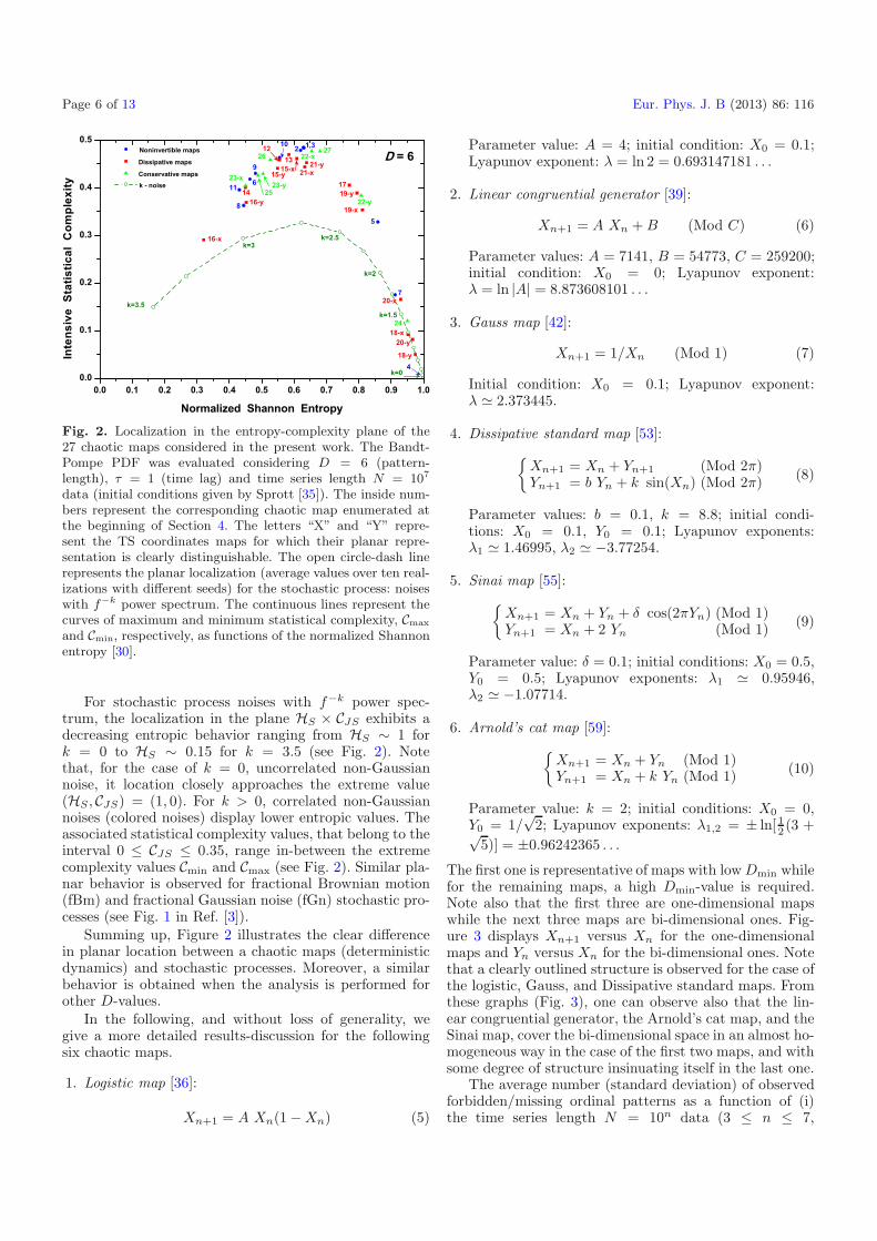
Figure 2 displays, for all the 27 chaotic maps here con-sidered, the entropy-complexity plane HS × CJS location.

Eur. Phys. J. B (2013) 86: 116 Page 5 of 13

Fig. 1. Dependence of the number of forbidden patterns ln N∗ as a function of the pattern-length D for the three kinds of maps:(a) noninvertible, (b) dissipative and, (c) conservative. Time series with N = 107 data (initial conditions given by Sprott [35])were considered. The pattern-lengths considered were Dmin ≤ D ≤ 8 and only chaotic maps with Dmin ≤ 7 in order to haveat least two points in the fit range. The numbers between parentheses represent the corresponding chaotic map enumerated atthe beginning of Section 4. The letters “X” and “Y” represent the TS coordinates maps for which their ln N∗-values are clearlydistinguishable.

The BP-PDF is evaluated for D = 6, τ = 1, and aTS-length N = 107 data (for initial conditions given bySprott [35]). In this graph, the given numbers representthe chaotic maps enumerated at the beginning of thissection. The letters “X” and “Y” represent the TS co-ordinates maps, for which their planar representations aredisplayed. We also present in this plot the planar local-ization for a stochastic process: noises with f−k powerspectrum [64] (0 ≤ k ≤ 3.5, with Δk = 0.25). The cor-responding values for these noises represent the averagevalue for ten realizations (N = 106 data), generated withdifferent seeds.

As a general behavior, all points corresponding to the27 chaotic maps are found in close vicinity to the max-imum complexity curve Cmax. In particular, for the caseof chaotic maps with 3 ≤ Dmin ≤ 5, they are localizedat a region of intermediate normalized Shannon entropyHS and high intensive statistical complexity CJS (closeto the curve of maximum complexity), in agreement withpreviously published results (see Fig. 1 in Ref. [3]). In-terestingly enough, localization in the entropy-complexityplane for chaotic maps with Dmin ≥ 6 tends to follow asimilar behavior, that is, high values of complexity butnow with HS ≥ 0.9.

Page 6 of 13 Eur. Phys. J. B (2013) 86: 116

Fig. 2. Localization in the entropy-complexity plane of the27 chaotic maps considered in the present work. The Bandt-Pompe PDF was evaluated considering D = 6 (pattern-length), τ = 1 (time lag) and time series length N = 107

data (initial conditions given by Sprott [35]). The inside num-bers represent the corresponding chaotic map enumerated atthe beginning of Section 4. The letters “X” and “Y” repre-sent the TS coordinates maps for which their planar repre-sentation is clearly distinguishable. The open circle-dash linerepresents the planar localization (average values over ten real-izations with different seeds) for the stochastic process: noiseswith f−k power spectrum. The continuous lines represent thecurves of maximum and minimum statistical complexity, Cmax

and Cmin, respectively, as functions of the normalized Shannonentropy [30].

For stochastic process noises with f−k power spec-trum, the localization in the plane HS × CJS exhibits adecreasing entropic behavior ranging from HS ∼ 1 fork = 0 to HS ∼ 0.15 for k = 3.5 (see Fig. 2). Notethat, for the case of k = 0, uncorrelated non-Gaussiannoise, it location closely approaches the extreme value(HS , CJS) = (1, 0). For k > 0, correlated non-Gaussiannoises (colored noises) display lower entropic values. Theassociated statistical complexity values, that belong to theinterval 0 ≤ CJS ≤ 0.35, range in-between the extremecomplexity values Cmin and Cmax (see Fig. 2). Similar pla-nar behavior is observed for fractional Brownian motion(fBm) and fractional Gaussian noise (fGn) stochastic pro-cesses (see Fig. 1 in Ref. [3]).

Summing up, Figure 2 illustrates the clear differencein planar location between a chaotic maps (deterministicdynamics) and stochastic processes. Moreover, a similarbehavior is obtained when the analysis is performed forother D-values.

In the following, and without loss of generality, wegive a more detailed results-discussion for the followingsix chaotic maps.

1. Logistic map [36]:

Xn+1 = A Xn(1 − Xn) (5)

Parameter value: A = 4; initial condition: X0 = 0.1;Lyapunov exponent: λ = ln 2 = 0.693147181 . . .

2. Linear congruential generator [39]:

Xn+1 = A Xn + B (Mod C) (6)

Parameter values: A = 7141, B = 54773, C = 259200;initial condition: X0 = 0; Lyapunov exponent:λ = ln |A| = 8.873608101 . . .

3. Gauss map [42]:

Xn+1 = 1/Xn (Mod 1) (7)

Initial condition: X0 = 0.1; Lyapunov exponent:λ � 2.373445.

4. Dissipative standard map [53]:{

Xn+1 = Xn + Yn+1 (Mod 2π)Yn+1 = b Yn + k sin(Xn) (Mod 2π) (8)

Parameter values: b = 0.1, k = 8.8; initial condi-tions: X0 = 0.1, Y0 = 0.1; Lyapunov exponents:λ1 � 1.46995, λ2 � −3.77254.

5. Sinai map [55]:{

Xn+1 = Xn + Yn + δ cos(2πYn) (Mod 1)Yn+1 = Xn + 2 Yn (Mod 1) (9)

Parameter value: δ = 0.1; initial conditions: X0 = 0.5,Y0 = 0.5; Lyapunov exponents: λ1 � 0.95946,λ2 � −1.07714.

6. Arnold’s cat map [59]:{

Xn+1 = Xn + Yn (Mod 1)Yn+1 = Xn + k Yn (Mod 1) (10)

Parameter value: k = 2; initial conditions: X0 = 0,Y0 = 1/

√2; Lyapunov exponents: λ1,2 = ± ln[12 (3 +√

5)] = ±0.96242365 . . .

The first one is representative of maps with low Dmin whilefor the remaining maps, a high Dmin-value is required.Note also that the first three are one-dimensional mapswhile the next three maps are bi-dimensional ones. Fig-ure 3 displays Xn+1 versus Xn for the one-dimensionalmaps and Yn versus Xn for the bi-dimensional ones. Notethat a clearly outlined structure is observed for the case ofthe logistic, Gauss, and Dissipative standard maps. Fromthese graphs (Fig. 3), one can observe also that the lin-ear congruential generator, the Arnold’s cat map, and theSinai map, cover the bi-dimensional space in an almost ho-mogeneous way in the case of the first two maps, and withsome degree of structure insinuating itself in the last one.

The average number (standard deviation) of observedforbidden/missing ordinal patterns as a function of (i)the time series length N = 10n data (3 ≤ n ≤ 7,

Eur. Phys. J. B (2013) 86: 116 Page 7 of 13

Fig. 3. Graphical representation for the 6 chaotic maps (initial conditions given by Sprott [35]) analyzed with more detail inthe text. The graphs display Xn+1 versus Xn for the one-dimensional maps: logistic, linear congruential generator, and Gauss,on the one hand, and Yn versus Xn for the bi-dimensional maps: dissipative standard, Sinai, and Arnold’s cat, on the otherhand.

Δn = 1); (ii) the pattern-length (embedding dimension)D (3 ≤ D ≤ 8, ΔD = 1), time lag τ = 1; (for ten differ-ent initial conditions) are listed in Table 1 for the abovesix chaotic maps. In the case of bi-dimensional chaoticmaps, the values for each one of the map’s coordinatesare detailed.

As expected, the results displayed in Table 1 do not de-pend (zero standard deviation) on the chaotic map’s initialconditions, if the true number of forbidden patterns canbe detected for the time series’ length considered. If suchconditions are not fulfilled for the maximum TS-lengthsconsidered, we also notice in Table 1 an overestimation ofthe number of forbidden ordinal patterns (some of themare missing patterns). However, the corresponding stan-dard error is quite low compared with the mean value,allowing us to take the numerical mean value 〈N∗〉 as rep-resentative of the number of forbidden ordinal patternscharacterizing the chaotic map.

In the case of the logistic map, inspection of Table 1makes it clear that forbidden ordinal patterns are observed

for all the pattern-lengths here considered. Thus, for thismap one has Dmin = 3. Note also that values of forbiddenordinal patterns N∗ are stable (constant, with zero stan-dard deviation) for most of the different time series lengthsconsidered by us. For the conjunction X0 = 0.1, D = 7 andN = 103, we detect N∗ = 4866 forbidden/missing pat-terns (some of these do not appear due to the short lengthof the pertinent time series), which reduces to N∗ = 4862forbidden patterns with zero standard deviation for TS-lengths with N = 104 up to 107 data. In this last case,such is the number of real forbidden patterns. Note alsothe exponential growth of forbidden ordinal patterns forincreasing values of the pattern-length D (see Fig. 1a).A similar situation is also observed for the rest of ourchaotic maps.

Table 1 allows one to conclude that the number ofmissing ordinal patterns tends to vanish as the time se-ries’ length grows, if the pattern-length considered isD < Dmin. We only start to find a non-zero numberof forbidden/missing ordinal patterns when considering

Page 8 of 13 Eur. Phys. J. B (2013) 86: 116

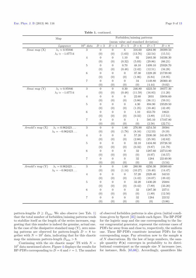
Table 1. Mean value of number of forbidden/missing ordinal patterns (standard deviation) for 10 different initial conditions, asa function of the chaotic time series length N for pattern-length D corresponding to the six chaotic maps analyzed with moredetail in the text.

Map Forbidden/missing patterns

(mean value and standard deviation)

Lyapunov 10n data D = 3 D = 4 D = 5 D = 6 D = 7 D = 8

Logistic map λ = ln 2 3 1 12 89 645.10 4869.90 39981.80

= 0.693147 . . . (0) (0) (0) (0.32) (2.42) (8.48)

4 1 12 89 645 4862 39906.80

(0) (0) (0) (0) (0) (0.92)

5 1 12 89 645 4862 39906

(0) (0) (0) (0) (0) (0)

6 1 12 89 645 4862 39906

(0) (0) (0) (0) (0) (0)

7 1 12 89 645 4862 39906

(0) (0) (0) (0) (0) (0)

Lineal congruential λ = ln |A| 3 0 0 0 167.10 4144.30 39344.20

generator = 8.873608 . . . (0) (0) (0) (9.46) (11.07) (3.68)

4 0 0 0 0 1182 32518.20

(0) (0) (0) (0) (13.71) (44.39)

5 0 0 0 0 341.80 23448.40

(0) (0) (0) (0) (3.12) (38.91)

6 0 0 0 0 279 21895

(0) (0) (0) (0) (0) (0)

7 0 0 0 0 279 21895

(0) (0) (0) (0) (0) (0)

Gauss map λ � 2.373445 3 0 0 4.80 330 4323.10 39420

(0) (0) (1.69) (19.75) (26.30) (16.63)

4 0 0 0 31.50 2305.60 34421.60

(0) (0) (0) (6.65) (41.01) (85.32)

5 0 0 0 0 340.70 20292

(0) (0) (0) (0) (20.59) (98.31)

6 0 0 0 0 1 4779.70

(0) (0) (0) (0) (0.82) (41.51)

7 0 0 0 0 0 121

(0) (0) (0) (0) (0) (7.51)

Dissipative standard λ1 � 1.46995 3 0 0 0.80 257.80 4252.80 39398.90

map (X) λ2 � −3.77254 (0) (0) (0.92) (16.40) (23.05) (16.07)

4 0 0 0 4.60 1578.20 33464.20

(0) (0) (0) (2.80) (36.66) (83.29)

5 0 0 0 0 35.50 13336.50

(0) (0) (0) (0) (5.60) (166.79)

6 0 0 0 0 0 871.50

(0) (0) (0) (0) (0) (27.73)

7 0 0 0 0 0 28.90

(0) (0) (0) (0) (0) (4.07)

Dissipative standard λ1 � 1.46995 3 0 0 0.10 223.90 4201.40 39364.80

map (Y) λ2 � −3.77254 (0) (0) (0.32) (12.81) (10.20) (8.10)

4 0 0 0 0 1130.90 32550.70

(0) (0) (0) (0) (52.30) (108.68)

5 0 0 0 0 1.20 7837.20

(0) (0) (0) (0) (1.23) (86.93)

6 0 0 0 0 0 3

(0) (0) (0) (0) (0) (1.56)

7 0 0 0 0 0 0

(0) (0) (0) (0) (0) (0)

Eur. Phys. J. B (2013) 86: 116 Page 9 of 13

Table 1. continued.

Map Forbidden/missing patterns

(mean value and standard deviation)

Lyapunov 10n data D = 3 D = 4 D = 5 D = 6 D = 7 D = 8

Sinai map (X) λ1 � 0.95946 3 0 0 6 316.60 4284.90 39399.50

λ2 � −1.07714 (0) (0) (1.63) (13.76) (22.54) (15.51)

4 0 0 1.10 92 2483.30 34336.30

(0) (0) (0.32) (5.03) (29.86) (66.21)

5 0 0 0.70 48.10 1499.10 25928.70

(0) (0) (0.48) (2.42) (12.51) (34.28)

6 0 0 0 37.30 1228.20 21739.80

(0) (0) (0) (1.06) (6.84) (18.95)

7 0 0 0 34 1149.80 20360.40

(0) (0) (0) (0) (4.44) (9.02)

Sinai map (Y) λ1 � 0.95946 3 0 0 0.30 246.80 4223.50 39377.30

λ2 � −1.07714 (0) (0) (0.48) (11.59) (16.83) (11.20)

4 0 0 0 22.60 2031 33856.60

(0) (0) (0) (3.86) (36.11) (59.31)

5 0 0 0 4.30 894.90 23529.50

(0) (0) (0) (1.25) (10.46) (42.49)

6 0 0 0 1.10 653.70 18621

(0) (0) (0) (0.32) (3.89) (17.51)

7 0 0 0 1 585.10 17107.80

(0) (0) (0) (0) (2.58) (22.71)

Arnold’s map (X) λ1 = 0.962423 . . . 3 0 0 1.80 276.90 4254.50 39384

λ2 = −0.962423 . . . (0) (0) (1.78) (8.16) (12.53) (9.19)

4 0 0 0 57.20 2330.30 34149.70

(0) (0) (0) (2.66) (25.50) (42.62)

5 0 0 0 32.10 1434.80 25726.50

(0) (0) (0) (0.32) (9.87) (41.79)

6 0 0 0 32 1287.60 22713.80

(0) (0) (0) (0) (0.97) (16.57)

7 0 0 0 32 1284 22149.90

(0) (0) (0) (0) (0) (3.54)

Arnold’s map (Y) λ1 = 0.962423 . . . 3 0 0 1.80 280.90 4256.30 39389.60

λ2 = −0.962423 . . . (0) (0) (1.14) (10.27) (18.40) (14.47)

4 0 0 0 57.20 2329.40 34153

(0) (0) (0) (4.42) (18.07) (49.42)

5 0 0 0 32.20 1430.20 25684

(0) (0) (0) (0.42) (7.89) (33.20)

6 0 0 0 32 1287.30 22711

(0) (0) (0) (0) (1.89) (12.50)

7 0 0 0 32 1284 22152

(0) (0) (0) (0) (0) (3.86)

pattern-lengths D ≥ Dmin. We also observe (see Tab. 1)that the total number of forbidden/missing patterns tendsto stabilize itself as the length of the series increases, sug-gesting that this number is indeed the genuine, actual one.In the case of the dissipative standard map (Y), zero miss-ing patterns are observed for pattern-length D = 8 to-gether with N = 107 data, indicating that for this chaoticmap the minimum pattern-length Dmin > 8.

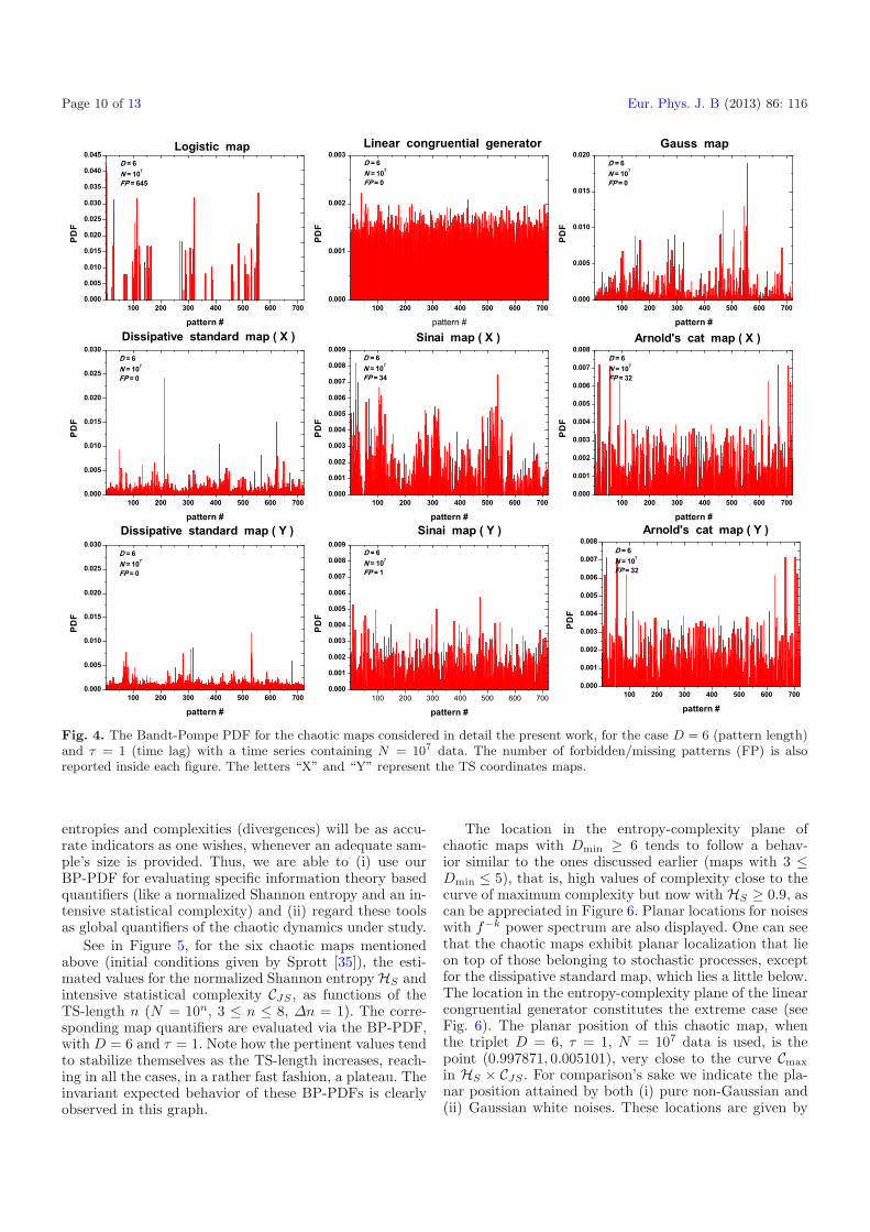
Continuing with the six chaotic maps’ TS with N =107 data mentioned above, Figure 4 displays the results forBP-PDFs corresponding to D = 6 and τ = 1. The number

of observed forbidden patterns is also given (initial condi-tions given by Sprott [35]) inside each figure. The BP-PDFfor the logistic map and the one corresponding to the lin-ear congruential generator, represent the extreme cases ofPDFs far away from and close to, respectively, the uniformone. These BP-PDFs constitute invariant PDFs for thecorresponding maps. Pay attention now to the sample xof N observations. By the law of large numbers, the sam-ple quantity Ψ(x) converges in probability to its distri-butional counterpart as the sample size N increases (see,for instance, Refs. [65,66]). Accordingly, quantifiers like

Page 10 of 13 Eur. Phys. J. B (2013) 86: 116

Fig. 4. The Bandt-Pompe PDF for the chaotic maps considered in detail the present work, for the case D = 6 (pattern length)and τ = 1 (time lag) with a time series containing N = 107 data. The number of forbidden/missing patterns (FP) is alsoreported inside each figure. The letters “X” and “Y” represent the TS coordinates maps.

entropies and complexities (divergences) will be as accu-rate indicators as one wishes, whenever an adequate sam-ple’s size is provided. Thus, we are able to (i) use ourBP-PDF for evaluating specific information theory basedquantifiers (like a normalized Shannon entropy and an in-tensive statistical complexity) and (ii) regard these toolsas global quantifiers of the chaotic dynamics under study.

See in Figure 5, for the six chaotic maps mentionedabove (initial conditions given by Sprott [35]), the esti-mated values for the normalized Shannon entropy HS andintensive statistical complexity CJS , as functions of theTS-length n (N = 10n, 3 ≤ n ≤ 8, Δn = 1). The corre-sponding map quantifiers are evaluated via the BP-PDF,with D = 6 and τ = 1. Note how the pertinent values tendto stabilize themselves as the TS-length increases, reach-ing in all the cases, in a rather fast fashion, a plateau. Theinvariant expected behavior of these BP-PDFs is clearlyobserved in this graph.

The location in the entropy-complexity plane ofchaotic maps with Dmin ≥ 6 tends to follow a behav-ior similar to the ones discussed earlier (maps with 3 ≤Dmin ≤ 5), that is, high values of complexity close to thecurve of maximum complexity but now with HS ≥ 0.9, ascan be appreciated in Figure 6. Planar locations for noiseswith f−k power spectrum are also displayed. One can seethat the chaotic maps exhibit planar localization that lieon top of those belonging to stochastic processes, exceptfor the dissipative standard map, which lies a little below.The location in the entropy-complexity plane of the linearcongruential generator constitutes the extreme case (seeFig. 6). The planar position of this chaotic map, whenthe triplet D = 6, τ = 1, N = 107 data is used, is thepoint (0.997871, 0.005101), very close to the curve Cmax

in HS × CJS . For comparison’s sake we indicate the pla-nar position attained by both (i) pure non-Gaussian and(ii) Gaussian white noises. These locations are given by

Eur. Phys. J. B (2013) 86: 116 Page 11 of 13

Fig. 5. Variation of the information theory quantifiers, normalized Shannon entropy (H) and intensive statistical complexity (C)as a function of the time series length N = 10n (3 ≤ n ≤ 7), evaluated with PDF-Bandt and Pompe, with D = 6 and τ = 1, forthe six chaotic maps analyzed with more detail in the text. The letters “X” and “Y” represent the TS coordinates maps.

the points (0.999943, 0.000134) and (0.999945, 0.000130),respectively. We note a clear difference between the pla-nar localization of either a chaotic map or a stochasticprocess.

5 Conclusions

We reviewed in the present work the characterization ofsome chaotic maps’ TS from the viewpoint of the permu-tation Bandt-Pompe PDFs. We considered “local” char-acteristics of the components of this PDF, the so-calledforbidden/missing ordinal patterns, as well as quantifiersderived from information theory (normalized Shannon en-tropy, intensive statistical complexity, entropy-complexityplane) that make use of all the components of the PDF,and are accordingly called “global”.

If forbidden ordinal patterns are observed in a finitedata time series, they exhibit an exponential growth forfinite pattern-lengths (embedding dimension) D. This be-havior could be regarded as the hallmark of determinism

in a time series. We have shown that even when the pres-ence of forbidden patterns can be associated to a chaoticdynamics, a minimum pattern-length, Dmin must be con-sidered in order to observe this phenomenon. This is a factthat has not been pointed out before. In fact, we couldnot find any reference to Dmin in the published literature.Moreover, we infer from it that, using the Band-Pompemethodology, the existence of this quantity was not con-sidered in classifying time series as either deterministic orstochastic. Note that ignoring the existence (discoveredby us here) of this minimal pattern-length could lead towrong interpretations.

Per contra, in the case of quantifiers evaluated makinguse of the whole BP-PDF, for fixed values of the pattern-length (embedding dimension) D and time lag τ , a specificbehavior is observed for the case of chaotic dynamics. Lo-calization in the entropy-complexity plane HS × CJS , forthe case of chaotic maps, closely approaches the limitingcurve of maximum statistical complexity Cmax. Note thata similar behavior is still observed when chaotic maps’TS are contaminated with small or moderate amount of

Page 12 of 13 Eur. Phys. J. B (2013) 86: 116

Fig. 6. Localization in the entropy-complexity plane of the6 chaotic maps (initial conditions given by Sprott [35]) ana-lyzed with more detail in the text. The Bandt-Pompe PDF wasevaluated considering D = 6 (pattern-length), τ = 1 (time lag)and TS-length N = 107 data. The inside numbers representthe corresponding chaotic map enumerated at the beginningof Section 4. The letters “X” and “Y” represent the TS co-ordinates maps for which their planar representation is clearlydistinguishable. The open circle-dash line represents the planarlocalization (average values over ten realizations with differentseeds) for the stochastic process: noises with f−k power spec-trum. The continuous lines represent the curves of maximumand minimum statistical complexity, Cmax and Cmin, respec-tively, as functions of the normalized Shannon entropy [30].

additive uncorrelated or correlated noise [15,16]. Basedon such behavior, we conclude that a more “robust” dis-tinction between deterministic and stochastic dynamics isgiven via the present TS-treatment, that takes into ac-count the whole of the permutation Bandt-Pompe PDF(global quantifier), and not just part of it.

O.A. Rosso gratefully acknowledges support from CNPq, Fel-lowship, Brazil. F. Olivares is supported by a Fellowship of theChilean Government, CONICYT. This work was partially sup-ported by the projects PIP1177 and PIP112-200801-01420 ofCONICET (Argentina), and the projects FIS2008-00781/FIS(MICINN)-FEDER (EU) (Spain, EU).

References

1. C. Bandt, B. Pompe, Phys. Rev. Lett. 88, 174102 (2002)2. M. Zanin, L. Zunino, O.A. Rosso, D. Papo, Entropy 14,

1553 (2012)3. O.A. Rosso, H.A. Larrondo, M.T. Martın, A. Plastino,

M.A. Fuentes, Phys. Rev. Lett. 99, 154102 (2007)4. M. Zanin, Chaos 18, 013119 (2008)5. J.M. Amigo, S. Zambrano, M.A.F. Sanjuan, Europhys.

Lett. 79, 50001 (2007)6. J.M. Amigo, Permutation complexity in dynamical systems

(Springer-Verlag, Berlin, 2010)7. O.A. Rosso, C. Masoller, Phys. Rev. E 79, 040106(R)

(2009)

8. O.A. Rosso, C. Masoller, Eur. Phys. J. B 69, 37 (2009)9. P.M. Saco, L.C. Carpi, A. Figliola, E. Serrano, O.A. Rosso,

Physica A 389, 5022 (2010)10. K. Keller, M. Sinn, Physica A 356, 114 (2005)11. M.C. Soriano, L. Zunino, L. Larger, I. Fischer, C.R.

Mirasso, Opt. Lett. 36, 2212 (2011)12. M.C. Soriano, L. Zunino, O.A. Rosso, I. Fischer, C.R.

Mirasso, IEEE J. Quantum Electron. 47, 252 (2011)13. L. Zunino, M.C. Soriano, I. Fischer, O.A. Rosso, C.R.

Mirasso, Phys. Rev. E 82, 046212 (2010)14. L. Zunino, M.C. Soriano, O.A. Rosso, Phys. Rev. E 86,

046210 (2012)15. O.A. Rosso, L.C. Carpi, P.M. Saco, M. Gomez Ravetti, A.

Plastino, H.A. Larrondo, Physica A 391, 42 (2012)16. O.A. Rosso, L.C. Carpi, P.M. Saco, M. Gomez Ravetti,

H.A. Larrondo, A. Plastino, Eur. Phys. J. B 85, 419 (2012)17. J.M. Amigo, L. Kocarev, J. Szczepanski, Phys. Lett. A

355, 27 (2006)18. J.M. Amigo, S. Zambrano, M.A.F. Sanjuan, Europhys.

Lett. 83, 60005 (2008)19. L.C. Carpi, P.M. Saco, O.A. Rosso, Physica A 389, 2020

(2010)20. H. Wold, A Study in the Analysis of Stationary Time Se-

ries (Almqvist and Wiksell, Upsala, 1938)21. J. Kurths, H. Herzel, Physica D 25, 165 (1987)22. S. Cambanis, C.D. Hardin, A. Weron, Probab. Theory

Related Fields 79, 1 (1988)23. D.P. Feldman, J.P. Crutchfield, Phys. Lett. A 238, 244

(1998)24. D.P. Feldman, C.S. McTague, J.P. Crutchfield, Chaos 18,

043106 (2008)25. P.W. Lamberti, M.T. Martın, A. Plastino, O.A. Rosso,

Physica A 334, 119 (2004)26. R. Lopez-Ruiz, H.L. Mancini, X. Calbet, Phys. Lett. A

209, 321 (1995)27. C. Shannon, W. Weaver, The Mathematical theory of com-

munication (University of Illinois Press, Champaign, 1949)28. I. Grosse, P. Bernaola-Galvan, P. Carpena, R. Roman-

Roldan, J. Oliver, H.E. Stanley, Phys. Rev. E 65, 041905(2002)

29. A.R. Plastino, A. Plastino, Phys. Rev. E 54, 4423 (1996)30. M.T. Martın, A. Plastino, O.A. Rosso, Physica A 369, 439

(2006)31. O.A. Rosso, L. De Micco, H. Larrondo, M.T. Martın, A.

Plastino, Int. J. Bifur. Chaos 20, 775 (2010)32. L. Zunino, M. Zanin, B.M. Tabak, D.G. Perez, O.A. Rosso,

Physica A 389, 1891 (2010)33. L. Zunino, B.M. Tabak, F. Serinaldi, M. Zanin, D.G. Perez,

O.A. Rosso, Physica A 390, 876 (2011)34. L. Zunino, A. Fernandez Bariviera, M.B. Guercio, L.B.

Martinez, O.A. Rosso, Physica A 391, 4342 (2012)35. J.C. Sprott, Chaos and time series analysis (Oxford

University Press, New York, 2003)36. R. May, Nature 261, 45 (1976)37. S.H. Strogatz, Nonlinear dymanics and chaos with appli-

cations to physics, biology, chemistry, and engineering(Addison-Wesley-Longman, Reading, 1994)

38. R.L. Devaney, An introduction to chaotic dynamical sys-tems, 2nd edn. (Addison-Wesley, Redwood City, 1989)

39. D.E. Knuth, Sorting and searching, Vol. 3 of The artof computer programming, 3rd edn. (Addison-Wesley-Longman, Reading, 1997)

Eur. Phys. J. B (2013) 86: 116 Page 13 of 13

40. W. Zeng, M. Ding, J. Li, Chinese Phys. Lett. 2, 293(1985)

41. W. Ricker, J. Fish. Res. Board Canada 11, 559 (1954)42. M.A. van Wyk, W. Steeb, Chaos in electronics (Kluwer,

Dordrecht, 1997)43. C. Beck, F. Schlogl, Thermodynamics of chaotics systems

(Cambridge University Press, New York, 1995)44. A. Potapov, M.K. Ali, Phys. Lett. A 277, 310 (2000)45. R. Shaw, Z. Naturforsch. A 36, 80 (1981)46. V.I. Arnold, Am. Math. Soc. Transl. Ser. 46, 213 (1965)47. M. Henon, Commun. Math. Phys. 50, 69 (1976)48. R. Lozi, J. Phys. 39, 9 (1978)49. D.G. Aronson, M.A. Chory, G.R. Hall, R.P. McGehee,

Commun. Math. Phys. 83, 304 (1982)50. H.E. Nusse, J.A. Yorke, Dynamics: numerical explorations

(Springer, New York, 1994)51. R.R. Whitehead, N. Macdonald, Physica D 13, 401

(1984)52. P.J. Holmes, Philos. Trans. Roy. Soc. London Ser. A 292,

419 (1979)53. G. Schmidt, B.H. Wang, Phys. Rev. A 32, 2994 (1985)54. E. Ikeda, Opt. Commun. 30, 257 (1979)

55. Ya. G. Sinai, Russian Math. Surv. 27, 21 (1972)56. J.R. Beddington, C.A. Free, J.H. Lawton, Nature 255, 58

(1975)57. B.V. Chirikov, Phys. Rep. 52, 273 (1979)58. M. Henon, Quart. Appl. Math. 27, 291 (1969)59. V.I. Arnold, A. Avez, Ergodic problems of classical me-

chanics (Benjamin, New York, 1968)60. R.L. Devaney, Physica D 10, 387 (1984)61. A.A. Chernikov, R.Z. Sagdeev, G.M. Zaslavsky, Phys.

Today 41, 27 (1988)62. E.N. Lorenz, The essence of chaos (University of

Washington Press, Seattle, 1993)63. B. Nagy, J.D. Farmer, J.E. Trancik, J.P. Gonzales,

Technol. Forecast. Soc. Change 78, 1356 (2011)64. H.A. Larrondo, Matlab program: noisefk.m (2012),

http://www.mathworks.com/matlabcentral/

fileexchange/35381

65. S.I. Resnick, A Probability Path (Birkhauser, Boston,1999)

66. C.F. Manski, Analog estimation methods in economet-rics, in Monographs on Statistics and Applied Probability(Chapman & Hall, New York, 1988), Vol. 39