Characteristics of Tropical Cyclones in Atmospheric ...suzana/papers/camargo_et_al.pdf · Characteristics of Tropical Cyclones in Atmospheric General Circulation Models ... and their

Characteristics of Tropical Cyclones in Atmospheric

General Circulation Models

SUZANA J. CAMARGO∗, ANTHONY G. BARNSTON, AND STEPHENE. ZEBIAK

International Research Institute for Climate Prediction,

The Earth Institute of Columbia University

Lamont Campus, PO Box 1000, Palisades, NY 10964-8000

April 16, 2004

Abstract

The properties of tropical cyclones in three low-resolution atmospheric general circulation

models (AGCMs) are discussed. The models are forced by prescribed, observed sea surface

temperatures over a period of 40 years, and their simulations of tropical cyclone activity are

compared with observations. The model cyclone characteristics considered include genesis po-

∗email:[email protected]

1

sition, number of cyclones per year, seasonality, accumulated cyclone energy, track locations,

and number of storm days. Correlations between model and observed interannual variations of

these characteristics are evaluated. The models are found able to reproduce the basic features

of observed tropical cyclone behavior such as seasonality, general location and interannual

variability, but with identifiable biases. A bias correction is applied to the tropical cyclone

variables of the three models. The three AGCMs have different levels of realism in simu-

lating different aspects of tropical cyclone activity in different ocean basins. Some strengths

and weaknesses in simulating certain tropical cyclone activity variables are common to the

three models, while others are unique to each model and/or basin. The overall skill of the

models in reproducing observed interannual variability of tropical cyclone variables is roughly

comparable to that of statistical models.

1. Introduction

The possibility of using dynamical climate models to forecast seasonal tropical cyclone activity has

been explored by various authors (e.g. Bengtsson et al. (1982); Vitart et al. (1997)). Although low-

resolution (2◦− 3◦) climate general circulation models are not adequate for forecasts of individual

cyclones, they can have skill in forecasting seasonal tropical cyclone activity (Bengtsson, 2001).

Presently, experimental dynamical forecasts of tropical cyclone activity are produced by several

2

centers, including the International Research Institute for Climate Prediction (IRI) (IRI, 2004)

and the European Centre for Medium-Range Weather Forecasts (ECMWF) (Vitart and Stockdale,

2001). The effectiveness of dynamical climate models for forecasting tropical cyclone landfall

over Mozambique has recently been analyzed by Vitart et al. (2003). Routine seasonal forecasts of

tropical cyclone frequency in the Atlantic sector are produced using statistical methods by different

institutions (Gray et al., 1993, 1994; CPC, 2004; TSR, 2004). Statistical seasonal forecasts of

tropical cyclone frequency are also issued for the western North Pacific, eastern North Pacific and

Australian sectors (Chan et al., 1998; Liu and Chan, 2003; CPC, 2004; TSR, 2004).

A better understanding of the performance of different low-resolution atmospheric general cir-

culation models (AGCMs) under ideal circumstances of forcing by “perfect” (observed) sea sur-

face temperature (SST), is helpful in assessing the skill of these dynamical forecasts. In this paper,

some basic characteristics of model tropical cyclones are examined in multidecadal simulations

from three low-resolution global AGCMs. Previous studies of tropical cyclones in low-resolution

AGCMs focused on single integrations (Bengtsson et al., 1995) or ensembles of a single model

(e.g. Vitart et al. (1997)) in a restricted time period (9 years in Vitart et al. (1997) and Vitart and

Stockdale (2001)). Here we evaluate the performance of three AGCMs in simulating tropical cy-

clone activity over a longer period (40 years) and for larger ensemble sets (9 to 24 members per

model).

3

Tropical cyclones in low-resolution AGCMs have been found to have characteristics similar

to those observed (e.g. Manabe et al. (1970)). The intensity of these model cyclones is much

lower, and their spatial scale larger, than their observed counterparts due to the low-resolution

(Bengtsson et al., 1995; Vitart et al., 1997). The climatology, structure and interannual variability

of model tropical cyclones have been examined (Bengtsson et al., 1982, 1995; Vitart et al., 1997),

as well as their relation to large scale circulation (Vitart et al., 1999) and SST variability (Vitart

and Stockdale, 2001). The characteristics of model tropical cyclone formation over the western

North Pacific have also been studied (Camargo and Sobel, 2004). In many cases, the spatial and

temporal distributions of model tropical cyclones are found to be similar to those of observed

tropical cyclones (Bengtsson et al., 1995; Vitart et al., 1997; Camargo and Zebiak, 2002).

There are two primary methods of using AGCMs to forecast tropical cyclone activity. One

approach is to analyze large-scale variables known to affect tropical cyclone activity (Ryan et al.,

1992; Watterson et al., 1995; Thorncroft and Pytharoulis, 2001). Another approach, and the one

used here, is to detect and track cyclone-like structures in AGCMs and coupled ocean-atmosphere

models (Manabe et al., 1970; Bengtsson et al., 1982; Krishnamurti, 1988; Krishnamurti et al.,

1989; Broccoli and Manabe, 1990; Wu and Lau, 1992; Haarsma et al., 1993; Bengtsson et al.,

1995; Tsutsui and Kasahara, 1996; Vitart et al., 1997; Vitart and Stockdale, 2001; Camargo and

Zebiak, 2002). The last approach has also been used in studies of possible changes in tropical

4

cyclone intensity due to global climate change both using AGCMs (Bengtsson et al., 1996; Sugi

et al., 2002) and regional climate models (Walsh and Ryan, 2000).

The nature of tropical cyclone activity in AGCMs depends on various characteristics of the

models, such as physical parametrizations and circulation. Therefore, the analysis of the tropical

cyclone activity in different AGCMs provides a different diagnostic of the strengths and weak-

nesses of these AGCMs and could be used to improve future versions of these models.

This paper is organized as follows. A brief discussion of the data and methodology is given

in section 2. We examine global model climatologies of several parameters of tropical cyclone

activity in section 3, and the characteristics and skills of simulated interannual variability of these

parameters by individual basins in section 4. Conclusions are given in section 5. A more detailed

version of this paper appears as a Technical Report in Camargo et al. (2004a).

2. Data and methodology

The AGCMs used in this study are ECHAM3.6 (here denoted ECHAM3), ECHAM4.5 (denoted

ECHAM4), and NSIPP-1 (denoted NSIPP). The first two models were developed at the Max-

Planck Institute for Meteorology, Hamburg, Germany (Model User Support Group, 1992; Roeck-

ner et al., 1996) and the third model was developed at NASA/Goddard in Maryland, USA (NASA

5

Seasonal to Interannual Prediction Project); (Suarez and Takacs, 1995). The model integrations

used in this study were performed using observed sea surface temperature with the number of

ensemble members, period and output frequency as shown in Table 1. The resolution of both

ECHAM models is T42 (2.81◦)while the NSIPP model has resolution of2.5◦×2◦ longitude/latitude.

These resolutions are used in IRI operational seasonal forecasts (Mason et al., 1999; Goddard

et al., 2001, 2003; Barnston et al., 2003). The model integrations of both ECHAM models were

performed at IRI, while the NSIPP integrations were performed at NASA/Goddard.

Both ECHAM models have a parametrization of cumulus convection based on the bulk mass

flux concept of Tiedtke (1989); however a modified version of this parametrization was used in

ECHAM4 (Roeckner et al., 1996). The NSIPP model convection parametrization uses the relaxed

Arakawa-Shubert scheme (Moorthi and Suarez, 1992).

Although a longer period of integrations for some of the models is available, we restrict the

analysis to the common period of 1961-2000. The observational data used are from the Best Track

datasets. The Southern Hemisphere, Indian Ocean and western North Pacific data are from the

Joint Typhoon Warning Center (JTWC, 2004), while the eastern North Pacific and Atlantic data

are from the National Hurricane Center (NHC, 2004). From the observed datasets, only tropical

cyclones with tropical storm or typhoon intensity are considered for the model comparison, i.e.

tropical depressions (not named) are not included.

6

To obtain representative tropical cyclone frequency values in AGCMs, objective algorithms

for detection and tracking of individual model tropical cyclones were developed (Camargo and

Zebiak, 2002), based substantially on prior studies (Vitart et al., 1997; Bengtsson et al., 1995).

The algorithm has two parts. In the detection part, storms that meet environmental and duration

criteria are identified. A model tropical cyclone is identified when chosen dynamical and ther-

modynamical variables exceed thresholds determined from observed tropical storm climatology.

Basin and model dependence in detection algorithms yields better simulation of the seasonal cycle

and interannual variability (Camargo and Zebiak, 2002). In the tracking part, disturbance tracks are

obtained from the vorticity centroid, which defines the center of the tropical cyclone, and relaxed

criteria. The detection and tracking algorithms detailed in that study have been applied to more lo-

calized tropical cyclone studies using regional climate models and reanalysis data (Landman et al.,

2002; Camargo et al., 2002), and are applied to the AGCMs used in the present study.

The definitions of the basins used here for the formation regions of the tropical cyclones are

shown in Fig. 1. When the whole life cycle of the cyclones is considered, the poleward latitude

limit is eliminated. Model biases in the mean and the distributional features of the tropical cyclone

activity variables analyzed are treated individually by model and by basin. The distribution of the

observed variable per year over the 40 year period is compared with the model distributions, using

all model ensemble members. Values corresponding to each 10th percentile are identified across

7

the two distributions, and the model values are “corrected” to the observed values. Values between

decile locations in the models are treated using bilinear interpolation, and extrapolation is applied

for the two tails (< 10 and> 90 percentiles). The resulting modified model distributions not only

have means and standard deviations very similar to those observed, but their higher moments also

become similar (except for possibly the extreme tails). The broad features of the patterns of the

models’ interannual variability are not appreciably affected by the bias correction. In most figures,

the results shown are not bias-corrected; figures with bias-corrected variables are identified in their

captions.

3. Model climatology

It is fundamental to know whether the models generate tropical cyclones in the regions and during

the seasons in which they are observed in nature. In this section we examine model climatologies

of genesis location, tracks, intensities and lifetimes.

a. Genesis location

In Fig. 2 the locations of tropical cyclone formation from one selected ensemble member of each

model are shown for the 1961-2000 period, along with the observed first positions. Though only

8

one of the ensemble members is shown, characteristics are sufficiently representative of the same

analysis for the ensemble mean. The three models have differing biases in location and amount

of tropical cyclone formation. However, all models are seen to have deficient formation in the

Atlantic basin–particularly in the Caribbean and Gulf of Mexico. The models form a few tropical

cyclones over land, as for example in ECHAM3 over western Africa1.

The distribution of first positions, calculated using all ensemble realizations of the models,

is expressed in terms of a frequency of storm genesis for each4◦ latitude or longitude interval,

normalized by the number of years (40) and number of ensemble members for each model (Fig. 3).

The zonal and meridional averages indicate a clear overall deficit in number of model cyclones

formed.

Fig. 3(a) shows an equatorward bias in all models’ tropical cyclone formation, with maximum

between8◦ and12◦ from the equator and a rapid falloff with increasing latitude. The observed

maximum occurs at12◦, with a more gradual decrease with latitude, especially in the north At-

lantic. The excess of cyclone formation near the equator occurs mainly in the Indian Ocean and

Central Pacific in the two ECHAM models, and in the Maritime Continent in the NSIPP model.

Figure 3(b) shows an eastward bias of both ECHAM models in the western Pacific, a bias not

found in the NSIPP model. Also evident is the marked deficiency of model cyclones formed over

1Our interpretation is that in ECHAM3 these represent easterly waves, which are mixed with (and indistinguishablefrom) the model’s low intensity tropical cyclones.

9

the eastern Pacific and Atlantic. ECHAM4 has the most realistic number of tropical cyclones in the

western North Pacific. While ECHAM3 has the most realistic density of tropical cyclone formation

in the Indian Ocean, it occurs mainly near the equator rather than in two separate bands on either

side of the equator. The NSIPP model has a realistic formation concentration near the Maritime

continent and Australia, as well as between Madagascar and Africa–the latter being weak in the

two ECHAM models. None of the models forms tropical cyclones over the South Atlantic, which

did occur in numerous previous studies (Broccoli and Manabe, 1990; Wu and Lau, 1992; Haarsma

et al., 1993; Tsutsui and Kasahara, 1996; Vitart et al., 1997).

The correspondences between the model and observed spatial distributions of formation loca-

tion was quantified using spatial correlation, mean square error, and the Kolmogorov-Smirnov test

(Sheskin, 2000). The NSIPP model has the highest global spatial correlation, while ECHAM4 has

the lowest mean square error. All three models are more skillful in the Southern than Northern

Hemisphere, due to their ability to roughly reproduce formation in the southern Indian and west-

ern South Pacific oceans. The Kolmogorov-Smirnov tests estimate distributional differences after

normalization for amplitude, and yield consistent results.

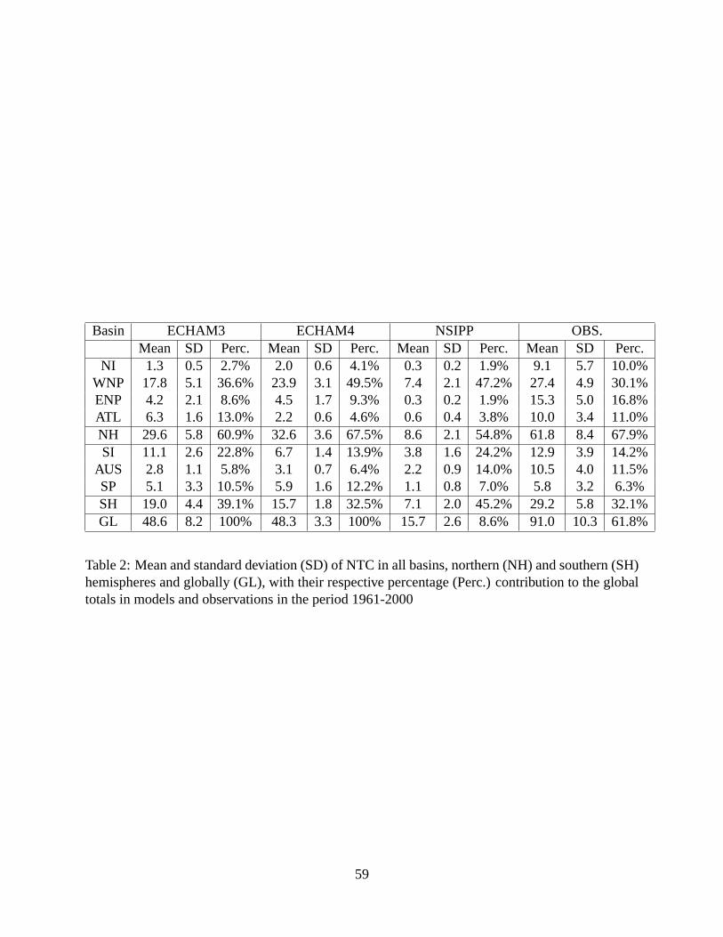
The mean and standard deviation of the number of tropical cyclones (NTC) per year in the

models and in observations are shown in table 2 for each ocean basin, each hemisphere and the

globe. The mean number of observed named tropical cyclones per year in the period 1961-2000

10

is 91.0. The ECHAM3 and ECHAM4 models’ ensemble means are approximately half of this

value, while the NSIPP model’s percentage is only17%. In observations, on average68% of the

total NTC are in the Northern Hemisphere and32% are in the Southern Hemisphere. All models

correctly produce more tropical cyclones in the Northern than Southern Hemisphere. The ratio

in ECHAM4 is very close to that observed, while in ECHAM3 and NSIPP the proportion in the

Southern Hemisphere is somewhat larger.

In observations, the western North Pacific has the highest fraction of the global NTC, averaging

27.4 cyclones per year, or30% of the global total (Table 2). All models reproduce this feature, but

with an even higher contribution to the global total, ranging from36.6% (ECHAM3) to 49.5%

(ECHAM4). The eastern North Pacific has the second highest NTC in observations with16.8%.

However, all three models produce proportionally few tropical cyclones there, ranging from1.9%

(NSIPP) to9.3% (ECHAM4). The low resolution is likely one reason for deficient performance in

this basin, as noted by Vitart et al. (1997) in the GFDL AGCM. A large percentage of the eastern

Pacific tropical cyclones are formed as easterly waves coming from the Atlantic cross the Central

America mountainous region (see e.g. Avila et al. (2003); Franklin et al. (2003)), which is poorly

represented in low-resolution AGCMs.

The Atlantic has very few tropical cyclones in the ECHAM4 and NSIPP models (Table 2).

The ECHAM3 model is active in the Atlantic with13% of the global NTC, compared with11%

11

in the observations (some, however, form over land in western Africa). In contrast, in ECHAM4

and NSIPP form most Atlantic tropical cyclones in the Caribbean region. The region with most

observed tropical cyclones in the Southern Hemisphere is the South Indian Ocean, followed by the

Australian region and the South Pacific. The only model whose NTC in the Southern Hemisphere

has this order is the NSIPP model; in ECHAM3 and ECHAM4 the contribution from the South

Pacific is higher than from the Australian region. This is analogous to, but less severe than, a bias

of these models in forming tropical cyclones too far east in the western North Pacific. ECHAM3

also has a disproportionate fraction of tropical cyclones forming between 70E and 100E in the

South Indian Ocean. The three models are deficient in cyclone formation around Australia, with

an unrealistic minimum from 100E to 150E (Fig. 3(b)).

b. Tracks, lifetimes and intensities

In addition to frequency and geographical distribution of model tropical cyclone genesis, we look

into the life cycle aspects of cyclone behavior: tracks, intensities, and lifetimes.

Fig. 4 shows all the tropical cyclone tracks2 in one of the ensemble members of each of the

models and in observations for the years 1993-1995. While the tracks vary among ensemble mem-

2Due to the low resolution, the tropical cyclone tracks are not as smooth as the observed ones, as the definedcenter of the tropical cyclone must “jump” from one grid point to another and the incremental distance is usually largecompared to that observed.

12

bers, one ensemble member over a small number of years lacking an ENSO extreme provides an

adequate sampling of the typical properties of the tracks.

In Vitart et al. (1997), the tropical cyclone tracks in the GFDL GCM were found to be located

somewhat more poleward, and to be shorter, than the observed tracks. A poleward tendency is

not evident in the AGCMs analyzed here (Fig. 4). This could be due to the differing tracking

algorithms used here. In Vitart et al. (2003), the algorithm was slightly modified and applied to

a different AGCM; this modification improved the realism of the tropical cyclone tracks. The

different characteristics of AGCM tracks could be due to model differences and/or to the tracking

algorithms.

In observations, the tropical cyclone tracks in the Southern Hemisphere are confined to a belt

between10◦S and40◦S with occasional observed excursions south of40◦S (Fig. 4). In both

ECHAM3 and ECHAM4 many tropical cyclones reach latitudes as far south as50◦S. On the

other hand, the NSIPP model’s tracks are shorter than those observed.

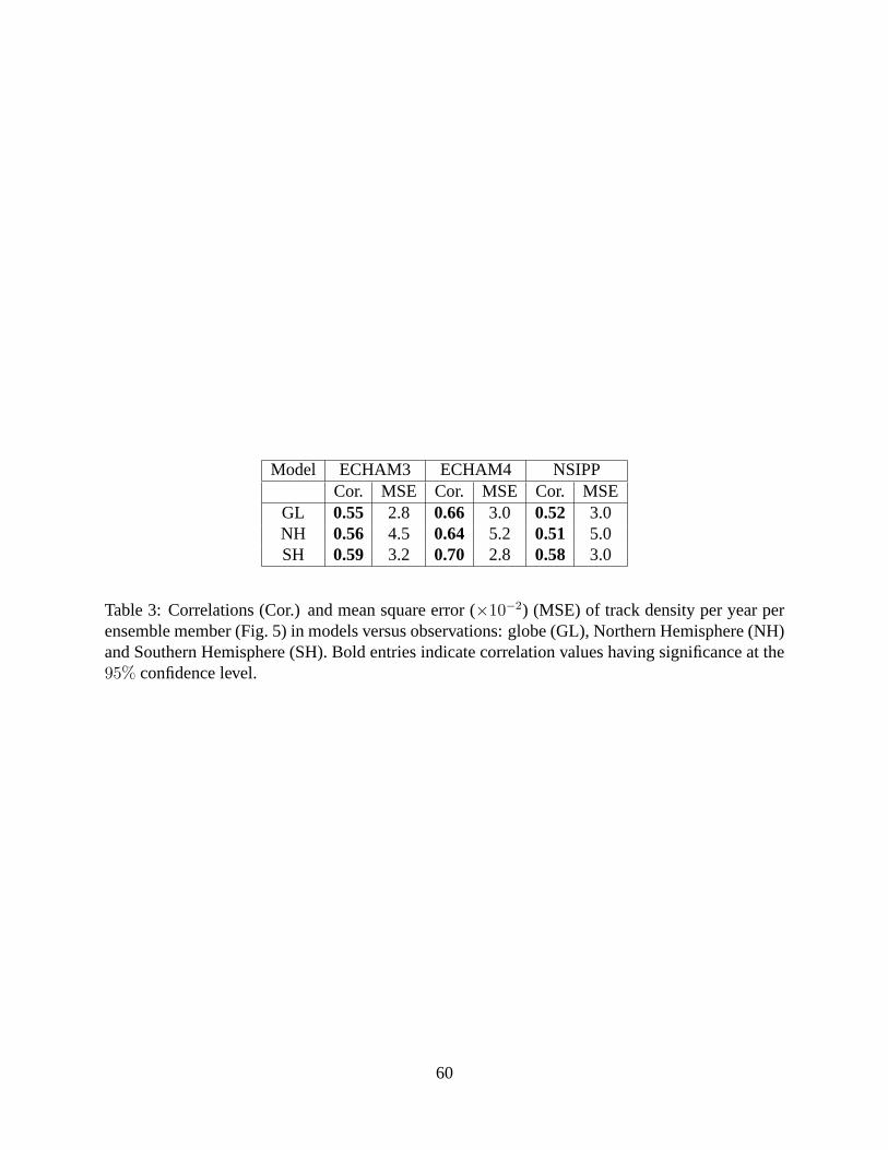
A more comprehensive view of the density of tracks is provided in Fig. 5. The track density

is shown as the number of track positions per4◦ latitude and longitude per year and per ensemble

member. The correspondence between the observed track density pattern with each model is sum-

marized in Table 3 using spatial correlation and mean square error, for each hemisphere and for

the globe. The ECHAM4 model has the highest spatial correlations, and all models have slightly

13

larger correlation coefficients in the Southern than in the Northern Hemisphere. Globally and in the

Northern Hemisphere, ECHAM3 has the smallest mean square error. The Kolmogorov-Smirnov

test (not shown) basically corroborates these findings. The NSIPP track density is less realistic

than its genesis location. This is related to its tracks being shorter than the observed tracks (Fig.

4c).

In the North Indian Ocean, the ECHAM4 and NSIPP models have a relative maximum of

track density in the Bay of Bengal, similar to the observations (Fig. 5). However, all models are

generally deficient of tracks in the North Indian Ocean. In the Arabian Sea, the ECHAM4 model

has a bias of too many landfalling cyclones on the Arabian Peninsula (Oman).

The general lack of tropical cyclone activity in the NSIPP model in the Southern Hemisphere

can also be seen in the track density pattern (Fig. 5), with the exception of an excess of activity

in the equatorial Indonesian region. Both ECHAM3 and ECHAM4 tend to have too much cyclone

activity far east of Australia, well east of the dateline, with a relative lack of tracks near Australia.

The NSIPP model has a realistic track density pattern in the Mozambique channel and southeast

African coast.

The large domains used in Table 3 may mask substantial but smaller scale features of the

pattern correspondences. The NSIPP model has its track density limited to smaller regions than

in the observations, particularly in the Pacific Ocean. The ECHAM3 model has a realistic track

14

density pattern over the Atlantic despite surplus activity over western Africa and near the African

coast, and too little activity in the Gulf of Mexico and near the eastern USA coast. The track

density in the Atlantic is very different from the observations in both the ECHAM4 and NSIPP

models, with very low values in much of the basin.

In the observations (Fig. 5(d)), the track density has two regions of maxima in the North-

ern Hemisphere: one in the eastern and one in the western North Pacific. ECHAM3 and NSIPP

largely fail to replicate the former maximum, while ECHAM4 has a maximum slightly too near

the equator. Both ECHAM models have an eastward bias in track density maximum in the western

North Pacific with a deficit in the tropical cyclone activity near the Asian coast. In contrast, despite

the NSIPP model’s overall deficit of activity in the western North Pacific, a sufficient number of

tropical cyclones pass through the South China Sea.

All three models have too much near-equatorial activity (Fig. 5). To some extent this may be

symptomatic of the models’ low resolution, as some dynamical processes may be shared among

adjacent grid squares and diluted in their proper grid squares.

It is interesting to know whether the lifetimes of model tropical cyclones are a reasonable

facsimile of the observed lifetimes. Table 4 shows the simulated and observed averages, standard

deviations, and coefficients of variation of the lifetime of tropical cyclones globally and in each

Hemisphere. The models’ average tropical cyclone lifetimes are larger than that observed, NSIPP

15

having the largest average lifetime. In previous discussions it was noted that the NSIPP NTCs were

considerably fewer than those of the other two models. We thus conclude that the NSIPP model

has few, but long lasting, cyclones.

An index that has been increasingly used to measure tropical cyclone activity is the ACE (Ac-

cumulated Cyclone Energy), defined by Bell et al. (2000). The ACE index gives a measure not

only of the number of tropical cyclones, but also their lifetimes and particularly their intensities.

The ACE index for a basin is defined as the sum of the squares of the estimated 6-hourly maximum

sustained surface wind speed in knots for all periods in which the tropical cyclones in the basin

have either a tropical storm or hurricane intensity. Note that this is an aggregation of a quadratic

measure, as it is intended to relate to kinetic energy, and thus destruction potential. As such, it is

sensitive to the occurrence and lifetimes of intense tropical cyclones, as opposed to the prevalence

of weaker or intermediate strength cyclones. Here we define a slightly modified index, “Modified

Accumulated Cyclone Energy” (MACE), to describe the tropical cyclone activity in the models

and observations. In contrast to the ACE definition, the times when named tropical cyclones have

only tropical depression intensity are also included. Tropical cyclones have tropical depression

intensity if they have an organized cylonic structure but their sustained surface wind speed is less

than34knots, and for the model cyclones if their vorticity is below thresholds defined in Camargo

and Zebiak (2002). (We also define MACE in(m/s)2, while ACE has usually been defined in

16

(knots)2.) The reason for this slightly modified definition is that the tropical cyclones in the mod-

els are weak, and distinguishing between a tropical depression and a tropical storm intensity for

the models’ tropical cyclones is not straightforward. By following the models’ and observations’

tropical cyclones at all times, including prior to and following their peak strength (while they are

only depressions), we think that a better comparison between them is possible.

In the North Indian Ocean and the Southern Hemisphere, the Best Track datasets have little

data for wind speed before 1980. Therefore, in calculating the MACE two different periods are

considered. For the western North Pacific, eastern North Pacific and Atlantic, MACE calculations

use data for the full period of 1961-2000. However, for the North Indian Ocean and the Southern

Hemisphere, MACE is considered for the shorter period of 1981-2000.

In table 5 the MACE mean, standard deviation and coefficient of variation are shown for all

basins. Aside from the negative bias of all models due to the lack of intensification of the model

tropical cyclones, the ECHAM3 and ECHAM4 models’ MACE coefficients of variation are pro-

portionally smaller than those observed in most basins, while NSIPP has larger values than those

observed.

The commonly used measure for tropical cyclone strength consists of the categories of tropical

storm, hurricane and intense hurricane. Based only on a cyclone’s maximum wind speed, such

a system differs from MACE not only in its categorical nature, but also its linearity. Partly due

17

to the low resolution, the models’ tropical cyclones are considerably weaker than those observed

(Bengtsson et al., 1995). The mean tropical cyclone wind speed in the models is approximately

half that of the observations, globally and per hemisphere. The maximum model tropical cyclone

wind speed for the globe is approximately one third of that of observations. The tropical cyclone

wind speed distribution in the models has much less positive skewness (i.e. is more symmetric

about the mean) than the observed distribution. The long positive tail in the observed wind speed

distribution corresponds to the very intense tropical cyclones that are missing in the models.

After bias correction of the model wind speed distribution, we use the observed Dvorak scale

to define the intensity of each storm. The models tend to have roughly only half the percentage

of tropical storm strength cyclones found in the observations–globally, in each Hemisphere, and

by basin. Approximately 80% of the model tropical cyclones have hurricane or intense hurricane

strength, while in observations only slightly more than half of the named tropical cyclones attain

this status (Camargo et al., 2004a). The reason for this basic difference in strength category dis-

tribution in spite of the bias correction, is that classification of a tropical cyclone depends only on

its maximum wind speed, and this statistic is not treated effectively by the bias correction. A more

effective correction would treat correspondence between model and observed wind speed within

the upper tail of the wind speed distribution more specifically.

An index commonly used to measure TC season activity is the number of days with tropical

18

cyclone activity, or TC Days. TC Days does not provide information about cyclone strength, or

number of cyclones during active days. Globally, the ECHAM3 result virtually matches that of the

observations (Camargo et al., 2004a), while ECHAM4 has an excess of days and the NSIPP model

has too few days. All models reproduce the observed feature of there being more days with tropical

cyclone activity in the Northern than Southern Hemisphere, with the ECHAM4 model having the

most realistic ratio.

c. Relationships among tropical cyclone variables

One might reasonably question the necessity of examining all of the tropical cyclone variables

(NTC, MACE, lifetime, TC days, and others), as done above, when many of them are intercor-

related. A follow-on question would be whether any one (or two) of the variables would provide

a sufficiently inclusive summary of the entire set. To help shed light on these issues, correlations

among the four main variables listed above are examined for the globe, by hemisphere and by

basin for the observations and the three models. In forming the correlations, the square root of

MACE is used to accommodate the linearity of the correlation and thereby maximize the potential

strength of its relationships. Additionally, principal component (PC) analyses are performed using

the correlation matrices as input. In this PC analysis, the role often played by the grid points of a

19

field is assumed here by the several tropical cyclone variables.

Results (not shown) reveal that in the observations, NTC and lifetime are the only two variables

that lack substantial mutual positive correlation; i.e. each are positively correlated with the others

but not with each other. Other than that one case, the other variable pairs tend to correlate in

the neighborhood of 0.5 to 0.7 in observations. In the models, all four variables are noticeably

positively correlated. Consequently, in the EOF analysis the first mode for the models explains the

vast majority of the variance (80% or more for some models and basins), while in observations only

55 to 70% of variance is explained. Because of the lack of strong correlation between NTC and

lifetime, either may have a weak loading on the first mode in the observations, depending on basin,

and would then tend to heavily dominate the second mode. Between MACE and TC days, TC days

has the highest loading onto the first mode in the greatest number of cases in the observations as

well as in the models. However, in many cases its dominance is only by a small margin. Thus,

while TC days would probably be the most suitable choice if one had to choose a single variable,

other potentially valuable information would be neglected in doing this. We conclude that enough

independent information is present in the other variables to warrant attending to them, particularly

when they may have differing implications with respect to the preservation of life and property.

Hence, we retain the examination of all variables in this section on model climatology and in the

regional discussions in next section.

20

Collectively, the analyses described in this section have shown that the models have many of

the features of observed tropical cyclone behavior, although with clearly identifiable biases that

vary with model and basin. Given the models’ low resolution, this result may be viewed as a

favorable indication of what might be possible using these numerical tools. Even presently, biases

do not necessarily preclude prognostic capabilitity.

4. Tropical cyclone activity characteristics and simulation skill

In this section we explore the characteristics of the tropical cyclone activity by region and the extent

of reproducibility of the observed interannual variabilities of the tropical cyclone variables in the

three AGCMs forced by observed historical SST. The indicated levels of reproducibility imply the

degree to which the models could be relied upon in real-time forecast settings. In gauging such

possibilities, one must take into account that the SST itself would be predicted, so that expected

skills would generally be lower than the upper limit as found here using observed (as if perfectly

predicted) SST.

A general point of interest in evaluating model interannual variability is estimating the relative

contributions of the internal, or inter-ensemble member variability with respect to the ensemble

mean (noise), and the external, SST-forced interannual variability of the ensemble mean (signal),

21

to the total variability (Li (1999)). Applying this decomposition to the number of tropical cyclones

(NTC), for each individual ocean basin gives the results in Fig. 6.

The observed interannual standard deviation is larger than the total model standard deviation

of the NSIPP model in all basins, and the two ECHAM models in most basins. The ECHAM4

and NSIPP models have larger contributions from internal than external variability in all basins.

The ECHAM3 model has a larger contribution from external than internal variability in the South

Pacific and the western North Pacific, two basins where this model has total variability that is larger

than that observed. While it is impossible to draw definitive conclusions, it is possible that in these

basins the ECHAM3 model responds too strongly to changes in the forcing SSTs; i.e., has too high

a signal-to-noise ratio. Such a suggestion was made about the seasonal atmospheric responses of

ECHAM3 in a context other than tropical cyclones in Peng et al. (2000).

a. Number of tropical cyclones (NTC)

The annual cycle of NTC per month for each basin of the Northern Hemisphere is shown in Fig. 7

in the three models and in observations. The month to which a tropical cyclone is attributed in this

analysis, is usually the same as the month of formation. However, when formation occurs during

the last two days of a month, it is associated with the following month, unless it dissipates within

22

two days.

The observed annual cycle in North Indian basin (Fig. 7(a)) has two peaks–one in May-June

and a larger one in September to December. The minimum in July and August is associated with

the Indian summer monsoon. The ECHAM3 model reproduces such a bimodal distribution with

a secondary peak in September. In contrast, the peak NTC in the ECHAM4 model occurs dur-

ing August - October (maximum in September), failing to recognize the mid-summer monsoonal

hiatus. The NSIPP model produces extremely few tropical cyclones in the North Indian ocean.

The Indian monsoon climatology and its interannual variability simulated by both ECHAM3

(Lal et al., 1997; Arpe et al., 1998) and ECHAM4 (May, 2003; Cherchi and Navarra, 2003) were

analysed. Some of these studies show sensitivity to different factors, such as horizontal resolution,

soil moisture and SST. However, the relation of model North Indian Ocean tropical cyclones to the

Indian monsoon was not explored in the above studies. The reason for the failure of two of the

models to reproduce the basic annual characteristics in the North Indian Ocean, and only marginal

sucess of ECHAM3, should be further explored.

The western North Pacific (WNP) mean NTC per month (Fig.7(b)) has an observed seasonal-

ity with a maximum in July to October, with tropical cyclones possible in all twelve months. The

ECHAM4 and ECHAM3 average NTC is too small during the peak season (JASO) and propor-

tionally too large in the early (MAMJ) and late (NDJF) seasons. The ECHAM3 NTC peak occurs

23

slightly later than observed, and the NSIPP peak is later still.

In the eastern North Pacific (ENP), the observed peak of the tropical cyclone activity occurs

from July to September (Fig. 7(c)), with very few TC occurring before June or after October. The

three models are markedly deficient in TC production in this basin, ECHAM4 and ECHAM3 being

relatively most active. The peak of NTC tends to occur late in all three models, although ECHAM4

performs best in this regard.

The Atlantic TC peak season is August to October, with a maximum in September (Fig. 7(d)).

ECHAM3 has a slightly early peak in August. ECHAM4 has a severe deficit in NTC, but a peak in

August to October as in observations. ECHAM4 may have fewer TCs than ECHAM3 because the

vertical wind shear in the tropical Atlantic in the ASO season is much greater in ECHAM4 than in

ECHAM3.

Most of the TCs in the South Indian Ocean (SI) occur between December and March. The

ECHAM3 model has a poorly defined annual cycle, with TCs present throughout the year and an

unrealistic maximum from July to September. The ECHAM4 and NSIPP models have a more

realistic annual cycle in the South Indian Ocean, but as in other basins, have too few TCs in

the peak season. The Australian (AUS) basin tropical cyclone peak season is during the austral

summer (January to March) with a maximum in February. All models have low NTCs in this

basin. Both ECHAM3 and ECHAM4 reproduce the peak in the correct season, with the ECHAM3

24

having more TCs in the observed off-season. The NSIPP Australian TCs are very few. Both

ECHAM3 and ECHAM4 have mean numbers of TCs in the South Pacific (SP) Ocean similar to

those observed. The peak of the observed NTC season happens in December to March, and both

models peak then, but are phased slightly later. The NSIPP model has very few TCs in the South

Pacific, although they are timed realistically.

The interannual variability of NTC in the western North Pacific in the models and observations

is shown as a time series in Fig. 8, where ensemble means are shown for the models. By eye, some

positive correlation between the variability of the models and the observations is discernible. The

correlations between model simulations and observations of NTC are shown in Table 6 for each

of the basins. Only basins or models that have significant correlations in one season are shown.

Model skill for NTC is dependent on basin and season.

The two basins with the highest skills for NTC are the Atlantic and South Pacific, largely due

to a strong relationship with ENSO. ECHAM4 has significant skill for NTC in the South Indian

Ocean, but only in the latter portion of the tropical cyclone season of December to March. Other

basins with significant skill for NTC are the western and eastern North Pacific and Australian

basins. The three models have no skill for NTC in the North Indian Ocean.

To check for sensitivity to the chosen verification measure, model skill is also examined using

the Spearman rank correlation, Sommer’s Delta and Kendall’s Tau (Sheskin, 2000). Here we

25

show the results using the models’ NTC without bias corrections. Results using the bias corrected

NTC (not shown) are similar. For the skill assessments forthcoming, since results generally turn

out similarly across the four verification measures, only the correlation skills will be presented.

However, the discussions take into account results for all four measures.

b. Tropical cyclone intensity

Fig. 9 shows the average MACE per month in the Southern Hemisphere basins in the models and

observations. As the model tropical cyclones do not intensify as much as observed cyclones, the

MACE indices in the models have strong amplitude biases. With the exception of the South Indian

Ocean (Fig. 9(b)) where the most active model is ECHAM3, the most active model is ECHAM4.

In all basins, the NSIPP model average MACE per month is approximately an order of magnitude

smaller than in the two ECHAM models. In the three Southern Hemisphere basins (Australian,

South Indian and South Pacific), the three models reproduce the observed MACE seasonal peak in

January to March (Fig. 9). The models reproduce the MACE annual cycle somewhat better in the

Southern than in the Northern Hemisphere.

Fig. 10 shows time series of the ensemble mean model MACE in the western North Pacific

and the observed MACE by year. For the ECHAM4 model, in most years the observed MACE

26

falls within the spread of the bias corrected ensemble members, while for ECHAM3 and NSIPP in

many years this does not occur. This may be partly a result of the ECHAM4’s greater number of

ensemble members (24 versus approximately 10). Although none of the models’ ensemble mem-

bers captured the observed record MACE in 1997, a few of ECHAM3’s members approached this

level. The models’ skill for MACE was evaluated using correlations (Table 7) and the additional

skill measures described earlier (not shown). Both ECHAM3 and ECHAM4 have significant skill

in the western North Pacific in many seasons.

Both ECHAM3 and ECHAM4 have significant skill for MACE most of the year in the eastern

North Pacific (Table 7), with skill values of ECHAM3 exceeding those of ECHAM4. The NSIPP

model only has significant skill in the eastern North Pacific in the early part of the season.

In the South Pacific, correlations of MACE are significant in the ECHAM3 and ECHAM4

models during the tropical cyclone peak season (Table 7), but skill is not significant using the

other verification measures. This suggests that a minority of years, (e.g. strong ENSO years)

may dominate in the correlation. Highest skills are found here for the total season (July-June),

exceeding 0.6.

The skill of MACE for all models in the north Atlantic is relatively high (Table 7), with max-

imum skills occurring early in the season (JAS). In similar fashion to the NTC skills, the highest

skill in terms of tropical cyclone category occurs in the Atlantic, especially for the ECHAM3

27

model.

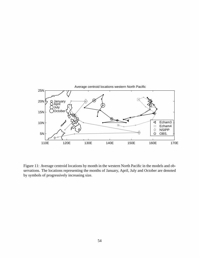
c. Tracks centroid

In some basins, such as the western North Pacific, the average model and observed centroid has a

well defined annual cycle (see Fig. 11). The average north latitude reaches its maximum in August,

and most equatorward position around February. Though the models’ biases in centroid longitude

are substantial, they reproduce the latitude-averaged annual cycle quite well.

If the interannual variability of the mean location of tropical cyclone activity is somewhat pre-

dictable, this could translate to predictability of year-to-year anomalies in landfall probabilities

for defined coastal regions. Interannual variability of mean latitude and longitude differs widely

among basins. In the Australian basin there is a much larger standard deviation for the mean lon-

gitude (6.7) than mean latitude (2.8), while in the the North Indian Ocean the standard deviations

of latitude and longitude are similar and small (2.6 and 2.9). Biases in the models’ climatological

centroid locations were discussed earlier. The models have a reasonable interannual variability

of the average latitude in the western North Pacific. In the Australian basin, NSIPP has a larger

interannual variability than the observations and the other two models, while the mean longitude

variability of the ECHAM4 model is too small. Further details on a basin-by-basin basis are avail-

28

able in Camargo et al. (2004a).

In tables 8 and 9 the correlations between the models and observations are shown for the cen-

troid latitude and longitude, respectively. Both ECHAM models have significant skill mainly for

the western North Pacific.

The tracks centroid location in the eastern North Pacific of ECHAM4 is very similar to that

observed, while ECHAM3 has a bias to the west and NSIPP to the east. Significant correlations

for centroid longitude also occur in this basin (Table 9). In the Atlantic, the centroid location of

ECHAM3 has an eastward bias while ECHAM4 and especially NSIPP have southwesterly biases.

Significant correlations for longitude appear in the North Indian Ocean.

In the South Pacific basin all models have high and significant skill for the centroid latitude.

Significant correlations are noted in the South Pacific, especially in the late season for all models

for the centroid longitude. The ECHAM4 model has significant skill for the centroid latitude in

the Australian basin.

5. Conclusions

Basic properties of tropical cyclones in three low-resolution AGCMs are examined. The AGCMs

were forced by observed SST, and produce ensembles of atmospheric responses. The two main

29

aims are to study the climatologies of model tropical cyclone behavior, and skill in simulating

observed interannual variability of aspects of tropical cyclone activity. Despite the low resolution,

the models demonstrated significant skill for some tropical cyclone properties on seasonal to annual

time-scales. Skills are model and basin dependent, and vary among tropical cyclone characteristics.

We cannot point to a single model as having the best skill across the different tropical cyclone

variables globally.

The tropical cyclone activity in all models occurs nearer the equator than in observations. All

models have low simulation skill in the Indian Ocean, both south and north of the equator. In the

North Indian Ocean even the tropical cyclone activity annual cycle is poorly simulated, likely due

to failure to reproduce the inhibiting effect of the summer monsoon and the consequent bimodal

observed annual cyclone cycle.3 For number of tropical cyclones (NTC), all models have signifi-

cant simulation skill in the South Pacific and the Atlantic. This may be due to a strong relationship

with ENSO in these two basins. The Atlantic and western North Pacific are the basins where the

models demonstrate significant skills for most variables. Lesser skill in the South Pacific for vari-

ables other than NTC may be due to relatively questionable data quality there, which would have

least impact on NTC.

Though the models’ tropical cyclones are considerably weaker than those observed, the mod-

3Proper simulation of the monsoon is difficult without using a fully coupled ocean-atmopshere model to reproduceatmosphere-to-ocean feedbacks known to play a key role in monsoon dynamics.

30

els’ MACE indices are significantly correlated with those observed in some basins. In the eastern

North Pacific, for instance, the ECHAM4 model does not have significant skill in the peak season

(JAS) for NTC, but has significant skill in that season for the MACE index.

Overall, ECHAM4 is the model with the most significant skill across the different properties,

especially in the western North Pacific and the South Pacific. ECHAM3 has generally better skill

in the Atlantic than the other models. NSIPP has very different characteristics in the Southern

versus Northern Hemispheres, being more similar to observations in the Southern Hemisphere.

Though NSIPP has a slightly higher numerical resolution than both ECHAM models, this does

not appear to translate to better simulated tropical cyclone activity characteristics, perhaps because

other factors are of equal importance, such as physical parametrization schemes (Vitart and Stock-

dale (2001)). For the cyclone genesis density pattern, the NSIPP model represents reality better

skill than the other two models.

The ECHAM3 and ECHAM4 models have very long tracks in the Southern Hemisphere com-

pared to the observations, and this is reflected in long cyclone lifetimes. Though the NSIPP model’s

tropical cyclones have shorter tracks in the Southern Hemisphere, the lifetimes are even longer, re-

flecting NSIPP’s very slow cyclone movement. The ECHAM3 and ECHAM4 models have some

skill in the interannual variability of the tropical cyclones’ lifetime in the western North Pacific,

but not in the other Northern Hemisphere basins.

31

An attempt was made to classify the models’ tropical cyclones into strength categories (trop-

ical storm, hurricane and intense hurricane). Skills within strength categories is low compared

with cyclone activity as a whole. Due to the low horizontal resolution of the models, their wind

speed distributions have much smaller positive skewness than the observed distribution. Although

bias corrections are made, the distinction among the strength categories involves the cyclones’

maximum speeds, which remain somewhat unrepresentative even after the correction.

In summary, some aspects of the observed tropical cyclone activity are reproduced by the

models fairly well, both in terms of model climatology and interannual variability. In some cases

biases in model climatology do not seriously preclude simulation skill for interannual variability, as

for instance in the Atlantic. Other aspects of cyclone behavior have significantly greater problems

and may still be handled most effectively by statistical tools at this point, such as tropical cyclone

numbers by strength category. Given the models’ low resolution, results shown here may be viewed

encouraging in the context of what might be possible using improved versions of these dynamical

tools. The relation between model tropical cyclone characteristics and ENSO is currently being

examined.

32

6. Acknowledgments

The authors thank Dr. Max Suarez and Michael Kistler (NSIPP) for making the NSIPP model

data available for this study, and Max-Planck Institute for Meteorology (Hamburg, Germany) for

making both versions of their model ECHAM accessible to IRI. We thank Dr. Simon Mason

for suggestions on statistical measures and comments on this paper, and Dr. Lisa Goddard for

discussions about our results. We thank Dr. M. Benno Blumenthal for the IRI data library and Drs.

Michael K. Tippett, Andrew W. Robertson and Adam Sobel for comments on this paper.

References

Arpe, K., L. Dumenil, and M. Giorgetta, 1998: Variability of the Indian Monsoon in the ECHAM3

Model: Sensitivity to Sea Surface Temperature, Soil Moisture and the Stratospheric Quasi-

Biennial Oscillation.J. Clim., 11, 1837–1858.

Avila, L., R. J. Pasch, J. L. Beven, J. L. Franklin, M. B. Lawrence, S. R. Stewart, and J. Jiing,

2003: Eastern North Pacific hurricane season of 2001.Mon. Wea. Rev., 131, 249–262.

Barnston, A. G., S. J. Mason, L. Goddard, D. G. DeWitt, and S. Zebiak, 2003: Multimodel ensem-

33

bling in seasonal climate forecasting at IRI.Bull. Amer. Meteor. Soc., 84, 1783–1796.

Bell, G. D., M. S. Halpert, R. C. Schnell, R. W. Higgins, J. Lawrimore, V. E. Kousky, R. Tinker,

W. Thiaw, M. Chelliah, and A. Artusa, 2000: Climate assessment for 1999.Bull. Amer. Meteor.

Soc., 81, S1–S50.

Bengtsson, L., 2001: Hurricane threats.Science, 293, 440–441.

Bengtsson, L., H. Bottger, and M. Kanamitsu, 1982: Simulation of hurricane-type vortices in a

general circulation model.Tellus, 34, 440–457.

Bengtsson, L., M. Botzet, and M. Esh, 1995: Hurricane-type vortices in a general circulation

model.Tellus, 47A, 175–196.

—, 1996: Will greenhouse gas-induced warming over the next 50 years lead to higher frequency

and greater intensity of hurricanes?Tellus, 48A, 57–73.

Broccoli, A. J. and S. Manabe, 1990: Can existing climate models be used to study anthropogenic

changes in tropical cyclone climate?Geophys. Rev. Lett., 17, 1917–1920.

Camargo, S. J., A. G. Barnston, and S. E. Zebiak, 2004a: Properties of tropical cyclones in atmo-

spheric general circulation models. IRI Technical Report 04-02, 72pp., International Research

Institute for Climate Prediction, Palisades, NY.

34

Camargo, S. J., H. Li, and L. Sun, 2002: Simulation of typhoons in the regional spectral model.

Abstracts of the 4th International RSM Workhsop, Los Alamos, NM, 7.

Camargo, S. J. and A. H. Sobel, 2004: Formation of tropical storms in an atmospheric general

circulation model.Tellus A, 56, 56–67.

Camargo, S. J. and S. E. Zebiak, 2002: Improving the detection and tracking of tropical storms in

Atmospheric General Circulation Models.Wea. Forecasting, 17, 1152–1162.

Chan, J. C. L., J. E. Shi, and C. M. Lam, 1998: Seasonal forecasting of tropical cyclone activity

over the Western North Pacific and the South China Sea.Wea. Forecasting, 13, 997–1004.

Cherchi, A. and A. Navarra, 2003: Reproducibility and predictability of the Asian summer mon-

soon in the ECHAM4-GCM.Clim. Dyn., 20, 365–379.

CPC, 2004: Available on line at http://www.cpc.noaa.gov/products/.

Franklin, J. L., L. A. Avila, J. L. Beven, M. B. Lawrence, R. J. Pasch, and S. R. Stewart, 2003:

Eastern North Pacific hurricane season of 2002.Mon. Wea. Rev., 131, 2379–2393.

Goddard, L., A. G. Barnston, and S. J. Mason, 2003: Evaluation of the IRI’s “Net Assessment”

seasonal climate forecasts: 1997-2001.Bull. Amer. Meteor. Soc., 84, 1761–1781.

Goddard, L., S. J. Mason, S. E. Zebiak, C. F. Ropelewski, R. E. Basher, and M. A. Cane, 2001:

35

Current approaches to seasonal to interannual climate predictions.Int. J. Climatol., 21, 1111–

1152.

Gray, W. M., C. W. Landsea, P. W. M. Jr., and K. J. Berry, 1993: Predicting Atlantic basin seasonal

tropical cyclone activity by 1 August.Wea. Forecasting, 8, 73–86.

—, 1994: Predicting Atlantic Basin Seasonal Tropical Cyclone Activity by 1 June.Wea. Forecast-

ing, 9, 103–115.

Haarsma, R. J., J. F. B. Mitchell, and C. A. Senior, 1993: Tropical disturbances in a GCM.Clim.

Dyn., 8, 247–257.

IRI, 2004: IRI (International Research Institute for Climate Prediction) Typhoon Activity Fore-

casts. available on line at: http://iri.columbia.edu/forecast/typhoon/.

JTWC, 2004: JTWC (Joint Typhoon Warning Center) best track dataset, available online at

https://metoc.npmoc.navy.mil/jtwc/besttracks/.

Krishnamurti, T. N., 1988: Some recent results on numerical weather prediction over the tropics.

Aust. Meteor. Mag., 36, 141–170.

Krishnamurti, T. N., D. Oosterhof, and N. Dignon, 1989: Hurricane prediction with a high resolu-

tion global model.Mon. Wea. Rev., 117, 631–669.

36

Lal, M., U. Cubash, J. Perliwitz, and J. Waszewitz, 1997: Simulation of the Indian monsoon

climatology in ECHAM3 climate model: sensitivity to horizontal resolution.Int. J. Clim., 17,

847–858.

Landman, W. A., A. Seth, and S. J. Camargo, 2002: The effect of regional climate model domain

choice on the simulation of tropical cyclone-like vortices in the southwestern Indian ocean.

IRI Technical Report 02-06, 31 pp., International Research Institute for Climate Prediction,

Palisades, NY, J. Climate, under revision (January, 2004).

Li, Z. X., 1999: Ensemble atmospheric gcm simulation of climate interannual variability from

1979 to 1994.J. Climate, 12, 986–1001.

Liu, K. S. and J. C. L. Chan, 2003: Climatological characteristics and seasonal forecasting of

tropical cyclones making landfall along the South China coast.Mon. Wea. Rev., 131, 1650–

1662.

Manabe, S., J. L. Holloway, and H. M. Stone, 1970: Tropical circulation in a time-integration of a

global model of the atmosphere.J. Atmos. Sci., 27, 580–613.

Mason, S. J., L. Goddard, N. E. Graham, E. Yulaeva, L. Q. Sun, and P. A. Arkin, 1999: The IRI

seasonal climate prediction system and the 1997/98 El Nino event.Bull. Amer. Meteor. Soc., 80,

1853–1873.

37

May, W. H., 2003: The Indian summer monsoon and its sensitivity to the mean SSTs: Simulations

with the ECHAM4 AGCM at T106 horizontal resolution.J. Meteor. Soc. Japan, 81, 57–83.

Model User Support Group, 1992: Echam3 - atmospheric general circulation model. Technical

Report 6, Das Deutshes Klimarechnenzentrum, Hamburg, Germany, 184pp.

Moorthi, S. and M. J. Suarez, 1992: Relaxed Arakawa-Schubert. a parameterization of moist con-

vection for general circulation models.Mon. Wea. Rev., 120, 978–1002.

NHC, 2004: NHC (National Hurricane Center) best track dataset, available online at

http://www.nhc.noaa.gov/pastall.shtml.

Peng, P. T., A. Kumar, A. G. Barnston, and L. Goddard, 2000: Simulation skills of the sst-forced

global climate variability of the ncep-mrf9 and the scripps-mpi echam3 models.J. Climate, 13,

3657–3679.

Roeckner, E., K. Arpe, L. Bengtsson, M. Christoph, M. Claussen, L. Dumenil, M. Esch, M. Gior-

getta, U. Schlese, and U. Schulzweida, 1996: The atmospheric general circulation model

ECHAM-4: Model description and simulation of present-day climate. Technical Report 218,

Max-Planck Institute for Meteorology, Hamburg, Germany, 90 pp.

Ryan, B. F., I. G. Watterson, and J. L. Evans, 1992: Tropical cyclone frequencies inferred from

38

Gray’s yearly genesis parameter: Validation of GCM tropical climate.Geophys. Res. Lett., 19,

1831–1834.

Sheskin, D. J., 2000:Handbook of Parametric and Nonparametric Statistical Procedures. Chap-

man & Hall/CRC, Boca Raton, Florida, USA, 2nd edition.

Suarez, M. J. and L. L. Takacs, 1995: Documentation of the Aries/GEOS dynamical core Version

2. NASA Technical Memorandum 104606, Vol 6., Goddard Space Flight Center, Greenbelt,

MD, 58 pp.

Sugi, M., A. Noda, and N. Sato, 2002: Influence of global warming on tropical cyclone climatol-

ogy: An experiment with the JMA global model.J. Meteor. Soc. Japan, 80, 249–272.

Thorncroft, C. and I. Pytharoulis, 2001: A dynamical approach to seasonal prediction of Atlantic

tropical cyclone activity.Wea. Forecasting, 16, 725–734.

Tiedtke, M., 1989: A comprehensive mass flux scheme for cumulus parametrization in large-scale

models.Mon. Wea. Rev., 117, 1779–1800.

TSR, 2004: Tropical Storm Risk, available online at http://tropicalstormrisk.com/.

Tsutsui, J. I. and A. Kasahara, 1996: Simulated tropical cyclones using the National Center for

Atmospheric Research community climate model.J. Geophys. Res., 101, 15013–15032.

39

Vitart, F., D. Anderson, and T. Stockdale, 2003: Seasonal forecasting of tropical cyclone landfall

over Mozambique.J. Climate, 16, 3932–3945.

Vitart, F., J. L. Anderson, and W. F. Stern, 1997: Simulation of interannual variability of tropical

storm frequency in an ensemble of GCM integrations.J. Climate, 10, 745–760.

—, 1999: Impact of large-scale circulation on tropical storm frequency, intensity and location,

simulated by an ensemble of GCM Integrations.J. Climate, 12, 3237–3254.

Vitart, F. D. and T. N. Stockdale, 2001: Seasonal forecasting of tropical storms using coupled

GCM integrations.Mon. Wea. Rev., 129, 2521–2537.

Walsh, K. and B. Ryan, 2000: Tropical cyclone intensity increase near australia as a result of

climate change.J. Climate, 13, 3029–3036.

Watterson, I. G., J. L. Evans, and B. F. Ryan, 1995: Seasonal and interannual variability of tropical

cyclogenesis: Diagnostics from large-scale fields.J. Climate, 8, 3052–3066.

Wu, G. and N. C. Lau, 1992: A GCM Simulation of the relationship between tropical storm

formation and ENSO.Mon. Wea. Rev., 120, 958–977.

40

List of Figures

1 Definition of the ocean basin domains used in this study: South Indian (SI),30 −

105E; Australian (AUS), (105E−165E); South Pacific (SP),165E−110W ; North

Indian (NI),45E − 100E; western North Pacific (WNP),100E − 160W , eastern

North Pacific (ENP),160W − 100W ; and Atlantic (ATL),100W − 0. All latitude

boundaries are along the equator and40◦N or 40◦S. Note the unique boundary

paralleling Central America for ENP and ATL basins. . . . . . . . . . . . . . . . . 44

2 Location of model tropical cyclone formation in one ensemble member of (a)

ECHAM3, (b) ECHAM4 and (c) NSIPP models, and in (d) observed names tropi-

cal cyclones. The period of coverage is 1961-2000. . . . . . . . . . . . . . . . . . 45

3 Mean number of tropical cyclone by formation position per year and ensemble

member per4◦ of (a) latitude (averaged over all longitudes), and (b) longitude (av-

eraged over all latitudes), for the models (ECHAM3 (dot-dashed line), ECHAM4

(dashed line), NSIPP (dotted line)), and observations (continuous line)) over the

period 1961-2000. . . . . . . . . . . . . . . . . . . . . . . . . . . . . . . . . . . . 46

41

4 Tracks of tropical cyclones for the years 1993-1995 for the one of the ensemble

members in the models: (a) ECHAM3, (b) ECHAM4 (c) NSIPP, and in the (d)

observations. . . . . . . . . . . . . . . . . . . . . . . . . . . . . . . . . . . . . . 47

5 Tropical cyclone track density per year for the models (per ensemble member)

(a) ECHAM3, (b) ECHAM4 (c) NSIPP, and for the observations (d) in the period

1961-2000. . . . . . . . . . . . . . . . . . . . . . . . . . . . . . . . . . . . . . . 48

6 (a) External (interannual), internal (inter-ensemble) and total standard deviation

(SD) in models and observations (total only) in the different basins. For each

basin, the first column is the SDs of ECHAM3, the second ECHAM4, the third

NSIPP and the fourth the observations. In bars showing model results, the shading

representing the smallest SD occupies the bar from zero up to its value. . . . . . . 49

7 Average number of tropical cyclones (NTC) per month in the models and observa-

tions in the period 1961-2000 in the Northern Hemisphere: (a) North Indian, (b)

western North Pacific, (c) eastern North Pacific, (d) North Atlantic. . . . . . . . . . 50

8 Time series showing the interannual variability of the number of tropical cyclones

(NTC) in the models and observations in the western North Pacific over the period

1961-2000. . . . . . . . . . . . . . . . . . . . . . . . . . . . . . . . . . . . . . . 51

42

9 Average MACE per month in the models and observations for (a) the Australian

basin, (b) South Indian Ocean, and (c) South Pacific (c). . . . . . . . . . . . . . . . 52

10 Time series of tropical cyclone activity (MACE) in the bias corrected models (en-

semble mean) and observations in the western North Pacific over the period 1961-

2000. . . . . . . . . . . . . . . . . . . . . . . . . . . . . . . . . . . . . . . . . . 53

11 Average centroid locations by month in the western North Pacific in the models

and observations. The locations representing the months of January, April, July

and October are denoted by symbols of progressively increasing size. . . . . . . . 54

43

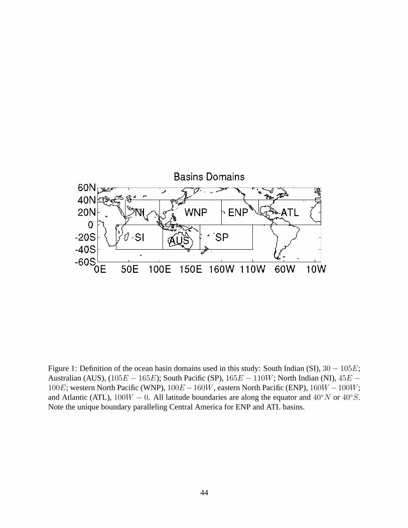
Figure 1: Definition of the ocean basin domains used in this study: South Indian (SI),30− 105E;Australian (AUS), (105E − 165E); South Pacific (SP),165E − 110W ; North Indian (NI),45E −100E; western North Pacific (WNP),100E−160W , eastern North Pacific (ENP),160W −100W ;and Atlantic (ATL),100W − 0. All latitude boundaries are along the equator and40◦N or 40◦S.Note the unique boundary paralleling Central America for ENP and ATL basins.

44

Figure 2: Location of model tropical cyclone formation in one ensemble member of (a) ECHAM3,(b) ECHAM4 and (c) NSIPP models, and in (d) observed names tropical cyclones. The period ofcoverage is 1961-2000.

45

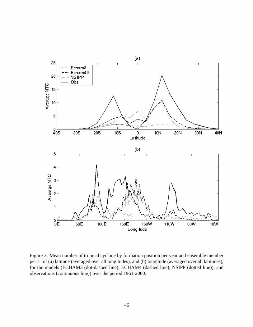
Figure 3: Mean number of tropical cyclone by formation position per year and ensemble memberper4◦ of (a) latitude (averaged over all longitudes), and (b) longitude (averaged over all latitudes),for the models (ECHAM3 (dot-dashed line), ECHAM4 (dashed line), NSIPP (dotted line)), andobservations (continuous line)) over the period 1961-2000.

46

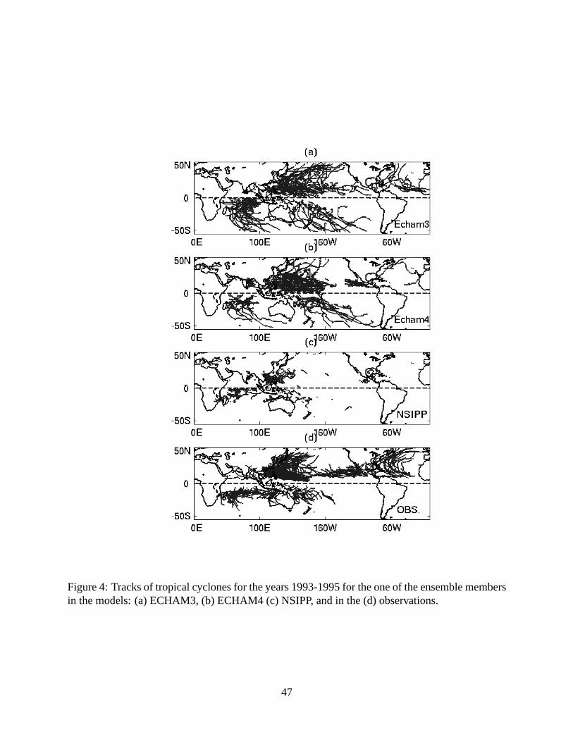
Figure 4: Tracks of tropical cyclones for the years 1993-1995 for the one of the ensemble membersin the models: (a) ECHAM3, (b) ECHAM4 (c) NSIPP, and in the (d) observations.

47

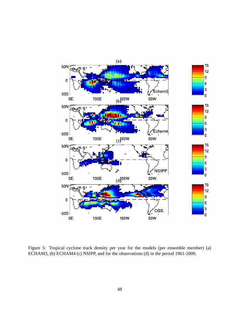
Figure 5: Tropical cyclone track density per year for the models (per ensemble member) (a)ECHAM3, (b) ECHAM4 (c) NSIPP, and for the observations (d) in the period 1961-2000.

48

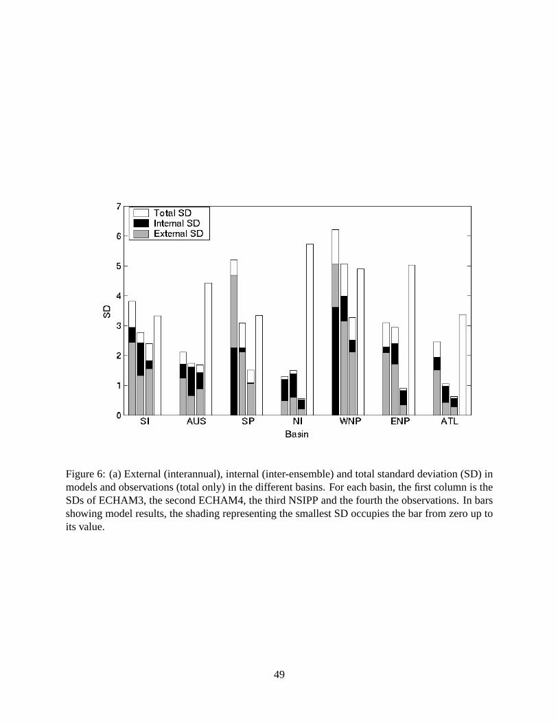
Figure 6: (a) External (interannual), internal (inter-ensemble) and total standard deviation (SD) inmodels and observations (total only) in the different basins. For each basin, the first column is theSDs of ECHAM3, the second ECHAM4, the third NSIPP and the fourth the observations. In barsshowing model results, the shading representing the smallest SD occupies the bar from zero up toits value.

49

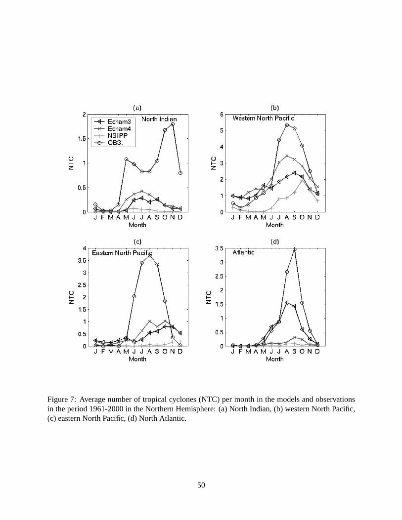
Figure 7: Average number of tropical cyclones (NTC) per month in the models and observationsin the period 1961-2000 in the Northern Hemisphere: (a) North Indian, (b) western North Pacific,(c) eastern North Pacific, (d) North Atlantic.

50

Figure 8: Time series showing the interannual variability of the number of tropical cyclones (NTC)in the models and observations in the western North Pacific over the period 1961-2000.

51

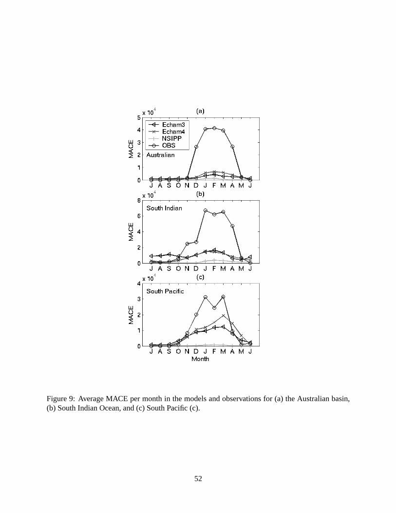
Figure 9: Average MACE per month in the models and observations for (a) the Australian basin,(b) South Indian Ocean, and (c) South Pacific (c).

52

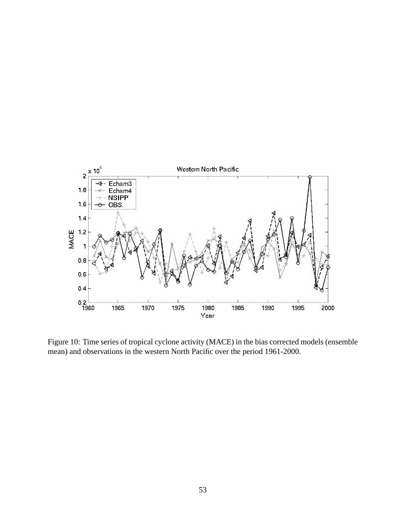
Figure 10: Time series of tropical cyclone activity (MACE) in the bias corrected models (ensemblemean) and observations in the western North Pacific over the period 1961-2000.

53

110E 120E 130E 140E 150E 160E 170E

5N

10N

15N

20N

25N

JanuaryAprilJulyOctober

Average centroid locations western North Pacific

Echam3Echam4NSIPPOBS.

Figure 11: Average centroid locations by month in the western North Pacific in the models and ob-servations. The locations representing the months of January, April, July and October are denotedby symbols of progressively increasing size.

54

List of Tables

1 Simulation properties and characteristics of the AGCMs. . . . . . . . . . . . . . . 58

2 Mean and standard deviation (SD) of NTC in all basins, northern (NH) and south-

ern (SH) hemispheres and globally (GL), with their respective percentage (Perc.)

contribution to the global totals in models and observations in the period 1961-2000 59

3 Correlations (Cor.) and mean square error (×10−2) (MSE) of track density per

year per ensemble member (Fig. 5) in models versus observations: globe (GL),

Northern Hemisphere (NH) and Southern Hemisphere (SH). Bold entries indicate

correlation values having significance at the95% confidence level. . . . . . . . . . 60

4 Mean, interannual standard deviation, and coefficient of variation of lifetime (in

days) of tropical cyclones in the globe (GL) , Northern Hemisphere (NH) and

Southern Hemisphere (SH) in models and observations in the period 1961-2000 . . 61

5 MACE mean (×104), standard deviation (SD) (×104) and coefficient of variation

(CV, or mean/SD) per year for all basins. . . . . . . . . . . . . . . . . . . . . . . . 62

55

6 Correlations between NTC in the models and observations, by basin, for relevant

seasons in the period 1971-2000. Only models and basins with at least one season

with significant correlation are shown. Bold entries indicate correlation values that

have significance at the95% confidence level. . . . . . . . . . . . . . . . . . . . . 63

7 Correlations of tropical cyclone activity (MACE) in the bias corrected models and

observations for relevant seasons. Period for western North Pacific, eastern North

Pacific and North Atlantic: 1971-2000; for North Indian, South Indian, Australian

and South Pacific: 1981-2000. Only models and basins with at least one season of

significant correlation are shown. Bold entries indicate correlation values having

significance at the90% confidence level. . . . . . . . . . . . . . . . . . . . . . . . 64

8 Correlations of the average latitude of tropical cyclone tracks in the models with

observations, by basin for different seasons in the period 1971-2000. Years with-

out tropical cyclones are omitted by model, season and basin. Only models and

basins with at least one season with significant correlation are shown. Bold entries

indicate correlation values having significance at the95% confidence level. . . . . 65

56

9 Correlations of the average longitude of tropical cyclone tracks in the models with

observations, by basin for different seasons in the period 1971-2000. Years with-

out tropical cyclones are omitted by model, season and basin. Only models and

basins with at least one season with significant correlation are shown. Bold entries

indicate correlation values having significance at the95% confidence level. . . . . 66

57

Model ECHAM3 ECHAM4 NSIPPPeriod 1961-2000 1961-2000 1961-2000

Ensemble Size 10 24 09Output Type six-hourly six-hourly dailyResolution T42 (spectral) T42 (spectral) 2.5◦ × 2◦ (grid point)

Convection Schememass flux - Tiedtke modified mass flux - Tiedtke relaxed Arakawa-Shubert

Table 1: Simulation properties and characteristics of the AGCMs.

58

Basin ECHAM3 ECHAM4 NSIPP OBS.Mean SD Perc. Mean SD Perc. Mean SD Perc. Mean SD Perc.

NI 1.3 0.5 2.7% 2.0 0.6 4.1% 0.3 0.2 1.9% 9.1 5.7 10.0%WNP 17.8 5.1 36.6% 23.9 3.1 49.5% 7.4 2.1 47.2% 27.4 4.9 30.1%ENP 4.2 2.1 8.6% 4.5 1.7 9.3% 0.3 0.2 1.9% 15.3 5.0 16.8%ATL 6.3 1.6 13.0% 2.2 0.6 4.6% 0.6 0.4 3.8% 10.0 3.4 11.0%NH 29.6 5.8 60.9% 32.6 3.6 67.5% 8.6 2.1 54.8% 61.8 8.4 67.9%SI 11.1 2.6 22.8% 6.7 1.4 13.9% 3.8 1.6 24.2% 12.9 3.9 14.2%

AUS 2.8 1.1 5.8% 3.1 0.7 6.4% 2.2 0.9 14.0% 10.5 4.0 11.5%SP 5.1 3.3 10.5% 5.9 1.6 12.2% 1.1 0.8 7.0% 5.8 3.2 6.3%SH 19.0 4.4 39.1% 15.7 1.8 32.5% 7.1 2.0 45.2% 29.2 5.8 32.1%GL 48.6 8.2 100% 48.3 3.3 100% 15.7 2.6 8.6% 91.0 10.3 61.8%

Table 2: Mean and standard deviation (SD) of NTC in all basins, northern (NH) and southern (SH)hemispheres and globally (GL), with their respective percentage (Perc.) contribution to the globaltotals in models and observations in the period 1961-2000

59

Model ECHAM3 ECHAM4 NSIPPCor. MSE Cor. MSE Cor. MSE

GL 0.55 2.8 0.66 3.0 0.52 3.0NH 0.56 4.5 0.64 5.2 0.51 5.0SH 0.59 3.2 0.70 2.8 0.58 3.0

Table 3: Correlations (Cor.) and mean square error (×10−2) (MSE) of track density per year perensemble member (Fig. 5) in models versus observations: globe (GL), Northern Hemisphere (NH)and Southern Hemisphere (SH). Bold entries indicate correlation values having significance at the95% confidence level.

60

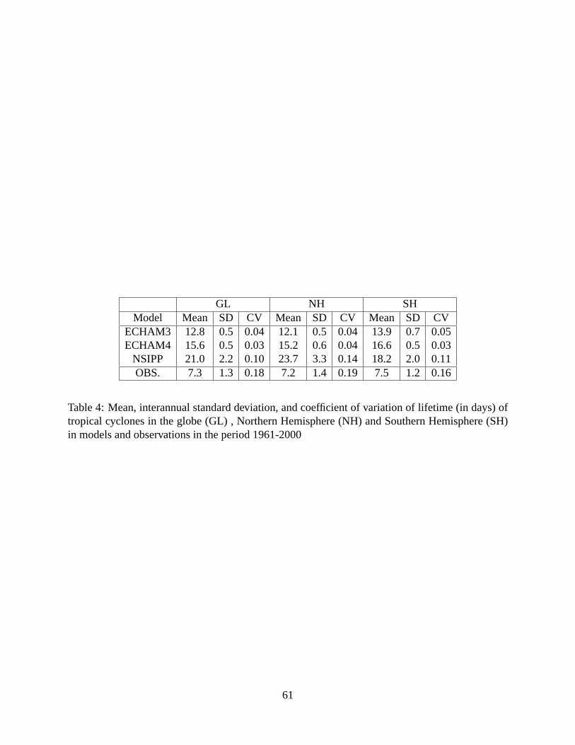
GL NH SHModel Mean SD CV Mean SD CV Mean SD CV

ECHAM3 12.8 0.5 0.04 12.1 0.5 0.04 13.9 0.7 0.05ECHAM4 15.6 0.5 0.03 15.2 0.6 0.04 16.6 0.5 0.03

NSIPP 21.0 2.2 0.10 23.7 3.3 0.14 18.2 2.0 0.11OBS. 7.3 1.3 0.18 7.2 1.4 0.19 7.5 1.2 0.16

Table 4: Mean, interannual standard deviation, and coefficient of variation of lifetime (in days) oftropical cyclones in the globe (GL) , Northern Hemisphere (NH) and Southern Hemisphere (SH)in models and observations in the period 1961-2000

61

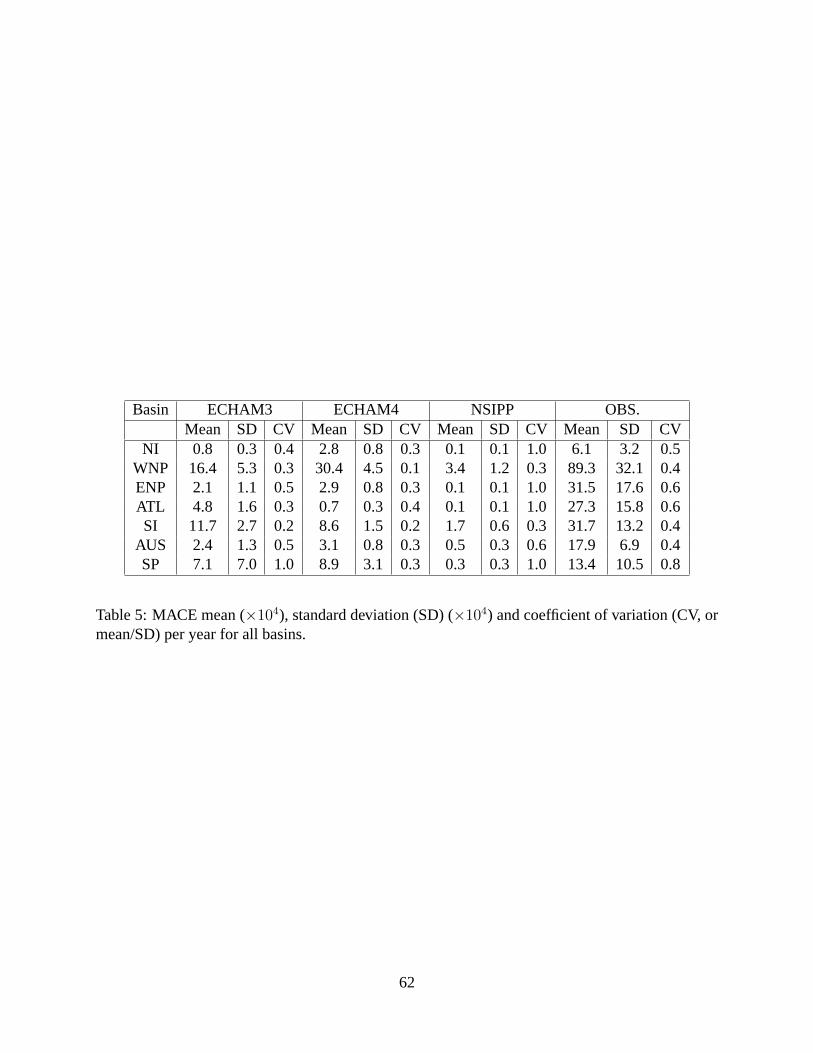
Basin ECHAM3 ECHAM4 NSIPP OBS.Mean SD CV Mean SD CV Mean SD CV Mean SD CV

NI 0.8 0.3 0.4 2.8 0.8 0.3 0.1 0.1 1.0 6.1 3.2 0.5WNP 16.4 5.3 0.3 30.4 4.5 0.1 3.4 1.2 0.3 89.3 32.1 0.4ENP 2.1 1.1 0.5 2.9 0.8 0.3 0.1 0.1 1.0 31.5 17.6 0.6ATL 4.8 1.6 0.3 0.7 0.3 0.4 0.1 0.1 1.0 27.3 15.8 0.6SI 11.7 2.7 0.2 8.6 1.5 0.2 1.7 0.6 0.3 31.7 13.2 0.4

AUS 2.4 1.3 0.5 3.1 0.8 0.3 0.5 0.3 0.6 17.9 6.9 0.4SP 7.1 7.0 1.0 8.9 3.1 0.3 0.3 0.3 1.0 13.4 10.5 0.8

Table 5: MACE mean (×104), standard deviation (SD) (×104) and coefficient of variation (CV, ormean/SD) per year for all basins.

62

Basin Model MJJ JJA JAS ASO SON OND JJASON Jan-DecWNP ECHAM3 0.37 0.29 0.24 0.33 0.20 0.10 0.36 0.40WNP ECHAM4 0.31 0.25 0.27 0.46 0.30 0.13 0.26 0.50ENP ECHAM4 0.47 0.42 0.33 0.39 0.29 0.10 0.42 0.40ATL ECHAM3 -0.04 0.39 0.56 0.33 0.12 0.02 0.53 0.55ATL ECHAM4 -0.10 0.28 0.43 0.42 0.29 0.20 0.52 0.52ATL NSIPP 0.22 0.52 0.38 0.31 0.06 0.14 0.38 0.45Basin Model NDJ DJF JFM FMA MAM AMJ NDJFMA Jul-Jun

SI ECHAM4 0.00 0.05 0.05 0.31 0.39 0.38 0.21 0.14AUS ECHAM4 0.02 0.34 0.43 0.51 0.35 0.24 0.41 0.38SP ECHAM3 0.64 0.49 0.44 0.52 0.50 0.39 0.72 0.73SP ECHAM4 0.53 0.42 0.31 0.39 0.31 0.24 0.52 0.60SP NSIPP 0.36 0.34 0.38 0.51 0.38 0.00 0.62 0.68

Table 6: Correlations between NTC in the models and observations, by basin, for relevant sea-sons in the period 1971-2000. Only models and basins with at least one season with significantcorrelation are shown. Bold entries indicate correlation values that have significance at the95%confidence level.

63

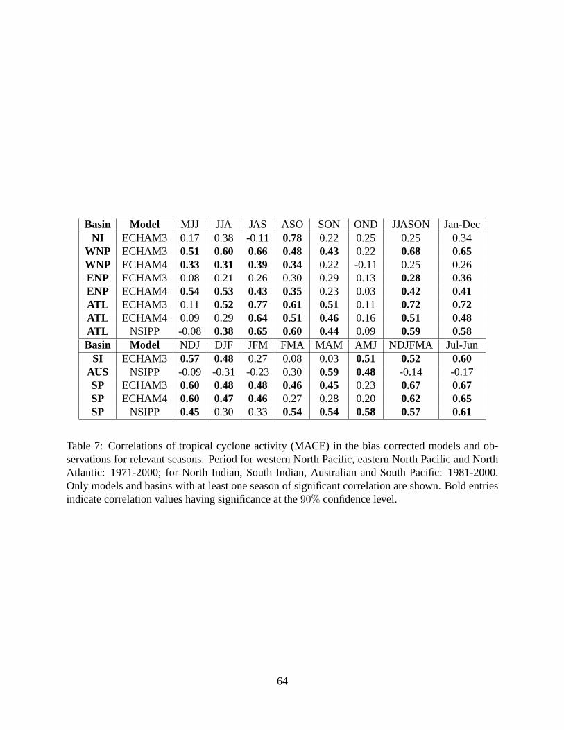
Basin Model MJJ JJA JAS ASO SON OND JJASON Jan-DecNI ECHAM3 0.17 0.38 -0.11 0.78 0.22 0.25 0.25 0.34

WNP ECHAM3 0.51 0.60 0.66 0.48 0.43 0.22 0.68 0.65WNP ECHAM4 0.33 0.31 0.39 0.34 0.22 -0.11 0.25 0.26ENP ECHAM3 0.08 0.21 0.26 0.30 0.29 0.13 0.28 0.36ENP ECHAM4 0.54 0.53 0.43 0.35 0.23 0.03 0.42 0.41ATL ECHAM3 0.11 0.52 0.77 0.61 0.51 0.11 0.72 0.72ATL ECHAM4 0.09 0.29 0.64 0.51 0.46 0.16 0.51 0.48ATL NSIPP -0.08 0.38 0.65 0.60 0.44 0.09 0.59 0.58Basin Model NDJ DJF JFM FMA MAM AMJ NDJFMA Jul-Jun

SI ECHAM3 0.57 0.48 0.27 0.08 0.03 0.51 0.52 0.60AUS NSIPP -0.09 -0.31 -0.23 0.30 0.59 0.48 -0.14 -0.17SP ECHAM3 0.60 0.48 0.48 0.46 0.45 0.23 0.67 0.67SP ECHAM4 0.60 0.47 0.46 0.27 0.28 0.20 0.62 0.65SP NSIPP 0.45 0.30 0.33 0.54 0.54 0.58 0.57 0.61

Table 7: Correlations of tropical cyclone activity (MACE) in the bias corrected models and ob-servations for relevant seasons. Period for western North Pacific, eastern North Pacific and NorthAtlantic: 1971-2000; for North Indian, South Indian, Australian and South Pacific: 1981-2000.Only models and basins with at least one season of significant correlation are shown. Bold entriesindicate correlation values having significance at the90% confidence level.

64

Basin Model MJJ JJA JAS ASO SON OND JJASON Jan-DecNI ECHAM4 -0.05 -0.06 -0.43 -0.24 0.16 0.51 -0.09 -0.08

WNP ECHAM3 0.21 0.61 0.56 0.39 0.07 0.10 0.36 0.54WNP ECHAM4 0.50 0.68 0.70 0.43 0.11 0.21 0.54 0.56ENP NSIPP 0.00 0.36 0.79 0.13 0.25 0.20 0.17 0.14Basin Model NDJ DJF JFM FMA MAM AMJ NDJFMA Jul-JunAUS ECHAM4 0.26 0.37 0.30 0.27 0.42 0.20 0.47 0.60SP ECHAM3 0.43 0.42 0.50 0.44 0.42 0.31 0.52 0.58SP ECHAM4 0.78 0.86 0.83 0.80 0.51 0.01 0.90 0.90SP NSIPP 0.50 0.66 0.70 0.64 -0.12 -0.33 0.72 0.65

Table 8: Correlations of the average latitude of tropical cyclone tracks in the models with obser-vations, by basin for different seasons in the period 1971-2000. Years without tropical cyclonesare omitted by model, season and basin. Only models and basins with at least one season withsignificant correlation are shown. Bold entries indicate correlation values having significance atthe95% confidence level.

65

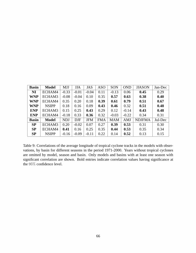
Basin Model MJJ JJA JAS ASO SON OND JJASON Jan-DecNI ECHAM4 -0.33 -0.01 -0.04 0.11 -0.13 0.06 0.45 0.29

WNP ECHAM3 -0.08 -0.04 0.10 0.35 0.57 0.63 0.38 0.40WNP ECHAM4 0.35 0.20 0.18 0.39 0.61 0.79 0.51 0.67WNP NSIPP 0.18 0.16 0.09 0.43 0.46 0.32 0.51 0.48ENP ECHAM3 0.15 0.25 0.43 0.29 0.12 -0.14 0.43 0.48ENP ECHAM4 -0.18 0.33 0.36 0.32 -0.03 -0.22 0.34 0.31Basin Model NDJ DJF JFM FMA MAM AMJ NDJFMA Jul-Dec

SP ECHAM3 0.20 -0.02 0.07 0.27 0.39 0.53 0.31 0.30SP ECHAM4 0.41 0.16 0.25 0.35 0.44 0.53 0.35 0.34SP NSIPP -0.16 -0.09 -0.11 0.22 0.14 0.52 0.13 0.15

Table 9: Correlations of the average longitude of tropical cyclone tracks in the models with obser-vations, by basin for different seasons in the period 1971-2000. Years without tropical cyclonesare omitted by model, season and basin. Only models and basins with at least one season withsignificant correlation are shown. Bold entries indicate correlation values having significance atthe95% confidence level.

66