Characteristics of inflation in Greece: Mean Spillover ...eprints.lse.ac.uk/32597/1/GreeSE_No43.pdf · Characteristics of inflation in Greece: ... the impact of oil price shocks on

All views expressed in this paper are those of the authors and do not necessarily represent the views of the Hellenic Observatory or the LSE

© Nicholas Apergis

Characteristics of inflation in Greece:

Mean Spillover Effects among CPI Components

Nicholas ApergisNicholas ApergisNicholas ApergisNicholas Apergis

GreeSE Paper No43GreeSE Paper No43GreeSE Paper No43GreeSE Paper No43

Hellenic Observatory Papers on Greece and Southeast EuropeHellenic Observatory Papers on Greece and Southeast EuropeHellenic Observatory Papers on Greece and Southeast EuropeHellenic Observatory Papers on Greece and Southeast Europe

January 2011January 2011January 2011January 2011

_

Table of Contents

ABSTRACTABSTRACTABSTRACTABSTRACT _______________________________________________________ iii

1. Introduction _______________________________________________________1

2. Inflation and the Economy of Greece ___________________________________5

3. Empirical Analysis _________________________________________________10

3.1. Data and Methodological Issues __________________________________10

3.2. Unit Roots Tests _______________________________________________11

3.3. Granger-Causality Tests and Price Transmissions ____________________13

3.4. Granger Causality Tests _________________________________________15

3.5. Variance Decompositions ________________________________________18

4. Discussion of the Results ____________________________________________24

5. Conclusions and Policy Implications __________________________________26

References _________________________________________________________28

AcknowledgementsAcknowledgementsAcknowledgementsAcknowledgements

The author wishes to thank an anonymous referee for providing valuable comments and suggestions that improved the quality of an earlier version of this paper. Needless to say, the usual disclaimer applies.

The Hellenic Observatory would like to thank the National Bank of Greece for its generous funding for this research.

Characteristics of inflation in Greece: Characteristics of inflation in Greece: Characteristics of inflation in Greece: Characteristics of inflation in Greece:

Mean Spillover Effects among CPI Components Mean Spillover Effects among CPI Components Mean Spillover Effects among CPI Components Mean Spillover Effects among CPI Components

Nicholas Apergis#

ABSTRACTABSTRACTABSTRACTABSTRACT

The objective of this paper is to investigate the behaviour of various

CPI components in terms of their spillover behaviour. This is the

first study analyzing the causal relationship between CPI

components in Greece. The empirical analysis uses data on different

components of the Consumer Price Index (CPI) with 1995 as the

base year (1995=100). Data covers the period 1981 to 2009. Our

results indicated the primary price movements are transmitted from

the energy price indices, i.e. the electricity price index, the energy

price index and the fuels and gas price index, while a secondary role

also comes from the food and vegetables price index along with the

services price index. In terms of causality, the evidence indicates

that there is a unidirectional transmission of energy prices

disturbance to the remaining CPI components, while innovations

(shocks) to the remaining CPI components did not have any

significant effect on all indices.

Keywords: CPI inflation, disaggregated data, spillover effects, VAR

models, Greece

# Nicholas Apergis, Department of Banking and Financial Management, University of Piraeus, Greece Correspondence: Nicholas Apergis, Department of Banking and Financial Management, University of Piraeus, 80 Karaoli & Dimitriou, 18534 Piraeus, Greece. Tel. 0030-2104142429, Fax: 0030-2104142341, E-mail: [email protected]

ChChChCharacteristics of inflation in Greece: aracteristics of inflation in Greece: aracteristics of inflation in Greece: aracteristics of inflation in Greece:

Mean Spillover Effects among CPI ComponentsMean Spillover Effects among CPI ComponentsMean Spillover Effects among CPI ComponentsMean Spillover Effects among CPI Components

1. Introduction

The reaction of consumer prices and inflation to fuel price movements has been

investigated by many authors, such as Hooker (2002), Barsky and Kilian

(2004) and LeBlanc and Chinn (2004). While Barsky and Kilian (2004) argue

that fuel prices increases generate strong inflationary shocks, LeBlanc and

Chinn (2004) argue that fuel prices have only a moderate effect on inflation.

Moreover, Ferderer (1996) argues that inflation has a negative impact on

investment, through a rise in firms’ costs and higher uncertainty, leading to

postponement of investment decisions and, thus, to lower production and,

through conditions of excess demand, to further higher prices. Van Den Noord

and Andre (2007), however, provide evidence that the fact the knock-on effects

from energy shocks onto core inflation appear weaker versus their counterparts

in the 1970s, a fact attributed to the fall in energy intensity as well as to a

persistent slack in the aftermath of the bursting of the dotcom bubble.

Moreover, the literature argues that oil price shocks can partially pass through

into inflation. The link between the two variables is highly important,

2

especially from the front of monetary economic policy implementation, since

monetary authorities attempt to keep inflation under control. In empirical

terms, the statistical relationship between oil price shocks and the real

economy, including the dynamics of inflation, has been estimated by a series of

studies. In particular, Blanchard and Gali (2007) with data from the G7

economies provide evidence that suggests that a number of factors determine

the impact of oil price shocks on inflation, such as the smaller share of oil in

production, the higher flexibility in labour markets and improvements in

monetary policy. Gregorio et al. (2007) display a substantial decline in oil pass-

through, while Den Noord and Andre (2007) also provide evidence that the

spillover effects of energy prices into core inflation are small to their

counterparts in the 1970s. All these studies explain this diminishing influence

of oil shocks through the fall in energy intensity. By contrast, Chen (2009)

claim that this energy intensity varies across countries and is positively

correlated with energy imports. The intensity depends on certain factors, such

as the appreciation of domestic currencies and the higher degree of trade

openness.

The use of highly aggregated data for causal inference is quite common in the

applied econometric literature. On one side there are researchers who use

Granger causality tests with mostly quarterly or annual data (Jung and

Marshall, 1985; Rao 1989; Demitriades and Hussein 1996). On the other side

are those who use cross-country regressions with data averaged over many

3

years. Causality in these studies is pre-imposed and testing is done on the

contemporaneous correlations (Grier and Tullock, 1989; Barro, 1991; Levine

and Renelt, 1992; King and Levine, 1993; Levine and Zervos, 1993; Frankel

and Roamer, 1999). A number of the above studies have focused on

aggregation and the dynamic relationships between variables and shown that

aggregation weakens the distributed lag relationships. In addition, they find that

aggregation turns one-way causality into a feedback system, while it produces

inconsistent estimates and induces endogeneity into previously exogenous

variables. Although these studies have already pointed out some potential

problems associated with aggregated data, a comprehensive study that focuses

on Granger causality with disaggregated data would be of immense value

because of the practical significance of causality testing based on aggregated

data. Finally, Gulasekaran and Abeysinghe (2002) and Gulasekaran (2004)

have derived quantitative results using an analytical framework to assess the

nature of the problems created. Overall, the following conclusions emerge.

Within a stationary framework, aggregation may (i) create a spurious feedback

loop from a unidirectional relation, (ii) erase a feedback loop and create a

unidirectional relation and (iii) erase the Granger-causal link altogether. The

distortions magnify when differencing is used after aggregation to induce

stationarity.

In Greece, some components of the price index exhibit a differentiated

behaviour and the relationship with disaggregated price indices may differ

4

among them. It is also clear that it is hard to predict the part of inflation that is

not related to domestic economic variables. For instance, fuel prices, which are

an important cause of inflation, cannot be predicted with an acceptable degree

of accuracy. Because of these reasons we also look at this problem on a

disaggregated basis. Hence, our main research question is: ‘What is the nature

of the causality between price inflation indices?’ Our secondary research

question is: ‘Are disaggregated data more informative about inflationary

developments than the main macroeconomic variables?’

This study aims at estimating the nature of the links between the

abovementioned variables. As a result, since inflation is a painful problem, we

would like to give our contribution to investigating and forming the economic

rationale behind the policy decisions affecting prices in the Greek economy.

Therefore, the objective as well as the novelty of this paper is to investigate the

behaviour of various CPI components in terms of their spillover behaviour. It is

expected that certain CPI components would have not been so responsive to

changes in other CPI components.

This is believed to be the first study analyzing the causal relationship between

CPI components in Greece. Our analysis thus encloses the information from all

available sectors of the price index. The research on commodities prices

spillover effects has focused exclusively on the international transmission of

such indexes movements. This paper, in contrast, tests whether movements in

CPI components initially affect one another.

5

Among the time series approaches univariate measures are distinguished from

multivariate methods. The univariate measures differ with respect to the

smoothing techniques that are applied. Simple methods like taking moving

averages. The multivariate methods basically comprise the vector

autoregression (VAR) approach suggested to the measurement of any type of

inflation by Quah and Vahey (1995).

2. Inflation and the Economy of Greece

Entry into the Eurozone provided Greece with an improved, stability-oriented

environment. The establishment of the euro as the single currency constitutes a

big step towards European integration. The European Central Bank was the

guardian of monetary stability, while the Stability and Growth Pact was

supposed to help ensure fiscal discipline. These changes were crucial benefits

for a country carrying the experience of high inflation rates (being at double-

digit levels from the early 80s to the mid 90s). In particular, inflation rates were

reduced from above 5% in late 1990’s to 1.2% in 2009, though the trend has

been upward again, due to unfavourable effects, such as higher oil and food

prices and higher domestic consumption taxes.

Although inflation in the Eurozone era was low by the country’s historical

standards, inflation was relatively high by euro-area standards. The differential

with the euro area still remained high (Figure 1). This was due not only to the

6

so-called Balassa-Samuelson Effect (Apergis, 2010), but also to other factors,

such as structural characteristics of the economy linked to the malfunctioning

of domestic markets (labour market rigidities, i.e. long-term unemployment,

low average job tenure, low gross labour flows between industries and sectors,

wage-setting institutions, i.e. wage bargaining is highly centralised, wages

increases in the public sector well above productivity growth, and

imperfections in the functioning of product markets and the reduced degree of

competition in many sectors, leading to fast-growing mark-ups), the persistent

falling of national savings (primarily due to the presence of persistent public

deficits, Figure 2) and the impact of energy costs on the performance of the

majority of sectors in the economy (ECB, 2005).

Figure 1. Greek inflation and inflation differential with EU.

Source: ECB (2005)

7

Figure 2. General government deficit (% GDP)

Source: Ministry of Economy: Greece Notes: SGP shows the projected fiscal deficit under the new stability programme, while the EC shows the projected fiscal deficit prepared of the Greek Ministry of Economy in cooperation with European Committee research analysts.

Moreover, being a member of the Eurozone brought cheap loans and large

inflows of capital. But those capital inflows also led to inflation. Wage

increases, adjusted for productivity changes, also were much higher than

average increase in the other Eurozone member economies. Thus, the rapid rise

of wage costs and mark-ups in excess of productivity growth, has contributed

to a wage-price spiral. With both prices and wages growing at high rates,

competitiveness declined. Over the period 2001-2009, competitiveness, as

measured by consumer prices, declined by 20 per cent, measured by unit labour

8

costs, declined by 25 per cent. As a result, the current account deficit rose to

about 14 per cent of GDP by the end of 2008.

As a result, along with the painful process of fiscal consolidation, the country

needs a substantial ‘internal devaluation’, e.g. a decline in prices to restore

competitiveness and rebalance the economy towards external demand, though

the largest sector of the economy, i.e. the services sector, does not show any

signals of competitiveness deterioration, while agricultural products, durables

and semi-durables have witnessed the sharpest lost in competitiveness. The

reason is the absence of any incentive in those sectors to increase productivity.

Therefore, policy makers must address the overall competitiveness

deterioration via structural reforms in product markets, which will weaken the

pricing power of oligopolies and enhance price competitiveness.

Figure 3 displays relative prices of the three main sectors of tradable goods and

services against major trading partners. The picture shows that prices for

industrial and agricultural products have increased about 30% relative to the

twelve major trading partners since 2000. By contrast, relative prices in the

services sector (measured against the 6 major competitors in tourist services)

have remained relatively stable, suggesting that price competitiveness in this

sector has not deteriorated over the last decade.

9

Figure 3. Prices relative to major trading partners

Source: Bank of Greece, 2010 Governor’s Annual Report Notes: BoG = Bank of Greece, Eurobank – estimates by the research analysis department of the Eurobank, Greece.

Nevertheless, a reasonably high rate of inflation will have the positive side

effect of making the reversal of the debt-to-GDP ratio easier than it is expected.

Hence, of the ECB is forced to maintain a more expansionary stance in

monetary policy to balance out the effects of painful fiscal consolidation,

inflation might increase.

10

3. Empirical Analysis

3.1. Data and Methodological Issues

The empirical analysis uses data on different components of the Consumer

Price Index (CPI) with 1995 as the base year (1995=100). Data covers the

period 1981 to 2009. The index is Laspeyres chained. Data comes from the

Datastream database and is based on a quarterly basis. Finally, we employ the

RATS 6.1 software to serve the goals of our empirical analysis.

The short-run dynamic interactions among the variables are characterized by

feedbacks going from one variable to the other or in both directions, depending

on the causal relationship. This provides justification for examining the

direction of the causal links among the variables under consideration through

Granger causality tests.

Several time-series methods have been developed to study interrelationships

among various variables, including commodities price indices. Vector

Autoregression (VAR) models have extensively been used to study the

contemporaneous correlations among various indices and to examine the

dynamic response of certain markets to artificial shocks. We use a VAR model

to study the interrelationships between the various components of the CPI

index in Greece. The VAR model allows us to capture both the

contemporaneous and lagged influence of the endogenous variables on each

other. It is also well suited to study dynamic responses of the variables to

11

shocks by way of the variance decomposition (VDCs) analysis. Another

important property of VAR models is that it is not restrictive if error terms are

serially correlated, because any serial correlation can be removed by adding

more lags to the dependent variables.

To serve better our research goal and to overcome certain statistical

deficiencies due to the lack of adequate observations, we aggregate (as a

weighted average) certain CPI components. In particular, the following

categories of CPI will be used in the analysis: Electricity (EL), Energy (EN),

Fuels and gas (FG), Food and vegetables (FV), Services (SER), Beverages

(BEV), Durables (DUR), Education (ED), Health (H) and Semi-durables

(including clothing, footwear and furniture) (SDUR). Throughout the empirical

analysis, lower case letters indicate variables in logarithms.

3.2. Unit Roots Tests

The results related to unit root tests are reported in Table 1. The ADF test is

based on the following regression model, assuming a drift and linear time

trend:

p

∆yt = a0 + Σ∆yt−1 + β t + γ yt-1 + εt

i=1

12

where t = time trend and εt = random error. The null hypothesis in the ADF test

is that there is a unit root where γ = 0. For all the variables to be stationary, we

must reject the null hypothesis in favour of the alternative hypothesis.

As suggested by Enders (1995), we carried out unit root tests on the

endogenous variables. Table 1 reports that based on augmented Dickey-Fuller

[1981] tests, the hypothesis that the variables el, en, fg, fv, ser, bev, dur, ed, h

and sdur contain a unit root cannot be rejected at the 5 percent significant level.

When first differences are used, unit root nonstationarity is rejected at the 5

percent significant level, suggesting that all the variables under study are I(1)

variables.

Table 1. Augmented Dickey-Fuller unit-root tests

Without Trend With Trend

Variables Levels First

Differences Levels

First Differences

el -0.88(4) -4.11(3)* -0.99(3) -4.36(2)*

en -0.71(5) -5.63(3)* -1.74(3) -7.14(2)*

fg -0.34(4) -4.71(3)* -1.77(4) -6.08(3)*

fv -1.05(3) -4.48(2)* -1.93(4) -5.11(2)*

ser -1.54(3) -4.56(2)* -1.37(4) -6.03(2)*

bev -2.53(4) -4.47(3)* -2.84(4) -4.93(2)*

dur -1.78(4) -4.84(3)* -1.94(3) -5.12(2)*

ed -1.63(4) -4.56(2)* -1.85(4) -4.88(2)*

h -1.77(4) -4.38(3)* -2.10(4) -4.69(3)*

sdur -1.68(3) -4.71(2)* -1.90(4) -4.93(3)*

Note: Figures in brackets denote the number of lags in the augmented term that ensures white-noise residuals. *denotes significance at the 5 percent level.

13

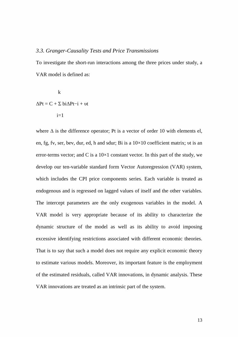
3.3. Granger-Causality Tests and Price Transmissions

To investigate the short-run interactions among the three prices under study, a

VAR model is defined as:

k

∆Pt = C + Σ bi∆Pt−i + υt

i=1

where ∆ is the difference operator; Pt is a vector of order 10 with elements el,

en, fg, fv, ser, bev, dur, ed, h and sdur; Bi is a 10×10 coefficient matrix; υt is an

error-terms vector; and C is a 10×1 constant vector. In this part of the study, we

develop our ten-variable standard form Vector Autoregression (VAR) system,

which includes the CPI price components series. Each variable is treated as

endogenous and is regressed on lagged values of itself and the other variables.

The intercept parameters are the only exogenous variables in the model. A

VAR model is very appropriate because of its ability to characterize the

dynamic structure of the model as well as its ability to avoid imposing

excessive identifying restrictions associated with different economic theories.

That is to say that such a model does not require any explicit economic theory

to estimate various models. Moreover, its important feature is the employment

of the estimated residuals, called VAR innovations, in dynamic analysis. These

VAR innovations are treated as an intrinsic part of the system.

14

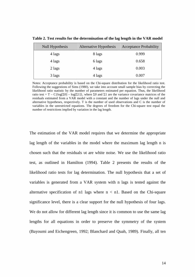
Table 2. Test results for the determination of the lag length in the VAR model

Null Hypothesis Alternative Hypothesis Acceptance Probability

4 lags 8 lags 0.999

4 lags 6 lags 0.658

2 lags 4 lags 0.003

3 lags 4 lags 0.007

Notes: Acceptance probability is based on the Chi-square distribution for the likelihood ratio test. Following the suggestions of Sims (1980), we take into account small sample bias by correcting the likelihood ratio statistic by the number of parameters estimated per equation. Thus, the likelihood ratio test = T – C{log[Σ0] – log[Σ1]}, where Σ0 and Σ1 are the variance covariance matrices of the residuals estimated from a VAR model with a constant and the number of lags under the null and alternative hypotheses, respectively. T is the number of used observations and C is the number of variables in the unrestricted equations. The degrees of freedom for the Chi-square test equal the number of restrictions implied by variation in the lag length.

The estimation of the VAR model requires that we determine the appropriate

lag length of the variables in the model where the maximum lag length n is

chosen such that the residuals υt are white noise. We use the likelihood ratio

test, as outlined in Hamilton (1994). Table 2 presents the results of the

likelihood ratio tests for lag determination. The null hypothesis that a set of

variables is generated from a VAR system with n lags is tested against the

alternative specification of n1 lags where n < n1. Based on the Chi-square

significance level, there is a clear support for the null hypothesis of four lags.

We do not allow for different lag length since it is common to use the same lag

lengths for all equations in order to preserve the symmetry of the system

(Bayoumi and Eichengreen, 1992; Blanchard and Quah, 1989). Finally, all ten

15

equations include a dummy variable that considers the 1992 EMU event. This

variable takes values of one for the last quarter in 1992 and zero otherwise.

3.4. Granger Causality Tests

Granger-causality is examined through Wald tests for block exogeneity, which

allows us to examine whether the lag structure of an excluded variable adds to

the explanatory power of the estimated equation. In other words, a test of

causality is whether the lags of one variable enter the equation for another

variable. Table 3 presents the most important Granger-causality test results. All

equations support certain econometric diagnostics, such as absence of serial

correlation (LM), absence of misspecification (RESET) and presence of

homoskedasticity (HE).

In particular, electricity prices (el), energy prices (en) and fuel and gas prices

(fg) Granger-cause all the remaining seven CPI components. Next, services

prices (ser), education prices (ed) and health prices (h) Granger cause durables

prices (dur) and semi-durables prices (sdur). Finally, Food and vegetables

prices (fv) Granger cause education prices (ed) and health prices (h). The

results do not support the presence of significant feedbacks between aggregate

CPI components.

16

Table 3. Granger causality tests

Equation Null Hypothesis Wald-

Statistic p-value

∆fv Electricity prices do not cause food and vegetables prices 22.35 0.00

LM = 6.54[0.52] RESET = 1.63[0.27] HE = 1.83[0.37]

∆ser Electricity prices do not cause services prices 29.06 0.00

LM = 10.72[0.41] RESET = 1.42[0.34] HE = 0.81[0.49]

∆bev Electricity prices do not cause beverages and beer prices 21.36 0.00

LM = 16.33[0.27] RESET = 1.46[0.32] HE = 0.70[0.53]

∆dur Electricity prices do not cause durables prices 19.55 0.00

LM = 14.35[0.32] RESET = 1.49[0.31] HE = 0.93[0.47]

∆ed Electricity prices do not cause education prices 35.82 0.00

LM = 13.27[0.37] RESET = 1.11[0.39] HE = 0.71[0.54]

∆h Electricity prices do not cause health prices 31.06 0.00

LM = 10.09[0.46] RESET = 1.16[0.44] HE = 0.49[0.69]

∆sdur Electricity prices do not cause semi-durables prices 21.28 0.00

LM = 5.43[0.67] RESET = 1.28[0.42] HE = 0.52[0.64]

∆fv Energy prices do not cause food and vegetables prices 24.71 0.00

LM = 15.49[0.37] RESET = 2.44[0.22] HE = 0.81[0.42]

∆ser Energy prices do not cause services prices 17.11 0.00

LM = 13.29[0.43] RESET = 2.36[0.20] HE = 0.39[0.71]

∆bev Energy prices do not cause beverages and beer prices 25.46 0.00

LM = 17.40[0.27] RESET = 2.08[0.25] HE = 1.12[0.31]

∆dur Energy prices do not cause durables prices 18.89 0.00

LM = 16.44[0.30] RESET = 1.96[0.23] HE = 0.73[0.38]

∆ed Energy prices do not cause education prices 39.76 0.00

LM = 3.58[0.81] RESET = 1.09[0.56] HE = 0.62[0.41]

∆h Energy prices do not cause health prices 28.93 0.00

LM = 14.42[0.26] RESET = 2.11[0.28] HE = 0.67[0.38]

∆sdur Energy prices do not cause semi-durables prices 23.28 0.00

LM = 11.07[0.33] RESET = 2.48[0.16] HE = 0.56[0.43]

17

Equation Null Hypothesis Wald-

Statistic p-value

∆fv Fuel prices do not cause food and vegetables prices 27.15 0.00

LM = 10.51[0.57] RESET = 1.36[0.24] HE = 0.72[0.39]

∆ser Fuel prices do not cause services prices 18.88 0.00

LM = 9.37[0.68] RESET = 1.18[0.29] HE = 1.88[0.16]

∆bev Fuel prices do not cause beverages and beer prices 18.35 0.00

LM = 11.62[0.51] RESET = 1.72[0.21] HE = 0.52[0.42]

∆dur Fuel prices do not cause durables prices 17.24 0.00

LM = 12.35[0.48] RESET = 1.67[0.23] HE = 0.66[0.35]

∆ed Fuel prices do not cause education prices 26.72 0.00

LM = 8.54[0.72] RESET = 1.19[0.18] HE = 0.62[0.45]

∆h Fuel prices do not cause health prices 26.33 0.00

LM = 9.11[0.53] RESET = 1.64[0.20] HE = 0.83[0.34]

∆sdur Fuel prices do not cause semi-durables prices 29.09 0.00

LM = 14.83[0.38] RESET = 2.06[0.13] HE = 0.62[0.44]

∆dur Services prices do not cause durables prices 37.19 0.00

LM = 13.72[0.50] RESET = 1.44[0.21] HE = 0.82[0.34]

∆sdur Services prices do not cause semi-durables prices 28.84 0.00

LM = 14.52[0.46] RESET = 1.72[0.19] HE = 0.75[0.35]

∆dur Education prices do not cause durables prices 34.48 0.00

LM = 7.38[0.68] RESET = 2.10[0.17] HE = 1.05[0.30]

∆sdur Education prices do not cause semi-durables prices 37.49 0.00

LM = 9.84[0.58] RESET = 1.81[0.20] HE = 0.82[0.34]

∆dur Health prices do not cause durables prices 36.82 0.00

LM = 17.48[0.28] RESET = 2.13[0.18] HE = 0.55[0.51]

∆sdur Health prices do not cause semi-durables prices 24.49 0.00

LM = 13.34[0.33] RESET = 1.66[0.24] HE = 0.84[0.40]

∆ed Food and vegetables prices do not cause durables prices 41.01 0.00

LM = 11.92[0.46] RESET = 2.16[0.16] HE = 0.52[0.50]

∆h Food&vegetables prices do not cause semi-durables prices 34.58 0.00

LM = 11.32[0.47] RESET = 1.18[0.42] HE = 0.67[0.45]

18

3.5. Variance Decompositions

To ascertain the importance of the dynamic relationship among the variables

under study, we obtained forecast error variance decompositions. Variance

decompositions tell us the percentage of the variance in a variable that is due to

its own “shock” and the “shocks” of the other variables in the VAR system. If a

shock explains none of the forecast error variance of a particular variable at all

forecast periods, it means that this particular variable evolves independently of

the series. In other words, this variable sequence is exogenous. On the other

extreme, the variable would be endogenous if all of its error variance is

explained by the shock. This analysis allows us to examine the relative

importance of each random innovation to the variables in the VAR system. In

standard VAR methodology the contemporaneous correlation among the

variables involved in the system is purged by the Cholesky orthogonalization

procedure.

Tables 4 through 10 capture the variance decompositions and the results

indicate that each series explains a substantial proportion of its own past values.

It is also interesting to note that as the time horizon expands, a particular

variable accounts for smaller proportions of its forecast error variance. The

followed results correspond to the following ordering of equations: fv, el, en,

fg, ser, bev, dur, ed, h, sdur. Generally speaking, this ordering reflects the fact

that fuel prices have an influence on all the remaining variables in their model,

19

but their own behaviour is least determined by other variables included in the

model. This is quite a plausible assumption, because fuel prices are largely

determined by world market conditions, rather than conditions within the Greek

economy (although, tax policy may put extra burden to those who make use of

fuel prices as well as to the rest of the economy, through the indirect channel of

the cost of production).

Table 4. Variance decompositions of food and vegetables price index (fv-%)

Period fv el en fg ser bev dur ed h sdur

1 41.1 16.2 10.3 9.0. 5.2 3.2 4.4 1.4 5.2 4

4 35.6 20.4 19.3 10.6 6.9 2.9 2.6 2.3 4.7 1

8 30.3 22.8 20.5 12.1 6.9 4.7 5.1 3.7 6.1 2

12 24.9 25.3 26.2 18.7 7.1 5.7 5.6 4.9 9.4 1

Notes: Numbers represent the percentage of the variance of the nth-period ahead forecast error for prices that are explained by the variables in the VAR model.

Table 4 indicates that the variance in the food and vegetables index could be

explained mainly by itself and developments in the electricity, energy and fuels

and gas indices. Over a 20 quarter time period, between 35% and 40% of the

forecast error variance in this index could be traced to the shocks in the three

indices mentioned above. In the first quarter following the shock, the food and

vegetables index explains about 41% of its own variance, while 16%, 10% and

9% is explained by the electricity, energy and fuels and gas indices,

respectively. Only after the fourth quarter do we observe a significant portion

20

of the food and vegetables index variance that is explained more heavily by the

remaining price indices.

Table 5. Variance decompositions of services price index (ser-%)


1 4.5 15.7 10 8.0. 35.3 2.5 6.4 4.4 2.2 11

4 4.7 19.4 12.9 9.2 29.5 2.5 5.8 4.5 2.5 9

8 5.6 21.4 15.3 10.2 22.5 3.9 6.2 4.8 4.1 6

12 6.2 24.2 18 13.3 17.4 4.1 6.1 4.8 4.9 4

Notes: Similar to Table 4

Table 5 shows the variance decompositions of the services price index. It

indicates that in the very short-run the services index is mainly explained by the

electricity price index (16%), the energy price index (10%), the semi-durable

price index (11%) and the fuel and gas price index (8%). All these four price

indices explain a relatively significant proportion of the services price index

forecast error variance. Their portion remains at high levels even after 20

quarters. The results suggest that there is a significant spillover effect between

services prices and energy prices. This seems to support our premise that the

services sector movements are significantly affected by the developments and

the cost structure in the energy sector even in the long-run.

21

Table 6. Variance decompositions of beverages and beer price index (bev-%)


1 5 17.3 11.1 10.0. 4.1 32 3.4 3.2 7.2 6.7

4 5.2 19 12.5 11.4 4.5 23.6 3.9 3.8 7.6 8.5

8 5 22.5 14.2 13.6 5.2 19.3 4.3 4.2 7.7 4

12 4.8 24.1 16.7 14.7 5.9 12.5 5 4.6 8.3 3.4


Table 6 summarizes the forecast error decomposition of the beverages and beer

price index. It seems that this index’s movements are explained by a sizeable

proportion of the three price indices related to the energy sector error variance

both in the short- and in the long-run. This is an interesting finding as we

expected that one more industrial sector’s cost movements in Greece would be

affected by energy sector’s developments.

Table 7. Variance decompositions of durables price index (dur-%)


1 5.1 15.3 10.5 12.4. 18.1 2.3 25.3 4.3 7.7 1

4 5.2 17.1 11 13.8 18.2 2.6 20.2 4.5 7.4 0

8 5.4 19.5 12.4 15.2 18.2 2.3 14.7 4.1 7.1 1.2

12 5.6 20.1 13.4 17.1 18.9 2.5 10.5 4 7.2 0.7


Table 7 shows the variance decompositions of the durables price index. It

indicates that in the very short-run the index is mainly explained by the

22

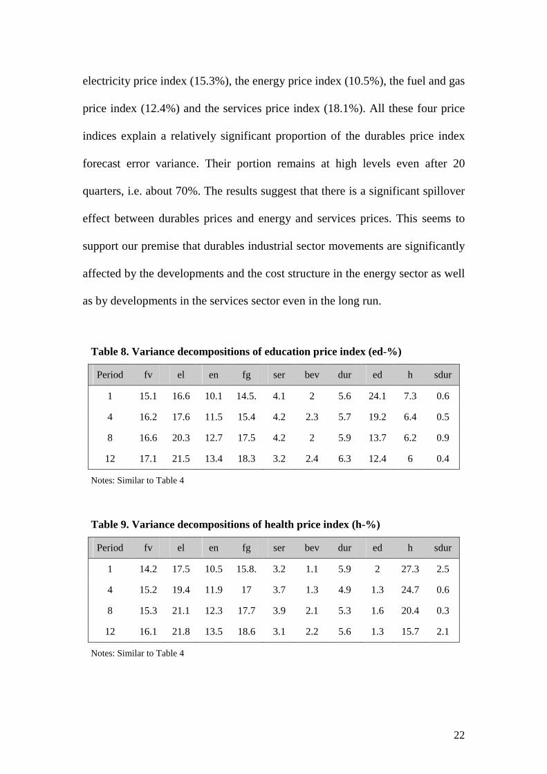
electricity price index (15.3%), the energy price index (10.5%), the fuel and gas

price index (12.4%) and the services price index (18.1%). All these four price

indices explain a relatively significant proportion of the durables price index

forecast error variance. Their portion remains at high levels even after 20

quarters, i.e. about 70%. The results suggest that there is a significant spillover

effect between durables prices and energy and services prices. This seems to

support our premise that durables industrial sector movements are significantly

affected by the developments and the cost structure in the energy sector as well

as by developments in the services sector even in the long run.

Table 8. Variance decompositions of education price index (ed-%)


1 15.1 16.6 10.1 14.5. 4.1 2 5.6 24.1 7.3 0.6

4 16.2 17.6 11.5 15.4 4.2 2.3 5.7 19.2 6.4 0.5

8 16.6 20.3 12.7 17.5 4.2 2 5.9 13.7 6.2 0.9

12 17.1 21.5 13.4 18.3 3.2 2.4 6.3 12.4 6 0.4


Table 9. Variance decompositions of health price index (h-%)


1 14.2 17.5 10.5 15.8. 3.2 1.1 5.9 2 27.3 2.5

4 15.2 19.4 11.9 17 3.7 1.3 4.9 1.3 24.7 0.6

8 15.3 21.1 12.3 17.7 3.9 2.1 5.3 1.6 20.4 0.3

12 16.1 21.8 13.5 18.6 3.1 2.2 5.6 1.3 15.7 2.1


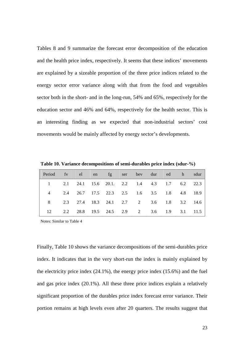
23

Tables 8 and 9 summarize the forecast error decomposition of the education

and the health price index, respectively. It seems that these indices’ movements

are explained by a sizeable proportion of the three price indices related to the

energy sector error variance along with that from the food and vegetables

sector both in the short- and in the long-run, 54% and 65%, respectively for the

education sector and 46% and 64%, respectively for the health sector. This is

an interesting finding as we expected that non-industrial sectors’ cost

movements would be mainly affected by energy sector’s developments.

Table 10. Variance decompositions of semi-durables price index (sdur-%)


1 2.1 24.1 15.6 20.1. 2.2 1.4 4.3 1.7 6.2 22.3

4 2.4 26.7 17.5 22.3 2.5 1.6 3.5 1.8 4.8 18.9

8 2.3 27.4 18.3 24.1 2.7 2 3.6 1.8 3.2 14.6

12 2.2 28.8 19.5 24.5 2.9 2 3.6 1.9 3.1 11.5


Finally, Table 10 shows the variance decompositions of the semi-durables price

index. It indicates that in the very short-run the index is mainly explained by

the electricity price index (24.1%), the energy price index (15.6%) and the fuel

and gas price index (20.1%). All these three price indices explain a relatively

significant proportion of the durables price index forecast error variance. Their

portion remains at high levels even after 20 quarters. The results suggest that

24

there is a significant spillover effect between semi-durables prices and energy

prices. This seems to support our premise that semi-durables industrial sector

movements are significantly affected by the developments and the cost

structure in the energy sector both in the short and in the long run.

4. Discussion of the Results

Our empirical analysis shows that the empirical findings have highlighted the

causality running from fuel prices towards the other CPI components. In other

words, any rises in fuel prices pass on to the remaining parts of the economy

and from the consumer standpoint (households and industry) the energy bill

grows, whereas from the production standpoint, firms have to content with a

rise in unit costs, and, therefore, in their charging prices. Thus, such rises in

fuel prices represent an inflationary shock that is accompanied by second-round

effects. More particularly, our results show that in Greece, any oil price

increases affect mainly the conditions of the supply side in the economy since

energy is the primary input of the production process (Greece is heavily

dependent on oil imports to satisfy their domestic needs for production and

consumption). As a result, the cost of production increases. Thus, our empirical

findings allow energy prices to affect the Phillips curve, which maps deviations

of actual inflation from targeted inflation (set by the European Central Bank) to

the current level of output gap, to capture inflationary effects in all sectors of

25

the economy, and, in turn, to change the trade-off between inflation and

unemployment in the Greek economy.

These empirical findings are also supported by the Real Business Cycle (RBC)

theory whereby energy price shocks are considered as supply or technological

regress. Moreover, following energy price rises, households may ask for

increasing wages to restore their purchasing power, leading to price-wage

loops. Next, turning to the firms, they can pass on such energy and wage rises

to selling prices, which generate upward revisions of higher price expectations,

which are diffused in all components of economic activity, especially in all

manufacturing and service sectors.

The above findings imply that Greek economic authorities could not afford

worrying only about growth and unemployment, but also about inflation,

though the participation in the Euroland was supposed to alleviate the most part

of this inflation burden. At the root of the inflation problem is the fact that

prices and, consequently, wages rise much faster than the country’s Eurozone

competitors. This loss of competitiveness can no longer be compensated for by

currency depreciation. Moreover, wage pressures and rigid labour laws

characterizing the Greek labour market do not help the competitiveness

problem either.

Over time, inflation must be kept at low levels; that means that the economy

will see its debt burden worsened by deflation. However, deflation is rather a

26

painful process, which invariably takes a toll on growth and employment, a fact

that is expected to aggravate the debt burden in the future along with all the

recent negative fiscal developments. The Greek inflation problem can been

handled either through the channel of tax policy or, primarily, through the

deregulation and the opening of certain sectors in the economy characterized by

monopolistic or oligopolistic conditions as well as through a stronger labour

market flexibility (the so called structural economic changes). In particular, the

lack of open markets impedes competition from driving down prices. Greece is

considered to be the least ‘trade open’ economy among the remaining European

Union members, with trade covering only 15% of GDP. This feature of the

economy makes the life of domestic monopolistic markets easier, as

competition from abroad is restricted, leading to prices acceleration. As an

alternative, the euro area members could adopt more expansionary economic

policies. However, this policy option is an anathema as the followers of

‘inflation scepticism’ will never adopt such an option.

5. Conclusions and Policy Implications

This empirical study examined the relationship among various CPI components

for the case of the Greek economy. The analysis covered the period 1981 to

2009 (on a quarterly basis) and considered the CPI components price indices.

Our results indicated the primary price movements are transmitted from the

27

energy price indices, i.e. the electricity price index, the energy price index and

the fuels and gas price index, while a secondary role also comes from the food

and vegetables price index along with the services price index.

In addition and in terms of causality, the evidence indicates that there is a

unidirectional transmission of energy prices disturbance to the remaining CPI

components, while innovations (shocks) to the remaining CPI components did

not have any significant effect on all indices. The implication is that certain

sectors are shielded from disturbances originating sectors excluding those

related to energy prices. These empirical results are crucial for policy makers as

well as for macroeconomists, since they support the pass-through effect of oil

prices into inflation and, therefore, the efficiency of policy makers to keep

inflation under control.

28

References

Apergis, N. (2010), The domestic Balassa-Samuelson effect of inflation, Working Paper, Hellenic Observatory, London School of Economics, London.

Barro, R.J. (1991), Economic growth in a cross-section of countries’, Quarterly Journal of Economics 106, pp. 407-443.

Barsky, R. and Kilian, L. (2004), Oil and the macroeconomy since the 1970s, NBER Working Paper, No. 10855.

Bayoumi, T. and Eichengreen, B. (1992), Shocking aspects of monetary unification’, NBER Working Paper No. 3949.

Blanchard, O. J. and Gali, J. (2007) ‘The macroeconomic effects of oil shocks: Why are the 2000s so different from the 1970s?’, NBER Working Paper No. 13368.

Blanchard, O. J. and Quah, D. (1989), The dynamic effects of aggregate demand and supply disturbances, American Economic Review, pp. 655-673.

Chen, S. S. (2009) ‘Oil price pass-through into inflation’, Energy Economics 31, pp.126-133.

Den Noord, P. J. and Andre, C. (2007) ‘Why has core inflation remained so muted in the face of the oil shock?’, SSRN=http://papers.ssrn.com/sol13/papers.cfm?text_id=1618189.

Dickey, D. A. and Fuller, W. A. (1981), Likelihood ratio statistics for autoregressive time series with unit root, Econometrica 49, pp. 1057-1072.

ECB (2005), Does product market competition reduce inflation? Evidence from EU countries and sectors, Working Paper No. 453.

Enders, W. (1995), Applied Econometric Time Series, New York: Wiley.

Ferderer, J. P. (1996), Oil price volatility and the macroeconomy, Journal of Macroeconomics 18, pp. 1-26.

Frankel, J.A. and Romer, D. (1999), Does trade cause growth?, American Economic Review 89, pp. 379-399.

Gregorio, J. D., Landerretche, O. and Nelson, C. (2007) ‘Another pass-through bites the dust? Oil prices and inflation’, Working Paper, Central Bank of Chile.

Grier, K. and Tullock, G. (1989), Empirical analysis of cross-national economic growth, 1951-1980, Journal of Monetary Economics 24, pp. 259-276.

29

Gulasekaran, R. (2004), Effects of temporal aggregation and systematic sampling on model dynamics and causal inference, Working Paper, National University of Singapore.

Gulasekaran, R. and T. Abeysinghe, (2002), The distortionary effects of temporal aggregation on Granger causality, Working Paper, National University of Singapore.

Hamilton, J. D. (1994), Time Series Analysis, Princeton University Press.

Hooker, M. A. (2002), Are oil shocks inflationary? asymmetric and nonlinear specifications versus changes in regime, Journal of Money, Credit and Banking 34, pp. 540-561.

King, R.G. and Levine, R. (1993), Finance and growth: Schumpeter might be right, Quarterly Journal of Economics 108, pp. 717-737.

LeBlanc, M. and Chinn, M. D. (2004), Do high oil prices presage inflation? The evidence from G5 countries, Business Economics 34, pp. 38-48.

Levine, R. and Zervos, S.J. (1993), What we have learned about policy and growth from cross-country regressions?, American Economic Review 83, pp. 426-430.

Levine, R. and Renelt, D (1992), A sensitivity analysis of cross-country growth regressions, American Economic Review 82, pp. 942-963.

Quah, D. and Vahey, S. P. (1995), Measuring core inflation, The Economic Journal 105, pp. 1130- 1144.

Sims, C. A. (1980), Macroeconomics and reality, Econometrica 48, pp. 1-48.

30

1

Other papers in this series 43 Apergis, Nicholas, Characteristics of inflation in Greece: mean spillover effects among

CPI components, January 2011

42 Kazamias, George, From Pragmatism to Idealism to Failure: Britain in the Cyprus crisis of 1974, December 2010

41 Dimas, Christos, Privatization in the name of ‘Europe’. Analyzing the telecoms privatization in Greece from a ‘discursive institutionalist’ perspective, November 2010

40 Katsikas, Elias and Panagiotidis, Theodore, Student Status and Academic Performance: an approach of the quality determinants of university studies in Greece, October 2010

39 Karagiannis, Stelios, Panagopoulos, Yannis, and Vlamis, Prodromos, Symmetric or Asymmetric Interest Rate Adjustments? Evidence from Greece, Bulgaria and Slovenia, September 2010

38 Pelagidis, Theodore, The Greek Paradox of Falling Competitiveness and Weak Institutions in a High GDP Growth Rate Context (1995-2008), August 2010

37 Vraniali, Efi, Rethinking Public Financial Management and Budgeting in Greece: time to reboot?, July 2010

36 Lyberaki, Antigone, The Record of Gender Policies in Greece 1980-2010: legal form and economic substance, June 2010

35 Markova, Eugenia, Effects of Migration on Sending Countries: lessons from Bulgaria, May 2010

34 Tinios, Platon, Vacillations around a Pension Reform Trajectory: time for a change?, April 2010

33 Bozhilova, Diana, When Foreign Direct Investment is Good for Development: Bulgaria’s accession, industrial restructuring and regional FDI, March 2010

32 Karamessini, Maria, Transition Strategies and Labour Market Integration of Greek University Graduates, February 2010

31 Matsaganis, Manos and Flevotomou, Maria, Distributional implications of tax evasion in Greece, January 2010

30 Hugh-Jones, David, Katsanidou, Alexia and Riener, Gerhard, Political Discrimination in the Aftermath of Violence: the case of the Greek riots, December 2009

29 Monastiriotis, Vassilis and Petrakos, George Local sustainable development and spatial cohesion in the post-transition Balkans: policy issues and some theory, November 2009

28 Monastiriotis, Vassilis and Antoniades, Andreas Reform That! Greece’s failing reform technology: beyond ‘vested interests’ and ‘political exchange’, October 2009

27 Chryssochoou, Dimitris, Making Citizenship Education Work: European and Greek perspectives, September 2009

26 Christopoulou, Rebekka and Kosma, Theodora, Skills and Wage Inequality in Greece:Evidence from Matched Employer-Employee Data, 1995-2002, May 2009

25 Papadimitriou, Dimitris and Gateva, Eli, Between Enlargement-led Europeanisation and Balkan Exceptionalism: an appraisal of Bulgaria’s and Romania’s entry into the European Union, April 2009

24 Bozhilova, Diana, EU Energy Policy and Regional Co-operation in South-East Europe: managing energy security through diversification of supply?, March 2009

23 Lazarou, Elena, Mass Media and the Europeanization of Greek-Turkish Relations: discourse transformation in the Greek press 1997-2003, February 2009

22 Christodoulakis, Nikos, Ten Years of EMU: convergence, divergence and new policy priorities, January 2009

2

21 Boussiakou, Iris Religious Freedom and Minority Rights in Greece: the case of the Muslim minority in western Thrace, December 2008

20 Lyberaki, Antigone “Deae ex Machina”: migrant women, care work and women’s employment in Greece, November 2008

19 Ker-Lindsay, James, The security dimensions of a Cyprus solution, October 2008

18 Economides, Spyros, The politics of differentiated integration: the case of the Balkans, September 2008

17 Fokas, Effie, A new role for the church? Reassessing the place of religion in the Greek public sphere, August 2008

16 Klapper, Leora and Tzioumis, Konstantinos, Taxation and Capital Structure: evidence from a transition economy, July 2008

15 Monastiriotis, Vassilis, The Emergence of Regional Policy in Bulgaria: regional problems, EU influences and domestic constraints, June 2008

14 Psycharis, Yannis, Public Spending Patterns:The Regional Allocation of Public Investment in Greece by Political Period, May 2008

13 Tsakalotos, Euclid, Modernization and Centre-Left Dilemmas in Greece: the Revenge of the Underdogs, April 2008

12 Blavoukos, Spyros and Pagoulatos, George, Fiscal Adjustment in Southern Europe: the Limits of EMU Conditionality, March 2008

11 Featherstone, Kevin, ‘Varieties of Capitalism’ and the Greek case: explaining the constraints on domestic reform?, February 2008

10 Monastiriotis, Vassilis, Quo Vadis Southeast Europe? EU Accession, Regional Cooperation and the need for a Balkan Development Strategy, January 2008

9 Paraskevopoulos, Christos, Social Capital and Public Policy in Greece, December 2007

8 Anastassopoulos George, Filippaios Fragkiskos and Phillips Paul, An ‘eclectic’ investigation of tourism multinationals’ activities: Evidence from the Hotels and Hospitality Sector in Greece, November 2007

7 Watson, Max, Growing Together? – Prospects for Economic Convergence and Reunification in Cyprus, October 2007

6 Stavridis, Stelios, Anti-Americanism in Greece: reactions to the 11-S, Afghanistan and Iraq, September 2007

5 Monastiriotis, Vassilis, Patterns of spatial association and their persistence across socio-economic indicators: the case of the Greek regions, August 2007

4 Papaspyrou, Theodoros, Economic Policy in EMU: Community Framework, National Strategies and Greece, July 2007

3 Zahariadis, Nikolaos, Subsidising Europe’s Industry: is Greece the exception?, June 2007

2 Dimitrakopoulos, Dionyssis, Institutions and the Implementation of EU Public Policy in Greece: the case of public procurement, May 2007

1 Monastiriotis, Vassilis and Tsamis, Achilleas, Greece’s new Balkan Economic Relations: policy shifts but no structural change, April 2007

Other papers from the Hellenic Observatory Papers from past series published by the Hellenic Observatory are available at http://www.lse.ac.uk/collections/hellenicObservatory/pubs/DP_oldseries.htm

Characteristics of inflation in Greece: Mean Spillover ...eprints.lse.ac.uk/32597/1/GreeSE_No43.pdf · Characteristics of inflation in Greece: ... the impact of oil price shocks on

Documents