University of Wollongong University of Wollongong Research Online Research Online University of Wollongong Thesis Collection 2017+ University of Wollongong Thesis Collections 2019 Characteristic Classes of Foliated Manifolds in Noncommutative Characteristic Classes of Foliated Manifolds in Noncommutative Geometry Geometry Lachlan E. MacDonald Follow this and additional works at: https://ro.uow.edu.au/theses1 University of Wollongong University of Wollongong Copyright Warning Copyright Warning You may print or download ONE copy of this document for the purpose of your own research or study. The University does not authorise you to copy, communicate or otherwise make available electronically to any other person any copyright material contained on this site. You are reminded of the following: This work is copyright. Apart from any use permitted under the Copyright Act 1968, no part of this work may be reproduced by any process, nor may any other exclusive right be exercised, without the permission of the author. Copyright owners are entitled to take legal action against persons who infringe their copyright. A reproduction of material that is protected by copyright may be a copyright infringement. A court may impose penalties and award damages in relation to offences and infringements relating to copyright material. Higher penalties may apply, and higher damages may be awarded, for offences and infringements involving the conversion of material into digital or electronic form. Unless otherwise indicated, the views expressed in this thesis are those of the author and do not necessarily Unless otherwise indicated, the views expressed in this thesis are those of the author and do not necessarily represent the views of the University of Wollongong. represent the views of the University of Wollongong. Research Online is the open access institutional repository for the University of Wollongong. For further information contact the UOW Library: [email protected] brought to you by CORE View metadata, citation and similar papers at core.ac.uk provided by Research Online

Welcome message from author
This document is posted to help you gain knowledge. Please leave a comment to let me know what you think about it! Share it to your friends and learn new things together.
Transcript

University of Wollongong University of Wollongong
Research Online Research Online
University of Wollongong Thesis Collection 2017+ University of Wollongong Thesis Collections
2019
Characteristic Classes of Foliated Manifolds in Noncommutative Characteristic Classes of Foliated Manifolds in Noncommutative
Geometry Geometry
Lachlan E. MacDonald
Follow this and additional works at: https://ro.uow.edu.au/theses1
University of Wollongong University of Wollongong
Copyright Warning Copyright Warning
You may print or download ONE copy of this document for the purpose of your own research or study. The University
does not authorise you to copy, communicate or otherwise make available electronically to any other person any
copyright material contained on this site.
You are reminded of the following: This work is copyright. Apart from any use permitted under the Copyright Act
1968, no part of this work may be reproduced by any process, nor may any other exclusive right be exercised,
without the permission of the author. Copyright owners are entitled to take legal action against persons who infringe
their copyright. A reproduction of material that is protected by copyright may be a copyright infringement. A court
may impose penalties and award damages in relation to offences and infringements relating to copyright material.
Higher penalties may apply, and higher damages may be awarded, for offences and infringements involving the
conversion of material into digital or electronic form.
Unless otherwise indicated, the views expressed in this thesis are those of the author and do not necessarily Unless otherwise indicated, the views expressed in this thesis are those of the author and do not necessarily
represent the views of the University of Wollongong. represent the views of the University of Wollongong.
Research Online is the open access institutional repository for the University of Wollongong. For further information contact the UOW Library: [email protected]
brought to you by COREView metadata, citation and similar papers at core.ac.uk
provided by Research Online
Characteristic Classes of Foliated Manifolds inNoncommutative Geometry
Lachlan E. MacDonald
Supervisor:Associate Professor A. Rennie
Co-supervisor:Dr. G. Wheeler
This thesis is presented as part of the requirements for the conferral of the degree:
Doctor of Philosophy (Mathematics)
The University of WollongongSchool of School of Mathematics and Applied Statistics
August 2019

Declaration
I, Lachlan E. MacDonald, declare that this thesis submitted in partial fulfilment of the
requirements for the conferral of the degree Doctor of Philosophy (Mathematics), from the
University of Wollongong, is wholly my own work unless otherwise referenced or acknowl-
edged. This document has not been submitted for qualifications at any other academic
institution.
Lachlan E. MacDonald
November 7, 2019


Abstract
We present a detailed account of the well-known theory of foliated manifolds, their holon-
omy groupoids and their characteristic classes using Chern-Weil theory. We give, for the
first time, a characteristic map from the cohomology of the Weil algebra of the general
linear group into the cohomology of the full holonomy groupoid of the transverse frame
bundle of a transversely orientable foliated manifold. From our characteristic map, we
derive a codimension 1 Godbillon-Vey cyclic cocycle for the smooth algebra of the trans-
verse frame holonomy groupoid that is the non-etale analogue of the formula given by
Connes and Moscovici [58]. Following this, for transversely orientable foliations of arbi-
trary codimension, we construct unbounded Kasparov modules that are equivariant for
actions of the full holonomy groupoid. Finally we show that in codimension 1, one of these
Kasparov modules can be used to construct a semifinite spectral triple for the C∗-algebra
of the transverse frame holonomy groupoid. We prove an index theorem identifying this
semifinite spectral triple with our Godbillon-Vey cyclic cocycle, and relate our results
to earlier work by Connes. We give in the appendix the required details for equivariant
KK-theory for non-Hausdorff groupoids, which do not currently exist in the literature.
v

vi
Acknowledgments
This research was funded by an Australian Postgraduate Award (now a Research Train-
ing Program scholarship). I thank the Australian Department of Education and the
University of Wollongong for their support. I also thank the University of Wollongong
for financial support for conference travel.
My deepest thanks go to Adam Rennie, my primary supervisor for this thesis, without
whose expertise, patience, and relentless optimism my research would not have been
possible. I wish to thank him especially for the vast amount of time he has spent reading
and editing my work. My thesis has been further improved as a consequence of a thorough
reading by the examiners, Moulay Benameur and Alexander Gorokhovsky, whom I thank
for their thoughtful comments and corrections. I would also like to thank my cosupervisor
Glen Wheeler for insight into the geometric aspects of foliations. Those parts of my
research conducted in Australia have additionally benefited from discussions with Alan
Carey, Mathai Varghese, Ryszard Nest, and Bram Mesland.
I have been privileged to attend a number of conferences during my candidature. I
am grateful to the Australian Mathematical Sciences Institute for funding travel and
accommodation for both the MATRIX conference “Refining C∗-algebraic invariants for
dynamics using KK-theory” in Creswick in 2016, and for the “Australia-China conference
in Noncommutative Geometry and related areas” at the University of Adelaide in 2017. I
would also like to thank the Institute for Geometry and its Applications at the University
of Adelaide for funding travel and accommodation for the second of these conferences.
During the last few months of 2018, I enjoyed the great privilege of travelling to France
to visit Moulay Benameur at the Universite de Montpellier. I am immensely grateful
to Moulay for his hospitality, offers of financial support, and many enormously helpful
discussions. I am grateful also to Paulo Carillo Rouse for the invitation to talk at the
ANR SINGSTAR conference “Index Theory: Interactions and Applications”, and for the
accommodation and lunches at the conference. I would also like to express sincere thanks
to Michel Hilsum and Robert Yuncken for invitations to speak at the Seminaire d’Algebres
d’Operateurs at the Universite Paris Diderot, and at the Seminaire et Groupe de travail
GAAO at the Universite Clermont Auvergne respectively, and for providing support for
travel and accommodation. My research while in France has benefited from discussions
with Moulay, Michel and Robert, as well as Iakovos Androulidakis and Georges Skandalis.
vii
viii
While in Europe, I also had the wonderful opportunity to attend the “Bivariant K-
theory in geometry and physics” conference held at the Erwin Schrodinger Institute at
the Universitat Wien. I thank Adam Rennie and Alan Carey for travel funding, and I
thank the Erwin Schrodinger Institute for financial support. I must also thank Magnus
Goeffeng for inviting me to Chalmers University of Technology, for organising travel and
accommodation, and for a week’s worth of his sharing of mathematical insight.
My close friends and loved ones deserve deep thanks. My family, for their unceasing
and selfless love and support, without which my life would be infinitely poorer. My
good friend and fellow doctoral candidate Alex Mundey, for being an endless source
of stimulating discussion both mathematical and otherwise. My housemates (old and
current) Jason, Chris, and Dave for being the brothers I never had. My oldest friend
Geoffrey for his consistent friendship and intellectual discussions. And my wonderful
girlfriend Nina for her warmth, patience and love, and for always challenging me.
Finally I would like to acknowledge the great privilege with which I was brought into
the world - at a beautiful time (referred to by Adam Rennie as “after the fall of the wall
and before the fall of the towers”), in a beautiful place (the southeast coast of Australia)
and to beautiful people (my loving family). I am deeply and humbly grateful for the
opportunities afforded to me by these favourable circumstances, without which I would
not be where I am today.
Contents
Abstract v
1 Introduction 1
1.1 The story so far . . . . . . . . . . . . . . . . . . . . . . . . . . . . . . . . 1
1.1.1 Foliations and their characteristic classes . . . . . . . . . . . . . . 1
1.1.2 Models for the leaf space and dynamics . . . . . . . . . . . . . . . 4
1.1.3 Foliations as noncommutative geometries . . . . . . . . . . . . . . 6
1.2 The present thesis . . . . . . . . . . . . . . . . . . . . . . . . . . . . . . . 10
2 Foliated manifolds and characteristic classes 13
2.1 First definitions and examples . . . . . . . . . . . . . . . . . . . . . . . . 13
2.2 The local structure of a foliated manifold . . . . . . . . . . . . . . . . . . 18
2.3 The classical Godbillon-Vey invariant . . . . . . . . . . . . . . . . . . . . 24
2.4 Chern-Weil theory and secondary characteristic classes . . . . . . . . . . 29
2.4.1 Chern-Weil theory for vector bundles . . . . . . . . . . . . . . . . 29
2.4.2 Chern-Weil theory for foliations . . . . . . . . . . . . . . . . . . . 35
2.5 The Godbillon-Vey invariant using Chern-Weil theory . . . . . . . . . . . 39
3 Holonomy and related constructions 43
3.1 Holonomy . . . . . . . . . . . . . . . . . . . . . . . . . . . . . . . . . . . 43
3.1.1 Holonomy diffeomorphisms and their germs . . . . . . . . . . . . 44
3.1.2 Differential topology of the holonomy groupoid . . . . . . . . . . 50
3.2 Equivariant bundles . . . . . . . . . . . . . . . . . . . . . . . . . . . . . . 55
3.2.1 The frame bundle . . . . . . . . . . . . . . . . . . . . . . . . . . . 59
3.2.2 Jets and jet groups . . . . . . . . . . . . . . . . . . . . . . . . . . 65
3.2.3 Jet bundles . . . . . . . . . . . . . . . . . . . . . . . . . . . . . . 67
3.3 Algebras associated to the holonomy groupoid . . . . . . . . . . . . . . . 81
3.3.1 The smooth convolution algebra . . . . . . . . . . . . . . . . . . . 82
3.3.2 The C∗-algebra . . . . . . . . . . . . . . . . . . . . . . . . . . . . 85
ix

x CONTENTS
4 Characteristic classes on the holonomy groupoid 89
4.1 Chern-Weil homomorphism for Lie groupoids . . . . . . . . . . . . . . . . 90
4.2 Characteristic map for foliated manifolds . . . . . . . . . . . . . . . . . . 99
4.3 The codimension 1 Godbillon-Vey cyclic cocycle . . . . . . . . . . . . . . 103
5 Index theorem 113
5.1 The Connes Kasparov module . . . . . . . . . . . . . . . . . . . . . . . . 113
5.2 The Vey Kasparov module . . . . . . . . . . . . . . . . . . . . . . . . . . 120
5.3 An index theorem for the Godbillon-Vey cyclic cocycle . . . . . . . . . . 126
5.3.1 The spectral triple . . . . . . . . . . . . . . . . . . . . . . . . . . 126
5.3.2 The index theorem . . . . . . . . . . . . . . . . . . . . . . . . . . 129
A Noncommutative index theory 137
A.1 Index pairings and KK-theory . . . . . . . . . . . . . . . . . . . . . . . . 137
A.1.1 Gradings, Hilbert modules and operators thereon . . . . . . . . . 137
A.1.2 K∗, K∗ and the index pairing . . . . . . . . . . . . . . . . . . . . 142
A.1.3 KK-theory: the bounded picture . . . . . . . . . . . . . . . . . . 146
A.1.4 KK-theory: the unbounded picture and spectral triples . . . . . . 147
A.2 Cyclic cohomology and index formulae . . . . . . . . . . . . . . . . . . . 151
A.2.1 Cyclic cohomology . . . . . . . . . . . . . . . . . . . . . . . . . . 152
A.2.2 The local index formula . . . . . . . . . . . . . . . . . . . . . . . 153
B Groupoids and equivariant KK-theory 159
B.1 Groupoids . . . . . . . . . . . . . . . . . . . . . . . . . . . . . . . . . . . 160
B.2 Upper-semicontinuous bundles . . . . . . . . . . . . . . . . . . . . . . . . 161
B.3 Groupoid actions on algebras and modules . . . . . . . . . . . . . . . . . 168
B.4 KKG-theory . . . . . . . . . . . . . . . . . . . . . . . . . . . . . . . . . . 171
B.5 The Kasparov product . . . . . . . . . . . . . . . . . . . . . . . . . . . . 174
B.6 Crossed products . . . . . . . . . . . . . . . . . . . . . . . . . . . . . . . 178
B.7 The descent map . . . . . . . . . . . . . . . . . . . . . . . . . . . . . . . 182
C Connections, curvature and holonomy 189
D Differential graded algebras 193
D.1 Differential graded algebras and their cohomology . . . . . . . . . . . . . 193
D.2 G-differential graded algebras . . . . . . . . . . . . . . . . . . . . . . . . 195
D.3 The Weil algebra of the general linear lie algebra . . . . . . . . . . . . . . 201

Chapter 1
Introduction
1.1 The story so far
1.1.1 Foliations and their characteristic classes
Geometrically speaking, a (regular) foliation F of a smooth n-dimensional manifold M
is a realisation of M as a “layered space”. One requires the layers of this foliation (called
leaves) to be immersed, connected submanifolds of M of the same dimension (say p ≤ n),
which fit together without intersection. More specifically, one requires M to look locally
like the product Rn = Rp×Rn−p, where the submanifolds Rp×z correspond to the
leaves of F - such local charts are called foliated charts. The pair (M,F) is referred to
as a foliated manifold. The dimension p of the leaves of (M,F) is referred to as the leaf
dimension, while the dimension q := n − p of the transverse space that is “left over” is
referred to as the codimension. Associated canonically to any foliated manifold (M,F)
is the leafwise tangent bundle T F ⊂ TM consisting of vectors tangent to leaves, and
the normal bundle N := TM/T F , which may be thought of as the “tangents to the
transverse directions”.
Examples of foliated manifolds can be found in many parts of mathematics and its
applications. In physics, for instance, the structure of a local region of spacetime is
modelled by a codimension 1 foliation of a 4-dimensional manifold. The leaves in this
case are the snapshots of some local region of space at particular instants in time, and
the way the leaves fit into the ambient manifold describes the evolution of space through
time. Frequently in cosmological models the hypothesis of global hyperbolicity is invoked,
which allows one to describe the global structure of spacetime in this manner as well.
Foliated manifolds also appear in the study of differential equations. An integrable,
first order, linear, ordinary differential equation (ODE), for instance, is associated with a
foliation of R2 by the integral curves of that ODE. More generally, and in more modern
language, a nonsingular system of first order linear partial differential equations (PDE)
on a manifold M is associated to a smooth subbundle E of TM . The famous Frobenius
1
2 CHAPTER 1. INTRODUCTION
theorem [34, Section 1.3] states that such a system is integrable, and produces therefore
a foliation of M by integral submanifolds, if and only if the smooth sections of E are
closed under Lie brackets. That the Frobenius theorem is an equivalence in fact allows us
to realise any foliation of a manifold M as the solution set of some system of sufficiently
nice PDE defined on M . Thus to study foliations of manifolds is to study the global
behaviour of solutions to systems of PDE on manifolds.
Despite their apparent ubiquity, the study of foliated manifolds in their own right
wasn’t initiated until the work of C. Ehresmann and G. Reeb in the mid twentieth century
[71]. Since then, research into the structure of foliated manifolds and their implications
for dynamics and topology has been intense and extensive. Of particular interest for
this thesis is the discovery due to C. Godbillon and J. Vey [81] of the Godbillon-Vey
invariant of any codimension 1 foliated manifold (M,F) whose normal bundle N is
orientable (foliations with orientable normal bundle are called transversely orientable).
Their construction is quite simple so we give it here.
One starts with a differential 1-form ω ∈ Ω1(M) which defines the foliation F in the
sense that it is nowhere vanishing, but is identically zero when evaluated on vectors in
T F . That such a form exists is guaranteed by the orientability of the normal bundle N .
A version of the Frobenius theorem then says that there exists a form η ∈ Ω1(M) such
that dω = η ∧ ω. Consequently
0 = d2ω = d(η ∧ ω) = dη ∧ ω − η ∧ η ∧ ω = dη ∧ ω.
Now the fact that ω is nowhere vanishing implies that dη = ω ∧ γ for some γ ∈ Ω1(M).
Therefore
d(η ∧ dη) = dη ∧ dη = ω ∧ γ ∧ ω ∧ γ = 0
so that η∧dη defines a class in the de Rham cohomology H3dR(M) of M , which Godbillon
and Vey show is independent of the choices of η and ω. The class
gv(M,F) := [η ∧ dη] ∈ H3dR(M) (1.1)
so obtained is known as the Godbillon-Vey invariant of (M,F).
In the decades that followed, the Godbillon-Vey invariant was the subject of intense
research. One of the directions this research took was in systematising the construction
of the Godbillon-Vey invariant so as to generalise it to foliations of higher codimension,
and to discover related invariants. Since the nineteen-seventies, two distinct but closely
related “roads” in this direction have been discovered: the “high road” of Gelfand-Fuks
cohomology, and the “low road” of Chern-Weil theory (the terminology in quotation
marks here is due to R. Bott, [26, p. 211]).
The Gelfand-Fuks approach has at its core the cohomology of Lie algebras of formal

1.1. THE STORY SO FAR 3
vector fields on Euclidean space, whose study was initiated by I. Gelfand and D. Fuks in
[77]. The Gelfand-Fuks approach is in a certain sense the deeper and more fundamental
of the two approaches (hence Bott’s terminology). On the other hand, in computing
representatives for the classes obtained using Gelfand-Fuks cohomology, one usually ends
up using the connection and curvature forms that are at the heart of Chern-Weil theory
anyway. Consequently in this thesis we will focus primarily on the “low road” of Chern-
Weil theory. The relevant Chern-Weil material is covered in detail in Chapter 2, but for
the sake of exposition we outline it below.
Let (M,F) be a foliated manifold of codimension q, and let I∗q (R) = R[c1, . . . , cq]
denote the ring generated by the invariant polynomials ck(A) := Tr(Ak) defined for A in
the general linear Lie algebra gl(q,R). Then given a connection ∇ on the normal bundle
N , with curvature R, one has the Chern-Weil homomorphism φ∇ : I∗q (R) → Ω∗(M)
defined by
I∗q (R) 3 ck 7→ ck(R) := Tr(Rk) ∈ Ω2k(M).
Every element in the image of φ∇ is closed under the exterior derivative d, so that φ∇
descends to a map I∗q (R) → H∗dR(M), and this map does not depend on the connection
chosen. The image of any such φ∇ in H∗dR(M) is called the Pontryagin ring associated to
N , and its elements referred to as the Pontryagin classes of N , with the image of each ck in
particular referred to as the kth Pontryagin class of N . The local structure of the foliation
then guarantees that we can choose a Bott connection ∇ = ∇[, characterised amongst all
connections on N by its coincidence with the trivial connection along sufficiently small
charts in leaves. By representing the Pontryagin classes of N using the curvature of a
Bott connection, Bott proved the following theorem.
Theorem 1.1.1 (Bott). Let (M,F) be a foliated manifold of codimension q. Then the
Pontryagin classes of the normal bundle N vanish in degree greater than 2q.
Theorem 1.1.1 is now known as Bott’s vanishing theorem. As has been known since
the work of S. S. Chern and J. Simons, [50], such vanishing phenomena imply the ex-
istence of new de Rham classes arising from certain transgressions of other cochains.
In the case of foliations specifically, the data pertaining to the Pontryagin classes and
their transgressions are encoded in a differential graded algebra WOq together with a
characteristic map
φ∇],∇[ : WOq → Ω∗(M) (1.2)
constructed from any Bott connection ∇[ and metric-compatible connection ∇] on N
(see Theorem 2.4.21). The induced map H∗(WOq) → H∗dR(M) does not depend on the
Bott connection or metric-compatible connection chosen. For codimension 1 transversely
orientable foliations, a clever choice of∇] and∇[ allows one to see the representative η∧dηof Equation (1.1) as the only non-Pontryagin cochain appearing in the image of φ∇],∇[ in

4 CHAPTER 1. INTRODUCTION
Ω∗(M). For a general foliation, those classes obtained from φ∇],∇[ that are not contained
in the Pontryagin ring of the normal bundle are called the secondary characteristic classes
associated to the foliation.
1.1.2 Models for the leaf space and dynamics
Since the secondary characteristic classes of a foliated manifold (M,F) arise from its nor-
mal bundle, one might expect them to have an interpretation as characteristic classes for
the “space of leaves” or “transverse space” M/F of the foliation. However the naıve def-
inition of M/F , as the quotient of M by the equivalence relation that identifies points in
the same leaf, produces a topologically pathological space that is not in general amenable
to any of the usual tools of algebraic topology, let alone those of differential geometry. The
notion of equivalence relation does, however, admit a more useful generalisation, namely
that of a groupoid. In short, a groupoid is a small category for which every morphism
has an inverse, and is fundamentally a dynamical object. The objects of a groupoid are
called its units, while the maps which assign to any morphism its domain and codomain
are called the source and range maps respectively. That foliations of manifolds ought to
be modelled using such objects was realised early on by A. Haefliger [89], whose insights
we now outline.
If Uα and Uβ are two sufficiently nice foliated charts in a codimension q foliated
manifold (M,F), with Uα ∩ Uβ 6= ∅, then from the transverse change of coordinates one
obtains a local diffeomorphism cαβ of Rq. Taking a sufficiently nice covering U := Uαα∈Aby such charts, one obtains a collection cαβα,β∈A of local diffeomorphisms of Rq such
that whenever Uα ∩ Uβ ∩ Uδ 6= ∅ one has
cαβ cβδ = cαδ. (1.3)
The local diffeomorphisms cαβ essentially describe the maps on transversals obtained by
following paths in leaves - that is, they describe the holonomy of the foliation. The
collection cαβα,β∈A is called the holonomy cocycle associated to the cover U .
Associated to the cover U is its Cech groupoid C U , whose units are the Uα and whose
morphisms are the nonempty intersections Uα ∩ Uβ. Taking the germs of all the local
diffeomorphisms cαβ associated to U gives, by Equation (1.3), a homomorphism of C Uinto the groupoid Γq of all germs of local diffeomorphisms of Rq. This homomorphism
is called a Haefliger cocycle for the manifold M , and its image in Γq will be denoted by
(M/F)U . In capturing all the transverse change of coordinate information in (M,F),
the groupoid (M/F)U is suitable for use as a model for the leaf space M/F .
In fact Γq is an etale groupoid, in the sense that it carries a natural topology for which
its range and source maps are local homeomorphisms. Haefliger constructs from Γq the
classifying space BΓq for codimension q foliations, with the property that if (M,F) is

1.1. THE STORY SO FAR 5
any codimension q foliation then there exists a map φF : M → BΓq that classifies the
foliation F up to (integrable) homotopy. One therefore obtains a map
φ∗F : H∗(BΓq)→ H∗(M)
that depends only on the (integrable) homotopy class of F , and, by naturality [23, p.
70], a map φ : H∗(WOq)→ H∗(BΓq) such that the diagram
H∗(WOq) H∗(M)
H∗(BΓq)
φ∇],∇[
φφ∗F
(1.4)
commutes.
Now the characteristic map φ : H∗(WOq) → H∗(BΓq) is, due to its generality, nec-
essarily rather abstract. Given a particular codimension q foliation (M,F) therefore,
with a sufficiently nice covering U by foliated charts, one may be interested in computing
explicit representatives of cohomology classes for the groupoid (M/F)U in terms of geo-
metric data on M . A reasonable approximation to this groupoid is simply the groupoid
obtained from an action of a discrete group Γ on a q-dimensional manifold V by diffeomor-
phisms. Conceptually, one is to regard V as the disjoint union of transversals obtained
from any sufficiently nice covering of M , while Γ is used to approximate the pseudogroup
of local diffeomorphisms obtained thereon by the transverse coordinate changes.
Bott [26, 27] and Thurston [149] both worked in this setting in the nineteen-seventies.
Of special interest to us is Bott’s production of explicit formulae for group cocycles
obtained by tracking the displacement of a volume form θ and an affine connection ∇ on
V under the action of Γ. In particular, if one takes V to be a 1-dimensional Riemannian
manifold with Riemannian volume form θ and Levi-Civita connection ∇, for f ∈ Γ one
defines µ(f) := (f ∗θ)/θ and has f ∗∇−∇ = d log µ(f). In this setting Bott obtains the
famous Bott-Thurston cocycle
ω(f1, f2) :=
∫V
(log µ(f1) d log µ(f2)− log µ(f2) d log µ(f1)
). (1.5)
Bott shows that all cocycles showing up in this manner can be obtained from the algebra
WOq using the methods of simplicial de Rham theory devised by J. Dupont [70], and
that the Bott-Thurston cocycle in particular corresponds to the Godbillon-Vey invariant
for a codimension 1 foliation. More recently, M. Crainic and I. Moerdijk [64] have used
similar methods to derive analogous formulae for the etale groupoid (M/F)U associated
to any foliated manifold (M,F) with sufficiently nice covering U .
6 CHAPTER 1. INTRODUCTION
While the etale groupoids that have been traditionally used to study foliations have
proved powerful in studying the transverse structure of foliations, they are geometrically
suboptimal because they are blind to leafwise geometry. In the early nineteen-eighties,
H. E. Winkelnkemper gave a construction of the full holonomy groupoid G of any foliated
manifold (M,F) [153]. Winkelnkemper presents the full holonomy groupoid G as the
space of all paths in leaves of F , modulo the equivalence relation that identifies two paths
if and only if they induce the same holonomy maps on local transversals. While no longer
an etale groupoid, nor even necessarily Hausdorff, the full holonomy groupoid is Morita
equivalent to the etale groupoid (M/F)U obtained from a sufficiently nice covering U [63],
and is therefore cohomologically the same. Despite its advantages in being a completely
global object that captures both leafwise geometry and foliation dynamics simultaneously,
the full holonomy groupoid has seen almost no use in the study of the characteristic
classes of foliations. As will be shown in this thesis, translating the existing theory of
characteristic classes of foliations into the language of the full holonomy groupoid gives
rise to surprising new geometric interpretations of old formulae.
1.1.3 Foliations as noncommutative geometries
The study of foliated manifolds as noncommutative geometries starts with A. Connes’ in-
dex theorem for measured foliations [51], namely those foliations that admit a holonomy-
invariant transverse measure. Let us recall Connes’ result. As elucidated by the work of
D. Ruelle and D. Sullivan [143], a holonomy-invariant transverse measure ν for a com-
pact foliated manifold (M,F) is associated to a closed de Rham current, defining a class
Cν ∈ HdRdim(F)(M) in de Rham homology. If D is a leafwise-elliptic operator on (M,F),
then associated to D is an elliptic operator DL on each leaf L of F and one can make
sense of the quantity
dimν(ker(D)) =
∫dim(ker(DL)) dν(L).
Consequently one can form the ν-analytic index
indexν(D) := dimν(ker(D))− dimν(ker(D∗)).
Letting ch(D) and Td(M) denote the Chern class of D and the Todd class of M respec-
tively, Connes shows that the ν-analytic index of D can be computed by the topological
formula
indexν(D) = 〈ch(D) Td(M), Cν〉.
Note that the proof of Connes’ index theorem for measured foliations, since it concerns
leafwise differential operators, relies fundamentally on Winkelnkemper’s full holonomy

1.1. THE STORY SO FAR 7
groupoid.
To extend Connes’ remarkable result for measured foliations to foliations that are not
necessarily endowed with an invariant transverse measure, one requires noncommutative-
geometric tools. The first required tool is the reduced C∗-algebra C∗r (G) of the (generally
non-Hausdorff) full holonomy groupoid, defined by Connes [53] in a manner that closely
resembles the famous construction of J. Renault [141] for Hausdorff groupoids. The
algebra C∗r (G) is a noncommutative geometry that models the leaf space of the foliation.
The second is the powerful bivariant K-theory defined by Kasparov [105]. Using these
tools, Connes and G. Skandalis proved the longitudinal index theorem for foliations in
their groundbreaking paper [61]. Their theorem is one of the first applications of truly
noncommutative tools to solve a geometric problem.
Theorem 1.1.2 (Connes-Skandalis). Let (M,F) be a compact, foliated manifold, and
let D be a longitudinal elliptic pseudodifferential operator, with symbol class [σD] ∈K0(T ∗F). Then
indexa(D) = indext([σD]) (1.6)
as elements of K0(C∗r (G)).
In Theorem 1.1.2, the analytic index indexa(D) can be thought of as the pairing of
the class in K0(C(M)) defined by the trivial complex line bundle with the class in the
Kasparov group KK0(C(M), C∗r (G)) defined by D. The topological index indext on the
other hand is a map from K0(T ∗F) to K0(C∗r (G)) defined via an embedding of M into
Euclidean space in a manner reminiscient of the topological index of Atiyah and Singer
[11]. If (M,F) admits an invariant transverse measure ν, one obtains a trace τν on C∗r (G)
and hence a map (τν)∗ on K0(C∗r (G)). Applying (τν)∗ to both sides of Equation (1.6) one
recovers Connes’ index theorem for measured foliations. The longitudinal index theorem
has inspired a great deal of mathematical research in the decades since its publication
[33, 92, 17, 84, 18, 20, 46, 16].
Connes and Skandalis also show that the assembly map for the holonomy groupoid of
a foliation can be realised as a longitudinal index map. More specifically, associated to the
holonomy groupoid G of any foliated manifold (M,F) one has the Z2-graded geometric
groups K∗,τ (B G), whose basic cycles are triples (X,E, f), where X is a smooth, compact
manifold, E is a complex vector bundle on X, and f is a smooth, K-oriented map from
X to the space of leaves M/F (see [53] for more detail). Given any such triple we see
that E defines a class [E] ∈ K0(X), while in [61] it is shown that the K-oriented map
f is associated to a class f ! ∈ KK(C(X), C∗r (G)). One then obtains the assembly map
µ : K∗,τ (B G)→ K∗(C∗r (G)) using the Kasparov product
µ([(X,E, f)]) := [E]⊗C(X) f ! ∈ K∗(C∗r (G)).

8 CHAPTER 1. INTRODUCTION
The assembly map µ provides a recipe for constructing classes in the analytic groups
K∗(C∗r (G)) from geometric data.
Of course the longitudinal theory is only one “half” of the theory of foliated manifolds.
In his paper [55], Connes shows how to realise transverse geometric phenomena, for
instance the transverse fundamental class and the secondary characteristic classes, in the
noncommutative setting of cyclic cohomology. To emphasise the transverse nature of
his constructions (and also perhaps due to constraints on the mathematical technology
available at the time), Connes models the holonomy groupoid G by a discrete group Γ
acting by diffeomorphisms on a q-dimensional manifold V in a similar manner to Bott
and Thurston. One of the major technical feats of this paper is Connes’ solution to
the problem of having no metric structure on V that is preserved by the action of Γ.
Connes’ approach is to consider a particular fibre bundle W over V - the “bundle of
metrics”, which carries a natural action of Γ as well as a tautological “almost-invariant”
Riemannian structure. Using Γ-equivariant KK-theory, Connes lifts K-theoretic data
for the algebra C0(V ) o Γ to the algebra C0(W ) o Γ where the problem can be solved.
To date, Connes’ “bundle of metrics” remains the best solution to doing index theory in
the presence of a non-isometric action.
Another of the landmark achievements of [55] is the realisation of secondary charac-
teristic classes as functionals on K-theory. This requires some setup. Let π : EΓ → BΓ
denote the universal principal Γ-bundle over the classifying space BΓ of Γ, and let
VΓ := V ×ΓEΓ be the homotopy quotient (which is the classifying space for the groupoid
V o Γ). The Γ-equivariant vector bundle T ∗V over V induces a vector bundle τ on VΓ,
and we let K∗,τ (VΓ) denote the K-homology of the space VΓ twisted by the bundle τ .
By the results of [14] we have an assembly map µ : K∗,τ (VΓ) → K∗(C0(V ) o Γ), and
we let Φ ch : K∗,τ (VΓ) → H∗(VΓ) denote the Chern character (the Φ here is a Thom
isomorphism to “untwist” by τ , see [55, Section 6]). Finally let Bπ : VΓ → BΓq denote
the classifying map corresponding to the inclusion V oΓ→ Γq into the groupoid of germs
of all local diffeomorphisms of Rq. We then have the following.
Theorem 1.1.3. [55] Regard H∗(WOq) as a subring of H∗(BΓq) as in the diagram (1.4).
Then for any ω ∈ H∗(WOq) there exists a linear map ϕω : K∗(C0(V )oΓ)→ C such that
ϕω(µ(x)) = 〈Φ ch(x), (Bπ)∗ω〉
for all x ∈ K∗,τ (VΓ).
Actually Theorem 1.1.3 given above is, for the sake of simplicity, slightly different to
Connes’ [55, Theorem 7.15], however by [14, Lemma 1], Theorem 1.1.3 and [55, Theorem
7.15] coincide when Γ is torsion-free. Connes’ proof is rather nonconstructive: it uses
Γ-equivariant KK-classes for higher order jet bundles, whose existence is a consequence
1.1. THE STORY SO FAR 9
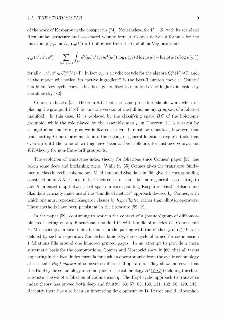
of the work of Kasparov in the conspectus [74]. Nonetheless, for V = S1 with its standard
Riemannian structure and associated volume form µ, Connes derives a formula for the
linear map ϕgv on K0(C0(V ) o Γ) obtained from the Godbillon-Vey invariant:
ϕgv(a0, a1, a2) =∑
g0g1g2=1
∫S1
a0(g0)a1(g1)a2(g2)(
log µ(g1) d log µ(g2)− log µ(g2) d log µ(g1))
for all a0, a1, a2 ∈ C∞c (V )oΓ. In fact ϕgv is a cyclic cocycle for the algebra C∞c (V )oΓ, and,
as the reader will notice, its “active ingredient” is the Bott-Thurston cocycle. Connes’
Godbillon-Vey cyclic cocycle has been generalised to manifolds V of higher dimension by
Gorokhovsky [82].
Connes indicates [55, Theorem 8.1] that the same procedure should work when re-
placing the groupoid V oΓ by an etale version of the full holonomy groupoid of a foliated
manifold. In this case, VΓ is replaced by the classifying space B G of the holonomy
groupoid, while the role played by the assembly map µ in Theorem 1.1.3 is taken by
a longitudinal index map as we indicated earlier. It must be remarked, however, that
transporting Connes’ arguments into the setting of general foliations requires tools that
even up until the time of writing have been at best folklore, for instance equivariant
KK-theory for non-Hausdorff groupoids.
The evolution of transverse index theory for foliations since Connes’ paper [55] has
taken some deep and intriguing turns. While in [55] Connes gives the transverse funda-
mental class in cyclic cohomology, M. Hilsum and Skandalis in [96] give the corresponding
construction in KK-theory (in fact their construction is far more general - associating to
any K-oriented map between leaf spaces a corresponding Kasparov class). Hilsum and
Skandalis crucially make use of the “bundle of metrics” approach devised by Connes, with
which one must represent Kasparov classes by hypoelliptic, rather than elliptic, operators.
These methods have been persistent in the literature [59, 19].
In the paper [59], continuing to work in the context of a (pseudo)group of diffeomor-
phisms Γ acting on a q-dimensional manifold V , with bundle of metrics W , Connes and
H. Moscovici give a local index formula for the pairing with the K-theory of C∗r (W o Γ)
defined by such an operator. Somewhat famously, the cocycle obtained for codimension
1 foliations fills around one hundred printed pages. In an attempt to provide a more
systematic basis for the computations, Connes and Moscovici show in [60] that all terms
appearing in the local index formula for such an operator arise from the cyclic cohomology
of a certain Hopf algebra of transverse differential operators. They show moreover that
this Hopf cyclic cohomology is isomorphic to the cohomology H∗(WOq) defining the char-
acteristic classes of a foliation of codimension q. The Hopf cyclic approach to transverse
index theory has proved both deep and fruitful [60, 57, 83, 130, 131, 132, 58, 129, 133].
Recently there has also been an interesting development by D. Perrot and R. Rodsphon

10 CHAPTER 1. INTRODUCTION
[137], who show using techniques of equivariant cohomology (avoiding Hopf algebras al-
together) that the terms appearing in the local index formula for such a hypoelliptic
operator all arise from Pontryagin classes only, with the secondary characteristic classes
making no contribution. Note that in much of the existing research in transverse index
theory, authors adopt etale models for leaf spaces instead of full holonomy groupoids. Ex-
ceptions to this rule generally occur when incorporating both transverse and longitudinal
data, such as, for instance, in [126, 127].
Finally, let us remark that there is now a growing body of literature on using noncom-
mutative geometry for singular foliations, which are far more general and badly behaved
objects, but are nonetheless ubiquitous in geometry. We will not comment on any of the
details here, but refer the interested reader to [66, 4, 5, 3, 6, 1, 2].
1.2 The present thesis
The present thesis arose out of an attempt to understand Connes’ Godbillon-Vey cyclic
cocycle and its relationship with KK-theory and index theory. The initial goals were
threefold:
1. to put Connes’ derivation of his Godbillon-Vey cyclic cocycle on a more constructive
footing, in a manner that is more amenable to systematic calculation using local
index formulae,
2. to carry out all constructions and calculations in the setting of the full holonomy
groupoid, and examine what sorts of geometric interpretations can be found by
including the leafwise structure in this manner, and
3. to determine the relationship (if any) between secondary characteristic classes for
foliations and the theory of modular spectral triples in the sense of [44, 43, 142].
In summary, while the first two items have been achieved with some success, the third
item remains suggestive yet elusive. Let us outline what material is covered in this thesis.
Chapters 2 and 3 consist of essentially known material on the differential and algebraic
topology of foliations and their holonomy. The material is sourced from a variety of
places, and I state precisely which sources are used wherever suitable within the chapters
themselves. The subject has a reputation for being somewhat difficult, and my belief
is that this reputation is at least partly due to the fact that the relevant material is
scattered through many different papers, in multiple languages, and with many details
skipped. Thus in the first two chapters, I have made an attempt to be precise and detailed
in order to make the exposition as accessible as possible to anyone with a reasonable
background in differential topology. No prior knowledge of foliations is assumed. Some
of the results in the first two chapters appear to be “folklore” results for which I could

1.2. THE PRESENT THESIS 11
find no reference or proof in the literature. I make no claim of originality for such
results, but their proofs are independent. The details of some of these folklore results
turn out to require some unexpected technology. For instance, realising the classical
representative of the Godbillon-Vey invariant using Chern-Weil theory requires torsion-
free Bott connections (see Theorem 2.5.4), while proving the structure equations for the
tautological forms on transverse jet bundles requires their invariance under the action of
the holonomy groupoid (see Proposition 3.2.28). Chapter 3 ends with a more-or-less novel
result for codimension 1 foliations which allow us to identify the Godbillon-Vey invariant
with an invariant differential form on the total space of the horizontal normal bundle
determined by a torsion-free Bott connection (see Proposition 3.2.34). This enables us
to identify our constructions in Chapter 5 as non-etale analogues of those of Connes [55].
All figures in Chapters 2 and 3 were created using Asymptote.
Chapter 4 is where my own original results begin. Actually the first section in Chapter
4 consists only of a recollection of the relevant results from simplicial de Rham theory
and its application to groupoids, which is sourced from the papers [29, 69, 70, 114]. The
material that follows, consisting of applications of simplicial de Rham technology to the
full holonomy groupoid of a foliated manifold, is original (although it is, of course, inspired
by similar results in the etale setting that are now well-understood). In particular, I give
a proof for a generalisation of Bott’s vanishing theorem to the full holonomy groupoid of
a foliated manifold, which enables the construction of a characteristic map that encodes
all secondary class data as well as the Pontryagin class data that one can access using
standard methods. I derive from this characteristic map a formula for the Godbillon-
Vey invariant of any transversely orientable foliated manifold of codimension 1, as a
cyclic cocycle for the convolution algebra of the full holonomy groupoid of the transverse
frame bundle. This is the first time that such a formula has appeared in the non-etale
setting. I show that working in the non-etale setting provides a novel interpretation of
the Godbillon-Vey cyclic cocycle as arising from line integrals of curvature forms along
paths representing the elements of the holonomy groupoid.
Chapter 5 consists essentially of material that has already appeared in the preprint
[118], coauthored by A. Rennie. I give the non-etale analogue of Connes’ “bundle of
metrics” Kasparov module (referred to in the text as the “Connes Kasparov module”), for
transversely orientable foliated manifolds of all codimensions. While the essential ideas for
the Connes Kasparov module are of course due to Connes, the details of its construction
in the non-etale setting are my own. Subsequently, I construct an entirely new Kasparov
module (referred to in the text as the “Vey Kasparov module”), again for transversely
orientable foliated manifolds of all codimensions. I relate the equivariant structure of the
Vey Kasparov module to the “triangular structures” considered by Connes and Moscovici
[59] and to the line integrals introduced in Chapter 4. In particular this provides a novel
interpretation of the off-diagonal term in the Connes-Moscovici “triangular structure” as

12 CHAPTER 1. INTRODUCTION
arising from line integrals of a Bott curvature form.
Restricting to the codimension 1 case, I show that the Chern character of a semifinite
spectral triple arising from the Vey Kasaprov module recovers the Godbillon-Vey cyclic
cocycle constructed in Chapter 4. To finish Chapter 5 I discuss the relationship between
my constructions and those of Connes in [55], as well as indicate the summability problem
involved in trying to construct an analogous semifinite spectral triple from the Kasparov
product of the Connes and Vey Kasparov modules. The summability issue is already
familiar from the theory of modular spectral triples appearing in [44], and I discuss how
this relationship might be explored in the future. The construction of the Vey Kasparov
module is entirely my own.
Finally I have included several appendices which are necessary for understanding the
main body of the thesis. Appendix A is a recollection of noncommutative index theory,
and none of the results presented in this appendix are new. Appendix B is a detailed
study of equivariant KK-theory for non-Hausdorff groupoids, which is an essential tool
in Chapter 5. That this theory should work is commonly accepted, but at the time
of writing neither precise statements nor the details necessary for their proof appear in
the literature. I have given detailed proofs and statements wherever needed myself, but
rely heavily on [115] otherwise. Appendix C consists of basic (but required) background
on connections, curvature and holonomy. Finally, Appendix D consists of the necessary
background on G-differential graded algebras, Weil algebras and algebraic Chern-Weil
theory, all of which is decades old.

Chapter 2
Foliated manifolds and characteristic
classes
The purpose of this chapter is to be an introduction to the basic theory of foliated
manifolds and their holonomy, as well as their algebraic topology accessed via Chern-
Weil theory. In particular we give a detailed introduction of the classical theory of the
Godbillon-Vey invariant. None of the results presented in this chapter are new, although
details have been filled in where appropriate. All manifolds in this chapter are assumed
smooth, Hausdorff, connected, locally compact, paracompact and second countable.
2.1 First definitions and examples
In this section we follow [34, Chapter 1]. The prototypical example of a foliation is
the decomposition of Euclidean space as a product. We give this example prior to the
definition of a foliated manifold in general because just as manifolds are constructed at
the local level from Euclidean space, foliated manifolds in general are constructed at the
local level from trivial foliations of Euclidean space.
Example 2.1.1. Let n ∈ N and suppose p ≤ n, q = n − p. Write Rn = Rp×Rq.
Fix any open rectangle B in Rn, which can be written B = Bτ × Bt, where Bτ is an
open rectangle in Rp and Bt is an open rectangle in Rq. Then B is a foliated manifold,
with leaves Bτ × z for each z ∈ Bt. The leaf dimension of this foliation is p and its
codimension is q. We refer to this foliation of B as the trivial or product foliation of
codimension q. It is depicted for R3 in Figure 2.1 below.
Remark 2.1.2. Product foliations exist in greater generality than just Euclidean space.
If L is any p-dimensional manifold, and T any q-dimensional manifold, then the product
M = L× T is a foliated manifold with leaves L× t, t ∈ T . By taking T to be a point,
we see that every manifold M admits a foliation by a single leaf, namely itself. As this
13

14 CHAPTER 2. FOLIATED MANIFOLDS AND CHARACTERISTIC CLASSES
Figure 2.1: The trivial foliation of R3 of codimension 1.
example is uninteresting from a foliation perspective, we will usually restrict ourselves to
foliations for which the leaf dimension p is strictly less than n in what follows.
In the definition of a manifold M , one requires that M can be covered by open sets
(charts) that are homeomorphic to some Euclidean space and for which the transition
maps on overlaps of any two charts are smooth. In order to obtain a layered structure,
one must insist in the definition of a foliated manifold that the trivial foliated structure
of the charts be taken into account when patching the manifold together from copies of
Euclidean space. If (U,ϕ) is a chart for an n-dimensional manifold M , so that U ⊂M is
an open set and ϕ : U → Rn is an open map, we assume without loss of generality that
ϕ(U) = B is an open rectangle in Rn.
Definition 2.1.3. A chart (U,ϕ) for an n-dimensional manifold M is a foliated chart
of codimension q ≤ n if ϕ(U) is equipped with the codimension q trivial foliation as in
Example 2.1.1. We refer to the submanifolds ϕ−1(Bτ × z), z ∈ Bt, as plaques; and
to the submanifolds ϕ−1(x ×Bt), x ∈ Bτ , as local transversals.
With the notion of a foliated chart in hand we can give our first definition a foliated
manifold. This notion will undergo some refinement as we progress towards the con-
struction of the holonomy groupoid of a foliated manifold, which requires an in-depth
understanding of the local structure of foliated manifolds.
Definition 2.1.4. Let M be an n-dimensional manifold. A foliation on M of codimen-
sion q < n consists of:
1. a collection F = Lλλ∈Λ of connected, immersed, disjoint submanifolds of M such
that M =⋃λ∈Λ Lλ; and
2. an atlas (Uα, ϕα)α∈A of foliated charts for M such that for every λ ∈ Λ and
α ∈ A, Lλ ∩ Uα is a union of plaques of Uα.

2.1. FIRST DEFINITIONS AND EXAMPLES 15
We call the pair (M,F) a foliated manifold and call the submanifolds Lλ the leaves
of the foliation. Any foliated chart that satisfies (2) is said to be associated to F , and
any atlas consisting of charts associated to F is itself said to be associated to F .
We immediately obtain nontrivial examples of foliated manifolds, as the following
lemma shows.
Lemma 2.1.5. 1. If M and N are manifolds of dimension n and q < n respectively,
and f : M → N is a smooth surjective submersion, the level sets f−1y, y ∈ N ,
assemble to a foliation Ff of M .
2. If F is a foliation of a manifold M and Γ is a discrete group acting smoothly, freely
and properly on M in such a way that it maps leaves to leaves, then M/Γ admits a
foliation whose leaves are the images of the leaves of F under the quotient map.
Proof. For (1), we use the fact that since f is a surjective submersion each n ∈ N
is a regular value of f . Thus each preimage f−1y, y ∈ N , is a smooth embedded
submanifold of M , and the union over y ∈ N of the submanifolds f−1y is equal to M .
The implicit function theorem moreover tells us that about each point x ∈ M we
can find a chart (U,ϕ) such that for any y ∈ N and x′ ∈ Vy := f−1y ∩ U we have
that ϕ|Vy is a local diffeomorphism onto Rn−q×projRq(ϕ(x′)). Thus (U,ϕ) is a foliated
chart whose intersection with Vy is a union of plaques in U and doing this for every point
x ∈M gives us an atlas with the required properties.
For (2), we simply use the fact that the quotient map q : M →M/Γ is an open map
onto the manifold M/Γ by definition of the quotient topology. Since Γ maps each leaf L
of F to another leaf, the identification L′ := q(L) of leaves in M/Γ is well-defined, and the
foliated charts on M descend to foliated charts on M/Γ with the required property.
Example 2.1.6 (The Reeb foliation of the 3-sphere). For this example [88], we recall
that the 3-sphere can be obtained from two copies of the solid torus by gluing them
along the boundary. The Reeb foliation of the 3-sphere is obtained by gluing together
two copies of a Reeb foliated solid torus, which we describe below. Let D2 be the closed
unit disc in R2, with interior B2, and let S1 be the unit circle. Identify the solid torus
with the product D2×S1. The boundary S1×S1 defines a closed leaf L0 of D2×S1. To
foliate the interior B2 × S1, we consider the submersion φ : B2 × R→ R defined by
φ(x, y, t) := e1
1−x2−y2 − t, (x, y) ∈ B2, t ∈ R .
The preimages φ−1(a), a ∈ R, define the leaves of a foliation of B2 × R whose leaves
are “cups” diffeomorphic to R2 nested inside the cylinder B2 × R. More specifically, the
leaf through (0, 0, t) ∈ B2 × R is the surface that is the graph of the function φt(x, y) =
φ(x, y, t). This foliation of B2×R descends under the identification (x, y, t) ∼ (x, y, t+2π)

16 CHAPTER 2. FOLIATED MANIFOLDS AND CHARACTERISTIC CLASSES
to a foliation of B2×S1, whose leaves are now the same “cups” as before, constrained to
spiral around the interior of the solid torus as in Figure 2.2 below.
The Reeb foliation of the 3-sphere is now obtained by gluing two Reeb foliated solid
tori along their boundaries. We will see later that the holonomy groupoid of the Reeb
foliation of the 3-sphere is non-Hausdorff.
Figure 2.2: Interior leaves of the Reeb foliation of the solid torus.
Example 2.1.7 (Roussarie’s example). The example that follows is slightly more ab-
stract than the Reeb foliation of S3, but it is of great importance for this thesis because
it was the first and still the most concrete example of a foliated manifold for which the
Godbillon-Vey invariant, which will be described later in the chapter, is nonzero. The
example is due to Roussarie, and appears in the paper [81] where the Godbillon-Vey
invariant was introduced.
Consider the upper-half plane H = x+ iy ∈ C : y > 0, equipped with its hyperbolic
metric
mx+iy =1
y2
(1 0
0 1
).
The unit tangent bundle T 1H = (x + iy, yeiθ) : x + iy ∈ H, θ ∈ [0, 2π) consists of
tangent vectors of unit length with respect to m.
The projective special linear group is the quotient PSL(2,R) := SL(2,R)/ ± id con-
sisting of 2× 2 real matrices with determinant 1, with any two such matrices identified if
and only if one is a scalar multiple of the other. The projective special linear group acts
on H by fractional linear or Mobius transformations of the form
H 3 z 7→ az + b
cz + d∈ H,
(a b
c d
)∈ PSL(2,R).

2.1. FIRST DEFINITIONS AND EXAMPLES 17
It can be shown that via this action, PSL(2,R) is a subgroup of the isometry group
of the manifold H [106, Theorem 1.1.2]. Thus for any discrete, cocompact subgroup
Γ ⊂ PSL(2,R) we can form the quotients MΓ = Γ\H and T 1MΓ = Γ\T 1H. The manifold
MΓ is a Riemann surface of constant negative curvature and genus g > 1 [106, Corollary
4.3.3], and T 1MΓ is the unit tangent bundle of MΓ.
We obtain a foliation of T 1MΓ as follows. By [106, Theorem 2.1.1], fixing v0 :=
(i, eiπ2 ) ∈ T 1 H, there is a diffeomorphism between PSL(2,R) and T 1 H determined by
sending g ∈ PSL(2,R) to g · v0 ∈ T 1 H, with respect to which the left action of PSL(2,R)
on itself coincides with the left action of PSL(2,R) on T 1 H by the differentials of frac-
tional linear transformations. Consider now the 2-dimensional subgroup H of PSL(2,R)
consisting of all matrices of the form
h =
(a b
0 a−1
)
where a > 0 and b ∈ R. If h is any such matrix then we calculate
h · v0 =
(ai+ b
a−1,
1
a−2eiπ2
)= (ab+ ia2, a2ei
π2 ).
Now PSL(2,R) is foliated by the left cosets gH of H in PSL(2,R), g ∈ PSL(2,R), which
gives us a corresponding foliation F of T 1 H by leaves of the form
gH · v0 = g · (ab+ ia2, a2eπ2 ) : a > 0, b ∈ R.
Since the action of Γ ⊂ PSL(2R) on PSL(2,R) by left multiplication sends left cosets of
H to left cosets of H, by Lemma 2.1.5 the foliation F of T 1H descends to a foliation Fof T 1MΓ whose leaves are precisely the images under the quotient map of the leaves of
T 1 H. The foliated manifold (T 1MΓ,F) is called the Roussarie foliation of T 1MΓ. We
will continue studying this example when we discuss the Godbillon-Vey invariant.
Let us now deduce from Definition 2.1.4 some important topological consequences
that will be of use later in the chapter.
Proposition 2.1.8. Let (M,F) be a foliated manifold of codimension q, dimM = n > q,
with an associated atlas of foliated charts (Uα, ϕα)α∈A.
1. for any leaf L and α ∈ A, the intersection L ∩ Uα consists of at most countably
many plaques from Uα, all of which are open in L,
2. for any α, β ∈ A, any two plaques Pα and Pβ of Uα and Uβ respectively have that
Pα ∩ Pβ is open in both Pα and Pβ.

18 CHAPTER 2. FOLIATED MANIFOLDS AND CHARACTERISTIC CLASSES
Proof. Fix a leaf L and a foliated chart (Uα, ϕα). Observe that each plaque Pα of Uα
is an embedded n − q-dimensional submanifold of M , so the inclusion iP,M : P → M
is an embedding. On the other hand, if Pα is contained in L then we have an inclusion
iP,L : P → L, and the inclusion iL,M : L →M is an immersion such that iP,M = iL,MiP,L.
It follows that the inclusion iP,L is an immersion, thus any plaque Pα ⊂ L ∩ Uα is an
immersed n − q-dimensional submanifold of the n − q dimensional manifold L, hence
open in L. The second countability of L then guarantees that L∩Uα can consist of only
countably many distinct plaques; otherwise, for any countable subset X of L there would
exist some open plaque P contained in L which has empty intersection with X. This
proves the first claim.
The second claim now follows easily from the first. Any two plaques Pα, Pβ of foliated
charts (Uα, ϕα), (Uβ, ϕβ) respectively intersect, if at all, in some leaf L. Since however Pα
and Pβ are open in L, it follows that their intersection Pα ∩Pβ is open in L and hence in
each of Pα and Pβ.
2.2 The local structure of a foliated manifold
One of our primary aims in Chapter 3 is the construction of the holonomy groupoid of
a foliation. To achieve this aim, the present section will refine Definition 2.1.4 in order
to make the implicit local structure of foliated manifolds more explicit. It will be shown
that a foliation on a manifold can be regarded as particularly nicely behaved atlas of
foliated charts called a regular foliated atlas. Regular foliated atlases are used for the
construction of the holonomy groupoid.
Definition 2.2.1. Let M be a manifold of dimension n. A foliated atlas of codimen-
sion q for M is an atlas (Uα, ϕα)α∈A of foliated charts of codimension q, for which
any two members (Uα, ϕα), (Uβ, ϕβ) are coherently foliated in the sense that for each
plaque P of (Uα, ϕα) and Q of (Uβ, ϕβ) the intersection P ∩Q is open in both P and Q.
Note that that the second part of Proposition 2.1.8 is emulated in Definition 2.2.1.
Taking the unions of intersecting plaques of any foliated atlas as in Definition 2.2.1, one
can in fact recover the leaves of a foliation [34, Page 22]. The rest of this section will
be concerned with refining Definition 2.2.1 to make it suitable for the definition of the
holonomy groupoid in the next chapter.
We now consider how the change-of-coordinate map behaves given any two intersecting
coherently foliated charts. For x ∈ Uα we write
ϕα(x) = (xα(x), yα(x)) ∈ Bτ ×Bt,
and from here we will write the chart (Uα, ϕα) as (Uα, xα, yα) wherever convenient. We
will write points in the range of xβ as xβ, and points in the range of yβ as yβ.

2.2. THE LOCAL STRUCTURE OF A FOLIATED MANIFOLD 19
Lemma 2.2.2. Let (Uα, ϕα) and (Uβ, ϕβ) be foliated charts in an n-manifold M , and
suppose that Uα ∩ Uβ 6= ∅. For (xβ, yβ) ∈ ϕβ(Uα ∩ Uβ), write
x′α(xβ, yβ) = xα(ϕ−1β (xβ, yβ)) ∈ Bα
τ ,
y′α(xβ, yβ) = yα(ϕ−1β (xβ, yβ)) ∈ Bα
t .
Then (Uα, ϕα) and (Uβ, ϕβ) are coherently foliated if and only if each point x ∈ Uα ∩ Uβhas a neighbourhood V ⊂ Uα ∩ Uβ for which the formula
y′α(xβ, yβ) = y′α(yβ)
is independent of xβ for all (xβ, yβ) ∈ ϕβ(V ).
Proof. First suppose that any point in ϕα(Uα ∩ Uβ) has a neighbourhood in which the
desired formula holds. Fix plaques Pα ⊂ Uα and P β ⊂ Uβ with Pα∩P β 6= ∅, and a point
x ∈ Pα∩P β. Then x ∈ Uα∩Uβ and so we can find a neighbourhood V of ϕβ(x) = (xβ, yβ)
in ϕβ(Uα ∩ Uβ) on which the function y′α : ϕβ(Uα ∩ Uβ) → Bαt is independent of xβ. By
definition of the topology on Bβτ × B
βt, we can find an open neighbourhood Vτ of xβ in
xβ(Uα ∩Uβ) ⊂ Rn−q and an open neighbourhood Vt of yβ in yβ(Uα ∩Uβ) ⊂ Rq such that
Vτ × Vt ⊂ V . Then Vτ ×yβ is open in Bβτ ×yβ, and so ϕ−1
β (Vτ ×yβ) ⊂ Pα ∩P β is
open in Pα, thus Pα ∩ P β is open in Pα and a symmetric argument shows that Pα ∩ P β
is also open in P β. Thus (Uα, ϕα) and (Uβ, ϕβ) are coherently foliated.
Now suppose that (Uα, ϕα) and (Uβ, ϕβ) are coherently foliated. Suppose that Pα ⊂Uα and P β ⊂ Uβ are plaques with Pα ∩ P β 6= ∅, and that (xβ0 , y
β0 ) ∈ ϕβ(Uα ∩ Uβ). By
definition of the topology on Bβτ × B
βt, we can find an open neighbourhood Vτ of xβ0 in
Bβτ and an open neighbourhood Vt of yβ0 in Bβ
t such that Vτ × Vt ⊂ ϕβ(Uα ∩ Uβ). For
each yβ in Vt, we see that ϕ−1β (Vτ × yβ) ⊂ Pyβ ∩ Uα. Since Uα and Uβ are coherently
foliated, each connected component V of Pyβ ∩Uα is contained in some unique plaque of
Uα, for if Q and Q′ were plaques of Uα such that V ∩Q and V ∩Q′ were both nonempty,
then V would have to be disconnected because V ∩Q and V ∩Q′ are both open in V and
are disjoint. Thus, by choosing Vτ to be connected (say, an open ball), we can ensure
that ϕ−1β (Vτ × yβ) is contained in the plaque Pyα of Uα, for some yα ∈ Bα
t . We then
have
y′α(xβ, yβ) = yα = y′α(xβ, yβ)
for all xβ, xβ ∈ V τ . Then Vτ × Vt is a neighbourhood of (xβ0 , yβ0 ) on which the function
yα is independent of xβ.
Lemma 2.2.2 will be used as a convenient characterisation of coherently foliated charts.
Specifically, it will allow us to define an equivalence relation on foliated atlases which will
facilitate the introduction of a smaller and more useful class of foliated atlases called
20 CHAPTER 2. FOLIATED MANIFOLDS AND CHARACTERISTIC CLASSES
regular foliated atlases.
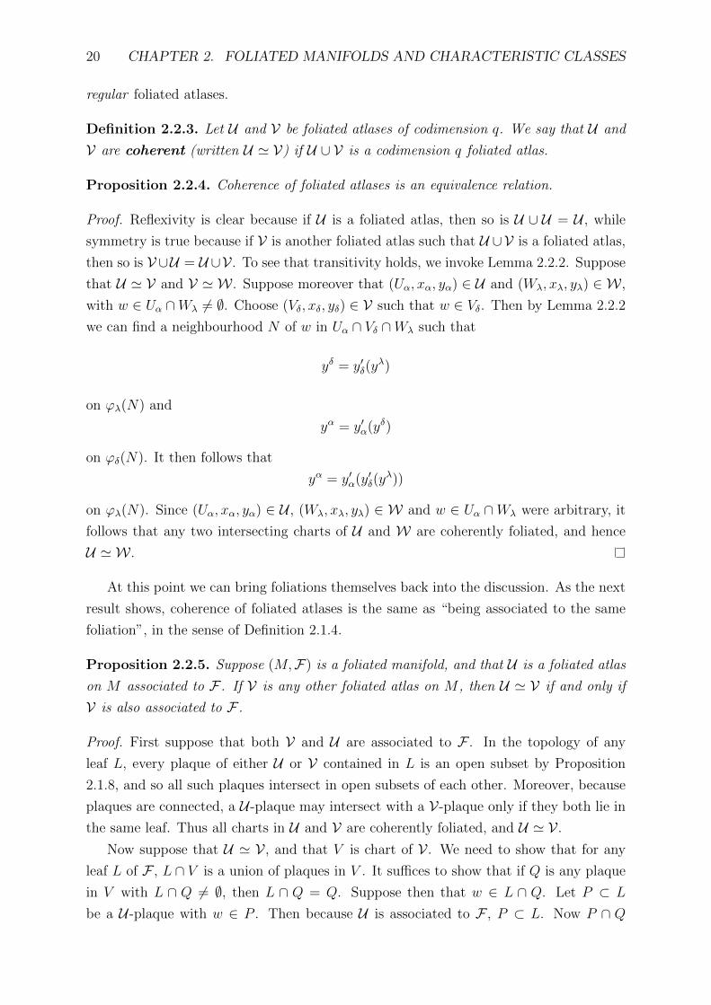
Definition 2.2.3. Let U and V be foliated atlases of codimension q. We say that U and
V are coherent (written U ' V) if U ∪ V is a codimension q foliated atlas.
Proposition 2.2.4. Coherence of foliated atlases is an equivalence relation.
Proof. Reflexivity is clear because if U is a foliated atlas, then so is U ∪ U = U , while
symmetry is true because if V is another foliated atlas such that U ∪V is a foliated atlas,
then so is V ∪U = U ∪V . To see that transitivity holds, we invoke Lemma 2.2.2. Suppose
that U ' V and V ' W . Suppose moreover that (Uα, xα, yα) ∈ U and (Wλ, xλ, yλ) ∈ W ,
with w ∈ Uα ∩Wλ 6= ∅. Choose (Vδ, xδ, yδ) ∈ V such that w ∈ Vδ. Then by Lemma 2.2.2
we can find a neighbourhood N of w in Uα ∩ Vδ ∩Wλ such that
yδ = y′δ(yλ)
on ϕλ(N) and
yα = y′α(yδ)
on ϕδ(N). It then follows that
yα = y′α(y′δ(yλ))
on ϕλ(N). Since (Uα, xα, yα) ∈ U , (Wλ, xλ, yλ) ∈ W and w ∈ Uα ∩Wλ were arbitrary, it
follows that any two intersecting charts of U and W are coherently foliated, and hence
U ' W .
At this point we can bring foliations themselves back into the discussion. As the next
result shows, coherence of foliated atlases is the same as “being associated to the same
foliation”, in the sense of Definition 2.1.4.
Proposition 2.2.5. Suppose (M,F) is a foliated manifold, and that U is a foliated atlas
on M associated to F . If V is any other foliated atlas on M , then U ' V if and only if
V is also associated to F .
Proof. First suppose that both V and U are associated to F . In the topology of any
leaf L, every plaque of either U or V contained in L is an open subset by Proposition
2.1.8, and so all such plaques intersect in open subsets of each other. Moreover, because
plaques are connected, a U -plaque may intersect with a V-plaque only if they both lie in
the same leaf. Thus all charts in U and V are coherently foliated, and U ' V .
Now suppose that U ' V , and that V is chart of V . We need to show that for any
leaf L of F , L ∩ V is a union of plaques in V . It suffices to show that if Q is any plaque
in V with L ∩ Q 6= ∅, then L ∩ Q = Q. Suppose then that w ∈ L ∩ Q. Let P ⊂ L
be a U -plaque with w ∈ P . Then because U is associated to F , P ⊂ L. Now P ∩ Q

2.2. THE LOCAL STRUCTURE OF A FOLIATED MANIFOLD 21
is nonempty since it must contain w, and since U ' V , P ∩ Q is open in Q. Moreover,
because P ∩Q ⊂ L∩Q and w is arbitrary, it follows that L∩Q is open in Q. Thus Q is
the union of disjoint open subsets, each of which is the intersection of Q with some leaf
of F . Connectedness of Q then forces L ∩Q = Q, as required.
Proposition 2.2.5 gives us some freedom to choose well-behaved atlases when studying
a foliation. Observe that a foliated atlas in the sense of Definition 2.2.1 allows for some
quite nasty behaviour in at least one crucial way - namely, there is nothing preventing
a plaque of one foliated chart from intersecting infinitely many plaques of another foli-
ated chart. Ultimately, holonomy will be defined by drawing paths through intersecting
plaques in neighbouring foliated charts: if our charts aren’t small enough that any given
plaque intersects at most one plaque from any neighbouring foliated chart, then it will be
impossible to define holonomy in this manner. Thankfully, coherence is a weak enough
equivalence relation that choosing a foliated atlas of sufficiently small charts is always
possible.
Definition 2.2.6. A foliated atlas U = (Uα, ϕα)α∈A of codimension q on a manifold
M is said to be regular if
1. for each α ∈ A, there is a foliated chart (Wα, ψα) on M that is associated to F but
not necessarily itself an element of U , such that Uα is a compact subset of Wα and
ϕα = ψα|Uα;
2. the cover Uαα∈A is locally finite, hence, by second countability of M , countable,
and;
3. if (Uα, ϕα), (Uβ, ϕβ) ∈ U , then the interior of each closed plaque P ⊂ Uα meets at
most one plaque in Uβ.
Property (1) in Definition 2.2.6 means that the homeomorphism ϕα = (xα, yα) between
Uα and Bτ ×Bt extends canonically to homeomorphism ϕα = (xα, yα) of the closure Uα
of Uα with Bτ × Bt. Enforcing property (3) in Definition 2.2.6 guarantees precisely the
intersection property of plaques required to define holonomy. Lemma 2.2.7 should be
thought of as a global version of the analogous Lemma 2.2.2, and will provide us with
formulae with which to define holonomy.
Lemma 2.2.7. Let U be a foliated atlas on an n-manifold M satisfying property (1) of
Definition 2.2.6. Then U satisfies property (3) of Definition 2.2.6 if and only if whenever
Uα ∩ Uβ 6= ∅, the transverse coordinate change yα = y′α(xβ, yβ) is independent of xβ on
all of ϕβ(Uα ∩ Uβ).
Proof. First suppose that U satisfies property (3), and suppose that Uα ∩ Uβ 6= ∅. Then
Uα ∩ Uβ 6= ∅, and every closed plaque P ⊂ Uβ with P ∩ Uα 6= ∅ has interior meeting at

22 CHAPTER 2. FOLIATED MANIFOLDS AND CHARACTERISTIC CLASSES
most one plaque of Uα. Suppose that P = P yβ = ϕ−1β (B
β
τ ×yβ), with yβ ∈ yβ(Uα∩Uβ)
so that yβ is identically equal to yβ on P . Suppose that the interior P of P meets the
plaque P yα = ϕ−1α (B
α
τ ×yα) for some yα ∈ yα(Uα∩Uβ). Then for any xβ ∈ xβ(P∩P yα),
we can find xα ∈ xα(P ∩ P yα) such that ϕ−1β (xβ, yβ) = ϕ−1
α (xα, yα), and we have
y′α(xβ, yβ) = yα(ϕ−1β (xβ, yβ)) = yα(ϕ−1
α (xα, yα)) = yα.
By continuity of y′α, we in fact have that
y′α(xβ, yβ) = yα
for all xβ ∈ xβ(P ∩ P yα). Because yβ was arbitrary, we conclude that the transverse
change of coordinates yα = y′α(yβ) is independent of xβ as claimed.
Now suppose that yα = y′α(yβ) is independent of xβ on ϕβ(Uα ∩ Uβ). If P is a closed
plaque in Uβ which has empty intersection with Uα, then P will meet no plaques in Uα.
On the other hand, suppose that yβ ∈ yβ(Uα ∩ Uβ) and that P = P yβ . If the interior P
of P intersects Uα in two distinct plaques P yα1and P yα2
, we can find distinct xβ1 , xβ2 ∈ Bβ
τ
such that
ϕ−1β (xβ1 , y
β) ∈ P ∩ P yα1and ϕ−1
β (xβ2 , yβ) ∈ P ∩ P yα2
.
But it then follows that
y′α(xβ1 , yβ) = yα1 6= yα2 = y′α(xβ2 , y
β),
contradicting the hypothesis that y′α is independent of xβ. Since P was arbitrary, we have
recovered (3).
Given a regular foliated atlas (Uα, ϕα)α∈A, Lemma 2.2.7 in particular guarantees
that the transverse coordinate change
yα = y′α(yβ)
is independent of xβ for all (xβ, yβ) ∈ ϕβ(Uα ∩ Uβ). Observe that for α, β ∈ A, we can
define a map cαβ : yβ(Uα ∩ Uβ)→ yα(Uα ∩ Uβ) by
cαβ(yβ) := y′α(yβ) = yα.
This cαβ is smooth as a map between open subsets of Rq because y′α is, and is bijective
because the foliated atlas is regular. Moreover it has a smooth inverse cβα, so is a
diffeomorphism. We note that on yδ(Uδ ∩ Uβ ∩ Uα) we have
cαδ = cαβ cβδ. (2.1)

2.2. THE LOCAL STRUCTURE OF A FOLIATED MANIFOLD 23
Definition 2.2.8. Let U = (Uα, ϕα)α∈A be a regular foliated atlas for an n-manifold
M . The collection c = cαβα,β∈A is called the holonomy cocycle of U and the formula
(2.1) is called the cocycle condition.
The holonomy cocycle of a regular foliated atlas associated to a foliation F keeps track
of how the leaves of F “move” relative to each other, provided they are sufficiently close
together, and provides our first glimpse at what sort of information holonomy encodes. It
can be shown [123, Page 9] that any family satisfying Equation (2.1) defined with respect
to some open cover of a manifold M defines a unique foliation of M .
We finally come to the main result of this section, which says that in studying foliations
we can always assume the existence of a regular foliated atlas.
Proposition 2.2.9. Every foliated atlas has a coherent refinement that is regular.
Proof. Fix a metric on M and a foliated atlas W for M . First suppose that M is
compact, and assume without loss of generality that W = (Wi, ψi)li=1 is finite. By
Lebesgue’s number lemma [135, Lemma 27.5], we can find ε > 0 such that any X ⊂ M
with diam(X) < ε is contained entirely in some Wi. For each x ∈M , choose i such that
x ∈ Wi, and choose an open neighbourhood U ′x of x such that U′x ⊂ Wi is compact in
Wi and for which diam(U ′x) < ε/2. Define ϕx := ψi|U ′x . Then (U ′x, ϕx) is a foliated chart
about x.
Now suppose that U ′x is contained in some Wk, for k 6= i. Write ψk = (xk, yk), so that
yk restricts to a submersion of U ′x into Rq. By Lemma 2.2.2, the point ϕx(x) ∈ ϕx(U ′x)has a neighbourhood Vx on which y′k : ϕx(U
′x) → Rq is locally constant in xi, and so we
can choose Ux ⊂ ϕ−1x (Vx) to be small enough that yk|Ux has the plaques of Ux as its level
sets. Thus each plaque of Wk contains at most one closed plaque of Ux. Repeating this
process for every member of the finite atlas W , we can ensure that whenever Ux ⊂ Wj,
distinct plaques of Ux lie in distinct plaques of Wj.
Now pass to a finite subatlas U = (Ui, ϕi)mi=1 of (Ux, ϕx)x∈M . If Ui ∩Uj 6= ∅, then
diam(Ui ∪ Uj) < ε, and so there is some number k such that U i ∪ U j ⊂ Wk. Distinct
plaques of U i lie in distinct plaques of Wk, and distinct plaques of U j lie in distinct
plaques of Wk also. Thus each plaque of U i has interior meeting at most one plaque of U j
and vice versa, so U is a regular foliated atlas. Moreover, U is coherent with W because
plaques of U are always contained as open subsets of plaques of W .
We now turn to the case where M is not compact. Since M is locally compact and
second countable, we can choose a sequence Ki∞i=0 of compact subsets of M such that
Ki ⊂ Ki+1 for all i ≥ 0 (the here denotes “interior”), and such that
M =∞⋃i=0
Ki.

24 CHAPTER 2. FOLIATED MANIFOLDS AND CHARACTERISTIC CLASSES
Since M is second countable, we may assume without loss of generality that W =
(Wi, ψi)∞i=0 is countable. We can then choose a strictly increasing sequence nl∞l=0
of positive integers such that
Wl = (Wi, ψi)nli=0
covers Kl. For each l, define
δl := infx∈Kl,y∈∂Kl+1
d(x, y),
where d denotes the metric on M . For each l, choose εl > 0 such that
εl < minδl/2, εl−1
for l ≥ 1, with ε0 < δ0/2. Insist furthermore, using the Lebesgue number lemma, that
if X ⊂ M meets Kl (respectively Kl+1) and diam(X) < εl, then X is contained in some
element of the open cover Wl of the compact space Kl (respectively the open cover Wl+1
of the compact space Kl+1). For each x ∈ Kl \Kl−1, construct (Ux, ϕx) as in the compact
case, with Ux a compact subset of some Wj, diam(Ux) < εl/2 and ϕx = ψj|Ux , and such
that whenever Ux ⊂ Wk for k 6= j, the plaques of Ux are contained in distinct plaques of
Wk. As with the compact case, pass to a finite subcover (Ui, ϕi)nli=nl−1+1 of Kl \Kl−1
(taking n−1 = 0). We then obtain a regular foliated atlas U = (Ui, ϕi)∞i=1 that refines
W and is coherent with W .
2.3 The classical Godbillon-Vey invariant
With a basic knowledge of foliated charts for foliated manifolds, one is able to construct
the Godbillon-Vey invariant of any transversely orientable (defined below) foliated man-
ifold. The construction we give here is an adaptation of the original construction given
by Godbillon and Vey for codimension 1 foliations [81] to foliations of arbitrary codi-
mension. We will also give the calculation due to Roussarie in [81] of the Godbillon-Vey
invariant of the Roussarie foliation (Example 2.1.7), exhibiting a foliated manifold whose
Godbillon-Vey invariant is nonzero.
Later we will see how the Godbillon-Vey invariant can be accessed using an adaptation
of Chern-Weil theory enabled by Bott’s vanishing theorem [22], and, in the final chapters,
using the techniques of groupoid cohomology and noncommutative geometry.
Definition 2.3.1. Associated to any foliated manifold (M,F) is its leafwise tangent
bundle T F ⊂ TM consisting of all tangents to leaves, and its normal bundle N :=
TM/T F . A foliation (M,F) is said to be transversely orientable if its normal bundle
N = TM/T F is orientable as a vector bundle: that is if there exists a nonvanishing
section ω of Λq(N∗).

2.3. THE CLASSICAL GODBILLON-VEY INVARIANT 25
The dual N∗ → T ∗M of the projection TM → N permits us to make an identification
of the orientation form ω ∈ Γ∞(M ; Λq(N∗)) of N with a nonvanishing q-form ω ∈ Ωq(M)
for which
ω(X1 ∧ · · · ∧Xq) = 0
whenever any one of the Xi is an element of Γ∞(M ;T F).
Definition 2.3.2. Let (M,F) be a foliated manifold of codimension q. A differential
k-form ω on M is said to be a transverse differential form if
ω(X1 ∧ · · · ∧Xk) = 0
whenever any one of the Xi ∈ Γ∞(M ;T F). If moreover (M,F) is transversely orientable,
a nonvanishing, transverse differential q-form is called a transverse volume form and
is said to define the foliation F .
Remark 2.3.3. A transverse differential k-form ω naturally defines a k-form ω on the
normal bundle N . More specifically, letting p : TM → N denote the projection, the
formula
ω(pX1 ∧ · · · ∧ pXk) := ω(X1 ∧ · · · ∧Xk), X1, . . . , Xk ∈ Γ∞(M ;TM)
is well-defined since ω vanishes whenever any one of its inputs is a leafwise tangent
field. Conversely, if ω ∈ Γ∞(M ; ΛkN∗) is any k-form on N , then we obtain a transverse
differential k-form ω on M by defining
ω(X1 ∧ · · · ∧Xk) := ω(pX1 ∧ · · · ∧ pXk), X1, . . . , Xk ∈ Γ∞(M ;TM).
Thus transverse differential forms are in one to one correspondence with exterior forms
on N .
Notice that the collection of transverse differential forms are not in general closed un-
der the exterior derivative. This is essentially due to the fact that even while a transverse
differential form annihilates leafwise vectors, it may still vary along leaves. Consequently
the transverse differential forms cannot in general be formed into a complex. By con-
sidering the subspace of transverse forms that are also locally constant along leaves (the
basic forms), one does obtain a complex known as the basic complex [146].
Remark 2.3.4. Our nomenclature here is not to be confused with that of A. Haefliger
[91, p. 51], for whom a transverse volume form must satisfy the additional requirement of
being closed as a differential form. Note that any transverse volume form in the sense of
Definition 2.3.2 which is locally constant along leaves is, by dimension count, a transverse
volume form in the sense Haefliger.

26 CHAPTER 2. FOLIATED MANIFOLDS AND CHARACTERISTIC CLASSES
Let us now assume that we have a transversely orientable foliated manifold (M,F)
of codimension q, and that ω ∈ Ωq(M) is a transverse volume form for F . Furthermore
let U = (Uα, ϕα = (xα, zα))α∈A be an atlas of foliated charts for (M,F), and denote
the leaf dimension of F by p. Then for each α ∈ A there exists a nonvanishing function
fα ∈ C∞(Uα) such that ωα := ω|Uα = fαdz1α ∧ · · · ∧ dzqα. We calculate
dωα = dfα ∧ dz1α ∧ · · · ∧ dzqα =
1
fαdfα ∧ ωα = d(log |fα|) ∧ ωα,
where we have used the fact that fα is nonvanishing in the second equality. Now taking
a partition of unity (λα)α∈A we see that η :=∑
α λαd(log |fα|) ∈ Ω1(M) satisfies
dω =∑α
λαdωα =∑α
λαd(log |fα|) ∧ ωα =∑α
λαd(log |fα|) ∧ ω = η ∧ ω.
We now consider the differential form η ∧ (dη)q.
Theorem 2.3.5. Let (M,F) be a transversely orientable foliated manifold of codimension
q, let ω ∈ Ωq(M) be a transverse volume form and let η ∈ Ω1(M) be such that dω = η∧ω.
Then the 2q + 1-form η ∧ (dη)q is closed, and its class in H2q+1dR (M,R) is independent of
the choices of ω and η.
Proof. That dω = η ∧ ω implies that
0 = d2ω = d(η ∧ ω) = dη ∧ ω − η ∧ dω = dη ∧ ω − η ∧ η ∧ ω = dη ∧ ω. (2.2)
Since ω is a nowhere vanishing transverse q-form, in any foliated chart (U, (x, z)), ω is a
nonzero C∞(U)-multiple of dz1 ∧ · · · ∧ dzq. Therefore Equation (2.2) implies that dη has
the form
dη =
p∑i=1
q∑j=1
fijdxi ∧ dzj
on U . Consequently, on U , (dη)q+1 is a sum of terms of the form
fI,JdxI ∧ dzJ ,
where |J | = q + 1 > q, hence must be identically zero. Thus
d(η ∧ (dη)q) = (dη)q+1 = 0,
and η ∧ (dη)q is closed.
Now suppose that η′ ∈ Ω1(M) is another form such that dω = η′ ∧ ω. Then we see
that (η′ − η) ∧ ω = 0. Thus, by the nonsingularity of ω, in any foliated chart (U, (x, z))

2.3. THE CLASSICAL GODBILLON-VEY INVARIANT 27
there exist βi ∈ C∞(U) so that β := η′ − η takes the form
β =
q∑i=1
βidzi.
Consider now
η′ ∧ (dη′)q = (β + η) ∧ (dβ + dη)q = β ∧ (dβ + dη)q + η ∧ (dβ + dη)q.
The first summand here is necessarily zero because it will contain terms of the form
dxI ∧ dzJ with |J | > q. In the second summand, since both dβ and dη are of degree 2 we
have constants aj such that
(dβ + dη)q =
q∑j=0
aj(dβ)j ∧ (dη)q−j = (dη)q +
q∑j=1
aj(dβ)j ∧ (dη)q−j
=(dη)q + dβ ∧q∑j=1
aj(dβ)j−1 ∧ (dη)q−j = (dη)q + dβ ∧ γ,
where dγ = 0. We can now write
η′∧(dη′)q = η∧(dη)q+η∧dβ∧γ = η∧(dη)q+η∧d(β∧γ) = η∧(dη)q−d(η∧β∧γ)+dη∧β∧γ.
Now, over any chart (U, (x, z)), γ consists of terms of the form γI,JdxI ∧ dzJ where
|J | = q − 1, hence dη ∧ β ∧ γ = 0. Thus
η′ ∧ (dη′)q = η ∧ (dη)q − d(η ∧ β ∧ γ)
giving [η′ ∧ (dη′)q] = [η ∧ (dη)q] ∈ H2q+1dR (M).
Finally suppose that ω′ = fω for some nonvanishing function f ∈ C∞(M). Then
dω′ = d(fω) = df ∧ ω + fdω = df ∧ ω + fη ∧ ω = (d(log |f |) + η) ∧ ω′ = η′′ ∧ ω′.
Then we have dη′′ = dη, hence
η′′ ∧ (dη′′)q = (d(log |f |) + η) ∧ (dη)q = η ∧ (dη)q + d(log |f |(dη)q)
giving [η′′ ∧ (dη′′)q] = [η ∧ (dη)q] in H2q+1dR (M).
A-priori there is no reason to assume that the Godbillon-Vey invariant of any foliated
manifold is nontrivial. We now show, as in [81], that for the Roussarie foliation of
Example 2.1.7 the Godbillon-Vey invariant is a multiple of the fundamental class in de
Rham cohomology so is nonzero.
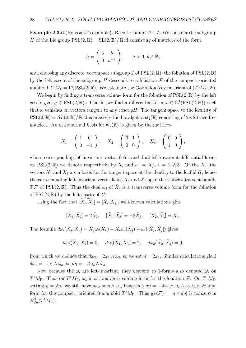
28 CHAPTER 2. FOLIATED MANIFOLDS AND CHARACTERISTIC CLASSES
Example 2.3.6 (Roussarie’s example). Recall Example 2.1.7. We consider the subgroup
H of the Lie group PSL(2,R) = SL(2,R)/R id consisting of matrices of the form
h =
(a b
0 a−1
), a > 0, b ∈ R,
and, choosing any discrete, cocompact subgroup Γ of PSL(2,R), the foliation of PSL(2,R)
by the left cosets of the subgroup H descends to a foliation F of the compact, oriented
manifold T 1MΓ = Γ\PSL(2,R). We calculate the Godbillon-Vey invariant of (T 1MΓ,F).
We begin by finding a transverse volume form for the foliation of PSL(2,R) by the left
cosets gH, g ∈ PSL(2,R). That is, we find a differential form ω ∈ Ω1(PSL(2,R)) such
that ω vanishes on vectors tangent to any coset gH. The tangent space to the identity of
PSL(2,R) = SL(2,R)/R id is precisely the Lie algebra sl2(R) consisting of 2×2 trace-free
matrices. An orthonormal basis for sl2(R) is given by the matrices
X1 =
(1 0
0 −1
), X2 =
(0 1
0 0
), X3 =
(0 0
1 0
),
whose corresponding left-invariant vector fields and dual left-invariant differential forms
on PSL(2,R) we denote respectively by Xi and ωi = X∗i , i = 1, 2, 3. Of the Xi, the
vectors X1 and X2 are a basis for the tangent space at the identity to the leaf idH, hence
the corresponding left-invariant vector fields X1 and X2 span the leafwise tangent bundle
T F of PSL(2,R). Thus the dual ω3 of X3 is a transverse volume form for the foliation
of PSL(2,R) by the left cosets of H.
Using the fact that ˜[Xi, Xj] = [Xi, Xj], well-known calculations give
[X1, X2] = 2X2, [X1, X3] = −2X3, [X2, X3] = X1.
The formula dωi(Xj, Xk) = Xjωi(Xk)− Xkωi(Xj)− ωi([Xj, Xj]) gives
dω3(X1, X2) = 0, dω3(X1, X3) = 2, dω3(X2, X3) = 0,
from which we deduce that dω3 = 2ω1 ∧ ω3, so we set η = 2ω1. Similar calculations yield
dω1 = −ω2 ∧ ω3, so dη = −2ω2 ∧ ω3.
Now because the ωi are left-invariant, they descend to 1-forms also denoted ωi on
T 1MΓ. Thus on T 1MΓ, ω3 is a transverse volume form for the foliation F . On T 1MΓ,
setting η = 2ω1 we still have dω3 = η ∧ ω3, hence η ∧ dη = −4ω1 ∧ ω2 ∧ ω3 is a volume
form for the compact, oriented 3-manifold T 1MΓ. Thus gv(F) = [η ∧ dη] is nonzero in
H3dR(T 1MΓ).

2.4. CHERN-WEIL THEORY AND SECONDARY CHARACTERISTIC CLASSES 29
Let us remark that in Example 2.3.6, the volume form η∧dη on T 1MΓ that represents
gv(F) can of course be integrated over T 1MΓ to give a number called the Godbillon-Vey
number, which is precisely the pairing of gv(F) with the fundamental class of M . That
a Godbillon-Vey number can be produced in this fashion is true of any codimension 1
foliation of any 3-manifold, and it is a celebrated result of Thurston [148] that for each
real number t ∈ R, there is a foliation F t of the 3-sphere S3 whose Godbillon-Vey number
is t. Thurston has also extended this result to higher codimension [149], constructing a
family of codimension q foliations whose Godbillon-Vey invariants surject onto the real
line. The Godbillon-Vey invariant is therefore far from trivial.
2.4 Chern-Weil theory and secondary characteristic
classes
We begin this section by recalling the Chern-Weil theory for connections on real vector
bundles. Most of the arguments presented in this section are adapted from the lecture
notes [128], which is a particularly efficient take on [125, Chapter 5], [23] and [35, Chapter
5].
2.4.1 Chern-Weil theory for vector bundles
It is an amazing fact due to S. S. Chern and A. Weil [49] that the curvatures of connec-
tions on vector bundles give us access to very concrete classes in de Rham cohomology.
The simplest examples of these classes are obtained by “tracing out” the endomorphism
component of the endomorphism-valued 2-form that is the curvature of a connection,
leaving only a differential form on the manifold. More generally, one obtains a differen-
tial form from the curvature of a connection by applying an invariant polynomial to the
curvature .
Definition 2.4.1. Let gl(r,R) = Mr(R) denote the Lie algebra of the matrix group
GL(r,R), consisting of all r × r real matrices. A map p : gl(r,R) → R is said to be an
invariant polynomial if for all A ∈ gl(r,R), p(A) is a polynomial in the entries of A,
and if for any g ∈ GL(r,R) one has p(gAg−1) = p(A).
Proposition 2.4.2. Let E be a real vector bundle over a manifold M . For any ω ∈Ωk(M,End(E)) and any invariant polynomial p : gl(r,R) → R homogeneous of degree
deg(p), there is a differential form p(ω) ∈ Ωk·deg(p)(M) obtained by applying p to ω in any
local trivialisation
Proof. In any local trivialisation U for E, we have End(E)|U ∼= U ×Mn(R), and under
this identification we can write ω|U = (ωij)ri,j=1 as an r × r matrix of k-forms. We can
then apply p to the matrix ω|U to obtain a k · deg(p)-form p(ω|U) ∈ Ωk·deg(p)(U).

30 CHAPTER 2. FOLIATED MANIFOLDS AND CHARACTERISTIC CLASSES
If V is any trivialisation that overlaps with U , then the corresponding transition
function ϕU,V : (U ∩ V ) ×Mn(R) → (U ∩ V ) ×Mn(R) is precisely conjugation in the
Mn(R) fibres by some GL(r,R)-valued function AU,V on U ∩ V . On U ∩ V we then have
that
p(ω|U) = p(AU,V ω|VA−1U,V ) = p(ω|V )
by invariance of p, so the local forms p(ω|U) assemble to a globally defined k-form p(ω) ∈Ωk·deg(p)(M).
Before we proceed any further let us pause to outline the algebraic structure at play
here. First observe that sums, products and scalar multiples of any two invariant poly-
nomials on gl(r,R) are again invariant under conjugation by invertible matrices. Thus
the collection of all such invariant polynomials forms an algebra, denoted I∗r (R). The
reasoning for the ∗-notation is as a placeholder for a specific grading that will make the
relationship with de Rham cohomology much cleaner.
Definition 2.4.3. For k ∈ N, define I2kr (R) to be the invariant polynomials on gl(r,R)
of degree k, and define I2k−1r (R) to be zero. Then I∗r (R) =
⊕n∈N I
nr (R) is the graded
algebra of invariant polynomials on gl(r,R).
It will simplify matters later to use a particular set of generators of the algebra
I∗r (R). Consider the trace Tr : Mn(R) → R. The trace is invariant under conjugation
by invertible matrices, so defines an element p1 ∈ I2r (R). Because the trace is invariant
under conjugation, so too is the polynomial
pk(A) := Tr(Ak),
which defines pk ∈ I2kr (R). It can be shown [35, Lemma 5.2.6] that I∗r (R) is generated as
a real graded algebra by p1, . . . , pr. Thus we make the identification
I∗r (R) = R[p1, . . . , pr]
of graded algebras.
Theorem 2.4.4 (Chern-Weil). Let ∇ be a connection on E with curvature R. Then for
any k ∈ N we have:
1. the differential form pk(R) is closed, and so defines a class in H2kdR(M); and
2. if ∇′ is any other connection on E, with curvature R′ and with α = ∇ − ∇′ ∈Ω1(M,End(E)), then
pk(R)− pk(R′) = d(k
∫ 1
0
Tr(α ∧Rk−1t )dt
),

2.4. CHERN-WEIL THEORY AND SECONDARY CHARACTERISTIC CLASSES 31
where Rt denotes the curvature of the connection ∇t = (1− t)∇′ + t∇.
Thus the connection ∇ on E determines a homomorphism φE,∇ : I∗r (R) → H∗dR(M) of
graded algebras, and this homomorphism is independent of the connection chosen.
To prove Theorem 2.4.4, we need the following short lemma.
Lemma 2.4.5. Let ∇ be a connection on E. Then for any A ∈ Ωk(M,End(E)) we have
dTr(A) = Tr([∇, A])
Proof. Over any sufficiently small open set U in M , by Lemma C.0.2 we have ∇ = d+α
for some α ∈ Ω1(U, gl(r,R)), while any A ∈ Ωk(M,End(E)) can be regarded as an r × rmatrix of differential k-forms on U . For any such A we have
[∇, A] = [d+ α,A] = dA+ [α,A].
Since the matrix trace vanishes on commutators of matrices we get
Tr([∇, A]) = dTr(A),
independent of U .
Proof of Theorem 2.4.4. Fix k ∈ N. By Lemma 2.4.5 we have
d(pk(R)) = dTr(Rk) = Tr([∇, Rk]) = Tr([∇,∇2k]) = 0,
so pk(R) is indeed a closed differential form.
For the second part, the fundamental theorem of calculus tells us that
pk(R)− pk(R′) =
∫ 1
0
d
dtTr(Rk
t )dt,
so it suffices to show that ddt
Tr(Rkt ) is of the desired form. We calculate
d
dtTr(Rk
t ) = Tr(d
dtRkt ) = kTr
(( ddtRt
)Rk−1t
)= kTr
(( ddt∇2t
)∇2(k−1)t
)=kTr
((( ddt∇t
)∇t +∇t
( ddt∇t
))∇2(k−1)t
)= kTr
((α∇t +∇tα
)∇2(k−1)t
)=kTr
([∇t, α∇2(k−1)
t ])
= kTr(d(α ∧Rk−1
t ))
= kdTr(α ∧Rk−1t ),
where we have used Lemma 2.4.5 for the third-from-last equality, and so
pk(R)− pk(R′) = d(k
∫ 1
0
Tr(α ∧Rk−1t )dt
)

32 CHAPTER 2. FOLIATED MANIFOLDS AND CHARACTERISTIC CLASSES
as claimed.
For the final claim, we define φ∇,E on any generator pk by φE,∇(pk) := [pk(E)]. Then
φ∇,E is by definition a homomorphism of graded algebras, and by (2) for any other choice
of connection ∇′, the homomorphisms φE,∇ and φE,∇′ agree.
Definition 2.4.6. The homomorphism φE : I∗r (R) → H∗dR(M) defined on generators pk
by
φE(pk) := [pk(R)],
where R is the curvature of any connection on E, is called the Chern-Weil homomor-
phism.
The image under φE of the algebra I∗r (R) is called the Pontryagin algebra of E,
denoted Pont(E), and the class φE(pk) = [pk(E)] determined by the generator pk is called
the kth Pontryagin class of E.
Observe that because of the grading with which we have equipped I∗r (R), the kth
Pontryagin class [pk(E)] of a vector bundle actually has degree 2k in H∗dR(M), just as
pk itself has degree 2k in I∗r (R). There is an immediate vanishing result for Pontryagin
classes coming from the notion of a metric connection, which tells us that only those
Pontryagin classes in degree 4k, k ∈ N, are nonzero.
Definition 2.4.7. Suppose that E is equipped with a Euclidean metric 〈·, ·〉. A connection
∇ on E is said to be metric compatible or a metric connection if for all X ∈Γ∞(M ;TM) we have
X〈σ1, σ2〉 = 〈∇Xσ1, σ2〉+ 〈σ1,∇Xσ2〉
for all σ1, σ2 ∈ Γ∞(M ;E). Here ∇Xσ is by definition ∇(σ)(X).
Proposition 2.4.8. Let k ∈ N be odd. Then for any metric connection ∇ on E with
curvature R, pk(R) = 0 in Ω2k(M), hence [pk(E)] = 0 in H2kdR(M).
Proof. Fix a Euclidean structure 〈·, ·〉 on E, and a metric connection ∇ for E. For any
tangent vector fields X and Y on M we will show that RX,Y is antisymmetric with respect
to the Euclidean structure. For smooth sections σ1, σ2 of E we calculate
XY 〈σ1, σ2〉 =X(〈∇Y σ1, σ2〉+ 〈σ1,∇Xσ2〉
)=〈∇X∇Y σ1, σ2〉+ 〈∇Y σ1,∇Xσ2〉+ 〈∇Xσ1,∇Y σ2〉+ 〈σ1,∇X∇Y σ2〉,
from which we deduce that
(XY − Y X)〈σ1, σ2〉 = 〈[∇X ,∇Y ]σ1, σ2〉+ 〈σ1, [∇X ,∇Y ]σ2〉,

2.4. CHERN-WEIL THEORY AND SECONDARY CHARACTERISTIC CLASSES 33
with the cross terms from XY 〈σ1, σ2〉 cancelling with those of Y X〈σ1, σ2〉. On the other
hand,
[X, Y ]〈σ1, σ2〉 = 〈∇[X,Y ]σ1, σ2〉+ 〈σ1,∇[X,Y ]σ2〉,
so (XY − Y X − [X, Y ]) = 0 gives us
〈([∇X ,∇Y ]−∇[X,Y ])σ1, σ2〉+ 〈σ1, ([∇X ,∇Y ]−∇[X,Y ])σ2〉 = 0,
which in light of Lemma C.0.7 means that RT = −R. Now, since k is odd we have
equalities
pk(R) = Tr(Rk) = Tr((RT )k) = −Tr(Rk) = −pk(R),
implying that pk(R) = 0, hence [pk(E)] = 0.
Proposition 2.4.8 will be crucially used together with Bott’s vanishing theorem for
foliated manifolds, from which all secondary characteristic classes of foliations are derived.
Before applying the Chern-Weil machinery to foliations, we must study more closely
the differential forms appearing in the second part of Theorem 2.4.4.
Definition 2.4.9. Let π : E →M be a real vector bundle of rank r and let pk ∈ I∗r (R) be
a generator. For any two connections ∇0, ∇1 on E, let α = ∇1 −∇0 ∈ Ω1(M,End(E))
and let Rt denote the curvature of the connection ∇t := (1− t)∇0 + t∇1, t ∈ [0, 1]. The
differential form
Tk(∇0,∇1) := k
∫ 1
0
Tr(α ∧Rk−1t )dt
is called the kth transgression form for the connections ∇0 and ∇1, and is said to
transgress pk(R1)−pk(R0) in the sense that dTk(∇0,∇1) = pk(R1)−pk(R0) by Theorem
2.4.4.
Now, if k ∈ N is odd, then by Proposition 2.4.8 we can choose ∇0 to be a metric
connection so that in fact
dTk(∇0,∇) = pk(R)
for any connection ∇ on E with curvature R. Fixing a metric connection ∇0 in this man-
ner allows us to define an algebraic structure that simultaneously encodes the Pontryagin
algebra as well as the differential forms that transgress the odd Pontryagin classes.
Definition 2.4.10. Let o = 2⌊r+1
2
⌋− 1 be the largest odd number less than or equal to r,
let Λ[h1, h3, . . . , ho] be the graded commutative algebra over R generated by the symbols hk,
deg(hk) = 2k−1 and let R[c1, . . . , cr] be the graded commutative algebra over R generated
by the symbols ck, deg(ck) = 2k. The Weil algebra is the graded tensor product
WOr := R[c1, . . . , cr] ⊗R Λ[h1, h3, . . . , ho].

34 CHAPTER 2. FOLIATED MANIFOLDS AND CHARACTERISTIC CLASSES
Equipped with the differential d : WOr → WOr defined by
dck = 0 for k = 1, . . . , r dhk = ck for k = 1, 3, . . . , 2⌊r + 1
2
⌋− 1,
the Weil algebra is a differential graded algebra.
Intuitively, the even degree generators ck of the Weil algebra encode the elements of
the Pontryagin ring, while the odd degree generators hk capture the transgression forms.
Let us observe that without any additional information on the generators ck, hk of the
Weil algebra, the even cohomology Hev(WOr) is generated by the classes [ck] while the
odd cohomology Hodd(WOr) is zero. Thus H∗(WOr) is isomorphic as a graded algebra
to I∗r (R) under the assignment
I2kr (R) 3 pk 7→ [ck] ∈ H2k(WOr).
We see then that the Chern-Weil homomorphism factors through the cohomology of the
Weil algebra in the following manner.
Proposition 2.4.11. Given any two connections ∇], ∇ on E, with R the curvature of
∇ and with ∇] metric compatible for some Euclidean structure on E, define φE,∇],∇ :
WOr → Ω∗(M) by
φE,∇],∇(ck) := pk(R) for k = 1, . . . , r,
φE,∇],∇(hk) := Tk(∇],∇) for k = 1, 3, . . . , 2⌊r + 1
2
⌋− 1.
Then φE,∇],∇ is a homomorphism of differential graded algebras, and descends therefore
to a homomorphism φE,∇],∇ : H∗(WOr)→ H∗dR(M) that is independent of choices of ∇]
and ∇, and agrees with the Chern-Weil map upon identification of H∗(WOr) with I∗r (R).
Remark 2.4.12. Note that because the cohomology of WOr is isomorphic as a graded
algebra to I∗r (R), Proposition 2.4.11 says nothing new at the cohomological level when
compared with Theorem 2.4.4. We will see however, that for a foliation F of M the
Weil algebra (or rather a quotient of it) is instrumental in capturing the topological
information implied by F , and at this point the extra information at the cochain level
provided by Proposition 2.4.11 becomes cohomologically important.
Proof of Proposition 2.4.11. For any k we have deg(pk(R)) = 2k = deg(ck), while for k
odd we have deg(Tk(∇],∇)) = 2k − 1 = deg(hk), so φE,∇],∇ is indeed a homomorphism
of graded algebras. To see that it commutes with the differential, we calculate
φE,∇],∇(dck) = φE,∇],∇(0) = 0 = dpk(R) = dφE,∇],∇(ck)

2.4. CHERN-WEIL THEORY AND SECONDARY CHARACTERISTIC CLASSES 35
for all k, while for k odd we have
φE,∇],∇(dhk) = φE,∇],∇(ck) = pk(R) = dTk(∇],∇) = dφE,∇],∇(hk).
Thus φE,∇],∇ is indeed a homomorphism of differential graded algebras and so induces a
homomorphism φE,∇],∇ of graded algebras H∗(WOr)→ H∗dR(M).
Let us now show that the induced map on cohomology does not depend on the choices
of connection. Thus suppose that ∇] is adapted to the Euclidean structure 〈·, ·〉1 on E,
and let ∇] be a connection adapted to some other Euclidean structure 〈·, ·〉0 on E. Let
∇ be any other connection on E, and consider the bundle proj∗M E over M × [0, 1],
where projM : M × [0, 1] → M is the projection onto the first factor. We then obtain a
connection ∇ on proj∗M E by defining ∇t = (1− t)∇+ t∇ for t ∈ [0, 1].
Since the space of all Euclidean metrics on E is a convex set, we can can take proj∗M E
to be equipped with the Euclidean metric 〈·, ·〉 which, over t ∈ [0, 1], has the form
(1−t)〈·, ·〉0+t〈·, ·〉1. Then the connection∇]defined over t ∈ [0, 1] by∇]
t := (1−t)∇]+t∇]
is a metric connection for the structure 〈·, ·〉 on proj∗M E. We now have a map φE,∇],∇ :
H∗(WOr) → H∗dR(M × [0, 1]) which restricts to φE,∇],∇ and φE,∇],∇ on M × 0 and
M × 1 respectively, so by the homotopy invariance of de Rham cohomology we have
φE,∇],∇ = φE,∇],∇ on cohomology.
Remark 2.4.13. The terminology “Weil algebra” applied to the algebra WOr is some-
what misleading. In fact Weil algebras are far more general objects: to any Lie group
G is associated the Weil algebra W (g) of its Lie algebra, which can be thought of as
a “classifying algebra” for connections on principal G-bundles. A detailed treatment of
Weil algebras in general can be found in Appendix D.2, and we urge the reader to be-
come comfortable with this material as it will be invoked frequently in this thesis. Of
particular interest to us is the Weil algebra W (gl(r,R)) associated to the general lin-
ear Lie algebra, along with its SO(r,R)-basic version W (gl(r,R), SO(r,R)). The algebra
W (gl(r,R), SO(r,R)) admits a canonical inclusion WOr → W (gl(r,R), SO(r,R)) that
captures, at the level of Lie algebras, all of the cocycle and transgression information of
WOr, and is studied in detail in the Appendix D.3. In particular Corollary D.3.6 tells us
that the inclusion WOr → W (gl(r,R), SO(r,R)) induces an isomorphism on cohomology,
so the terminological abuse employed in referring to WOr as the Weil algebra is justified.
2.4.2 Chern-Weil theory for foliations
This section follows the classic exposition in [23], and is also informed by the more recent
[35, Chapter 6]. Let us now consider a foliated manifold (M,F) of codimension q, with
leafwise tangent bundle T F ⊂ TM . Recall that the normal bundle of (M,F) is the
quotient N = TM/T F . The Chern-Weil theory for (M,F) is obtained by considering

36 CHAPTER 2. FOLIATED MANIFOLDS AND CHARACTERISTIC CLASSES
connections on the normal bundle N which are flat in the direction of the leaves.
Definition 2.4.14. Let p : TM → N denote the quotient map. The Bott partial
connection on N is the linear map ∇[ : Γ∞(M ;T F)⊗Γ∞(M ;N)→ Γ∞(M ;N) defined
by
∇[Xσ := p([X, Yσ]),
where X ∈ Γ∞(M ;T F), σ ∈ Γ∞(M ;N) and Yσ ∈ Γ∞(M ;TM) is such that p(Yσ) = σ.
First note that the formula in Definition 2.4.14 is well-defined; if Y ′σ were any other
vector field such that p(Y ′σ) = σ then Y ′σ = Z + Yσ for some Z ∈ Γ∞(M ;T F) hence
p([X, Y ′σ]) = p([X, Yσ] + [X,Z]) = p([X, Yσ])
because [X,Z] ∈ Γ∞(M ;T F) ∈ ker(p).
Furthermore it is easy to see that the Bott partial connection satisfies the Liebniz
rule: if f ∈ C∞(M) and X, σ, Yσ are as in Definition 2.4.14, then by the chain rule
∇[X(fσ) = p([X, fYσ]) = p(X(fYσ)−fYσX) = p(X(f)Yσ+f [X, Yσ]) = X(f)σ+f∇[
X(σ).
Thus the terminology “partial connection”, in reference to a linear map satisfying the
Liebniz rule for leafwise vector fields, makes sense. In order to apply the tools of Chern-
Weil theory to foliations, we will consider connections on N whose restriction to leafwise
vector fields is the Bott partial connection.
Definition 2.4.15. A connection ∇ on N for which ∇X = ∇[X for all X ∈ Γ∞(M ;T F)
is called a Bott connection and is said to be adapted to F .
Proposition 2.4.16. Bott connections on N exist.
Proof. Take a metric onM and consider any decomposition TM = T F ⊕N ′, so thatN ′ ∼=N . For any X ∈ Γ∞(M ;TM) let X = XT F +XN ′ be the corresponding decomposition.
For σ ∈ Γ∞(M ;N) and Yσ ∈ Γ∞(M ;TM) such that p(Yσ) = σ, define ∇ : Γ∞(M ;N)→Ω1(M,N) by
∇Xσ := ∇[XT F
σ + ∇XN′Yσ,
where ∇ is an arbitrary connection on N . Then ∇ satisfies the Liebniz rule because ∇[
and ∇ do, and is seen to be a Bott connection by taking X = XT F .
In what follows, we will use Bott connections instead of the Bott partial connection,
and so will denote any Bott connection by ∇[. What makes Bott connections such a
powerful tool for studying foliations is that they are flat along leaves.
Proposition 2.4.17. Let ∇[ be a Bott connection on N , and let R[ ∈ Ω2(M,End(N))
be its curvature form. Then R[X,Y = 0 for all X, Y ∈ Γ∞(M ;T F).

2.4. CHERN-WEIL THEORY AND SECONDARY CHARACTERISTIC CLASSES 37
Proof. For σ ∈ Γ∞(M ;N) and Yσ ∈ Γ∞(M ;TM) such that p(Yσ) = σ, we use Lemma
C.0.7 to calculate
R[X,Y σ = (∇[
X∇[Y −∇[
Y∇[X −∇[
[X,Y ])σ = p([X, [Y, Yσ]]− [Y, [X, Yσ]]− [[X, Y ], Yσ]) = 0
by the Jacobi identity.
That Bott connections are flat along leaves implies a vanishing of certain Pontryagin
classes of N by a simple counting of dimension, as first proved by R. Bott in [22].
Theorem 2.4.18 (Bott’s vanishing theorem). [22] All elements of the Pontryagin algebra
Pont(N) vanish in degree greater than 2q.
Proof. Take a Bott connection ∇[ on N . Since R[X,Y = 0 for all X, Y ∈ Γ∞(M ;T F), in
any foliated chart U the curvature R[ is of the form
R[ =
p∑i=1
q∑j=1
Rijdxi ∧ dzj +
q∑i,j=1
Rijdzi ∧ dzj.
where Rij, Rij ∈ Γ∞(M ; End(N)) and where (dxi)pi=1 and (dzi)qi=1 are differentials of the
plaque coordinates and transverse coordinates respectively in U . Raising this formula
to the power of k implies that each summand will contain dzi1 ∧ · · · ∧ dzik for some
i1, . . . , ik ⊂ 1, . . . , q, so k > q implies that each summand must be zero. Thus if
k > q and p ∈ I2kq (R) then p(R[) = 0.
Theorem 2.4.18 together with the proof of Proposition 2.4.8 have powerful implications
for the topology of M . Let ∇] be a fixed metric connection on N and let ∇[ be a Bott
connection on N , with curvatures R] and R[ respectively. Then
1. by Theorem 2.4.18, pk(R[) = 0 for all k > q,
2. by Proposition 2.4.8, pk(R]) = 0 for all odd k,
3. by Theorem 2.4.4, the transgression form Tk(∇],∇[) of Definition 2.4.9 satisfies
dTk(∇],∇[) = pk(R[)− pk(R])
for all k.
Thus if k > q is odd, then
dTk(∇],∇[) = pk(R[)− pk(R]) = 0.
That is, the transgression form Tk(∇],∇[) is closed, and so defines a class [Tk(∇],∇[)] in
H2k−1dR (M). We can summarise the existence of these new classes in the algebraic language
of Proposition 2.4.11 as follows.

38 CHAPTER 2. FOLIATED MANIFOLDS AND CHARACTERISTIC CLASSES
Definition 2.4.19. Let o be the largest odd number less than or equal to q and let
WOq = R[c1, . . . , cq] ⊗R Λ[h1, h3, . . . , ho]
be the Weil algebra. Let Iq denote the differential ideal of W generated by elements c⊗h,
c ∈ R[c1, . . . , cq], h ∈ Λ[h1, h3, . . . , ho], for which deg(c) > 2q. The truncated Weil
algebra is the differential graded algebra
WOq := WOq/Iq
obtained by taking the quotient. Using a mild abuse of notation, we will refer to the class
in WOq of any element a ∈ WOq by simply a.
Let us now consider an example to show that unlike the Weil algebra, the cohomology
of the truncated Weil algebra WOq is quite different from the graded algebra I∗q (R) of
invariant polynomials.
Example 2.4.20 (The Godbillon-Vey invariant in WOq). Consider the element gv :=
h1(c1)q of WOq. We calculate
d(h1(c1)q) = dh1(c1)q − h1d(c1)q = c1(c1)q = (c1)q+1 = 0,
using the facts that c1 is closed so d(c1)q = 0, and that (c1)q+1 has degree 2q + 2 so is
zero in WOq. It follows that [gv] = [h1(c1)q] ∈ H2q+1(WOq) is an odd cohomology class.
We refer to [gv] as the Godbillon-Vey class in WOq - we will see shortly that there is a
Chern-Weil-type homomorphism from H∗(WOq) into the de Rham cohomology of any
codimension q foliated manifold (M,F), and that under this homomorphism the class [gv]
is sent precisely to the class of the Godbillon-Vey invariant of (M,F). We have already
seen in Example 2.3.6 that there exist foliations with nonzero Godbillon-Vey invariant,
from which it follows that [gv] cannot be zero in H2q+1(WOq). This is in contrast to the
cohomology of the un-truncated Weil algebra, which is always zero in odd degree.
Theorem 2.4.21. [23, Proposition 10.13] Let ∇] be a metric connection on N and let ∇[
be a Bott connection on N . Then the homomorphism φN,∇],∇[ : WOq → Ω∗(M) descends
to a homomorphism φ∇],∇[ : WOq → Ω∗(M) of differential graded algebras. The induced
homomorphism φ∇],∇[ : H∗(WOq) → H∗dR(M) of graded algebras is independent of the
choices of ∇] and ∇[.
Proof. The first assertion follows from Theorem 2.4.18. The proof of Proposition 2.4.11
can be used to deduce the final statement once one observes that if ∇[0 and ∇[
1 are Bott
connections, then so too is ∇[t := (1− t)∇[
0 + t∇[1.

2.5. THE GODBILLON-VEY INVARIANT USING CHERN-WEIL THEORY 39
Definition 2.4.22. With ∇] a metric connection on N and with ∇[ a Bott connection
on N , the elements of the image of φ∇],∇[ that do not lie in the Pontryagin ring Pont(N)
of H∗dR(M) are called secondary or exotic characteristic classes for (M,F).
2.5 The Godbillon-Vey invariant using Chern-Weil
theory
For the entirety of this section we continue to denote by (M,F) a transversely orientable
foliated manifold of codimension q. Recall the construction for Theorem 2.3.5 of the
Godbillon-Vey of (M,F). One fixes a transverse volume form ω ∈ Ωq(M) and a 1-form
η ∈ Ωq(M) such that dω = η ∧ ω. Then the form η ∧ (dη)q is closed and its class in de
Rham cohomology is independent of the choices of η and ω.
We will now show that such differential forms η are closely related to Bott connections
on the normal bundle N . Using this fact, we will show that the Godbillon-Vey invariant
is the image under φ∇],∇[ of the element [h1(c1)q] ∈ H2q+1(WOq) for some choice of
connections ∇] and ∇[ as in Theorem 2.4.21. That this can be done in codimension 1 is
due to Bott [23, Lemma 10.4].
For higher codimension it is tempting to point to [35, p. 194] and [128, Proposition
3.5], however neither are complete arguments. More specifically, in [35] the result is
supposed to be a corollary of [35, Lemma 6.2.4], however this lemma concerns only
leafwise vector fields and therefore appears insufficient to establish the required result;
on the other hand the argument given in [128] is fundamentally local and does not easily
globalise. We give here what appears to be a novel approach which relies on the notion
of torsion for Bott connections.
Definition 2.5.1. Let ∇ be a connection on N , and let p : TM → N be the projection.
The torsion of the connection ∇ is the tensor T ∈ Γ∞(M ;T ∗M ⊗ T ∗M ⊗N) defined by
T (X, Y ) := ∇X(pY )−∇Y (pX)− p[X, Y ]
for all X, Y ∈ Γ∞(M ;TM). The connection ∇ is said to be torsion-free if T (X, Y ) = 0
for all X, Y ∈ Γ∞(M ;TM).
By taking F to be a foliation by points, one sees that Definition 2.5.1 generalises
the usual notion torsion for affine connections [65, 9.5.1]. In particular, taking ∇ to be
the Levi-Civita connection in the proof of Proposition 2.4.16, we see that we can assume
without loss of generality that Bott connections on N are torsion-free.
Proposition 2.5.2. Torsion-free Bott connections on N exist.

40 CHAPTER 2. FOLIATED MANIFOLDS AND CHARACTERISTIC CLASSES
Proof. As in the proof of Proposition 2.4.16, we take a Riemannian metric on M and
form the associated decomposition TM = T F ⊕N . For any X ∈ Γ∞(M ;TM) we let
X = XF +XN be the corresponding sum, and we define ∇[ on N by
∇[X(Y ) := [XF , Y ]N +∇LC
XNY,
where ∇LC is the Levi-Civita connection on M , whose torsion TLC is zero. We know
from Proposition 2.4.16 that ∇[ is a Bott connection. Moreover, for X, Y ∈ Γ∞(M ;TM)
we calculate
T (X, Y ) =∇[X(YN)−∇[
Y (XN)− [X, Y ]N
=([XF , YN ]N +∇LC
XNYN)−([YF , XN ]N +∇LC
YNXN
)− [XF +XN , YF + YN ]N
=[XF , YN ]N − [YF , XN ]N − [XF , YN ]N − [XN , YF ]N + TLC(XN , YN) = 0,
where we have used the fact that Γ∞(M ;T F) is closed under Lie brackets in going from
the second line to the third.
Torsion-free Bott connections are closely related to the exterior derivative on M . Let
us continue to assume that M is equipped with a Riemannian metric, with respect to
which N can be regarded as a subbundle of TM . Then for any torsion-free Bott connec-
tion ∇[ on N , let us abusively use the same notation to denote the induced connections
on the exterior powers ΛkN given for Z1, . . . , Zk ∈ Γ∞(M ;N) by
∇[X(Z1 ∧ · · · ∧ Zk) :=
k∑i=1
Z1 ∧ · · · ∧ ∇[XZi ∧ · · · ∧ Zk, X ∈ Γ∞(M ;TM),
and for the induced connections on Γ∞(M ; ΛkN∗) defined for ω ∈ Γ∞(M ; ΛkN∗) and
Z1, . . . , Zk ∈ Γ∞(M ;N) by
(∇[Xω)(Z1 ∧ · · · ∧ Zk) := X
(ω(Z1 ∧ · · · ∧ Zk)
)− ω
(∇[X(Z1 ∧ · · · ∧ Zk)
).
As in Remark 2.3.3, let p : TM → N denote the projection and let us identify elements
of Γ∞(M ; ΛkN∗) with the subspace of elements ω of Ωk(M) for which ω(X1∧ · · ·∧Xk) =
ω(pX1 ∧ · · · ∧ pXk) for all Xi ∈ Γ∞(M ;TM). Denote by Λ : Γ∞(M ;T ∗M ⊗ ΛkT ∗M)→Ωk+1(M) the antisymmetrisation map defined for η ⊗ ω ∈ Ω1(M)⊗ Ωk(M) by
Λ(η ⊗ ω)(X0 ∧ · · · ∧Xk) :=k∑i=0
(−1)iη(Xi)ω(X0 ∧ · · · ∧ Xi ∧ · · · ∧Xk)
for all X0, . . . , Xk ∈ Γ∞(M ;TM). We then have the following.

2.5. THE GODBILLON-VEY INVARIANT USING CHERN-WEIL THEORY 41
Proposition 2.5.3. Let ∇[ be a torsion-free Bott connection on N . Then the composition
Λ ∇[ coincides with the exterior derivative on the subspace Γ∞(M ; Λ∗N∗) of Ω∗(M).
Proof. Let p : TM → N be the projection, let ω ∈ Γ∞(M ; ΛkN∗), and let X0, . . . , Xk ∈Γ∞(M ;TM). For 0 ≤ i ≤ k we define
X∧i := X0 ∧ · · · ∧ Xi ∧ · · · ∧Xk,
and for i < j we define
X∧ij := X0 ∧ · · · ∧ Xi ∧ · · · ∧ Xj ∧ · · · ∧Xk,
where the · denotes omission. By abuse of notation, for each k we denote the induced
projection Λkp : ΛkTM → ΛkN by p as well. Then we calculate
(Λ ∇[
)ω(X0 ∧ · · · ∧Xk) =
k∑i=0
(−1)i(∇[Xiω)(X∧i )
=k∑i=0
(−1)iXi
(ω(pX∧i )
)−
k∑i=0
(−1)iω(∇[Xi
(pX∧i ))
=dω(X0 ∧ · · · ∧Xk)−∑i<j
(−1)i+jω(p[Xi, Xj] ∧ pX∧ij)
+∑i<j
(−1)i+jω((∇[
Xi(pXj)−∇[
Xj(pXi)) ∧ pX∧ij
)=dω(X0 ∧ · · · ∧Xk) +
∑i<j
(−1)i+jω(T (Xi, Xj) ∧ pX∧ij
)=dω(X0 ∧ · · · ∧Xk),
where we have used the fact that ∇[ is torsion-free in going from the fourth equality to
the last. Thus Λ ∇[ = d as required.
It is now easy to see that the Chern-Weil construction of the Godbillon-Vey invariant
agrees with the classical construction.
Theorem 2.5.4. Let ω ∈ Ωq(M) be a transverse volume form and let ∇[ be a torsion-free
Bott connection. Denoting the induced connection on ΛqN∗ by ∇[ also, if η ∈ Ω1(M) is
defined by the equation
∇[(fω) := (df + η)⊗ ω, f ∈ C∞(M), (2.3)
then dω = η ∧ ω. Moreover, letting R[ denote the curvature of ∇[, we have dη = Tr(R[).
Finally, if ∇] is any metric connection on N , we have φ∇],∇[(h1(c1)q) = η ∧ (dη)q,
hence φ∇],∇[([h1(c1)q]) = [η ∧ (dη)q] = gv ∈ H2q+1dR (M).

42 CHAPTER 2. FOLIATED MANIFOLDS AND CHARACTERISTIC CLASSES
Proof. Equation (2.3) defining η tells us in particular that ∇[ω = η⊗ω, so by Proposition
2.5.3 we have
dω = (Λ ∇[)ω = Λ(η ⊗ ω) = η ∧ ω.
Consider now an open set U in M , over which we have a local frame field ω = (ω1, . . . , ωq)
for N∗|U such that ω1∧· · ·∧ ωq = ω|U , and with respect to which the induced connection
on N∗|U has the form ∇[ = d+ α, where α ∈ Ω1(U ; gl(q,R)). Then over U , we have
∇[ω =∇[(ω1 ∧ · · · ∧ ωq) =
q∑i=1
ω1 ∧ · · · ∧ (α⊗ ω)i ∧ · · · ∧ ωq
=
q∑i,j=1
ω1 ∧ · · · ∧(αij ⊗ ωj
)∧ · · · ∧ ωq =
q∑i=1
αii ⊗(ω1 ∧ · · · ∧ ωq
)= tr(α)⊗ ω,
so by definition of η we have η|U = tr(α). Consequently, over U we see that
dη = d tr(α) = tr(dα) = tr(dα + α ∧ α) = tr(R[)
since the exterior product α∧ α is antisymmetric. Since M can be covered by such open
sets U we see that dη = tr(R[) globally.
Now let ∇] be a metric connection for N (inducing ∇] on N∗), and letting U and α
be as in the previous paragraph write ∇] = d + β over U , where α, β ∈ Ω1(U, gl(q,R)).
Since ∇] is a metric connection, β is antisymmetric so tr(β) = 0. Now
φ∇],∇[(h1) = T1(∇],∇[) =
∫ 1
0
tr(α− β)dt = tr(α) = η.
Moreover we have
φ∇],∇[(c1) = p1(R[) = tr(R[) = dη,
hence
φ∇],∇[(h1(c1)q) = η ∧ (dη)q
as claimed.
Let us remark that if (M,F) is a codimension q foliated manifold, then the Godbillon-
Vey invariant can be accessed whether (M,F) is transversely orientable or not [80, p.
156]. Indeed, Bott and metric connections can be found for the normal bundle N com-
pletely independently of any assumptions of transverse orientability, and Theorem 2.5.4
says that the more general Chern-Weil description using Bott and metric connections
agrees with the classical description for transversely orientable foliations. For the rest of
this thesis we will always assume transverse orientability.

Chapter 3
Holonomy and related constructions
3.1 Holonomy
Let (M,F) be a foliated manifold, and fix two points x, y ∈ M contained in the same
leaf L. Let γ be a path in L connecting x to y. If γ were contained in some plaque P
of a foliated chart, it would canonically determine a path γ in any neighbouring plaque
which one could follow from its source to its range. One might imagine more generally
that on any leaf L′ that is sufficiently close to L one could start at some point x′ in L′
near x, and “follow the path γ” on L′ so as to end up at some point y′ in L′ near y. This
is depicted in Figure 3.1 below.
Figure 3.1: “Following” the red path on L as we move along L′ takes us from x′ to y′
43
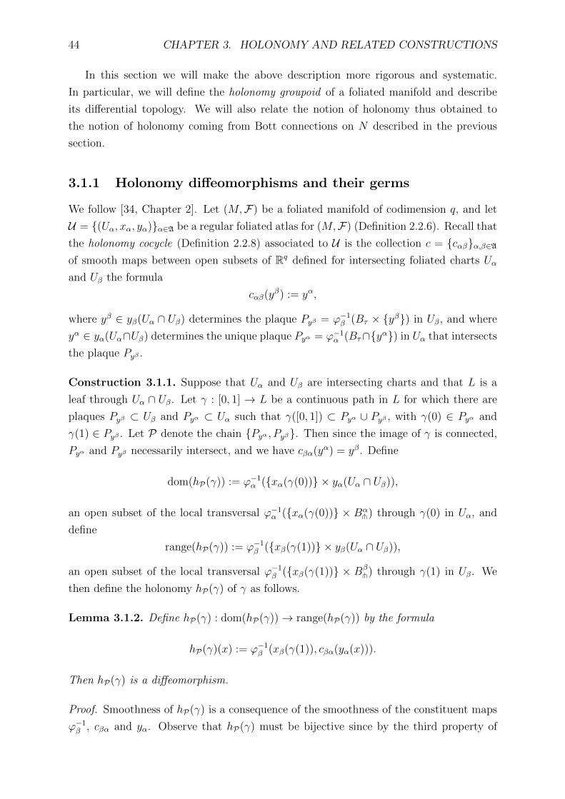
44 CHAPTER 3. HOLONOMY AND RELATED CONSTRUCTIONS
In this section we will make the above description more rigorous and systematic.
In particular, we will define the holonomy groupoid of a foliated manifold and describe
its differential topology. We will also relate the notion of holonomy thus obtained to
the notion of holonomy coming from Bott connections on N described in the previous
section.
3.1.1 Holonomy diffeomorphisms and their germs
We follow [34, Chapter 2]. Let (M,F) be a foliated manifold of codimension q, and let
U = (Uα, xα, yα)α∈A be a regular foliated atlas for (M,F) (Definition 2.2.6). Recall that
the holonomy cocycle (Definition 2.2.8) associated to U is the collection c = cαβα,β∈Aof smooth maps between open subsets of Rq defined for intersecting foliated charts Uα
and Uβ the formula
cαβ(yβ) := yα,
where yβ ∈ yβ(Uα ∩ Uβ) determines the plaque Pyβ = ϕ−1β (Bτ × yβ) in Uβ, and where
yα ∈ yα(Uα∩Uβ) determines the unique plaque Pyα = ϕ−1α (Bτ∩yα) in Uα that intersects
the plaque Pyβ .
Construction 3.1.1. Suppose that Uα and Uβ are intersecting charts and that L is a
leaf through Uα ∩ Uβ. Let γ : [0, 1] → L be a continuous path in L for which there are
plaques Pyβ ⊂ Uβ and Pyα ⊂ Uα such that γ([0, 1]) ⊂ Pyα ∪ Pyβ , with γ(0) ∈ Pyα and
γ(1) ∈ Pyβ . Let P denote the chain Pyα , Pyβ. Then since the image of γ is connected,
Pyα and Pyβ necessarily intersect, and we have cβα(yα) = yβ. Define
dom(hP(γ)) := ϕ−1α (xα(γ(0)) × yα(Uα ∩ Uβ)),
an open subset of the local transversal ϕ−1α (xα(γ(0)) × Bα
t) through γ(0) in Uα, and
define
range(hP(γ)) := ϕ−1β (xβ(γ(1)) × yβ(Uα ∩ Uβ)),
an open subset of the local transversal ϕ−1β (xβ(γ(1)) × Bβ
t) through γ(1) in Uβ. We
then define the holonomy hP(γ) of γ as follows.
Lemma 3.1.2. Define hP(γ) : dom(hP(γ))→ range(hP(γ)) by the formula
hP(γ)(x) := ϕ−1β (xβ(γ(1)), cβα(yα(x))).
Then hP(γ) is a diffeomorphism.
Proof. Smoothness of hP(γ) is a consequence of the smoothness of the constituent maps
ϕ−1β , cβα and yα. Observe that hP(γ) must be bijective since by the third property of

3.1. HOLONOMY 45
Definition 2.2.6, each plaque in Uβ through Uα ∩Uβ meets exactly one plaque in Uα. We
can define the inverse hP(γ)−1 : range(hP(γ))→ dom(hP(γ)) by the formula
hP(γ)−1(y) := ϕ−1α (xα(γ(0)), cαβ(yβ(y)))
and observe that for any x ∈ dom(hP(γ)) we have
hP(γ)−1 hP(γ)(x) =hP(γ)−1(ϕ−1β (xβ(γ(1)), cβα(yα(x)))
)=ϕ−1
α
(xα(γ(0)), cαβ[yβ(ϕ−1
β (xβ(γ(1)), cβα(yα(x))))])
=ϕ−1α
(xα(γ(0)), cαβ(cβα(yα(x)))
)=ϕ−1
α (xα(γ(0)), yα(x))
=x,
where we have used the cocycle property cαβ cβα = id on the fourth line. A symmetric
calculation gives hP(γ) hP(γ)−1 = id on range(hP(γ)), so hP(γ)−1 is indeed the inverse
of hP(γ). The map hP(γ)−1 is smooth for the same reasons that hP(γ) is, whence hP(γ)
is a diffeomorphism.
The map hP(γ) defined on a local transversal through γ(0) is called the holonomy
diffeomorphism of the path γ associated to the plaque chain P . The holonomy of a
longer path, which need not be contained in two intersecting plaques, is defined in a
similar fashion.
Construction 3.1.3. Suppose γ : [0, 1] → L is a continuous path contained in a leaf
L, and that there is a chain P := P0, . . . , Pk of plaques covering the image of γ, with
γ(0) ∈ P0 and γ(1) ∈ Pk, such that Pi ∩ Pi+1 6= ∅ for each i < k. Take a partition
0 = t0 < t1 < · · · < tk = 1 of the interval [0, 1] such that γ(ti) is contained in the plaque
Pi for all i. Define γi+1,i := γ|[ti,ti+1] and P i+1,i := Pi, Pi+1 for each i < k. Thus for
each i < k we obtain the holonomy diffeomorphism hPi+1,i(γi+1,i) : dom(hPi+1,i
(γi+1,i))→range(hPi+1,i
(γi+1,i)) associated to γi+1,i as in Lemma 3.1.2.
The most natural definition of hP(γ) now would be as the successive composition of
each of the hPi+1,i(γi+1,i), but we cannot expect the range of hPi+1,i
(γi+1,i) to be equal to
the domain of hPi+2,i+1(γi+2,i+1) in general. Thus we set P1 := P0, P1,
hP1(γ1) := hP1,0(γ1,0),
and for 1 ≤ i < k we inductively define P i+1 := P1, P2, . . . , Pi+1 and
dom(hPi+1(γi+1)) := hPi(γi)
−1(
range(hPi(γi)) ∩ dom(hPi+1,i(γi+1,i))
),
range(hPi+1(γi+1)) := hPi+1,i
(γi+1,i)(
range(hPi(γi)) ∩ dom(hPi+1,i(γi+1,i))
).

46 CHAPTER 3. HOLONOMY AND RELATED CONSTRUCTIONS
Observe that for each i, dom(hPi(γi)) and range(hPi(γi)) are defined using only fi-
nite intersections of open transverse neighbourhoods, and so are themselves open trans-
verse neighbourhoods of γ(0) and γ(ti) respectively. Setting hPi(γi) :=(hPi,i−1
(γi,i−1) hPi−1
(γi−1))|dom(hPi (γi))
we then have that hPi(γi) : dom(hPi(γi)) → range(hPi(γi)) is a
diffeomorphism. Setting hP(γ) := hPk(γk) we have now the following definition.
Definition 3.1.4. The diffeomorphism hP(γ) : dom(hP(γ)) → range(hP(γ)) of an open
transverse neighbourhood of γ(0) onto an open transverse neighbourhood of γ(1) is called
the holonomy diffeomorphism associated to the path γ and the plaque chain P.
Let us remark that given a regular foliated atlas, the domain of definition of a holon-
omy diffeomorphism depends on the choice of plaque chain used in its definition. In
particular, if given two plaque chains with different initial plaques that nonetheless cover
the same path, there is no reason to think that the domains of the corresponding holon-
omy diffeomorphisms intersect in anything other than the start point of the path they
cover. The next result shows with some straightforward tedium that this ambiguity can
be removed.
Proposition 3.1.5. Let γ : [0, 1]→M be a continuous path contained in a leaf L of M ,
and let P1 and P2 be two distinct plaque chains associated to the regular foliated atlas
that cover the image of γ. Then it can be assumed without loss of generality that P1 and
P2 have the same initial and terminal plaques, and W := dom(hP1(γ))∩ dom(hP2(γ)) is
a nonempty transverse open neighbourhood of γ(0) with hP1(γ)|W = hP2(γ)|W .
Proof. Write P11 = P 1
1 , . . . , P1k and write P2 = P 2
1 , . . . , P2l . That we can assume P1
and P2 to have the same initial and terminal plaques can be seen by concatenating P 11
and P 1k onto the start and end of P2 respectively; because both P1 and P2 cover γ, the
resulting sequence of plaques is again a plaque chain. Choosing corresponding partitions
0 = t11 < · · · < t1k = 1 and 0 < t21 < · · · < t2l = 1 of [0, 1] as in Construction 3.1.3,
and assuming without loss of generality that they have no points in common, we can
amalgamate these partitions into a single partition of [0, 1]. This amalgamated partition
will consist of strings of the form
t1i < t2j < · · · < t2m < t1i+1
and, symmetrically,
t2i < t1j < · · · < t1m < t2i+1.
Since by Construction 3.1.3 the holonomy diffeomorphism associated to a plaque chain
is constructed by successively composing the holonomy diffeomorphisms associated to
pairs of plaques, it suffices to consider the case where P1 = Pα, Pβ consists of only
two plaques, coming from foliated charts (Uα, ϕα = (xα, yα)) and (Uβ, ϕβ = (xβ, yβ))

3.1. HOLONOMY 47
respectively, and P2 = Pα, P1, . . . , Pl, Pβ, with the Pi coming from foliated charts
(Ui, ϕi = (xi, yi)). For simplicity, we will assume that l = 1, and write P2 = Pα, Pδ, Pβ- the general case is similar.
As in Construction 3.1.1, we have dom(hP1(γ)) = ϕ−1α (xα(γ(0))× yα(Uα∩Uβ)) and
hP1(γ)(x) = ϕ−1β (xβ(γ(1)), cβα(yα(x))).
for all x ∈ dom(hP1(γ)). On the other hand, by Construction 3.1.3 we can split P2 into
P21 = Pα, Pδ and P2
2 = Pδ, Pβ, with a corresponding splitting of γ into γ1 : [0, t1]→M
and γ2 : [t1, 1]→M , and regard hP2(γ) as the composition
(hP2
2(γ2) hP2
1(γ1)
)|dom(hP2 (γ)),
where
dom(hP2(γ)) = hP21(γ1)−1
(range(hP2
1(γ1)) ∩ dom(hP2
2(γ2))
).
We have
range(hP21(γ1)) = ϕ−1
δ (xδ(γ(t1)) × yδ(Uα ∩ Uδ))
and
dom(hP22(γ2)) = ϕ−1
δ (xδ(γ(t1)) × yδ(Uδ ∩ Uβ)),
so that
dom(hP2(γ)) =ϕ−1α
(xα(γ(0)) × cαδ(yδ(Uα ∩ Uδ) ∩ yδ(Uδ ∩ Uβ))
)=ϕ−1
α
(xα(γ(0)) × yα
((projBδt ϕδ)
−1(yδ(Uα ∩ Uδ) ∩ yδ(Uδ ∩ Uβ))))
=ϕ−1α
(xα(γ(0)) × yα(Uα ∩ Uδ ∩ Uβ)
)is a transverse open neighbourhood of γ(0) with open, nonempty intersection W =
dom(hP2(γ)) with the transverse open neighbourhood dom(hP1(γ)) of γ(0). Now for
x ∈ W we calculate
hP2(γ)(x) = ϕ−1β (xβ(γ(1)), cβδ cδα(yα(x))) = (xβ(γ(1)), cβα(yα(x))) = hP1(γ)(x)
using the cocycle identity cβδ cδα = cβα on yα(Uα ∩ Uδ ∩ Uβ).
Proposition 3.1.5 tells us that any two choices of plaque chain covering a path in a
leaf determine the same holonomy diffeomorphism on some sufficiently small transverse
open subset. This behaviour is captured in the notion of a germ.
Definition 3.1.6. Let X and Y be topological spaces, let x ∈ X, and let FX,Yx,y be the
collection of continuous functions f : dom(f) → codom(f) where dom(f) is an open
neighbourhood of x and codom(f) is an open neighbourhood of y = f(x). Two elements
48 CHAPTER 3. HOLONOMY AND RELATED CONSTRUCTIONS
f, g ∈ FX,Yx,y are said to have the same germ at x if there is an open neighbourhood U of
x such that U ⊂ dom(f) ∩ dom(g) and f |U = g|U .
Lemma 3.1.7. Let X, Y and Z be topological spaces, and let x ∈ X.
1. for y ∈ Y , the relation ∼ on FX,Yx,y defined by f ∼ g if and only if f and g have the
same germ is an equivalence relation, and we denote the equivalence class of f by
fx or germx(f),
2. if f ∈ FX,Yx,y and g ∈ F Y,Z
y,z then g f |f−1(dom(g)) ∈ FX,Zx,z and the formula gyfx :=
(g f |f−1(dom(g)))x is a well-defined composition,
3. if f ∈ FX,Yx,y is a local homeomorphism then f−1 ∈ F Y,X
y,x with fxf−1y = idy and
f−1y fx = idx.
Proof. That having the same germ is an equivalence relation is straightforward, with the
exception of transitivity. For this, suppose that there is an open neighbourhood U of x
with U ⊂ dom(f) ∩ dom(g) and f |U = g|U , and that there is an open neighbourhood V
of x with V ⊂ dom(g)∩ dom(h) and g|V = h|V . Then V ∩U is an open neighbhourhood
of x contained in dom(f) ∩ dom(h) and f |U∩V = g|U∩V = h|U∩V .
The second assertion is true because f−1(dom(g)) is a nonempty open subset of
dom(f), and if f ∈ fx and g ∈ gx are any other two functions agreeing with f and
g on open sets U and V respectively, then the composition g f |f−1(dom(g)) agrees with
gf |f−1(dom(g)) on the open set f−1(V )∩U . Finally the third assertion follows easily from
the second.
The composition and inversion structure on germs will be important for the algebraic
structure of the holonomy groupoid.
Let us now come back to our foliated manifold (M,F), of codimension q, with regular
foliated atlas U = (Uα, xα, yα)α∈A, and refine our definition of holonomy. Let γ : [0, 1]→L be a continuous path in a leaf L of F , with γ(0) = x and γ(1) = y. Recall that given
a plaque chain P covering γ, hP(γ) : dom(hP(γ)) → range(hP(γ))) is a diffeomorphism
of transverse open neighbourhoods about x and y respectively. We consider the germ
germx(hP(γ)) of this diffeomorphism.
Definition 3.1.8. Let P be any plaque chain covering γ. The germinal holonomy γx
of the path γ is defined to be
γx := germx(hP(γ))
By Proposition 3.1.5, the definition given above is independent of the plaque chain
chosen. The germinal holonomy of a path is also robust up to homotopic perturbations.
Lemma 3.1.9. Let γ be any path in L that is fixed-endpoint-homotopic to γ in L. Then
γx = γx.
3.1. HOLONOMY 49
Proof. Suppose that γt is a fixed-endpoint-homotopy with γ1 = γ and γ0 = γ, t ∈ [0, 1].
Then (γt)x is locally constant in t because for sufficiently small changes in t one need not
change the plaque chain used to define (γt)x. Since [0, 1] is connected, (γt)x is globally
constant.
That the germ of the holonomy of a path is the same for all paths in its homotopy
class allows us to make the following important observation.
Corollary 3.1.10. If γ : [0, 1] → M is a path in a leaf L of F , with γ(0) = x and
γ(1) = y, then there is a smooth path γ : [0, 1] → M with the same endpoints as γ such
that γx = γx.
Proof. By [30, Proposition 17.8], we can always find a smoothly immersed path γ that is
endpoints-homotopic to γ. By Lemma 3.1.9, γ has the same germ at x as γ.
Using Corollary 3.1.10 we can assume without loss of generality that all paths we
consider are smooth. Thus the terminology “path” will be used to mean “smooth path”.
We can now use the composition structure observed for germs in Lemma 3.1.7 to give
the collection of all germinal holonomies an algebraic structure.
Construction 3.1.11. For x, y ∈M contained in a leaf L, we define
Gyx := γx : γ is a path in L from x to y.
Then for x, y, z ∈ L we have a well-defined map m : Gzy×Gyx → Gzx defined by the
composition of germs
m(δy, γx) := δy γx = (δγ)x
for all δy ∈ Gzy and γx ∈ Gyx, where δγ denotes the concatenation of the paths δ and γ.
Due to the fact that our germs arise from diffeomorphisms, we also have an inversion
map ι : Gyx → Gxy defined by
ι(γ)y := γ−1y = (γ−1)y,
where γ−1 is the path γ with the opposite orientation. It is then clear that we have
m(γx, (γ−1)y) = idy and m((γ−1)y, γx) = idx. We also have the obvious maps r, s : Gyx →
M defined by r(Gyx) := y and s(Gyx) = x.
For x ∈ M let Lx be the leaf through x and define G :=⊔x∈M,y∈Lx G
xy . Then G is
a groupoid (see Definition B.1.1) with unit space G(0) = M . The range and source are
defined by the equations
r(Gyx) := y s(Gyx) := x
for all x, y contained in the same leaf. The multiplication Gx×Gx → G and inversion
Gx → Gx are given for all x ∈ M by maps m and ι. Associativity of the multiplication

50 CHAPTER 3. HOLONOMY AND RELATED CONSTRUCTIONS
is due to the associativity of function composition which implies associativity of the
composition of germs. Similarly, (δγ)−1z = γ−1
y δ−1z is true for all (δ, γ) ∈ Gzy×Gyx because
if f and g are composable homeomorphisms then (f g)−1 = g−1 f−1.
Definition 3.1.12. The groupoid G obtained from F as in Construction 3.1.11 is called
the holonomy groupoid of (M,F). We will from here on refer to elements of G using
the letters u, v, w.
In order to treat foliations using the tools of noncommutative geometry, the holonomy
groupoid must be equipped with a differential topology under which it becomes a Lie
groupoid. This will be our concern in the next subsection.
3.1.2 Differential topology of the holonomy groupoid
The regular foliated atlas used to define the holonomy of a foliated manifold (M,F) can be
used to give a differential topology to the holonomy groupoid G of F . This construction
is due to Winkelnkemper [153], and a very thorough and thoughtful discussion of the
construction and its relationship with the groupoid built from homotopy classes of paths
in leaves, called the homotopy or monodromy groupoid, can be found in [138]. Equipped
with a differentiable structure in this manner, G will itself be a foliated manifold whose
leaves are the range and source fibres. Unfortunately, the topology of G obtained in this
way will in general be non-Hausdorff.
Construction 3.1.13. Fix a plaque chain P = P1, . . . , Pk coming from the regular
foliated atlas U of (M,F), contained in a leaf L of F . Denote the corresponding initial and
terminal charts by (Us, ϕs) and (Ur, ϕr) respectively, and denote the ranges of ϕr = (xr, zr)
and ϕs = (xs, zs) by Brτ ×Br
t and Bsτ ×Bs
t respectively, where Brτ , B
sτ are open rectangles
in Rp and where Brt, B
st are open rectangles in Rq. Then as in Definition 3.1.4, for each
x ∈ P1 there is an open set V P ⊂ Bst for which UPx := ϕ−1
s (xs(x) × V P) is an open
transverse neighbourhood of x on which hP(γ) is a diffeomorphism onto its image for any
continuous path γ : [0, 1]→M that is covered by P with γ(0) = x.
For any smooth path γ : [0, 1]→M that is covered by P and for any q ∈ [0, 1] we let
γq : [0, 1] → M denote the smooth path t 7→ γ(qt), whose image is contained in that of
γ and with initial point γ(0) and end point γ(q). Letting Pq denote the shortest plaque
sub-chain of P which covers γq we have that hPq(γq) is a diffeomorphism of UPγ(0) onto its
image. We then define Hγ : UPγ(0) × [0, 1]→M by
Hγ(x, t) := hPt(γt)(x),
which is a smooth map by the smoothness of γt. In particular, for each x ∈ UP the map
Hγx : t 7→ Hγ(x, t) is a smooth path in a leaf close to L.
3.1. HOLONOMY 51
Now every (a, b, c) ∈ Brτ×Bs
τ×V P determines an element ψ−1P (a, b, c) in G represented
by any path of the form Hγ
ϕ−1s (b,c)
, where γ is some path in L covered by P with xs(γ(0)) =
b and xr(γ(1)) = a. Since any two such paths γ have the same germinal holonomy,
this assignment gives a well-defined map ψ−1P : Br
τ × Bsτ × V P → G, whose range we
denote by WP . The map ψ−1P is moreover injective because if (a, b, c) 6= (a′, b′, c′) are
two distinct elements in Brτ × Bs
τ × V P then ψ−1P (a, b, c) and ψ−1
P (a′, b′, c′) must have
either different range or source and so must be distinct elements of G. We denote by
ψP : WP → Brτ × Bs
τ × V P the inverse of ψ−1P , and obtain a topology on G by declaring
the WP to be a subbasis.
Lemma 3.1.14. The sets WP , defined for plaque chains P derived from the regular
foliated atlas U of (M,F), constitute a subbasis for a locally compact, second-countable,
locally Hausdorff topology on G. With respect to this topology, the range and source maps
are open and their fibres are covering spaces of the leaves of F , and so are Hausdorff.
Proof. Since the sets WP are all isomorphic as sets to locally compact, Hausdorff, open
rectangles in R2p+q, it suffices to find a countable subcollection of the WP that cover
G; such a subcollection will define a subbasis for the desired locally compact, second-
countable, locally Hausdorff topology. That this can be done is a consequence of two
facts. First is the countability of the regular foliated atlas for (M,F), which ensures only
countably many plaque chains will cover any representative of any element of G. Second
is the fact that for all x, y contained in any leaf L of F , the set Gyx is at most countable
due to it being the range of a surjection from the countable set of homotopy classes of
paths in the manifold L joining x to y.
We now show that the source map is open and has Hausdorff fibres. The proof
for the range map is similar. Since the WP are a subbasis for the topology of G, to
show that s is open we will show that if P1 and P2 are plaque chains, then the set
s(WP1 ∩WP2) is open (the proof for arbitrary finite intersections is similar). For i = 1, 2
let Li denote the leaf containing the plaque chain P i. If WP1 ∩WP2 is empty then we
are done. Suppose instead that u ∈ WP1 ∩WP2 6= ∅. Then the initial (resp. terminal)
plaques of P1 and P2 belong to foliated charts whose intersection must contain s(u)
(resp. r(u)) and is therefore nonempty. Thus by a similar argument to Proposition 3.1.5
we can assume without loss of generality that the initial (resp. terminal) plaque of P1
belongs to the same foliated chart (Us, ϕs = (xs, ys)) (resp. (Ur, ϕr = (xr, yr))) as the
initial (resp. terminal) plaque of P2. Let γi be any path in the leaf Li that is covered
by the plaque chain P i, and for which ys(γi(0)) = ys(s(u)) and yr(γi(1)) = yr(r(u)).
Then, letting L denote the leaf through r(u) and s(u), the groupoid element u can be
represented by either of the paths γi := Hγis(u) : [0, 1] → L, i = 1, 2, defined for the γi
and P i as in Construction 3.1.13. Let P i be any plaque chain in L covering γi, define
P := P1, and V P := ys(
dom(hP1(γ1)) ∩ dom(hP2
(γ2)))⊂ ys(Us). Then in a similar
52 CHAPTER 3. HOLONOMY AND RELATED CONSTRUCTIONS
manner to Construction 3.1.13 we define Wu to be the collection of elements of G that
are represented by any path of the form H γ
ϕ−1s (b,c)
, where γ is any path in L covered by
P and where (b, c) ∈ xs(Us)× V P . Then Wu ⊂ WP1 ∩WP2 is a neighbourhood of u, and
s(Wu) = ϕ−1s (xs(Us)×V P) is open. Since WP1 ∩WP2 can be written as the union of such
sets Wu, we have that s(WP1 ∩WP2) is open, hence s is an open map.
Now fix x ∈ M and let L be the leaf through x. We show that r : Gx → L is a
covering map, hence that Gx is Hausdorff by the Hausdorffness of L. Fix y ∈ L and
a plaque P containing y. For each u contained in the countable set Gyx, there exists a
plaque chain Pu covering a representative of u which without loss of generality has P as
its terminal plaque. Then the open subset Pu := WPu ∩ Gx of Gx consists precisely of all
the classes of paths that begin at x and are covered by Pu. Since the terminal plaque of
each Pu is equal to P , each Pu identifies homeomorphically via the range map with P .
Consequently
r|−1Gx (P ) =
⋃u∈Gyx
Pu.
Moreover the Pu are all mutually disjoint since they correspond to distinct holonomy
classes, so in fact
r|−1Gx (P ) =
⊔u∈Gyx
Pu,
making r : Gx → L a covering map.
A differentiable structure on G can also be defined by declaring the pairs (WP , ψP) to
be charts.
Lemma 3.1.15. The pairs (WP , ψP) are charts for a smooth structure on G. With respect
to this smooth structure, the range, source, and multiplication maps are smooth, hence
continuous, while the inversion map is a diffeomorphism. Moreover, the range and source
fibres are embedded, smooth, Hausdorff submanifolds of G.
Proof. If P is a plaque chain we let ϕr := (xr, zr) and ϕs := (xs, zs) denote the foliated
chart maps corresponding respectively to the terminal and initial charts defining P . Ob-
serve that if u ∈ WP , then ψP(u) = (xr(r(u)), xs(s(u)), zs(s(u))). Thus if (WPi , ψPi),
i = 1, 2, are any two intersecting charts in G, the foliated charts (U ri , ϕ
ri ) and (U s
i , ϕsi ) of
(M,F) corresponding respectively to their initial and terminal plaques have U r1 ∩U r
2 and
U s1 ∩ U s
2 nonempty, with transition functions of the form
ϕr1 (ϕr2)−1(x, z) = (xr12(x, z), zr12(z)), (x, z) ∈ Brτ ×Br
t,
and
ϕs1 (ϕs2)−1(y, z) = (xs12(y, z), zs12(z)), (y, z) ∈ Bsτ ×Bs
t,

3.1. HOLONOMY 53
by Lemma 2.2.2. Therefore the transition function ψP1 ψ−1P2
for the charts WP1 and WP2
on G has the form
ψP1 ψ−1P2
(x, y, z) = (xr12(x, z), xs12(y, z), zs12(z)), (x, y, z) ∈ Brτ ×Bs
τ ×Bst,
which is smooth by the smoothness of the xr12, xs12 and zs12. Hence the charts (WP , ψP)
determine a smooth structure on G.
Smoothness of s is now true because on any chart WP ∼= Brτ × Bs
τ × Bst we have
that s(x, y, z) = (y, z) is smooth, and similarly for the range. On any such chart in-
version has the form (x, y, z) 7→ (y, x, h(z)) for a smooth function h, hence is smooth
also. Moreover, on two such charts, multiplication takes the form of the smooth map
(w, x, h(z)) · (x, y, z) = (w, y, z), hence is smooth as a map G ×s,r G → G equipped with
the canonical differentiable structure.
The final claim is a consequence of the fact that the range and source fibres are covering
spaces of the leaves of F , so must be smooth manifolds. Their topology moreover coincides
by definition with the subspace topology inherited from G, and so they are embedded
submanifolds of G.
That the holonomy groupoid of a foliation is a smooth manifold gives it a great deal
of useful structure. Indeed, we will see in later sections how the smooth structure of the
holonomy groupoid can be used to construct differential forms on the holonomy groupoid
from which we can extract the Godbillon-Vey invariant as a cyclic cocycle. That the
holonomy groupoid is not always Hausdorff, however, will make the coming chapters
somewhat more difficult than they might be otherwise, so we will take some time now to
study the Hausdorffness of the holonomy groupoids of the Reeb foliation of S3 (which has
non-Hausdorff holonomy groupoid) and of suspension foliations (which, under reasonable
assumptions, have Hausdorff holonomy groupoid).
Example 3.1.16 (Reeb foliation of S3). To see that a space is non-Hausdorff it suffices
to construct a sequence in that space which converges to two distinct points. That this
occurs for the holonomy groupoid of the Reeb foliation F of S3 can be seen by constructing
a convergent sequence of loops with trivial holonomy (which must therefore converge in
G to the class of a trivial loop), that also converges to a loop on the closed leaf that has
nontrivial holonomy.
It will be helpful to consider the two separate copies of the Reeb foliation of the solid
torus D2 × S1 that are glued together along their boundary. On the boundary S1 × S1,
one considers a loop γ0 of the form t 7→ (eiθ0 , eit), t ∈ [0, 2π], for any fixed θ0. Thus γ0
wraps around the torus in the poloidal direction as depicted in Figure 3.2.
Regard now the second copy of S1 as the boundary of the disc D2, and consider the
Reeb foliated solid torus S1 × D2. Take a sequence of interior leaves Ln of this solid

54 CHAPTER 3. HOLONOMY AND RELATED CONSTRUCTIONS
Figure 3.2: The path γ0 on the closed leaf
torus, each of which is diffeomorphic to R2. In each Ln take a loop γn that goes around
the origin, in such a way that when embedded into S1×D2 the loops γn converge to the
poloidal loop γ0 on the boundary. Such loops are depicted in Figure 3.3a. Then every γn
is contractible to a point in the leaf Ln, and so has trivial holonomy. Consequently, the
sequence in G determined by the γn converges to the class of the constant loop t 7→ (eiθ0 , 1)
on the closed leaf.
On the other hand, by construction the γn also approach the loop γ0 on the closed
leaf, which does not have trivial holonomy. To see this one must consider the second copy
of the Reeb foliated solid torus D2× S1. From the perspective of this second solid torus,
γ0 is a toroidal loop. Thus if T is some transversal in D2 × S1 through the basepoint of
γ0, then the holonomy map on T defined by γ0 is defined by transport along a toroidal
path as in Figure 3.3b. This transport map is clearly not the identity, so γ0 cannot have
trivial holonomy in S3.
(a) A poloidal loop with trivial holon-omy.
(b) A toroidal path with nontrivialholonomy.
Figure 3.3: Paths that are close to γ0.

3.2. EQUIVARIANT BUNDLES 55
Example 3.1.17 (Suspension foliations). Let M be any connected manifold and M
its universal cover, with covering map p : M → M and deck transformation group
π1(M) = Γ. If T is any other connected manifold, with diffeomorphism group Diff(T ),
and h : Γ→ Diff(T ) is a homomorphism, then Γ acts on M×T by the formula (m, t)·γ :=
(m · γ, h(γ−1)t). This action preserves the leaves M × t, t ∈ T , of the trivial foliation
of M × T , so gives a foliation F of (M × T )/Γ. Foliations constructed in this way are
called suspension foliations [35, Section 3.1].
If the action of Γ on T is locally free, in the sense that h(γ)t = t for all t in some
open subset U of T only if γ = id, then the holonomy groupoid of ((M × T )/Γ,F) is
diffeomorphic to the Hausdorff groupoid (M×M×T )/Γ [126, Section 2]. Here we denote
the class of (m,n, t) by [m,n, t]. The range and source are then defined by
r([m,n, t]) := [m, t], s([m,n, t]) = [n, t],
while [m,n, t] and [m′, n′, t′] are composable if and only if there is γ ∈ Γ such that
n = m′ · γ and t = h(γ−1)t′. For such composable pairs, the product is given by the
formula
[m,n, t] · [m′, n′, t′] = [m · γ−1, n′, t′].
3.2 Equivariant bundles
For the entirety of this section let (M,F) be a transversely orientable foliated manifold
of codimension q, with normal bundle πN : N → M and holonomy groupoid G. Since Ghas M as its unit space, M is clearly a G-space (see Definition B.1.3), but there are other
natural G-spaces associated to (M,F) that will be important in the later chapters. The
first example of such a G-space is the normal bundle itself.
Proposition 3.2.1. The normal bundle N is a G-space.
Proof. The bundle N can be trivialized over any foliated chart (U, (x, y)) of (M,F), with
U ∼= Bτ ×Bt for open rectangles Bτ ⊂ Rp and Bt ⊂ Rq, via the canonical identifications
N |U = (TM |U)/(T F |U) ∼= T (Bτ ×Bt)/(TBτ ×Bt) ∼= Bτ × (TBt) ∼= U × Rq .
Under this identification, N |U consists of vectors that are tangent to the local transversals
in the chart U .
In particular, for u ∈ G, any representative path γ contained in a leaf L of F , and any
associated plaque chain P covering the image of γ coming from charts in U , the derivative
of the associated holonomy diffeomorphism hP(γ) : dom(hP(γ)) → range(hP(γ)) there-
fore defines a linear map (dhP(γ))s(u) : Ns(u) → Nr(u). Since the derivatives of any two
diffeomorphisms with the same germ at a particular point are identical at that point, the
56 CHAPTER 3. HOLONOMY AND RELATED CONSTRUCTIONS
linear map (dhP(γ))s(u) is independent of the choices of γ and P , and therefore gives a
well-defined linear isomorphism u∗ : Ns(u) → Nr(u) for which
u∗ v∗ = (uv)∗
for all (u, v) ∈ G(2). Since the action of G on M is smooth, the map G ×s,πNN → N
defined by (u, n) 7→ u∗n thus obtained is also smooth, and therefore defines a G-bundle
structure on N .
The action of the holonomy groupoid G of a foliated manifold (M,F) on its nor-
mal bundle N is referred to as the holonomy transport on N . We wish to justify this
nomenclature by showing that this action of the holonomy groupoid on N agrees with the
parallel transport defined by any Bott connection on N . Before we can do this, we need
to show how the total space of N , and of fibre bundles associated to it, can be endowed
with a canonical foliation. The result we give is essentially known (see for instance [119,
Section 4]), but it is difficult to find a proof in the literature. We give a proof here.
Proposition 3.2.2. Let (M,F) be a foliated manifold of codimension q. Let π : B →M
be a smooth, locally trivial fibre bundle over M , with typical fibre a connected m-manifold
Y . Suppose furthermore that B carries an action G ×s,πB → B of G. Then the total
space B carries a foliation FB of codimension q +m such that
1. the fibres of B over M are all transverse to the leaves of FB, and
2. the leaves of FB are mapped by π to the leaves of F , and dπ : TB → TM restricts
to a fibrewise-isomorphism of T FB onto T F .
3. the holonomy groupoid GB of (B,FB) is isomorphic to the crossed product GnB.
Proof. We will show that the orbits of G in B, defined to be the equivalence classes of
the equivalence relation
b1 ∼ b2 ⇔ there is u ∈ Gπ(b1)π(b2) such that b1 = u · b2,
define the leaves of a foliation of B of the stated type.
First we must show that the orbits of G are immersed submanifolds of B. For this,
let GnB be the groupoid obtained from the action of G on B as in Definition B.1.3,
and let rB, sB be its range and source maps. Every orbit of G in B then identifies with
rB((GnB)b) for some b ∈ B. Since r|Gπ(b)is a local diffeomorphism onto its image so too
is rB|(G nB)b , and therefore rB((GnB)b) is an immersed submanifold of B.
Now let U = (Uα, ϕα)α∈A be a foliated atlas for M , and assume without loss of
generality that over each Uα one has B|Uα ∼= Uα × Y . Then for any coordinate chart
V ∼= Rm of Y we obtain for each α a foliated chart Uα × V ∼= Bατ × Bα
t × Rm of B. For

3.2. EQUIVARIANT BUNDLES 57
any b = (x, y) ∈ Uα × V we consider the orbit rB((GnB)b) through b. Let Tαx denote
the local transversal through x in Uα. Then each u ∈ GTαxx is associated to some plaque
Pαu in Uα containing r(u). We let S ⊂ GTαxx denote the set of those u ∈ GTαxx for which
u · y := projV (u · b) ∈ V . Then r−1B ((GnB)b) ∩ (Uα × V ) =
⋃u∈S P
αu × u · y is a union
of plaques. Therefore the collection of all Uα × V , where V is any chart in Y , defines a
foliated atlas for B and makes (B,FB) a foliated manifold of codimension q +m.
That the fibres of B are transverse to the leaves of FB and that the leaves of FB are
mapped by π to those of F can be seen by the structure of the foliated charts for B. The
coincidence of GB with GnB is a consequence of the fact that the leaves of FB are by
construction the orbits of G in B.
Definition 3.2.3. We say that a bundle π : B →M over a foliated manifold (M,F) is a
G-equivariant bundle or simply a G-bundle if it satisfies the hypotheses of Proposition
3.2.2. If B = E is a vector bundle over M and G acts by linear isomorphisms of the
fibres, we refer to π : E →M as a G-equivariant vector bundle or simply a G-vector
bundle. If a G-vector bundle E is equipped with a Euclidean (resp. Hermitian) structure
for which the action of G is by orthogonal (resp. unitary) isomorphisms, then we say that
E is a G-equivariant Euclidean (resp. Hermitian) bundle.
Remark 3.2.4. Note that by Proposition 3.2.2, any G-bundle is a foliated bundle in the
sense of [102, p. 20]. When π : B →M is a G-bundle we use the following notation.
1. The action G ×s,πB → B is denoted by
(u, b) 7→ uB · b,
for all u ∈ G and b ∈ Bs(u).
2. The normal bundle of (B,FB) is denoted by πNB : NB → B. The corresponding
action of GB on NB can, in light of the final item in Proposition 3.2.2, be regarded
as a map G ×s,ππNBNB → NB and will be denoted
(u, n) 7→ uB∗ n
for all u ∈ G and n ∈ (NB)b with b ∈ Bs(u).
3. That uB· : Bs(u) → Br(u) is a diffeomorphism for each u ∈ G implies that the vertical
tangent bundle V B := ker(dπ) is a foliated vector bundle over the foliated manifold
(B,FB). We denote the action of G on V B by
(u,X) 7→ uV B∗ X
for all u ∈ G and X ∈ (V B)b with b ∈ Bs(u).
58 CHAPTER 3. HOLONOMY AND RELATED CONSTRUCTIONS
Propositions 3.2.1 and 3.2.2 tell us that the normal bundle N of any foliated manifold
is a foliated vector bundle. Using this fact, we can prove that the action of the holonomy
groupoid G onN agrees with the parallel transport onN arising from any Bott connection.
This result appears to be folklore, and it is difficult to find a proof in the literature. We
give our own proof here, based on Proposition 3.2.2.
Proposition 3.2.5. Let (M,F) be a foliated manifold, G its holonomy groupoid and N
its normal bundle. Let ∇[ be any Bott connection on N . Then for any u ∈ G, the map
u∗ : Ns(u) → Nr(u) agrees with the parallel transport map P∇[
γ : Ns(u) → Nr(u) defined for
any smooth path γ representing u.
Proof. Fix u ∈ G and let γ : [0, 1] → M be any smooth path representing u. For each
n ∈ Ns(u), the parallel transport of n along γ is by definition σn(γ(1)) ∈ Nr(u), where σn
is the unique section of N over γ for which σn(γ(0)) = n and for which ∇[γσn = 0 along
γ. The path σn γ is precisely the unique path in the leaf of the foliation FN through n
whose image under the projection onto M is γ.
Now for each t ∈ [0, 1] we let γt be the path γt(t′) := γ(tt′) which starts at γ(0) and
ends at γ(t), and observe that the family γtt∈[0,1] uniquely determines a path ut in Gs(u)
from s(u) to u with the property that r(ut) = γ(t). Then the path σn γ in the leaf of
FN through n coincides by Proposition 3.2.2 with the path t 7→ ut∗n. Thus in particular
P∇[
γ (n) = σn(γ(1)) = u1∗n = u∗n
as claimed.
A particularly important class of G-bundles are G-principal bundles - that is, principal
bundles carrying an action of G that commutes with the right action of the associated
structure group. We will see many important examples of these bundles in the remainder
of the thesis. For now, let us give a useful general result concerning G-principal bundles.
Proposition 3.2.6. Let G be a connected Lie group with Lie algbera g, and let π : P →M be a principal G-bundle which moreover carries an action G ×s,πP → P of G that
commutes with the right action of G. Then the fundamental vector fields
V Xp :=
d
dt
∣∣∣∣t=0
(p · exp(tX))
defined for X ∈ g are invariant under the action of G. Thus in the associated trivialisation
P × g 3 (p,X) 7→ V Xp ∈ V P of V P we have
uV P∗ (p,X) = (uP · p,X)
for all u ∈ G, p ∈ P and X ∈ g.
3.2. EQUIVARIANT BUNDLES 59
Proof. We calculate
uV P∗ V Xp =
d
dt
∣∣∣∣t=0
(uP · (p · exp(tX))) =d
dt
∣∣∣∣t=0
((uP · p) · exp(tX)) = V XuP ·p
for all X ∈ g, u ∈ G and p ∈ Ps(u).
3.2.1 The frame bundle
For the entirety of this subsection, we continue to assume that (M,F) is a transversely
orientable, foliated manifold of codimension q, with holonomy groupoid G. Canonically
associated to any such manifold is the positively oriented transverse frame bundle.
Definition 3.2.7. The positively oriented transverse frame bundle πFr+(N) : Fr+(N) →M , is the principal GL+(q,R)-bundle whose fibre Fr+(N)x over x ∈ M consists of all
positively oriented linear isomorphisms φ : Rq → Nx. The space Fr+(N) comes equipped
with a G-action G ×s,πFr+(N)Fr+(N)→ Fr+(N) defined by
(u, φ) 7→ u∗ φ : Rq → Nr(u)
for all u ∈ G and φ ∈ Fr+(N)s(u). Consequently Fr+(N) is also a G-bundle over M , with
foliation that we will denote by F1 and holonomy groupoid G1 := GnFr+(N).
Now the principal bundle πFr+(N) : Fr+(N) → M is the principal frame bundle for
the oriented vector bundle N . Thus if ∇ is any connection on N , there is a connection
1-form α ∈ Ω1(Fr+(N); gl(q,R)) (see Definition D.2.8, Example D.2.9) on Fr+(N) such
that if χ : U → Fr+(N) is a local frame field over U ⊂M , then α pulls back via χ to the
local connection form of ∇ expressed in the frame χ.
The next three results give a detailed description of the connection 1-form α[ ∈Ω1(Fr+(N); gl(q,R)) associated to any Bott connection ∇[ on N and its relationship to
the foliation FFr+(N) of Fr+(N) arising from Proposition 3.2.2. These results will be
needed for our groupoid characteristic map in the next chapter. The first of these results
is well-known [22, Section 2], while the two that follow do not appear explicitly in the
literature.
Lemma 3.2.8. Let ∇[ be a Bott connection on N , and let U be a foliated chart for
(M,F) in which ∇[ has corresponding connection form α ∈ Ω1(U ; glq(R)). Then for any
X ∈ Γ∞(U ;T F), α(X) = 0 identically on U .
Proof. Let (x1, . . . , xp, z1, . . . , zq) be foliated coordinates for U , and for σ ∈ Γ∞(U ;N)
write
σ =
q∑i=1
σi∂
∂zi

60 CHAPTER 3. HOLONOMY AND RELATED CONSTRUCTIONS
and
X =
p∑j=1
X i ∂
∂xj,
where the σi and Xj are real-valued smooth functions on U . By definition
∇[Xσ = projspan ∂
∂zj[X, σ] =
q∑i=1
p∑j=1
Xj ∂σi
∂xj∂
∂zi=
q∑i=1
dσi(X)∂
∂zi,
which, together with the equation ∇[ = d+α as in Lemma C.0.2, necessitates α(X) = 0
as claimed.
Proposition 3.2.9. Let ∇[ be a Bott connection on N , with associated connection 1-form
α[ ∈ Ω1(Fr+(N); gl(q,R)). Then T FFr+(N) ⊂ ker(α[).
Proof. It suffices to work locally. Given any foliated chart U of (M,F) with associated
local frame χU : Rq → N |U , we have a trivialisation Fr+(N)|U ∼= U ×GL+(q,R) given by
φ 7→ (πFr+(N)(φ), gφ),
where gφ is the unique element of GL+(q,R) such that φ · gφ = χU . Let αU be the local
connection form of ∇[ in the foliated chart U , and let ωMC be the Maurer-Cartan form
on GL+(q,R) defined by
ωMCg (X) := dLg−1(X) ∈ gl(q,R),
where L denotes left multiplication. Then letting π1 : U × GL+(q,R) → U and π2 :
U ×GL+(q,R)→ GL+(q,R) be the projections, as in Lemma C.0.8 α[ can be expressed
in this trivialisation by
α[(x,g) := Adg−1
(π∗1αU
)(x,g)
+(π∗2ω
MC)
(x,g).
Now since vectors in T FFr+(N) correspond in this trivialisation to vectors in T F by the
differential of the projection π1, Lemma 3.2.8 tells us that T FFr+(N) lies in the kernel of
α[.
The choice of a Bott connection form α[ ∈ Ω1(Fr+(N); gl(q,R)) can now be seen to
determine a trivialisation of the normal bundle NFr+(N) of FFr+(N) and an associated Bott
connection ∇Fr+(N) on NFr+(N).
Proposition 3.2.10. Let α[ ∈ Ω1(Fr+(N); gl(q,R)) be the connection form of a Bott
connection for N . Then the differential dπFr+(N) : T Fr+(N) → TM of the projection
descends for each φ ∈ Fr+(N) to a linear isomorphism πφ : (ker(α[)/T FFr+(N))φ →
3.2. EQUIVARIANT BUNDLES 61
NπFr+(N)(φ). We therefore obtain a trivialisation
Fr+(N)× Rq 3 (φ, v) 7→ (π−1φ φ)(v) ∈ (ker(α[)/T FFr+(N)).
Let 1q2 denote the identity map on the vector space gl(q,R) = Rq2
. Then with respect to
the corresponding trivialisation NFr+(N) = V Fr+(N) ⊕ (ker(α)/T FFr+(N))∼= Fr+(N) ×
(gl(q,R)⊕Rq), the equation ∇Fr+(N) := d+(1q2⊕α[) defines a Bott connection on NFr+(N).
Proof. The first claim is true by dimension count. Now let us regard the trivialisation
NFr+(N)∼= Fr+(N) × (gl(q,R) ⊕ Rq). For any X ∈ Γ∞(Fr+(N);T FFr+(N)) and for any
section σ ∈ C∞(Fr+(N); gl(q,R)⊕ Rq) of NFr+(N) we have
∇Fr+(N)X (σ) = dσ(X) + (1q2 ⊕ α[(X))(σ) = dσ(X) = [X, σ],
so ∇Fr+(N) := d+1q2⊕α[ is indeed a Bott connection for the normal bundle of the foliated
manifold (Fr+(N),FFr+(N)) by Definition 2.4.15.
Let us end this subsection with a characteristic map for Fr+(N). For this, it will be
necessary to make some observations of the structure of the differential graded algebra
of differential forms on Fr+(N).
Construction 3.2.11. Because Fr+(N) carries a right action R of GL+(q,R), the dif-
ferential forms Ω∗(Fr+(N)) on Fr+(N) also carry an action of GL+(q,R) defined by pull-
backs:
g · ω := R∗g−1ω, g ∈ GL+(q,R), ω ∈ Ω∗(Fr+(N)).
Note that this action preserves the grading of Ω∗(Fr+(N)). Moreover contraction with the
fundamental vector field V X on Fr+(N) associated to any X ∈ gl(q,R) (see Proposition
3.2.6) defines a derivation iX of degree -1 on Ω∗(Fr+(N)). For X ∈ gl(q,R), we let
LXω :=d
dt
∣∣∣∣t=0
(exp(tX) · ω), ω ∈ Ω∗(Fr+(N))
denote the infinitesimal GL+(q,R)-action induced by the action of GL+(q,R) on the
algebra Ω∗(Fr+(N)). Then the triple (Ω∗(Fr+(N)), d, i) has the following properties:
iXiY = −iY iX , giXg−1, iXd+diX = LX , X, Y ∈ gl(q,R), g ∈ GL+(q,R).
This information can all be summarised by referring to the triple (Ω∗(Fr+(N)), d, i) as
a GL+(q,R)-differential graded algebra. We have included a detailed exposition on G-
differential graded algebras, their cohomology and their applications to characteristic
classes in Appendix D.2 for the reader’s convenience.

62 CHAPTER 3. HOLONOMY AND RELATED CONSTRUCTIONS
Of particular importance to us are those elements of Ω∗(Fr+(N)) that are invariant
under the action of GL+(q,R), and which are annihilated by the contractions iX de-
fined for X ∈ so(q,R). Such elements are referred to as SO(q,R)-basic elements. We
refer to Definition D.2.2 for the general notion of basic elements occuring in the con-
text of G-differential graded algebras. We prove in particular in Example D.2.6 that
the SO(q,R)-basic elements of Ω∗(Fr+(N)) identify naturally with the differential forms
Ω∗(Fr+(N)/ SO(q,R)) on the quotient of Fr+(N) by the right action of SO(q,R). This
algebra of SO(q,R)-basic elements is the receptacle of the characteristic map that we give
below.
Theorem 3.2.12. For any Bott connection form α[ on Fr+(N) we obtain a homomor-
phism φα[ : WOq → Ω∗(Fr+(N)/ SO(q,R)), whose induced map on cohomology does not
depend on the Bott connection chosen.
Proof. By Theorem D.2.11, we obtain a homomorphism φα[ : W (gl(q,R))→ Ω∗(Fr+(N))
of GL+(q,R)-differential graded algebras defined by sending the canonical connection of
W (gl(q,R)) (see Example D.2.10) to the components of the connection form α[. Being
a homomorphism of GL+(q,R)-differential graded algebras, φα[ descends to a homomor-
phism W (gl(q,R)), SO(q,R)) → Ω∗(Fr+(N)/ SO(q,R)) of SO(q,R)-basic elements. Pre-
composing with the quasi-isomorphic inclusion WOq → W (gl(q,R), SO(q,R)) of Corol-
lary D.3.6 enables us to regard φα[ as a homomorphism WOq → Ω∗(Fr+(N)/ SO(q,R)).
The curvature R[ = dα[+α[∧α[ of α[ on Fr+(N) descends to a form that we also de-
note by R[ on Fr+(N)/ SO(q,R), and the elements ci ∈ I∗q (R) = R[c1, . . . , cq] ⊂ WOq are
mapped by φα[ to Tr((R[)i) ∈ Ω2i(Fr+(N)/ SO(q,R)). Now because R[ is precisely the
pullback under the projection πFr+(N) : Fr+(N)→M of the curvature of the correspond-
ing Bott connection ∇[ on N , any monomial in the φα[(ci) of total degree greater than
2q must be zero by Bott’s vanishing theorem (Theorem 2.4.18). Thus φα[ : WOq →Ω∗(Fr+(N)/ SO(q,R)) descends to a homomorphism WOq → Ω∗(Fr+(N)/ SO(q,R)),
whose induced map on cohomology is independent of the Bott connection α[ chosen
by Theorem D.2.11.
The fibre GL+(q,R)/ SO(q,R) of Fr+(N)/ SO(q,R) is contractible, so in order to
compare the characteristic map φα[ of Theorem 3.2.12 with that of Theorem 2.4.21 we
need only choose a section σ : M → Fr+(N)/ SO(q,R). Such a section is determined by
a choice of Euclidean structure on N .
Lemma 3.2.13. A choice of Euclidean metric on N determines a section σ : M →Fr+(N)/ SO(q,R).
Proof. The bundle Fr+(N)/ SO(q,R) over M is referred to by Connes as the “bundle of
metrics” [55] for N . Each [φ] ∈ (Fr+(N)/ SO(q,R))x, x ∈M , represented by a positively
oriented linear isomorphism φ : Rq → Nx, determines on Nx a positive-definite inner
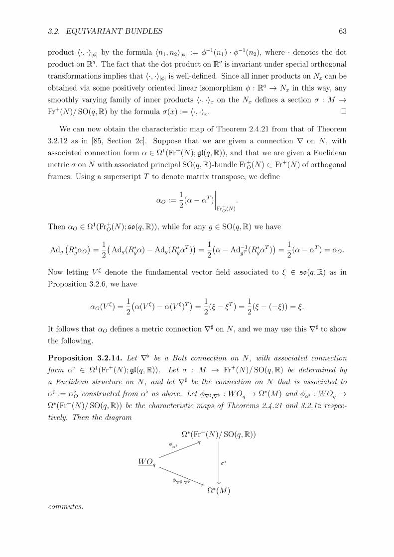
3.2. EQUIVARIANT BUNDLES 63
product 〈·, ·〉[φ] by the formula 〈n1, n2〉[φ] := φ−1(n1) · φ−1(n2), where · denotes the dot
product on Rq. The fact that the dot product on Rq is invariant under special orthogonal
transformations implies that 〈·, ·〉[φ] is well-defined. Since all inner products on Nx can be
obtained via some positively oriented linear isomorphism φ : Rq → Nx in this way, any
smoothly varying family of inner products 〈·, ·〉x on the Nx defines a section σ : M →Fr+(N)/ SO(q,R) by the formula σ(x) := 〈·, ·〉x.
We can now obtain the characteristic map of Theorem 2.4.21 from that of Theorem
3.2.12 as in [85, Section 2c]. Suppose that we are given a connection ∇ on N , with
associated connection form α ∈ Ω1(Fr+(N); gl(q,R)), and that we are given a Euclidean
metric σ on N with associated principal SO(q,R)-bundle Fr+O(N) ⊂ Fr+(N) of orthogonal
frames. Using a superscript T to denote matrix transpose, we define
αO :=1
2(α− αT )
∣∣∣∣Fr+O(N)
.
Then αO ∈ Ω1(Fr+O(N); so(q,R)), while for any g ∈ SO(q,R) we have
Adg(R∗gαO
)=
1
2
(Adg(R
∗gα)− Adg(R
∗gα
T ))
=1
2
(α− Ad−1
gT (R∗gαT ))
=1
2(α− αT ) = αO.
Now letting V ξ denote the fundamental vector field associated to ξ ∈ so(q,R) as in
Proposition 3.2.6, we have
αO(V ξ) =1
2
(α(V ξ)− α(V ξ)T
)=
1
2(ξ − ξT ) =
1
2(ξ − (−ξ)) = ξ.
It follows that αO defines a metric connection ∇] on N , and we may use this ∇] to show
the following.
Proposition 3.2.14. Let ∇[ be a Bott connection on N , with associated connection
form α[ ∈ Ω1(Fr+(N); gl(q,R)). Let σ : M → Fr+(N)/ SO(q,R) be determined by
a Euclidean structure on N , and let ∇] be the connection on N that is associated to
α] := α[O constructed from α[ as above. Let φ∇],∇[ : WOq → Ω∗(M) and φα[ : WOq →Ω∗(Fr+(N)/ SO(q,R)) be the characteristic maps of Theorems 2.4.21 and 3.2.12 respec-
tively. Then the diagram
Ω∗(Fr+(N)/ SO(q,R))
WOq
Ω∗(M)
σ∗
φα[
φ∇],∇[
commutes.

64 CHAPTER 3. HOLONOMY AND RELATED CONSTRUCTIONS
Proof. Note that if U is any open set in M over which one has an orthonormal frame
field s : U → Fr+(N), then letting p : Fr+(N)→ Fr+(N)/ SO(q,R) denote the projection
we have
(p s)(x) = class of the frame s(x) in Fr+(N)(x)/ SO(q,R) = σ(x).
The problem being local, it then suffices to show that in any local orthonormal frame s
over U ⊂ M , for any w ∈ WOq the form φα[(w)|U ∈ Ω(Fr+(N)|U/ SO(q,R)) pulls back
under p s : U → Fr+(N)|U to φ∇],∇[(w)|U ∈ Ω(U).
Fix such a U and s. The pullback under s of R[ is precisely the curvature R[U of ∇[
over U , so
s∗p∗φα[(ci) = s∗Tr((R[)i
)= Tr
((R[
U)i)
= φ∇],∇[(ci)|U
for all i, and it remains to show that for i odd we have s∗φα[(hi) = φ∇],∇[(hi)|U .
Write α[ = α[S + α[O = α[S + α], where α[S is the symmetric component of the matrix
α and α[O is the antisymmetric component. Then for any t ∈ [0, 1] we have
αt := (1− t)α] + tα[ = (1− t)α] + t(α[S + α]) = α] + tα[S
while in the notation of Theorem D.3.5, we have
Rt =dαt + αt ∧ αt=dα] + tdα[S +
(α] + tα[S
)∧(α] + tα[S
)=dα] +
((α])2 + (α[S)2
)+ t(dα[S + (α[Sα
] + α]α[S))
+ (t2 − 1)(α[S)2
=RO + tRS + (t2 − 1)(α[S)2,
using the equations (D.1) and (D.2) in going from the third line to the fourth. Now by
Theorem D.3.5, for i odd we have
s∗p∗φα[(hi) =is∗(
Tr
(∫ 1
0
α[S(RO + tRS + (t2 − 1)(α[S)2
)dt
))=is∗
(Tr
(∫ 1
0
(α[ − α])Rtdt
))=φ∇],∇[(hi)|U , .
since s∗α[ and s∗α] are the local connection forms corresponding to∇[ and∇] in the frame
s while s∗Rt is the curvature of (1−t)∇]+t∇[ in the frame s. Thus σ∗φα[ = φ∇],∇[ .
In fact the positively oriented frame bundle of N is just one example of a jet bundle
associated to N . We explore higher order jet bundles in the next subsection.

3.2. EQUIVARIANT BUNDLES 65
3.2.2 Jets and jet groups
The material we present in this subsection is adapted from [109, Section 13]. Roughly
speaking, the kth jet bundle of N encodes the transverse partial derivatives of total order
k of transverse coordinate maps for (M,F). Thus in particular, the positively oriented
frame bundle Fr+(N) of N , which encodes first order transverse partial derivatives of
sections of N , coincides with the first jet bundle J+1 (F) of N .
Let us be more precise. Recall that the positively oriented frame bundle Fr+(N)
consists, over any point x ∈M , of all positively oriented linear isomorphisms φ : Rq → Nx.
Fix x ∈ M . In a foliated chart about x, the normal bundle N can be regarded as the
tangent bundle TBt to an open rectangle Bt ⊂ Rq. Let us denote by x0 the image of
x in Bt under the transverse coordinate submersion defined by the foliated coordinates.
Then every positively oriented linear isomorphism φ : Rq → Tx0Bt can be identified with
the differential of some orientation-preserving local diffeomorphism ϕ of Rq sending 0 to
x0. That is,
φ = dϕ|0 : Rq → Tx0Bt.
Writing ϕ = (ϕ1, . . . , ϕq), we of course have the matrix representation
dϕ|0 =
(∂ϕi
∂zj
∣∣∣∣0
)i,j=1,...,q
.
Therefore if ϕ and ψ are two distinct orientation-preserving local diffeomorphisms that
send 0 to x0, which have the same first order partial derivatives, then they determine via
their differentials the same frame φ : Rq → Tx0Bt. It is routine to check that the relation
ϕ ∼ ψ if and only if∂ϕi
∂zj
∣∣∣∣0
=∂ψi
∂zj
∣∣∣∣0
for all i, j = 1, . . . , q
is an equivalence relation on orientation-preserving local diffeomorphisms of Rq sending
0 to x0, and we denote by j10(ϕ) the equivalence class under this equivalence relation
of any such orientation-preserving local diffeomorphism ϕ. More generally, we have the
following definition.
Definition 3.2.15. Let U and V be open subsets of Rq, and let x ∈ V . The relation
ϕ ∼k,x ψ if and only if∂|I|ϕi
∂zI
∣∣∣∣x
=∂|I|ψi
∂zI
∣∣∣∣x
for all I ∈ Zq+, |I| = i1 + · · ·+ iq ≤ k
defines an equivalence relation on orientation-preserving diffeomorphisms V → U . The
∼k,x-equivalence class of any such diffeomorphism ϕ is called the k-jet at x of ϕ, and is
denoted jkx(ϕ).

66 CHAPTER 3. HOLONOMY AND RELATED CONSTRUCTIONS
Moreover, the relation
ϕ ∼k ψ if and only if ϕ ∼k,x ψ for all x ∈ U
also defines an equivalence relation on orientation-preserving diffeomorphisms U → V .
The ∼k-equivalence class of any such diffeomorphism ϕ is called the k-jet of ϕ and is
denoted jk(ϕ).
A straightforward but tedious exercise using the multivariable chain rule shows that
k-jets of diffeomorphisms can be composed in a well-defined manner.
Proposition 3.2.16. Let U , V , W be open subsets of Rq and let ψ : W → V , ϕ : V → U
be diffeomorphisms. Then for each k ∈ N and each x ∈ W , the composition
jkψ(x)(ϕ) jkx(ψ) := jkx(ϕ ψ)
is well-defined and associative. Consequently, the composition of jk(ϕ) and jk(ψ) defined
by
jk(ϕ) jk(ψ) := jk(ϕ ψ)
is well-defined and associative.
Let us now turn to the special case of local diffeomorphisms ϕ of Rq that fix the origin.
Let G+k (q) denote the collection of k-jets at zero of all such local diffeomorphisms. Write
the k-jet at 0 of any such local diffeomorphism ϕ as the polynomial
jk0 (ϕ) =
( ∑1≤|I|≤k
∂|I|ϕi
∂zI
∣∣∣∣0
zI)i=1,...,q
(3.1)
in the variables [z1, . . . , zq]. The ϕiI := ∂|I|ϕi
∂zI
∣∣0
define coordinates on G+k (q) under which
G+k (q) is an open subset of Euclidean space [109, 13.1]. It is immediate from Proposition
3.2.16 that G+k (q) is a group under the composition of jets at 0 (the identity is given by
the k-jet at zero of the identity diffeomorphism of Rq), and it can be checked using the
multivariable chain rule that the composition of jets at 0 is polynomial in the coordinates
defined by (3.1). The following result is then immediate.
Proposition/Definition 3.2.17. The set
G+k (q) := jk0 (ϕ) : ϕ is a local diffeomorphism of Rq, ϕ(0) = 0,
equipped with the composition of k-jets, is a Lie group called the kth (positively ori-
ented) jet group of Rq. In particular, G+1 (q) identifies via the coordinates in (3.1) with
the positively oriented general linear group GL+(q,R).

3.2. EQUIVARIANT BUNDLES 67
We will be interested primarily in the groups G+2 (q) and G+
1 (q). Note that there is
a natural epimorphism π : G+2 (q)→ G+
1 (q) defined by forgetting second-order derivative
information. Thus, setting N 1 := ker(π) we have the exact sequence
id→ N 1 → G+2 (q)
π−→ G+1 (q)→ id .
In fact we have a canonical splitting i : G+1 (q) → G+
2 (q) of this exact sequence obtained
by sending a matrix A ∈ GL+(q,R) to the 2-jet of the linear diffeomorphism x 7→ Ax
on Rq. Let S2((Rq)∗) denote the second symmetric power of the dual (Rq)∗ of Rq, which
is the quotient of the second tensor power of (Rq)∗ by elements v ⊗ w − w ⊗ v. We see
then that GL+(q,R) acts on the space Rq⊗S2((Rq)∗) by taking it to act in the usual way
on the first factor and trivially on the second. Then the splitting i allows us to realise
G+2 (q) as the semidirect product (Rq⊗S2((Rq)∗)) o GL+(q,R). In particular, we have a
realisation
N 1 = id +Rq⊗S2(Rq) (3.2)
which will prove quite useful in what follows.
3.2.3 Jet bundles
We have already seen that associated to (M,F) is the principal GL+(q,R) = G+1 (q)-
bundle Fr+(N) of positively oriented frames of N , which encodes first order transverse
derivative information. In order to capture higher order transverse derivatives (such as
those coming from curvature), we need to introduce transverse jet bundles for (M,F), of
which Fr+(N) is just the easiest example. The material presented in this subsection is
adapted from [108, 25, 24, 154, 124].
Construction 3.2.18. Take a regular foliated atlas U = (Uα, xα, yα))α∈A for (M,F),
where xα : Uα → Bατ ⊂ Rp and yα : Uα → Bα
t ⊂ Rq are submersions defining plaques
and local transversals respectively. Recall (see Definition 2.2.8) that associated to U is a
collection cαβα,β∈A of diffeomorphisms cαβ : yβ(Uα ∩ Uβ) → yα(Uα ∩ Uβ) satisfying the
cocycle condition
cαδ = cαβ cβδ
on yδ(Uα ∩ Uβ ∩ Uδ) for all α, β, δ ∈ A.
Now over each of the open rectangles Bαt ⊂ Rq and for each k ≥ 0, one can associate
a space J+k (α) by fixing an open rectangle U 3 0 in Rq and defining
J+k (α) := jk0 (ϕ) : ϕ : U → Bα
t is a diffeomorphism.
Equipped with the projection πk : J+k (α)→ Bα
t defined by πk(jk0 (ϕ)) := ϕ(0), we obtain

68 CHAPTER 3. HOLONOMY AND RELATED CONSTRUCTIONS
a trivialisation J+k (α) ∼= Bα
t ×G+k (q) defined by
jk0 (ϕ) 7→(ϕ(0), jk0 (ϕ tϕ(0))
),
where tϕ(0) : y 7→ y − ϕ(0) is translation. Thus J+k (α) is a trivial principal G+
k (q)-bundle
over Bαt and moreover does not depend on the neighbourhood U of 0 ∈ Rq which we used
to define it.
We form the pullbacks y∗α(J+k (α)) over Uα for each α. We then set
J+k (F) :=
( ⊔α∈A
y∗α(J+k (α))
)/ ∼, (3.3)
where ∼ is the equivalence relation defined by
(α, x, jk0 (ϕ)) ∼ (β, x, jk0 (ψ)) if and only if x ∈ Uα ∩ Uβ 6= ∅ and jk0 (ϕ) = jk0 (cαβ ψ).
We let πk : J+k (F)→ M be defined by the obvious map [(α, x, jk0 (ϕ))] 7→ x, and observe
that by construction J+k (F) is isomorphic over each Uα to Uα×G+
k (q). Then πk : J+k (F)→
M is a principal G+k (q)-bundle over M , which by construction encodes the kth-order
transverse derivative information associated to (M,F). In particular, J+1 (F) coincides
with the positively oriented transverse frame bundle Fr+(N).
Definition 3.2.19. The principal G+k (q)-bundle πk : J+
k (F)→M is called the positively
oriented transverse k-jet bundle of (M,F).
In fact for each k ≥ 1, J+k+1(F) is a bundle over J+
k (F) with projection that we denote
πk+1,k : J+k+1(F)→ J+
k (F). The transverse k-jet bundles are G-spaces.
Construction 3.2.20. Over a point x ∈ M , contained in a foliated chart Bατ × Bα
t ,
the fibre J+k (F)x is the space of k-jets jk0 (ϕ) defined for orientation-preserving diffeomor-
phisms ϕ : U → Bαt such that ϕ(0) = x. If u ∈ Gx, then u can be represented by a
diffeomorphism h of a sufficiently small open neighbourhood of x = ϕ(0) in Bαt onto an
open neighbourhood of the local transversal Bβt containing r(u). The formula
uk · jk0 (ϕ) := jk0 (h ϕ) ∈ J+k (F)r(u)
is well-defined since two diffeomorphisms with the same germ at a point have the same
k-jets at that point, and determines an action G ×s,πkJ+k (F) 3 (u, jk0 (ϕ)) 7→ uk · jk0 (ϕ) ∈
J+k (F). Now by Proposition 3.2.2, we know that the πk : J+
k (F)→M are G-bundles, and
in particular the projections πk are equivariant with respect to the action of G. Moreover
since πk πk+1,k = πk+1 for all k, inductively we see that πk+1,k : J+k+1(F) → J+
k (F)
defines J+k+1(F) as a G-bundle over J+
k (F), so that each πk+1,k is also equivariant and
maps T Fk+1 to T Fk.
3.2. EQUIVARIANT BUNDLES 69
Definition 3.2.21. We denote by Fk the foliation of J+k (F) induced as in Construc-
tion 3.2.20, and denote by Nk := TJ+k (F)/T Fk and Gk = GnJ+
k (F) the corresponding
normal bundle and holonomy groupoid respectively. Let πNk : Nk → J+k (F) denote the
projection for the normal bundle. Then the action
G ×s,πkJ+k (F) 3 (u, jk0 (ϕ)) 7→ uk · jk0 (ϕ) ∈ Jk0 (F)
of G on J+k (F) induces a corresponding action
G ×s,πkπNkNk 3 (u, nk) 7→ uk∗nk ∈ Nk
on the normal bundle Nk by Proposition 3.2.1.
We will see shortly how the structure of the bundles J+2 (F) and J+
1 (F) encode all the
information required to derive the usual connection and curvature formalism that one
obtains on Fr+(N) from connections on the normal bundle N . Philosophically speaking,
this is not very surprising: J+2 (F) encodes all second order transverse derivative infor-
mation, and a connection on N specifies how to perform a first order derivative of a
transverse vector field. On a technical level, one obtains the connection formalism from
tautological forms on J+2 (F), first laid out by Kobayashi [108], which we now discuss.
Recall from Definition 2.3.2 that a transverse differential form on a foliated manifold
is a form which vanishes whenever any one of its inputs is a leafwise vector field.
Definition 3.2.22. By abuse of notation let dπ1 : N1 → N denote the vector bundle map
induced by π1 : J+1 (F) → M . The solder form is the canonical Rq-valued transverse
1-form θ1 : N1 → Rq on J+1 (F) defined by
θ1j10(ϕ)(X) := (dϕ−1 dπ1)j10(ϕ)(X), j1
0(ϕ) ∈ J1+(F), X ∈ (N1)j10(ϕ).
The solder form is well-defined because dϕ−1 is determined by j10(ϕ) = dϕ.
The solder form associated to the frame bundle of a manifold is of course well-known,
and the definition we give above is just its natural generalisation to the transverse geome-
try of a foliation. The vector θ1j10(ϕ)
(X) ∈ Rq is essentially the expression of the horizontal
part of X ∈ N1 in the frame j10(ϕ). As we will soon see, we can obtain a tautological
form θk on any higher order bundle J+k (F) in an analogous way.
Definition 3.2.23. Fix an open ball U 3 0 in Rq, and let J+k (Rq) denote the bundle
J+k (Rq) := jk0 (ψ) : ψ : U → Rq is a local diffeomorphism

70 CHAPTER 3. HOLONOMY AND RELATED CONSTRUCTIONS
over Rq, with projection J+k (Rq) 3 jk0 (ψ) 7→ ψ(0) ∈ Rq. We denote
jk(q) := Tjk0 (id)J+k (Rq),
where id : U → Rq is the identity map.
Essentially the jk(q) capture the infinitesimal structure of higher order frames. Note
in particular that J+0 (Rq) is just Rq, hence j0(q) = Rq. The solder form can then be
viewed in this light as a map N1 → j0(q), which lends itself easily to generalisation.
Construction 3.2.24. Let k ≥ 1. Let U be an open neighbourhood of 0 ∈ Rq,
(Uα, xα, yα) a foliated chart in M , and let ϕ : U → yα(Uα) be a local diffeomorphism.
Suppose that Z ∈ jk−1(q). Then we can choose a family ψt : U → Rq of local diffeomor-
phisms, parameterised by t ∈ (−ε, ε), such that ψ0 = id : U → Rq and
Z =d
dt
∣∣∣∣t=0
jk−10 (ψt).
Now by choosing ε sufficiently small, the composition ϕ ψt makes sense for all t and we
obtain a map djk−1(ϕ) : jk−1(q)→ (Nk)jk−1(ϕ) defined by
djk−1(ϕ)(Z) =d
dt
∣∣∣∣t=0
jk−10 (ϕ ψt).
The map djk−1(ϕ) is an isomorphism by dimension count and depends only on jk0 (ϕ).
Moreover dj0(ϕ) is equal to dϕ : Rq → N .
Definition 3.2.25. By abuse of notation, let dπk,k−1 : Nk → Nk−1 denote the projection
induced by the map πk,k−1 : J+k (F)→ J+
k−1(F). The tautological form of degree k is
the jk−1(q)-valued transverse 1-form θk : Nk → jk−1(q) defined by
θkjk0 (ϕ)(X) := (djk−1(ϕ)−1 dπk,k−1)jk0 (ϕ)(X), jk0 (ϕ) ∈ J+k (F), X ∈ (Nk)jk0 (ϕ).
The form θk is well-defined on J+k (F), because djk−1(ϕ) depends only on jk0 (ϕ).
In close analogy with the solder form θ1, for X ∈ (Nk)jk0 (ϕ), the quantity θkjk0 (ϕ)
(X)
is the expression of the normal vector X in the higher order frame jk0 (ϕ). Crucially, the
tautological forms are invariant under the action of G on the transverse jet bundles.
Proposition 3.2.26. For all u ∈ G and jk0 (ϕ) with ϕ(0) = s(u), we have
((uk)∗θk
)jk0 (ϕ)
= θkjk0 (ϕ).
Thus θk is invariant under the action of G.

3.2. EQUIVARIANT BUNDLES 71
Proof. Fix X ∈ (Nk)jk0 (ϕ). Then we calculate
((uk)∗θ
)jk0 (ϕ)
(X) =θkuk·jk0 (ϕ)(uk∗X)
=(d(uk−1 · jk−1(ϕ))−1
uk−1·jk−10 (ϕ)
dπk,k−1 uk∗)(X)
=(djk−1(ϕ)−1
jk−10 (ϕ)
(u−1)k−1∗ uk−1
∗ dπk,k−1
)(X)
=(djk−1(ϕ)−1
jk−10 (ϕ)
dπk,k−1
)(X)
=θkjk0 (ϕ)(X).
In going from the second line to the third we have implicitly represented u by a diffeo-
morphism h of local transversals about the range and source of u, so that uk−1 ·jk−1(ϕ) =
jk−1(h ϕ), hence by the chain rule
djk−1(h ϕ) = d(jk−1(h) jk−1(ϕ)) = uk−1∗ djk−1(ϕ).
We have also used that πk,k−1 is equivariant with respect to the action of G as in Con-
struction 3.2.20.
For computations in coordinates, we need to write θk in terms of a basis for jk−1(q).
Ultimately this will allow us to isolate a component of θ2 which defines a connection on the
differential graded algebra of forms on J+2 (F), from which we can define a characteristic
map that encodes the secondary class data already explored in Theorems 2.4.21 and
3.2.12.
Construction 3.2.27. Let k ≥ 1. The standard basis (e1, . . . , eq) in Rq gives us canonical
coordinates for J+k−1(Rq). More specifically, if U is an open neighbourhood of 0 in Rq,
then the k− 1-jet of any local diffeomorphism ψ =∑q
i=1 ψiei : U → Rq, is determined by
the sum
jk−10 (ψ) =
q∑i=1
(ψi(0) +
∑j
∂ψi
∂yj(0)yj + · · ·+
∑j1,...,jk−1
∂j1+···+jk−1ψi
∂yj1 · · · ∂yjk−1(0)yj1 · · · yjk−1
)ei.
For notational simplicity, we use multi-index notation J = (j1, . . . , jl), |J | = j1 + · · ·+ jl,
and substitute siJ for the partial derivative ∂|J|ψi
∂yJ(0). Then the siJ determine coordinates
for J+k−1(Rq), with respect to which the tangent vectors
∂Ji :=∂
∂siJ, i = 1, . . . , q, |J | ≤ k − 1
form a basis for jk−1(q). With respect to this basis, the tautological form θk on J+k (F)
72 CHAPTER 3. HOLONOMY AND RELATED CONSTRUCTIONS
can be written
θk =∑i
ωi∂i +∑i,j
ωij∂ji + · · ·+
∑i,|J |=k−1
ωiJ∂Ji ,
where the ωiJ are transverse 1-forms Nk → R on J+k (F).
Let us examine the structure of the forms ωiJ . Fix k and fix any multi-index J
with |J | ≤ k − 1. Let U be an open neighbourhood of 0 ∈ Rq, (Uα, xα, yα) a foliated
chart for (M,F) and consider jk0 (ϕ) ∈ J+k (F) defined for some local diffeomorphism
ϕ : U → yα(Uα). If X ∈ (Nk)jk0 (ϕ), we let ϕt : U → yα(Uα) be a family of local
diffeomorphisms, parameterised by t ∈ (−ε, ε), such that ϕ0 = ϕ and for which X is
represented as
X =d
dt
∣∣∣∣t=0
jk0 (ϕt).
Then we know that θk acts on X by the formula
θkjk0 (ϕ)(X) =d
dt
∣∣∣∣t=0
jk−10 (ϕ−1 ϕt).
Define x : U × (−ε, ε)→ U by x(y, t) := ϕ−1 ϕt(y), and using the standard coordinates
yi in U write
x(y, t) = (x1(y, t), . . . , xq(y, t)), (y, t) ∈ U × (−ε, ε).
Then for each t we can write
jk−10 (ϕ−1 ϕt) =
q∑i=1
(xi(0, t) +
∑j
∂xi
∂yj(0, t)yj + · · ·+
∑|J |=k−1
∂|J |xi
∂yJ(0, t)yJ
)ei
where ei denotes the ith standard basis vector in Rq. By commutativity of partial deriva-
tives we see therefore that
ωiJ(X) =∂
∂t
∣∣∣∣t=0
(∂|J |xi
∂yJ
∣∣∣∣y=0
)=∂|J |
∂yJ
∣∣∣∣y=0
(∂xi
∂t
∣∣∣∣t=0
). (3.4)
Note that because ωiJ depends only on the |J |+1-jet over which it sits, its pullback to all
higher order jet bundles makes sense and continues to compute the same quantity. We
will use the single symbol ωiJ to denote both ωiJ on J+|J |+1(F) as well as its pullbacks to
all the higher order jet bundles.
Associated to the forms ωiJ are the following structure equations. We need these
equations only up to |J | = 2, although analogous formulae are known for arbitrary |J |.

3.2. EQUIVARIANT BUNDLES 73
Proposition 3.2.28. For k ≥ 2, on J+k (F) we have
dωi = −ωij ∧ ωj (3.5)
while for k ≥ 3, on J+k (F) we have
dωij = −ωik ∧ ωkj − ωijk ∧ ωk. (3.6)
Here we have adopted the usual Einstein summation notation.
Proof. The result is well-known when F is a foliation by points [124, Proposition 3.23]. A
subtlety that is not recognised in the literature is that the same argument holds when F is
a general foliation only if we can show that the exterior derivatives of the transverse dif-
ferential forms ωi and ωij are again transverse differential forms. Since all the tautological
forms are G-invariant by Proposition 3.2.26, it suffices to show that if ω is a transverse
differential 1-form on a foliated manifold (M,F) that is invariant under the action of
its holonomy groupoid G, then dω is again a transverse differential form. That is, we
must show that the contraction ιXdω of dω by any leafwise vector field X ∈ Γ∞(M ;T F)
vanishes. For such X, and for Z ∈ Γ∞(M ;N), we compute
(ιXdω)(Z) = Xω(Z)− Zω(X)− ω([X,Z]) = Xω(Z)− ω(∇[XZ)
where ∇[ is any Bott connection on N . Thus we must show that Xω(Z) = ω(∇[XZ). Fix
x ∈M , and suppose that Xx = ddt
∣∣t=0γ(t) for some smooth curve γ in the leaf L through
x. Let P (γ)t : Nγ(0) → Nγ(t) denote the parallel transport along γ defined by the Bott
connection ∇[. Then we have
(∇[XZ)x
= limt→0
P (γ)−1t Zγ(t) − Zγ(0)
t.
Letting ut denote the element of G determined by the path γt(s) := γ(ts) in L, by
Proposition 3.2.5 we have P (γ)t = (ut)∗, and then the G-invariance of ω tells us that
ω(∇[XZ)x = lim
t→0
1
t
(ωγ0(P (γ)−1
t Zγ(t))− ωγ(0)
)= lim
t→0
1
t
(((u−1
t )∗ω)γ(t)(Zγ(t))− ωγ(0)(Zγ(0)))
= limt→0
1
t
(ωγ(t)(Zγ(t))− ωγ(0)(Zγ(0))
)=(Xω(Z)
)x
as required.
Note that Equation (3.5) is exactly what we would expect if the ωij assembled into
a torsion-free connection form ω := (ωij)i,j=1,...,q for N . Moreover rearranging Equation

74 CHAPTER 3. HOLONOMY AND RELATED CONSTRUCTIONS
(3.6) gives a formula suggestive of the curvature form of ω. In fact this resemblance
between the ω and the components of a connection form is quite deep, as the next two
results show.
Lemma 3.2.29. Let Rg denote the right action of g ∈ GL+(q,R) = G+1 (q) on J+
2 (F),
and for ξ ∈ gl(q,R) let V ξ denote the associated fundamental vector field on J+2 (F) as in
Proposition 3.2.6. The tautological gl(q,R)-valued form ω := (ωij)i,j=1,...,q satisfies
1. Adg(R∗gω
)= ω for all g ∈ GL+(q,R), and
2. ω(V ξ) = ξ for all ξ ∈ gl(q,R).
Proof. For the first part, fix X = ddt
∣∣t=0j2
0(ϕt) ∈ Tj20(ϕ)J+2 (F), where in the notation of
Construction 3.2.27 ϕt : U → yα(Uα) is a family of local diffeomorphisms with ϕ := ϕ0.
Then for g = j10(ϕ) ∈ GL+(q,R) = G+
1 (q), writing Rg for the right action of g on J+2 (F)
and adopting the usual Einstein summation convention, we have
(R∗gω
ij
)(X) =ωij(dRgX)
=∂
∂yj
(∂(ϕ−1 ϕ−1 ϕt ϕ)i
∂t
)∣∣∣∣0
=∂(ϕ−1)i
∂yk
∣∣∣∣0
∂
∂yl
(∂(ϕ−1 ϕt)k
∂t
)∣∣∣∣0
∂ϕl
∂yj
∣∣∣∣0
=(
Adg−1 ω)ij(X),
so that Adg(R∗gω
)= ω.
For the second part, fix ξ ∈ gl(q,R) = T1G+1 (q). Let ψt : U → U be a family of local
diffeomorphisms fixing 0 such that j20(ψt) = j1
0(ψt), for which ξ can be represented as the
tangent vector
ξ =d
dt
∣∣∣∣t=0
j10(ψt) =
(∂
∂yj
(∂ψit∂t
)∣∣∣∣0
)i,j=1,...,q
.
The fundamental vector field V ξ corresponding to ξ can then be written
V ξj2(ϕ) :=
d
dt
∣∣∣∣t=0
(j2
0(ϕ) · exp(tξ))
=d
dt
∣∣∣∣t=0
(j2
0(ϕ) · j10(ψt)
), j2
0(ϕ) ∈ J+2 (F).
Consequently, we see that
ωij(V ξ
j20(ϕ)
)=
∂
∂yj
(∂(ϕ−1 ϕ ψt)i
∂t
)∣∣∣∣0
=∂
∂yj
(∂ψit∂t
)∣∣∣∣0
= ξij, j20(ϕ) ∈ J+
2 (F).
Lemma 3.2.29 says that the tautological form ω behaves as though it is a connection
form on a principal GL+(q,R)-bundle, while as we have already observed Equation (3.5)
implies that this “connection form” is torsion-free. The next result formalises this ob-

3.2. EQUIVARIANT BUNDLES 75
servation: in its “non-foliated” form it is due to Kobayashi [108], while the relationship
with Bott connections does not appear in the literature.
Proposition 3.2.30. A choice of torsion-free connection ∇ on N is equivalent to a
choice of GL+(q,R)-equivariant section σ : J+1 (F)→ J+
2 (F). In particular, if ∇ = ∇[ is
a torsion-free Bott connection on N then the differential of σ restricts to a map T F1 →T F2 of the leafwise tangent bundles of J+
1 (F) and J+2 (F) respectively.
Proof. If we are gifted a GL+(q,R)-equivariant section σ : J+1 (F) → J+
2 (F), then
Lemma 3.2.29 together with Equation (3.5) of Proposition 3.2.28 guarantees that σ∗ω ∈Ω1(J+
1 (F); gl(q,R)) is the connection form of a torsion-free connection ∇ on N . Suppose
on the other hand that we are gifted a torsion-free connection∇ on N . Following the ideas
of [60], ∇ determines a torsion-free affine connection on any local transversal Yx through
any point x ∈ M , and is therefore associated with an exponential map exp∇x which pro-
vides a diffeomorphism of some open neighbourhood V of 0 ∈ Nx∼= Tx Yx onto an open
neighbourhood U of x in Yx. Then given a frame φ ∈ Fr+(N)x = J+1 (F)x, thought of as
a linear isomorphism Rq → Nx, we define the open neighbourhood W := φ−1(V ) of 0 in
Rq and observe that the composition
ϕφ := exp∇x φ|W
defines a diffeomorphism of W ⊂ Rq onto U ⊂ Yx. We now obtain a section σ : J+1 (F)→
J+2 (F) by the formula
σ(φ) := j20(ϕφ), φ ∈ J+
1 (F).
To see that σ is GL+(q,R)-equivariant, suppose that g ∈ GL+(q,R). Then g is a linear
diffeomorphism of Rq fixing 0 and for φ ∈ J+1 (F) we have ϕφ·g = exp∇x φg. Consequently
we see that
σ(φ · g) = j20(ϕφ·g) = j2
0(ϕφ g) = σ(φ) · g
so that σ is equivariant.
For the second part, observe that the construction of ω guarantees that it vanishes
on Γ∞(J+2 (F); ker(dπ2,1) ⊕ T F2), while the connection form α[ ∈ Ω1(J+
1 (F); gl(q,R))
associated to any Bott connection vanishes on Γ∞(J+1 (F);T F1) by Proposition 3.2.9.
Then the formula σ∗ω = α implies that dσ : T F1 → ker(dπ2,1) ⊕ T F2. Since dσ is
fibrewise linear, the subbundle dσ(T F1) of ker(dπ2,1)⊕ T F2 has rank at most dim(F).
Then the fact that dπ2,1 restricts to a fibrewise isomorphism T F2 → T F1 together with
the fact that σ is a section of π2,1 together imply that dσ maps T F1 into T F2.
Now the principal G+2 (q)-bundle J+
2 (F) over M carries in particular a right action of
GL+(q,R) = G+1 (q) ⊂ G+
2 (q). Consequently, in a similar manner to what we saw in Con-
struction 3.2.11, the algebra Ω∗(J+2 (F)) can be taken as a GL+(q,R)-differential graded

76 CHAPTER 3. HOLONOMY AND RELATED CONSTRUCTIONS
algebra, whose SO(q,R)-basic elements identify with Ω∗(J+2 (F)/ SO(q,R)). Moreover,
the properties of ω exhibited in Proposition 3.2.30 imply that ω is a connection for the
GL+(q,R)-differential graded algebra Ω(J+2 (F)) in the sense of Definition D.2.8. Recall-
ing the definition of WOq (Definition 2.4.10) and its truncated version WOq (Definition
2.4.19) we have the following characteristic map.
Theorem 3.2.31. There is a canonical homomorphism φ : WOq → Ω∗(J+2 (F)/ SO(q,R))
of differential graded algebras.
Proof. We obtain a homomorphism φ : WOq → Ω∗(J+2 (F)/ SO(q,R)) in the same way
as in Theorem 3.2.12, by mapping the canonical connection form for W (gl(q,R)) to the
components of the tautological connection form ω on J+2 (F). Let Ω := dω + ω ∧ ω
denote the tautological curvature form associated to ω. Then the elements ci ∈ I∗q (R) =
R[c1, . . . , cq] ⊂ WOq are mapped by φ to the form on J+2 (F)/ SO(q,R) determined by
Tr(Ωi).
We need only show now that φ : WOq → Ω∗(J+2 (F)/ SO(q,R)) descends to a homo-
morphism WOq → Ω∗(J+2 (F)/ SO(q,R)). Let Ω = π∗3,2Ω denote the copy of Ω on J+
3 (F),
where π3,2 : J+3 (F)→ J+
2 (F) is the projection. By Equation (3.6) we have
Ωij = −
q∑k=1
ωijk ∧ ωk.
Since there are only q distinct ωk’s we see that any monomial of degree greater than q
in the components of Ω on J+3 (F) must vanish (this fact can be seen as a form of Bott’s
vanishing theorem, Theorem 2.4.18). A choice of section s : J+2 (F) → J+
3 (F) gives
s∗Ω = s∗π∗3,2Ω = Ω, from which we deduce that any monomial of degree greater than q
in the components of Ω on J+2 (F) must vanish also. Consequently any monomial of total
degree greater than 2q in the φ(ci) must also vanish, which implies that φ descends to a
homomorphism WOq → Ω∗(J+2 (F)/ SO(q,R)) as claimed.
The following result relating the characteristic maps of Theorems 3.2.31, 3.2.12 and
2.4.21 is now an immediate corollary of Proposition 3.2.30.
Corollary 3.2.32. Let ∇[ be a torsion-free Bott connection on N with associated con-
nection form α[ on J+1 (F), and with associated section σ2 : J+
1 (F) → J+2 (F). Let
σ1 : M → J+1 (F)/ SO(q,R) be determined by a Euclidean structure on N , and let
∇] be the metric compatible connection on N obtained from σ1 and α[ as in Proposi-
tion 3.2.14. Let φ∇],∇[ : WOq → Ω∗(M), φα[ : WOq → Ω∗(J+1 (F)/ SO(q,R)), and
φ : WOq → Ω∗(J+2 (F)/ SO(q,R)) be the characteristic maps of Theorems 2.4.21, 3.2.12
and 3.2.31 respectively. Then the diagram
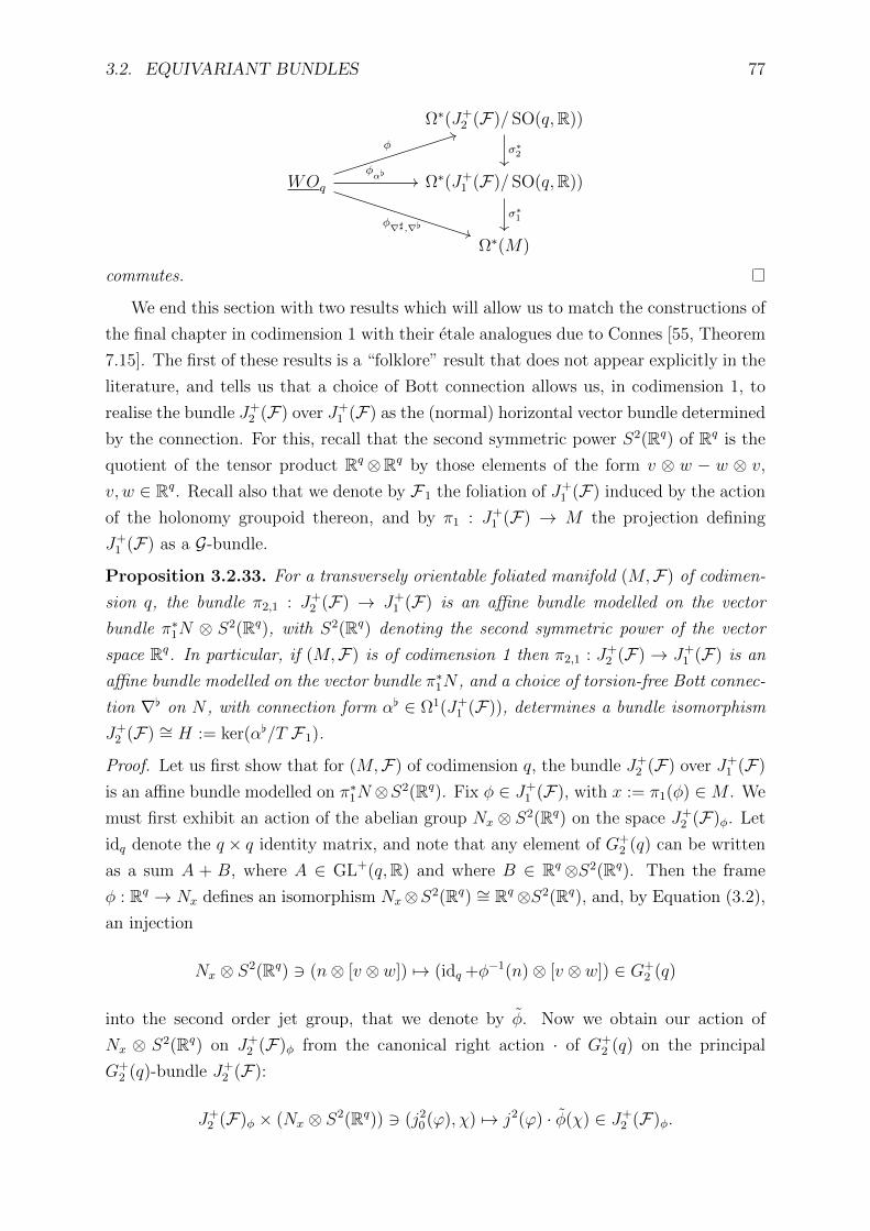
3.2. EQUIVARIANT BUNDLES 77
Ω∗(J+2 (F)/ SO(q,R))
WOq Ω∗(J+1 (F)/ SO(q,R))
Ω∗(M)
σ∗2φ
φα[
φ∇],∇[σ∗1
commutes.
We end this section with two results which will allow us to match the constructions of
the final chapter in codimension 1 with their etale analogues due to Connes [55, Theorem
7.15]. The first of these results is a “folklore” result that does not appear explicitly in the
literature, and tells us that a choice of Bott connection allows us, in codimension 1, to
realise the bundle J+2 (F) over J+
1 (F) as the (normal) horizontal vector bundle determined
by the connection. For this, recall that the second symmetric power S2(Rq) of Rq is the
quotient of the tensor product Rq⊗Rq by those elements of the form v ⊗ w − w ⊗ v,
v, w ∈ Rq. Recall also that we denote by F1 the foliation of J+1 (F) induced by the action
of the holonomy groupoid thereon, and by π1 : J+1 (F) → M the projection defining
J+1 (F) as a G-bundle.
Proposition 3.2.33. For a transversely orientable foliated manifold (M,F) of codimen-
sion q, the bundle π2,1 : J+2 (F) → J+
1 (F) is an affine bundle modelled on the vector
bundle π∗1N ⊗ S2(Rq), with S2(Rq) denoting the second symmetric power of the vector
space Rq. In particular, if (M,F) is of codimension 1 then π2,1 : J+2 (F)→ J+
1 (F) is an
affine bundle modelled on the vector bundle π∗1N , and a choice of torsion-free Bott connec-
tion ∇[ on N , with connection form α[ ∈ Ω1(J+1 (F)), determines a bundle isomorphism
J+2 (F) ∼= H := ker(α[/T F1).
Proof. Let us first show that for (M,F) of codimension q, the bundle J+2 (F) over J+
1 (F)
is an affine bundle modelled on π∗1N⊗S2(Rq). Fix φ ∈ J+1 (F), with x := π1(φ) ∈M . We
must first exhibit an action of the abelian group Nx ⊗ S2(Rq) on the space J+2 (F)φ. Let
idq denote the q × q identity matrix, and note that any element of G+2 (q) can be written
as a sum A + B, where A ∈ GL+(q,R) and where B ∈ Rq⊗S2(Rq). Then the frame
φ : Rq → Nx defines an isomorphism Nx⊗S2(Rq) ∼= Rq⊗S2(Rq), and, by Equation (3.2),
an injection
Nx ⊗ S2(Rq) 3 (n⊗ [v ⊗ w]) 7→ (idq +φ−1(n)⊗ [v ⊗ w]) ∈ G+2 (q)
into the second order jet group, that we denote by φ. Now we obtain our action of
Nx ⊗ S2(Rq) on J+2 (F)φ from the canonical right action · of G+
2 (q) on the principal
G+2 (q)-bundle J+
2 (F):
J+2 (F)φ × (Nx ⊗ S2(Rq)) 3 (j2
0(ϕ), χ) 7→ j2(ϕ) · φ(χ) ∈ J+2 (F)φ.

78 CHAPTER 3. HOLONOMY AND RELATED CONSTRUCTIONS
Thus J+2 (F)φ is an affine space modelled on the vector space Nx ⊗ S2(Rq).
To finish the proof that π2,1 : J+2 (F) → J+
1 (F) is an affine bundle we need only
show that we can gift it with an atlas of local trivialisations whose transition functions
are affine isomorphisms. However by construction (see Construction 3.2.18), the J+k (F)
are obtained from gluing together the (canonically trivial) local jet bundles y∗α(J+k (α))
associated to a regular foliated atlas (Uα, xα, yα)α∈A. Define N 1 to be the kernel of
the canonical homomorphism G+2 (q) → G+
1 (q) obtained by forgetting the second order
derivatives, and for each α ∈ A, define U1α to be the image of y∗α(J+
1 (α)) in J+1 (F). Then
J+2 (F)|U1
α∼= y∗α(J+
2 (α)) ∼= U1α × N 1. Now suppose that φ ∈ U1
β ∩ U1α, and consider any
element (φ,
(∂2ϕi
∂yj∂yk
∣∣∣∣0
)ijk
)∈ U1
β ×N 1,
where ϕ is a diffeomorphism from a neighbourhood of 0 ∈ Rq to yβ(Uβ) such that [j10(ϕ)] =
φ. Let cαβ : yβ(Uα ∩ Uβ) → yα(Uα ∩ Uβ) be the diffeomorphism obtained from the
transverse change of coordinates. Letting (y1, . . . , yq) denote the standard coordinates in
Rq, we use the chain rule to compute
j20(cαβ ϕ) =
(∂ciαβ∂yl
∣∣∣∣ϕ(0)
∂ϕl
∂yj
∣∣∣∣0
)ij
+
(∂2ciαβ∂yj∂yl
∣∣∣∣ϕ(0)
∂ϕl
∂yk
∣∣∣∣0
+∂ciαβ∂yl
∣∣∣∣ϕ(0)
∂2ϕl
∂yj∂yk
∣∣∣∣0
)ijk
,
where we use the usual Einstein summation convention. Defining ρil(φ) :=∂ciαβ∂yl
∣∣ϕ(0)
and ρijk(φ) :=∂2ciαβ∂yj∂yl
∣∣ϕ(0)
∂ϕl
∂yk
∣∣0
we see that our transition function (U1α ∩ U1
β) × N 1 →(U1
α ∩ U1β)×N 1 is the affine transformation given by
(φ,
(∂2ϕi
∂yj∂yk
∣∣∣∣0
)ijk
)7→(φ,
(ρil(φ)
∂2ϕi
∂yj∂yk
∣∣∣∣0
+ ρijk(φ)
)ijk
).
This completes the proof that π2,1 : J+2 (F)→ J+
1 (F) is an affine bundle.
The second part is now easy. When q = 1, multiplication in R gives S2(R) ∼= Rand then π∗1N ⊗ S2(R) ∼= π∗1N . As we have already seen in Proposition 3.2.10, if α[ ∈Ω1(J+
1 (F)) is the connection form of a torsion-free Bott connection ∇[ on N , then the
quotient H := ker(α[)/T F1 is isomorphic to π∗1N . By Proposition 3.2.30, ∇[ determines
a section σ[ of the affine bundle J+2 (F)→ J+
1 (F), and therefore an identification of J+2 (F)
with the vector bundle π∗1N on which it is modelled. Consequently, J+2 (F) identifies with
H as claimed.
The second and final result we will need is an explicit representative of the codimension
1 Godbillon-Vey class on J+2 (F) (or rather on the horizontal normal bundle determined
by a Bott connection as in Proposition 3.2.33). An etale version of this result has been
known for decades [55], although it is difficult to find a proof in the literature so we give

3.2. EQUIVARIANT BUNDLES 79
a full proof below.
Proposition 3.2.34. Let (M,F) be a transversely orientable foliation of codimension 1,
with transverse volume form ω ∈ Ω1(M). Suppose moreover we have a torsion-free Bott
connection on N determining an identification J+2 (F) = H/T F1 as in Proposition 3.2.33.
The form ω gives rise to a trivialisation H/T F1 = M×R∗+×R, with coordinates (x, t, h).
With respect to these coordinates the Godbillon-Vey class on H/T F1 is represented by
the G-invariant differential form
gv = − 1
t3ω ∧ dt ∧ dh.
Proof. Let (ω0, ω1, ω2) denote the tautological form on J+3 (F), so that ω0 is the solder
form on J+1 (F), ω1 is the tautological connection form on J+
2 (F), and by the structure
equations of Proposition 3.2.28 we have dω1 = ω0∧ω2 on J+3 (F). Under the characteristic
map φ : WOq → Ω∗(J+2 (F)) of Theorem 3.2.31, the Godbillon-Vey class is represented
by the G-invariant form
φ(h1c1) = ω1 ∧ dω1 = −ω0 ∧ ω1 ∧ ω2
on J+3 (F). We will give an expression for this form in coordinates, showing in particular
that it resides naturally on J+2 (F) and has the form of Equation (3.2.34).
Associated to the transverse volume form ω is a nonvanishing normal vector field
Z ∈ Γ∞(M ;N) characterised by the equation ω(Z) ≡ 1. Fix x ∈M and let Yx be a local
transversal through x. Then the torsion-free Bott connection ∇[ on N restricts to an
affine connection on Yx, and so determines an exponential map exp∇[
: U → Yx which is
a local diffeomorphism defined on an open neighbourhood U of 0 ∈ Tx Yx. Rescaling ω if
necessary, we can always assume that Zx ∈ U and we obtain a coordinate u0 : Yx → Rdefined by the equation
u0(x′)Zx =(
exp∇[ )−1
(x′), x′ ∈ Yx .
Now fix a local diffeomorphism ϕ from an open neighbourhood of 0 ∈ R to Yx. The
coordinate u0 on Yx identifies ϕ with a local diffeomorphism ϕ := u0 ϕ of R, so the 3-jet
j30(ϕ) is determined by the polynomial
ϕ(0) +dϕ
dy
∣∣∣∣0
y +d2ϕ
dy2
∣∣∣∣0
y2 +d3ϕ
dy3
∣∣∣∣0
y3
where we use y to denote the standard coordinate in R. We thus define coordinates
ui(j30(ϕ)) := diϕ
dyi
∣∣0
for i = 1, 2, 3 for j30(ϕ) ∈ J+
3 (Yx). Suppose now that ϕt is a 1-
parameter family of local diffeomorphisms from an open neighbourhood of 0 ∈ R to Yx,
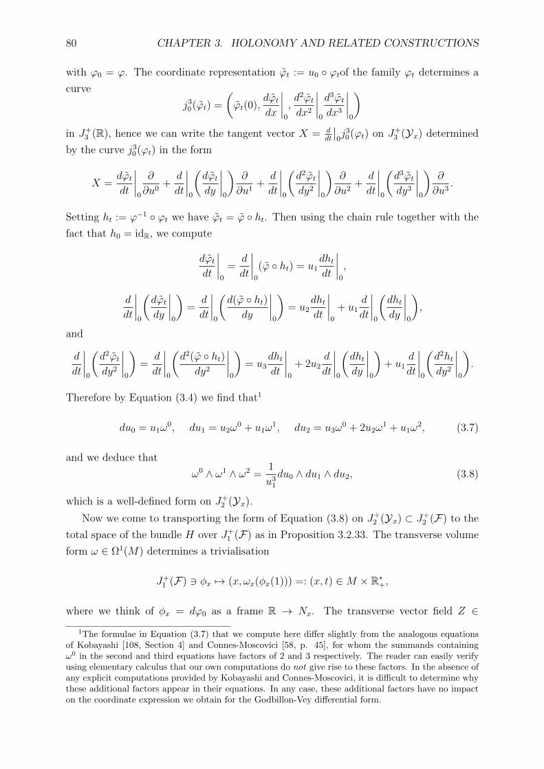
80 CHAPTER 3. HOLONOMY AND RELATED CONSTRUCTIONS
with ϕ0 = ϕ. The coordinate representation ϕt := u0 ϕtof the family ϕt determines a
curve
j30(ϕt) =
(ϕt(0),
dϕtdx
∣∣∣∣0
,d2ϕtdx2
∣∣∣∣0
d3ϕtdx3
∣∣∣∣0
)in J+
3 (R), hence we can write the tangent vector X = ddt
∣∣0j3
0(ϕt) on J+3 (Yx) determined
by the curve j30(ϕt) in the form
X =dϕtdt
∣∣∣∣0
∂
∂u0+d
dt
∣∣∣∣0
(dϕtdy
∣∣∣∣0
)∂
∂u1+d
dt
∣∣∣∣0
(d2ϕtdy2
∣∣∣∣0
)∂
∂u2+d
dt
∣∣∣∣0
(d3ϕtdy3
∣∣∣∣0
)∂
∂u3.
Setting ht := ϕ−1 ϕt we have ϕt = ϕ ht. Then using the chain rule together with the
fact that h0 = idR, we compute
dϕtdt
∣∣∣∣0
=d
dt
∣∣∣∣0
(ϕ ht) = u1dhtdt
∣∣∣∣0
,
d
dt
∣∣∣∣0
(dϕtdy
∣∣∣∣0
)=
d
dt
∣∣∣∣0
(d(ϕ ht)
dy
∣∣∣∣0
)= u2
dhtdt
∣∣∣∣0
+ u1d
dt
∣∣∣∣0
(dhtdy
∣∣∣∣0
),
and
d
dt
∣∣∣∣0
(d2ϕtdy2
∣∣∣∣0
)=
d
dt
∣∣∣∣0
(d2(ϕ ht)
dy2
∣∣∣∣0
)= u3
dhtdt
∣∣∣∣0
+ 2u2d
dt
∣∣∣∣0
(dhtdy
∣∣∣∣0
)+ u1
d
dt
∣∣∣∣0
(d2htdy2
∣∣∣∣0
).
Therefore by Equation (3.4) we find that1
du0 = u1ω0, du1 = u2ω
0 + u1ω1, du2 = u3ω
0 + 2u2ω1 + u1ω
2, (3.7)
and we deduce that
ω0 ∧ ω1 ∧ ω2 =1
u31
du0 ∧ du1 ∧ du2, (3.8)
which is a well-defined form on J+2 (Yx).
Now we come to transporting the form of Equation (3.8) on J+2 (Yx) ⊂ J+
2 (F) to the
total space of the bundle H over J+1 (F) as in Proposition 3.2.33. The transverse volume
form ω ∈ Ω1(M) determines a trivialisation
J+1 (F) 3 φx 7→ (x, ωx(φx(1))) =: (x, t) ∈M × R∗+,
where we think of φx = dϕ0 as a frame R → Nx. The transverse vector field Z ∈
1The formulae in Equation (3.7) that we compute here differ slightly from the analogous equationsof Kobayashi [108, Section 4] and Connes-Moscovici [58, p. 45], for whom the summands containingω0 in the second and third equations have factors of 2 and 3 respectively. The reader can easily verifyusing elementary calculus that our own computations do not give rise to these factors. In the absence ofany explicit computations provided by Kobayashi and Connes-Moscovici, it is difficult to determine whythese additional factors appear in their equations. In any case, these additional factors have no impacton the coordinate expression we obtain for the Godbillon-Vey differential form.

3.3. ALGEBRAS ASSOCIATED TO THE HOLONOMY GROUPOID 81
Γ∞(M ;N) corresponding to ω determines a trivialisation
N 3 hZx 7→ (x, h) ∈M × R, x ∈M.
of N and therefore a corresponding trivialisation H ∼= J+1 (F) × R ∼= M × R∗+×R of
H ∼= π∗1N . Unlike the coordinates ui used for the transversal Yx in the first part of the
proof, the trivialisation H ∼= M × R∗+×R is global, and we must show that on Yx, we
have equalities du0 = ω, u1 = t and u2 = h.
Now du0(Z) ≡ 1 by definition of the coordinate u0 on Yx so du0 = ω. For u1 we see
that
u1 =d(u0 ϕ)
dy= du0 dϕ(1) = ωx(dϕ(1)) = t
by definition of the variable t. Finally, in the trivial principal G+2 (1)-bundle J+
2 (R) =
R×G+2 (1) that is the image of J+
2 (Yx) under the coordinates (u0, u1, u2), the u2 variable
identifies with the tangent variable for R in the manner of Proposition 3.2.33. Viewed as
coordinates on J+2 (Yx) and T Yx respectively, we then have u2 = h and therefore
gv = − 1
u31
du0 ∧ du1 ∧ du2 = − 1
t3ω ∧ dt ∧ dh
as claimed.
Remark 3.2.35. The formalism discussed in this section regarding tautological differ-
ential forms on jet bundles is normally seen in the context of Gelfand-Fuks cohomology
of Lie algebras of vector fields, for which we refer the reader to the extensive literature
[75, 76, 78, 77, 28, 86, 24, 25, 90]. The (SO(q,R)-relative) Gelfand-Fuks complex of the
Lie algebra of formal vector fields on Rq naturally maps to the tautological differential
forms on the bundles J+k (F)/ SO(q,R) of any foliated manifold (M,F). Somewhat mirac-
ulously, at the cohomological level the classes obtained in this way are the same as those
obtained via the Chern-Weil method adopted here. In fact, the relative Gelfand-Fuks
cohomology is (up to a minor adjustment involving the Euler class of the normal bundle
for q even) the same as the cohomology of the truncated Weil algebra WOq [28, Theorem
2].
3.3 Algebras associated to the holonomy groupoid
For the entirety of this section let (M,F) denote a foliated manifold with holonomy
groupoid G. In this section we will introduce convolution algebras associated to G with
which we can use KK and cyclic theories.

82 CHAPTER 3. HOLONOMY AND RELATED CONSTRUCTIONS
3.3.1 The smooth convolution algebra
If G is a locally compact Hausdorff group, with Haar measure µ, one considers the space
Cc(G) of continuous, compactly supported, complex-valued functions on G, equipped
with the convolution product defined by
f1 ∗ f2(g) :=
∫G
f1(h)f2(h−1g)dµ(h)
and with the adjoint
f ∗(g) := f(g−1)
defined for all f, f1, f2 ∈ Cc(G). It can be shown [67, 13.9] that with these operations
Cc(G) is a ∗-algebra, and one considers the reduced group C∗-algebra associated to G.
The reduced C∗-algebra C∗r (G) of G is obtained by completing Cc(G) in its image under
the regular representation π : Cc(G) → L2(G, µ) in the Hilbert space L2(G, µ) of µ-
square-integrable functions G→ C given by
π(f)ξ(g) :=
∫G
f(h)ξ(h−1g)dµ(h)
for all f ∈ Cc(G) and ξ ∈ L2(G, µ). The representation theory of C∗r (G) is closely related
to the representation theory of G itself.
It was Renault [141] who first constructed the analogous algebras associated to lo-
cally compact topological groupoids. The formulae look superficially the same, with the
Haar measure µ replaced by a continuously varying system of measures on the fibres Gx,x ∈ G(0), known as a Haar system (see Definition B.6.1). Locally compact groupoids
are general enough objects that such Haar systems do not exist in general, in contrast
with locally compact groups which always admit a (left) Haar measure. Thankfully, the
holonomy groupoids associated to foliated manifolds are, despite their non-Hausdorffness,
nice enough that they admit Haar systems and therefore admit associated C∗-algebras.
In fact the smooth structure of holonomy groupoids allows us to define C∗-algebras in
an entirely intrinsic manner using density bundles, as recognised by Connes [53], whose
exposition we follow in this section.
Definition 3.3.1. The leafwise half-density bundle over M is the trivialisable
bundle |T F | 12 over M whose fibre |TxF |12 over x ∈ M is the space of all maps ρ :
Λdim(F)TxF → C such that ρ(λv) = |λ| 12ρ(v) for all v ∈ Λdim(F)TxF and λ ∈ R. The
leafwise half-density bundle over G is the trivialisable bundle
Ω12 := r∗|T F |
12 ⊗ s∗|T F |
12
over G.

3.3. ALGEBRAS ASSOCIATED TO THE HOLONOMY GROUPOID 83
One would like to define an algebra in a manner analogous to locally compact groups,
in which case one considers the space of compactly supported continuous functions. In
attempting the same construction for G we run into a problem that is now very well-
explored in the literature [53, 62, 151, 134]: G need not be Hausdorff and, as such, need
not admit any interesting compactly supported continuous (let alone smooth) functions at
all. In [62], Crainic and Moerdijk give a sheaf-theoretic approach to defining C∞c functions
on non-Hausdorff manifolds, which has certain advantages (for instance, a Mayer-Vietoris
sequence). We will not need the advantages provided by this sophisticated approach, and
adopt instead Connes’ older and more well-known solution [53, Section 6].
Definition 3.3.2. Denote by C∞c (G; Ω12 ) the space of finite sums of sections f of Ω
12 over
G which are zero outside of a Hausdorff open subset U of G, and are smooth with compact
support inside U .
When G is Hausdorff, C∞c (G; Ω12 ) of course coincides with the compactly supported
smooth sections of Ω12 over G. For G non-Hausdorff, elements of C∞c (G; Ω
12 ) need not be
globally continuous - the reason essentially being that locally defined continuous functions
on a non-Hausdorff space need not extend by zero to globally continuous functions. This
phenomenon is best illustrated using a simple example.
Example 3.3.3. Consider the line X with two origins:
X := (R \0) ∪ x, y,
equipped with the topology whose base is composed of charts of the form:
1. any open ball in R \0,
2. any set of the form (−a, 0) ∪ x ∪ (0, a), a > 0, and
3. any set of the form (−a, 0) ∪ y ∪ (0, a), a > 0.
Then the basis sets form an atlas for X so that X is a smooth manifold, but X is not
Hausdorff, as the points x and y cannot be separated by disjoint open sets.
Fix a > 0 and consider now any smooth, compactly supported bump function ϕ
defined on Ua := (−a, 0)∪x∪(0, a), for which ϕ(x) = 1. Extend ϕ by zero to a function
ϕ on X. Then ϕ is not continuous. Indeed, the sequence cn := 1nn∈N contained in the
chart Ua converges in X to both x and y. Since ϕ(x) = 1 while ϕ(y) = 0, ϕ cannot be
continuous.
Let us now come back to functions on G. The adjoint of f ∈ C∞c (G; Ω12 ) is relatively
easy to define:
f ∗(u) := f(u−1),

84 CHAPTER 3. HOLONOMY AND RELATED CONSTRUCTIONS
where λ denotes complex conjugation of the complex half-density λ. Let us now fix
f, g ∈ C∞c (G; Ω12 ). For u ∈ G and v ∈ Gr(u), we see that
f(v)g(v−1u) ∈ |Tr(v)F |12 ⊗ |Ts(v)F | ⊗ |Ts(u)F |
12 = s∗|T F |v ⊗ Ω
12u ,
using the symmetry of the tensor product of vector spaces. Since s : Gr(u) → Lr(u) is
a local diffeomorphism, v 7→ f(v)g(v−1u) defines an Ω12u -valued density on the manifold
Gr(u) and may be integrated thereover to give, by the compact support of f and g, a
well-defined element f ∗ g(u) ∈ Ω12u . Somewhat miraculously, the section f ∗ g of Ω
12
obtained in this way is again an element of C∞c (G; Ω12 ).
Proposition 3.3.4. Let f, g ∈ C∞c (G; Ω12 ). Then the functions f ∗ g and f ∗ defined on
G respectively for u ∈ G by
f ∗ g(u) :=
∫v∈Gr(u)
f(v)g(v−1u) f ∗(u) := f(u−1)
are elements of C∞c (G; Ω12 ).
Proof. In showing that f ∗ g ∈ C∞c (G; Ω12 ), we may assume without loss of generality
that f (resp. g) is smooth with compact support in some chart U1 (resp. U2), and zero
outside of U1 (resp. U2). If
U1U2 := uv : (u, v) ∈ U1 ×s,r U2
is empty, then for each u ∈ G and v ∈ Gr(u) one has f(v)g(v−1u) = 0. Thus in this case
f ∗ g vanishes identically on G and is equal to the trivial element of C∞c (G; Ω12 ).
Let us assume instead that U1U2 6= ∅, and write Ui = Bri,τ ×Bs
i,τ ×Vi for each i = 1, 2,
where Bri,τ and Bs
i,τ are open balls in Rdim(F) and Vi an open ball in Rq, for which Bri,τ×Vi
and Bsi,τ × Vi are foliated coordinate charts for (M,F). Since U1U2 6= ∅ we may assume
without loss of generality that Bs1,τ = Br
2,τ and that V1 = h(V2), where h : V2 → V1 is a
holonomy diffeomorphism. In the coordinates (x, y, z) ∈ Br1,τ ×Bs
2,τ × V2 we then have
f ∗ g(x, y, z) =
∫y′∈Bs1,τ
f(x, y′, h(z))g(y′, y, z)dy′.
By the smoothness and compact support of f and g on U1 and U2 respectively we then
see that f ∗ g is a smooth function with compact support on the chart U1U2, so extends
by zero on G to give an element of C∞c (G; Ω12 ).
To see that the adjoint f ∗ of f is an element of C∞c (G; Ω12 ) we similarly assume without
loss of generality that f is smooth with compact support in some chart U = Brτ ×Bs
τ ×Vof G. Since the pointwise conjugation · is a smooth operation on the vector bundle Ω
12

3.3. ALGEBRAS ASSOCIATED TO THE HOLONOMY GROUPOID 85
and since inversion ι on G is a diffeomorphism, we see that f ∗ = · f ι is smooth with
compact support in the chart U−1 = Bsτ×Br
τ×V so defines an element of C∞c (G; Ω12 ).
The following is now easily checked by direct calculation.
Proposition 3.3.5. The space C∞c (G; Ω12 ), equipped with the convolution product and
adjoint of Proposition 3.3.4, is a ∗-algebra.
3.3.2 The C∗-algebra
In this subsection we continue to follow the fairly direct and foliation-specific treatment
given by Connes [53]. For a more general treatement we refer to [110, 107, 134], and to
Appendix B.
The C∗-algebra of a foliation is constructed from the ∗-algebra C∞c (G; Ω12 ) associ-
ated to its holonomy groupoid G, together with a canonical family of representations
parametrised by the unit space M of G. Specifically, for each x ∈ M one defines the
Hilbert space L2(Gx; r∗|T F |12 ) of sections of r∗|T F | 12 over the Hausdorff submanifold
Gx of G which are square-integrable in the sense that∫u∈Gx|ξ(u)|2 <∞.
Here |ξ(u)|2 = ξ(u)ξ(u) ∈ |Tr(u)F |12 ⊗ |Tr(u)F |
12 = |Tr(u)F | for each u ∈ G. Thus, since
r : Gx → Lx is a local diffeomorphism onto the leaf through x, the map u 7→ |ξ(u)|2 is a
density on Gx and its integral makes sense. We obtain a representation πx : C∞c (G; Ω12 )→
L(L2(Gx; r∗|T F |12 )) as follows.
Proposition 3.3.6. For x ∈M , f ∈ C∞c (G; Ω12 ) and ξ ∈ L2(Gx; r∗|T F |
12 ), the formula
πx(f)ξ(u) :=
∫v∈Gr(u)
f(v)ξ(v−1u), u ∈ Gx
defines a bounded operator πx(f) on L2(Gx; r∗|T F |12 ) and determines a ∗-homomorphism
πx : C∞c (G; Ω12 )→ L(L2(Gx; r∗|T F |
12 )).
Proof. Fix f ∈ C∞c (G; Ω12 ) and ξ ∈ L2(Gx; r∗|T F |
12 ). First observe that for any u ∈ Gx
and for any v ∈ Gr(u), we have
f(v)ξ(v−1u) ∈ |Tr(v)F |12 ⊗ |Ts(v)F |
12 ⊗ |Ts(v)F |
12 = |Tr(u)F |
12 ⊗ |Ts(v)F |.
Therefore v 7→ f(v)ξ(v−1u) is a |Tr(u)F |12 -valued density on Gr(u) so the integral makes
sense, and yields a finite value for each u ∈ G since the restriction of f to the Hausdorff
manifold Gr(u) is smooth with compact support.

86 CHAPTER 3. HOLONOMY AND RELATED CONSTRUCTIONS
To show that πx(f) is a bounded operator let us assume without loss of generality that
f is zero outside some chart U = Brτ×Bs
τ×V of G, with Us = Bsτ×V and Ur = Br
τ×h(V )
precompact foliated charts for M and h : V → h(V ) a holonomy diffeomorphism, and is
smooth with compact support inside of U . Then πx(f) can be viewed as the integral oper-
ator on L2(Gx; Ω12 ) with integral kernel k(w1, w2) := f(w1w
−12 ) ∈ |Tr(w1)F |
12⊗|Tr(w2)F |
12 ,
w1, w2 ∈ Gx. That is,
πx(f)ξ(u) =
∫v∈Gr(u)
f(v)ξ(v−1u) =
∫w=v−1u∈Gx
f(uw−1)ξ(w) =
∫w∈Gx
k(u,w)ξ(w)
for all u ∈ Gx.Now by the proof of Lemma 3.1.14 r : Gx → Lx is a covering map, whose deck
transformation group is the countable discrete group Gxx acting on Gx via Gx×Gxx 3(w, u) 7→ wu ∈ Gx. For any u ∈ Gxx we have
k(w1u,w2u) = f(w1uu−1w−1
2 ) = f(w1w−12 ) = k(w1, w2)
for all (w1, w2) ∈ Gx×Gx, so k is invariant under the action of Gxx and therefore descends
to a smooth section k of the bundle proj∗1 |T F |12 ⊗ proj∗2 |T F |
12 over Lx ×Lx defined by
k(r(w1), r(w2)) := k(w1, w2) = f(w1w−12 ) ∈ |Tr(w1)F |
12 ⊗ |Tr(w2)F |
12
for any w1, w2 ∈ Gx. Now since f is zero outside U and has compact support K ⊂ U
therein, we see that k is zero outside the compact set (r(K) ∩ Lx) × (s(K) ∩ Lx) in
Lx×Lx. Since r|Gx is a covering map, r(K)∩Lx (resp. s(K)∩L) is covered by a pairwise
disjoint family Kuu∈Gxx (resp. K ′uu∈Gxx) of compact subsets of Gx, and we can write
k =∑
u∈Gxxku where each ku is smooth with compact support in Ku×K ′u. In particular,
each ku is a Hilbert-Schmidt operator with operator norm
‖ku‖2 =
∫(w1,w2)∈Gx×Gx
|ku(w1, w2)|2 =
∫(r(w1),r(w2))∈Lx×Lx
|k(r(w1), r(w2))|2 = ‖k‖2HS
independent of u.
That the ku have mutually disjoint supports implies that k∗ukv = 0 for all u 6= v in Gxx.We denote by pu the projection onto the closure of the range of k∗u, so that kuξ = kupuξ
for all ξ ∈ L2(Gx; r∗|T F |12 ). Denoting ‖ · ‖
L2(Gx;r∗|T F |12 )
by ‖ · ‖ for simplicity, we can
now estimate
‖πx(f)ξ‖2 =
∥∥∥∥ ∑u∈Gxx
kuξ
∥∥∥∥2
=∑u,v∈Gxx
(kuξ|kvξ) =∑u,v∈Gxx
(kupuξ|kvpvξ) =∑u,v∈Gxx
(puξ|k∗ukvpvξ)
=∑u∈Gxx
(puξ|k∗ukupuξ) ≤ supu∈Gxx‖ku‖2
∑u∈Gxx
‖puξ‖2 ≤ ‖k‖2HS‖ξ‖2.

3.3. ALGEBRAS ASSOCIATED TO THE HOLONOMY GROUPOID 87
Thus πx(f) is a bounded operator on L2(Gx; r∗|T F |12 ). A routine calculation using the
convolution formulae shows that the map πx : C∞c (G; Ω12 ) → L(L2(Gx; r∗|T F |
12 )) is a
∗-homomorphism.
Since the πx are all ∗-homomorphisms, all the norms induced on C∞c (G; Ω12 ) by the πx
are C∗-norms. Moreover if K is a compact subset of a Hausdorff open set in G, then K
intersects only compactly many of the Gx, so for any f ∈ C∞c (G; Ω12 ) the supremum over
x of the ‖πx(f)‖ is finite. We may therefore complete C∞c (G; Ω12 ) in the corresponding
supremum norm to obtain the C∗-algebra of (M,F).
Definition 3.3.7. The (reduced) C∗-completion C∗r (G) of C∞c (G; Ω12 ) in the norm
‖f‖C∗r (G) := supx∈M‖πx(f)‖
L(L2(Gx;r∗|T F |12 ))
is called the reduced C∗-algebra of G or the C∗-algebra of (M,F).
Remark 3.3.8. Since G is second-countable, C∗r (G) is separable [141, Page 59].

88 CHAPTER 3. HOLONOMY AND RELATED CONSTRUCTIONS
Chapter 4
Characteristic classes on the
holonomy groupoid
The characteristic classes given in Theorem 2.4.21 for a foliated manifold (M,F) arise
from geometries associated to the normal bundle N . Since the normal bundle of any
foliated manifold carries an action of the holonomy groupoid G by Proposition 3.2.1,
one might expect it to be possible to encode both the geometry of the normal bundle
and the dynamics of the holonomy groupoid simultaneously so as to produce topological
information for G. One would naturally require such information to coincide with the
usual characteristic classes on M when considering the “static” unit space M ⊂ G.
In order to study such phenomena, it has become standard practice in the literature
[55, 60, 82, 57, 83, 64, 130, 58] to “etalify” the holonomy groupoid as follows. One takes
any q-dimensional submanifold T ⊂M which intersects each leaf of F at least once, and
which is everywhere transverse to F in the sense that Tx T ⊕TxF = TxM for all x ∈ T .
Such a submanifold is called a complete transversal for (M,F). Having chosen such a
complete transversal T we consider the subgroupoid
GTT := u ∈ G : r(u), s(u) ∈ T
of G. The subgroupoid GTT inherits from G a differential topology for which it is a (gener-
ally non-Hausdorff) etale Lie groupoid [63, Lemma 2] - that is, a Lie groupoid whose range
(and therefore source) are local diffeomorphisms. For any choice of complete transversal
T , the groupoids G and GTT are Morita equivalent [63, Lemma 2]. Consequently they are
(co)homologically identical [63, 64], and have Morita equivalent C∗-algebras [134] so are
the the same as far as K-theory is concerned also.
The purpose of this chapter is to give, for the first time, analogous characteristic
maps to those defined in [57, 64] in the context of the full holonomy groupoid of a
foliated manifold. Our characteristic map will be constructed in a Chern-Weil fashion
from Bott connections for N just as in Theorem 2.4.21. We recall the required technology
89
90CHAPTER 4. CHARACTERISTIC CLASSES ON THE HOLONOMY GROUPOID
of [114] in the first section of this chapter for the reader’s convenience. The second section
onwards consists of original work except where stated otherwise. In particular, we prove
in Theorem 4.2.2 a generalisation of Bott’s vanishing theorem (see Theorem 2.4.18), and
deduce a characteristic map from the cohomology of WOq to the de Rham cohomology
of the full holonomy groupoid of the frame bundle. These results should be thought of as
the non-etale analogues of [64, Theorem 2 (iv)] and [57, Lemma 17] respectively. We also
derive in the third section a Godbillon-Vey cyclic cocycle (see Proposition 4.3.6), which
should be thought of as an analogue of the Connes-Moscovici formula [58, Proposition
19], and will be used for comparison with the Godbillon-Vey index formula obtained in
the next chapter.
Let us stress that the approach taken in this thesis has the advantage of being in-
trinsically geometric, giving representatives of cohomological data that are expressed in
terms of global geometric data for (M,F). For instance, the Godbillon-Vey cyclic cocycle
obtained in this thesis has a completely novel interpretation in terms of line integrals of
the Bott curvature over paths in F representing elements of G (see Proposition 4.3.1).
This is to be contrasted with the approaches taken in the etale context, in which the ge-
ometry of M has necessarily been lost in “chopping up” G into GTT . In the etale context,
explicit formulae have so far tended to be obtained by tracking the displacement of local
geometric data (trivial connections in local transversals) [64, 58, Section 5.1, p. 47] under
the action of GTT , which will in general not be easily relatable to the global geometry of
M .
4.1 Chern-Weil homomorphism for Lie groupoids
The Chern-Weil map we construct is adapted for foliations from the paper [114], whose
historical antecedents are to be found in the papers [70, 29].
Just as the classical Chern-Weil theory can be simplified and systematised by using
principal G-bundles, Chern-Weil theory at the level of Lie groupoids is most easily studied
using principal bundles over groupoids. For the entirety of this section we let G be a (not
necessarily Hausdorff) Lie groupoid, with unit space G(0), and let G be a Lie group.
Definition 4.1.1. A principal G-bundle over G consists of a principal G-bundle
π : P(0) → G(0) over G(0) together with an action σ : P := G ×s,π P(0) → P(0) that
commutes with the right action of G on P(0). We will often refer to P as a principal
G-groupoid over G.
Let us for the rest of this section fix a principal G-bundle π : P(0) → G(0) over G. We
have already seen that P itself is a Lie groupoid with unit space P(0) (see Proposition
3.2.2), and we can therefore consider the spaces P(k) of composable k-tuples of elements
of P . In order to make notation less cumbersome, for (u1, . . . , uk) ∈ G(k) and p ∈ P (0)s(uk)
4.1. CHERN-WEIL HOMOMORPHISM FOR LIE GROUPOIDS 91
we will denote the composable k-tuple
((u1, (u2 · · ·uk) · p), (u2, (u3 · · ·uk) · p), . . . , (uk, p)
)∈ P(k)
by simply
(u1, . . . , uk) · p.
The next result tells us that the P(k) fibre over the G(k) as principal G-bundles, and is a
straightforward consequence of the fact that P(0) → G(0) is a principal G-bundle, together
with the fact that the action of G commutes with that of G.
Lemma 4.1.2. Let π : P(0) → G(0) be a principal G-bundle over G. Then for each k ∈ Nand (u1, . . . , uk) · p ∈ P(k), the formula
π(k)((u1, . . . , uk) · p) := (u1, . . . , uk)
defines a principal G-bundle π(k) : P(k) → G(k).
Remark 4.1.3. Note that the definition and properties of the exterior derivative d on
a manifold Y depend only on the local structure of the manifold. Consequently, the
differential forms (Ω∗(Y ), d) on Y are a differential graded algebra whether Y is Hausdorff
or not. We will use this fact freely and without further comment in what follows.
We saw in Construction 3.2.11 that for a transversely orientable foliated manifold
(M,F), the differential forms Ω∗(Fr+(N)) form a GL+(q,R)-differential graded algebra.
We point the reader to Example D.2.6 in the Appendix to see that this phenomenon is
more general. Specifically, if G is a Lie group, then the differential forms Ω∗(P ) on any
principal G-bundle P form a G-differential graded algebra, and if K is any Lie subgroup
of G then the K-basic elements of Ω∗(P ) can be identified with Ω∗(P/K). We then have
the following immediate consequence of Lemma 4.1.2.
Corollary 4.1.4. For all k ∈ N, the differential forms Ω∗(P(k)) on P(k) form a G-
differential graded algebra. If K ⊂ G is a Lie subgroup, then the K-basic elements of
Ω∗(P(k)) identify with the differential forms Ω∗(P(k) /K) on the quotient of P(k) by the
right action of K.
Let us now recall the definition of the de Rham cohomology of P as a Lie groupoid
together with its relative versions.
Observe that there exist face maps εki : P(k) → P(k−1) defined for all k > 1 and
0 ≤ i ≤ k by the formulae
εk0((u1, u2, . . . , uk) · p
):= (u2, . . . , uk) · p,
εkk((u1, . . . , uk) · p
):= (u1, . . . , uk−1) · (uk · p),

92CHAPTER 4. CHARACTERISTIC CLASSES ON THE HOLONOMY GROUPOID
and
εki((u1, . . . , uk) · p
):= (u1, . . . , uiui+1, . . . , uk) · p
for 1 ≤ i ≤ k − 1. For k = 1, we obtain the obvious maps ε10 := s : P → P(0) and
ε11 := r : P → P(0) = M .
Remark 4.1.5. The collection P(k)k≥0, taken together with the face maps εki : P(k) →P(k−1), is known in the literature as the nerve N P of P . The nerve N P is an example of
a (semi) simplicial manifold (the terminology used depends on the author). It is in the
general setting of simplicial manifolds that most of the technology in this chapter was
developed by Bott-Shulman-Stasheff [29] and Dupont [69, 70].
The next result is an immediate consequence of the fact that the action of G on P(0)
commutes with the right action of G on P(0).
Lemma 4.1.6. The face maps εki : P(k) → P(k−1) commute with the actions of G on P(k)
and P(k−1).
Since each P(k) is a manifold, the exterior derivative d : Ω∗(P(k)) → Ω∗+1(P(k)) is
defined for all k ≥ 0 and satisfies the usual property d2 = 0. The exterior derivative will
form the vertical differential of the double complex from which we will construct the de
Rham cohomology of P . To obtain the horizontal differential, notice that the face maps
εki : P(k) → P(k−1) allow us to define a natural map ∂ : Ω∗(P(k−1)) → Ω∗(P(k)) via an
alternating sum of pullbacks
∂ω :=k∑i=0
(−1)i(εki )∗ω.
A routine calculation shows that ∂2 = 0. By Lemma 4.1.6 the coboundary mapping
∂ : Ω∗(P(k−1))→ Ω∗(P(k)) preserves K-basic elements for any Lie subgroup K of G, and
we therefore obtain the double complex
......
...
Ω1(P(0) /K) Ω1(P(1) /K) Ω1(P(2) /K) · · ·
Ω0(P(0) /K) Ω0(P(1) /K) Ω0(P(2) /K) · · ·
d
d
d d
d d
∂ ∂ ∂
∂ ∂ ∂
4.1. CHERN-WEIL HOMOMORPHISM FOR LIE GROUPOIDS 93
Definition 4.1.7. Let K be a Lie subgroup of G. The double complex (Ω∗(P(∗) /K), d, ∂)
is called the K-basic de Rham complex of the principal G-groupoid P. The associated
total complex is given by
Tot∗Ω(P /K) =⊕
n+m=∗
Ωn(P(m) /K), δ|Ωn(P(m) /K) := (−1)md+ ∂.
The cohomology of (Tot∗Ω(P /K), δ) is denoted by H∗dR(P /K) and is called the K-basic
de Rham cohomology of the principal G-groupoid P.
Remark 4.1.8. The de Rham complex of Definition 4.1.7 is frequently referred to in
the literature as the Bott-Shulman-Stasheff complex associated to the simplicial manifold
N(P /K), named after its originators [29].
In the same way that the exterior product of differential forms induces a multiplication
in de Rham cohomology groups of any manifold, the exterior product of differential forms
also induces a multiplication in the de Rham cohomology of G.
Definition 4.1.9. Let K be a Lie subgroup of G. Given ω1 ∈ Ωk(P(m) /K) and ω2 ∈Ωl(P(n) /K) we define the cup product ω1 ∨ ω2 ∈ Ωk+l(P(m+n) /K) of ω1 and ω2 by
(ω1 ∨ ω2)(u1,...,um+n) := (−1)kn(p∗1ω1)(u1,...,um+n) ∧ (p∗2ω2)(u1,...,um+n),
where p1 : P(m+n) /K → P(m) /K is given by
p1(u1, . . . , um+n) =
(u1, . . . , um) if m ≥ 1
r(u1) if m = 0, n ≥ 1
id if m = n = 0
and p2 : P(m+n) /K → P(n) /K is given by
p2(u1, . . . , um+n) =
(um+1, . . . , um+n) if n ≥ 1
s(um) if n = 0,m ≥ 1
id if m = n = 0
Proposition 4.1.10. The cup product descends to give a well-defined multiplication on
H∗dR(P /K), gifting H∗dR(P /K) the structure of a graded ring.
Proof. The cup product respects the bi-grading of Ω∗(P(∗) /K) by definition. Well-
definedness on H∗dR(P /K) follows from the Liebniz rule for the exterior derivative, and
from noting that we may rewrite p1 : P(m+n) /K → P(m) /K as
p1 = εm+1m+1 · · · εm+i
m+i · · · εm+nm+n

94CHAPTER 4. CHARACTERISTIC CLASSES ON THE HOLONOMY GROUPOID
and p2 : P(m+n) /K → P(n) /K as
p2 = εn+10 · · · εn+i
0 · · · εn+m0 ,
where the εki : P(k) → P(k−1) are the face maps.
For our characteristic map we will also need a particular differential graded algebra
which encodes the face maps of the P(k) into those of the standard simplices. For k ∈ N,
let ∆k denote the standard k-simplex
∆k :=
(t0, t1, . . . , tk) ∈ [0, 1]k+1 :
k∑i=0
ti = 1
. (4.1)
We have face maps εki : ∆k−1 → ∆k defined for all k > 1 and 1 ≤ i ≤ k by the formulae
εki (t0, . . . , tk−1) := (t0, . . . , ti−1, 0, ti, . . . , tk−1).
and for i = 0 by simply
εk0(t0, . . . , tk−1) := (0, t0, . . . , tk−1).
Definition 4.1.11. For l ∈ N, a simplicial l-form on P is a sequence ω = ω(k)k∈Nof differential l-forms ω(k) ∈ Ωl(∆k × P(k)) such that
(εki × id)∗ω(k) = (id×εki )∗ω(k−1) ∈ Ωl(∆(k−1) × P(k))
for all i = 0, . . . , k and for all k ∈ N. We denote the space of all simplicial l-forms on Pby Ωl
∆(P).
Remark 4.1.12. One defines the fat realisation ‖N P ‖ of N P to be the space
‖N P ‖ :=⊔k≥0
(∆k × P(k)
)/ ∼,
where we identify (t, εki (v)) ∈ ∆k−1 × P(k−1) with (εki (t), v) ∈ ∆k × P(k) for all k > 0,
t ∈ ∆k−1 and v ∈ P(k). The fat realisation is a geometric realisation of the classifying
space B P of the groupoid P [145], and is not generally a manifold even though each of
its “layers” ∆k × P(k) is. Simplicial differential forms were defined by Dupont [70] so
as to descend to “forms on B P”. We will see shortly that together with the usual de
Rham differential, simplicial differential forms define a differential graded algebra whose
cohomology can be taken as the definition of the cohomology of the classifying space.
Importantly, simplicial differential forms on P determine a differential graded algebra

4.1. CHERN-WEIL HOMOMORPHISM FOR LIE GROUPOIDS 95
which will be instrumental in the construction of our characteristic map.
Proposition 4.1.13. The wedge product and exterior derivative of differential forms on
the manifolds ∆k ×P(k) together with the action of G on the P(k) make the space Ω∗∆(P)
of all simplicial differential forms on P into a G-differential graded algebra. If K is any
Lie subgroup of G, then the subcomplex (Ω∗∆(P)K−basic, d) of (Ω∗∆(P), d) coincides with
the complex (Ω∗∆(P /K), d) of simplicial differential forms on the groupoid P /K.
Proof. To show that Ω∗∆(P) is a differential graded algebra we just need to show that the
exterior derivative and wedge product of simplicial differential forms is again a simplicial
differential form. Let ω = ω(k)k∈N be a simplicial differential form, and consider the
sequence dω = dω(k)k∈N. For each k > 0 and each i = 0, . . . , k we use the commutativity
of the exterior derivative with pullbacks to calculate
(εki × id)∗dω(k) = d((εki × id)∗ω(k)
)= d((id×εki )∗ω(k−1)
)= (id×εki )∗dω(k−1)
so that dω is a simplicial differential form. A similar calculation using the fact that
pullbacks distribute over the wedge product shows that if ω = ω(k)k∈N and η = η(k)k∈Nare simplicial differential forms then the sequence ω ∧ η := ω(k) ∧ η(k)k∈N defines a
simplicial differential form. Taking the space Ω∗∆(P) to be graded by degree of simplicial
differential forms then shows that Ω∗∆(P) is a differential graded algebra.
Now since each P(k) carries a right action of G, so too does each ∆k ×P(k) by taking
G to act as the identity on the first factor; we write Ak : ∆k × P(k)×G→ ∆k × P(k) for
these actions, and define, for a simplicial differential form ω = ω(k)k∈N,
g · ω := (Akg−1)∗ω(k)k∈N (4.2)
for all g ∈ G. For each k > 0 and for each 0 ≤ i ≤ k, since G acts trivially on the
standard simplex factor we have Akg−1 (εki × id) = (εki × id) Akg−1 for all g ∈ G, while by
Lemma 4.1.6 we moreover have εki Akg−1 = Ak−1g−1 εki for all g ∈ G. Hence
(εki × id)∗(Akg−1)∗ω(k) = (Akg−1)∗(εki × id)∗ω(k)
= (Akg−1)∗(id×εki )∗ω(k−1)
= (id×εki )∗(Ak−1g−1 )∗ω(k−1)
so that the formula (4.2) defines an action of G on Ω∆(P).
For X ∈ g and k ∈ N the fundamental vector field V X,k on the G-space ∆k × P(k) is
given by the formula
V X,k(t0,...,tk;u1,...,uk) :=
d
dt
∣∣∣∣t=0
Aexp(tX)(t0, . . . , tk;u1, . . . , uk).
96CHAPTER 4. CHARACTERISTIC CLASSES ON THE HOLONOMY GROUPOID
We let ιV X,k denote the interior product of forms on ∆k×P(k) with the vector field V X,k.
Since the action of G preserves simplicial differential forms, the formula
iXω := ιV X,kω(k)k∈N
defines a degree -1 derivation of Ω∆(P) for all X ∈ g. Now for X ∈ g, since V X,k is the
fundamental vector field on ∆k × P(k) it transforms under dAk by the formula
(dAkg)(t0,...,tk;(u1,...,uk)·p)(V X,k
(t0,...,tk;(u1,...,uk)·p))
= VAdg−1 (X),k
Akg(t0,...,tk;(u1,...,uk)·p). (4.3)
Together with the usual properties of the exterior derivative and contraction with vector
fields, Equation (4.3) implies that (Ω∗∆(P), d, i) is a G-differential graded algebra. Now
if K is a Lie subgroup of G, the K-basic elements coincide with Ω∗∆(P /K) by the same
arguments as in Example D.2.6.
In order to relate simplicial differential forms back to the de Rham cohomology of P ,
we make use of the integration over the fibres map.
Proposition 4.1.14. Let K be a Lie subgroup of G. Then the map I : Ω∗∆(P /K) →Tot∗Ω(P /K) defined by
I(ω) :=∑l∈N
∫∆l
ω(l)
is a map of cochain complexes. Moreover the map determined by I on cohomology is
a homomorphism of rings, where the ring structure on H∗(Ω∗∆(P /K)) is induced by the
wedge product and where the ring structure on Tot∗Ω(P /K) is induced by the cup product.
Proof. Fix a K-basic simplicial differential form ω = ω(k)k∈N. By Proposition 4.1.13,
each ω(k) can be regarded as a form on the product manifold ∆k × (P(k) /K) over which
we can write
dω(k) = d1ω(k) + (−1)deg1 ω
(k)
d2ω(k),
where d1 is the exterior derivative in the ∆k variables, d2 is the exterior derivative in the
P(k) /K variables, and where deg1 ω(k) is the degree of the differential form ω(k) in the
∆k variables. Since d2 doesn’t interact with the ∆k variables we have∫∆k
d2ω(k) = d2
(∫∆k
ω(k)
).
On the other hand, Stokes’ theorem implies that∫∆k
d1ω(k) =
∫∂∆k
ω(k),

4.1. CHERN-WEIL HOMOMORPHISM FOR LIE GROUPOIDS 97
the right hand side of which we can compute using the face maps for the standard simplex:
∫∂∆k
ω(k) =k∑i=0
(−1)i∫
∆k−1
(εki × id)∗ω(k) =k∑i=0
(−1)i∫
∆k−1
(id×εki )∗ω(k−1)
=k∑i=0
(−1)i(εki )∗∫
∆(k−1)
ω(k−1) = ∂
(∫∆k−1
ω(k−1)
).
Therefore
I(dω) =I(d1ω + (−1)deg1 ωd2ω) =∑k∈N
∫∆k
(d1ω(k) + (−1)deg1 ω
(k)
d2ω)
=∑k∈N
(∂
∫∆k−1
ω(k−1) + (−1)deg1 ω(k)
d
∫∆k
ω(k)
)= (∂ + (−1)deg1 ωd)I(ω),
making I a map of cochain complexes as claimed.
The proof of the final claim is rather more involved, and we refer the reader to [70,
Theorem 2.14].
Remark 4.1.15. When G is Hausdorff, the map I : Ω∗∆(P /K)→ Tot∗Ω(P /K) descends
to an isomorphism on cohomology [70, Theorem 2.3]. Thus for Hausdorff G the double
complex Ω∗(G(∗)) computes the cohomology of the classifying space B G.
Before we give the characteristic map, we need to show that a connection form on P(0)
induces a connection on the differential graded algebra Ω∗∆(P). The universal property
of the Weil algebra W (g) (Theorem D.2.11) will then guarantee a homomorphism from
W (g) to Ω∗∆(P) which, composed with the cochain map I, will give us our characteristic
map.
Construction 4.1.16. For each 0 ≤ i ≤ k, define pki : P(k) → P(0) by
pk0((u1, . . . , uk) · p) := (u1 · · ·uk) · p,
pkk((u1, . . . , uk) · p) := p,
and
pki ((u1, . . . , uk) · p) := (ui+1 · · ·uk) · p.
for all 1 ≤ i ≤ k − 1. Since the range and source maps are G-equivariant, so too are the
maps pki . Given a connection form α ∈ Ω1(P(0); g), for each k ∈ N we define a differential
form α(k) ∈ Ω1(∆k × P(k); g) by the formula
α(k)(t0,...,tk;(u1,...,uk)·p) :=
k∑i=0
ti((pki )∗α)(u1,...,uk)·p. (4.4)

98CHAPTER 4. CHARACTERISTIC CLASSES ON THE HOLONOMY GROUPOID
We will show in the next lemma that the family α(k)k∈N, coming from a connection
form on P(0), is vertical and G-invariant, and consequently defines a connection on the
differential graded algebra Ω∗∆(P) (see Definition D.2.8).
Lemma 4.1.17. The sequence α := α(k)k∈N of 1-forms α(k) ∈ Ω1(∆k × P(k)) ⊗ g
determine a connection on the differential graded algebra Ω∗∆(P).
Proof. It is a routine verification that α is a simplicial 1-form on P . For instance, for
k ∈ N and for any (t0, . . . , tk−1; (u1, . . . , uk) · p) ∈ ∆k−1 × P(k) we calculate
((εk0 × id)∗α(k))(t0,...,tk−1;(u1,...,uk)·p) =α(k)(0,t0,...,tk−1;(u1,...,uk)·p)
=k−1∑j=0
tj(pkj+1)∗α(u1,...,uk)·p
=α(k)(t0,...,tk−1;(u2,...,uk)·p)
=((id×εk0)∗α(k))(t0,...,tk−1;(u1,...,uk)·p),
and similar calculations show that (εki ×id)∗α(k) = (id×εki )∗α(k) for i ≥ 1. Thus it remains
only to check the conditions of Definition D.2.8.
Since the pki : P(k) → P(0) are all equivariant with respect to the right action of
G, each (pki )∗α ∈ Ω1(∆k × P(k); g) is G-invariant by the corresponding property of α
as a connection form on P(0). Because the action of G on the space Ω∗(∆k × P(k))
distributes over addition of differential forms, the sum α(k) =∑ti((p
ki )∗α) is therefore
also G-invariant.
Finally, since the coordinates in the simplex sum to 1 and since iXα = 1 ⊗ X ∈Ω0(P(0))⊗ g, for any X ∈ g we have
iXα(k)(t0,...,tk;(u1,...,uk)·p) =
k∑i=0
tiiX(pki )∗α(u1,...,uk)·p =
k∑i=0
tiX = X
for all k ∈ N, and therefore iX α = 1⊗X ∈ Ω0∆(P)⊗ g.
Finally we can give the characteristic map as in [114].
Theorem 4.1.18. A choice of connection form α ∈ Ω1(P(0); g) determines, for any Lie
subgroup K of G, a homomorphism
φα : W (g, K)→ Ω∗∆(P /K)
of differential graded algebras, hence a cochain map
ψα = I φα : W (g, K)→ Tot∗Ω(P /K)

4.2. CHARACTERISTIC MAP FOR FOLIATED MANIFOLDS 99
of total complexes. The induced map on cohomology is a homomorphism of graded rings
and does not depend on the connection chosen.
Proof. The existence of φα follows from Lemma 4.1.17 together with Theorem D.2.11.
That ψα is a cochain map is true by Proposition 4.1.14, while the cohomological inde-
pendence of the choice of connection follows from Theorem D.2.11. That ψα descends to
a homomorphism H∗(W (g, K)) → H∗dR(P /K) of graded rings follows from Proposition
4.1.14 together with the fact that φα : W (g, K) → Ω∗∆(P /K) is a homomorphism of
differential graded algebras.
4.2 Characteristic map for foliated manifolds
Let us now consider a transversely orientable foliated manifold (M,F) of codimension
q. We have already seen in Example 3.2.7 that the positively oriented transverse frame
bundle Fr+(N) → M is a principal GL+(q,R)-bundle over the holonomy groupoid G of
(M,F). All results we present in this section are original.
Definition 4.2.1. We will denote by G1 = GnFr+(N) the principal GL+(q,R)-groupoid
over G corresponding to the foliated principal GL+(q,R)-bundle πFr+(N) : Fr+(N)→M .
By Theorem 4.1.18 and Corollary D.3.6, making a choice of connection form α ∈Ω1(Fr+(N); gl(q,R)) determines a cochain map ψα : WOq → Ω∗(G(∗)
1 / SO(q,R)), whose
induced map on cohomology does not depend on the connection α. Recall that within
WOq is the subalgebra I∗q (R) = R[c1, . . . , cq] generated by the invariant polynomials
ci(A) := Tr(Ai), A ∈ gl(q,R).
If we choose a Bott connection α[ ∈ Ω1(Fr+(N); gl(q,R)) for the definition of the
characteristic map ψα[ , we can prove the following generalisation of Theorem 2.4.18. This
theorem is original, and should be thought of as a non-etale analogue of [64, Theorem 2
(iv)].
Theorem 4.2.2 (Bott’s vanishing theorem for G1). Let α[ ∈ Ω1(Fr+(N); gl(q,R)) be
a connection form corresponding to a Bott connection ∇[ on N . If P ∈ I∗q (R) is an
invariant polynomial of degree deg(P ) > q (so that its degree in I∗q (R) is greater than 2q),
then ψα[(P ) = 0 ∈ Ω∗(G(∗)1 / SO(q,R)).
Proof. For each k ∈ N, let (R[)(k) = d(α[)(k) + (α[)(k) ∧ (α[)(k) denote the curvature of
the connection form (α[)(k) on ∆k × G(k)1 obtained as in Lemma 4.1.17. The cochain
ψα[(P ) in Ω∗(G(∗)1 / SO(q,R)) identifies in the same manner as in Example D.2.6 with the
SO(q,R)-basic cochain ∑k
∫∆k
P ((R[)(k)), (4.5)

100CHAPTER 4. CHARACTERISTIC CLASSES ON THE HOLONOMY GROUPOID
in Ω∗(G(∗)1 ). Thus it suffices to show that the cochain in Equation (4.5) is zero.
The form (R[)(k) is by construction of degree at most 1 in the ∆k variables due to
the d(α[), and therefore P ((R[)(k)) is of degree at most deg(P ) in the ∆k variables. Thus∫∆k P ((R[)(k)) vanishes when deg(P ) < k, implying that ψα(P ) vanishes in Ω∗(G(k)
1 ) for
k > deg(P ).
Let us assume therefore that k ≤ deg(P ). We will show that∫
∆k P ((R[)(k)) = 0 as a
differential form on Ω2 deg(P )−k(G(k)1 ). On ∆k × G(k)
1 , using Equation (4.4), we compute
(R[)(k) =k∑i=0
dti ∧ (pki )∗α[ +
k∑i=0
ti(pki )∗dα[ +
( k∑i=0
ti(pki )∗α[)∧( k∑
i=0
ti(pki )∗α[), (4.6)
with the pki : G(k)1 → Fr+(N) defined as in Construction 4.1.16. Just as in the proof of
Theorem 2.4.18, we must consider a local coordinate picture.
About a point (u1, . . . , uk) · φ ∈ G(k)1 , consider a local coordinate chart for G(k)
1 of the
form ((xj1)
dim(F)j=1 ; . . . ; (xjk)
dim(F)j=1 ; (zj)qj=1; g
)∈ B1 × · · · ×Bk × V ×GL+(q,R),
where the B1, . . . , Bk are open balls in Rdim(F) corresponding to plaques in foliated charts
U1, . . . , Uk in (M,F), and where V is an open ball in Rq such that Bk × V ∼= Uk. For
uj+1 = uj+1 · · ·uk ∈ G we let (huj+1)l : V → R denote the lth component function of some
holonomy transformation huj+1representing uj+1. Then in these coordinates the maps
pki : G(k)1 → Fr+(N) take the form
pki
((xj1)
dim(F)j=1 ; . . . ; (xjk)
dim(F)j=1 ; (zj)qj=1; g
):=
((xji+1)
dim(F)j=1 ;
((hui+1
)j(z1, . . . , zq))qj=1
; g
).
To write (R[)(k) in these local coordinates, recall Proposition 3.2.9 and consider the chart
Ui×GL+(q,R) of Fr+(N). In the foliated chart Ui we have the local connection form αi ∈Ω1(Ui; gl(q,R)) corresponding to ∇[, which by Proposition 3.2.8 vanishes on plaquewise
tangent vectors. Letting π1 : Ui×GL+(q,R)→ Ui and π2 : Ui×GL+(q,R)→ GL+(q,R)
denote the projections, over Ui × Fr+(N) the form α[ can be written
α[(x,g) = Adg−1
(π∗1αi
)(x,g)
+(π∗2ω
MC)
(x,g), (x, g) ∈ Ui ×GL+(q,R)
where ωMC is the Maurer-Cartan form on GL+(q,R). For simplicity, let us abuse notation
in letting αi denote the form Ad−1(π∗1αi
)on Ui × GL+(q,R). Then by Proposition
3.2.8 the matrix components of αi can all be written in terms of the differentials of the
transverse coordinates zj in Ui. Consequently, in coordinates we can write
(pki )∗α[ = (pki )
∗αi + π∗kωMC ,
4.2. CHARACTERISTIC MAP FOR FOLIATED MANIFOLDS 101
where πk : B1 × · · · × Bk × V × GL+(q,R) → GL+(q,R) is the projection and where
(pki )∗αi is a gl(q,R)-valued 1-form in the coordinate differentials (dzj)qj=1.
Let us now rewrite the expression (4.6) for (R[)(k) in coordinates. The first term on
the right hand side can be written
k∑i=0
dti ∧ (pki )∗α[ =
k∑i=0
dti ∧ (pki )∗αi +
( k∑i=0
dti
)∧ π∗kωMC =
k∑i=0
dti ∧ (pki )∗αi (4.7)
since∑k
i=0 ti = 1. The middle term on the right hand side of (4.6) can be written
k∑i=0
ti(pki )∗dα[ =
k∑i=0
ti(pki )αi +
( k∑i=0
ti
)π∗kdω
MC =k∑i=0
ti(pki )αi + π∗kdω
MC , (4.8)
while the last term on the right hand side of (4.6) can be written
( k∑i=0
ti(pki )∗α[)∧( k∑
i=0
ti(pki )∗α[)
=
( k∑i=0
ti(pki )∗αi
)∧( k∑
i=0
ti(pki )∗αi
)
+
( k∑i=0
ti(pki )∗αi
)∧ π∗kωMC
+ π∗kωMC ∧
( k∑i=0
ti(pki )∗αi
)+ π∗k(ω
MC ∧ ωMC).
(4.9)
Adding the expressions (4.7), (4.8) and (4.9) and using the fact that the Maurer-Cartan
form satisfies dωMC + ωMC ∧ ωMC = 0 [125, Equation 2.46], we find that
(R[)(k) =k∑i=0
dti ∧ (pki )∗αi +
k∑i=0
ti(pki )∗dαi +
( k∑i=0
ti(pki )∗αi
)∧( k∑
i=0
ti(pki )∗αi
)
+
( k∑i=0
ti(pki )∗αi
)∧ π∗kωMC + π∗kω
MC ∧( k∑
i=0
ti(pki )∗αi
). (4.10)
For a summand of∫
∆k P ((R[)(k)) to be nonzero, it must contain precisely k factors of
the first term appearing in (4.10). Thus, in our coordinates, due to the (pki )∗αi appearing
in this first term of (4.10) each summand of∫
∆k P ((R[)(k)) contains a string of wedge
products of at least k of the dzi. This consideration accounts for 2k of the coordinate dif-
ferentials that appear in each summand of∫
∆k P ((R[)(k)), and we must concern ourselves
now with the 2 deg(P )− 2k coordinate differentials that remain.
Now each of the final four terms in (4.10) is a matrix of 2-forms, and contains either
an αi or a dαi as a factor. Consequently, all the components of each such matrix must
contain at least one dzi as a factor. Therefore, of the remaining 2 deg(P )−2k coordinate

102CHAPTER 4. CHARACTERISTIC CLASSES ON THE HOLONOMY GROUPOID
differentials in each summand of∫
∆k P ((R[)(k)), at least deg(P )− k more must be dzi’s.
Thus in our local coordinate system for G(k)1 , each summand in
∫∆k P ((R[)(k)) contains a
string of wedge products of at least k + (deg(P )− k) = deg(P ) > q of the dzi, and must
therefore be zero by dimension count.
Bott’s vanishing theorem at the level of the holonomy groupoid enables us to refine
the characteristic map in a way entirely analogous to the classical case (see Theorem
2.4.21). Recall for this that the truncated Weil algebra WOq is the quotient of WOq by
the ideal generated by elements of I∗q (R) of degree greater than 2q.
Theorem 4.2.3. If α[ ∈ Ω1(Fr+(N); gl(q,R)) is a Bott connection on N , the cochain
map ψα[ : WOq → Ω∗(G(∗)1 / SO(q,R)) descends to a cochain map
ψα[ : WOq → Ω∗(G(∗)1 / SO(q,R))
whose induced map on cohomology is independent of the Bott connection chosen.
Note that by construction the characteristic map ψα[ : WOq → Ω∗(G(∗)1 / SO(q,R)) is
an extension of the characteristic map
φα[ : WOq → Ω∗(J+1 (F)/ SO(q,R)) ⊂ Ω∗(G(∗)
1 / SO(q,R))
of Theorem 3.2.12. Thus φα[ should be thought of as encoding the “static” transverse
geometric information that can be accessed via the standard Chern-Weil methods of
Chapters 2 and 3, while the “larger” characteristic map ψα[ encodes both the static
and dynamical information pertaining to the relationship of the groupoid action with
transverse geometry. Proposition 3.2.14 allows one to pull back the static information
encoded by φα[ to Ω∗(M), so one might hope that it is also possible to pull back all the
dynamical information encoded by ψα[ to the double complex Ω∗(G(∗)).
It is claimed with some vagueness by Crainic and Moerdijk in [64, 3.4] (who work
with an etalified version of the double complex Ω∗(G(∗))) that the contractibility of
the fibres GL+(q,R)/ SO(q,R) of Fr+(N)/ SO(q,R) allows one to pull all of ψα[(WOq)
down to Ω∗(G(∗)) “as in” Proposition 3.2.14. While it is unclear exactly what Crainic
and Moerdijk mean by this, let us point out here that one is prevented from naıvely
extending the cochain map σ∗ : Ω∗(Fr+(N)/ SO(q,R)) → Ω∗(M) to a cochain map
Ω∗(G(∗)1 / SO(q,R))→ Ω∗(G(∗)) precisely by the lack of invariance of the Euclidean struc-
ture on N defining σ under the action of G.
More precisely, we see that the section σ : M → Fr+(N)/ SO(q,R) determined by a
Euclidean structure on N naturally induces sections σ(k) : G(k) → G(k)1 / SO(q,R) defined
by
σ(k)(u1, . . . , uk) := (u1, . . . , uk) · σ(s(uk)),
4.3. THE CODIMENSION 1 GODBILLON-VEY CYCLIC COCYCLE 103
and one therefore hopes that pulling back by the σ(k) gives the desired map of double
complexes Ω∗(G(∗)1 / SO(q,R))→ Ω∗(G(∗)). Note, however, that the σ(k) define a cochain
map if and only if σ(k−1) εki = εki σ(k) for all 0 ≤ i ≤ k, and that in general the σ(k) do
not commute with the face maps εkk on G(k)1 / SO(q,R) and G in this way. We see that
εkk(σ(k)(u1, . . . , uk)
)= (u1, . . . , uk) ·
(uk · σ(s(uk))
)while
σ(k−1)(εkk(u1, . . . , uk)
)= (u1, . . . , uk−1) · σ(s(uk−1))
for all (u1, . . . , uk) ∈ G(k). Consequently we have εkk σ(k) = σ(k−1) εkk if and only if
u·σ(s(u)) = σ(r(u)) for all u ∈ G, which occurs if and only if the Euclidean structure σ on
N is preserved by the action of G. Since such an invariant Euclidean structure will induce
via its determinant an invariant transverse measure on (M,F), well-known results [98,
Theorem 1] imply that whenever we do obtain a cochain map in the naıve way from the
σ(k), all interesting secondary classes vanish. Thus in order to obain nontrivial secondary
classes in Ω∗(G(∗)) from the characteristic map ψα[ , we need a more sophisticated method
which takes into account the lack of invariance of Euclidean structures on N under the
action of G. Giving such a construction constitutes an interesting research question,
which will not be covered in this thesis.
4.3 The codimension 1 Godbillon-Vey cyclic cocycle
Connes and Moscovici [57, Section 4] work with the etalified picture to obtain an analogue
of Theorem 4.2.3. More specifically, they replace G1 with the groupoid FMoΓM of germs
of local diffeomorphisms of an n-manifold M , lifted to the frame bundle FM of M . Then
they obtain a characteristic map from H∗(WOn) to the periodic cyclic cohomology of the
algebra C∞c (FM) o ΓM . While unfortunately the lack of an easily-defined “transverse
exterior derivative” prevents a complete replication of the Connes-Moscovici construction
in the non-etale case, we can use Theorem 4.2.3 to give, in codimension 1, a cyclic cocycle
for the Godbillon-Vey invariant on the algebra C∞c (G1; Ω12 ).
Let us begin with a preliminary calculation. Suppose that (M,F) is of codimension
1 (in which case SO(1,R) is the trivial group so we need not concern ourselves with
basic elements), and let α ∈ Ω1(Fr+(N)) correspond to a Bott connection on N (we
have dropped the [ superscript for notational simplicity). We obtain the corresponding
connection forms α(0) = α on G(0)1 = Fr+(N) and α(1) on ∆1 × G(1)
1 defined by
α(1)(t;u) := t(p1
0)∗α + (1− t)(p11)∗α = t r∗α + (1− t) s∗α
for (t;u) ∈ ∆1 × G(1)1 . For simplicity let us denote (p1
i )∗α by simply αi, i = 0, 1. Then

104CHAPTER 4. CHARACTERISTIC CLASSES ON THE HOLONOMY GROUPOID
since q = 1, the curvature of α(1) is given simply by
R(1)(t;u) := dt ∧ (α0 − α1) + tdα0 + (1− t)dα1.
Now in WO1 the Godbillon-Vey invariant is given by the cocycle h1c1 (see Example
2.4.20), which is mapped via the φα of Theorem 4.1.18 to the simplicial differential form
α(1) ∧R(1) = (tα0 + (1− t)α1) ∧ (dt ∧ (α0 − α1) + tdα0 + (1− t)dα1)
=− dt ∧ (tα0 + (1− t)α1) ∧ (α0 − α1) + (tα0 + (1− t)α1) ∧ (tdα0 + (1− t)dα1)
on ∆1 × G(1)1 . Integration over ∆1 then produces the form∫ 1
0
α(1) ∧R(1) = −∫ 1
0
tdt ∧ α0 ∧ (α0 − α1)−∫ 1
0
(1− t)dt ∧ α1 ∧ (α0 − α1)
= −1
2(α0 + α1) ∧ (α0 − α1) (4.11)
on G1. Given that the codimension 1 Godbillon-Vey invariant really corresponds to “con-
nection wedge curvature” (see Theorem 2.5.4), on the right hand side of the expression
(4.11), one expects the α0 − α1 factor to correspond in some way to the curvature of α.
This is indeed the case, as the next proposition shows.
Proposition 4.3.1. Let (M,F) be codimension q, and let α ∈ Ω1(Fr+(N); gl(q,R))
correspond to a Bott connection on N with associated curvature R ∈ Ω2(Fr+(N); gl(q,R)).
For u ∈ G1, let γ : [0, 1]→ Fr+(N) be any smooth path in a leaf of FFr+(N) that represents
u. Letting p : T Fr+(N) → NFr+(N) denote the projection, for any X ∈ Tu G1 choose a
smooth vector field X ∈ Γ∞(γ([0, 1]);T Fr+(N)) along γ for which
1. dsuX = Xγ(0) and druX = Xγ(1), and
2. the projection Z = pX ∈ Γ∞(γ([0, 1]);NFr+(N)) of X to a normal vector field is
parallel along γ with respect to the Bott connection ∇Fr+(N) (see Proposition 3.2.9)
for the foliation FFr+(N) determined by α.
Then
(α0 − α1)u(X) =
∫γ
R(γ, X). (4.12)
In particular, the integral on the right hand side does not depend on the choices of γ and
X.
Proof. That such a vector field X can be chosen is a consequence of the surjectivity of
the projection p together with the definition of the parallel transport map for NFr+(N)
along γ. We compute
R(γ, X) = dα(γ, X) + (α ∧ α)(γ, X) = γα(X)− Xα(γ)− α([γ, X]) + (α ∧ α)(γ, X).

4.3. THE CODIMENSION 1 GODBILLON-VEY CYCLIC COCYCLE 105
Since α is a Bott connection, all the leafwise tangent vectors γ lie in the kernel of α and
so we can simplify to
R(γ, X) = γα(X)− α([γ, X]).
By definition of a Bott connection we moreover have
[γ, X] = ∇Fr+(N)γ (Z) + [γ, XT FFr+(N)
] = [γ, XT FFr+(N)]
since Z is parallel along γ, and where XT FFr+(N)is the leafwise component of X. Since
T FFr+(N) is closed under brackets, [γ, XT FFr+(N)] is also annihilated by α and we have
R(γ, X) = γα(X).
Therefore by Stokes’ theorem∫γ
R(γ, X) = αγ(1)(Xγ(1))− αγ(0)(Xγ(0)) = (α0 − α1)u(X)
as claimed.
Moreover the expression (α0 − α1)u(X) defined for X ∈ Tu G1 depends only on the
projection of X to a vector in the normal bundle N of (M,F), obtained via the range or
source.
Proposition 4.3.2. Let πG1: G1 → G be the projection induced by πFr+(N) : Fr+(N) →
M , and let Tr G1 and Ts G1 denote the tangent bundles to the range and source fibres of
G1 respectively, so that the differentials of rπG1and sπG1
define fibrewise isomorphisms
N1 := T G1 /(Tr G1⊕Ts G1⊕ ker(dπG1
))→ N.
Then the expression (4.12) depends only on the class [X] ∈ (N1)u determined by X, and
not on the choices of γ and X.
Proof. To see that (α0 − α1)u(X) depends only on the class of X in N1 we consider
a perturbation X ′ = X + Y of X where Y ∈ ker(dπG1)u. Identifying ker(dπG1
) with
Gn(ker(dπFr+(N))) = Gn(Fr+(N) × gl(q,R)), where by Proposition 3.2.6 the action of
G on the gl(q,R) factor is by the identity, we have dru(Y ) = dsu(Y ) = Y . Since α is a
connection form we have α(Y ) = Y and therefore
(α0 − α1)u(X + Y ) = (α0 − α1)u(X) + Y − Y = (α0 − α1)u(X).
Now suppose that X ′ = X + Z, where Z ∈ T (Gr(u)1 )⊕ T ((G1)s(u)). Then both druZ and
106CHAPTER 4. CHARACTERISTIC CLASSES ON THE HOLONOMY GROUPOID
dsuZ are contained in T FFr+(N) and therefore are annihilated by α. Hence
(α0 − α1)u(X + Z) = (α0 − α1)u(X)
as required.
In the paper [114], the differential form
∂α = (p10)∗α− (p1
1)∗α = (ε10)∗α− (ε11)∗α = r∗α− s∗α ∈ Ω1(G1; gl(q,R))
determined by a connection form α appears as a measure of the failure of the connection
form α to be invariant under the action of G1. In light of Proposition 4.3.1 we give any
such differential form arising from a Bott connection a special name.
Definition 4.3.3. Given a Bott connection form α ∈ Ω1(Fr+(N); gl(q,R)), we refer to
the 1-form
RG := ∂α = (r∗α− s∗α) ∈ Ω1(G1; gl(q,R))
as the integrated curvature of α.
Remark 4.3.4. Path integrals of differential forms such as in Proposition 4.3.1 are al-
ready of great use in determining de Rham representatives for loop space cohomology
[47, 48, 79, 150]. Since the holonomy groupoid is really a coarse sort of “path space”,
in light of Proposition 4.3.1 one expects it to be possible to obtain a characteristic map
for the holonomy groupoid defined in terms of iterated path integrals. This would pro-
vide an exciting new geometric window into the existing theory of foliations, and has the
potential to open up links with loop space theory. We do not pursue this question any
further in this thesis.
Let us now come back to the Godbillon-Vey invariant of a codimension 1 foliated
manifold (M,F). Denoting αG := −12(r∗α+s∗α) for notational simplicity, the differential
form in (4.11) can now be written∫ 1
0
α(1) ∧R(1) = αG ∧RG ∈ Ω2(G(1)1 ).
Thus we have reconciled the Chern-Weil description of the Godbillon-Vey invariant, as
“Bott connection wedge curvature”, with the image of the Godbillon-Vey invariant arising
from the characteristic map of Theorem 4.2.3. Proposition 4.3.2 now allows us to integrate
against αG ∧RG in the following way.
Lemma 4.3.5. Let (M,F) be a transversely orientable foliated n-manifold of codimension
1, and let a0, a1 ∈ C∞c (G1; Ω12 ) (see Definition 3.3.2). Then, setting x = πFr+(N)(φ) for

4.3. THE CODIMENSION 1 GODBILLON-VEY CYCLIC COCYCLE 107
φ ∈ Fr+(N), the formula
gv(a0, a1)φ :=
∫u∈Gx
a0(u−1, u · φ)a1(u, φ)(αG ∧RG)(u,φ)
defines a compactly supported 1-density gv(a0, a1) ∈ Γ(|Fr+(N)|).
Proof. Fix φ ∈ Fr+(N). For each (u, φ) ∈ G1, we have
a0(u−1, u · φ)a1(u, φ) ∈ |FFr+(N) |φ ⊗ |FFr+(N) |u·φ,
while (αG ∧RG)(u,φ) ∈ Λ2(T ∗(u,φ) G1), which we now describe using coordinates.
Consider a chart B1 × B2 × V × R∗+ for G1 about (u, φ), where B1, B2 are open balls
in Rdim(F) and V an open ball in R such that B2 × V ∼= U2 ⊂ M is a foliated chart
about πFr+(N)(φ) and B1 × hu(V ) ∼= U1 is a foliated chart about πFr+(N)(u · φ), where
hu : V → hu(V ) ⊂ R is a holonomy diffeomorphism representing u. By Proposition
4.3.2, in the local coordinates ((xi1)dimFi=1 ; (xi2)
dim(F)i=1 ; z; t) ∈ B1 × B2 × V × R∗+ we have
that RG = f1dz for some f1 defined on B1 × B2 × V × R∗+. Also, since t−1dt is the
Maurer-Cartan form on R∗+, αG is of the form f2dz + t−1dt (see Proposition 3.2.9) for
some smooth f2 defined on B1×B2×V . Consequently, αG ∧RG is of the form ft−1dt∧dzfor some smooth function f defined on B1 ×B2 × V × R∗+.
Since the coordinate differentials dz and dt span Tφ Fr+(N)TφFFr+(N), at each point
(u, φ) ∈ G1 we have that
a0(u−1, u · φ)a1(u, φ)(αG ∧RG)(u,φ) ∈ |Fr+(N)|φ ⊗ |T FFr+(N) |u·φ.
Then by compact support of a0 and a1, the integral
gv(a0, a1)φ =
∫u∈Gx
a0(u−1, u · φ)a1(u, φ)(αG ∧RG)(u,φ) ∈ |Fr+(N)|φ
is well-defined and gv(a0, a1) is a compactly supported density on Fr+(N).
Theorem 4.3.6. Let (M,F) be a transversely orientable foliated n-manifold of codimen-
sion 1. Then for a0, a1 ∈ C∞c (G1; Ω12 ) the formula
ϕgv(a0, a1) :=
∫φ∈Fr+(N)
gv(a0, a1)φ =
∫(u,φ)∈G1
a0(u−1, u · φ)a1(u, φ)(αG ∧RG)(u,φ)
defines a cyclic 1-cocycle ϕgv on the convolution algebra C∞c (G1; Ω12 ).
Proof. We work with Connes’ λ-complex picture as in Definition A.2.1. For notational
simplicity we denote elements of G1 by vi, and we use the notation∫v0v1v2∈Fr+(N)
to mean
the iterated integral over all triples (v0, v1, v2) ∈ G(3)1 for which v0v1v2 ∈ Fr+(N), followed
108CHAPTER 4. CHARACTERISTIC CLASSES ON THE HOLONOMY GROUPOID
by an integral over Fr+(N). For a0, a1, a2 ∈ C∞c (G1), we calculate
ϕgv(a0a1, a2) =
∫v0v1v2∈Fr+(N)
a0(v0)a1(v1)a2(v2)(αG ∧RG)v2
=
∫v0v1v2∈Fr+(N)
a0(v0)a1(v1)a2(v2) (ε20)∗(αG ∧RG)(v1,v2),
ϕgv(a0, a1a2) =
∫v0v1v2∈Fr+(N)
a0(v0)a1(v1)a2(v2)(αG ∧RG)v1v2
=
∫v0v1v2∈Fr+(N)
a0(v0)a1(v1)a2(v2) (ε21)∗(αG ∧RG)(v1,v2)
and
ϕgv(a2a0, a1) =
∫v2v0v1∈Fr+(N)
a2(v2)a0(v0)a1(v1)(αG ∧RG)v1
=
∫v0v1v2∈Fr+(N)
a0(v0)a1(v1)a2(v2) (ε22)∗(αG ∧RG)(v1,v2).
Because h1c1 ∈ WO1 is closed under d, the component αG ∧ RG ∈ Ω2(G(1)1 ) of its image
under the cochain map ψα : WO1 → Ω∗(G(∗)1 ) of Theorem 4.2.3 is closed under ∂ :
Ω2(G(1)1 )→ Ω2(G(2)
1 ). Thus
bϕgv(a0, a1, a2) =ϕgv(a
0a1, a2)− ϕgv(a0, a1a2) + ϕgv(a2a0, a1)
=
∫v0v1v2∈Fr+(N)
a0(v0)a1(v1)a2(v2) ∂(αG ∧RG)(v1,v2)
=0
making ϕgv a Hochschild cocycle.
It remains only to check that ϕgv(a0, a1) = −ϕgv(a1, a0). For this, we observe that by
definition RGφ = αφ − αφ = 0 for any unit φ ∈ G1, hence
0 = ∂(αG∧RG)(v−1,v) = (αG∧RG)v−(αG∧RG)v−1v+(αG∧RG)v−1 = (αG∧RG)v−1+(αG∧RG)v.
Therefore
ϕgv(a0, a1) =
∫v∈G1
a0(v−1)a1(v)(αG ∧RG)v = −∫v−1∈G1
a1(v)a0(v−1)(αG ∧RG)v−1
=− ϕgv(a1, a0)
making ϕgv a cyclic cocycle.
4.3. THE CODIMENSION 1 GODBILLON-VEY CYCLIC COCYCLE 109
Definition 4.3.7. We refer to the cyclic cocycle ϕgv on C∞c (G1; Ω12 ) given in Theorem
4.3.6 as the Godbillon-Vey cyclic cocycle.
Remark 4.3.8. The Godbillon-Vey cyclic cocycle for C∞c (G1; Ω12 ) is the analogue of
the Connes-Moscovici formula [58, Proposition 19] for the crossed product of a manifold
by a discrete group action. Note that in contrast with the etale setting of Connes and
Moscovici, the differential form αG∧RG on G1 with respect to which ϕgv is defined has, by
Proposition 4.3.1, an explicit interpretation in terms of the integral of the Bott curvature
along paths representing elements in G1. Such a geometric interpretation is novel, and is
completely lost in the etale setting that has been almost exclusively used in studying the
secondary characteristic classes of foliations using noncommutative geometry.
One has the following immediate corollary of Proposition 4.3.1 which, while com-
pletely unsurprising, is novel due to our non-etale perspective that incorporates the global
transverse geometry of (M,F).
Corollary 4.3.9. If (M,F) is a transversely orientable foliated manifold with a flat Bott
connection, then the Godbillon-Vey cyclic cocycle vanishes.
Let us emphasise that while Corollary 4.3.9 is analogous to the classical vanishing of
the Godbillon-Vey form in α[ ∧R[ ∈ Ω3(Fr+(N)) implied by the vanishing of R[, it does
not follow immediately from this classical vanishing. The Godbillon-Vey cyclic cocycle
is constructed from a groupoid cocycle residing in Ω2(G1), and as suggestive as the path
integral interpretation of this groupoid cocycle is, there is no obvious way of obtaining it
from the classical form α[ ∧R[ ∈ Ω3(Fr+(N)).
It will be convenient to have a formula for the Godbillon-Vey cyclic cocycle in terms
of a transverse volume form ω ∈ Ω1(M) (see Definition 2.3.2), to which we can compare
the cyclic cocycle coming from a local index formula in the next chapter. By the final
statement of Proposition 4.3.2, we know that we can write
RG = δ (s π(1))∗ω (4.13)
for some smooth function δ : G1 → R, where s : G → M is the source and where
π(1) : G1 → G is the projection. Since r∗ω and s∗ω both annihilate the tangents to the
range and source fibres we can formulate the following definition.
Definition 4.3.10. Given a transverse volume form ω ∈ Ω1(M), the smooth homomor-
phism ∆ : G → R∗+ defined by the equation
r∗ω = ∆ s∗ω
is called the modular function or Radon-Nikodym derivative associated to ω.

110CHAPTER 4. CHARACTERISTIC CLASSES ON THE HOLONOMY GROUPOID
Note that the face maps ε2i : G(2) → G of G satisfy
s ε20(u1, u2) = s ε21(u1, u2) = s(u2), s ε22(u1, u2) = r ε20(u1, u2) = r(u2)
for all (u1, u2) ∈ G(2). Via a mild abuse of notation let us also denote the face maps of
G1 by εji . Then the fact that RG = ∂α gives (ε20)∗RG − (ε21)∗RG + (ε22)∗RG = ∂2α = 0.
Therefore, letting π(2) : G(2)1 → G(2) denote the projection, we have
0 = δ(u2)(s π(1) ε20)∗ω(u1,u2) − δ(u1u2)(s π(1) ε21)∗ω(u1,u2)
+ δ(u1)(s π(1) ε22)∗ω(u1,u2)
= δ(u2)(s ε20 π(2))∗ω(u1,u2) − δ(u1u2)(s ε21 π(2))∗ω(u1,u2)
+ δ(u1)(s ε22 π(2))∗ω(u1,u2)
=(δ(u1)− δ(u1u2)
)(s ε20 π(2))∗ω(u1,u2) + δ(u1)(r ε20 π(2))∗ω(u1,u2)
=(δ(u2)− δ(u1u2) + δ(u1)∆(u2)
)(s ε20 π(2))∗ω(u1,u2)
for all (u1, u2) ∈ G(2). Hence
δ(u1u2) = δ(u2) + δ(u1)∆(u2), (u1, u2) ∈ G(2) . (4.14)
Now the choice of ω determines a trivialisation Fr+(N) ∼= M ×R∗+ in which we can write
elements of G1 as (u, x, t) ∈ Gn(M ×R∗+). By the arguments of the second paragraph in
the proof of Lemma 4.3.5 we can now write
(αG ∧RG)(u,x,t) =δ(u)
tdt ∧ ωx, (u, x, t) ∈ Gn(M × R∗+)
so that our Godbillon-Vey cyclic cocycle becomes
φgv(a0, a1) = −
∫(x,t)∈M×R∗+
∫u∈Gx
a0(u−1,∆(u)t) a1(u, t)δ(u)
tωx ∧ dt
for a0, a1 ∈ C∞c (G1; Ω12 ). Let us remark finally that in the next chapter, we will want
to assume that G1 is of the form G1 = Fr+(N) o G rather than GnFr+(N). Now these
groupoids are of course isomorphic (see the discussion immediately following Definition
B.1.3) via the map Fr+(N) o G 3 (φ, u) 7→ (u, u−1 · φ) ∈ GnFr+(N), and a function
a ∈ C∞c (GnFr+(N); Ω12 ) identifies under this map with a ∈ C∞c (Fr+(N) o G; Ω
12 ) given
by
a(φ, u) := a(u, u−1 · φ), (φ, u) ∈ Fr+(N) o G .
With these identifications in mind, and using the notational convention of Example B.6.8

4.3. THE CODIMENSION 1 GODBILLON-VEY CYCLIC COCYCLE 111
in writing
au(φ) := a(φ, u) (φ, u) ∈ Fr+(N) o G
for a ∈ C∞c (Fr+(N) o G; Ω12 ), we see that the Godbillon-Vey cyclic cocycle is defined for
a0, a1 ∈ C∞c (Fr+(N) o G; Ω12 ) by the formula
φgv(a0, a1) = −
∫(x,t)∈M×R∗+
∫u∈Gx
a0u(x, t)a
1u−1(u−1 · x,∆(u−1)t)
δ(u−1)
tωx ∧ dt. (4.15)
In the next chapter, Equation (4.15) will be recovered as the index formula for a semifinite
spectral triple constructed using groupoid equivariant KK-theory. The construction
makes explicit use of the non-etale analogue of the triangular structure [59] considered
by Connes and Moscovici associated to Fr+(N), in which the integrated curvature of
Definition 4.3.3 plays a central role.

112CHAPTER 4. CHARACTERISTIC CLASSES ON THE HOLONOMY GROUPOID
Chapter 5
Index theorem
We will now show how the Godbillon-Vey cyclic cocycle of Definition 4.3.6 can be accessed
as the Chern character of a semifinite spectral triple constructed using groupoid equiv-
ariant KK-theory. This material has already appeared in the preprint [118], coauthored
by A. Rennie.
5.1 The Connes Kasparov module
We begin this section with a revision of a construction due to Connes [55]. Connes starts
with an oriented manifold V of dimension n carrying an action of a discrete group Γ of
orientation-preserving diffeomorphisms. Such a setting provides an etale model of the
transverse geometry of a transversely oriented foliation.
Connes lets W → V denote the “bundle of Euclidean metrics” for the tangent bundle
TV over V , and constructs a dual Dirac class in KKn(n+1)
2Γ (C0(V ), C0(W )). The manifold
W has the advantage that the pullback of TV to W admits a tautological Euclidean
structure that is preserved by the action of Γ, even though one need not exist on V in
general. We show that Connes’ construction can be carried out directly in the groupoid
equivariant setting of a general foliated manifold (M,F).
Construction 5.1.1. Let (M,F) be a transversely orientable foliated manifold of codi-
mension q, with normal bundle N , holonomy groupoid G and positively oriented trans-
verse frame bundle πFr+(N) : Fr+(N)→M . Consider the quotient Q := Fr+(N)/ SO(q,R)
of Fr+(N) by the right action of SO(q,R). The projection πFr+(N) : Fr+(N) → M de-
scends to a projection πQ : Q → M , which defines a fibre bundle with typical fibre
S+q := GL+(q,R)/ SO(q,R), the space of positive definite, symmetric q × q matrices.
We have already seen in Example 3.2.7 that πFr+(N) : Fr+(N) → M is a foliated prin-
cipal GL+(q,R)-bundle, carrying an action of G that commutes with the right action of
GL+(q,R). It follows then that Q is a G-space with anchor map πQ : Q→ M , and with
113

114 CHAPTER 5. INDEX THEOREM
action of u ∈ G given by
uQ · [φ] := [uFr+(N) · φ] = [u∗ φ] (5.1)
for all [φ] ∈ Qs(u). Following [19, 155], we refer to πQ : Q→ M as the Connes fibration,
although we note that the space Q had been in use for the construction of characteristic
classes of foliations long before Connes adapted it for the construction of KK-classes (see
for instance [28, 25]).
Definition 5.1.2. The fibre bundle πQ : Q→M is a G-space called the Connes fibra-
tion for the normal bundle N .
Recall the notation introduced for vertical tangent bundles of fibre bundles in Remark
3.2.4. Arising from the G-invariant trivialisation V Fr+(N) ∼= Fr+(N)×gl(q,R) of Propo-
sition 3.2.6 there is a canonical G-invariant Euclidean structure on the bundle V Fr+(N)
over Fr+(N) defined by
gFr+(N)φ (V X
φ , VYφ ) := Tr(XTY ), φ ∈ Fr+(N), (5.2)
where V X , V Y are the fundamental vertical vector fields induced by X, Y ∈ gl(q,R) (see
Proposition 3.2.6), and where Tr is the usual matrix trace. This Euclidean structure
descends to a G-invariant Euclidean structure on the bundle V Q over Q and induces a
useful geometry on the fibres of Q.
Lemma 5.1.3. The action of G on V Fr+(N) together with the G-invariant Euclidean
structure defined thereon by Equation (5.2) descend to give the bundle V Q over Q the
structure of a G-equivariant Euclidean bundle (see Definition 3.2.3). The fibres of Q over
M inherit from this Euclidean metric the structure of globally symmetric Riemannian
spaces with everywhere nonpositive sectional curvature.
Proof. Since the action of G on the left of Fr+(N) commutes with the action of GL+(q,R)
(and therefore of SO(q,R)) on the right, the equivariance of V Q is a consequence of
the equivariance of V Fr+(N). To see that the Euclidean structure of Equation (5.2)
on V Fr+(N) descends to a Euclidean structure on V Q, we fix a ∈ GL+(q,R) with
corresponding right action on Fr+(N) denoted by Ra : Fr+(N)→ Fr+(N), and calculate
(dRa)φ(V Xφ ) =
d
dt
∣∣∣∣t=0
(φ · exp(tX) · a) =d
dt
∣∣∣∣t=0
((φ · a) · (a−1 exp(tX)a)
), X ∈ gl(q,R)
so that with respect to the trivialisation of Proposition 3.2.6 we have
dRa(φ,X) = (φ · a,Ada−1(X))

5.1. THE CONNES KASPAROV MODULE 115
for all (φ,X) ∈ Fr+(N)× gl(q,R). Now, if a ∈ SO(q,R), then
gFr+(N)φ·a ((dRa)φV
Xφ , (dRa)φV
Yφ ) = Tr((a−1Xa)Ta−1Y a) = Tr(a−1XTaa−1Y a)
= Tr(XTY ) = gFr+(N)φ (V X
φ , VYφ )
for all φ ∈ Fr+(N) and X, Y ∈ gl(q,R), where we have used orthogonality of a for the
second equality and invariance of the trace under conjugation by invertible matrices for
the third equality. Thus the metric gFr+(N) on V Fr+(N) is invariant under the right
action of SO(q,R), and therefore descends to a Euclidean structure gQ on V Q that is
well-defined by the formula
gQ[φ]([VXφ ], [V Y
φ ]) := gFr+(N)φ (V X
φ , VYφ )
for all φ ∈ Fr+(N), and X, Y ∈ gl(q,R). That gQ is G-invariant is an easy consequence
of the G-invariance of gFr+(N) (see Proposition 3.2.6).
Let us now consider the geometry induced on the fibres ofQ. Take any open set U inM
for which we have a GL+(q,R)-equivariant trivialisation τU : Fr+(N)|U → U×GL+(q,R).
For any φ ∈ Fr+(N) and X ∈ gl(q,R), we have
dτUφ (V Xφ ) =
d
dt
∣∣∣∣t=0
τU(φ · exp(tX)) =d
dt
∣∣∣∣t=0
τU(φ) · exp(tX)
using the equivariance of τU . Thus, writing τU(φ) := (πFr+(N)(φ), τU(φ)) ∈ U×GL+(q,R)
for φ ∈ Fr+(N), we have
dτUφ (V Xφ ) = (πF (φ), XτU (φ)) = (πF (φ), τU(φ)X),
where X is the canonical left invariant vector field induced by X ∈ gl(q,R) on GL+(q,R).
Therefore the metric g induced on the GL+(q,R)-fibres of U × GL+(q,R) by the metric
gFr+(N) on V Fr+(N) is given by
ga(ξ, η) = Tr((a−1ξ)Ta−1η), a ∈ GL+(q,R), ξ, η ∈ Ta GL+(q,R).
It is known [93, Proposition 3.4] that when GL+(q,R) is equipped with this metric struc-
ture, the pair (GL+(q,R), SO(q,R)) is a Riemannian symmetric pair for which the quo-
tient GL+(q,R)/ SO(q,R) is a globally symmetric Riemannian space. Moreover this sym-
metric space is of noncompact type, so by [93, Theorem 3.1] has everywhere nonpositive
sectional curvature. This proves the final assertion.
Remark 5.1.4. It is necessary to introduce some further notation for groupoid actions
on Clifford bundles. Suppose that πB : B → M is a G-space, and that πE : E → B
is a G-vector bundle over the G-space B, with action (GnB) ×sB ,πE E → E denoted

116 CHAPTER 5. INDEX THEOREM
((u, b), e) 7→ uE∗ e. Suppose moreover that E admits a Euclidean metric g for which
gb(e1, e2) = guB ·b(uE∗ e1, u
E∗ e2) for all u ∈ G, b ∈ Bs(u) and e1, e2 ∈ Eb. Then by func-
toriality we obtain an induced action (GnB) ×sB ,πCliff(E)Cliff(E) → Cliff(E) by algebra
isomorphisms of GnB on the bundle πCliff(E) : Cliff(E)→ B of Clifford algebras over B,
whose fibre over b ∈ B is the Clifford algebra Cliff(Eb). We will denote this action by
(GnB)×sB ,πCliff(E)Cliff(E) 3 ((u, b), γ) 7→ uEc (γ) ∈ Cliff(E).
Let us denote by C`B(E) the C∗-algebra of continuous sections vanishing at infinity of
the bundle πCliff(E) : Cliff(E)→ B. In fact C`B(E) is a C0(M)-algebra, whose fibre over
x ∈ M is the algebra C`B(E)x := C`Bx(E|Bx), where Bx := π−1B (x). We see then that
C`B(E) is a G-algebra, where for u ∈ G the action βu : C`B(E)s(u) → C`B(E)r(u) is
defined for σ ∈ C`B(E)s(u) by the formula
βu(σ)(b) := uEc σ((uB)−1 · b), b ∈ Bx
Let us now give the non-etale analogue of Connes’ “bundle of metrics” Kasparov
module.
Construction 5.1.5. That the fibres of Q have nonpositive sectional curvature allows
us to define a dual Dirac class for Q over M in a similar manner to Connes [55]. First,
let C`Q(V ∗Q) be equipped with the G-structure arising from the action of G on the
equivariant bundle Cliff(V ∗Q) over the G-space Q. That is, for any u ∈ G the action
α1u : C`Q(V ∗Q)s(u) → C`Q(V ∗Q)r(u) is defined on a ∈ C`Q(V ∗Q)s(u) by
α1u(a)([φ]) := uV
∗Qc a((u−1)Q · [φ]), [φ] ∈ Q. (5.3)
Choose now a Euclidean metric for N . Such a choice is determined by a section
σ : M → Q of πQ : Q→M as in Lemma 3.2.13 For [φ1], [φ2] in the same fibre Qx, denote
by h([φ1], [φ2]) the geodesic distance between [φ1] and [φ2] in the fibre, and then for any
[φ0] ∈ Q let h[φ0] : Q→ R be the function
h[φ0]([φ]) := h([φ0], [φ]), [φ] ∈ Q.
In particular, for x ∈ M and [φ] ∈ Qx, hσ(x)([φ]) gives the distance in the fibre between
[φ] and the section σ. Consider now the vertical 1-form
Z[φ] := hσ(πQ([φ]))([φ])(dV∗Qhσ(πQ([φ]))
)[φ], [φ] ∈ Q,
where dV∗Q denotes the exterior derivative in the fibre. Define an operator B1 on sections

5.1. THE CONNES KASPAROV MODULE 117
ρ contained in the dense submodule Γc(Q;Cliff(V ∗Q)) of C`Q(V ∗Q) by the formula
(B1ρ)([φ]) := Z[φ] · ρ([φ]), [φ] ∈ Q,
where · is Clifford multiplication in the fibres of Cliff(V ∗Q). Since multiplication in the
fibres is associative, B1 commutes with the right action of C`Q(V ∗Q). Finally, we let
m be the representation of C0(M) on C`Q(V ∗Q) by multiplication: for f ∈ C0(M) and
ρ ∈ C`Q(V ∗Q),
(m(f)ρ)([φ]) := f(πQ([φ]))ρ([φ]), [φ] ∈ Q.
Equivariance of the map πQ under the actions of G on Q and M tells us that m is a G-
equivariant representation of the G-algebra C0(M) on the G-Hilbert module C`Q(V ∗Q).
Proposition 5.1.6. The triple (C0(M),mC`Q(V ∗Q), B1) is an unbounded G-equivariant
Kasparov C0(M)-C`Q(V ∗Q)-module, hence defines a class
[B1] ∈ KKG(C0(M),C`Q(V ∗Q)).
Proof. The first thing we need to prove is that B1 is self-adjoint and regular. Observe
first that B1 is symmetric because it is defined via Clifford multiplication by elements of
the underlying real vector bundle V ∗Q of Cliff(V ∗Q). For each [φ] ∈ Q, the localization
C`Q(V ∗Q)[φ] of C`Q(V ∗Q) in the sense Definition A.1.13 is just the finite dimensional
Hilbert space
H[φ] := Λ∗(V ∗[φ]Q)⊗ C
with the inner product coming from the Euclidean structure on V[φ]Q. The action of the
localised operator (B1)[φ] on η ∈ H[φ] is
(B1)[φ]η := Z[φ] · η.
Since (B1)[φ] is then self-adjoint as a bounded operator on H[φ], it follows from the local-
global principle for Hilbert C∗-modules (see Theorem A.1.14) that B1 is self-adjoint and
regular.
That m(f)(1 + B21)−
12 is a compact operator for all f ∈ C0(M) follows from the
definition of Clifford multiplication. Indeed, for any [φ] ∈ Q, the covector dV∗Qh
σ(πQ([φ]))
[φ]
has norm 1 as it is the dual of the tangent to the unique unit speed geodesic joining
σ(πQ([φ])) to [φ]. One therefore has Z[φ] · Z[φ] = ‖Z[φ]‖2 = hσ(πQ([φ]))([φ])2 and so for any
f ∈ C0(M), one simply has
(m(f)(1 +B21)−
12ρ)([φ]) =
f(πQ([φ]))
(1 + hσ(πQ([φ]))([φ])2)12
ρ([φ]), [φ] ∈ Q.
Now by hypothesis the function f vanishes at infinity on the base M of Q → M . Since

118 CHAPTER 5. INDEX THEOREM
moreover the function [φ] 7→ (1 + hσ(πQ([φ]))([φ])2)−12 vanishes at infinity on the fibres of
Q→M , we see that the function given by
[φ] 7→ f(πQ([φ]))(1 + hσ(πQ([φ]))([φ])2)−12
is an element of C0(Q), so that m(f)(1 + B21)−
12 is indeed a compact operator on the
C`Q(V ∗Q)-module C`Q(V ∗Q).
Concerning commutators, it is clear that B1 commutes with the representation m of
C0(M). Thus it only remains to prove that B1 is appropriately equivariant. The idea of
this is essentially the unbounded version of analogous results by Connes [55, Lemma 5.3]
and Kasparov [105, Section 5.3], but the details are somewhat technical so we give them
here.
Fix u ∈ G and ρ ∈ Γc(Qr(u);Cliff(V ∗Q)|Qr(u)). For ease of notation, for u ∈ G we
denote uQ· : Qs(u) → Qr(u) by simply u· and the induced map uV∗Q
c : Cliff(V ∗Q)|Qs(u)→
Cliff(V ∗Q)|Qr(u)by simply uc. We will also denote the fibrewise exterior derivative dV
∗Q
by simply d. For [φ] ∈ Qr(u), we calculate
(B1 − α1u B1 α1
u−1)ρ([φ]) =Z[φ] · ρ([φ])− uc(B1 α1
u−1ρ)(u−1 · [φ])
=Z[φ] · ρ([φ])− uc(Zu−1·[φ] ·
(α1u−1ρ
)(u−1 · [φ])
)=Z[φ] · ρ([φ])− uc
(Zu−1·[φ] · u−1
c ρ([φ])
)=(Z[φ] − ucZu−1·[φ]
)· ρ([φ])
where on the third line we have used the fact that uc is an algebra isomorphism with
inverse u−1c . Thus in order to show that B1 almost commutes with the action of G, we
must calculate a bound for the norm of the covector Z[φ] − ucZu−1·[φ].
Denote σr := σ(r(u)) and σs := σ(s(u)), and fix [φ] ∈ Qr(u). With this notation, we
have
Z[φ] − ucZu−1·[φ] = hσr([φ])dhσr[φ] − hσs(u−1 · [φ])ucdh
σsu−1·[φ].
For any vector γ ∈ V[φ]Q we have
ucdhσsu−1·[φ](γ) = dhσsu−1·[φ]((u
−1)V Q∗ γ) = d(hσs u−1)[φ](γ),
giving ucdhσsu−1·[φ] = d(hσs u−1)[φ], and since the action of G is isometric on the fibres we
get
(hσs u−1)([φ]) = h(σs, u−1 · [φ]) = h(u · σs, [φ]) = hu·σs([φ]).
Thus
ucdhσsu−1·[φ] = dhu·σs[φ] .

5.1. THE CONNES KASPAROV MODULE 119
We then see that
hσr([φ])dhσr[φ] − hσs(u−1 · [φ])ucdh
σsu−1·[φ] =hσr([φ])dhσr[φ] − h
u·σs([φ])dhu·σs[φ]
=1
2d
((hσr)2 − (hu·σs)2
)[φ]
=1
2d
((hσr − hu·σs)(hσr + hu·σs)
)[φ]
.
By the argument [105, Lemma 5.3], we have
‖dhσr[φ] − dhu·σs[φ] ‖ ≤ 2h(σr, u · σs)(hσr([φ]) + hu·σs([φ]))−1,
which we use to estimate
‖hσr([φ])dhσr[φ] − hσs(u−1 · [φ])ucdh
σsu−1·[φ]‖
2 ≤1
4‖(dhσr[φ] − dh
u·σs[φ] )(hσr([φ]) + hu·σs([φ]))‖2
+1
4‖(hσr([φ])− hu·σs([φ]))(dhσr[φ] + dhu·σs[φ] )‖2
≤h(σr, u · σs)2 +(h(σr, [φ])− h(u · σs, [φ])
)2
=h(σr, u · σs)2 + h(σr, [φ])2 + h(u · σs, [φ])2
− 2h(σr, [φ])h(u · σs, [φ])
≤2h(σr, u · σs)2,
where the last line is a consequence of the cosine inequality for spaces of non-positive
sectional curvature [93, Corollary 13.2].
Thus for all [φ] ∈ Qr(u), we have ‖Z[φ] − ucZu−1·[φ]‖2 ≤ 2h(σ(r(u)), u · σ(s(u)))2 inde-
pendently of [φ] ∈ Qr(u), implying that B1−α1u B1 α1
u−1 extends to a bounded operator
on C`Q(V ∗Q)r(u). Moreover u 7→ h(σ(r(u)), u · σ(s(u))) is continuous hence bounded on
compact Hausdorff sets, so for any Hausdorff open subset U in G, and for any ϕ ∈ Cc(U)
and f ∈ C0(M) we have that
ϕ ·mrU(r|∗U(f)) · (r|∗UB1 − α1
U s|∗UB1 (α1U)−1) ∈ L(r|∗U C`Q(V ∗Q)).
for all f ∈ C0(M) (see Definition B.3.8 for notation). A similar argument shows that
ϕ ·msU(s|∗U(f)) · (s|∗UB1 − (α1
U)−1 s|∗UB1 α1U) ∈ L(s|∗U C`Q(V ∗Q)).
It follows therefore that (C0(M),mC`Q(V ∗Q), B1) is an unbounded equivariant Kasparov
C0(M)-C`Q(V ∗Q)-module.
Note that our use of Clifford algebras instead of spin structures means that we need
not assume (M,F) is of even codimension (cf. [55, Section 5]).
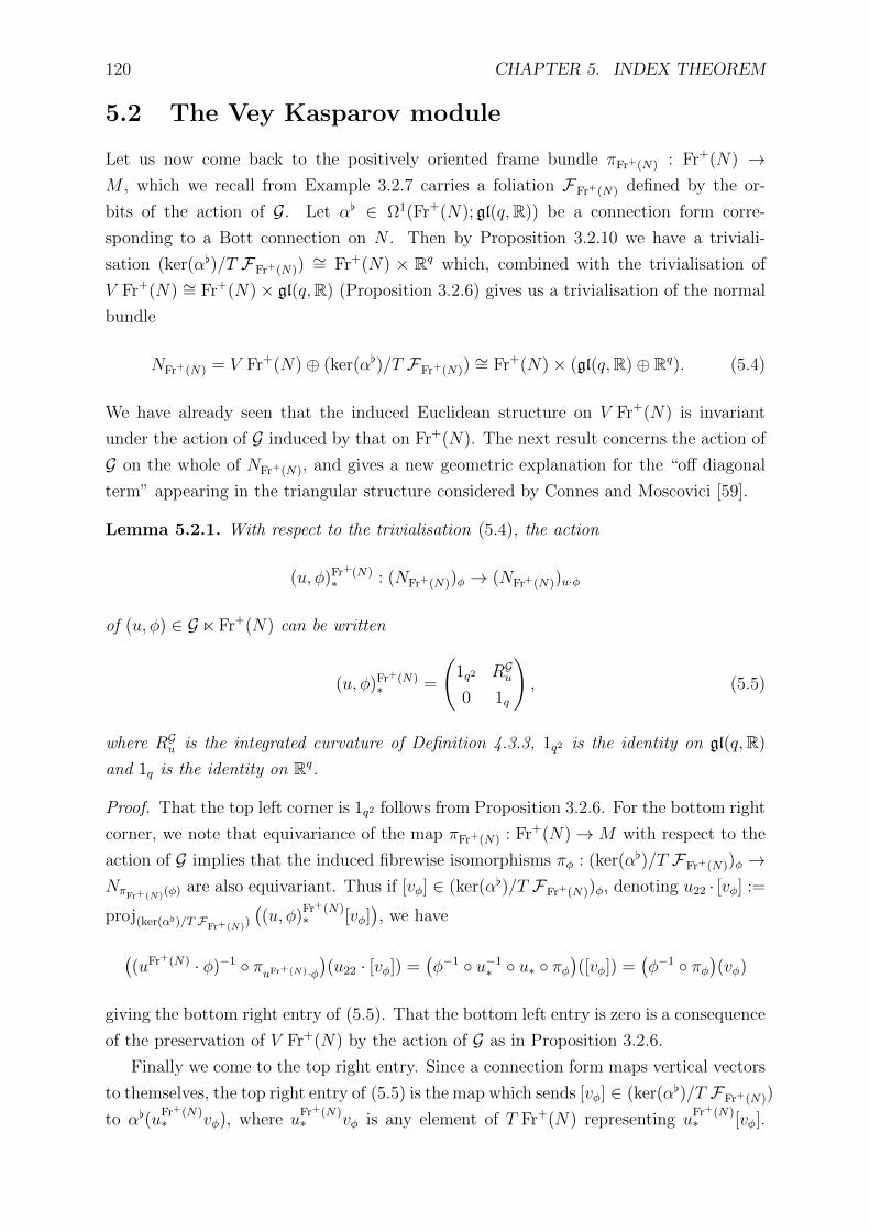
120 CHAPTER 5. INDEX THEOREM
5.2 The Vey Kasparov module
Let us now come back to the positively oriented frame bundle πFr+(N) : Fr+(N) →M , which we recall from Example 3.2.7 carries a foliation FFr+(N) defined by the or-
bits of the action of G. Let α[ ∈ Ω1(Fr+(N); gl(q,R)) be a connection form corre-
sponding to a Bott connection on N . Then by Proposition 3.2.10 we have a triviali-
sation (ker(α[)/T FFr+(N))∼= Fr+(N) × Rq which, combined with the trivialisation of
V Fr+(N) ∼= Fr+(N)× gl(q,R) (Proposition 3.2.6) gives us a trivialisation of the normal
bundle
NFr+(N) = V Fr+(N)⊕ (ker(α[)/T FFr+(N))∼= Fr+(N)× (gl(q,R)⊕ Rq). (5.4)
We have already seen that the induced Euclidean structure on V Fr+(N) is invariant
under the action of G induced by that on Fr+(N). The next result concerns the action of
G on the whole of NFr+(N), and gives a new geometric explanation for the “off diagonal
term” appearing in the triangular structure considered by Connes and Moscovici [59].
Lemma 5.2.1. With respect to the trivialisation (5.4), the action
(u, φ)Fr+(N)∗ : (NFr+(N))φ → (NFr+(N))u·φ
of (u, φ) ∈ GnFr+(N) can be written
(u, φ)Fr+(N)∗ =
(1q2 RGu
0 1q
), (5.5)
where RGu is the integrated curvature of Definition 4.3.3, 1q2 is the identity on gl(q,R)
and 1q is the identity on Rq.
Proof. That the top left corner is 1q2 follows from Proposition 3.2.6. For the bottom right
corner, we note that equivariance of the map πFr+(N) : Fr+(N)→ M with respect to the
action of G implies that the induced fibrewise isomorphisms πφ : (ker(α[)/T FFr+(N))φ →NπFr+(N)(φ) are also equivariant. Thus if [vφ] ∈ (ker(α[)/T FFr+(N))φ, denoting u22 · [vφ] :=
proj(ker(α[)/T FFr+(N))
((u, φ)
Fr+(N)∗ [vφ]
), we have
((uFr+(N) · φ)−1 πuFr+(N)·φ
)(u22 · [vφ]) =
(φ−1 u−1
∗ u∗ πφ)([vφ]) =
(φ−1 πφ
)(vφ)
giving the bottom right entry of (5.5). That the bottom left entry is zero is a consequence
of the preservation of V Fr+(N) by the action of G as in Proposition 3.2.6.
Finally we come to the top right entry. Since a connection form maps vertical vectors
to themselves, the top right entry of (5.5) is the map which sends [vφ] ∈ (ker(α[)/T FFr+(N))
to α[(uFr+(N)∗ vφ), where u
Fr+(N)∗ vφ is any element of T Fr+(N) representing u
Fr+(N)∗ [vφ].
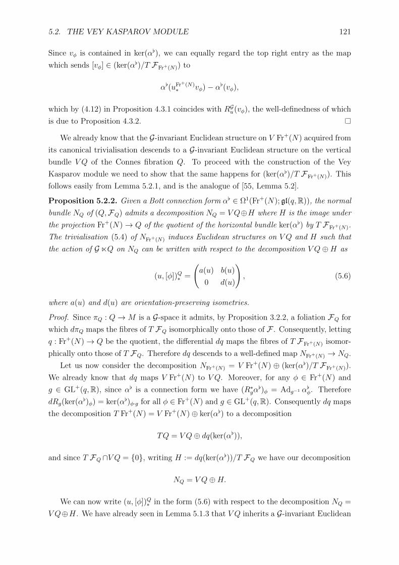
5.2. THE VEY KASPAROV MODULE 121
Since vφ is contained in ker(α[), we can equally regard the top right entry as the map
which sends [vφ] ∈ (ker(α[)/T FFr+(N)) to
α[(uFr+(N)∗ vφ)− α[(vφ),
which by (4.12) in Proposition 4.3.1 coincides with RGu(vφ), the well-definedness of which
is due to Proposition 4.3.2.
We already know that the G-invariant Euclidean structure on V Fr+(N) acquired from
its canonical trivialisation descends to a G-invariant Euclidean structure on the vertical
bundle V Q of the Connes fibration Q. To proceed with the construction of the Vey
Kasparov module we need to show that the same happens for (ker(α[)/T FFr+(N)). This
follows easily from Lemma 5.2.1, and is the analogue of [55, Lemma 5.2].
Proposition 5.2.2. Given a Bott connection form α[ ∈ Ω1(Fr+(N); gl(q,R)), the normal
bundle NQ of (Q,FQ) admits a decomposition NQ = V Q⊕H where H is the image under
the projection Fr+(N)→ Q of the quotient of the horizontal bundle ker(α[) by T FFr+(N).
The trivialisation (5.4) of NFr+(N) induces Euclidean structures on V Q and H such that
the action of GnQ on NQ can be written with respect to the decomposition V Q⊕H as
(u, [φ])Q∗ =
(a(u) b(u)
0 d(u)
), (5.6)
where a(u) and d(u) are orientation-preserving isometries.
Proof. Since πQ : Q→M is a G-space it admits, by Proposition 3.2.2, a foliation FQ for
which dπQ maps the fibres of T FQ isomorphically onto those of F . Consequently, letting
q : Fr+(N)→ Q be the quotient, the differential dq maps the fibres of T FFr+(N) isomor-
phically onto those of T FQ. Therefore dq descends to a well-defined map NFr+(N) → NQ.
Let us now consider the decomposition NFr+(N) = V Fr+(N) ⊕ (ker(α[)/T FFr+(N)).
We already know that dq maps V Fr+(N) to V Q. Moreover, for any φ ∈ Fr+(N) and
g ∈ GL+(q,R), since α[ is a connection form we have (R∗gα[)φ = Adg−1 α[φ. Therefore
dRg(ker(α[)φ) = ker(α[)φ·g for all φ ∈ Fr+(N) and g ∈ GL+(q,R). Consequently dq maps
the decomposition T Fr+(N) = V Fr+(N)⊕ ker(α[) to a decomposition
TQ = V Q⊕ dq(ker(α[)),
and since T FQ ∩V Q = 0, writing H := dq(ker(α[))/T FQ we have our decomposition
NQ = V Q⊕H.
We can now write (u, [φ])Q∗ in the form (5.6) with respect to the decomposition NQ =
V Q⊕H. We have already seen in Lemma 5.1.3 that V Q inherits a G-invariant Euclidean

122 CHAPTER 5. INDEX THEOREM
structure from the trivialisation (5.4), and this tells us that a(u) is indeed an orientation-
preserving isometry. For d(u), we let · denote the dot product on Rq, and for any choice
φ ∈ Fr+(N) representing [φ] ∈ Q we take dqφ to be the isomorphism
Rq ∼= (ker(α[)/T FFr+(N))φdqφ−−→ H[φ],
where Rq is identified with ker(α[)/T FFr+(N) as in Proposition 3.2.10. We then define
our Euclidean structure gH on H by
gH[φ](h1, h2) := (dq−1φ h1) · (dq−1
φ h2).
Since the dot product is invariant under special orthogonal transformations, gH is well-
defined. That d(u) is an orientation-preserving isometry now follows from the equivari-
ance of q and Equation (5.5) of Proposition 5.2.1.
Note that the elements of the matrix (5.6) will in general be dependent on [φ] as well
as u. This is true of all of the groupoid cocycles we will make use of later in the section.
We choose to omit the [φ] for notational simplicity. The triangular structure of the matrix
(5.6) will be used to construct a G-space for which the action of u ∈ G encodes Tr(RGu),
which is a path-integrated version of the first Pontryagin class of the normal bundle. For
this we need a lemma which tells us that the matrix trace gives a well-defined map on
V Q.
Lemma 5.2.3. Let TrV Fr+(N) : V Fr+(N)→ Fr+(N)×R be the vector bundle map defined
by
V Fr+(N) 3 V Xφ 7→ (φ,Tr(X)) ∈ Fr+(N)× R,
where V X is the fundamental vector field on Fr+(N) associated to X ∈ gl(q,R). Then,
recalling the diagonal element a(u) of the matrix in Equation (5.6), TrV Fr+(N) descends
to a well-defined vector bundle map TrV Q : V Q→ Q×R such that for all (u, [φ]) ∈ GnQone has TrV Q
uQ·[φ]a(u) = (uQ × idR) TrV Q[φ] as maps H[φ] → R.
Proof. For g ∈ GL+(q,R) and X ∈ gl(q,R) we have dRg(VXφ ) = V
Adg−1 X
φ·g . Since the
matrix trace is invariant under the adjoint action it follows that Tr does indeed descend
to a map TrV Q : V Q→ Q× R, defined explicitly for dqφ(V Xφ ) ∈ V[φ]Q by
TrV Q(dqφ(V Xφ )) := ([φ],Tr(X)).
The final assertion now follows from the equivariance of q: for any (u, [φ]) ∈ GnQ we
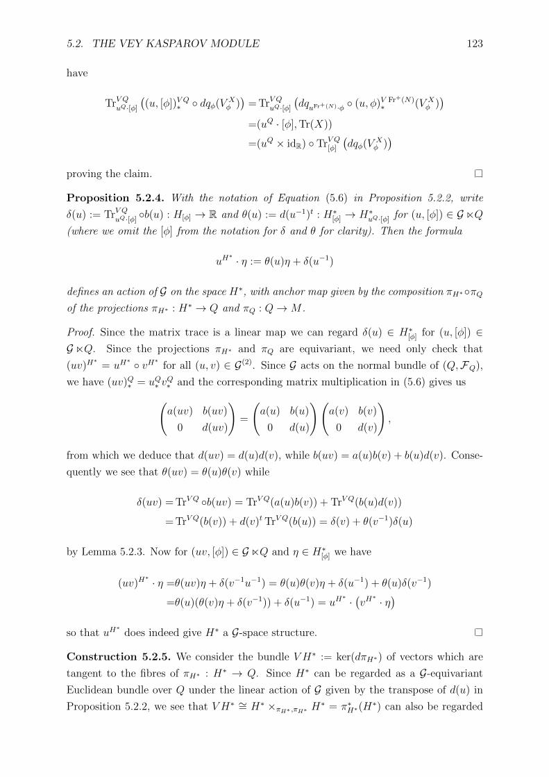
5.2. THE VEY KASPAROV MODULE 123
have
TrV QuQ·[φ]
((u, [φ])V Q∗ dqφ(V X
φ ))
= TrV QuQ·[φ]
(dquFr+(N)·φ (u, φ)V Fr+(N)
∗ (V Xφ ))
=(uQ · [φ],Tr(X))
=(uQ × idR) TrV Q[φ]
(dqφ(V X
φ ))
proving the claim.
Proposition 5.2.4. With the notation of Equation (5.6) in Proposition 5.2.2, write
δ(u) := TrV QuQ·[φ]
b(u) : H[φ] → R and θ(u) := d(u−1)t : H∗[φ] → H∗uQ·[φ] for (u, [φ]) ∈ GnQ(where we omit the [φ] from the notation for δ and θ for clarity). Then the formula
uH∗ · η := θ(u)η + δ(u−1)
defines an action of G on the space H∗, with anchor map given by the composition πH∗πQof the projections πH∗ : H∗ → Q and πQ : Q→M .
Proof. Since the matrix trace is a linear map we can regard δ(u) ∈ H∗[φ] for (u, [φ]) ∈GnQ. Since the projections πH∗ and πQ are equivariant, we need only check that
(uv)H∗
= uH∗ vH∗ for all (u, v) ∈ G(2). Since G acts on the normal bundle of (Q,FQ),
we have (uv)Q∗ = uQ∗ vQ∗ and the corresponding matrix multiplication in (5.6) gives us(a(uv) b(uv)
0 d(uv)
)=
(a(u) b(u)
0 d(u)
)(a(v) b(v)
0 d(v)
),
from which we deduce that d(uv) = d(u)d(v), while b(uv) = a(u)b(v) + b(u)d(v). Conse-
quently we see that θ(uv) = θ(u)θ(v) while
δ(uv) = TrV Q b(uv) = TrV Q(a(u)b(v)) + TrV Q(b(u)d(v))
= TrV Q(b(v)) + d(v)t TrV Q(b(u)) = δ(v) + θ(v−1)δ(u)
by Lemma 5.2.3. Now for (uv, [φ]) ∈ GnQ and η ∈ H∗[φ] we have
(uv)H∗ · η =θ(uv)η + δ(v−1u−1) = θ(u)θ(v)η + δ(u−1) + θ(u)δ(v−1)
=θ(u)(θ(v)η + δ(v−1)) + δ(u−1) = uH∗ ·(vH∗ · η
)so that uH
∗does indeed give H∗ a G-space structure.
Construction 5.2.5. We consider the bundle V H∗ := ker(dπH∗) of vectors which are
tangent to the fibres of πH∗ : H∗ → Q. Since H∗ can be regarded as a G-equivariant
Euclidean bundle over Q under the linear action of G given by the transpose of d(u) in
Proposition 5.2.2, we see that V H∗ ∼= H∗ ×πH∗ ,πH∗ H∗ = π∗H∗(H∗) can also be regarded

124 CHAPTER 5. INDEX THEOREM
as a G-equivariant Euclidean bundle over the G-space H∗ equipped with the G-action of
Proposition 5.2.4. More specifically, for (u, [φ]) ∈ GnQ we obtain the G-vector bundle
structure of V H∗ by the formula
uV H∗
∗ (η1, η2) :=(uH∗ · η1, d(u−1)tη2
)=(θ(u)η1 + δ(u−1), θ(u)η2
)for (η1, η2) ∈ H∗ ×πH∗ ,πH∗ H∗, where the second factor of H∗ is equipped with the Eu-
clidean structure inherited from that of H in Proposition 5.2.2 under which d(u), and
therefore θ(u), is orthogonal and orientation-preserving.
Consequently, the algebra C`H∗(V H∗) of sections vanishing at infinity of the Clifford
algebra bundle Cliff(V H∗) → H∗ is a G-algebra, where for (u, [φ]) ∈ GnQ the action
βu : C`H∗(V H∗)s(u) → C`H∗(V H∗)r(u) is defined on σ ∈ C`H∗(V H∗)s(u) by
βu(σ)(η) := uV H∗
c σ(θ(u−1)η + δ(u)
), η ∈ H∗[φ].
We regard the G-algebra C`H∗(V H∗) as a G-equivariant Hilbert module over itself in the
usual way, and define a representation ν of the G-algebra C0(Q) thereon by the formula
ν(g)σ(η) := g(πH∗(η))σ(η), η ∈ H∗
where equivariance of the projection πH∗ : H∗ → Q guarantees that ν is a G-equivariant
representation.
Finally, we define an operator B2 on sections σ contained in the dense submodule
Γc(H∗;Cliff(V H∗)) of C`H∗(V H∗) by the formula
(B2σ)(η) := η · σ(η), η ∈ H∗,
where · denotes Clifford multiplication in the fibres of Cliff(V H∗). We will now show
that the triple (C0(Q), ν C`H∗(V H∗), B2) is a Kasparov module.
Proposition 5.2.6. The triple (C0(Q), ν C`H∗(V H∗), B2) is an unbounded, G-equivariant
Kasparov C0(Q)-C`H∗(V H∗)-module, so defines a class [B2] ∈ KKG(C0(Q),C`H∗(V H∗)).
Proof. That B2 is essentially self-adjoint and regular follows from the same argument
as in the proof of Proposition 5.1.6. The operator B2 moreover commutes with the
representation ν of C0(Q), and has locally compact resolvent by the same argument as
in Proposition 5.1.6.
All that remains to check is that B2 is appropriately equivariant. For this, we take

5.2. THE VEY KASPAROV MODULE 125
u ∈ G and σ ∈ Γc(H∗;Cliff(V H∗)), and for η ∈ H∗[φ] with [φ] ∈ Qr(u) we calculate
(βu B2 βu−1)σ(η) =uV H∗
c
((B2 βu−1)σ
)(θ(u−1)η + δ(u))
=uV H∗
c
((θ(u−1)η + δ(u)) · (βu−1σ)(θ(u−1)η + δ(u))
)=uV H
∗
c
((θ(u−1)η + δ(u)) · (u−1)V H
∗
c σ(η))
=(η − δ(u−1)) · σ(η),
from which we deduce that
(B2 − βu B2 βu−1)σ(η) = δ(u−1) · σ(η).
Now smoothness of the map u 7→ δ(u−1) implies that for any f ∈ C0(Q), any Hausdorff
open subset U of G and any ϕ ∈ Cc(U) we have
ϕ · νrU(r∗U(f)) ·(r∗U(B2)− βU s∗U(B2) β−1
U
)∈ L(r∗U C`H∗(V H∗)),
and therefore we conclude that (C0(Q), ν C`H∗(V H∗), B2) is an unbounded, G-equivariant
Kasparov C0(Q)-C`H∗(V H∗)-module.
Definition 5.2.7. The Kasparov module of Proposition 5.2.6 will be referred to as the
Vey Kasparov module.
Remark 5.2.8. In order to justify our terminology, let us recall briefly the Vey homo-
morphism of [97, 68]. Choosing a transverse volume form ω ∈ Ωq(M) for (M,F), we
let A(M,F) denote the differential ideal in Ω(M) generated by ω. If R[ is the curva-
ture of any Bott connection on N , then by the argument of the Bott vanishing theorem
(Theorem 2.4.18), for each element c ∈ I∗q (R) = R[c1, . . . , cq] of degree 2q, (see Def-
inition 2.4.19), we have that c(R[) ∈ A(M,F). The Vey homomorphism is the map
V (c) : Ω(M)→ A(M,F) defined by
V (c)(ψ) := ψ ∧ c(R[).
The Vey homomorphism can be thought of as one “half” of the Godbillon-Vey invariant,
in the sense that given η ∈ Ω1(M) for which dω = η∧ω we have V (cq1)(η) = η∧(dη)q = gv
for an appropriate choice of connection as in Theorem 2.5.4.
By Propositions 5.2.1 and 5.2.2, for u ∈ G our Kasparov module encodes in its equiv-
ariant structure the operator
Bu2 := B2 − βu B2 β−1
u = δ(u−1)· = c1(RGu−1)·
on C`H∗(V H∗), where the · denotes Clifford multiplication. As we will see later in

126 CHAPTER 5. INDEX THEOREM
this chapter, in codimension 1 the operator Bu2 appears in the local index formula for a
semifinite spectral triple constructed fromB2 and gives rise to the Godbillon-Vey groupoid
cocycle
αG ∧ c1(RG) = αG ∧RG
considered in Definition 4.3.6. We think of αG ∧ RG as an “integrated version” of
V (c1)(αG), sitting now over the frame bundle of N rather than on the base M . Hence
the terminology “Vey Kasparov module”.
The codimension 1 case is of course somewhat degenerate, and unfortunately it is far
from clear that the higher codimension Vey Kasparov module can be used to compute
the higher codimension Godbillon-Vey invariant. The fact that c1(RG) was used in the
construction of the Vey Kasparov module (as opposed to any of the other ci) suggests
that the scope of application of the Vey Kasparov module may be rather limited.
5.3 An index theorem for the Godbillon-Vey cyclic
cocycle
Let us now suppose that (M,F) is of codimension 1. We will recover the Godbillon-Vey
cyclic cocycle of Proposition 4.3.6 as the Chern character of a semifinite spectral triple
built from the Vey Kasparov module of Proposition 5.2.6.
5.3.1 The spectral triple
When (M,F) is of codimension 1, we can greatly simplify the Vey Kasparov module by
a choice of transverse volume form ω ∈ Ω1(M) (see Definition 2.3.2). The form ω is
associated with a (normal) vector field Z such that ω(Z) is everywhere equal to 1, and
this Z determines the following trivialisations.
1. N 3 nZx 7→ (x, n) ∈ M × R. The modular function ∆ : G → R∗+ defined by the
equation
r∗ω = ∆ s∗ω
(see Definition 4.3.10) then allows us to write the action u∗ : Ns(u) → Nr(u) of u ∈ Gin this trivialisation as
u∗(s(u), n) = (r(u),∆(u)n), n ∈ R .
2. Q 3 φ 7→ (πQ(φ), tφ) ∈ M × R∗+, where tφ ∈ R∗+ is defined by the equation φ(1) =
tφZπQ(φ), in which u ∈ G acts by
uQ · (s(u), t) = (r(u),∆(u)t), t ∈ R∗+ .

5.3. AN INDEX THEOREM FOR THE GODBILLON-VEY CYCLIC COCYCLE 127
3. H ∼= Q×R = M ×R∗+×R, arising from the trivialisation N ∼= M ×R induced by
Z together with the identification H ∼= π∗QN implied by the fact that dπQ induces
a fibrewise isomorphism of H onto N . The Euclidean structure on H discussed in
Proposition 5.2.2 is now given by
gH(x,t)(h1, h2) := t−2h1h2, (x, t) ∈M × R∗+, h1, h2 ∈ H(x,t) = R .
We use this gH to identify h ∈ H(x,t) with η = gH(x,t)(h, ·) ∈ H∗(x,t) - that is, h ∈ H(x,t)
identifies with ηh = t−2h ∈ R. The resulting Euclidean structure on H∗ is given by
gH∗
(x,t)(ηh, ηh′) := gH(x,t)(h, h′) = t−2hh′ = t2ηhηh′ ,
while the G-space structure on H∗ of Proposition 5.2.4 can be written
uH∗ · (s(u), t, η) = (r(u),∆(u)t,∆(u−1)η + δ(u−1)),
where δ : G1 → R is the function defined by Equation (4.13).
There is one further trivialisation that is not induced by Z and which will be necessary
in simplifying the Vey Kasparov module. Namely, we trivialise V H∗ = H∗ ×πH∗ ,πH∗ H∗
by the formula
κ(x, t, η1, η2) := (x, t, η1, tη2), (x, t, η1, η2) ∈ V H∗,
which arises from the status of Q = Fr+(N) as the frame bundle of N . Because
∆(u)t∆(u−1)η2 = tη2, G acts as the identity on the fibres of V H∗ in this trivialisa-
tion. We can therefore replace the G-algebra C`H∗(V H∗) that appears as the right-hand
algebra of the Vey Kasparov module with the G-algebra C0(H∗) ⊗ Cliff(R), where G is
the identity on the Cliff(R) factor and acts on C0(H∗) by
βu(f)(r(u), t, η) = f(s(u),∆(u−1)t,∆(u)η + δ(u))
for u ∈ G, and (t, η) ∈ R∗+×R ∼= H∗|Qr(u). Redefine ν to be a representation of C0(Q) on
C0(H∗) in which for a ∈ C0(Q) and g ∈ C0(H∗) one has
ν(a)(g)(x, t, η) := a(x, t)g(x, t, η), (x, t, η) ∈ H∗,
and redefine B2 to act on functions f in the dense submodule Cc(H∗) of C0(H∗) by the
formula
B2f(x, t, η) := tη f(x, t, η), (x, t, η) ∈ H∗.
Using [56, Proposition 13, Appendix A, Chapter 4] to obtain an odd Kasparov module

128 CHAPTER 5. INDEX THEOREM
by dropping the Cliff(R), we have the following.
Proposition 5.3.1. The Vey Kasparov module can, in codimension 1, be regarded as
the unbounded G-equivariant Kasparov module (C0(Q), νC0(H∗)⊗Cliff(R), B2). Applying
Kasparov’s descent map (see Proposition B.7.6, replacing “continuous” with “smooth”)
gives us an odd, unbounded Kasparov C∗r (Qo G)-C∗r (H∗ o G)-module
(C∞c (Qo G; Ω12 ), νC
∞c (H∗ o G; Ω
12 ),B)
defining a class [B] ∈ KK1(C0(Q) or G, C0(H∗) or G).
We consider now the forms
ωQ(x,t) := t−2ωx ∧ dt
and
ωH∗
(x,t,η) := t−1ωx ∧ dt ∧ dη (5.7)
on Q and H∗ respectively. It is easily verified that these forms are invariant under the
action of G on their respective underlying spaces, hence define traces τQ and τH∗ on
C∞c (Qo G; Ω12 ) and C∞c (H∗ o G; Ω
12 ) respectively.
Putting the trace τH∗ together with the odd Kasparov module of Proposition 5.3.1,
by Proposition A.1.36 we obtain an odd semifinite spectral triple
(A,H,B)
relative to (N , τ) where:
1. A = C∞c (Qo G; Ω12 ) acts by convolution operators on
2. H, the Hilbert space completion of C∞c (H∗ o G; Ω12 ) in the inner product
(ρ1|ρ2) = τH∗(ρ∗1 ∗ ρ2),
3. B is regarded as an operator on H with domain C∞c (H∗ o G; Ω12 ),
4. N is the weak closure of C∞c (H∗ o G; Ω12 ) in the bounded operators on H and,
5. τ is the normal extension of τQ to N .
We now apply the semifinite local index formula to (A,H,B) to prove the codimension
1 Godbillon-Vey index theorem.

5.3. AN INDEX THEOREM FOR THE GODBILLON-VEY CYCLIC COCYCLE 129
5.3.2 The index theorem
We will apply the residue cocycle of Definition A.2.12 to prove the following theorem.
Theorem 5.3.2. Let (M,F) be a transversely orientable foliated manifold of codimension
1. The Chern character of the semifinite spectral triple (A,H,B) given in Section 5.3.1
coincides up to a factor of (2πi)12 with the Godbillon-Vey cyclic cocycle (4.15).
To apply the local index formula we need to check the summability and smoothness
of the spectral triple.
Lemma 5.3.3. The spectral triple (A,H,B) is smoothly summable of spectral dimension
p = 1 and has isolated spectral dimension.
Proof. Let us first recall the notational convention of Example B.6.8, where for a G-space
Y and for f ∈ C∞c (Y o G; Ω12 ), we use the notation
fu(y) := f(y, u) (y, u) ∈ Y o G,
to emphasise that the groupoid variable and the fibre variables are playing distinct roles.
The variables (x, t, η) will always be used to denote points in H∗.
We check finite summability. For s ∈ R, a ∈ C∞c (Qo G; Ω12 ) and ρ ∈ H, we calculate
(a(1+B2)−s2ρ)u(x, t, η) =
∫v∈Gr(u)
av(x, t)(βv(1 + B2
s(v))− s
2ρv−1u)(x, t, η)
=
∫v∈Gr(u)
av(x, t)(1 + t2∆(v−1)2(∆(v)η + δ(v))2)−s2 (βvρv−1u)(x, t, η)
=
∫v∈Gr(u)
av(x, t)(1 + t2(η − δ(v−1))2)−s2 (βvρv−1u)(x, t, η),
where on the last line we have simplified ∆(v−1)δ(v) = −δ(v−1) using Equation (4.14).
So a(1 + B2)−s2 is the half-density on H∗ o G defined by
((x, t, η), u) 7→ au(x, t)(1 + t2(η − δ(u−1))2
)− s2 ,
compactly supported in the u and (x, t) variables. Thus, since τH∗ is defined by integration
over the unit space H∗ of H∗ o G, we have
τH∗(a(1 + B2)−s2 ) =
∫M×R∗+×R
a(x, t)(1 + t2η2
)− s2 t−1ω ∧ dt ∧ dη
=
∫Q
a(x, t)dνQ
∫R
(1 + η2
)− s2dη,
where we have made the substitution η = tη. It is then clear that τH∗(a(1 + B2)−s2 ) is
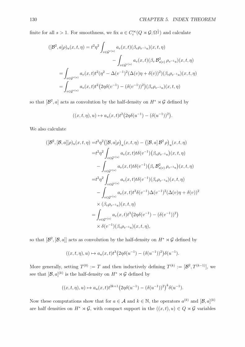
130 CHAPTER 5. INDEX THEOREM
finite for all s > 1. For smoothness, we fix a ∈ C∞c (Qo G; Ω12 ) and calculate
([B2, a]ρ)u(x, t, η) = t2η2
∫v∈Gr(u)
av(x, t)(βvρv−1u)(x, t, η)
−∫v∈Gr(u)
av(x, t)(βv B2s(v) ρv−1u)(x, t, η)
=
∫v∈Gr(u)
av(x, t)t2(η2 −∆(v−1)2(∆(v)η + δ(v))2)(βvρv−1u)(x, t, η)
=
∫v∈Gr(u)
av(x, t)t2(2ηδ(v−1)− (δ(v−1))2
)(βvρv−1u)(x, t, η)
so that [B2, a] acts as convolution by the half-density on H∗ o G defined by
((x, t, η), u) 7→ au(x, t)t2(2ηδ(u−1)− (δ(u−1))2
).
We also calculate
([B2, [B, a]]ρ)u(x, t, η) =t2η2([B, a]ρ
)u(x, t, η)−
([B, a]B2 ρ
)u(x, t, η)
=t2η2
∫v∈Gr(u)
av(x, t)tδ(v−1)(βvρv−1u
)(x, t, η)
−∫v∈Gr(u)
av(x, t)tδ(v−1)(βv B2
s(v) ρv−1u
)(x, t, η)
=t2η2
∫v∈Gr(u)
av(x, t)tδ(v−1)(βvρv−1u)(x, t, η)
−∫v∈Gr(u)
av(x, t)t3δ(v−1)∆(v−1)2(∆(v)η + δ(v))2
× (βvρv−1u)(x, t, η)
=
∫v∈Gr(u)
av(x, t)t3(2ηδ(v−1)− (δ(v−1))2
)× δ(v−1)(βvρv−1u)(x, t, η),
so that [B2, [B, a]] acts as convolution by the half-density on H∗ o G defined by
((x, t, η), u) 7→ au(x, t)t3(2ηδ(u−1)− (δ(u−1))2
)δ(u−1).
More generally, setting T (0) := T and then inductively defining T (k) := [B2, T (k−1)], we
see that [B, a](k) is the half-density on H∗ o G defined by
((x, t, η), u) 7→ au(x, t)t2k+1
(2ηδ(u−1)− (δ(u−1))2
)kδ(u−1).
Now these computations show that for a ∈ A and k ∈ N, the operators a(k) and [B, a](k)
are half densities on H∗ o G, with compact support in the ((x, t), u) ∈ Q o G variables
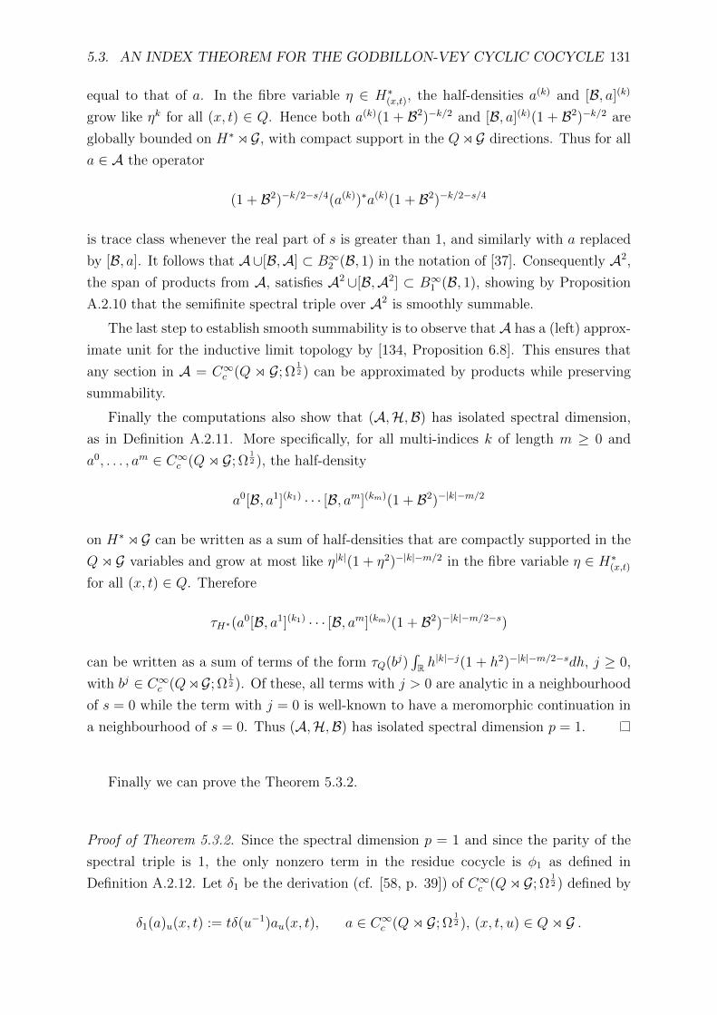
5.3. AN INDEX THEOREM FOR THE GODBILLON-VEY CYCLIC COCYCLE 131
equal to that of a. In the fibre variable η ∈ H∗(x,t), the half-densities a(k) and [B, a](k)
grow like ηk for all (x, t) ∈ Q. Hence both a(k)(1 + B2)−k/2 and [B, a](k)(1 + B2)−k/2 are
globally bounded on H∗oG, with compact support in the QoG directions. Thus for all
a ∈ A the operator
(1 + B2)−k/2−s/4(a(k))∗a(k)(1 + B2)−k/2−s/4
is trace class whenever the real part of s is greater than 1, and similarly with a replaced
by [B, a]. It follows that A∪[B,A] ⊂ B∞2 (B, 1) in the notation of [37]. Consequently A2,
the span of products from A, satisfies A2 ∪[B,A2] ⊂ B∞1 (B, 1), showing by Proposition
A.2.10 that the semifinite spectral triple over A2 is smoothly summable.
The last step to establish smooth summability is to observe that A has a (left) approx-
imate unit for the inductive limit topology by [134, Proposition 6.8]. This ensures that
any section in A = C∞c (Q o G; Ω12 ) can be approximated by products while preserving
summability.
Finally the computations also show that (A,H,B) has isolated spectral dimension,
as in Definition A.2.11. More specifically, for all multi-indices k of length m ≥ 0 and
a0, . . . , am ∈ C∞c (Qo G; Ω12 ), the half-density
a0[B, a1](k1) · · · [B, am](km)(1 + B2)−|k|−m/2
on H∗o G can be written as a sum of half-densities that are compactly supported in the
Qo G variables and grow at most like η|k|(1 + η2)−|k|−m/2 in the fibre variable η ∈ H∗(x,t)for all (x, t) ∈ Q. Therefore
τH∗(a0[B, a1](k1) · · · [B, am](km)(1 + B2)−|k|−m/2−s)
can be written as a sum of terms of the form τQ(bj)∫R h|k|−j(1 + h2)−|k|−m/2−sdh, j ≥ 0,
with bj ∈ C∞c (QoG; Ω12 ). Of these, all terms with j > 0 are analytic in a neighbourhood
of s = 0 while the term with j = 0 is well-known to have a meromorphic continuation in
a neighbourhood of s = 0. Thus (A,H,B) has isolated spectral dimension p = 1.
Finally we can prove the Theorem 5.3.2.
Proof of Theorem 5.3.2. Since the spectral dimension p = 1 and since the parity of the
spectral triple is 1, the only nonzero term in the residue cocycle is φ1 as defined in
Definition A.2.12. Let δ1 be the derivation (cf. [58, p. 39]) of C∞c (Qo G; Ω12 ) defined by
δ1(a)u(x, t) := tδ(u−1)au(x, t), a ∈ C∞c (Qo G; Ω12 ), (x, t, u) ∈ Qo G .

132 CHAPTER 5. INDEX THEOREM
Then for any a ∈ C∞c (Qo G; Ω12 ) we have
([B, a]ρ
)u(x, t, η) =Br(u)
∫v∈Gr(u)
av(x, t)(βvρv−1u)(x, t, η)
−∫v∈Gr(u)
av(x, t)(βv Bs(v) ρv−1u)(x, t, η)
=
∫v∈Gr(u)
av(x, t)(Br(v)−βv Bs(v) βv−1
)(βvρv−1u)(x, t, η)
=
∫v∈Gr(u)
av(x, t)tδ(v−1)(βvρv−1u)(x, t, η)
=(δ1(a)ρ)u(x, t, η).
Thus for a0, a1 ∈ C∞c (Qo G; Ω12 ), we calculate
φ1(a0, a1) =2(2πi)12 resz=0 τH∗
(a0[B, a1](1 + B2)−
12−z)
=2(2πi)12 τQ(a0δ1(a1)) resz=0
∫R(1 + h2)−
12−zdh.
Letting Γ denote the Gamma function we obtain
φ1(a0, a1) =2(2πi)12 τQ(a0δ1(a1)) resz=0
Γ(1/2)Γ(z)
2Γ(1/2 + z)
=(2πi)12 τQ(a0δ1(a1))
=(2πi)12
∫(x,t)∈M×R∗+
∫u∈Gx
a0u(x, t)
(δ1a
1)u−1(u−1 · x,∆(u−1)t)
1
t2ωx ∧ dt
=(2πi)12
∫(x,t)∈M×R∗+
∫u∈Gx
a0u(x, t)a
1u−1(u−1 · x,∆(u−1)t)
∆(u−1)tδ(u)
t2ωx ∧ dt
=− (2πi)12
∫(x,t)∈M×R∗+
∫u∈Gx
a0u(x, t)a
1u−1(u−1 · x,∆(u−1)t)
δ(u−1)
tωx ∧ dt,
where we have again made use of the identity (4.14) in going from the penultimate line to
the last. This is, up to the factor (2πi)12 , the Godbillon-Vey cyclic cocycle of (4.15).
Remark 5.3.4. Let us briefly remark now that our semifinite spectral triple can really be
regarded as the non-etale analogue of the construction given by Connes in [55, Theorem
7.15]. Connes works with an oriented manifold V acted on by a discrete group Γ of
diffeomorphisms. Let us assume that V is 1-dimensional and denote by J+k the kth-order
jet bundle of V . Connes constructs an explicit Kasparov module T1 defining a class in
KK1Γ(C0(V ), C0(J+
1 )), which is the etale analogue of, and the inspiration for, the Connes
Kasparov module constructed in this thesis. Connes then uses the fact that the fibres of
J+2 → J+
1 are nilpotent Lie groups together with the work of Kasparov [74] to infer that
there is an equivariant class [T2] ∈ KK1Γ(C0(J+
1 ), C0(J+2 )) (although he does not construct
the module explicitly). The Godbillon-Vey invariant defines a Γ-invariant 3-form on J+2

5.3. AN INDEX THEOREM FOR THE GODBILLON-VEY CYCLIC COCYCLE 133
in a similar manner to Corollary 3.2.34, and therefore a trace τ on C∞c (J+2 oΓ) . Connes
computes the map K0(C∗r (V o Γ))→ R given by
K0(C∗r (V o Γ)) 3 x 7→ τ(x⊗C∗r (V oΓ) [T1]⊗C∗r (J+
1 oΓ) [T2])∈ R
as a cyclic cocycle on C∞c (V oΓ), obtaining his Godbillon-Vey cyclic cocycle [55, Theorem
7.3].
Coming back to the setting of a transversely orientable foliated manifold (M,F) of
codimension 1, recall from Definition 3.2.19 that associated to (M,F) are transverse
jet bundles J+k (F). Consider now Proposition 3.2.33, which identifies J+
2 (F) with the
horizontal normal bundle H on Q defined by a choice of torsion-free Bott connection on
N . Using the tautological Euclidean structure on H of Proposition 5.2.2, we can identify
J+2 (F) with H∗. Then the class in KK1(C∗r (Q o G), C∗r (H∗ o G)) defined by our Vey
Kasparov module is the non-etale analogue of the class in KK1(C∗r (J+1 oΓ), C∗r (J+
2 oΓ))
used by Connes. Note that in contrast with Connes’ approach, the class we obtain is
represented by an explicit Kasparov module, determined by the choice of Bott connection.
Note moreover that the G-invariant Godbillon-Vey form
gv =1
t3ω ∧ dt ∧ dh
on H of Proposition 3.2.34 is precisely the G-invariant form ωH∗
of Equation (5.7) under
the identification H(x,t) 3 h 7→ η := t−2h ∈ H∗(x,t) of H with H∗ induced by the met-
ric. Thus Theorem 5.3.2 can be viewed as an application of new tools (non-Hausdorff
groupoid-equivariant KK-theory and the semifinite local index formula) to an old prob-
lem solved by Connes.
Remark 5.3.5. It is tempting to take the Kasparov product of the Connes and Vey
Kasparov modules so as to obtain a semifinite spectral triple for the algebra C∞c (G; Ω12 ).
One would expect to recover a formula analogous to that of Connes [55, Theorem 7.3]
from the local index formula of this semifinite spectral triple.
In codimension 1, one can simplify the Connes Kasparov module to an odd equivariant
Kasparov C0(M)-C0(Q) module in a similar way to how the Vey Kasparov module is
simplified to an odd Kasparov module. The Kasparov product of the Connes and Vey
Kasparov modules is then quite easy to compute, due to the fact that the operators B1
and B2 used in their constructions commute with the actions of their respective left hand
algebras. Unfortunately, however, the semifinite spectral triple one obtains by applying
Proposition A.1.36 to the resulting product module with the trace τH∗ is not finitely
summable.
More specifically, writing Q = M × R∗+ and H∗ = M × R∗+×R with respect to the

134 CHAPTER 5. INDEX THEOREM
choice of transverse volume form ω, we recall that B2 acts on f ∈ C∞c (H∗) by
B2f(x, t, η) = tη f(x, t, η), (x, t, η) ∈ H∗
while B1 acts on g ∈ C∞c (Q) by
B1g(x, t) = log(t)g(x, t), (x, t) ∈ Q.
Then setting B := B1 ⊗ 1 + 1 ⊗ B2, we have that B2 = B21 ⊗ 1 + 1 ⊗ B2
2 acts on
f ∈ C∞c (Q)⊗C∞0 (Q) C∞c (H∗) = C∞c (H∗) by
B2f(x, t, η) = (log(t)2 + t2η2) f(x, t, η), (x, t, η) ∈ H∗.
Consequently for a ∈ C∞c (G; Ω12 ) and s > 0 we have
τH∗(a(1 +B2)−s2 ) =
∫(x,t,η)∈H∗
a(x)(1 + log(t)2 + t2η2)−
s2 t−1ωx ∧ dt ∧ dη.
Taking c := log(t) and η := ecη, the integral becomes
τH∗(a(1 +B2)−s2 ) =
∫(x,c,η)∈H∗
a(x)(1 + c2 + η2)−s2 e−cωx ∧ dc ∧ dη.
Since ec blows up faster as c goes to infinity than any polynomial, τH∗(a(1 + B2)−s2 )
cannot be finite for any s.
We remark that this is the same sort of phenomenon exhibited in [44], where a modular
spectral triple is used to compute a non-finitely summable semifinite index pairing for
the Cuntz algebra. In this case, one replaces the trace used for the semifinite index
pairing with a particular weight, with respect to which the resolvent of the operator
under consideration becomes finitely summable. One sees in our own setting that if one
were to replace the trace τH∗ on C∞c (H∗oG) determined by the form t−1ω∧ dt∧ dη with
the weight φ determined by ω ∧ dt ∧ dη, then using the same substitutions as with τH∗
we would have
φ(a(1 +B2)−s2 ) =
∫(x,c,η)∈H∗
a(x)(1 + log(t)2 + t2η2)−s2ωx ∧ dt ∧ dη
=
∫(x,c,η)∈H∗
a(x)(1 + c2 + η2)−s2ωx ∧ dc ∧ dη,
which is finite for all s > 2. While the foliation setting of a non-compact, locally Hausdorff
groupoid action is much more general than the circle action considered in [44], the parallels
in summability between the two settings suggest that perhaps modular spectral triples
could be generalised to the foliation setting so as to retain finite summability.

5.3. AN INDEX THEOREM FOR THE GODBILLON-VEY CYCLIC COCYCLE 135
Remark 5.3.6. Let us conclude this chapter with a final remark on the potential of the
higher codimension Vey Kasparov module for use in a higher codimension Godbillon-Vey
spectral triple. To construct a semifinite spectral triple from the Vey Kasparov module
one must choose a trace on the algebra C`H∗(V H∗) o G, for which there is an obvious
choice. Choose a transverse volume form ω on M . Take the G-invariant volume form
ωQ along the fibres of the Connes fibration Q determined by the canonical G-invariant
Euclidean structure on V Q as in Lemma 5.1.3, together with the (ungraded) Clifford
trace TrCliff in the fibres of Cliff(V H∗) over H∗ and the G-invariant volume form ωH∗
along the fibres of H∗ over Q. Moreover for [φ] ∈ Q = Fr+(N)/ SO(q,R) let det([φ])
denote the determinant of the frame φ. Then the functional
τ(ρ) :=
∫H∗
1
det([φ])TrCliff
(ρ(η[φ])
)ω ∧ ωQ ∧ ωH∗ ρ ∈ Γ∞c (H∗ o G;Cliff(V H∗)⊗ Ω
12 )
(5.8)
defines a trace on C`H∗(V H∗) that generalises the trace τH∗ used in codimension 1. One
might hope that combining τ with the Vey Kasparov module would produce a semifinite
spectral triple for the higher codimension Godbillon-Vey invariant, but there are a number
of problems with this hypothesis.
To see these problems let us first recall Bott’s formula for the Godbillon-Vey invariant
as a diffeomorphism group-cocycle. Bott [26, Equation 2] takes an oriented Riemannian
manifold V of dimension q, with Riemannian volume form θ, acted on by a discrete group
Γ of diffeomorphisms. For g ∈ Γ he defines µ(g) by the equation g∗θ = µ(g)θ, and if ∇is the Levi-Civita connection on V one has Tr(g∗∇−∇) = dµ(g). Bott’s Godbillon-Vey
group cocycle is then given by the formula
gv(g1, . . . , gq+1) =
∫V
log µ(f1) d log µ(f1f2) · · · d log µ(f1 · · · fq+1)
(cf. Crainic and Moerdijk’s [64, Corollary 3]). Let us call the string of d log µ(f)’s
the “Pontryagin part” of the cocycle, since as we have seen in Definition 4.3.3, each
d log µ(f) = Tr(g∗∇ − ∇) corresponds in the non-etale setting to the trace of a path-
integrated Bott curvature form. Let us also isolate the log µ(f) term and refer to it as the
“secondary part”. As discussed in Remark 5.2.8, the Vey Kasparov module contains the
correct representation-theoretic information for the “Pontryagin part” of the Godbillon-
Vey cocycle. On the other hand, however, the Connes Kasparov module encodes in its
own equivariant structure the entire SO(q,R)-equivalence class of the Jacobian of each
holonomy transport map, while the “secondary part” of the Godbillon-Vey cocycle involves
only the SL(q,R)-equivalence class, namely the determinant, of each holonomy transport
map.
All this is to say that while the equivariant structure of the Vey Kasparov module
is well-suited to the higher codimension Godbillon-Vey invariant (indeed, its construc-

136 CHAPTER 5. INDEX THEOREM
tion was motived precisely by the formulae obtained by Bott and Crainic-Moerdijk), the
equivariant structure of the Connes Kasparov module is much too large. One poten-
tial way around this problem, suggested by G. Skandalis, would be to replace the space
Q = Fr+(N)/ SO(q,R) of the Connes Kasparov module with the space Fr+(N)/ SL(q,R).
The issue with this approach, however, is that in doing so one loses the tautological
G-invariant Euclidean structure on the horizontal normal bundle (see Proposition 5.2.2)
that we exploited to construct the Vey Kasparov module. Due to the great difficulty of
constructing equivariant Kasparov modules without an invariant metric structure, this
approach appears to be unworkable.
Another potential solution might be to replace the q(q+1)2
-form ωQ in the Equation
(5.8) with the G-invariant 1-form
(ωQ)[φ] =1
det([φ])d(det([φ])), [φ] ∈ Q
along the fibres of Q. Clearly ωQ picks out precisely the determinant information that we
are after, and one might hope that by using ωQ in the place of ωQ we could construct a
cyclic cocycle on C`H∗(V H∗)oG to replace the trace τ . However, as we remarked at the
start of Section 4.3 in Chapter 4, the apparent absence of a transverse exterior derivative
in the non-etale case makes the identification of an appropriate cyclic cocycle from ωQ at
this stage impossible.
Appendix A
Noncommutative index theory
This appendix serves as a review of the basic noncommutative index theory required
for the final chapters of the thesis. As this material is really the bread and butter of
noncommutative index theory (and would take a whole separate thesis to flesh out in
complete detail), we refer to the well-known literature on the topic for proofs and details.
A.1 Index pairings and KK-theory
We describe in this section the bivariant K-theory of Kasparov, or simply KK-theory.
Kasparov’s original description of the theory [104] is now often referred to as the “bounded
picture” of KK-theory, as it deals with bounded operators only. Since the operators
that typically appear in classical index theory are unbounded (for instance the Dirac
operator on a Spin manifold), an unbounded picture of Kasparov’s theory was introduced
in [13] which has since proved extraordinarily useful in index theory, especially in the
computation of local index formulae [59, 94, 38, 39, 40, 41, 42, 37]. While KK-theory
is presented, in the groupoid-equivariant setting, in some detail in Appendix B, we will
for the sake of simplicity briefly recall the basics of KK-theory in this section. Although
it is not strictly needed at all points in the theory (see [104, 105]), we will assume from
the outset that all C∗-algebras and Hilbert spaces are complex and separable. If H is a
Hilbert space we denote C∗-algebra of bounded operators thereon by L(H).
A.1.1 Gradings, Hilbert modules and operators thereon
We will be working with algebras that are Z2-graded in the following sense.
Definition A.1.1. A C∗-algebra A is said to be Z2-graded if it can be written as a direct
sum A = A(0)⊕A(1), where A(0) and A(1) are self-adjoint, norm-closed linear subspaces of
A such that A(i)A(j) ⊂ A(i+j) for i, j ∈ Z2. The algebra A is said to be trivially graded
if A(1) = 0. We say that a ∈ A is of degree i ∈ Z2 if a ∈ A(i), and write deg(a) = i.
We call elements of A(0) even and elements of A(1) odd.
137

138 APPENDIX A. NONCOMMUTATIVE INDEX THEORY
Note that any C∗-algebra A can be regarded as a trivially graded C∗-algebra by
defining A(0) := A and A(1) := 0. It will be important to have a notion of homomorphism
between graded C∗-algebras.
Definition A.1.2. Let A and B be Z2-graded C∗-algebras. A homomorphism φ : A→ B
of C∗-algebras is said to be grading-preserving if φ(A(i)) ⊂ B(i) for i ∈ Z2.
We will also need the notion of graded commutator.
Definition A.1.3. Let A be a Z2-graded C∗-algebra. The graded commutator on A
is defined on a ∈ A(deg(a)) and b ∈ A(deg(b)) by
[a, b] := ab− (−1)deg(a) deg(b)ba.
If [a, b] = 0 then a and b are said to graded commute.
A fundamental example of a graded C∗-algebra is the complex Clifford algebra asso-
ciated to a Euclidean vector space (see especially [9, 104] for the profound applicability
of these algebras to K-theory), which we now describe.
Example A.1.4. By a Euclidean vector space (V, 〈·, ·〉) we mean a real, finite-dimensional
vector space V equipped with a positive-definite inner product 〈·, ·〉 : E × E → R.
Associated to any Euclidean vector space (V, 〈·, ·〉) is its complexification VC := V ⊗ C,
with associated Hermitian inner product
〈v1 ⊗ z1, v2 ⊗ z2〉C := 〈v1, v2〉z1z2 (A.1)
(note that this Hermitian inner product is conjugate-linear in the first variable) defined
for all v1, v2 ∈ V and z1, z2 ∈ C. The complex tensor algebra T (VC) associated to (V, 〈·, ·〉)is given by
T (VC) :=⊕n≥0
(VC ⊗ · · · ⊗ VC)︸ ︷︷ ︸n times
,
where the zeroeth term in the sum is simply C, and the complex Clifford algebra Cliff(V )
is then defined to be the quotient
Cliff(V, 〈·, ·〉) := T (VC)/I,
where I is the two-sided ideal of T (VC) generated by elements of the form w⊗w−〈w,w〉C1
for all w ∈ VC. We will usually drop the 〈·, ·〉 from the notation and just use Cliff(V ).
The complex Clifford algebra Cliff(V ) is a unital and associative algebra, in which
we denote the multiplication by ·. The algebra Cliff(V ) contains as a subspace a copy
i : VC → Cliff(V ) of VC, for which i(w) · i(w) = 〈w,w〉C1 for all w ∈ VC. It moreover
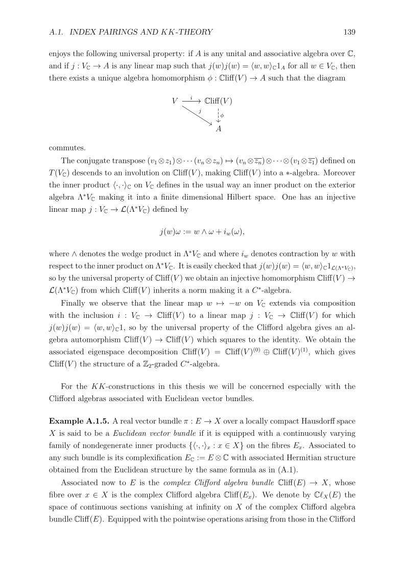
A.1. INDEX PAIRINGS AND KK-THEORY 139
enjoys the following universal property: if A is any unital and associative algebra over C,
and if j : VC → A is any linear map such that j(w)j(w) = 〈w,w〉C1A for all w ∈ VC, then
there exists a unique algebra homomorphism φ : Cliff(V )→ A such that the diagram
V Cliff(V )
A
i
jφ
commutes.
The conjugate transpose (v1⊗z1)⊗· · · (vn⊗zn) 7→ (vn⊗zn)⊗· · ·⊗(v1⊗z1) defined on
T (VC) descends to an involution on Cliff(V ), making Cliff(V ) into a ∗-algebra. Moreover
the inner product 〈·, ·〉C on VC defines in the usual way an inner product on the exterior
algebra Λ∗VC making it into a finite dimensional Hilbert space. One has an injective
linear map j : VC → L(Λ∗VC) defined by
j(w)ω := w ∧ ω + iw(ω),
where ∧ denotes the wedge product in Λ∗VC and where iw denotes contraction by w with
respect to the inner product on Λ∗VC. It is easily checked that j(w)j(w) = 〈w,w〉C1L(Λ∗VC),
so by the universal property of Cliff(V ) we obtain an injective homomorphism Cliff(V )→L(Λ∗VC) from which Cliff(V ) inherits a norm making it a C∗-algebra.
Finally we observe that the linear map w 7→ −w on VC extends via composition
with the inclusion i : VC → Cliff(V ) to a linear map j : VC → Cliff(V ) for which
j(w)j(w) = 〈w,w〉C1, so by the universal property of the Clifford algebra gives an al-
gebra automorphism Cliff(V ) → Cliff(V ) which squares to the identity. We obtain the
associated eigenspace decomposition Cliff(V ) = Cliff(V )(0) ⊕ Cliff(V )(1), which gives
Cliff(V ) the structure of a Z2-graded C∗-algebra.
For the KK-constructions in this thesis we will be concerned especially with the
Clifford algebras associated with Euclidean vector bundles.
Example A.1.5. A real vector bundle π : E → X over a locally compact Hausdorff space
X is said to be a Euclidean vector bundle if it is equipped with a continuously varying
family of nondegenerate inner products 〈·, ·〉x : x ∈ X on the fibres Ex. Associated to
any such bundle is its complexification EC := E⊗C with associated Hermitian structure
obtained from the Euclidean structure by the same formula as in (A.1).
Associated now to E is the complex Clifford algebra bundle Cliff(E) → X, whose
fibre over x ∈ X is the complex Clifford algebra Cliff(Ex). We denote by C`X(E) the
space of continuous sections vanishing at infinity on X of the complex Clifford algebra
bundle Cliff(E). Equipped with the pointwise operations arising from those in the Clifford
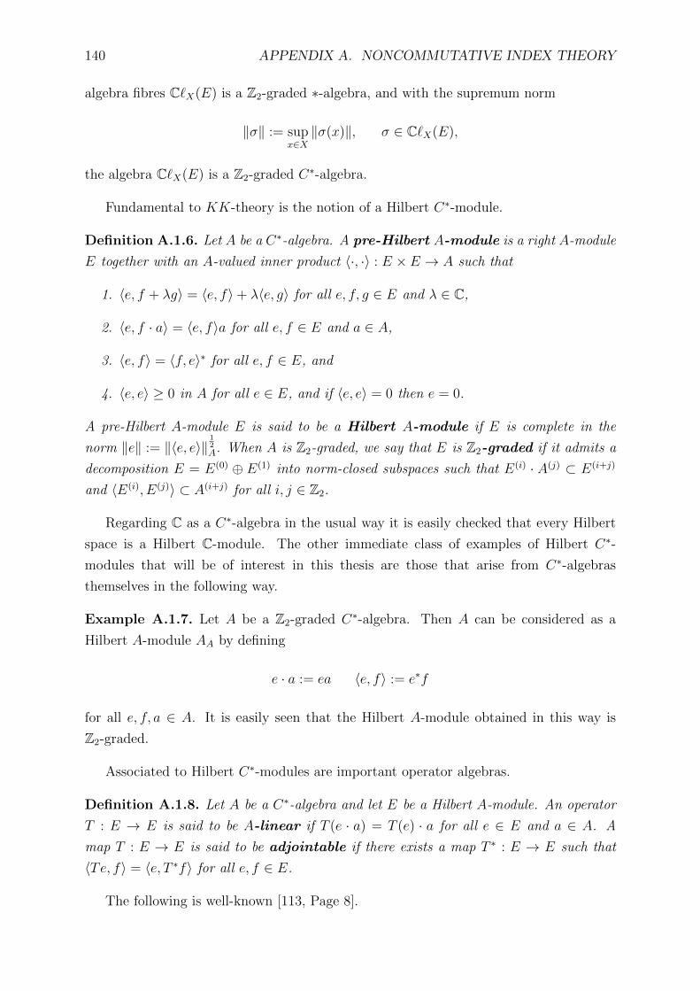
140 APPENDIX A. NONCOMMUTATIVE INDEX THEORY
algebra fibres C`X(E) is a Z2-graded ∗-algebra, and with the supremum norm
‖σ‖ := supx∈X‖σ(x)‖, σ ∈ C`X(E),
the algebra C`X(E) is a Z2-graded C∗-algebra.
Fundamental to KK-theory is the notion of a Hilbert C∗-module.
Definition A.1.6. Let A be a C∗-algebra. A pre-Hilbert A-module is a right A-module
E together with an A-valued inner product 〈·, ·〉 : E × E → A such that
1. 〈e, f + λg〉 = 〈e, f〉+ λ〈e, g〉 for all e, f, g ∈ E and λ ∈ C,
2. 〈e, f · a〉 = 〈e, f〉a for all e, f ∈ E and a ∈ A,
3. 〈e, f〉 = 〈f, e〉∗ for all e, f ∈ E, and
4. 〈e, e〉 ≥ 0 in A for all e ∈ E, and if 〈e, e〉 = 0 then e = 0.
A pre-Hilbert A-module E is said to be a Hilbert A-module if E is complete in the
norm ‖e‖ := ‖〈e, e〉‖12A. When A is Z2-graded, we say that E is Z2-graded if it admits a
decomposition E = E(0) ⊕ E(1) into norm-closed subspaces such that E(i) · A(j) ⊂ E(i+j)
and 〈E(i), E(j)〉 ⊂ A(i+j) for all i, j ∈ Z2.
Regarding C as a C∗-algebra in the usual way it is easily checked that every Hilbert
space is a Hilbert C-module. The other immediate class of examples of Hilbert C∗-
modules that will be of interest in this thesis are those that arise from C∗-algebras
themselves in the following way.
Example A.1.7. Let A be a Z2-graded C∗-algebra. Then A can be considered as a
Hilbert A-module AA by defining
e · a := ea 〈e, f〉 := e∗f
for all e, f, a ∈ A. It is easily seen that the Hilbert A-module obtained in this way is
Z2-graded.
Associated to Hilbert C∗-modules are important operator algebras.
Definition A.1.8. Let A be a C∗-algebra and let E be a Hilbert A-module. An operator
T : E → E is said to be A-linear if T (e · a) = T (e) · a for all e ∈ E and a ∈ A. A
map T : E → E is said to be adjointable if there exists a map T ∗ : E → E such that
〈Te, f〉 = 〈e, T ∗f〉 for all e, f ∈ E.
The following is well-known [113, Page 8].
A.1. INDEX PAIRINGS AND KK-THEORY 141
Proposition A.1.9. Let A be a C∗-algebra and E a Hilbert A-module. If T : E → E is
adjointable, then T and T ∗ are linear, A-linear and bounded. The collection L(E) of all
adjointable operators on E is a C∗-algebra in the operator norm.
We will in particular need the algebra of compact operators.
Definition A.1.10. Let A be a C∗-algebra and E a Hilbert A-module. The operator
θe,f ∈ L(E) defined for e, f ∈ E by the formula
θe,f (g) := e · 〈f, g〉
is said to be finite rank, and the norm closure K(E) of the algebra in L(E) generated
by all finite rank operators is a C∗-algebra called the algebra of compact operators.
We must also take into account whatever gradings may be present.
Definition A.1.11. Let A be a Z2-graded C∗-algebra and let E be a Z2-graded Hilbert
A-module. We say that T ∈ L(E) has degree j ∈ Z2 if TE(i) ⊂ E(i+j) for i ∈ Z2, and
write deg(T ) = j. This defines a grading on L(E) and K(E), making L(E) and K(E)
into Z2-graded C∗-algebras.
Finally, in order to discuss unbounded Kasparov modules, we must define the relevant
notions for unbounded operators on Hilbert modules. The best source for this is [113].
Definition A.1.12. Let A be a C∗-algebra and let E be a Hilbert A-module. Any linear,
A-linear operator D : dom(D)→ E has an adjoint D∗ defined by
dom(D∗) := e ∈ E : there exists D∗e ∈ E with 〈Dg, e〉 = 〈g, f〉 for all g ∈ dom(D)(A.2)
and D∗ : dom(D∗)→ E given by D∗(e) := D∗e. Such an operator D is said to be
1. densely defined if dom(D) is a norm-dense subspace of E,
2. closed if the graph G(D) := (e,De) : e ∈ dom(D) is norm-closed as a submodule
of E ⊕ E, and closeable if D admits a closed extension,
3. symmetric if 〈De, f〉 = 〈e,Df〉 for all e, f ∈ dom(D),
4. self-adjoint if D = D∗, and
5. regular if D is closed and densely defined, and if D∗ is densely defined such that
1 +D∗D has dense range.
The usual arguments show that any densely defined symmetric operator on a Hilbert
module E is automatically closeable. Self-adjointness and regularity, which are both nec-
essary for unbounded Kasparov modules, can be checked using the “local global principle”
for Hilbert C∗-modules which we now briefly describe, following [99].

142 APPENDIX A. NONCOMMUTATIVE INDEX THEORY
Definition A.1.13. Let A be a C∗-algebra and let E be a countably generated Hilbert
A-module. Given a state ω on A, with associated GNS Hilbert space L2(A, ω), the lo-
calisation of E by ω is the Hilbert space L2(E,ω) := E ⊗A L2(A, ω). To any linear,
A-linear operator D : dom(D) → E on E is associated its localisation Dω := D ⊗ 1 :
dom(D)⊗ L2(A, ω)→ L2(E,ω) on the localisation of E by ω.
The following extremely useful theorem is proved by Pierrot in [140, Theoreme 1.18].
The same result is given as a conjecture by Kaad and Lesch in [99, Conjecture 1.3], where
they prove a slightly weaker version [99, Theorem 1.1].
Theorem A.1.14 (Local-global principle). Let A be a C∗-algebra and let E be a countably
generated Hilbert A-module. Let D : dom(D) → E be a closed and densely defined
operator on E. Then D is self-adjoint and regular if and only if Dω is self-adjoint on the
Hilbert space L2(E,ω) for all pure states ω of A.
A.1.2 K∗, K∗ and the index pairing
K-theory is a (generalised) homology theory for C∗-algebras. We begin by briefly recalling
its definition here, following [95, Chapter 4]. All C∗-algebras we encounter in this section
are assumed separable and trivially graded.
Definition A.1.15. Let A be a unital C∗-algebra. We define K0(A) to be the abelian
group with a generator [p] for each projection p in each matrix algebra Mn(A) over A,
subject to the following relations:
1. if p and q can be joined by a continuous path of projections in Mn(A) then [p] = [q],
2. [0] = 0 for any square zero matrix, and
3. [p] + [q] = [p ⊕ q], where for p ∈ Mn(A) and q ∈ Mm(A) we denote by p ⊕ q ∈Mn+m(A) the matrix (
p 0
0 q
)
When A = C(X) is the algebra of continuous functions on a compact Hausdorff space
X, every complex vector bundle E over X determines, and is determined by, a projection
p ∈Mn(C(M)) for which p(X×Cn) = E. Thus K0(C(X)) coincides with the topological
K-theory group K0(X) defined in terms of complex vector bundles [7]. In particular,
K0(C) = K0(pt) = Z.
K-theory for unital C∗-algebras is easily seen to be covariantly functorial under C∗-
homomorphisms: that is, if φ : A → B is a homomorphism of unital C∗-algebras, we
obtain an induced homomorphism φ∗ : K0(A) → K0(B) of abelian groups sending [p]
to [φ(p)] for p ∈ Mn(A). Consequently one can define K0 for nonunital C∗-algebras as
follows.

A.1. INDEX PAIRINGS AND KK-THEORY 143
Definition A.1.16. Let A be a nonunital C∗-algebra and let A = A⊕ C be its minimal
unitization, with associated short exact sequence
0→ A→ A→ C→ 0.
We define K0(A) to be the kernel of the homomorphism K0(A) → K0(C) = Z. We
denote a generic element of K0(A) by [e] − [1e], where e ∈ Mn(A) is a projection and
where 1e ∈Mn(C) is the image of e under the projection Mn(A)→Mn(C).
Considering unitaries instead of projections we obtain K1.
Definition A.1.17. Let A be a unital C∗-algebra. We defined K1(A) to be the abelian
group with a generator [u] for each unitary u in each matrix algebra Mn(A) over A,
subject to the relations:
1. if u and v can be joined by a continuous path of unitaries in Mn(A), then [u] = [v],
2. [1] = 0 where 1 is the identity matrix in any Mn(A),
3. [u] + [v] = [u⊕ v], where we use the same notation as in Definition A.1.17.
For nonunital A we define K1(A) := K1(A).
One can define K-groups Kn of arbitrary degree using suspensions [95, Definition
4.5.4]. Bott’s periodicity theorem [95, Theorem 4.9.1] below tells us that up to isomor-
phism only K0 and K1 are of any importance.
Theorem A.1.18 (Bott’s periodicity theorem). Let A be a C∗-algebra. Then Ki(A) ∼=Ki+2(A) for all i.
It is often convenient to work with particular dense subalgebras of C∗-algebras, for
instance the algebra C∞(M) of smooth functions on a compact manifold, regarded as
a dense subalgebra of the continuous functions C(M). Such algebras of interest are
encapsulated in the following definition.
Definition A.1.19. A ∗-algebra A is said Frechet if it is equipped with a topology
induced from a countable family of seminorms in which it is complete and has jointly
continuous multiplication.
A dense ∗-subalgebra A of a C∗-algebra A is said to be stable under the holomor-
phic functional calculus if, for all a ∈ A, whenever f is a holomorphic function on
the spectrum of a for which f(0) = 0, then f(a) ∈ A.
A ∗-algebra is said to be smooth if it is both Frechet and stable under the holomorphic
functional calculus.

144 APPENDIX A. NONCOMMUTATIVE INDEX THEORY
The K-theory for smooth algebras is defined in a similar fashion to the K-theory for
C∗-algebras. In fact, as far as K-theory is concerned, smooth algebras are identical to
their enveloping C∗-algebras as follows [52, Section 3].
Proposition A.1.20. If A is a smooth subalgebra of a C∗-algebra A, then the inclusion
A → A induces an isomorphism Ki(A)→ Ki(A) for i = 0, 1.
The most interesting aspect of K-theory from the perspective of classical geometry is
the index theory of elliptic differential operators which we briefly outline now, following
[45].
Example A.1.21. If M is a compact manifold and D+ : Γ∞(E1) → Γ∞(E2) is an
elliptic, first order differential operator between smooth sections of complex Hermitian
vector bundles E1, E2 over M , then setting D− := (D+)∗ and E := E1⊕E2, the operator
D :=
(0 D−
D+ 0
): Γ∞(E)→ Γ∞(E)
extends to a bounded operator D : L21(M ;E) → L2
0(M ;E) between Sobolev spaces of
sections of E (here of course L20(M ;E) coincides with the space L2(M ;E) of square
integrable sections of E). Moreover, ellipticity of D+ guarantees that
index(D+) := dim ker(D+)− dim ker(D−)
is a finite integer. More generally, given a projection p ∈ Mn(C∞(M)) (defining a class
[p] ∈ K0(C(M))), one finds that
index(p(D+ ⊗ 1n)p) := dim ker(p(D+ ⊗ 1n)p)− dim ker(p(D− ⊗ 1n)p)
is also a finite integer. Thus D+ defines a map K0(C(M)) → Z, which is easily checked
to be a homomorphism of abelian groups.
Motivated by the index of elliptic operators as in Example A.1.21, Atiyah [8] specu-
lated that the appropriate dual homology theory to K-theory in the topological setting
ought to be built from “abstract elliptic operators”. The ideas of K-homology were de-
veloped for noncommutative C∗-algebras in [32], before finally the modern notion was
given by Kasparov [103, 104].
Definition A.1.22. Let A be a C∗-algebra. A Fredholm module over A is a triple
(π,H, F ), where H is a Hilbert space, π : A→ L(H) is a ∗-representation, and F ∈ L(H)
is such that
π(a)(1− F 2), π(a)(F − F ∗), [F, π(a)]

A.1. INDEX PAIRINGS AND KK-THEORY 145
are contained in K(H) for all a ∈ A. We say that (π,H, F ) is odd if H does not carry
a Z2-grading, and even if H carries a Z2-grading with which π(A) commutes and with
which F anticommutes.
We have the following key notions of equivalence between Fredholm modules.
Definition A.1.23. Let A be a C∗-algebra.
1. two Fredholm modules (π,H, F ) and (π′,H′, F ′) are said to be unitarily equiva-
lent if there is a unitary U : H → H′ such that (UπU∗,H′, UFU∗) = (π′,H′, F ′),
2. two Fredholm modules (π,H, F0) and (π,H, F1) are said to be homotopic if there
is a norm-continuous path t 7→ Ft, t ∈ [0, 1], such that for each t ∈ [0, 1] (π,H, Ft)is a Fredholm module.
Note that if x0 = (π,H, F ) and x1 = (π′,H′, F ′) are two even (resp. odd) Fredholm
modules over a C∗-algebra A, then their direct sum x0⊕x1 := (π⊕π′,H⊕H′, F ⊕F ′) is
also an even (resp. odd) Fredholm module. Dividing the collection of Fredholm modules
out by unitary and homotopy equivalence we obtain K-homology.
Definition A.1.24. Let A be a C∗-algebra. We define K0(A) (resp. K1(A)) to be the
abelian group with a generator [x] for each unitary equivalence class of even (resp. odd)
Fredholm modules subject to the relations:
1. if x0 and x1 are homotopic even (resp. odd) Fredholm modules, then [x0] = [x1] in
K0(A) (resp. K1(A)),
2. if x0 and x1 are even (resp. odd) Fredholm modules, then [x0] + [x1] = [x0 ⊕ x1] in
K0(A) (resp. K1(A)).
By [95, Lemma 8.3.5], any element of K0(A) (resp. K1(A)) can be represented by a
Fredholm module (π,H, F ) for which F 2 = 1 and F = F ∗. We refer to such a Fredholm
module as normalised. The final definition we need is of course that of a Fredholm
operator.
Definition A.1.25. Let H be a Hilbert space. A Fredholm operator is an element
F ∈ L(H) for which ker(F ) and ker(F ∗) are finite dimensional. The index of a Fredholm
operator F is the integer
index(F ) := dim ker(F )− dim ker(F ∗).
Finally we can define the duality between K∗ and K∗ using the index pairing as follows
[45].
146 APPENDIX A. NONCOMMUTATIVE INDEX THEORY
Proposition A.1.26. Let A be a C∗-algebra.
1. Let [p] ∈ K0(A) be represented by a projection p ∈ Mn(A), and let (π,H, F ) be
an even normalised Fredholm module. Identify A via π with a subalgebra of L(H).
If with respect to the grading H = H+⊕H− we write F =
(0 F−
F+ 0
), then
p(F+ ⊗ 1n)p : pHn → pHn is Fredholm and
〈[p], [(π,H, F )]〉 := index(p(F+ ⊗ 1n)p)
defines a pairing K0(A)⊗K0(A)→ Z.
2. Let [u] ∈ K1(A) be represented by a unitary u ∈ Mn(A), and let (π,H, F ) be an
odd normalised Fredholm module. Identify A via π with a subalgebra of L(H). Set
Pn := 12(1 +F )⊗1n acting on Hn. Then PnuPn− (1−Pn) : Hn → Hn is Fredholm,
and
〈[u], [(π,H, F )]〉 := index(PnuPn − (1− Pn))
defines a pairing K1(A)⊗K1(A)→ Z.
Example A.1.27. If M is a compact manifold, one obtains an even Fredholm module
over C(M) from a first order, elliptic differential operator D+ : Γ∞(E1) → Γ∞(E2) as
follows. As in Example A.1.21, let D− := (D+)∗ and E := E1 ⊕ E2, and define
D :=
(0 D−
D+ 0
): Γ∞(E)→ Γ∞(E).
Now by [45, Proposition 2.15], FD := D(1 + D2)−12 : L2(M ;E) → L2(M ;E) is a self-
adjoint Fredholm operator. Denoting by π the representation of C(M) on L2(M ;E) by
pointwise multiplication, the triple (π, L2(M ;E), FD) is an even Fredholm module over
C(M) defining an element in K0(C(M)). The associated index map K0(C(M)) → Zcoincides with that given in Example A.1.21.
A.1.3 KK-theory: the bounded picture
We continue in this section to assume that all algebras are separable and trivially graded.
We also assume all Hilbert modules to be countably generated. This allows us to simplify
the description of KK-theory by employing even and odd Kasparov modules.
Definition A.1.28. Let A and B be trivially graded C∗-algebras. A bounded Kasparov
A-B-module is a triple (A, πE,F ), where
1. E is a Hilbert B-module and π : A → L(E) a ∗-homomorphism of trivially graded
algebras, and
A.1. INDEX PAIRINGS AND KK-THEORY 147
2. F ∈ L(E) is such that
π(a)(1− F 2), π(a)(F − F ∗), [F, π(a)]
are contained in K(E) for all a ∈ A.
We say that a bounded Kasparov A-B-module (A, πE,F ) is even if the Hilbert module
E admits a Z2-grading, with respect to which the representation π of A is even and the
operator F is odd. Otherwise we say that (A, πE,F ) is odd.
Dividing out the collection of all unitary equivalence classes of even (resp. odd)
Kasparov A-B-modules by homotopy equivalence (see Definition B.4.1) one obtains the
groups KK0(A,B) (resp. KK1(A,B)). The group operation for Kasparov modules is
direct sum in essentially the same way as for Fredholm modules.
Crucially, KK-theory captures both the analytic K-theory and K-homology groups
associated to C∗-algebras. This relationship is easily seen to be true for K-homology,
and for the corresponding relationship with K-theory we refer to [21].
Proposition A.1.29. Let A be a C∗-algebra. Then for i = 0, 1 one has KKi(C, A) ∼=Ki(A) and KKi(A,C) ∼= Ki(A).
By far the deepest and most useful fact about KK-theory is that if A, B and D are
C∗-algebras then there is an associative product [104, Section 4, Theorem 4]
KKi(A,B)⊗KKj(B,D)→ KKi+j(A,D)
called the Kasparov product. In particular, taking A = D = C recovers the index pairing
between K-theory and K-homology. In general, the Kasparov product with an element
x ∈ KKi(B,D) defines a homomorphism
· ⊗B x : K∗(A)→ K∗+i(D)
of K-theory groups. Kasparov modules and the Kasparov product therefore puts index
theory, thought of as “index maps between K-theory groups”, on a systematic and in-
credibly general footing. Unfortunately, the Kasparov product as given in [104, 105] is
non-constructive. The situation in the bounded setting is improved using the technol-
ogy of connections developed by Connes and Skandalis [61, Appendix A], which we will
employ when discussing groupoid equivariant KK-theory in Appendix B.
A.1.4 KK-theory: the unbounded picture and spectral triples
The wish to be able to compute Kasparov products at the level of representative Kasparov
modules provided motivation for the development of an equivalent, but more computa-

148 APPENDIX A. NONCOMMUTATIVE INDEX THEORY
tionally tractible and geometrically meaningful picture of KK-theory, whose building
blocks are unbounded Kasparov modules. We continue to assume all C∗-algebras to be
separable and trivially graded and all Hilbert modules to be countably generated.
Definition A.1.30. Let A and B be C∗-algebras. An unbounded Kasparov A-B-
module is a triple (A, πE,D), where
1. E is a Hilbert B-module, and π : A→ L(E) a ∗-homomorphism,
2. A ⊂ A is a dense ∗-subalgebra of A, and
3. D : dom(D)→ E is a densely-defined, unbounded, self-adjoint and regular operator
on E such that [D, π(a)] ∈ L(E) and such that π(a)(1 + D2)−12 ∈ K(E) for all
a ∈ A.
We say that an unbounded Kasparov A-B-module (A, πE,D) is even if the Hilbert module
E admits a Z2-grading for which the representation π of A is even, and for which the
operator D is odd. Otherwise we say that (A, πE,D) is odd.
As shown in [13], given any unbounded Kasparov A-B-module (A, πE,D), one obtains
a bounded Kasparov A-B-module (A, πE,FD = D(1 + D2)−12 ) and hence a class in
KK(A,B). The use of unbounded representatives of KK classes has proved quite fruitful
in the search for a constructive procedure to compute Kasparov products (see for instance
[111, 117, 121, 100, 31, 122]), but such a procedure in complete generality at this stage
still remains elusive.
Unbounded Kasparov modules are typically more geometrically fundamental objects
than their bounded counterparts. This fact is best illustrated with another example.
Example A.1.31. Let M be a compact manifold, equipped with a Z2-graded vector
bundle E and a first order, elliptic differential operator D : Γ∞(E) → Γ∞(E) as in Ex-
amples A.1.21 and A.1.27. Then (C∞(M), L2(M ;E), D) is an even unbounded Kasparov
C(M)-C-module. The associated bounded transform (C(M), L2(M ;E), D(1 +D2)−12 ) is
the Fredholm module encountered in Example A.1.27.
Note that the operator D is by far a more geometrically natural object than is FD =
D(1 + D2)−12 . Indeed, while D is a local operator in the sense that its action at a point
can be computed simply by calculating some derivatives in a neighbourhood of that point,
the action of the (pseudodifferential) operator FD at a point must be computed via an
integral of a complicated function over all of M , and is therefore inherently non-local.
This makes FD a much clumsier object to use in computations.
An unbounded Kasparov A-C-module (A, πH, D) is a spectral triple for A in the
sense of Connes-Moscovici [59]. As we know, the Kasparov product with (A,H, D)

A.1. INDEX PAIRINGS AND KK-THEORY 149
defines a homomorphism K∗(A) → Z, but it is instructive at this point to factorise
this homomorphism as the composition
K∗(A)→ K0(K(H))Tr−→ Z,
where Tr : K0(K(H))→ Z is the isomorphism induced by sending a compact projection
p on H to the integer Tr(p), where Tr is the usual trace on B(H). With this factorisation
in mind, one is naturally led to the question of what sort of structure arises if one were
to replace K(H) with some other algebra, and Tr with some other trace.
Definition A.1.32. Let N be a von Neumann algebra, with set of positive elements
(those of the form a∗a) denoted by N+. A trace τ : N+ → [0,∞] on N is said to be
1. faithful if τ(x) = 0 implies x = 0 in N+,
2. normal if whenever x ∈ N+ is the limit of an increasing net (xλ)λ∈Λ ⊂ N+ one
has τ(x) = supλ τ(xλ), and
3. semifinite if dom(τ) := x ∈ N : τ(x∗x) <∞ is weakly dense in N .
If N is associated with a faithful, normal, semifinite trace τ : N+ → [0,∞] then we refer
to the pair (N , τ) as a semifinite von Neumann algebra. If (N , τ) is a semifinite
von Neumann algebra, we denote by Kτ (N ) the norm-closed ideal in N generated by
τ -finite projections, and refer to Kτ (N ) as the ideal of τ-compact operators [72].
Example A.1.33. We will encounter two examples of semifinite von Neumann algebras
in this thesis.
1. The pair (L(H),Tr) is a semifinite von Neumann algebra for any separable Hilbert
space H.
2. Suppose B is a C∗-algebra equipped with a faithful, norm-lower-semicontinuous,
semifinite trace. Then if E is a Hilbert B-module, with B-valued inner product
denoted 〈·, ·〉, we form the GNS Hilbert space L2(E, τ) from the inner product
(e|f) := τ(〈e, f〉) defined on E. Then by the results in [112] we obtain a faithful,
normal, semifinite trace Trτ on the von Neumann algebra obtained as the weak
closure N := L(E)′′ ⊂ L(L2(E, τ)) of the adjointable operators on E acting on
L2(E, τ). The trace Trτ satisfies
Trτ (θe,f ) := τ(〈e, f〉)
for all e, f ∈ E, where θe,f is the compact operator on E corresponding to e, f .
We also need a notion of compatibility between unbounded operators and von Neu-
mann algebras.

150 APPENDIX A. NONCOMMUTATIVE INDEX THEORY
Definition A.1.34. Let N ⊂ L(H) be a von Neumann algebra on a Hilbert space H.
We say that a closed and densely defined unbounded operator D : dom(D)→ H on H is
affiliated to N if every unitary U in the commutant of N commutes with D.
Definition A.1.35. Let (N , τ) be a semifinite von Neumann algebra, regarded as an
algebra of operators on a Hilbert space H. A semifinite spectral triple relative to
(N , τ) is a triple (A, πH, D) consisting of a ∗-algebra A represented in N by π : A →N ⊂ B(H), and a densely defined, unbounded, self-adjoint operator D affiliated to Nsuch that
1. π(a) dom(D) ⊂ dom(D) so that [D, π(a)] is densely defined, and moreover extends
to a bounded operator on H for all a ∈ A,
2. π(a)(1 +D2)−12 ∈ Kτ (N ) for all a ∈ A.
We say that (A, πH, D) is even if A is even and D is odd for some Z2-grading on H,
and otherwise we call (A, πH, D) odd.
Just as ordinary spectral triples in the sense of Connes-Moscovici are really unbounded
Kasparov modules, semifinite spectral triples also have a close relationship with KK-
theory.
Proposition A.1.36. Let A ⊂ A smooth subalgebra of a C∗-algebra A.
1. [101, Theorem 5.3] Let (N , τ) be a semifinite von Neumann algebra, and suppose
that (A, πH, D) is an odd (resp. even) semifinite spectral triple relative to (N , τ).
Let FD := D(1 +D2)−12 be the bounded transform of D, and let BD be the separable
C∗-subalgebra of N generated by the elements
FD[FD, a], b[FD, a], FDb[FD, a], aϕ(D)
for all a, b ∈ A and ϕ ∈ C0(R). Then the triple (A,mBD, D) is an odd (resp. even)
unbounded Kasparov A-BD-module. Here m is the representation of A on BD by
multiplication on the countably generated Hilbert BD-module BD, and the operator
D affiliated to N acts as an unbounded multiplier on BD.
2. [118, Proposition 2.13] Conversely, suppose that (A, πE,D) is an odd (resp. even)
unbounded Kasparov A-B-module, and that τ is a faithful, semifinite, norm-lower-
semicontinuous trace on B. Then (with a slight abuse of notation)
(A, π ⊗ 1E ⊗B L2(B, τ), D ⊗ 1) = (A, πL2(E, τ), D)
is an odd (resp. even) semifinite spectral triple relative to the semifinite von Neu-
mann algebra (L(E)′′,Trτ ) considered in Example A.1.33.

A.2. CYCLIC COHOMOLOGY AND INDEX FORMULAE 151
In light of Proposition A.1.36, we see that any odd (resp. even) semifinite spec-
tral triple (A, πH, D) relative to a semifinite von Neumann algebra (N , τ) has a well-
defined, real-valued pairing with K1(A) (resp. K0(A)), where A is the norm completion
of A. Specifically, the Kasparov product with the associated unbounded Kasparov A-
BD-module (A,mBD, D) defines a homomorphism
· ⊗A [D] : K∗(A)→ K0(BD)
(with ∗ = 0 for (A, πH, D) even and ∗ = 1 for (A, πH, D) odd), while the trace τ :
Kτ (N )+ → R induces a map τ∗ : K0(BD) → R. Thus one obtains a pairing with K∗(A)
defined by
〈x, [(A, πH, D)]〉 := τ∗(x⊗A [D]) ∈ R
for x ∈ K∗(A) of appropriate parity. In the next section we will give a formula, due to
A. Carey, V. Gayral, A. Rennie and F. Sukochev (following Connes-Moscovici [59] and
Higson [94]) for computing this numerical index pairing.
A.2 Cyclic cohomology and index formulae
The Atiyah-Singer index theorem [10, 11, 12] says that if D is an elliptic differential
operator on a Z2-graded vector bundle over a compact manifold M then its index can
be computed by a de Rham cohomological formula. As in Example A.1.31, one knows
that such an operator defines an even, unbounded Kasparov C(M)-C-module (that is, a
spectral triple). So the Atiyah-Singer index theorem can be viewed as a de Rham-type
formula for the pairing of a spectral triple over a commutative algebra with K-theory.
The starting point for the local index formula in noncommutative geometry is in
asking whether the Atiyah-Singer index formula can be extended to noncommutative
algebras. Connes [54] recognised that such a task requires a noncommutative version of
de Rham cohomology, and introduced cyclic cohomology as its replacement. By doing so,
Connes [54] was able to give a formula for the index pairing of Fredholm modules with
K-theory over noncommutative algebras, providing the first generalisation of the Atiyah-
Singer index formula to the noncommutative setting. This initial attempt, however,
suffered from the same lack of computability inherent in using the bounded transform
D(1+D2)−12 of geometric operators D that is required in constructing Fredholm modules
from geometric data, as in Example A.1.31.
A decade later, Connes and Moscovici [59] introduced the local index formula for
spectral triples, putting noncommutative index calculations on a more computationally
tractible footing. Their work has since been expanded upon and generalised in a number
of directions, in particular to formulae for the index pairings obtained from nonunital,
semifinite spectral tiples [15, 39, 40, 41, 42, 36, 37]. In this section we briefly cover the
152 APPENDIX A. NONCOMMUTATIVE INDEX THEORY
basics of cyclic cohomology and give the local index formula for semifinite spectral triples,
which will be crucial in establishing an index theorem for the Godbillon-Vey invariant of
codimension 1 foliations. Details for all that will be presented can be found in [116, 56]
and [37].
A.2.1 Cyclic cohomology
The easiest route to cyclic cohomology is via Connes’ λ-complex. For any associative
algebra A over C, we define Cnλ (A) to be the space of (n + 1)-linear functionals ϕ on A
for which
ϕ(a1, . . . , an, a0) = (−1)nϕ(a0, . . . , an)
for all a0, . . . , an ∈ A. The Hochschild coboundary operator restricts to an operator
b : Cnλ (A)→ Cn+1
λ (A) defined by
(bϕ)(a0, . . . , an+1) :=n∑j=1
(−1)jϕ(a0, . . . , ajaj+1, . . . , an) + (−1)n+1ϕ(an+1a0, . . . , an)
(A.3)
for a0, . . . , an+1 ∈ A. It is easily verified that b2 = 0, and so the cyclic cohomology of Acan be defined as follows.
Definition A.2.1. The cyclic cohomology HC∗(A) of A is defined to be the cohomology
of the cochain complex (C∗λ(A), b).
While Connes’ λ-complex is sufficient for many purposes, the local index formula for
semifinite spectral triples requires the (b, B)-bicomplex picture of cyclic cohomology. For
this we will for the time being require A to be unital with unit 1A.
We denote by Cn(A) the space of n+ 1-linear functionals ϕ on A such that
ϕ(a0, . . . , an) = 0
whenever any one of the ai ∈ A, i ≥ 1, is equal to 1A. We then consider the bicomplex
B∗(A) given by
......
...
C2(A) C1(A) C0(A)
C1(A) C0(A)
C0(A)
b
B
b
B
b
b
B
b
b

A.2. CYCLIC COHOMOLOGY AND INDEX FORMULAE 153
where b is defined as in (A.3), and where the operator B : Cn(A)→ Cn−1(A) is defined
for all n ≥ 1 by the formula
(Bϕ)(a0, . . . , an−1) :=n−1∑j=1
(−1)(n−1)jϕ(1A, ai, ai+1, . . . , an−1, a0, . . . , ai−1)
for a0, . . . , an−1 ∈ A. It is again easily verified that B2 = 0 and that bB + Bb = 0. We
obtain the associated total complex TotB(A) defined by
Tot2n B(A) :=n⊕j=0
C2j(A) Tot2n+1 B(A) :=n⊕j=0
C2j+1(A)
with coboundary map b + B. By the cohomological version of the result [116, Corollary
2.1.10], we obtain the following alternative characterisation of cyclic cohomology for unital
algebras.
Proposition A.2.2. For unital A, the cohomology of the total complex (Tot∗ B(A), b+B)
coincides with the cyclic cohomology HC∗(A).
Now if A is nonunital, the inclusion C → A⊕C is injective and so we obtain the
exact sequence
0→ C → A⊕C→ A→ 0
of vector spaces. Therefore the induced map B(A⊕C)→ B(C) of double complexes is a
surjection, and we define B(A) to be its kernel, giving an exact sequence
0→ B(A)→ B(A⊕C)→ B(C)→ 0
of double complexes. From the cohomological form of [116, Proposition 2.2.14] we then
obtain the (b, B) characterisation of cyclic cohomology for nonunital algebras.
Proposition A.2.3. The cohomology of the total complex (Tot∗ B(A), b + B) coincides
with the cyclic cohomology HC∗(A).
It is the (b, B) picture, for not necessarily unital algebras, that will be used as the
receptacle for the local index formula for semifinite spectral triples.
A.2.2 The local index formula
Before we can give the local index formula for semifinite spectral triples we need to define
some smoothness and summability notions for semifinite spectral triples. Summability
itself is relatively easy to define.
154 APPENDIX A. NONCOMMUTATIVE INDEX THEORY
Definition A.2.4. Let (A,H, D) be a semifinite spectral triple relative to a semifinite
von Neumann algebra (N , τ) on H. We say that (A,H, D) is finitely summable if
there exists real s > 0 such that τ(|a(1 + D2)−s2 |) <∞ for all a ∈ A. In such a case we
define
p := infs > 0 : τ(|a|(1 +D2)−s2 ) for all a ∈ A
and refer to p as the spectral dimension of (A,H, D).
Smoothness and its relationship with summability is somewhat complicated for spec-
tral triples over nonunital algebras. Throughout, we let D be a self-adjoint, densely
defined operator affiliated to a semifinite von Neumann algebra (N , τ) on a Hilbert space
H, and we let p ≥ 1 be an integer. We think of D as encoding a “noncommutative volume
element” (1 + D2)−12 in N , therefore defining notions of integrability (summability) as
follows.
Definition A.2.5. For real s > 0, define a weight ϕs on N by
ϕs(T ) := τ((1 +D2)−
s4T (1 +D2)−
s4
)∈ [0,∞]
for all T ∈ N+.
It can be proved [37, Lemma 1.2], the ϕs are faithful, normal, semifinite weights, and
we define the weight domains
dom(ϕs)+ := T ∈ N+ : ϕs(T ) <∞
and
dom(ϕs)12 := T ∈ N : T ∗T ∈ dom(ϕs)+.
Now since dom(ϕs)12 is not generally closed under involution we make the following defi-
nition.
Definition A.2.6. We define the ∗-algebra
B2(D, p) :=⋂s>p
(dom(ϕs)
12 ∩(
dom(ϕs)12
)∗).
For n ∈ N, we obtain norms
Qn(T ) :=(‖T‖2 + ϕp+1/n(|T |2) + ϕp+1/n(|T ∗|2)
)which take finite values on B2(D, p) and define a topology on B2(D, p) that is stronger
than the norm topology.

A.2. CYCLIC COHOMOLOGY AND INDEX FORMULAE 155
Equipped with the topology arising from the norms Qn(T ), B2(D, p) ⊂ N is a smooth
algbebra [37, Proposition 1.6, Lemma 1.8], which we think of as being the algebra of
operators in N that are “square integrable” with respect to the “volume element” defined
by D. To obtain the integrable operators in N , we define B2(D, p)2 to be the finite span
of products from B2(D, p), and define a functional Pn thereon by
Pn(T ) := inf
k∑i=1
Qn(Ti,1)Qn(Ti,2) : T =k∑i=1
Ti,1Ti,2, Ti,1Ti,2 ∈ B2(D, p)
,
where the infimum is taken over all such possible representations of T . The Pn are norms
on B2(D, p)2, arising from the projective tensor product topology on B2(D, p)⊗B2(D, p)
[37].
Definition A.2.7. We define B1(D, p) to be the completion of B2(D, p)2 with respect to
the Frechet topology induced by the norms Pn.
By [37, Corollary 1.12, Proposition 1.18], B1(D, p) is a smooth ∗-subalgebra of N ,
which we think of as the algebra of operators in N that are integrable with respect to D.
Having defined the algebra of integrable operators, we can define what it means for the
derivatives of operators (with respect to D) to be integrable.
Definition A.2.8. Let H∞ :=⋂k≥0 dom(Dk). For an operator T ∈ N such that T :
H∞ → H∞, we set
δ(T ) := [|D|, T ].
For integer k ≥ 0, we define
Bk1(D, p) := T ∈ N : for all l = 0, . . . , k, δl(T ) ∈ B1(D, p)
and
B∞1 (D, p) :=∞⋂k=0
Bk1(D, p).
The ∗-subalgebras Bk1(D, p), k ∈ N∪∞ of N can be equipped with topologies [37,
Proposition 1.22, Lemma 1.29]. Regarding δ as the “derivative with respect to |D|”, the
algebras Bk1(D, p) are to be thought of as the algebras of operators in N that are k-times
differentiable with respect to |D| and for which all derivatives up to order k are integrable.
Having such algebras in hand we can now give the definition of smooth summability for
spectral triples.
Definition A.2.9. Let (A,H, D) be a semifinite spectral triple relative to (N , τ). We say
that (A,H, D) is smoothly summable if it is finitely summable of spectral dimension
some integer p > 1, and if A∪[D,A] ⊂ B∞1 (D, p).

156 APPENDIX A. NONCOMMUTATIVE INDEX THEORY
The following sufficient condition for smooth summability of a spectral triple is simple
to check and is used in the index theorem for the Godbillon-Vey semifinite spectral triple.
Proposition A.2.10. [37, Proposition 2.21] Let (A,H, D) be a finitely summable semifi-
nite spectral triple of spectral dimension p relative to (N , τ), and for T ∈ L(H) set
L(T ) = (1 +D2)−12 [D2, T ]. If for all T ∈ A∪[D,A], integers k ≥ 0 and s > p we have
τ(∣∣(1 +D2)−
s4Lk(T )(1 +D2)−
s4
∣∣) <∞,then (A,H, D) is smoothly summable.
Finally, in order to simplify the local index theorem maximally, we require the follow-
ing property of our spectral triples.
Definition A.2.11. Let (A,H, D) be a smoothly summable, semifinite spectral triple of
spectral dimension p relative to (N , τ). For a ∈ A, we use the notation da := [D, a],
define da(0) := da, and inductively define da(n) := [D2, da(n−1)] for integer n ≥ 1. We say
that the spectral dimension is isolated if for any element b ∈ N of the form
b = a0da(k1)1 · · · da(km)
m (1 +D2)−|k|−m/2, a0, . . . , am ∈ A,
with k = (k1, . . . , km) ∈ (N∪0)m a multi-index and |k| = k1 +· · ·+km, the zeta function
ζb(z) := τ(b(1 +D2)−z)
has an analytic continuation to a deleted neighbourhood of z = 0. This being the case, we
define the numbers
τj(b) := resz=0 zjζb(z)
for all integer j ≥ −1.
Finally we can give the residue cocycle. For a multi-index k ∈ (N∪0)m, we define
the number
α(k)−1 := k1! · · · km!(k1 + 1)(k1 + k2 + 2) · · · (|k|+m).
For integers n ≥ 1 and l ≥ 0, we also define the non-negative rational numbers σn,l and
σn,l by the identities
n−1∏j=0
(z + j) =n∑j=1
zjσn,j,
n−1∏j=0
(z + j + 1/2) =n∑j=0
zjσn,j.
Definition A.2.12. Suppose that (A,H, D) is a smoothly summable, semifinite spectral
triple with isolated spectral dimension p relative to (N , τ). Given a0, . . . , am ∈ A, the
residue cocycle (φm)Mm=0 is defined as follows:
A.2. CYCLIC COHOMOLOGY AND INDEX FORMULAE 157
If (A,H, D) is even, with grading γ on H,
φ0(a0) := τ−1(a0),
and, setting |k|+m/2,
φm(a0, . . . , am) :=M−m∑|k|=0
(−1)|k|α(k)h∑j=1
σh,jτj−1
(γa0da
(k1)1 · · · da(km)
m (1 +D2)−|k|−m/2)
for m even, and with φm = 0 for m odd.
If (A,H, D) is odd, setting h = |k|+ (m− 1)/2,
φm(a0, . . . , am) :=√
2πiM−m∑|k|=0
(−1)|k|α(k)h∑j=0
σh,jτj
(a0da
(k1)1 · · · da(km)
m (1 +D2)−|k|−m/2)
for m odd, and with φm = 0 for m even.
The residue cocycle of a smoothly summable, semifinite spectral triple (A,H, D) with
isolated spectral dimension is a (b, B)-cocycle for A [37, Proposition 3.19, Proposition
3.20]. Ultimately one wishes to feed a representative x of a class [x] in K∗(A) into the
residue cocycle to compute the index pairing 〈[x], [(A,H, D)]〉. Observe, however, that
the residue cocycle only accepts elements of A, so we need to be careful in ensuring that
A is large enough that any class in K∗(A) can be represented by an element of A. By
[37, Proposition 2.20], smoothness and summability of (A,H, D) guarantees that A can
be completed to a smooth algebra Aδ,ϕ for which (Aδ,ϕ,H, D) is a smoothly summable,
semifinite spectral triple, and then by Proposition A.1.20 one can always choose repre-
sentatives for K∗(A) from the smooth algebra Aδ,ϕ.
That the residue cocycle computes the index pairing with K-theory is encapsulated
in the following result [37, Theorem 3.33 (3)].
Theorem A.2.13. Let (A,H, D) be a smoothly summable, semifinite spectral triple with
isolated spectral dimension p.
If (A,H, D) is even and [e]− [1e] ∈ K0(A) is represented by a projection e ∈Mn(A),
then setting M to be the largest even integer less than or equal to p+ 1 we have
〈[e]− [1e], [(A,H, D)]〉 = φ0(e− 1e) +M∑k=1
φ2k
((−1)k
(2k)!
k(e− 1/2)⊗ e⊗ · · · ⊗ e︸ ︷︷ ︸
2k times
)
),
where (φm)Mm=0 is the residue cocycle for the spectral triple (Mn(A),Hn, D ⊗ 1n).
If (A,H, D) is odd and [u] ∈ K1(A) is represented by a unitary u ∈ Mn(A), then
158 APPENDIX A. NONCOMMUTATIVE INDEX THEORY
setting M to be the largest odd integer less than or equal to p+ 1 we have
〈[u], [(A,H, D)]〉 = − 1√2πi
M∑k=0
φ2k+1
((−1)kk! (u∗ ⊗ u)⊗ · · · ⊗ (u∗ ⊗ u)︸ ︷︷ ︸
k+1 times
),
where (φm)Mm=0 is the residue cocycle for the spectral triple (Mn(A),Hn, D ⊗ 1n).

Appendix B
Groupoids and equivariant
KK-theory
Groupoid-equivariant KK-theory has been treated in [115]. Essentially, for a groupoid Gwith unit space G(0), a G-algebra A can be regarded as (sections of) a bundle of algebras
A → G(0) (a so-called C0(G(0))-algebra), with isomorphisms indexed by the elements of
the groupoid mapping fibres between each other in a way which is compatible with the
groupoid multiplication and topology. A particularly convenient way to characterise such
an object is to “pull back” the bundle A→ G(0) to G via the range and source maps, and
insist on an isomorphism between these pullbacks. When G is Hausdorff, this may be
achieved on an algebraic level using balanced tensor products with the C∗-algebra C0(G).
Of course, when G is a non-Hausdorff topological space we are not guaranteed a wealth
of interesting continuous functions on G, so while C0(G) is still a C∗-algebra and the
balanced tensor products make sense, they may carry very little interesting topological
information. Since holonomy groupoids are generally locally Hausdorff only, the method
used in [115] to build a groupoid-equivariant KK-theory requires extension to the locally
Hausdorff case.
In [134], Paul Muhly and Dana Williams exploit the locally Hausdorff structure of
such groupoids in order to define meaningful notions of groupoid actions on algebras.
Their approach reduces in the Hausdorff case to the setting explored in [115]. Using
these ideas, it is possible to recover the algebraic formulation of groupoid-equivariant
KK-theory found in [115] using balanced tensor products in a way that generalises to
locally Hausdorff groupoids. In keeping with [115], the KK-material will be developed
from the algebraic point of view of balanced tensor products. Since all examples we will
be considering for foliation theory are more naturally bundle-theoretic in nature, however,
we will present both the algebraic and bundle-theoretic points of view of algebras and
modules. We will also give the result of Muhly and Williams that shows these two points
of view are entirely equivalent.
159

160 APPENDIX B. GROUPOIDS AND EQUIVARIANT KK-THEORY
Much of the material appearing in this appendix is due to Muhly and Williams ([134],
[152]), and to Le Gall ([115]). There are nonetheless many gaps to be filled, and we give
detailed proofs wherever the existing literature is insufficient.
B.1 Groupoids
Groupoids simultaneously generalise both spaces and groups, and can therefore encode
complicated dynamical information. In this section we will define what is meant by a
locally compact, locally Hausdorff topological groupoid.
Definition B.1.1. A groupoid (G(0),G, r, s,m, i) consists of a set G, the total space,
with a distinguished subset G(0), the unit space, maps r, s : G → G(0) called the range
and source respectively, a multiplication map m : G ×s,r G → G and an inversion
map i : G → G such that
1. i satisfies i2 = id,
2. m is associative,
3. r i = s.
4. m(u, x) = u = m(y, u) for all u ∈ G with r(u) = y and s(u) = x.
We will usually denote a groupoid (G(0),G, r, s,m, i) by simply G, m(u, v) by simply
uv, and i(u) by u−1.
Definition B.1.2. Let G be a groupoid. We say that G is a topological groupoid if Gis a topological space and if r, s,m, i are all continuous maps, with r, s furthermore being
required to be open.
In this thesis, we will always assume topological groupoids to be equipped with locally
compact, locally Hausdorff, second-countable topologies for which the unit space is a locally
compact, Hausdorff subspace.
We will need the definition of a G-action on a space X. Since one of the most obvious
examples of a groupoid action on a topological space is given by the action of G on itself,
we will need to permit actions on locally Hausdorff spaces.
Definition B.1.3. Let X be a locally compact, locally Hausdorff space. A left action
of G on X consists of a continuous map p : X → G(0) called the anchor map, together
with a continuous map G ×s,pX → X, denoted (u, x) 7→ u · x, such that
1. p(u · x) = r(u) for all (u, x) ∈ G ×s,pX,
2. (uv) · x = u · (v · x) for all (v, x) ∈ G ×s,pX and (u, v) ∈ G(2),
B.2. UPPER-SEMICONTINUOUS BUNDLES 161
3. p(x) · x = x for all x ∈ X.
One can define a right action in an analogous way on the set X ×p,r G, and can be
obtained from a left action by defining (x ·u) := u−1 ·x for all (x, u) ∈ X×p,r G. In either
case, we say that G acts on X and that X is a G-space.
If G acts on a space X, then the sets GnX := G ×s,pX and X o G := X ×p,r G both
admit the structure of topological groupoids with unit space X, and are isomorphic as
topological groupoids under the map X×p,r G 3 (x, u) 7→ (u, u−1 ·x) ∈ G ×s,pX. We refer
to both of these groupoids as the action groupoid corresponding to the action of G on X.
B.2 Upper-semicontinuous bundles
We give a study of upper-semicontinuous bundles of spaces, algebras and modules. Vir-
tually all of this material comes from [152] (see also [73]), with slight additions made
explicitly where needed. Concerning notation, for any map f : Y → X of sets, we will
for each x ∈ X denote by Yx the fibre f−1x over x.
Definition B.2.1. Suppose that X is a locally compact Hausdorff space. By an upper-
semicontinuous Banach-bundle over X, we mean a topological space A together with
an open surjective map pA : A→ X and a complex Banach space structure on each fibre
Ax such that
1. the map a 7→ ‖a‖ is upper semicontinuous from A to R (that is, for all ε > 0,
a ∈ A : ‖a‖ ≥ ε is closed),
2. the map + : A×pA,pA A→ A given by (a, b) 7→ a+ b is continuous,
3. the map C× A→ A given by (λ, a) 7→ λa is continuous,
4. if ai is a net in A such that pA(ai)→ x and ‖ai‖ → 0, then ai → 0x, where 0x is
the zero element in Ax.
A section of pA is a function β : X → A such that pAβ = idX . The space of continuous
sections of pA is denoted Γ(X;A) and the space of continuous sections vanishing at infinity
in the norm topology on the fibres is denoted Γ0(X;A).
We remark that requiring Hausdorff separability of X in the above definition is nec-
essary to guarantee that there are “enough sections” of a given bundle. Specifically, it
can be shown [134] that when X is locally compact and Hausdorff, for each x ∈ X and
a ∈ Ax, we are guaranteed a continuous section β such that β(x) = a. We cannot hope
for such an abundance of continuous sections when X is not Hausdorff.
Of great importance for the theory is the pullback of an upper-semicontinuous Banach-
bundle by a continuous map.
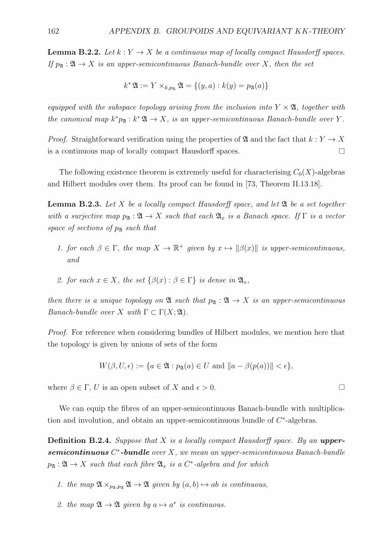
162 APPENDIX B. GROUPOIDS AND EQUIVARIANT KK-THEORY
Lemma B.2.2. Let k : Y → X be a continuous map of locally compact Hausdorff spaces.
If pA : A→ X is an upper-semicontinuous Banach-bundle over X, then the set
k∗A := Y ×k,pA A = (y, a) : k(y) = pA(a)
equipped with the subspace topology arising from the inclusion into Y × A, together with
the canonical map k∗pA : k∗A→ X, is an upper-semicontinuous Banach-bundle over Y .
Proof. Straightforward verification using the properties of A and the fact that k : Y → X
is a continuous map of locally compact Hausdorff spaces.
The following existence theorem is extremely useful for characterising C0(X)-algebras
and Hilbert modules over them. Its proof can be found in [73, Theorem II.13.18].
Lemma B.2.3. Let X be a locally compact Hausdorff space, and let A be a set together
with a surjective map pA : A→ X such that each Ax is a Banach space. If Γ is a vector
space of sections of pA such that
1. for each β ∈ Γ, the map X → R+ given by x 7→ ‖β(x)‖ is upper-semicontinuous,
and
2. for each x ∈ X, the set β(x) : β ∈ Γ is dense in Ax,
then there is a unique topology on A such that pA : A → X is an upper-semicontinuous
Banach-bundle over X with Γ ⊂ Γ(X;A).
Proof. For reference when considering bundles of Hilbert modules, we mention here that
the topology is given by unions of sets of the form
W (β, U, ε) := a ∈ A : pA(a) ∈ U and ‖a− β(p(a))‖ < ε,
where β ∈ Γ, U is an open subset of X and ε > 0.
We can equip the fibres of an upper-semicontinuous Banach-bundle with multiplica-
tion and involution, and obtain an upper-semicontinuous bundle of C∗-algebras.
Definition B.2.4. Suppose that X is a locally compact Hausdorff space. By an upper-
semicontinuous C∗-bundle over X, we mean an upper-semicontinuous Banach-bundle
pA : A→ X such that each fibre Ax is a C∗-algebra and for which
1. the map A×pA,pA A→ A given by (a, b) 7→ ab is continuous,
2. the map A→ A given by a 7→ a∗ is continuous.

B.2. UPPER-SEMICONTINUOUS BUNDLES 163
It is clear that for any upper-semicontinuous C∗-bundle pA : A → X, one can equip
Γ0(X;A) with the structure of a C∗-algebra using the sup-norm and pointwise operations.
Moreover, it admits a C0(X)-module structure defined by
(f · ρ)(x) := f(x)ρ(x), x ∈ X
for f ∈ C0(X) and ρ ∈ Γ0(X;A). Algebras which admit such a structure are called
C0(X)-algebras.
Definition B.2.5. Let X be a locally compact Hausdorff space. A C∗-algebra A is said to
be a C0(X)-algebra if it admits a nondegenerate homomorphism C0(X)→ ZM(A) into
the center of the multiplier algebra of A. A homomorphism φ : A→ B of C0(X)-algebras
A and B is said to be a C0(X)-homomorphism if it is simultaneously a C0(X)-module
homomorphism, that is φ(f · a) = f · φ(a) for all f ∈ C0(X) and a ∈ A.
Example B.2.6. The primary example that is of interest in this thesis is when we have a
continuous surjection π : Y → X of locally compact Hausdorff spaces Y and X. In such a
case, C0(Y ) is a C0(X)-algebra: every f ∈ C0(X) induces a multiplier of C0(Y ) obtained
by defining f · g(y) := f(π(y))g(y) for all y ∈ Y . Note that C0(Y ) can be regarded as a
bundle of C∗-algebras over X, whose fibre over x ∈ X is C0(Yx), where Yx = π−1x is
the fibre of Y over X.
Using Lemma B.2.3, we can show that every C0(X) algebra is isomorphic to Γ0(X;A)
for some upper-semicontinuous C∗-bundle pA : A→ X.
Proposition B.2.7. Let X be a locally compact Hausdorff space and let A be a C0(X)-
algebra. There exists an upper-semicontinuous C∗-bundle pA : A → X such that A is
C0(X)-isomorphic to Γ0(X;A). If A = Γ0(X;A) and B = Γ0(X;B) are C0(X)-algebras,
any C0(X)-homomorphism φ : A → B induces a continuous bundle map ϕ : A → B
whose restriction to each fibre is a C∗-homomorphism, and vice versa.
Proof. For each x ∈ X, one sets Ax := A/(Ix ·A), where Ix is the kernel of the evaluation
functional f 7→ f(x) on C0(X). Defining A :=⊔x∈X Ax and Γ := x 7→ a : a ∈ Ax, the
first part of the result follows from Lemma B.2.3 and some continuity arguments on the
multiplication and involution [152, Theorem C.25].
Now suppose that φ : A→ B is a C0(X)-homomorphism between two C0(X)-algebras
A = Γ0(X;A) and B = Γ0(X;B). Using the fact that upper-semicontinuous bundles
over the locally compact Hausdorff space X admit “enough sections”, the corresponding
bundle map ϕ : A→ B can be defined for a ∈ Γ0(X;A) by the formula
ϕ(a(x)) := φ(a)(x), x ∈ X.
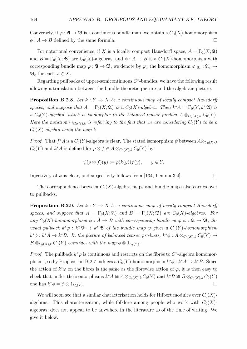
164 APPENDIX B. GROUPOIDS AND EQUIVARIANT KK-THEORY
Conversely, if ϕ : A→ B is a continuous bundle map, we obtain a C0(X)-homomorphism
φ : A→ B defined by the same formula.
For notational convenience, if X is a locally compact Hausdorff space, A = Γ0(X;A)
and B = Γ0(X;B) are C0(X)-algebras, and φ : A→ B is a C0(X)-homomorphism with
corresponding bundle map ϕ : A→ B, we denote by ϕx the homomorphism ϕ|Ax : Ax →Bx for each x ∈ X.
Regarding pullbacks of upper-semicontinuous C∗-bundles, we have the following result
allowing a translation between the bundle-theoretic picture and the algebraic picture.
Proposition B.2.8. Let k : Y → X be a continuous map of locally compact Hausdorff
spaces, and suppose that A = Γ0(X;A) is a C0(X)-algebra. Then k∗A = Γ0(Y ; k∗A) is
a C0(Y )-algebra, which is isomorphic to the balanced tensor product A ⊗C0(X),k C0(Y ).
Here the notation ⊗C0(X),k is referring to the fact that we are considering C0(Y ) to be a
C0(X)-algebra using the map k.
Proof. That f ∗A is a C0(Y )-algebra is clear. The stated isomorphism ψ betweenA⊗C0(X),k
C0(Y ) and k∗A is defined for ρ⊗ f ∈ A⊗C0(X),k C0(Y ) by
ψ(ρ⊗ f)(y) := ρ(k(y))f(y), y ∈ Y.
Injectivity of ψ is clear, and surjectivity follows from [134, Lemma 3.4].
The correspondence between C0(X)-algebra maps and bundle maps also carries over
to pullbacks.
Proposition B.2.9. Let k : Y → X be a continuous map of locally compact Hausdorff
spaces, and suppose that A = Γ0(X;A) and B = Γ0(X;B) are C0(X)-algebras. For
any C0(X)-homomorphism φ : A → B with corresponding bundle map ϕ : A → B, the
usual pullback k∗ϕ : k∗A → k∗B of the bundle map ϕ gives a C0(Y )-homomorphism
k∗φ : k∗A → k∗B. In the picture of balanced tensor products, k∗φ : A ⊗C0(X),k C0(Y ) →B ⊗C0(X),k C0(Y ) coincides with the map φ⊗ 1Cb(Y ).
Proof. The pullback k∗ϕ is continuous and restricts on the fibres to C∗-algebra homomor-
phisms, so by Proposition B.2.7 induces a C0(Y )-homomorphism k∗φ : k∗A→ k∗B. Since
the action of k∗ϕ on the fibres is the same as the fibrewise action of ϕ, it is then easy to
check that under the isomorphisms k∗A ∼= A⊗C0(X),k C0(Y ) and k∗B ∼= B⊗C0(X),k C0(Y )
one has k∗φ = φ⊗ 1Cb(Y ).
We will soon see that a similar characterisation holds for Hilbert modules over C0(X)-
algebras. This characterisation, while folklore among people who work with C0(X)-
algebras, does not appear to be anywhere in the literature as of the time of writing. We
give it below.

B.2. UPPER-SEMICONTINUOUS BUNDLES 165
Definition B.2.10. Let X be a locally compact Hausdorff space, and let pA : A→ X be
an upper-semicontinuous C∗-bundle. An upper-semicontinuous Hilbert-A-module-
bundle is an upper-semicontinuous Banach-bundle pE : E→ X such that
1. each Ex is a Hilbert Ax-module, with inner Ax-valued inner product denoted 〈·, ·〉x,
2. the map E×pE,pE E→ A given by (ex, fx) 7→ 〈ex, fx〉x, x ∈ X, is continuous,
3. the map E×pE,pA A → E obtained from the right action of the Ax on the Ex is
continuous.
For a C0(X)-algebra A = Γ0(X;A), it is clear that the sections E = Γ0(X;E) of an
upper-semicontinuous Hilbert A-module-bundle E form a Hilbert A-module under the
canonical pointwise operations, namely
〈ξ, η〉(x) := 〈ξ(x), η(x)〉x, x ∈ X
and
(ξ · ρ)(x) := ξ(x) · ρ(x), x ∈ X
for ξ, η ∈ Γ0(X;E) and ρ ∈ Γ0(X;A). The converse is also true.
Proposition B.2.11. Let X be a locally compact Hausdorff space and let A = Γ0(X;A)
be a C0(X)-algebra. If E is a Hilbert A-module, then there exists an upper-semicontinuous
Hilbert-A-module-bundle pE : E → X such that E is canonically isomorphic as a Hilbert
A-module to Γ0(X;E). Any adjointable operator T ∈ L(E,E ′) between Hilbert A-modules
E = Γ0(X;E) and E ′ = Γ0(X;E′) determines a bundle map T : E → E′ which resticts
on each Ex to an adjointable operator T x ∈ L(Ex,E′x), and vice versa.
Proof. For each x ∈ X, define the Hilbert Ax-module Ex := E ⊗A Ax, where Ax is
regarded as an A-module by ρ ·a := ρ(x)a for ρ ∈ A and a ∈ Ax. Then set E :=⊔x∈X Ex,
and define Γ := x 7→ e : e ∈ Ex. Apply Lemma B.2.3 to give a unique topology on E
for which Γ ⊂ Γ0(X;E), the canonical projection pE : E → X is open and continuous,
and for which fibrewise addition and scalar multiplication in each fibre are continuous.
We then must show that the maps E×pE,pE E 3 (e, f) 7→ 〈e, f〉 ∈ A and E×pE,pA A 3(e, a) 7→ e · a ∈ E are continuous. However both of these follow from the same argument
used in [152, Theorem C.25] to prove continuity of multiplication, using the facts that
‖〈e, f〉‖A ≤ ‖e‖E‖f‖E and ‖e · a‖E ≤ ‖e‖E‖a‖A for all (e, f) ∈ E×pE,pE E and (e, a) ∈E×pE,pA A.
We then have the analogues of Proposition B.2.8 and Proposition B.2.9.
Proposition B.2.12. Let X be a locally compact Hausdorff space, A = Γ0(X;A) a
C0(X)-algebra and E = Γ0(X;E) a Hilbert A-module. If Y is a locally compact Hausdorff
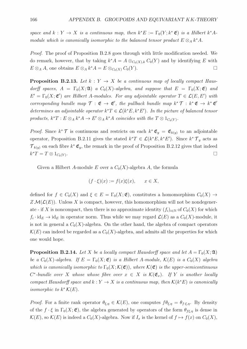
166 APPENDIX B. GROUPOIDS AND EQUIVARIANT KK-THEORY
space and k : Y → X is a continuous map, then k∗E := Γ0(Y ; k∗ E) is a Hilbert k∗A-
module which is canonically isomorphic to the balanced tensor product E ⊗A k∗A.
Proof. The proof of Proposition B.2.8 goes through with little modification needed. We
do remark, however, that by taking k∗A = A ⊗C0(X),k C0(Y ) and by identifying E with
E ⊗A A, one obtains E ⊗A k∗A = E ⊗C0(X) C0(Y ).
Proposition B.2.13. Let k : Y → X be a continuous map of locally compact Haus-
dorff spaces, A = Γ0(X;A) a C0(X)-algebra, and suppose that E = Γ0(X;E) and
E ′ = Γ0(X;E′) are Hilbert A-modules. For any adjointable operator T ∈ L(E,E ′) with
corresponding bundle map T : E → E′, the pullback bundle map k∗ T : k∗ E → k∗ E′
determines an adjointable operator k∗T ∈ L(k∗E, k∗E ′). In the picture of balanced tensor
products, k∗T : E ⊗A k∗A→ E ′ ⊗A k∗A coincides with the T ⊗ 1Cb(Y ).
Proof. Since k∗ T is continuous and restricts on each k∗ Ey = Ek(y) to an adjointable
operator, Proposition B.2.11 gives the stated k∗T ∈ L(k∗E, k∗E ′). Since k∗ T y acts as
T k(y) on each fibre k∗ Ey, the remark in the proof of Proposition B.2.12 gives that indeed
k∗T = T ⊗ 1Cb(Y ).
Given a Hilbert A-module E over a C0(X)-algebra A, the formula
(f · ξ)(x) := f(x)ξ(x), x ∈ X,
defined for f ∈ C0(X) and ξ ∈ E = Γ0(X;E), constitutes a homomorphism C0(X) →ZM(L(E)). Unless X is compact, however, this homomorphism will not be nondegener-
ate - if X is noncompact, then there is no approximate identity (fi)i∈N of C0(X) for which
fi · idE → idE in operator norm. Thus while we may regard L(E) as a C0(X)-module, it
is not in general a C0(X)-algebra. On the other hand, the algebra of compact operators
K(E) can indeed be regarded as a C0(X)-algebra, and admits all the properties for which
one would hope.
Proposition B.2.14. Let X be a locally compact Hausdorff space and let A = Γ0(X;A)
be a C0(X)-algebra. If E = Γ0(X;E) is a Hilbert A-module, K(E) is a C0(X) algebra
which is canonically isomorphic to Γ0(X;K(E)), where K(E) is the upper-semicontinuous
C∗-bundle over X whose whose fibre over x ∈ X is K(Ex). If Y is another locally
compact Hausdorff space and k : Y → X is a continuous map, then K(k∗E) is canonically
isomorphic to k∗K(E).
Proof. For a finite rank operator θξ,η ∈ K(E), one computes fθξ,η = θf ·ξ,η. By density
of the f · ξ in Γ0(X;E), the algebra generated by operators of the form θfξ,η is dense in
K(E), so K(E) is indeed a C0(X)-algebra. Now if Ix is the kernel of f 7→ f(x) on C0(X),

B.2. UPPER-SEMICONTINUOUS BUNDLES 167
then Ix · K(E) is the algebra generated by those θξ,η where ξ vanishes at the point x.
Then K(E)x := K(E)/(Ix · K(E)) can be identified with the algebra K(Ex) via the map
[θξ,η] 7→ θξ(x),η(x).
Well-definedness and injectivity are consequences of the fact that [θξ1,η1 ] = [θξ2,η2 ] if and
only if θξ1(x),η1(x) = θξ2(x),η2(x), while surjectivity is a result of there being “enough sections”
of Γ0(X;E) due to X being locally compact and Hausdorff. Applying Proposition B.2.7
gives the first part.
The second part is now a corollary of Propositions B.2.8 and B.2.7. Indeed, by
Proposition B.2.8, k∗K(E) is canonically isomorphic to Γ0(Y ; k∗K(E)), and we have a
continuous bundle isomorphism k∗K(E)→ K(k∗ E) of bundles over Y given by
(y, θe,f ) 7→ θ(y,e),(y,f), y ∈ Y, e, f ∈ Ek(y)
which clearly restricts to a C∗-isomorphism on each fibre. By Proposition B.2.7, the pull-
back k∗K(E) = Γ0(Y ; k∗K(E)) is then C0(X)-isomorphic to K(k∗E) = Γ0(Y ;K(k∗ E)).
Proposition B.2.14 tells us that when E is a Hilbert A-module over a C0(X)-algebra
A, any compact operator on E can be pulled back to a compact operator on k∗E, for
k : Y → X any continuous map of locally compact Hausdorff spaces. We have already
given a characterisation of the pullbacks of bounded adjointable operators by continuous
maps, but since we will be interested in unbounded representatives of KK-classes, we
end this section by establishing some basic facts about pullbacks of unbounded operators.
Proposition B.2.15. Let X be a locally compact Hausdorff space, A = Γ0(X;A) a
C0(X)-algebra, and E = Γ0(X;E), E ′ = Γ0(X;E′) are Hilbert A-module. Every A-linear
operator D : dom(D)→ E ′ on E determines a family Dxx∈X of operators on the fibres
of E which are linear over the respective fibres of A. If k : Y → X is a continuous map of
locally compact Hausdorff spaces, the k∗A-linear operator k∗D = D⊗1 on k∗E = E⊗Ak∗Adetermines a family Dyy∈Y on the fibres of k∗ E, where Dy = Dk(y) for all y ∈ Y .
Proof. For x ∈ X, define dom(Dx) := ξ(x) : ξ ∈ D(D). Then Dx : dom(Dx) → Ex
defined by
Dx(ξ(x)) := (Dξ)(x)
is an Ax-linear operator on Ex, and we obtain the family Dxx∈X . The second part
follows from the A-linearity of D, and a similar argument to the one just given.

168 APPENDIX B. GROUPOIDS AND EQUIVARIANT KK-THEORY
B.3 Groupoid actions on algebras and modules
We will always assume in this section that G is a locally compact, second countable,
locally Hausdorff groupoid with locally compact, Hausdorff unit space G(0).
Definition B.3.1. Let A = Γ0(G(0);A) be a C0(G(0))-algebra, where pA : A→ G(0) is an
upper-semicontinuous C∗-bundle over G(0). An action α of G on A consists of a family
αuu∈G such that
1. for each u ∈ G, αu : As(u) → Ar(u) is an isomorphism of C∗-algebras,
2. the map G ×s,pA A→ A defined by (u, a) 7→ αu(a) defines a continuous action of Gon A.
The triple (A,G, α) is called a groupoid dynamical system, and we say that A is a
G-algebra and that it admits a G-structure.
Let us consider the natural extension of Example B.2.6.
Example B.3.2. Let X be a G-space as in Definition B.1.3, with anchor map p : X →G(0). Then the C0(G(0))-algebra C0(X) is a G-algebra: for each u ∈ G, we have an
isomorphism αu : C0(Xs(u))→ C0(Xr(u)) defined by
αu(f)(x) := f(u−1 · x)
for all x ∈ Xr(u).
When G is Hausdorff, one defines an action α of G on a C0(G(0))-algebra A = Γ0(X;A)
as an isomorphism α : s∗A → r∗A of C0(G(0))-algebras, where s∗A = A ⊗C0(X),s C0(G)
and r∗A = A⊗C0(X),rC0(G), as in [115], which can by Proposition B.2.8 be identified with
Γ0(G; s∗A) and Γ0(G; r∗A) respectively. Unfortunately, lack of Hausdorff separability of
G in our examples means that a given bundle over G need not admit any interesting
globally continuous sections. Muhly and Williams get around this problem in the locally
Hausdorff setting by considering pullbacks over Hausdorff open subsets.
Lemma B.3.3. [134, Lemma 4.3] Suppose that (A,G, α) is a C∗-dynamical system, and
denote by A the C0(G(0))-algebra Γ0(G(0);A). If U ⊂ G is a Hausdorff open subset, then
for ρ ∈ s∗|UA the formula
αU(ρ)(u) := αu(ρ(u)), u ∈ U
defines a C0(U)-isomorphism of s|∗UA onto r|∗UA. If V ⊂ U is open, then by viewing s|∗VAas an ideal in s|∗UA, αV is the restriction of αU .
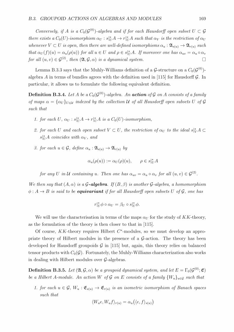
B.3. GROUPOID ACTIONS ON ALGEBRAS AND MODULES 169
Conversely, if A is a C0(G(0))-algebra and if for each Hausdorff open subset U ⊂ Gthere exists a C0(U)-isomorphism αU : s|∗UA→ r|∗UA such that αV is the restriction of αU
whenever V ⊂ U is open, then there are well-defined isomorphisms αu : As(u) → Ar(u) such
that αU(f)(u) = αu(ρ(u)) for all u ∈ U and ρ ∈ s|∗UA. If moreover one has αuv = αu αvfor all (u, v) ∈ G(2), then (A,G, α) is a dynamical system.
Lemma B.3.3 says that the Muhly-Williams definition of a G-structure on a C0(G(0))-
algebra A in terms of bundles agrees with the definition used in [115] for Hausdorff G. In
particular, it allows us to formulate the following equivalent definition.
Definition B.3.4. Let A be a C0(G(0))-algebra. An action of G on A consists of a family
of maps α = αUU∈U indexed by the collection U of all Hausdorff open subsets U of Gsuch that
1. for each U , αU : s|∗UA→ r|∗UA is a C0(U)-isomorphism,
2. for each U and each open subset V ⊂ U , the restriction of αU to the ideal s|∗VA ⊂s|∗UA coincides with αV , and
3. for each u ∈ G, define αu : As(u) → Ar(u) by
αu(ρ(u)) := αU(ρ)(u), ρ ∈ s|∗UA
for any U in U containing u. Then one has αuv = αu αv for all (u, v) ∈ G(2).
We then say that (A,α) is a G-algebra. If (B, β) is another G-algebra, a homomorphism
φ : A→ B is said to be equivariant if for all Hausdorff open subsets U of G, one has
r|∗Uφ αU = βU s|∗Uφ.
We will use the characterisation in terms of the maps αU for the study of KK-theory,
as the formulation of the theory is then closer to that in [115].
Of course, KK-theory requires Hilbert C∗-modules, so we must develop an appro-
priate theory of Hilbert modules in the presence of a G-action. The theory has been
developed for Hausdorff groupoids G in [115] but, again, this theory relies on balanced
tensor products with C0(G). Fortunately, the Muhly-Williams characterization also works
in dealing with Hilbert modules over G-algebras.
Definition B.3.5. Let (A,G, α) be a groupoid dynamical system, and let E = Γ0(G(0);E)
be a Hilbert A-module. An action W of G on E consists of a family Wuu∈G such that
1. for each u ∈ G, Wu : Es(u) → Er(u) is an isometric isomorphism of Banach spaces
such that
〈Wue,Wuf〉r(u) = αu(〈e, f〉s(u)
)

170 APPENDIX B. GROUPOIDS AND EQUIVARIANT KK-THEORY
for all e, f ∈ Es(u), and
2. the map G ×s,pE E → E defined by (u, e) 7→ Wue defines a continuous action of Gon E.
The tuple (E,A,G,W, α) is called a Hilbert module representation. We then say that
E is a G-Hilbert module and that E admits a G-structure.
The analogue of Lemma B.3.3 holds for Hilbert module representations virtually with-
out change to the proof.
Lemma B.3.6. Suppose (E,A,G,W, α) is a Hilbert module representation and denote
by E the G-Hilbert module Γ0(G(0);E). If U ⊂ G is a Hausdorff open subset, then for
ξ ∈ s|∗UE the formula
WU(ξ)(u) := Wu(ξ(u)), u ∈ U,
defines an isometric isomorphism of Banach spaces s∗|UE → r∗|UE. If V ⊂ U is open,
then by viewing s|∗VE as a sub-Hilbert module of s|∗UE over the ideal s|∗VA ⊂ s|∗UA, WV
is the restriction of WU .
Conversely, suppose that (A,α) is a G-algebra and E a Hilbert A-module. If for each
Hausdorff open subset U ⊂ G there exists an isometric isomorphism WU : s|∗UE → r|∗UE of
Banach spaces for which 〈WUξ,WUη〉 = αU(〈ξ, η〉) for all ξ, η ∈ s|∗UE, and such that WV
is the restriction of WU whenever V ⊂ U is open, then there are isometric isomorphisms
Wu : Es(u) → Er(u) of Banach spaces such that WU(ξ)(u) = Wu(ξ(u)) for all u ∈ U and
ξ ∈ s|∗UE. If moreover one has Wuv = Wu Wv for all (u, v) ∈ G(2), then (E,A,G,W, α)
is a Hilbert module representation.
Again, since we will be using the algebraic picture in KK-theory, we give the equiv-
alent definition formulated in the language of [115].
Definition B.3.7. Let (A,α) be a G-algebra and let E be a Hilbert A-module. An action
of G on E consists of a family of maps W = WUU∈U indexed by the collection U of all
Hausdorff open subsets U of G such that
1. for each U , WU : s|∗UE → r|∗UE is an isometric isomorphism of Banach spaces, for
which 〈WUξ,WUη〉 = αU(〈ξ, η〉) for all ξ, η ∈ s|∗UE,
2. for each U and each open subset V ⊂ U , the restriction of WU to the sub-Hilbert
module s|∗VE over the ideal s|∗VA ⊂ s|∗UA coincides with WV , and
3. for each u ∈ G, definine Wu : Es(u) → Er(u) by
Wu(ξ(u)) := WU(ξ)(u), ξ ∈ s|∗UE
for any U in U containing u. Then one has one has Wuv = Wu Wv for all
(u, v) ∈ G(2).

B.4. KKG-THEORY 171
We then say that (E,W ) is a G-Hilbert A-module. If (E,W ) and (E ′,W ′) are two
G-Hilbert A-modules, we say that a map T ∈ L(E,E ′) is equivariant if for all Hausdorff
open subsets U of G, one has
W ′U s|∗UT = r|∗UT WU ,
where s|∗UT and r|∗UT are the pullbacks defined in Proposition B.2.15.
We give one final definition before going into KKG-theory.
Definition B.3.8. Let (E,W ) be a G-Hilbert B-module over a G-algebra (B, β), and
suppose that (A,α) is another G-algebra. We say that a representation π : A→ L(E) is
equivariant if for every Hausdorff open subset U ⊂ G we have
AdWU(πsU(a)) = πrU(αU(a))
for all a ∈ A. Here πsU := π ⊗ 1Cb(U) and πrU := π ⊗ 1Cb(U) are respectively the induced
homomorphisms s|∗UA = A⊗C0(G(0)),sC0(U)→ L(s∗|U E) and r|∗UA = A⊗C0(G(0)),rC0(U)→L(r∗|U E).
B.4 KKG-theory
We now present a generalization of the theory in [115] to the setting of the locally compact,
locally Hausdorff groupoids of foliation theory. We assume from here that all algebras and
Hilbert modules are Z2-graded. For all Hausdorff open subsets U ⊂ G, C0(U) is assumed
to be trivially graded. If (A.α) is any G-algebra, the isomorphisms αU : s|∗UA → r|∗UAare assumed to preserve the grading on A, and for all G-Hilbert A-modules (E,W ), the
isomorphisms WU : s|∗UE → r|∗UE are assumed to be of degree 0 with respect to the
grading on E.
Definition B.4.1. Let (A,α) and (B, β) be G-C∗-algebras. A G-equivariant Kasparov
A-B-module is a triple (E, π, F ), where (E,W ) is a G-equivariant Hilbert B-module car-
rying an equivariant representation π : A→ L(E), and where F ∈ L(E) is homogeneous
of degree 1 such that for all a ∈ A one has
1. a(F − F ∗) ∈ K(E),
2. a(F 2 − 1) ∈ K(E),
3. [F, a] ∈ K(E),
and such that for all Hausdorff open subsets U of G and for all a′ ∈ r|∗UA one has
4. a′(WU s|∗UF W−1U − r|∗UF ) ∈ r|∗U K(E).

172 APPENDIX B. GROUPOIDS AND EQUIVARIANT KK-THEORY
We say that two G-equivariant Kasparov A-B-modules (E, π, F ) and (E, π′, F ′) are uni-
tarily equivalent if there exists a G-equivariant unitary V : E → E ′ of degree 0 such
that V FV ∗ = F ′ and V π(a)V ∗ = π′(a) for all a ∈ A. We denote by EG(A,B) the set of
all unitary equivalence classes of G-equivariant Kasparov A-B-modules.
Now let (B, β) be a G-algebra, and consider the algebra B ⊗ C([0, 1]). This algebra
admits the nondegenerate homomorphism ·⊗1[0,1] : C0(X)→ ZM(B⊗C([0, 1])), as well
as the G-structure βU : (s|∗UB)⊗C([0, 1])→ (r|∗UB)⊗C([0, 1]) defined for each Hausdorff
open subset U of G by
βU(b⊗ f) := β(b)⊗ f,
for b ∈ s|∗UB and f ∈ C([0, 1]). Moreover, for any t ∈ [0, 1], the evaluation functional
f 7→ f(t) on C([0, 1]) maps B⊗C([0, 1]) to B in an equivariant manner. The equivalence
relation thus induced by homotopy ∼h on Kasparov modules can thus be formulated in
the same way as in [115].
Definition B.4.2. We denote by KKG(A,B) the set of ∼h-equivalence classes of ele-
ments in EG(A,B).
As we would expect, KKG(A,B) is indeed an abelian group for all G-algebras A and
B. As is usual in KK theories, we define the notion of degeneracy.
Definition B.4.3. An element (E, π, F ) of EG(A,B) is said to be degenerate if for all
a ∈ A one has
1. a(F 2 − 1) = 0,
2. [F, a] = 0,
and if for all Hausdorff open subsets U of G one has
3. WU s|∗UF W−1U = r|∗UF .
Proposition B.4.4. Under the direct sum, KKG(A,B) is an abelian group.
Proof. A similar proof to that in [115, Proposition 4.1.1] applies, using the pullbacks over
Hausdorff open subsets instead of pullbacks over all of G, and using Definition B.4.3 for
degenerate Kasparov modules.
Functoriality over G-equivariant maps in KKG goes through in the same way as in
[115] as well, provided one uses the slightly generalised notion of equivariance given in
Definition B.3.4.

B.4. KKG-THEORY 173
Proposition B.4.5. Let A, B, and C be G-algebras.
1. any homomorphism φ : A→ C determines a homomorphism
φ∗ : KKG(C,B)→ KKG(A,B),
of abelian groups, and
2. any homomorphism ψ : B → C determines a homomorphism
ψ∗ : KKG(A,B)→ KKG(A,C)
of abelian groups.
We end the section with a final definition and result on unbounded representatives,
which are slight modifications of those found in [139].
Definition B.4.6. Let A and B be G-algebras. An unbounded equivariant Kasparov
A-B-module is a triple (A, πE,D), where A is a dense ∗-G-subalgebra of A, (E,W ) is
a G-Hilbert B-module carrying an equivariant representation π : A → L(E), and where
D is a densely defined, self-adjoint and regular operator on E of degree 1 such that
1. π(a)(1 +D2)−12 ∈ K(E) for all a ∈ A,
2. for all a ∈ A, the operator [D, a] extends to an element of L(E), and for all Haus-
dorff open subsets U of G and all f ∈ Cc(U) one has
f r|∗Ua (WU s|∗UD W−1U − r|
∗UD) ∈ L(r|∗UE)
and
f s|∗Ua (W−1U r|
∗UD WU − s|∗UD) ∈ L(s|∗UE),
3. for all Hausdorff open subsets U of G and for all f ∈ Cc(U), one has dom(r|∗UD f) = WU dom(s|∗UD f).
Proposition B.4.7. Let A and B be G-algebras. Every unbounded equivariant Kasparov
A-B-module (A, πE,D) determines a G-equivariant Kasparov A-B-module (E, π,D(1 +
D2)−12 ), defining a class [D] ∈ KKG(A,B).
Proof. By the same arguments as in the non-equivariant case [13], the triple (E, π,D(1+
D2)−12 ) satisfies items 1., 2. and 3. of Definition B.4.1. The final item 4. in Definition
B.4.1 follows by restricting [139, Theoreme 6] to each of the Hausdorff open subsets U in
G.
174 APPENDIX B. GROUPOIDS AND EQUIVARIANT KK-THEORY
B.5 The Kasparov product
The characteristic feature of KK-theory is the Kasparov product. In [115], it is proved
that when G is Hausdorff, for all G-algebras A, D, B there is an associative and non-trivial
product
KKG(A,D)×KKG(D,B)→ KKG(A,B).
The same is true when G is locally Hausdorff. Provided that one replaces the notion of
an equivariant Kasparov module used in [115] with the more general definition for locally
Hausdorff G that we have been using here, the proof of this fact is essentially the same
as the one presented in [115]. Since the proof is, however, quite technical, we will outline
each individual result used in the proof and explain precisely what must be changed in
this more general setting.
Lemma B.5.1 (Existence of quasi-central approximate units). Let (J, α) be a Z2-graded
G-algebra. Let Uii∈N be a countable base for the topology of G. Since G is locally
Hausdorff, every Ui must be Hausdorff. For each i choose ϕi ∈ C0(Ui) and let hi ∈ r|∗UiJ .
Then, for all h0, h ∈ J with h0 ≥ 0 of degree 0 and ‖h0‖ ≤ 1, for all strictly compact
subsets K of M(J) and for all ε > 0, there exists an element u ∈ J of degree 0 such that
1. h0 ≤ u, ‖u‖ ≤ 1,
2. ‖uh− h‖ ≤ ε,
3. for all d ∈ K, ‖[d, u]‖ ≤ ε,
and for all i ∈ N
4. ‖(1⊗r|Ui ϕi)(αUi(u⊗s|Ui 1)− u⊗r|Ui 1)‖ ≤ ε, and
5. ‖αUi(1− u⊗s|Ui 1)hi‖ ≤ ε.
Proof. The proof is similar to that of [115, Lemme 5.1.1]. One defines
J ′ := J ⊕ C(K; J)⊕(⊕
i∈N
r|∗UiJ)⊕(⊕
i∈N
r|∗UiJ)
and then defines a linear map Φ : J → J ′ that sends x ∈ J to(xh−h, (d 7→ [d, x]), (1⊗r|Ui ϕi)(αUi(x⊗s|Ui 1)−x⊗r|Ui 1))i∈N, (αUi(1−x⊗s|Ui 1)h′)i∈N
).
The argument in [115, Lemme 5.1.1] shows that Φ extends to a strictly continuous map
M(J) → M(J ′), and that 0 is in the norm closure of Φ(C), where C = x ∈ J :
deg(x) = 0, h0 ≤ x < 1. Since C contains an approximate identity for J , one can always
find u ∈ C that is close to 1 ∈M(J). Since Φ(1) = 0 is in the norm closure of Φ(C), the
desired estimates for u follow.

B.5. THE KASPAROV PRODUCT 175
The existence of quasi-central approximate units is used in the proof of Kasparov’s
technical lemma below.
Theorem B.5.2 (Kasparov’s technical lemma). Let (A,α) be a G-algebra. Let J be a
G-subalgebra and an ideal of A, let F be a separable vector subspace of M(A), and let a
be a positive element of M(J) such that aA ⊂ J .
Let Uii∈N be a countable base for the topology of G. For each i ∈ N, let a′i be a positive
element of M(r|∗UiJ) such that (r|∗UiA)a′i ∈ r|∗UiJ , and let χi be a strictly positive element
of C0(Ui). Then there exists M ∈ M(A) homogeneous of degree 0 with 0 < M < 1 such
that
1. (1−M)a ∈ J ,
2. MA ⊂ J ,
3. [F ,M ] ⊂ J ,
and such that for all i ∈ N,
4. (1⊗r|Ui χi)(αUi(M ⊗s|Ui 1)−M ⊗r|Ui 1) ∈ r|∗UiJ , and
5. (1⊗r|Ui χi)α((1−M)⊗s|Ui 1)a′i ∈ r|∗UiJ .
Proof. The proof is the same as in [115, Theoreme 5.1.1], using Lemma B.5.1 instead of
[115, Lemme 5.1.1].
We recall here the notion of a connection given by Connes and Skandalis [61]. Let
A and B be C∗-algebras, and suppose that E1 is a Hilbert A-module, E2 is a Hilbert
B-module, and that π : A→ L(E2) is a representation. Let E = E1 ⊗π E2, and for each
ξ ∈ E1 we denote by Tξ ∈ L(E2, E) defined by
Tξη := ξ ⊗ η, η ∈ E2.
The adjoint of Tξ is given on η ⊗ ζ ∈ E by
T ∗ξ (η ⊗ ζ) = π(〈ξ, η〉)ζ.
If F2 ∈ L(E2), we say that an operator F ∈ L(E) is an F2-connection for E1 if for all
ξ ∈ E1, one has
TξF2 − (−1)deg(ξ) deg(F2)FTξ ∈ K(E2, E),
and
F2T∗ξ − (−1)deg(ξ) deg(F2)T ∗ξ F ∈ K(E,E2).
If E1 is countably generated and [F2, π(A)] ⊂ K(E), then the algebra L(E) contains an
F2-connection for E1.

176 APPENDIX B. GROUPOIDS AND EQUIVARIANT KK-THEORY
Proposition B.5.3. Let A and B be G-algebras, let E1 be a G-equivariant Hilbert A
module, and let (E2, π2, F2) be an equivariant Kasparov A-B-module. Define E := E1⊗π2
E2. Define π : K(E1) → L(E) by π(T ) := T ⊗ idE1 and let F be an F2-connection of
degree 1 for E1. Then the triple (E, π, F ) is a G-equivariant Kasparov K(E1)-B-module.
Proof. That the triple (E, π, F ) defines a Kasparov module is a consequence of [61, Propo-
sition A.2]. That the module is equivariant in the sense of Definition B.4.1 follows by a
similar argument to the one given in [115]. More specifically, for each Hausdorff open sub-
set U of G, the representation π : K(E1) → L(E) lifts to πU : r|∗U K(E1) = K(r|∗UE1) →L(r|∗UE), and then the argument in [115, Proposition 5.1.1] can be used to show that
(WU s|∗UF W−1U − r|
∗UF )πU(θ) ∈ K(r|∗UE), θ ∈ r|∗U K(E1),
where WU : s|∗UE → r|∗UE is the G-structure on E induced by the G-structures on E1 and
E2. Since this can be done for any Hausdorff open subset U of G, it follows that (E, π, F )
does indeed define an equivariant Kasparov K(E1)-B-module.
To prove existence and uniqueness of the Kasparov product, we will need to employ
Theorem B.5.2. Observe however that Theorem B.5.2 concerns a fixed countable base for
the topology of G, and a-priori says nothing about arbitrary Hausdorff open subsets of G.
Since our definition of equivariance is concerned with behaviour over arbitrary Hausdorff
subsets, we will need the following simple lemma.
Lemma B.5.4. Let Uii∈N be a countable base of Hausdorff open subsets for the second
countable topological space G, and suppose that A is a G-algebra. Then if U is any
Hausdorff open subset of G, and IU ⊂ N is an indexing set such that⋃i∈IU Ui = U , any
aU ∈ r|∗UA can be written as a norm-convergent infinite sum∑
i∈IU aUi, where aUi ∈ r|∗UiAfor all i ∈ N. Conversely, any such norm-convergent infinite sum has an element of r|∗UAas its limit.
Proof. It will be useful to consider the bundle-theoretic picture. Thus A = Γ0(G(0);A) for
some upper-semicontinuous C∗-bundle A → G(0). Since U is locally compact, Hausdorff
and second countable, it is paracompact, and so the open cover Uii∈IU of U admits
a partition of unity ϕi ∈ C0(Ui)i∈IU . Then for any aU ∈ Γ0(U ; r|∗U A) we can write
aU =∑∈IU ϕiaU , which gives the first claim.
For the second, simply observe that because every r|∗UiA is contained in r|∗UA, any
norm-convergent infinite sum of elements of the r|∗UiA gives a Cauchy sequence of partial
sums of elements of r|∗UA, which by completeness of r|∗UA must converge to an element
of r|∗UA.
Finally we come to existence and uniqueness of the Kasparov product.

B.5. THE KASPAROV PRODUCT 177
Theorem B.5.5 (Existence). Let A, B and D be G-algebras, and suppose (E1, π1, F1) ∈EG(A,D) and (E2, π2, F2) ∈ EG(D,B). Let E := E1 ⊗π2 E2 and let π := π1 ⊗ idE2 :
A → L(E), so that (E, π) is an equivariant A-B-bimodule. Let F1]F2 denote the set of
F ∈ L(E) such that
1. (E, π, F ) ∈ EG(A,B),
2. F is an F2-connection for E1,
3. for all a ∈ A, π(a)[F1 ⊗π2 1E2 , F ]π(a∗) is positive modulo K(E).
Then F1]F2 is nonempty.
Proof. Choose an F2-connection T for E1 and denote
J := K(E),
A1 := K(E) +K(E1)⊗ idE2 .
Thus J is an ideal and a G-subalgebra of the G-algebra A1. Take
F := VectF1 ⊗ idE2 , T, π(A)
to be the separable subspace ofM(A1) generated by F1⊗ idE2 , T and π(a) for all a ∈ A.
Finally denote by A2 the subalgebra of L(E) generated by T − T ∗, T 2 − 1, [T, F1 ⊗ idE2 ]
and [T, π(A)], and let a2 ∈ A2 ⊂M(A1) be strictly positive.
Now let Uii∈N be a countable base of Hausdorff open neighbourhoods for the topol-
ogy of G, and for each i ∈ N let χi ∈ C0(Ui), and let a′i be a strictly positive element
of the algebra generated by WUi s|∗UiT W−1Ui− r|∗UiT . By Proposition B.5.3, we have
(r|∗Ui K(E1)⊗ idE2)a′i ∈ r|∗UiJ and hence (r|∗UiA1)a′i ∈ r|∗UiJ for all i ∈ N.
We can thus apply Theorem B.5.2 to obtain M ∈M(A1) with the stated properties.
In particular, since (1 −M)a2 ∈ J and a2 is strictly positive (so that a2A2 is dense in
A2), we have (1−M)A2 ⊂ J . By setting
F := M12 (F1 ⊗π2 idE2) + (1−M)
12T,
the usual arguments for non-equivariant KK-theory [104, Section 4, Theorem 4] show
that (E, π, F ) is a (non-equivariant) Kasparov A-B-module and that F satisfies properties
(2) and (3) of the theorem statement. It remains therefore to prove that (E, π, F ) is G-
equivariant.
The arguments used in [115, Theorem 5.2.1] show that for each i ∈ N and each
a′Ui ∈ r|∗UiA, one has
a′Ui(WUi s|∗UiF W−1Ui− r|∗UiF ) ∈ r|∗Ui K(E). (B.1)
178 APPENDIX B. GROUPOIDS AND EQUIVARIANT KK-THEORY
Any other Hausdorff open subset U of G can be written as U =⋃i∈IU⊂N Ui for some
subset IU ⊂ N, and using Lemma B.5.4, we know that any a′U ∈ r|∗UA can be written as
a norm-convergent sum
a′U =∑i∈IU
a′Ui ,
where for each i ∈ N, aUi ∈ r|∗UiA. In particular, we can write
a′U(WU s|∗UF W−1U − r|
∗UF ) =
∑i∈IU
a′Ui(WUi s|∗UiF W−1Ui− r|∗UiF ),
which by (B.1) is a norm-convergent sum of elements of r|∗Ui K(E), whose sum is then by
Lemma B.5.4 an element of r|∗U K(E). Thus (E, π, F ) is indeed an element of EG(A,B).
Theorem B.5.6 (Uniqueness). In the setting of the previous theorem, if F, F ′ ∈ F1]F2,
then (E, π, F ) and (E, π, F ′) define the same class in KKG(A,B), and we refer to this
class as the Kasparov product of (E1, π1, F1) and (E2, π2, F2).
Proof. Uniqueness can be seen using the proof of [147, Theorem 12] together with The-
orem B.5.2 and the partition of unity argument used in the proof of existence.
B.6 Crossed products
We now must discuss crossed products of G-algebras as well as their relationship to KKG-
theory. We will continue to assume in this section that G is a locally compact, second
countable, locally Hausdorff groupoid with locally compact Hausdorff unit space G(0). In
addition, we will assume that G is equipped with a Haar system.
Definition B.6.1. A Haar system on G is a family λxx∈G(0) of measures on G such
that each λx is supported on Gx, and is a regular Borel measure thereon, and such that
1. for all v ∈ G and f ∈ Cc(G) one has∫Gf(vu) dλs(v)(u) =
∫Gf(u) dλr(v)(u)
and,
2. for each f ∈ Cc(G), the map
x 7→∫Gf(u) dλx(u)
is continuous with compact support on G.

B.6. CROSSED PRODUCTS 179
That G admits a Haar system is a nontrivial requirement in general. Indeed, if G ad-
mits a Haar system then its range and source maps must be open [136, Proposition 2.2.1],
and it is not difficult to find examples of locally compact (even Hausdorff) groupoids for
which this is not the case [144, Section 3]. In the context of a foliated manifold, any choice
of leafwise half-density determines a Haar system on the associated holonomy groupoid
(see Definition 3.3.1).
Importantly, when G has a Haar system we can construct a crossed product algebra
from any G-algebra A = Γ0(G(0);A). For any Hausdorff open subset U of G, we denote
by Γc(U ; r∗A) the space of compactly supported continuous sections of the bundle r∗A
over U , extended by zero outside of U to a (not necessarily continuous) function on G.
We define Γc(G; r∗A) to be the subspace of sections of r∗A over G that are spanned by
elements of Γc(U ; r∗A) as U varies over all Hausdorff open subsets of G.
Remark B.6.2. If G is a Lie groupoid (such as the holonomy groupoid of a foliation),
then we can take smooth sections, denoted Γ∞c , instead of continuous sections.
Proposition B.6.3. [134, Proposition 4.4] If (A,G, α) is a groupoid dynamical system,
the space Γc(G; r∗A) is a ∗-algebra with respect to the convolution product and adjoint
given respectively by
f ∗ g(u) :=
∫Gf(v)αv
(g(v−1u)
)dλr(u)(v) f ∗(u) := αu(f(u−1)∗)
for all f, g ∈ Γc(G; r∗A) and u ∈ G.
Remark B.6.4. Note that one could also define a ∗-algebra structure on the space
Γc(G; s∗A) obtained by pulling back A via the source map. In this case, the multiplication
and involution are given by
f ∗ g(u) :=
∫Gαw(f(uw)
)g(w−1) dλs(u)(w), f ∗(u) := αu−1
(f(u−1)∗
).
Moreover, the map f 7→ α f defines an isomorphism Γc(G; s∗A) → Γc(G; r∗A) of ∗-algebras. While Γc(G; s∗A) is in a certain sense the more natural object to consider for
left actions of groupoids, we choose to work with pullbacks over the range in accordance
with [118].
The reduced C∗-algebra of G is obtained from the algebra Cc(G) by completing it with
respect to the norm obtained from the canonical family of ∗-representations πx : Cc(G)→L(L2(Gx)), x ∈ G(0). For a groupoid dynamical system (A,G, α) the situation is slightly
more complicated - namely, we must complete the convolution algebra Γc(G; r∗A) with
respect to the norm obtained from a particular family Hilbert modules constructed from
A.

180 APPENDIX B. GROUPOIDS AND EQUIVARIANT KK-THEORY
Proposition B.6.5. Let (A,G, α) be a groupoid dynamical system. Then for each x ∈G(0), the completion L2(Gx; r∗A) of Γc(Gx; r∗A) in the Ax-valued inner product
〈ξ, η〉x := (ξ∗ ∗ η)(x) =
∫Gαu(ξ(u−1)∗η(u−1)
)dλx(u),
defined for ξ, η ∈ Γc(Gx; r∗A), is a Hilbert Ax-module, with right Ax-action given by
(ξ · a)(u) := ξ(u)αu(a), u ∈ Gx
for all ξ ∈ Γc(Gx; r∗A) and a ∈ Ax.
Moreover, for each x ∈ G(0), a representation πx : Γc(G; r∗A) → L(L2(Gx; r∗A)
)is
defined by the formula
πx(f)ξ(u) := f ∗ ξ(u) =
∫Gf(v)αv
(ξ(v−1u)
)dλr(u)(v), u ∈ Gx
for f ∈ Γc(G; r∗A) and ξ ∈ Γc(Gx; r∗A).
Proof. It is clear from inspection that for x ∈ G(0), ξ, η ∈ Γc(Gx; r∗A) and a ∈ Ax, the
formulae defining 〈ξ, η〉x and (ξ · a) make sense. Moreover, we have
〈ξ, η〉∗x = (ξ∗ ∗ η)∗(x) = (η∗ ∗ ξ)(x) = 〈η, ξ〉x
since ∗ is an involution, and
〈ξ, η · a〉x =
∫Gαu(ξ(u−1)∗(η · a)(u−1)
)dλx(u)
=
∫Gα(u)
(ξ(u−1)∗η(u−1)αu(a)
)dλx(u) = 〈ξ, η〉xa
since αu−1 = α−1u as C∗-isomorphisms. Consequently [113, Page 4], the completion
L2(Gx; r∗A) is indeed a Hilbert Ax-module.
The extension of πx to a representation πx : Γc(G; r∗A) → L(L2(Gx; r∗A)
)follows
from the argument of Koshkam and Skandalis [107, 3.6]. Specifically, Koshkam and
Skandalis show that for f ∈ Γc(G; s∗A) (see Remark B.6.4) and ξ ∈ Γc(Gx;Ax), the
formula
πx(f)ξ(u) :=
∫Gαw(f(uw)
)ξ(w−1) dλs(u)(w), u ∈ Gx
extends to a representation πx : Γc(G; s∗A) → L(L2(Gx;Ax)
), where L2(Gx;Ax) is the
Hilbert Ax-module that is the completion of Γc(Gx;Ax) in the Ax-valued inner product
〈ξ, η〉x :=∫G ξ(u
−1)∗η(u−1) dλx(u). Observe that the map Ux : Γc(Gx;Ax)→ Γc(Gx; r∗A)
defined by (Uxξ)(u) := αu
(ξ(u)
)
B.6. CROSSED PRODUCTS 181
satisfies(Ux(ξ · a)
)(u) = αu(ξ(u))αu(a) =
(Uxξ)· a(u) for all a ∈ Ax, ξ ∈ Γc(Gx;Ax) and
u ∈ Gx, and satisfies
〈Uxξ, η〉x =
∫Gαu((Uxξ)(u
−1)∗η(u−1))dλx(u) =
∫Gξ(u−1)∗αu
(η(u−1)
)dλx(u)
=
∫Gξ(u−1)∗
(U−1x η)(u−1) dλx(u) = 〈ξ, U−1
x η〉x
for all ξ ∈ Γc(Gx;Ax) and η ∈ Γc(Gx; r∗A). Thus it extends to a unitary isomorphism
Ux : L2(Gx;Ax)→ L2(Gx; r∗A) of Hilbert Ax-modules. Now we observe that
(Ux πx(f) U∗x
)ξ(u) =αu
((πx(f) U∗x
)ξ(u)
)=αu
(∫Gαw(f(uw)
)(U∗xξ
)(w−1) dλx(w)
)=αu
(∫Gαw(f(uw)
)αw(ξ(w−1)
)dλx(w)
)=
∫Gαuw
(f(uw)
)αuw
(ξ(w−1)
)dλx(w)
=
∫Gαv(f(v)
)αv(ξ(v−1u)
)dλr(u)(v) = πx
(α f
)ξ(u)
for any ξ ∈ Γc(Gx; r∗A), so that πx is unitarily equivalent to the representation πx and is
consequently itself a representation by [107, 3.6].
Completing in the norm obtained from the Hilbert module representations of Propo-
sition B.6.5 we obtain the reduced crossed product algebra.
Definition B.6.6. The completion Aor G of Γc(G; r∗A) in the norm
‖f‖AorG := supx∈G(0)
‖πx(f)‖L2(Gx;r∗ A)
is a C∗-algebra called the reduced crossed product algebra associated to the dynamical
system (A,G, α).
Remark B.6.7. The proof of Proposition B.6.5 together with [107, 3.7] implies that the
C∗-algebra defined in Definition B.6.6 coincides with that given in [107].
Let us consider now the crossed product obtained from Example B.3.2.
Example B.6.8. Let X be a G-space as in Definition B.1.3, with associated G-algebra
C0(X). Denote the corresponding field of C∗-algebras over G(0) by C0(X), so that
C0(X)r(u) = C0(Xr(u)) for all u ∈ G. Then an element f of Γc(G; r∗ C0(X)) is a continu-
ously varying and compactly supported assignment to each element u of some Hausdorff
open subset U of G an element fu ∈ C0(Xr(u)).

182 APPENDIX B. GROUPOIDS AND EQUIVARIANT KK-THEORY
Consider now the ∗-algebra Cc(X o G) obtained from the locally compact, second
countable, locally Hausdorff groupoid X o G with unit space X (see the discussion im-
mediately following Definition B.1.3), whose operations are defined by
f ∗ g(x, u) :=
∫Gf(x, v)g(v−1 · x, v−1u) dλr(u)(v), f ∗(x, u) := f(u−1 · x, u−1).
Any f ∈ defines an element f ∈ Γc(G; r∗ C0(X)) by the formula
fu(x) := f(x, u),
and it is easily seen by direct calculation that f 7→ f is a homomorphism of ∗-algebras.
Idenfifying Cc(X o G) with its image in Γc(G; r∗A) in this way, by density of Cc(Xr(u))
in C0(Xr(u)) for each u ∈ G we see that Cc(X o G) is a dense subalgebra of C0(X) or G.
Thus we write fu(x) for f ∈ Cc(X o G) evaluated on (x, u) ∈ X o G.
B.7 The descent map
We now prove that Kasparov’s descent map [105] exists and continues to function as
expected in the equivariant setting for locally Hausdorff groupoids. While the relevant
definitions in the Hausdorff case [115] are relatively simple using balanced tensor products,
in the locally Hausdorff case one must use the bundle picture, which requires slightly more
work. Once these definitions are established, however, establishing the descent map and
its properties is much the same as in the Hausdorff case.
Suppose that we are given a G-algebra (B = Γ0(G; r∗B), β) and a G-Hilbert B-module
(E = Γ0(G(0); r∗ E),W ). We take Γc(G; r∗ E) to be the subspace of sections of r∗ E over Gthat are spanned by elements of Γc(U ; r∗ E) as U varies over all Hausdorff open subsets
of G. Observe that Γc(G; r∗ E) admits the Γc(G; r∗B)-valued inner product
〈ξ, ξ′〉G(u) :=
∫Gβv(〈ξ(v−1), ξ′(v−1u)〉s(v)
)dλr(u)(v), u ∈ G
for ξ, ξ′ ∈ Γc(G; r∗ E), which is positive by [134, Proposition 6.8] and the argument given
in [152, p. 116]. The space Γc(G; r∗ E) also admits a right action of Γc(G; r∗B) given by
(ξ · f)(u) :=
∫Gξ(v) · βv
(f(v−1u)
)dλr(u)(v), u ∈ G
for ξ ∈ Γc(G; r∗ E) and f ∈ Γc(G; r∗B), with · denoting the (fibrewise) right action of
B on E. By completing in the norm attained from the reduced C∗-algebra B or G we
obtain [113, Page 4] a Hilbert B or G-module.
Definition B.7.1. Given a G-algebra (B = Γ0(G(0);B), β) and a G-Hilbert B-module

B.7. THE DESCENT MAP 183
(E = Γ0(G(0); r∗ E),W ), we define Eor G to be the completion of Γc(G; r∗ E) in the norm
‖ξ‖EorG := ‖〈ξ, ξ〉G‖12BorG.
The space E or G is a Hilbert B or G-module, which we will refer to as the crossed
product of E by G.
We will need to pull back operators on equivariant modules to their crossed products
as follows.
Proposition B.7.2. Let (B = Γ0(G(0);B), β) be a G-algebra and let (E = Γ0(G(0);E),W )
be a G-Hilbert B-module. Given T ∈ L(E), the operator r∗(T ) defined on Γc(G; r∗ E)
defined by (r∗(T )ξ
)(u) := Tr(u)ξ(u)
extends to an operator r∗(T ) ∈ L(E or G). When G is Hausdorff, r∗(T ) ∈ L(E or G)
defined in this manner coincides with the operator T ⊗ 1 on E or G ∼= E ⊗B (B or G) as
in [115, p. 75].
Proof. That r∗(T ) is Γc(G; r∗B)-linear is clear by the B-linearity of T . Moreover, for any
ξ ∈ Γc(G; r∗ E) we have
〈r∗(T )ξ, r∗(T )ξ〉G(u) =
∫Gβv(〈Ts(v)ξ(v
−1), Ts(v)ξ(v−1u)〉s(v)
)dλr(u)(v)
≤∫G‖Ts(v)‖2
Es(v)βv(〈ξ(v−1), ξ(v−1u)〉s(v)
)dλr(u)(v)
≤ supx∈G(0)
‖Tx‖2Ex
∫Gβv(〈ξ(v−1), ξ(v−1u)
)dλr(u)(v),
from which we deduce that ‖r∗(T )ξ‖EorG ≤ ‖T‖L(E)‖ξ‖EorG. Consequently, r∗(T ) ex-
tends to a B or G-linear operator on all of E or G. It is then easily checked that r∗(T )
is adjointable, with adjoint r∗(T ∗).
The final claim follows from the fact that T ⊗ 1 on E ⊗B (B or G) agrees with r∗(T )
on the dense subspace Γc(G; r∗ E) of E ⊗B (B or G).
Moreover one can take the crossed product of an equivariant representation.
Proposition B.7.3. Let (A = Γ0(G(0);A), α) and (B = Γ0(G(0);B), β) be G-algebras and
let (E = Γ0(G(0);E),W ) be a G-Hilbert module. Then if π : A→ L(E) is an equivariant
representation, the formula
(π or G)(f)ξ(u) :=
∫Gπr(v)(f(v))Wv
(ξ(v−1u)
)dλr(u)(v), u ∈ G
defined for f ∈ Γc(G; r∗A) and ξ ∈ Γc(G; r∗ E) determines a representation π or G :
Aor G → L(E or G).

184 APPENDIX B. GROUPOIDS AND EQUIVARIANT KK-THEORY
Proof. First observe that πor G is ∗-preserving in the sense that for any f ∈ Γc(G; r∗A),
and ξ, ξ′ ∈ Γc(G; r∗ E), the element 〈(π or G)(f)ξ, ξ′〉G(u) of Br(u) is equal to∫G
∫Gβv(〈πs(v)(f(w))Ww
(ξ(w−1v−1)
), ξ′(v−1u)〉s(v)
)dλs(v)(w) dλr(u)(v)
=
∫G
∫Gβv(〈Ww
(ξ(w−1v−1)
), πs(v)(f(w)∗)ξ′(v−1u)〉s(v)
)dλs(v)(w) dλr(u)(v)
=
∫G
∫Gβvw(〈ξ(w−1v−1),AdW−1
w
(πs(v)(f(w)∗)
)Ww−1
(ξ′(v−1u)
)〉s(w)
)dλs(v)(w) dλr(u)(v)
=
∫G
∫Gβv(〈ξ(v−1), πs(v)(f
∗(w))Ww
(ξ′(w−1v−1u)
)〉s(v)
)dλs(v)(w) dλr(u)(v)
=〈ξ, (π or G)(f ∗)ξ′〉G(u)
for all u ∈ G. Here we have used the equivariance of the representation π and the
substitutions v := vw and w := w−1 in going from the third line to the fourth.
To prove that π or G extends to a homomorphism A or G → L(E or G) we must
show that ‖(π or G)(f)ξ‖ ≤ ‖f‖AorG‖ξ‖EorG for all f ∈ Γc(G; r∗A) and ξ ∈ Γc(G; r∗ E).
Because E, A and B are in general different bundles, we cannot use the techniques of
[120, Theorem 1.4] or its analogue in the non Hausdorff case [151]; nor can we use the
techniques of [134, Section 8] since we are working with reduced crossed products and
not full crossed products. Observe, however, that if p : E → π(A)E denotes the family
of projections
px : Ex → πx(Ax)Ex, x ∈ G(0),
then πx(a)e = πx(a)(pxe) for all x ∈ G(0), a ∈ Ax and e ∈ Ex. Then for any f ∈ Γc(G; r∗A)
and ξ ∈ Γc(G; r∗ E) we use the equivariance of π to compute
(π or G)(f)ξ(u) =
∫Gπr(v)(f(v))Wv
(ξ(v−1u)
)dλr(u)(v)
=
∫GWv
(AdW−1
v
(πr(v)(f(v))
)(ξ(v−1u)
))dλr(u)(v)
=
∫GWv
(πs(v)(αv−1(f(v)))ξ(v−1u)
)dλr(u)(v)
=
∫GWv
(πs(v)(αv−1(f(v)))ps(v)ξ(v
−1u))dλr(u)(v)
=
∫Gπr(v)(f(v))Wv
(ps(v)ξ(v
−1u))dλr(u)(v)
=(π or G)(f)(r∗(p)ξ)(u),
so we can assume without loss of generality that ξ ∈ Γc(G; r∗(pE)). Since the repre-
sentation π of A on pE is (fibrewise) nondegenerate, by [134, Proposition 6.8] there
exists a sequence (ei)i∈N in Γc(G; r∗A) such that for any ξ ∈ Γc(G; r∗(pE)), the sequence

B.7. THE DESCENT MAP 185((πor G)(ei)ξ
)i∈N converges to ξ in the inductive limit topology on Γc(G; r∗ E). Thus we
can assume without loss of generality that ξ is of the form (πorG)(g)ξ′ for g ∈ Γc(G; r∗A)
and ξ′ ∈ Γc(G; r∗(pE)). For such ξ we estimate
〈(π or G)(f)ξ, (π or G)(f)ξ〉G =〈ξ′, (π or G)(g∗ ∗ f ∗ ∗ f ∗ g)ξ′〉G≤‖f‖2
AorG〈ξ′, (π or G)(g∗ ∗ g)ξ′〉G
=‖f‖2AorG〈ξ, ξ〉G.
Hence
‖(π or G)(f)ξ‖EorG ≤ ‖f‖AorG‖ξ‖EorG,
so π or G does indeed define a homomorphism Aor G → L(E or G).
We can now give Kasparov’s descent map. The proof of the below theorem can be
seen using the same arguments as in [115, Proposition 7.2.1, Proposition 7.2.2].
Theorem B.7.4. Let A and B be G-algebras. For any G-equivariant Kasparov A-B-
module (E, π, F ), the triple (Eor G, πor G, r∗(F )) is a Kasparov Aor G-Bor G-module.
The induced map jG : KKG(A,B)→ KK(Aor G, Bor G) is a homomorphism of abelian
groups, and is compatible with the Kasparov product in the sense that if C is any other
G-algebra, then
jG(x⊗B y) = jG(x)⊗BorG jG(y)
for all x ∈ KKG(A,B) and y ∈ KKG(B,C).
Our final task is to show that Kasparov’s descent map functions at the level of un-
bounded representatives. Let (B, β) be a G-algebra and let E be a G-Hilbert B-module.
If T is a B-linear operator on E, we denote by dom(T ) the bundle over X whose fibre
over x ∈ X is dom(T )⊗B Bx. Then we define r∗(T ) on Γc(G; r∗dom(T )) by
(r∗(T )ρ)u := Tr(u)ρ(u).
Lemma B.7.5. Let (B, β) be a G-algebra and let (E,W ) be a G-Hilbert B-module. For
any densely defined B-linear operator T : dom(T ) → E, we have r∗(T ∗) ⊂ r∗(T )∗.
Moreover r∗(T ∗) = r∗(T )∗.
Proof. Fix ξ ∈ dom(r∗(T ∗)) = Γc(G; r∗dom(T ∗)), and assume without loss of generality
that ξ has compact support in some Hausdorff open subset Ui of G. For each u ∈ G, use
the fact that ξ(u) ∈ dom(T ∗)r(u) to define a section η of r∗E→ G by
η(u) := T ∗r(u)ξ(u), u ∈ G .

186 APPENDIX B. GROUPOIDS AND EQUIVARIANT KK-THEORY
Since ξ is continuous with compact support in Ui so too is η, thus η ∈ Γc(G, r∗E). For
any ρ ∈ dom(r∗(T )) = Γc(G; r∗dom(T )) we can then calculate
〈ξ, r∗(T )ρ〉G(u) =
∫Gβv(〈ξ(v−1), Ts(v)ρ(v−1u)〉s(v)
)dλr(u)(v)
=
∫Gβv(〈T ∗s(v)ξ(v
−1), ρ(v−1u)〉s(v)
)dλr(u)(v)
=〈η, ρ〉G(u)
for all u ∈ G, so that ξ ∈ dom(r∗(T )∗). The above calculation also shows that r∗(T )∗ξ =
η = r∗(T ∗)ξ, so that we indeed have r∗(T ∗) ⊂ r∗(T )∗.
We show now that ξ ∈ r∗(T ∗). Let ξnn∈N ⊂ Γc(G; r∗dom(T ∗)) be a sequence
converging in EorG to ξ. Then the sequence 〈ξn, r∗(T )ρ〉Gn∈N of elements of Γc(G; r∗B)
defined for u ∈ G by
〈ξn, r∗(T )ρ〉G(u) =
∫Gβv(〈ξn(v−1), Ts(v)ρ(v−1u)〉s(v)
)dλr(u)(v)
=
∫Gβv(〈T ∗s(v)ξ
n(v−1), ρ(v−1u)〉s(v)
)dλr(u)(v) (B.2)
converges in B or G for all ρ ∈ Γc(G; r∗dom(T )). For each v ∈ Gr(u) one can on the right
hand side of (B.2) take bump functions ρ with support of decreasing radius about v−1u
to show that we have convergence of (r∗(T ∗)ξn)(v−1) = T ∗s(v)ξn(v−1)n∈N to an element
of Es(v), and doing this for all v ∈ Gr(u) and all u ∈ G shows that in fact r∗(T ∗)ξnn∈Nconverges in Eor G, implying that ξn → ξ in the graph norm on dom(r∗(T ∗)) as claimed.
Proposition B.7.6. Let A and B be G-algebras, and let (A, πE,D) be a G-equivariant
unbounded Kasparov A-B-module. Let A denote the bundle of ∗-algebras over X whose
fibre over x ∈ X is Ax. Then
(Γc(G; r∗A ), πorGE or G, r∗(D))
is an unbounded Kasparov AorG-BorG-module which represents the descent of the class
determined by (A, πE,D).
Proof. Since D is odd for the grading of E, r∗(D) is odd for the induced grading of EorG.
Symmetry of D gives symmetry of r∗(D), so without loss of generality we may assume
that r∗(D) is closed. Self-adjointness of r∗(D) is then a consequence of the self-adjointness
of D together with Lemma B.7.5.
Regularity of r∗(D) is a consequence of that ofD. Indeed, for any ρ ∈ Γc(G; r∗dom(D))
we have
((1 + r∗(D)2)ρ)u = (1r(u) +D2r(u))ρu.

B.7. THE DESCENT MAP 187
Hence the range of the operator (1 + r∗(D)2) when restricted to Γc(G; r∗dom(D)) is
Γc(G; r∗range(1 +D2)), where range(1 +D2) denotes the bundle over X whose fibre over
x ∈ X is range(1 +D2)⊗AAx, which by regularity of D is dense in Ex = E⊗AAx. Thus
the range of (1 + r∗(D)2) contains the dense subspace Γc(G; r∗range(1 +D2)) of E or G,
and it follows that r∗(D) is regular.
Regarding commutators, we assume without loss of generality that f ∈ Γc(U ; r∗A )
and ρ ∈ Γc(V ; r∗dom(T )) for Hausdorff open sets U and V in G, and compute the com-
mutator ([r∗(D), (π or G)(f)]ρ)(u) to be equal to∫G
(Dr(u)πr(u)(f(v))Wv
(ρ(v−1u)
)− πr(u)(f(v))Wv
(Ds(v)ρ(v−1u)
))dλr(u)(v),
which may be rearranged to give∫G
([Dr(u), πr(u)(f(v))] + πr(u)(f(v))
(Dr(v) −Wv Ds(v) Wv−1
))Wv
(ρ(v−1u)
)dλr(u)(v)
for all u ∈ G. Therefore Property 2 of Definition B.4.6 implies that [r∗(D), (π or G)(f)]
extends to an element of L(E or G), with adjoint [r∗(D), (π or G)(f ∗)].
The only thing that remains to check is compactness of (πor G)(f)(1 + r∗(D)2)−12 for
f ∈ Γc(G; r∗A ). For any ρ ∈ Γc(G; r∗E) the definition of r∗(D) gives
(1 + r∗(D)2)−12 (π or G)(f ∗)ρ(u) =(1 +D2
r(u))− 1
2
∫Gπr(v)(f
∗(v))Wv
(ρ(v−1u)
)dλr(u)(v)
=
∫G(1 +D2
r(v))− 1
2πr(v)(f∗(v))Wv
(ρ(v−1u)
), dλr(u)(v)
and since (1 + D2r(v))
− 12π((f)∗v) ∈ K(E)r(v) for all v ∈ Gr(u) by Property 3 in Definition
B.4.6, it follows that (1+r∗(D)2)−12 (πorG)(f ∗) is an element of Γc(G; r∗K(E)). A similar
argument to the one used in [105, p. 172] then tells us that (1 + r∗(D))−12 (π or G)(f ∗)
can be approximated by finite rank operators on E or G so is an element of K(E or G),
and hence so too is its adjoint (π or G)(f)(1 + r∗(D)2)−12 .
That the unbounded Kasparov module thus obtained represents the descent of the
class determined by (A, πE,D) follows by taking the bounded transform.
188 APPENDIX B. GROUPOIDS AND EQUIVARIANT KK-THEORY

Appendix C
Connections, curvature and
holonomy
In this appendix we collect definitions and results concerning connections on vector bun-
dles and their associated frame bundles. We denote by M a smooth manifold and
π : E → M a smooth real vector bundle over M of rank r. The notation C∞(M)
will be used for the smooth real-valued functions on M , Γ∞(M ;E) for the smooth sec-
tions of E, and End(E) = E ⊗ E∗ for the endomorphism bundle of E. Those simple
results quoted in this section without proof can be found in any textbook on differential
geometry. We refer the reader especially to [65, Chapter 9] and [125, Chapters 5, 6].
Definition C.0.1. By a connection on E we mean a linear operator ∇ : Γ∞(M ;E)→Γ∞(M ;T ∗M ⊗ E) satisfying the Liebniz rule:
∇(fσ) = df ⊗ σ + f∇(σ)
for all f ∈ C∞(M) and σ ∈ Γ∞(M ;E).
Frequently, the notation Ωk(M,E) is used to denote the smooth sections of the bundle
Λk(T ∗M)⊗E, which are referred to as E-valued differential k-forms. Thus a connection
∇ in E maps E-valued 0-forms to E-valued 1-forms.
The simplest example of a connection is the exterior derivative acting as the trivial
connection on the trivial bundle E = M ×R. In this case Γ∞(M ;E) is precisely C∞(M),
and the exterior derivative d maps a smooth function f ∈ C∞(M) to its derivative
df ∈ Ω1(M) = Γ∞(M ;T ∗M). In this sense, connections in vector bundles can be thought
of as generalisations of the exterior derivative. In fact, it is possible to give the general
form of a connection, at least locally, in terms of the exterior derivative.
Lemma C.0.2. Let ∇ be a connection on E. Then over any open subset U ⊂ M such
that E|U ∼= U ×Rr, there is α ∈ Ω1(U, glr(R)) such that ∇|U = d+ α with respect to this
trivialisation.
189
190 APPENDIX C. CONNECTIONS, CURVATURE AND HOLONOMY
It is an easy consequence of Lemma C.0.2 that the difference of any two connections
is an End(E)-valued 1-form on M .
Corollary C.0.3. Let ∇0,∇1 be two connections on E. Then ∇1−∇0 ∈ Ω1(M,End(E)),
and the set of all connections on E is an affine space.
The exterior derivative d : Ω0(M)→ Ω1(M) is extended uniquely to differential forms
of arbitrary degree by insisting that it continues to satisfy the graded Liebniz rule. In
the same way, insistence on adhesion to the Liebniz rule allows one to uniquely extend a
connection ∇ : Ω0(M,E) → Ω1(M,E) on E to E-valued differential forms of arbitrary
degree by the formula
∇(ω ⊗ σ) = dω ⊗ σ + (−1)kω ∧∇(σ),
defined for ω ∈ Ωk(M) and σ ∈ Γ∞(M ;E).
Lemma C.0.4. Let ∇ be a connection on E. Then ∇2 acts as an element R∇ ∈Ω2(M,End(E)). In any open set U over which E is trivial, such that ∇|U = d + α
where α ∈ Ω1(U, glr(R)) as in Lemma C.0.2, one has (R∇)|U = dα + α ∧ α.
The square of a connection measures in a certain sense the nontriviality of the vector
bundle on which it exists.
Definition C.0.5. For a connection ∇ on E, the End(E)-valued 2-form R∇ is referred
to as the curvature of ∇. If R∇ = 0, then ∇ is said to be a flat connection. If there
is no ambiguity, we will usually denote R∇ by simply R.
Example C.0.6. Let L denote the action of GL(r,R) on itself by left translation. Con-
sider the gl(r,R)-valued form ωMC defined on GL(r,R) by
ωMCg (X) := (dLg−1)g(X), g ∈ GL(r,R), X ∈ Tg GL(r,R).
Then ωMC is a globally defined connection 1-form for GL(r,R) called the Maurer-Cartan
form, whose associated curvature is zero [125, Equation 2.46]. That is
dωMC + ωMC ∧ ωMC = 0.
Let us give a useful characterisation of the curvature of a connection in terms of
commutators.
Lemma C.0.7. Suppose that ∇ is a connection on E with curvature R. For any smooth
tangent vector fields X, Y ∈ Γ∞(M ;TM) let RX,Y denote the curvature 2-form evaluated
on the fields X and Y , and let ∇X and ∇Y denote the induced maps Γ∞(M ;E) →Γ∞(M ;E). Then RX,Y = [∇X ,∇Y ]−∇[X,Y ].
191
Let π : E →M be a real vector bundle over a manifold M , and let ∇ be a connection
on E. As in Lemma C.0.2, let U = Uii∈N be a cover of M by open subsets Ui over
which one has E|Ui ∼= Ui × Rr, and ∇|Ui = d + αi, where αi ∈ Ω1(Ui, gl(r,R)). On any
overlap Ui ∩ Uj, with associated transition function τij : Ui ∩ Uj → GL(r,R), one has
∇|Ui = τij ∇|Uj τji. Thus on Ui ∩ Uj
αi = τij · αj · τji + τij · d(τji).
Due to the presence of the τij · (dτji) in this change of coordinates rule, the αi do not
assemble into a globally defined 1-form on M . Consider now the frame bundle πFr(E) :
Fr(E) → M of E, the principal GL(r,R)-bundle over M whose fibre over x ∈ M is the
set of all linear isomorphisms φ : Rr → Ex. For g ∈ GL(r,R), let Adg denote the adjoint
representation
Adg(ξ) :=d
dt
∣∣∣∣t=0
(g exp(tξ)g−1)
defined for ξ ∈ gl(r,R). Also let Rg : Fr(E)→ Fr(E) denote the right action of GL(r,R)
on the principal bundle Fr(E) and, for X ∈ gl(r,R) let V X denote the vector field over
Fr(E) defined by V Xφ := d
dt|t=0(φ · exp(tX)) for φ ∈ Fr(E). The extra “elbow room”
afforded by the fibres of the bundle Fr(E) over M allow us to recognise the local forms
αi as pullbacks of a globally well-defined gl(r,R)-valued form on Fr(E).
Lemma C.0.8. Let π : E →M be a real vector bundle over a manifold M , and let ∇ be a
connection on E. Cover M by open sets Ui over which we have local trivialisations E|Ui ∼=Ui × Rr, and in which ∇ is associated to the local connection form αi ∈ Ω1(Ui; gl(r,R)).
In the associated trivialisations Fr(E)|Ui ∼= Ui × Rr2
, we let π1 : Ui ×GL(r,R)→ Ui and
π2 : Ui ×GL(r,R)→ GL(r,R) be the projections, and define
αi(x,g) := Adg−1
(π∗1αi
)(x,g)
+(π∗2ω
MC)
(x,g), (x, g) ∈ Ui ×GL(r,R).
Then the αi piece together to a global form α ∈ Ω1(Fr(E), gl(r,R)) such that
1. Adg(R∗gα) = α for all g ∈ GL(r,R),
2. if X ∈ gl(r,R) then α(V X) = X.
We refer to the form α as the connection form on Fr(E) associated to ∇.
Connection forms can be defined over principal G-bundles for arbitrary Lie groups G
by the properties (1) and (2) in Lemma C.0.8. Because the exterior derivative and wedge
products also commute with pullbacks, the curvature form of a connection in a vector
bundle can be related to the connection form on the associated frame bundle by the local
formula of Lemma C.0.4.

192 APPENDIX C. CONNECTIONS, CURVATURE AND HOLONOMY
Lemma C.0.9. Let π : E → M be a real vector bundle over a manifold M , let ∇ be
a connection on E and let R ∈ Ω2(M,End(E)) be the curvature of ∇. The pullback
R = π∗Fr(E)R is an element of Ω2(Fr(E), gl(r,R)), and we have
R = dα + α ∧ α
globally on Fr(E).
In Lemma C.0.9 we have tautologically identified the pullback π∗Fr(E) End(E) over
Fr(E) with the trivial bundle Fr(E)× gl(r,R) using the map
(π∗Fr(E) End(E))φ 3 T 7→ (φ, φ−1 T φ) ∈ Fr(E)× gl(r,R).
Thus the pullback of the curvature form can indeed be canonically regarded as an element
of Ω2(Fr(E), gl(r,R)).
We must also recall the notion of parallel transport in a vector bundle with connection
as well as the parallel transport in the associated frame bundle.
Definition C.0.10. Let π : E → M be a vector bundle over a manifold M , let ∇ be a
connection on E and let γ be a path in M . A section σ of E defined on the image of
γ is said to be parallel if ∇γσ = 0 identically. The parallel transport of an element
e ∈ Eγ(0) along γ is the element σ(γ(1)), where σ is the unique section along γ that
is parallel, and for which σ(γ(0)) = e. The existence and uniqueness of this σ is a
consequence of the Picard-Lindelof theorem.
Appendix D
Differential graded algebras
D.1 Differential graded algebras and their cohomol-
ogy
In this section we summarise some basic definitions for differential graded algebras which
are necessary for Chern-Weil theory. We assume for the entirety of this section that the
natural numbers N contains 0. All algebras considered are assumed to be defined over
the field R.
Definition D.1.1. A graded algebra is an algebra A together with a decomposition
A =⊕n∈N
An
of A into subspaces An such that An · Am ⊂ An+m for all n,m ∈ N. Elements of
An are called homogeneous of degree n, and for any homogeneous element a we
denote by deg(a) its degree. The algebra A is said to be graded commutative if for all
homogeneous elements a, b ∈ A one has ab = (−1)deg(a) deg(b)ba.
The graded algebra that appears most commonly in geometry is the algebra Ω∗(M) =⊕n∈N Ωn(M) of differential forms on a smooth manifold M . Because of the antisymmetry
of the wedge product, the graded algebra Ω∗(M) is moreover graded commutative. Ob-
serve that this algebra also contains additional structure, namely the exterior derivative
d : Ωn(M) → Ωn+1(M) defined for all n ∈ N. We can abstract this notion to arbitrary
graded algebras.
Definition D.1.2. A differential graded algebra is a graded algebra A together with
a linear map d : A→ A such that
1. d : An → An+1 for all n ∈ N (that is, d is degree one),
2. d d = 0,
193

194 APPENDIX D. DIFFERENTIAL GRADED ALGEBRAS
3. d satisfies the graded Liebniz rule; for any homogeneous elements a, b ∈ A one
has
d(ab) = d(a)b+ (−1)deg(a)ad(b).
Any map d satisfying these properties is called a differential.
Let us also record here what is meant by a homomorphism of differential graded
algebras.
Definition D.1.3. Let (A1, d1), (A2, d2) be differential graded algebras. A homomorphism
φ : A1 → A2 is said to be a homomorphism of differential graded algebras if
1. φ : An1 → An2 for all n ∈ N, and
2. φ d1 = d2 φ.
The properties of a differential given above are enough to guarantee that to any
differential graded algebra (A, d) is associated a cochain complex
0→ A0 d0
−→ A1 d1
−→ A2 d2
−→ A3 d3
−→ · · ·
which in the case of the exterior algebra (Ω∗(M), d) of a smooth manifold is just the de
Rham complex. We are then able to define the cohomology of any differential graded
algebra, paralleling the de Rham cohomology for exterior differential forms.
Definition D.1.4. Let (A, d) be a differential graded algebra. For each n ∈ N, the nth
cohomology group of (A, d) is the group
Hn(A) := ker(dn : An → An+1)/ im(dn−1 : An−1 → An).
The cohomology of (A, d) is the collection H∗(A) of all cohomology groups.
Importantly, a homomorphism of differential graded algebras induces a homomor-
phism between their cohomologies.
Proposition D.1.5. Let (A1, d1) and (A2, d2) be differential graded algebras. Then any
homomorphism φ : A1 → A2 of differential graded algebras induces a group homomor-
phism φn : Hn(A1)→ Hn(A2) for all n ∈ N.
Proof. If a ∈ An1 is closed, then φ(a) ∈ An2 is also closed since φ d1 = d2 φ. Thus the
assignment φn([a]) := [φ(a)] is a well-defined map Hn(A1)→ Hn(A2).
Because our algebras are always defined over R, there is a convenient description of
when two different homomorphisms of differential graded algebras induce the same map
on cohomology.

D.2. G-DIFFERENTIAL GRADED ALGEBRAS 195
Definition D.1.6. Let φ0, φ1 : A1 → A2 be two homomorphisms of differential graded
algebras (A1, d1) and (A2, d2). We say that φ0 and φ1 are cochain homotopic if there
exists a linear map C : A∗1 → A∗−12 of degree -1 such that
d2 C + C d1 = φ1 − φ0.
Proposition D.1.7. If φ0, φ1 : A1 → A2 are cochain homotopic homomorphisms of
differential graded algebras (A1, d1) and (A2, d2) then the maps H∗(A1)→ H∗(A2) induced
by φ0 and φ1 coincide.
Proof. Let C : A∗1 → A∗−12 be such that φ1 = d2 C + C d1. Then for any a ∈ ker(d1)
we have
[φ1(a)] = [φ0(a)] + [d2(C(a))] + [C(d1(a))] = [φ0(a)]
as claimed.
The final fact we will need is about differential ideals and quotients by them.
Definition D.1.8. Let (A, d) be a differential graded algebra. A differential ideal is
an ideal I of the algebra A such that dI ⊂ I.
Lemma D.1.9. Let (A, d) be a differential graded algebra and let I be a differential ideal
in A. Then the quotient A/I is canonically a differential graded algebra.
Proof. The algebra A/I is graded by taking (A/I)n to be the space An + I - we see that
indeed A/I =⊕
n∈N(An + I) while (An + I)(Am + I) ⊂ AnAm + I ⊂ An+m + I due to
I being an ideal. We define a differential d′ on A/I by sending a + I to da + I, which
is well-defined because dI ⊂ I. The operator d′ moreover squares to 0 and satisfies the
graded Liebniz rule because d does.
D.2 G-differential graded algebras
This appendix follows [87, Chapter 2, Chapter 3] and the paper [114]. Chern-Weil theory
can be formulated very efficiently at a purely algebraic level. This perspective is extremely
useful for the characteristic classes of foliations constructed at the level of holonomy
groupoids. Let G be a Lie group with Lie algebra g.
Definition D.2.1. A G-differential graded algebra (A, d, i) is a differential graded
algebra (A, d) equipped with a G-action that preserves the grading of A and commutes with
the differential, and a linear map i sending g to the derivations of degree -1 on (A, d)
such that
1. the action of G preserves the grading of A,

196 APPENDIX D. DIFFERENTIAL GRADED ALGEBRAS
2. for all X, Y ∈ g and for all g ∈ G one has
iX iY = −iY iX ,
g iX g−1 = iAdg(X),
iX d+ d iX = LX
where LX denotes the infinitesimal G-action defined by
LX(a) :=d
dt
∣∣∣∣t=0
(exp(tX) · a).
If (A, d, iA) and (B, b, iB) are two G-differential graded algebras, a homomorphism φ :
A→ B of differential graded algebras is said to be a homomorphism of G-differential
graded algebras if it commutes with the action of G and with the maps iA and iB
Since G-differential graded algebras are in particular differential graded algebras, they
admit a natural cochain complex and associated cohomology as in Definition D.1.4. For
geometric applications however, one is usually more interested in the associated basic
cohomology.
Definition D.2.2. Let (A, d, i) be a G-differential graded algebra, and suppose that K is
a Lie subgroup of G, with Lie algebra k. We say that an element a ∈ A is G-invariant if
g ·a = a for all g ∈ G. We say that a ∈ A is K-basic if it is G-invariant and if iXa = 0 for
all X ∈ k, and denote the space of K-basic elements by AK−basic. The G-basic elements
will be referred to simply as basic.
If (A, d, i) is a G-differential graded algebra, then it is an easy consequence of the
commutativity of d with the action as well as the fact that iX d + d iX = LX for all
X ∈ g that d preserves the space AK−basic. Therefore we obtain a cochain complex
0→ A0K−basic
d−→ A1K−basic
d−→ A2K−basic
d−→ · · ·
whose cohomology we will be mostly interested in for geometric applications.
Definition D.2.3. Let (A, d, i) be a G-differential graded algebra, and let K be a Lie
subgroup of G. For each n ∈ N, the nth K-basic cohomology group of (A, d, i) is the
group
HnK−basic := ker(d : AnK−basic → An+1
K−basic)/ im(d : An−1K−basic → AnK−basic).
The K-basic cohomology of (A, d, i) is the collection H∗K−basic(A) of all K-basic coho-
mology groups.
D.2. G-DIFFERENTIAL GRADED ALGEBRAS 197
Because a homomorphism φ : A1 → A2 of G-differential graded algebras commutes
with the respective actions of G and g, it induces by the proof of Proposition D.1.5 a
homomorphism φ : H∗K−basic(A1) → H∗K−basic(A2) of their K-basic cohomologies for any
Lie subgroup K of G. It will be useful to have an analogue of cochain homotopy to
decide when the maps of cohomology induced by two such G-differential graded algebras
coincide.
Definition D.2.4. Let φ0, φ1 : A1 → A2 be two homomorphisms of G-differential graded
algebras (A1, d1, i1) and (A2, d2, i
2). We say that φ0 and φ1 are G-cochain homotopic if
there exists a cochain homotopy C : A∗1 → A∗−12 for which Cg = gC and Ci1X = i2X C
for all g ∈ G and X ∈ g.
Proposition D.2.5. If φ0, φ1 : A1 → A2 are G-cochain homotopic homomorphisms of
G-differential graded algebras then the maps H∗K−basic(A1)→ H∗K−basic(A2) induced by φ0
and φ1 coincide for all Lie subgroups K of G.
Proof. That C commutes with the G and g-actions implies that C descends to a map
CK−basic : (A1)∗K−basic → (A2)∗−1K−basic. Then the argument of Proposition D.1.7 gives the
result.
Let us now consider some important examples.
Example D.2.6. Just as the immediate geometric example of a differential graded al-
gebra is the algebra of differential forms on a manifold, the first geometric example of a
G-differential graded algebra is given by the algebra of differential forms Ω∗(P ) on the
total space of a principal G-bundle π : P →M over a manifold M .
The algebra (Ω∗(P ), d) is regarded as a differential graded algebra in the usual way,
while the action of G on Ω∗(P ) is obtained by pulling back differential forms under the
canonical right action R : P × G → P . That is, the action of g ∈ G on ω ∈ Ω∗(P ) is
given by
g · ω := R∗g−1ω.
To obtain the linear map i from g into the derivations of degree -1 on Ω∗(P ) we recall
that any X ∈ g is associated with the fundamental vector field V X on P defined by
V Xp :=
d
dt
∣∣∣∣t=0
(p · exp(tX)), p ∈ P.
For any X ∈ g we then define iX on Ω∗(P ) to be the interior product operator with V X .
The usual properties of the interior product together with the fact that
(dRg)p(VXp ) = V
Adg−1 (X)p·g
198 APPENDIX D. DIFFERENTIAL GRADED ALGEBRAS
for all p ∈ P and g ∈ G then show that (Ω∗(P ), d, i) is indeed a G-differential graded
algebra. Since P/G ∼= M , the basic complex (Ω∗(P )basic, d) identifies naturally with
(Ω∗(M), d). More generally, if K is a Lie subgroup of G with Lie algebra k, then K-basic
elements of Ω∗(P ) of degree m are precisely those forms ω ∈ Ωm(P ) for which
ω(X1 + k, . . . , Xm + k) = ω(X1, . . . , Xm)
is well-defined for all X1, . . . , Xm ∈ TP . Any ω ∈ Ω∗(P/K) pulls back therefore to a
K-basic form on P , while any K-basic form ω on P determines a form ω on P/K by the
formula
ω(X1, . . . , Xm) := ω(X1 + k, . . . , Xm + k).
Thus the space of K-basic elements in Ω∗(P ) coincides with the differential graded algebra
Ω∗(P/K).
Chern-Weil theory is obtained for principal G-bundles over manifolds by consider-
ing connection and curvature forms. Our next example will be key in formalising the
properties of such forms.
Example D.2.7. One of the most important examples of a G-differential graded algebra
is the Weil algebra W (g) associated to the Lie algebra g of G [87, Chapter 3]. The Weil
algebra should be thought of as being the home of “universal” connection and curvature
forms, and is constructed as follows.
For each k ∈ N, denote by Sk(g∗) the space of functions
g× · · · × g︸ ︷︷ ︸k times
→ R
which are invariant under the action of the symmetric group on the k factors. Denote by
S(g∗) the sum over k ∈ N of the Sk(g∗). Consider also the exterior algebra Λ(g∗) defined
in the usual way. The Weil algebra associated to g is
W (g) := S(g∗)⊗ Λ(g∗).
We endow W (g) with a grading by declaring any element a⊗ b ∈ Sk(g∗)⊗Λl(g∗) to have
degree 2k + l, under which W (g) is a graded commutative algebra.
To define a differential on W (g) we choose a basis (Xi)dim(g)i=1 for g, with associated
structure constants f ijk defined by the equation
[Xi, Xj] =∑k
fkijXk.
The corresponding dual basis (ξi)dim(g)i=1 of g∗ determines generators ωi := 1⊗ξi ∈ S0(g∗)⊗

D.2. G-DIFFERENTIAL GRADED ALGEBRAS 199
Λ1(g∗) of degree 1 and Ωi := ξi ⊗ 1 ∈ S1(g∗)⊗ Λ0(g∗) of degree 2, with respect to which
the differential d is defined by
dΩi :=∑j,k
f ijkΩjωk dωi := Ωi − 1
2
∑j,k
f ijkωjωk
Extending d to all of W (g) turns (W (g), d) into the graded-commutative differential
graded algebra that is freely generated by the ωi and Ωi. Note that by definition of dωi,
we can equally regard W (g) as being freely generated by the ωi and dωi.
The coadjoint action of G on g∗ given by
(g · ξ)(X) := (Ad∗g−1 ξ)(X) = ξ(Adg−1 X)
for g ∈ G, ξ ∈ g∗ and X ∈ g extends to an action of G on the generators αi, Ωi and hence
to an action of G on all of W (g). For X ∈ g, we define a derivation iX of degree -1 by
iX(Ωi) := 0 iX(ωi) = ωi(X),
and the corresponding map i from g to the derivations of degree -1 of W (g) satisfies the
required properties to make (W (g), d, i) a G-differential graded algebra.
By definition of i, the basic elements of W (g) identify with the space I(G) = S(g∗)G
of symmetric polynomials that are invariant under the coadjoint action of G. If more
generally K is a Lie subgroup of G, then we use W (g, K) to denote the subalgebra of
K-basic elements.
The notions of connection and curvature can be formulated at the abstract algebraic
level of G-differential graded algebras.
Definition D.2.8. Let (A, d, i) be a G-differential graded algebra. A connection on A
is an element α ∈ A1 ⊗ g such that:
1. g · α = α for all g ∈ G, where the action of g on A ⊗ g is given by g · (a ⊗ X) =
(g · a)⊗ Adg(X) and,
2. iXα = 1⊗X for all X ∈ g.
If α is a connection on A, then its curvature is the element R ∈ A2 ⊗ g defined by the
formula
R := dα +1
2[α, α],
where [·, ·] denotes graded Lie bracket of elements in A⊗ g.
Example D.2.9. Let π : P →M be a principal G-bundle, with associated G-differential
graded algebra (Ω∗(P ), d, i) as defined in Example D.2.6. Then a connection α on Ω∗(P )

200 APPENDIX D. DIFFERENTIAL GRADED ALGEBRAS
is precisely a connection 1-form α ∈ Ω1(P ; g). By definition, such a connection 1-form is
invariant under the action of G
g · α = Adg(R∗g−1α) = α, g ∈ G,
and is vertical in the sense that α(V X) = X for all X ∈ g, where V X denotes the
fundamental vector field on P associated to X. The curvature of α is of course just the
usual curvature 2-form R ∈ Ω2(P ; g) defined by α.
Example D.2.10. The Weil algebra W (g) constructed in Example D.2.7 admits a canon-
ical connection. Given a basis (Xi)dim(g)i=1 for g, with associated dual basis (ξi)
dim(g)i=1 and
associated generators ωi = 1⊗ ξi of degree 1 and Ωi = ξi⊗ 1 of degree 2 respectively, we
define ω ∈ W (g)1 ⊗ g by the formula
ω :=∑i
ωi ⊗Xi.
Because the Xi transform covariantly and the ωi contravariantly this ω does not depend
on the basis chosen, and for the same reason is invariant under the action of G. By
construction we have iXω = 1⊗X for all X ∈ g.
The Weil algebra enjoys the following universal property as a classifying algebra for
connections on G-differential graded algebras.
Theorem D.2.11. [87, Theorem 3.3.1] Let (A, d) be a G-differential graded algebra, and
suppose that α ∈ A1⊗g is a connection on A. Then there exists a unique homomorphism
φα : W (g)→ A of G-differential graded algebras such that φ(ω) = α. Moreover if α0, α1
are two different connections on A, the corresponding maps φα0 and φα1 are G-cochain
homotopic.
Proof. Fix a basis (Xi)dim(g)i=1 and denote αi the corresponding component of α, so that
α =∑
i αi. Then because W (g) is freely generated as a differential graded algebra by the
ωi and dωi, the formula
φα(ωi) := αi
determines a homomorphism φα : W (g) → A of differential graded algebras. Moreover,
for each j we have
φα(iXωj) = ωj(X) = αj(X) = iXφα(ωj)
for all X ∈ g and, by the invariance of ω and α under the action of G,
φα(g · ωj) = φα(ωj) = αj = g · αj = g · φα(ωj)
for all g ∈ G. Thus φα is a homomorphism of G-differential graded algebras with the
required property.
D.3. THE WEIL ALGEBRA OF THE GENERAL LINEAR LIE ALGEBRA 201
Now suppose that α0 and α1 are two different connections on A, and for ease of
notation denote φαi by simply φi, i = 0, 1. For t ∈ [0, 1], define
φt := (1− t)φ0 + tφ1.
Because φ0 and φ1 are G-differential graded algebra homomorphisms, so too is φt for each
t ∈ [0, 1]. On generators ωi and dωi of W (g), we define
Qt(ωi) := 0, Qt(dω
i) :=d
dtφt(ω
i)
and then set Q :=∫ 1
0Qtdt. Since φt commutes with the actions of G and g, so too does
Q. It is then easy to check on the generators ωi and dωi that
d Q+Q d = φ1 − φ0,
giving the required G-cochain homotopy.
Theorem D.2.11 will be used to show that the characteristic maps we obtain on
cohomology do not depend on the choice of connection used to define them. In particular
Theorem D.2.11 implies the Chern-Weil theorem for principal G-bundles.
Theorem D.2.12 (Chern-Weil). Let π : P → M be a principal G-bundle, and let α ∈Ω1(P ; g) be a connection on P . Then there exists a homomorphism φα : W (g)→ Ω∗(P )
of G-differential graded algebras, which descends to a homomorphism (φα)basic : I(G) →Ω∗(M) of differential graded algebras. The induced homomorphism I(G)→ H∗dR(M) does
not depend on the choice of connection α.
D.3 The Weil algebra of the general linear lie algebra
For applications to transversely orientable foliations of codimension q, we will be inter-
ested in the case G = GL+(q,R), with associated Lie algebra gl(q,R) the space of all n×nmatrices with real entries. We give here a detailed study of the Weil algebra W (gl(q,R))
as well as its relative version W (gl(q,R), SO(q,R)), based on the exposition in [85]. In
particular, we give an explicit construction of the elements h2i−1 that transgress the
odd Pontryagin classes c2i−1 at the universal level of the Weil algebra, which allows for a
quasi-isomorphic identification of W (gl(q,R), SO(q,R)) with the algebra WOq considered
in Chapter 1.
Instead of working in a basis as in Example D.2.7, it will be convenient to regard
elements of gl(q,R)∗ as matrices in the usual way. For a matrix ξ ∈ gl(q,R)∗ we let
Ω := ξ ⊗ 1 ∈ S1(gl(q,R)∗)⊗ Λ0(gl(q,R)∗) and ω := 1⊗ ξ ∈ S0(gl(q,R)∗)⊗ Λ1(gl(q,R)∗)
denote the corresponding elements of W (gl(q,R)) of degrees 2 and 1 respectively, and
202 APPENDIX D. DIFFERENTIAL GRADED ALGEBRAS
multiply elements of W (gl(q,R)) according to the usual matrix multiplication rules. Thus
W (gl(q,R)) is generated as a graded algebra by all such ω and Ω, and we define the
differential on such generators by
dω := Ω− ω2 dΩ = Ωω − ωΩ.
Any element g ∈ GL+(q,R) acts on generators by
g · ω := gωg−1 g · Ω := gΩg−1,
while any element X ∈ gl(q,R) acts on generators by
iX(ω) := 〈X, ξ〉 iX(Ω) := 0.
The collection of GL+(q,R)-basic elements in gl(q,R) is the subalgebra I(GL+(q,R)) =
S(gl(q,R))GL+(q,R) of W (gl(q,R)), a system of generators for which is given by the ele-
ments ci of degree 2i, 1 ≤ i ≤ q, defined by
ci := Tr(Ωi).
Using the fact that Tr(AB) = Tr(BA) for all matrices A and B, we see that
dci =dTr(Ωi) = Tr(d(Ωi)
)=
i∑j=1
Tr(Ωj−1(Ωω − ωΩ)Ωi−j)
=i∑
j=1
(Tr(ΩjωΩi−j)− Tr
(Ωj−1ωΩi−j+1
))= 0,
so the ci are all cocycles. Just as the odd Pontryagin classes of a real vector bundle vanish,
the ci are coboundaries for i odd. To see this, we will construct, for i odd, elements hi of
W (gl(q,R)) that are SO(q,R)-basic and for which dhi = ci.
Construction D.3.1. Write gl(q,R) = so(q,R) ⊕ s(q,R), where so(q,R) is the Lie
algebra of SO(q,R) consisting of all antisymmetric q × q matrices, and where s(q,R) is
the space of all symmetric q × q matrices. Then any ξ ∈ gl(q,R)∗ decomposes as ξo + ξs
where ξo ∈ so(q,R)∗ and ξs ∈ s(q,R)∗ and we write the corresponding elements ω = 1⊗ ξand Ω = ξ ⊗ 1 of W (gl(q,R)) as
ω := ωo + ωs, Ω = Ωo + Ωs.
With respect to this decomposition, we write
dωs = Ωs − (ωsωo + ωoωs) dΩs = Ωsωo − ωoΩs + Ωoωs − ωsΩo. (D.1)

D.3. THE WEIL ALGEBRA OF THE GENERAL LINEAR LIE ALGEBRA 203
dωo = Ωo − (ω2s + ω2
o) dΩo = Ωsωs − ωsΩs + Ωoωo − ωoΩo. (D.2)
We see from these formulae that the ideal J generated by Ωs and ωs is a differential ideal.
Lemma D.3.2. The ideal J contains all ci for i odd.
Proof. Write Ω = Ωo + Ωs. For any i, we have
ci := Tr(Ωi) = Tr((Ωo + Ωs)
i)
= A+ Tr(Ωio),
where A is in the ideal J . Then if i is odd, we have
Tr(Ωio) = Tr
((Ωi
o)T)
= Tr((ΩT )i
)= −Tr(Ωi
o),
implying that Tr(Ωio) = 0 and therefore that ci ∈ J .
Our goal now is to find a cochain homotopy h between the identity on J and the zero
map. For such an h we would have
d h+ h d = idJ ,
so for i odd we would have d h(ci) + h (dci) = ci. Since dci = 0 this would tell us that
defining hi := h(ci) gives dhi = ci.
To this end, we let PR denote the differential graded algebra of differential forms
on R with polynomial coefficients and consider the GL+(q,R)-differential graded algebra
PR⊗W (gl(q,R)). Any element of degree k in PR⊗W (gl(q,R)) is of the form a(t) dt+b(t),
where a(t) and b(t) are smoothly varying elements of degree k − 1 and k in W (gl(q,R))
respectively, and we have
d(a(t)dt+ b(t)) =(b′(t)− d(a(t))
)dt+ d(b(t)),
where b′(t) ∈ W k(gl(q,R)) is the derivative of b(t) with respect to t, and where the
symbols d(a(t)) ∈ W k(gl(q,R)) and d(b(t)) ∈ W k+1(gl(q,R)) denote the pointwise differ-
entials in W (gl(q,R)) of a(t) and b(t) respectively. Moreover the action of g ∈ GL+(q,R)
on a(t) dt+ b(t) is simply given pointwise over R:
g · (a(t)dt+ b(t)) := g · (a(t)) dt+ g · (b(t))
for all t ∈ R. We denote by π : PR⊗W (gl(q,R))→ W (gl(q,R)) the integration map
π(a(t)dt+ b(t)) :=
∫ 1
0
a(t) dt,
which is a linear map of degree−1 that commutes with the respective actions of GL+(q,R)

204 APPENDIX D. DIFFERENTIAL GRADED ALGEBRAS
on PR⊗W (gl(q,R)) and W (gl(q,R)). If φ : W (gl(q,R)) → PR⊗W (gl(q,R)) is a homo-
morphism, we use the notation
φw(t) := φ(w)(t) = aw(t) dt+ bw(t)
for w ∈ W (gl(q,R)).
Lemma D.3.3. Let W>(gl(q,R)) denote the subalgebra of W (gl(q,R)) generated by el-
ements of strictly positive degree. If φ : W>(gl(q,R)) → PR⊗W (gl(q,R)) is a homo-
morphism of GL+(q,R)-differential graded algebras, then h := π φ : W>(gl(q,R)) →W (gl(q,R)) satisfies (
d h+ h d)(w) = bw(1)− bw(0)
on W>(gl(q,R)). In particular, if bw(0) = 0 and bw(1) = w for all w ∈ J , then h is a
GL+(q,R)-cochain homotopy between the identity on J and the zero map.
Proof. For any w ∈ W (gl(q,R)) we calculate
d(h(w)) = d
(∫ 1
0
aw(t) dt
)=
∫ 1
0
d(aw(t)) dt,
while
h(d(w)) =(π d φ)(w) = h(d(aw(t) dt+ bw(t))
)=
∫ 1
0
(b′w(t)− d(aw(t))) dt = bw(1)− bw(0)−∫ 1
0
d(aw(t)) dt,
whence (d h+ h d
)(w) = bw(1)− bw(0).
The final claim is then clear using the fact that π and φ both respect the actions of
GL+(q,R).
Using Lemma D.3.3 then, it suffices to find a homomorphism φ : W>(gl(q,R)) →PR⊗W (gl(q,R)) with the required properties. We can give formulae for such a homo-
morphism on generators.
Lemma D.3.4. The formulae
φ(ωs) := tωs φ(ωo) := ωo
determine a homomorphism
φ : W>(gl(q,R))→ PR⊗W (gl(q,R))

D.3. THE WEIL ALGEBRA OF THE GENERAL LINEAR LIE ALGEBRA 205
of GL+(q,R)-differential graded algebras such that bw(0) = 0 and bw(1) = w for all w ∈ J .
Proof. We obtain the homomorphism φ by insisting that dφ(ωs) = φ(dωs) and dφ(ωo) =
φ(dωo) together with the formulae (D.2) and (D.1). We find that on generators we have
φ(ωs) = tωs φ(ωo) = ωo
φ(Ωs) = dt ωs + tΩs φ(Ωo) = Ωo + (t2 − 1)ω2s .
It is then clear that on the ideal J generated by ωs and Ωs we have bw(0) = 0 and
bw(1) = w, and that φ commutes with the respective actions of GL+(q,R).
Finally we can write down our explicit cochain homotopy and hence our explicit
elements hi, i odd, for which dhi = ci. We take φ to be the homomorphism determined
by Lemma D.3.4.
Theorem D.3.5. For i ≤ q odd, write
hi := h(ci) := (π φ)(ci) = iTr
(∫ 1
0
ωs(tΩs + Ωo + (t2 − 1)ω2
s
)i−1dt
).
Then dhi = ci and hi is SO(q,R)-basic.
Proof. The map h := π φ defined using the φ of Lemma D.3.4 is, by Lemma D.3.3,
a cochain homotopy on J between the identity and the zero map. Consequently dhi =
d(h(ci)) = idJ(ci) = 0. To see that hi is SO(q,R)-basic, we note simply that iX(ωs) =
〈X,ωs〉 = 0 for all X ∈ so(q,R) because ωs is symmetric and X antisymmetric, while
iX(Ωs) = iX(Ωo) = 0 by definition. Thus iX(hi) = 0 for all X ∈ so(q,R). Moreover hi is
GL+(q,R)-invariant because ci is, and h is a GL+(q,R)-cochain homotopy.
We end this section with a corollary which will allow us to describe our characteristic
map for foliation groupoids in terms of the algebra WOq used in Chapter 1. Recall that
WOq is the differential graded algebra generated by symbols hi for i ≤ q odd and by
ci for all i ≤ q subject to the grading deg(hi) = i and deg(ci) = 2i, with differentials
d(hi) = ci for all odd i and d(ci) = 0 for all i.
Corollary D.3.6. The homomorphism WOq → W (gl(q,R), SO(q,R)) of differential
graded algebras determined by
WOq 3 hi 7→ hi ∈ W (gl(q,R), SO(q,R)), for i ≤ q odd
WOq 3 ci 7→ ci ∈ W (gl(q,R), SO(q,R)), for i ≤ q
is a quasi-isomorphism, hence determines an isomorphism on cohomology.

206 APPENDIX D. DIFFERENTIAL GRADED ALGEBRAS

Bibliography
[1] A. Androulidakis and Y. A. Kordyukov, Riemannian metrics and Laplacians for
generlised smooth distributions, arXiv:1807.06815, 2018.
[2] , Laplacians on generalized smooth distributions as C∗-algebra multipliers,
arXiv:1902.03139, 2019.
[3] A. Androulidakis and M. Zambon, Holonomy transformations for singular folia-
tions, Adv. Math. 256 (2014), 348–397.
[4] I. Androulidakis and G. Skandalis, The holonomy groupoid of a singular foliation,
J. Reine Angew. Math. 626 (2009), 1–37.
[5] , Pseudodifferential calculus on a singular foliation, J. Noncommut. Geom.
5 (2011), 125–152.
[6] , A Baum-Connes conjecture for singular foliations, arXiv:1509.05862, 2015.
[7] M. F. Atiyah, K-theory, Benjamin, New York, 1967.
[8] , Global theory of elliptic operators, pp. 21–30, University of Tokyo Press,
1970.
[9] M. F. Atiyah, R. Bott, and A. Shapiro, Clifford modules, Topology 3 (1964), 3–38.
[10] M. F. Atiyah and I. Singer, The Index of Elliptic Operators on Compact Manifolds,
Bulletin of the American Mathematical Society 69 (1963), 422–433.
[11] , The Index of Elliptic Operators: I, The Annals of Mathematics 87 (1968),
484–530.
[12] , The Index of Elliptic Operators III, The Annals of Mathematics 87 (1968),
546–604.
[13] S. Baaj and P. Julg, Theorie bivariante de Kasparov et operateurs non-bornes dans
les C∗-modules Hilbertiens, C. R. Acad. Sci. Paris 296 (1983), 875–878.
207

208 BIBLIOGRAPHY
[14] P. Baum and A. Connes, Geometric K-theory for Lie groups and foliations, Enseign.
Math. 46 (2000), 3–42.
[15] M. T. Benameur and T. Fack, Type II non-commutative geometry. I. Dixmier trace
in von Neumann algebras, Adv. Math. 199 (2006), 29–87.
[16] M. T. Benameur, A. Gorokhovsky, and E. Leichtnam, The higher twisted index
theorem for foliations, J. Funct. Anal. 273 (2017), 496–558.
[17] M. T. Benameur and J. Heitsch, Index theory and noncommutative geometry. I.
Higher families index theory, K-theory 33 (2004), 151–183.
[18] , Index theory and noncommutative geometry. II. Dirac operators and index
bundles, J. K-theory 1 (2008), 305–356.
[19] , Transverse noncommutative geometry of foliations, J. Geom. Phys. 134
(2018), 161–194.
[20] M. T. Benameur and P. Piazza, Index, eta and rho invariants on foliated bundles,
Asterisque 327 (2009), 199–284.
[21] B. Blackadar, K-theory for operator algebras, Springer-Verlag, 1986.
[22] R. Bott, On a topological obstruction to integrability, Proc. Sympos. Pure Math.
16 (1970), 127–131.
[23] , Lectures on characteristic classes and foliations, Lectures on Algebraic and
Differential Topology, vol. 279, Springer, 1972.
[24] , Lecture notes on Gelfand-Fuks cohomology and foliations, Proceedings of
the Eleventh Annual Holiday Symposium at New Mexico State University Dec.
27-31, New Mexico State University, 1973.
[25] , On characteristic classes in the framework of Gelfand-Fuks cohomology,
Asterique 32–33 (1976), 113–139.
[26] , On the characteristic classes of groups of diffeomorphisms, Enseign. Math.
23 (1977), 209–220.
[27] , On some formulas for the characteristic classes of group actions, Differen-
tial Topology, Foliations and Gelfand-Fuks Cohomology, Springer Lecture Notes in
Math., vol. 652, Springer, Berlin, Heidelberg, 1978, pp. 25–61.
[28] R. Bott and A. Haefliger, On characteristic classes of Γ-foliations, Bull. Amer.
Math. Soc. 78 (1972), 1039–1044.
BIBLIOGRAPHY 209
[29] R. Bott, H. Shulman, and J. Stasheff, On the de Rham theory of certain classifying
spaces, Adv. Math. 20 (1976), 43–56.
[30] R. Bott and L. Tu, Differential Forms in Algebraic Topology, Springer, 1982.
[31] S. Brain, B. Mesland, and W. D. van Suijlekom, Gauge Theory for Spectral Triples
and the Unbounded Kasparov Product, J. Noncommut. Geom. 10 (2016), 135–206.
[32] L. G. Brown, R. G. Douglas, and P. A. Fillmore, Extensions of c∗-algebras and
k-homology, Annals of Math. 105 (1977), 265–324.
[33] Moore C. C. and C. L. Schochet, Global Analysis on Foliated , (Mathematical Sci-
ences Research Institute Publications), Cambridge University Press, 2005.
[34] A. Candel and L. Conlon, Foliations I (Graduate Studies in Mathematics), Amer.
Math. Soc., 1999.
[35] , Foliations II (Graduate Studies in Mathematics Series Volume 60), Amer
Mathematical Society, 2003.
[36] A. Carey, V. Gayral, A. Rennie, and F. Sukochev, Integration on locally compact
noncommutative spaces, J. Funct. Anal. 263 (2012), 383–414.
[37] , Index theory for locally compact noncommutative geometries (Memoirs of
the American Mathematical Society), Amer. Math. Soc., 2014.
[38] A. Carey and J. Phillips, Unbounded Fredholm modules and spectral flow, Can. J.
Math. 50 (1998), 673–718.
[39] A. Carey, J. Phillips, A. Rennie, and F. Sukochev, The Hochschild class of the Chern
character for semifinite spectral triples, J. Funct. Anal. 213 (2004), 111–153.
[40] , The local index formula in semifinite von Neumann algebras I: Spectral
flow, Adv. Math. 202 (2006), 451–516.
[41] , The local index formula in semifinite von Neumann algebras II: The even
case, Adv. Math. 202 (2006), 517–554.
[42] , The Chern character of semifinite spectral triples, J. Noncommut. Geom.
2 (2008), 141–193.
[43] A. L. Carey, S. Neshveyev, R. Nest, and A. Rennie, Twisted cyclic theory, equiv-
ariant KK-theory and KMS states, J. Reine Angew. Math. 650 (2011), 161–191.

210 BIBLIOGRAPHY
[44] A. L. Carey, J. Phillips, and A. Rennie, Twisted cyclic theory and an index theory
for the gauge invariant KMS state on Cuntz algebras On, J. K-theory 6 (2010),
339–380.
[45] , Spectral Triples: Examples and Index Theory, pp. 175–265, European
Mathematical Society, 2011.
[46] P. Carrillo Rouse and B.-L. Wang, Twisted longitudinal index theorem for foliations
and wrong way functoriality, Adv. Math. 226 (2011), 4933–4986.
[47] K. T. Chen, Iterated integrals of differential forms and loop space homology, Ann.
Math. 97 (1973), 217–246.
[48] , Iterated path integrals, Bull. Amer. Math. Soc. 83 (1977), 831–879.
[49] S. S. Chern, A simple intrinsic proof of the Gauss-Bonnet formula for closed Rie-
mannian manifolds, Ann. Math. 45 (1944), 747–752.
[50] S. S. Chern and J. Simons, Characteristic forms and geometric invariants, Ann.
Math. 99 (1974), 48–69.
[51] A. Connes, Sur la theorie non commutative de l’integration, pp. 19–143, Springer
Berlin Heidelberg, 1979.
[52] , An Analogue of the Thom Isomorphism for Crossed Products of a C∗-
algebra by an Action of R, Adv. Math. 39 (1981), 31–55.
[53] , A survey of foliations and operator algebras, Proc. Sympos. Pure, 1982,
pp. 38–521.
[54] , Noncommutative differential geometry, Inst. Hautes Etudes Sci. Publ.
Math. 62 (1985).
[55] , Cyclic cohomology and the transverse fundamental class of a foliation,
Geometric methods in operator algebras (Kyoto, 1983) (H. Araki and E. G. Effros,
eds.), Longman Sci. Tech., Harlow, 1986, pp. 52–144.
[56] , Noncommutative Geometry, Academic Press, 1994.
[57] A. Connes and H. Moscovici, Differentiable cyclic cohomology and Hopf algebraic
structures in transverse geometry, Essays on geometry and related topics, Vol. 1,
2, vol. 38, pp. 217–255, Monogr. Enseign. Math., Geneva, 2001.
[58] , Background independent geometry and Hopf cyclic cohomology,
arXiv:math/0505475v1, 2015.

BIBLIOGRAPHY 211
[59] A. Connes and M. Moscovici, The local index formula in noncommutative geometry,
GAFA 5 (1995), 174 – 243.
[60] , Hopf algebras, cyclic cohomology and transverse index theory, Comm.
Math. Phys. 198 (1998), 199 – 246.
[61] A. Connes and G. Skandalis, The longitudinal index theorem for foliations, Publ.
RIMS 20 (1984), 1139–1183.
[62] M. Crainic and I. Moerdijk, A remark on sheaf theory for non-hausdorff manifolds,
1999.
[63] , Foliation groupoids and their cyclic homology, Adv. Math. 157 (2001),
177–197.
[64] , Cech-De Rham theory for leaf spaces of foliations, Math. Ann. 328 (2004),
59–85.
[65] R.W.R. Darling, Differential forms and connections, Cambridge University Press,
1994.
[66] C. Debord, Holonomy groupoids of singular foliations, J. Diff. Geom. 58 (2001),
467–500.
[67] J. Dixmier, C∗-algebras, North-Holland Publishing Company, 1977.
[68] G. Duminy, L’invariant de Godbillon-Vey d’un feuilletage se localise dans les feuilles
ressort, 1982.
[69] J. Dupont, Curvature and Characteristic Classes, Lecture Notes in Mathematics,
Springer-Verlag, 1973.
[70] , Simplicial de Rham cohomology and characteristic classes of flat bundles,
Topology 15 (1976), 233–245.
[71] C. Ehresmann and G. Reeb, Sur les champs d’elements de contact de dimension
p completement integrables dans une variete continuement differentiable vn, C.R.
Acad. Sci. Paris 216 (1944), 628–630.
[72] T. Fack and H. Kosaki, Generalized s-numbers of τ -measurable operators, Pacific
J. Math. 123 (1986), 269–300.
[73] J. M. G. Fell and R. S. Doran, Representations of ∗-Algebras, Locally Compact
Groups, and Banach ∗-Algebraic Bundles, vol. 1, Academic Press, 1988.

212 BIBLIOGRAPHY
[74] S. C. Ferry, A. Ranicki, and J. Rosenberg (eds.), K-theory, group C∗-algebras, and
higher signatures, pp. 101–146, Cambridge University Press, 1995.
[75] I. Gelfand and D. Fuks, Cohomologies of the Lie algebra of vector fields on a circle,
Funct. Anal. Its Appl. 2 (1968), 342–343.
[76] , The cohomology of the Lie algebra of tangent vector fields on a smooth
manifold, I., J. Funct. Anal. 3 (1969), 32–52.
[77] , Cohomology of the Lie algebra of formal vector fields, Math. USSR-Izv. 4
(1970), 327–342.
[78] , The cohomology of the Lie algebra of tangent vector fields on a smooth
manifold, II., J. Funct. Anal. 4 (1970), 23–32.
[79] E. Getzler, J. D. S. Jones, and S. Petrack, Differential forms on loop spaces and
the cyclic bar complex, Topology 30 (1991), 339–371.
[80] E. Ghys, L’invariant de godbillon-vey, Seminaire Bourbaki : volume 1988/89, ex-
poses 700-714, Asterisque, no. 177-178, Societe mathematique de France, 1989,
pp. 155–181.
[81] C. Godbillon and J. Vey, Un invariant des feuilletages de codimension un, C.R.
Acad. Sci. Paris 273 (1971), 92–95.
[82] A. Gorokhovsky, Characters of cycles, equivariant characteristic classes and Fred-
holm modules, Comm. Math. Phys. 208 (1999), 1–23.
[83] , Secondary characteristic classes and cyclic cohomology of Hopf algebras,
Topology 41 (2002), 993–1016.
[84] A. Gorokhovsky and J. Lott, Local index theory over foliation groupoids, Adv. Math.
204 (2006), 413–447.
[85] S. Guelorget, Algebre de Weil du groupe lineaire, Application aux classes car-
acteristiques d’un feuilletage, Springer Lecture Notes in Math., vol. 484, pp. 179–
191, Springer, Berlin, Heidelberg, 1975.
[86] V. W. Guillemin, Cohomology of vector fields on a manifold, Adv. Math. 10 (1973),
192–220.
[87] V. W. Guillemin and S. Sternberg, Supersymmetry and Equivariant de Rham The-
ory, Springer, 1999.
[88] A. Haefliger, Varietes feuilletees, Ann. Scuola Norm. Sup. Pisa 16 (1962), 367–397.

BIBLIOGRAPHY 213
[89] , Homotopy and integrability, Springer Lecture Notes in Math., vol. 197,
pp. 133–163, Springer, Berlin, Heidelberg, 1971.
[90] , Sur la cohomologie de l’algebre de Lie des champs de vecteurs, Ann. scient.
Ec. Norm. Sup. 9 (1976), 503–532.
[91] , Differentiable cohomology, pp. 19–70, CIME, Varenna 1976, Ligouri,
Naples, 1979.
[92] J. Heitsch, Bismut superconnections and the Chern character for Dirac operators
on foliated manifolds, K-Theory 9 (1995), 517–528.
[93] S. Helgason, Differential geometry and symmetric spaces, Academic Press, 1962.
[94] N. Higson, The local index formula in noncommutative geometry, Contemporary
Developments in Algebraic K-Theory, ICTP Lecture Notes, vol. 15, 2003, pp. 444–
536.
[95] N. Higson and J. Roe, Analytic K-Homology (Oxford Mathematical Monographs),
Oxford University Press, 2001.
[96] M. Hilsum and G. Skandalis, Morphismes K-orientes d’espaces de feuilles et fonc-
torialite en theorie de Kasparov, Ann. scient. Ec. Norm. Sup. 20 (1987), 325–390.
[97] S. Hurder, The Godbillon measure of amenable foliations, J. Differential Geom. 23
(1986), 347–365.
[98] S. Hurder and A. Katok, Secondary classes and transverse measure theory of a
foliation, Bull. Amer. Math. Soc. 11 (1984), 347–350.
[99] J. Kaad and M. Lesch, A local global principle for regular operators in Hilbert C∗-
modules, J. Funct. Anal. 262 (2012), 4540–4569.
[100] , Spectral flow and the unbounded Kasparov product, Adv. Math. 248 (2013),
495–530.
[101] J. Kaad, R. Nest, and A. Rennie, KK-theory and spectral flow in von Neumann
algebras, J. K-theory 10 (2012), 241–277.
[102] F. W. Kamber and P. Tondeur, Foliated Bundles and Characteristic Classes,
Springer Lecture Notes in Math., vol. 493, Springer, 1975.
[103] G. G. Kasparov, Topological invariants of elliptic operators I: K-homology, Math.
USSR Izv. 9 (1975), 751–792.

214 BIBLIOGRAPHY
[104] , The operator K-functor and extensions of C∗-algebras, Math. USSR Izv.
16 (1981), 513–572.
[105] , Equivariant KK-theory and the Novikov conjecture, Invent. Math. 91
(1988), 147–202.
[106] S. Katok, Fuchsian Groups, The University of Chicago Press, 1992.
[107] M. Khoshkam and G. Skandalis, Crossed products of C∗-algebras by groupoids and
inverse semigroups, J. Operat. Theor. 51 (2004), 255–279.
[108] S. Kobayashi, Canonical forms on frame bundles of higher order contact, Proc.
Sympos. Pure Math. 3 (1961), 186–193.
[109] I. Kolar, P. W. Michor, and J. Slovak, Natural Operations in Differential Geometry,
Springer-Verlag, 1993.
[110] M. Koshkam and G. Skandalis, Regular representations of groupoid C∗-algebras and
applications to inverse semigroups, J. reine angew. Math. 546 (2002), 47–72.
[111] D. Kucerovsky, The KK-product of unbounded modules, K-theory 11 (1997), 17–
34.
[112] M. Laca and S. Neshveyev, KMS states of quasi-free dynamics on Pimsner algebras,
J. Funct. Anal. 211 (2004), 457–482.
[113] E. C. Lance, Hilbert C*-Modules: A Toolkit for Operator Algebraists (London Math-
ematical Society Lecture Note Series), Cambridge University Press, 1995.
[114] C. Laurent-Gengoux, J.-L. Tu, and P. Xu, Chern-Weil map for principal bundles
over groupoids, Math. Z. 255 (2007), 451–491.
[115] P.-Y. Le Gall, Theorie de Kasparov equivariante et groupoıdes, Ph.D. thesis, Uni-
versite Paris Diderot Paris 7, 1994.
[116] J.-L. Loday, Cyclic homology, second edition, Springer, 1998.
[117] S. Lord, A. Rennie, and J. C. Varilly, Riemannian manifolds in noncommutative
geometry, J. Geom. Phys. 62 (2012), 1611–1638.
[118] L. MacDonald and A. Rennie, The Godbillon-Vey invariant in equivariant KK-
theory, arXiv:1811.04603, 2018.
[119] M. Macho-Stadler, Foliations, groupoids, and the Baum-Connes conjecture, Journal
of Mathematical Sciences 113 (2003), 637–646.

BIBLIOGRAPHY 215
[120] M. Macho-Stadler and M. O’Uchi, Correspondence of groupoid C∗-algebras, J. Op-
erat. Theor. 42 (1999), 103–119.
[121] B. Mesland, Unbounded bivariant K-theory and correspondences in noncommutative
geometry, J. Reine Angew. Math. 691 (2014), 101–172.
[122] B. Mesland and A. Rennie, Nonunital spectral triples and metric completenesss in
unbounded KK-theory, J. Funct. Anal. 271 (2016), 2460–2538.
[123] I. Moerdijk and J. Mrcun, Introduction to foliations and lie groupoids (cambridge
studies in advanced mathematics), Cambridge University Press, 2003.
[124] S. Morita, Geometry of Characteristic Classes (Translations of Mathematical Mono-
graphs), American Mathematical Society, 2001.
[125] , Geometry of Differential Forms (Translations of Mathematical Mono-
graphs), American Mathematical Society, 2001.
[126] H. Moriyoshi and T. Natsume, The Godbillon-Vey cyclic cocycle and longitudinal
Dirac operators, Pacific J. Math. 172 (1996), 483–539.
[127] H. Moriyoshi and P. Piazza, Eta cocycles, relative pairings, and the Godbillon-Vey
index theorem, GAFA 22 (2012), 1708–1813.
[128] H. Moscovici, Foliations, C∗-algebras and index theory I, II, https://www.impan.
pl/swiat-matematyki/notatki-z-wyklado~/moscovici_fcait.pdf, March
2006, Notes taken by Pave l Witkowski.
[129] , Geometric construction of Hopf cyclic characteristic classes, Adv. Math.
274 (2015), 651–680.
[130] H. Moscovici and B. Rangipour, Cyclic cohomology of hopf algebras of transverse
symmetries in codimension 1, Adv. Math. 210 (2007), 323–374.
[131] , Hopf algebras of primitive Lie pseudogroups and Hopf cyclic cohomology,
Adv. Math. 220 (2009), 706–790.
[132] , Hopf cyclic cohomology and transverse characteristic classes, Adv. Math.
227 (2011), 652–729.
[133] , Hopf algebra Kn and universal Chern classes, J. Noncommut. Geom. 11
(2017), 71–109.
[134] P. S. Muhly and D. Williams, Renault’s equivalence theorem for groupoid crossed
products, New York J. Math. Mono. 3 (2008), 1–87.

216 BIBLIOGRAPHY
[135] J. Munkres, Topology, Pearson, 2000.
[136] A. Paterson, Groupoids, inverse semigroups, and their operator algebras (progress
in mathematics), Birkhauser, 2012.
[137] D. Perrot and R. Rodsphon, An equivariant index theorem for hypoelliptic operators,
arXiv:1412.5042, 2014.
[138] J. Phillips, The holonomic imperative and the homotopy groupoid of a foliation,
Rocky Mountain J. Math. 17 (1987), 151–166.
[139] F. Pierrot, Bimodules de Kasparov non bornes equivariants pour les groupoıdes
topologiques localement compacts, C.R. Acad. Sci. Paris 342 (2006), 661–663.
[140] , Operateurs reguliers dans les C∗-modules et structure des C∗-algebres
de groupes de Lie semisimples complexes simplement connexes, J. Lie Theory 16
(2006), 651–689.
[141] J. Renault, A Groupoid Approach to C*-Algebras (Lecture Notes in Mathematics),
Springer, 2009.
[142] A. Rennie, A. Sitarz, and M. Yamashita, Twisted cyclic cohomology and modular
Fredholm modules, SIGMA 9 (2013), 15.
[143] D. Ruelle and D. Sullivan, Currents, flows and diffeomorphisms, Topology 14
(1975), 319–327.
[144] A. K. Seda, On the continuity of Haar measure on topological groupoids, Proc.
Amer. Math. Soc. 96 (1986), 115–120.
[145] G. Segal, Classifying spaces and spectral sequences, Inst. Hautes Etudes Sci. Publ.
Math. 34 (1968), 105–112.
[146] V. Sergiescu, Cohomologie basique et dualite des feuilletages riemanniens, Annales
de l’institut Fourier 35 (1985), 137–158.
[147] G. Skandalis, Some remarks on Kasparov theory, J. Funct. Anal. 56 (1984), no. 3,
337 – 347.
[148] W. Thurston, Noncobordant Foliations of S3, Bull. Amer. Math. Soc. 78 (1972),
511–514.
[149] , Foliations and groups of diffeomorphisms, Bull. Amer. Math. Soc. 80
(1974), 304–307.

BIBLIOGRAPHY 217
[150] T. Tradler, S. Wilson, and M. Zeinalian, Loop differential K-theory, Ann. Math.
Blaise Pascal 22 (2015), 121–163.
[151] J.-L. Tu, Non-Hausdorff groupoids, proper actions and K-theory, Doc. Math. 9
(2004), 565–597.
[152] D.P. Williams, Crossed Products of C*-algebras, Mathematical Surveys and Mono-
graphs, Amer. Math. Soc., 2007.
[153] H. E. Winkelnkemper, The graph of a foliation, Ann. Global Anal. Geom. 1 (1983),
no. 3, 51–75.
[154] R. A. Wolak, Foliated and associated geometric structures on foliated manifolds,
Ann. Fac. Sci. Toulouse Math. (5) 10 (1989), 337–360.
[155] W. Zhang, Positive scalar curvature on foliations, Ann. Math. 185 (2017), 1035–
1068.
Related Documents