Appendix A Character Tables Contents A.1 Finite Point Groups ........................................................ 192 C 1 and the Binary Groups C s ,C i ,C 2 ........................................ 192 The Cyclic Groups C n (n = 3, 4, 5, 6, 7, 8) .................................... 192 The Dihedral Groups D n (n = 2, 3, 4, 5, 6) ................................... 194 The Conical Groups C nv (n = 2, 3, 4, 5, 6) .................................... 195 The C nh Groups (n = 2, 3, 4, 5, 6) ........................................... 196 The Rotation–Reflection Groups S 2n (n = 2, 3, 4) .............................. 197 The Prismatic Groups D nh (n = 2, 3, 4, 5, 6, 8) ................................ 198 The Antiprismatic Groups D nd (n = 2, 3, 4, 5, 6) .............................. 199 The Tetrahedral and Cubic Groups ........................................... 201 The Icosahedral Groups ..................................................... 202 A.2 Infinite Groups ............................................................. 203 Cylindrical Symmetry ....................................................... 203 Spherical Symmetry ........................................................ 204 Character tables were introduced to chemistry through the pioneering work of Robert Mulliken [1]. The book on “Chemical Applications of Group Theory” by F. Albert Cotton has been instrumental in disseminating their use in chemistry [2]. Atkins, Child, and Phillips [3] produced a handy pamphlet of the point group char- acter tables. 1 1 In the tables the columns on the right list representative coordinate functions that transform ac- cording to the corresponding irrep. The symbols R x ,R y ,R z stand for rotations about the Cartesian directions. A.J. Ceulemans, Group Theory Applied to Chemistry, Theoretical Chemistry and Computational Modelling, DOI 10.1007/978-94-007-6863-5, © Springer Science+Business Media Dordrecht 2013 191

Welcome message from author
This document is posted to help you gain knowledge. Please leave a comment to let me know what you think about it! Share it to your friends and learn new things together.
Transcript
Appendix ACharacter Tables
Contents
A.1 Finite Point Groups . . . . . . . . . . . . . . . . . . . . . . . . . . . . . . . . . . . . . . . . . . . . . . . . . . . . . . . . 192C1 and the Binary Groups Cs,Ci,C2 . . . . . . . . . . . . . . . . . . . . . . . . . . . . . . . . . . . . . . . . 192The Cyclic Groups Cn (n = 3,4,5,6,7,8) . . . . . . . . . . . . . . . . . . . . . . . . . . . . . . . . . . . . 192The Dihedral Groups Dn (n = 2,3,4,5,6) . . . . . . . . . . . . . . . . . . . . . . . . . . . . . . . . . . . 194The Conical Groups Cnv (n = 2,3,4,5,6) . . . . . . . . . . . . . . . . . . . . . . . . . . . . . . . . . . . . 195The Cnh Groups (n = 2,3,4,5,6) . . . . . . . . . . . . . . . . . . . . . . . . . . . . . . . . . . . . . . . . . . . 196The Rotation–Reflection Groups S2n (n = 2,3,4) . . . . . . . . . . . . . . . . . . . . . . . . . . . . . . 197The Prismatic Groups Dnh (n = 2,3,4,5,6,8) . . . . . . . . . . . . . . . . . . . . . . . . . . . . . . . . 198The Antiprismatic Groups Dnd (n = 2,3,4,5,6) . . . . . . . . . . . . . . . . . . . . . . . . . . . . . . 199The Tetrahedral and Cubic Groups . . . . . . . . . . . . . . . . . . . . . . . . . . . . . . . . . . . . . . . . . . . 201The Icosahedral Groups . . . . . . . . . . . . . . . . . . . . . . . . . . . . . . . . . . . . . . . . . . . . . . . . . . . . . 202
A.2 Infinite Groups . . . . . . . . . . . . . . . . . . . . . . . . . . . . . . . . . . . . . . . . . . . . . . . . . . . . . . . . . . . . . 203Cylindrical Symmetry . . . . . . . . . . . . . . . . . . . . . . . . . . . . . . . . . . . . . . . . . . . . . . . . . . . . . . . 203Spherical Symmetry . . . . . . . . . . . . . . . . . . . . . . . . . . . . . . . . . . . . . . . . . . . . . . . . . . . . . . . . 204
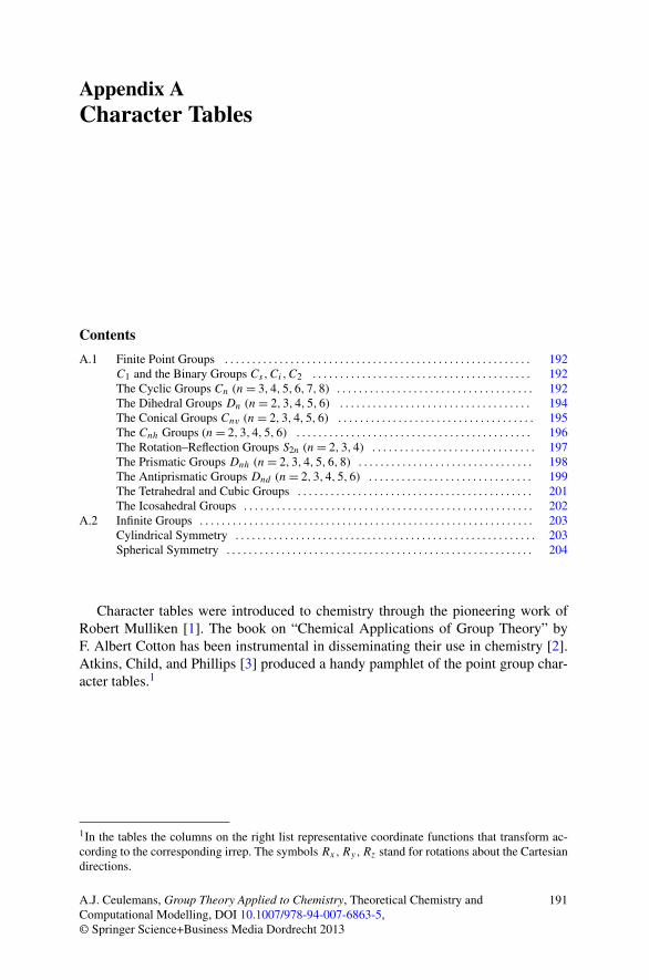
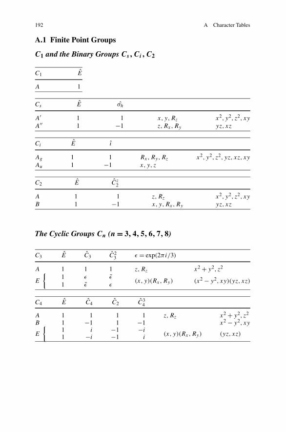
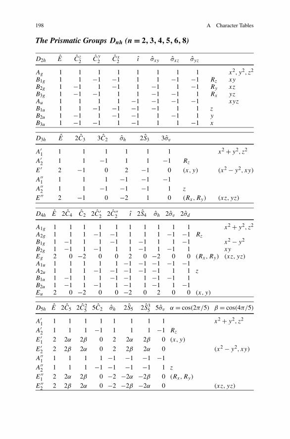
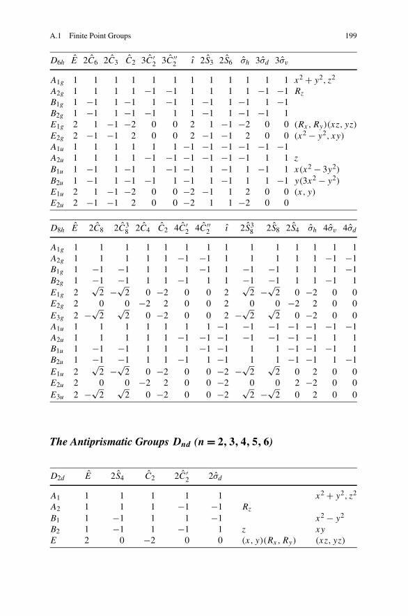
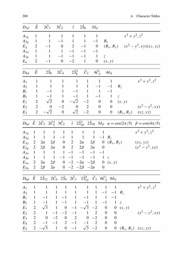
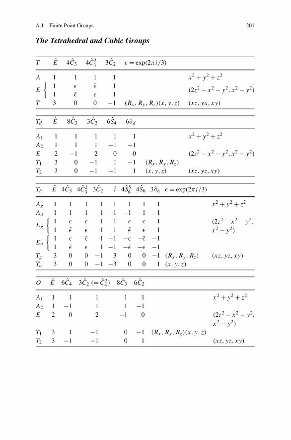
Character tables were introduced to chemistry through the pioneering work ofRobert Mulliken [1]. The book on “Chemical Applications of Group Theory” byF. Albert Cotton has been instrumental in disseminating their use in chemistry [2].Atkins, Child, and Phillips [3] produced a handy pamphlet of the point group char-acter tables.1
1In the tables the columns on the right list representative coordinate functions that transform ac-cording to the corresponding irrep. The symbols Rx,Ry,Rz stand for rotations about the Cartesiandirections.
A.J. Ceulemans, Group Theory Applied to Chemistry, Theoretical Chemistry andComputational Modelling, DOI 10.1007/978-94-007-6863-5,© Springer Science+Business Media Dordrecht 2013
191
192 A Character Tables
A.1 Finite Point Groups
C1 and the Binary Groups Cs,Ci,C2
C1 E
A 1
Cs E σh
A′ 1 1 x, y,Rz x2, y2, z2, xy
A′′ 1 −1 z,Rx,Ry yz, xz
Ci E ı
Ag 1 1 Rx,Ry,Rz x2, y2, z2, yz, xz, xy
Au 1 −1 x, y, z
C2 E Cz2
A 1 1 z,Rz x2, y2, z2, xy
B 1 −1 x, y,Rx,Ry yz, xz
The Cyclic Groups Cn (n = 3,4,5,6,7,8)
C3 E C3 C23 ε = exp(2πi/3)
A 1 1 1 z,Rz x2 + y2, z2
E
{1 ε ε
(x, y)(Rx,Ry) (x2 − y2, xy)(yz, xz)1 ε ε
C4 E C4 C2 C34
A 1 1 1 1 z,Rz x2 + y2, z2
B 1 −1 1 −1 x2 − y2, xy
E
{1 i −1 −i
(x, y)(Rx,Ry) (yz, xz)1 −i −1 i
A.1 Finite Point Groups 193
C5 E C5 C25 C3
5 C45 ε = exp(2πi/5)
A 1 1 1 1 1 z,Rz x2 + y2, z2
E1
{1 ε ε2 ε2 ε
(x, y)(Rx,Ry) (yz, xz)1 ε ε2 ε2 ε
E2
{1 ε2 ε ε ε2
(x2 − y2, xy)1 ε2 ε ε ε2
C6 E C6 C3 C2 C23 C5
6 ε = exp(2πi/6)
A 1 1 1 1 1 1 z,Rz x2 + y2, z2
B 1 −1 1 −1 1 −1
E1
{1 ε −ε −1 −ε ε
(x, y)(Rx,Ry) (yz, xz)1 ε −ε −1 −ε ε
E2
{1 −ε −ε 1 −ε −ε
(x2 − y2, xy)1 −ε −ε 1 −ε −ε
C7 E C7 C27 C3
7 C47 C5
7 C67 ε = exp(2πi/7)
A 1 1 1 1 1 1 1 z,Rz x2 + y2, z2
E1
{1 ε ε2 ε3 ε3 ε2 ε
(x, y)(Rx,Ry) (yz, xz)1 ε ε2 ε3 ε3 ε2 ε
E2
{1 ε2 ε3 ε ε ε3 ε2
(x2 − y2, xy)1 ε2 ε3 ε ε ε3 ε2
E3
{1 ε3 ε ε2 ε2 ε ε3 [x(x2 − 3y2),
y(3x2 − y2)]1 ε3 ε ε2 ε2 ε ε3
C8 E C8 C4 C2 C34 C3
8 C58 C7
8 ε = exp(2πi/8)
A 1 1 1 1 1 1 1 1 z,Rz x2 + y2, z2
B 1 −1 1 1 1 −1 −1 −1
E1
{1 ε i −1 −i −ε −ε ε
(x, y)(Rx,Ry) (yz, xz)1 ε −i −1 i −ε −ε ε
E2
{1 i −1 1 −1 −i i −i
(x2 − y2, xy)1 −i −1 1 −1 i −i i
E3
{1 −ε i −1 −i ε ε −ε [x(x2 − 3y2),
y(3x2 − y2)]1 −ε −i −1 i ε ε −ε
194 A Character Tables
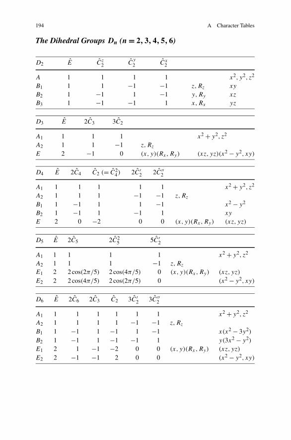
The Dihedral Groups Dn (n = 2,3,4,5,6)
D2 E Cz2 C
y
2 Cx2
A 1 1 1 1 x2, y2, z2
B1 1 1 −1 −1 z,Rz xy
B2 1 −1 1 −1 y,Ry xz
B3 1 −1 −1 1 x,Rx yz
D3 E 2C3 3C2
A1 1 1 1 x2 + y2, z2
A2 1 1 −1 z,Rz
E 2 −1 0 (x, y)(Rx,Ry) (xz, yz)(x2 − y2, xy)
D4 E 2C4 C2 (= C24) 2C′
2 2C′′2
A1 1 1 1 1 1 x2 + y2, z2
A2 1 1 1 −1 −1 z,Rz
B1 1 −1 1 1 −1 x2 − y2
B2 1 −1 1 −1 1 xy
E 2 0 −2 0 0 (x, y)(Rx,Ry) (xz, yz)
D5 E 2C5 2C25 5C′
2
A1 1 1 1 1 x2 + y2, z2
A2 1 1 1 −1 z,Rz
E1 2 2 cos(2π/5) 2 cos(4π/5) 0 (x, y)(Rx,Ry) (xz, yz)
E2 2 2 cos(4π/5) 2 cos(2π/5) 0 (x2 − y2, xy)
D6 E 2C6 2C3 C2 3C′2 3C′′
2
A1 1 1 1 1 1 1 x2 + y2, z2
A2 1 1 1 1 −1 −1 z,Rz
B1 1 −1 1 −1 1 −1 x(x2 − 3y2)
B2 1 −1 1 −1 −1 1 y(3x2 − y2)
E1 2 1 −1 −2 0 0 (x, y)(Rx,Ry) (xz, yz)
E2 2 −1 −1 2 0 0 (x2 − y2, xy)
A.1 Finite Point Groups 195
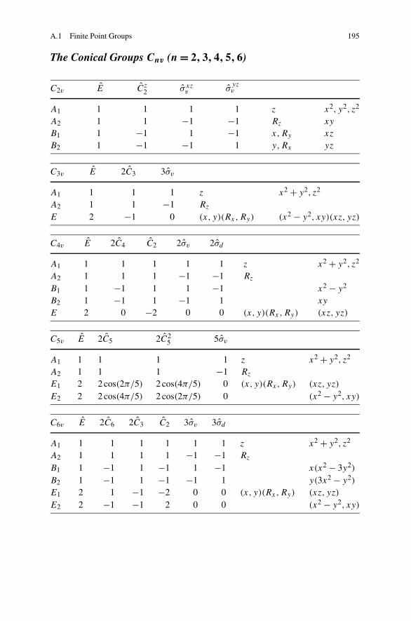
The Conical Groups Cnv (n = 2,3,4,5,6)
C2v E Cz2 σ xz
v σyzv
A1 1 1 1 1 z x2, y2, z2
A2 1 1 −1 −1 Rz xy
B1 1 −1 1 −1 x,Ry xz
B2 1 −1 −1 1 y,Rx yz
C3v E 2C3 3σv
A1 1 1 1 z x2 + y2, z2
A2 1 1 −1 Rz
E 2 −1 0 (x, y)(Rx,Ry) (x2 − y2, xy)(xz, yz)
C4v E 2C4 C2 2σv 2σd
A1 1 1 1 1 1 z x2 + y2, z2
A2 1 1 1 −1 −1 Rz
B1 1 −1 1 1 −1 x2 − y2
B2 1 −1 1 −1 1 xy
E 2 0 −2 0 0 (x, y)(Rx,Ry) (xz, yz)
C5v E 2C5 2C25 5σv
A1 1 1 1 1 z x2 + y2, z2
A2 1 1 1 −1 Rz
E1 2 2 cos(2π/5) 2 cos(4π/5) 0 (x, y)(Rx,Ry) (xz, yz)
E2 2 2 cos(4π/5) 2 cos(2π/5) 0 (x2 − y2, xy)
C6v E 2C6 2C3 C2 3σv 3σd
A1 1 1 1 1 1 1 z x2 + y2, z2
A2 1 1 1 1 −1 −1 Rz
B1 1 −1 1 −1 1 −1 x(x2 − 3y2)
B2 1 −1 1 −1 −1 1 y(3x2 − y2)
E1 2 1 −1 −2 0 0 (x, y)(Rx,Ry) (xz, yz)
E2 2 −1 −1 2 0 0 (x2 − y2, xy)
196 A Character Tables
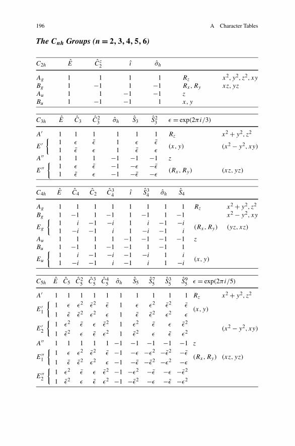
The Cnh Groups (n = 2,3,4,5,6)
C2h E Cz2 ı σh
Ag 1 1 1 1 Rz x2, y2, z2, xy
Bg 1 −1 1 −1 Rx,Ry xz, yz
Au 1 1 −1 −1 z
Bu 1 −1 −1 1 x, y
C3h E C3 C23 σh S3 S2
3 ε = exp(2πi/3)
A′ 1 1 1 1 1 1 Rz x2 + y2, z2
E′{
1 ε ε 1 ε ε(x, y) (x2 − y2, xy)
1 ε ε 1 ε ε
A′′ 1 1 1 −1 −1 −1 z
E′′{
1 ε ε −1 −ε −ε(Rx,Ry) (xz, yz)
1 ε ε −1 −ε −ε
C4h E C4 C2 C34 ı S3
4 σh S4
Ag 1 1 1 1 1 1 1 1 Rz x2 + y2, z2
Bg 1 −1 1 −1 1 −1 1 −1 x2 − y2, xy
Eg
{1 i −1 −i 1 i −1 −i
(Rx,Ry) (yz, xz)1 −i −1 i 1 −i −1 i
Au 1 1 1 1 −1 −1 −1 −1 z
Bu 1 −1 1 −1 −1 1 −1 1
Eu
{1 i −1 −i −1 −i 1 i
(x, y)1 −i −1 i −1 i 1 −i
C5h E C5 C25 C3
5 C45 σh S5 S7
5 S35 S9
5 ε = exp(2πi/5)
A′ 1 1 1 1 1 1 1 1 1 1 Rz x2 + y2, z2
E′1
{1 ε ε2 ε2 ε 1 ε ε2 ε2 ε
(x, y)1 ε ε2 ε2 ε 1 ε ε2 ε2 ε
E′2
{1 ε2 ε ε ε2 1 ε2 ε ε ε2
(x2 − y2, xy)1 ε2 ε ε ε2 1 ε2 ε ε ε2
A′′ 1 1 1 1 1 −1 −1 −1 −1 −1 z
E′′1
{1 ε ε2 ε2 ε −1 −ε −ε2 −ε2 −ε
(Rx,Ry) (xz, yz)1 ε ε2 ε2 ε −1 −ε −ε2 −ε2 −ε
E′′2
{1 ε2 ε ε ε2 −1 −ε2 −ε −ε −ε2
1 ε2 ε ε ε2 −1 −ε2 −ε −ε −ε2
A.1 Finite Point Groups 197
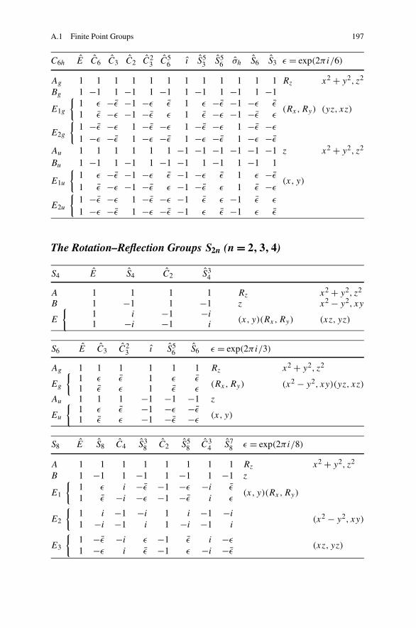
C6h E C6 C3 C2 C23 C5
6 ı S53 S5
6 σh S6 S3 ε = exp(2πi/6)
Ag 1 1 1 1 1 1 1 1 1 1 1 1 Rz x2 + y2, z2
Bg 1 −1 1 −1 1 −1 1 −1 1 −1 1 −1
E1g
{1 ε −ε −1 −ε ε 1 ε −ε −1 −ε ε
(Rx,Ry) (yz, xz)1 ε −ε −1 −ε ε 1 ε −ε −1 −ε ε
E2g
{1 −ε −ε 1 −ε −ε 1 −ε −ε 1 −ε −ε
1 −ε −ε 1 −ε −ε 1 −ε −ε 1 −ε −ε
Au 1 1 1 1 1 1 −1 −1 −1 −1 −1 −1 z x2 + y2, z2
Bu 1 −1 1 −1 1 −1 −1 1 −1 1 −1 1
E1u
{1 ε −ε −1 −ε ε −1 −ε ε 1 ε −ε
(x, y)1 ε −ε −1 −ε ε −1 −ε ε 1 ε −ε
E2u
{1 −ε −ε 1 −ε −ε −1 ε ε −1 ε ε
1 −ε −ε 1 −ε −ε −1 ε ε −1 ε ε
The Rotation–Reflection Groups S2n (n = 2,3,4)
S4 E S4 C2 S34
A 1 1 1 1 Rz x2 + y2, z2
B 1 −1 1 −1 z x2 − y2, xy
E
{1 i −1 −i
(x, y)(Rx,Ry) (xz, yz)1 −i −1 i
S6 E C3 C23 ı S5
6 S6 ε = exp(2πi/3)
Ag 1 1 1 1 1 1 Rz x2 + y2, z2
Eg
{1 ε ε 1 ε ε
(Rx,Ry) (x2 − y2, xy)(yz, xz)1 ε ε 1 ε εAu 1 1 1 −1 −1 −1 z
Eu
{1 ε ε −1 −ε −ε
(x, y)1 ε ε −1 −ε −ε
S8 E S8 C4 S38 C2 S5
8 C34 S7
8 ε = exp(2πi/8)
A 1 1 1 1 1 1 1 1 Rz x2 + y2, z2
B 1 −1 1 −1 1 −1 1 −1 z
E1
{1 ε i −ε −1 −ε −i ε
(x, y)(Rx,Ry)1 ε −i −ε −1 −ε i ε
E2
{1 i −1 −i 1 i −1 −i
(x2 − y2, xy)1 −i −1 i 1 −i −1 i
E3
{1 −ε −i ε −1 ε i −ε
(xz, yz)1 −ε i ε −1 ε −i −ε
198 A Character Tables
The Prismatic Groups Dnh (n = 2,3,4,5,6,8)
D2h E Cz2 C
y
2 Cx2 ı σxy σxz σyz
Ag 1 1 1 1 1 1 1 1 x2, y2, z2
B1g 1 1 −1 −1 1 1 −1 −1 Rz xyB2g 1 −1 1 −1 1 −1 1 −1 Ry xzB3g 1 −1 −1 1 1 −1 −1 1 Rx yzAu 1 1 1 1 −1 −1 −1 −1 xyzB1u 1 1 −1 −1 −1 −1 1 1 zB2u 1 −1 1 −1 −1 1 −1 1 yB3u 1 −1 −1 1 −1 1 1 −1 x
D3h E 2C3 3C2 σh 2S3 3σv
A′1 1 1 1 1 1 1 x2 + y2, z2
A′2 1 1 −1 1 1 −1 Rz
E′ 2 −1 0 2 −1 0 (x, y) (x2 − y2, xy)
A′′1 1 1 1 −1 −1 −1
A′′2 1 1 −1 −1 −1 1 z
E′′ 2 −1 0 −2 1 0 (Rx,Ry) (xz, yz)
D4h E 2C4 C2 2C′2 2C′′
2 ı 2S4 σh 2σv 2σd
A1g 1 1 1 1 1 1 1 1 1 1 x2 + y2, z2
A2g 1 1 1 −1 −1 1 1 1 −1 −1 Rz
B1g 1 −1 1 1 −1 1 −1 1 1 −1 x2 − y2
B2g 1 −1 1 −1 1 1 −1 1 −1 1 xyEg 2 0 −2 0 0 2 0 −2 0 0 (Rx,Ry) (xz, yz)A1u 1 1 1 1 1 −1 −1 −1 −1 −1A2u 1 1 1 −1 −1 −1 −1 −1 1 1 zB1u 1 −1 1 1 −1 −1 1 −1 −1 1B2u 1 −1 1 −1 1 −1 1 −1 1 −1Eu 2 0 −2 0 0 −2 0 2 0 0 (x, y)
D5h E 2C5 2C25 5C2 σh 2S5 2S3
5 5σv α = cos(2π/5) β = cos(4π/5)
A′1 1 1 1 1 1 1 1 1 x2 + y2, z2
A′2 1 1 1 −1 1 1 1 −1 Rz
E′1 2 2α 2β 0 2 2α 2β 0 (x, y)
E′2 2 2β 2α 0 2 2β 2α 0 (x2 − y2, xy)
A′′1 1 1 1 1 −1 −1 −1 −1
A′′2 1 1 1 −1 −1 −1 −1 1 z
E′′1 2 2α 2β 0 −2 −2α −2β 0 (Rx,Ry)
E′′2 2 2β 2α 0 −2 −2β −2α 0 (xz, yz)
A.1 Finite Point Groups 199
D6h E 2C6 2C3 C2 3C′2 3C′′
2 ı 2S3 2S6 σh 3σd 3σv
A1g 1 1 1 1 1 1 1 1 1 1 1 1 x2 + y2, z2
A2g 1 1 1 1 −1 −1 1 1 1 1 −1 −1 Rz
B1g 1 −1 1 −1 1 −1 1 −1 1 −1 1 −1B2g 1 −1 1 −1 −1 1 1 −1 1 −1 −1 1E1g 2 1 −1 −2 0 0 2 1 −1 −2 0 0 (Rx,Ry)(xz, yz)
E2g 2 −1 −1 2 0 0 2 −1 −1 2 0 0 (x2 − y2, xy)
A1u 1 1 1 1 1 1 −1 −1 −1 −1 −1 −1A2u 1 1 1 1 −1 −1 −1 −1 −1 −1 1 1 z
B1u 1 −1 1 −1 1 −1 −1 1 −1 1 −1 1 x(x2 − 3y2)
B2u 1 −1 1 −1 −1 1 −1 1 −1 1 1 −1 y(3x2 − y2)
E1u 2 1 −1 −2 0 0 −2 −1 1 2 0 0 (x, y)
E2u 2 −1 −1 2 0 0 −2 1 1 −2 0 0
D8h E 2C8 2C38 2C4 C2 4C′
2 4C′′2 ı 2S3
8 2S8 2S4 σh 4σv 4σd
A1g 1 1 1 1 1 1 1 1 1 1 1 1 1 1A2g 1 1 1 1 1 −1 −1 1 1 1 1 1 −1 −1B1g 1 −1 −1 1 1 1 −1 1 −1 −1 1 1 1 −1B2g 1 −1 −1 1 1 −1 1 1 −1 −1 1 1 −1 1E1g 2
√2 −√
2 0 −2 0 0 2√
2 −√2 0 −2 0 0
E2g 2 0 0 −2 2 0 0 2 0 0 −2 2 0 0E3g 2 −√
2√
2 0 −2 0 0 2 −√2
√2 0 −2 0 0
A1u 1 1 1 1 1 1 1 −1 −1 −1 −1 −1 −1 −1A2u 1 1 1 1 1 −1 −1 −1 −1 −1 −1 −1 1 1B1u 1 −1 −1 1 1 1 −1 −1 1 1 −1 −1 −1 1B2u 1 −1 −1 1 1 −1 1 −1 1 1 −1 −1 1 −1E1u 2
√2 −√
2 0 −2 0 0 −2 −√2
√2 0 2 0 0
E2u 2 0 0 −2 2 0 0 −2 0 0 2 −2 0 0E3u 2 −√
2√
2 0 −2 0 0 −2√
2 −√2 0 2 0 0
The Antiprismatic Groups Dnd (n = 2,3,4,5,6)
D2d E 2S4 C2 2C′2 2σd
A1 1 1 1 1 1 x2 + y2, z2
A2 1 1 1 −1 −1 Rz
B1 1 −1 1 1 −1 x2 − y2
B2 1 −1 1 −1 1 z xy
E 2 0 −2 0 0 (x, y)(Rx,Ry) (xz, yz)
200 A Character Tables
D3d E 2C3 3C2 ı 2S6 3σd
A1g 1 1 1 1 1 1 x2 + y2, z2
A2g 1 1 −1 1 1 −1 Rz
Eg 2 −1 0 2 −1 0 (Rx,Ry) (x2 − y2, xy)(xz, yz)
A1u 1 1 1 −1 −1 −1A2u 1 1 −1 −1 −1 1 z
Eu 2 −1 0 −2 1 0 (x, y)
D4d E 2S8 2C4 2S38 C2 4C′
2 4σd
A1 1 1 1 1 1 1 1 x2 + y2, z2
A2 1 1 1 1 1 −1 −1 Rz
B1 1 −1 1 −1 1 1 −1B2 1 −1 1 −1 1 −1 1 z
E1 2√
2 0 −√2 −2 0 0 (x, y)
E2 2 0 −2 0 2 0 0 (x2 − y2, xy)
E3 2 −√2 0
√2 −2 0 0 (Rx,Ry) (xz, yz)
D5d E 2C5 2C25 5C2 ı 2S3
10 2S10 5σd α = cos(2π/5) β = cos(4π/5)
A1g 1 1 1 1 1 1 1 1 x2 + y2, z2
A2g 1 1 1 −1 1 1 1 −1 Rz
E1g 2 2α 2β 0 2 2α 2β 0 (Rx,Ry) (xz, yz)
E2g 2 2β 2α 0 2 2β 2α 0 (x2 − y2, xy)
A1u 1 1 1 1 −1 −1 −1 −1A2u 1 1 1 −1 −1 −1 −1 1 z
E1u 2 2α 2β 0 −2 −2α −2β 0 (x, y)
E2u 2 2β 2α 0 −2 −2β −2α 0
D6d E 2S12 2C6 2S4 2C3 2S512 C2 6C′
2 6σd
A1 1 1 1 1 1 1 1 1 1 x2 + y2, z2
A2 1 1 1 1 1 1 1 −1 −1 Rz
B1 1 −1 1 −1 1 −1 1 1 −1B2 1 −1 1 −1 1 −1 1 −1 1 z
E1 2√
3 1 0 −1 −√3 −2 0 0 (x, y)
E2 2 1 −1 −2 −1 1 2 0 0 (x2 − y2, xy)
E3 2 0 −2 0 2 0 −2 0 0E4 2 −1 −1 2 −1 −1 2 0 0E5 2 −√
3 1 0 −1√
3 −2 0 0 (Rx,Ry) (xz, yz)
A.1 Finite Point Groups 201
The Tetrahedral and Cubic Groups
T E 4C3 4C23 3C2 ε = exp(2πi/3)
A 1 1 1 1 x2 + y2 + z2
E
{1 ε ε 1
(2z2 − x2 − y2, x2 − y2)1 ε ε 1
T 3 0 0 −1 (Rx,Ry,Rz)(x, y, z) (xz, yx, xy)
Td E 8C3 3C2 6S4 6σd
A1 1 1 1 1 1 x2 + y2 + z2
A2 1 1 1 −1 −1E 2 −1 2 0 0 (2z2 − x2 − y2, x2 − y2)
T1 3 0 −1 1 −1 (Rx,Ry,Rz)
T2 3 0 −1 −1 1 (x, y, z) (xz, yz, xy)
Th E 4C3 4C23 3C2 ı 4S5
6 4S6 3σh ε = exp(2πi/3)
Ag 1 1 1 1 1 1 1 1 x2 + y2 + z2
Au 1 1 1 1 −1 −1 −1 −1
Eg
{1 ε ε 1 1 ε ε 1 (2z2 − x2 − y2,
x2 − y2)1 ε ε 1 1 ε ε 1
Eu
{1 ε ε 1 −1 −ε −ε −11 ε ε 1 −1 −ε −ε −1
Tg 3 0 0 −1 3 0 0 −1 (Rx,Ry,Rz) (xz, yz, xy)
Tu 3 0 0 −1 −3 0 0 1 (x, y, z)
O E 6C4 3C2 (= C24) 8C3 6C2
A1 1 1 1 1 1 x2 + y2 + z2
A2 1 −1 1 1 −1E 2 0 2 −1 0 (2z2 − x2 − y2,
x2 − y2)
T1 3 1 −1 0 −1 (Rx,Ry,Rz)(x, y, z)
T2 3 −1 −1 0 1 (xz, yz, xy)
202 A Character Tables
Oh E 8C3 6C2 6C4 3C2 ı 6S4 8S6 3σh 6σd
A1g 1 1 1 1 1 1 1 1 1 1 x2 + y2 + z2
A2g 1 1 −1 −1 1 1 −1 1 1 −1Eg 2 −1 0 0 2 2 0 −1 2 0 (2z2 − x2 − y2,
x2 − y2)
T1g 3 0 −1 1 −1 3 1 0 −1 −1 (Rx,Ry,Rz)
T2g 3 0 1 −1 −1 3 −1 0 −1 1 (xz, yz, xy)
A1u 1 1 1 1 1 −1 −1 −1 −1 −1A2u 1 1 −1 −1 1 −1 1 −1 −1 1Eu 2 −1 0 0 2 −2 0 1 −2 0T1u 3 0 −1 1 −1 −3 −1 0 1 1 (x, y, z)
T2u 3 0 1 −1 −1 −3 1 0 1 −1
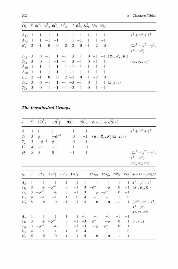
The Icosahedral Groups
I E 12C5 12C25 20C3 15C2 φ = (1 + √
5)/2
A 1 1 1 1 1 x2 + y2 + z2
T1 3 φ −φ−1 0 −1 (Rx,Ry,Rz)(x, y, z)
T2 3 −φ−1 φ 0 −1G 4 −1 −1 1 0H 5 0 0 −1 1 (2z2 − x2 − y2,
x2 − y2,
(xz, yz, xy)
Ih E 12C5 12C25 20C3 15C2 ı 12S10 12S3
10 20S6 15σ φ = (1 + √5)/2
Ag 1 1 1 1 1 1 1 1 1 1 x2 + y2 + z2
T1g 3 φ −φ−1 0 −1 3 −φ−1 φ 0 −1 (Rx,Ry,Rz)
T2g 3 −φ−1 φ 0 −1 3 φ −φ−1 0 −1Gg 4 −1 −1 1 0 4 −1 −1 1 0Hg 5 0 0 −1 1 5 0 0 −1 1 (2z2 − x2 − y2,
x2 − y2,
xz, yz, xy)
Au 1 1 1 1 1 −1 −1 −1 −1 −1T1u 3 φ −φ−1 0 −1 −3 φ−1 −φ 0 1 (x, y, z)
T2u 3 −φ−1 φ 0 −1 −3 −φ φ−1 0 1Gu 4 −1 −1 1 0 −4 1 1 −1 0Hu 5 0 0 −1 1 −5 0 0 1 −1
A.2 Infinite Groups 203
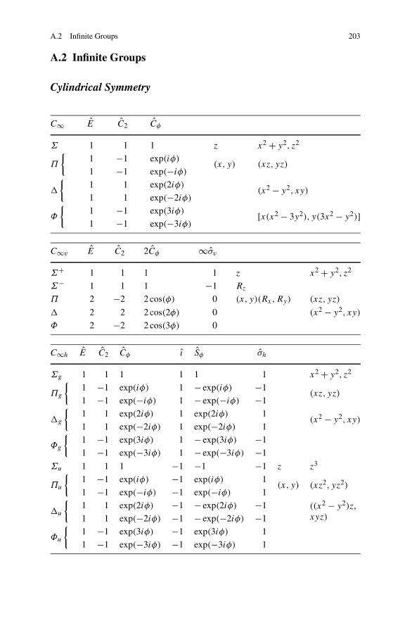
A.2 Infinite Groups
Cylindrical Symmetry
C∞ E C2 Cφ
Σ 1 1 1 z x2 + y2, z2
Π
{1 −1 exp(iφ)
(x, y) (xz, yz)1 −1 exp(−iφ)
{1 1 exp(2iφ)
(x2 − y2, xy)1 1 exp(−2iφ)
Φ
{1 −1 exp(3iφ) [x(x2 − 3y2), y(3x2 − y2)]1 −1 exp(−3iφ)
C∞v E C2 2Cφ ∞σv
Σ+ 1 1 1 1 z x2 + y2, z2
Σ− 1 1 1 −1 Rz
Π 2 −2 2 cos(φ) 0 (x, y)(Rx,Ry) (xz, yz)
2 2 2 cos(2φ) 0 (x2 − y2, xy)
Φ 2 −2 2 cos(3φ) 0
C∞h E C2 Cφ ı Sφ σh
Σg 1 1 1 1 1 1 x2 + y2, z2
Πg
{1 −1 exp(iφ) 1 − exp(iφ) −1
(xz, yz)1 −1 exp(−iφ) 1 − exp(−iφ) −1
g
{1 1 exp(2iφ) 1 exp(2iφ) 1
(x2 − y2, xy)1 1 exp(−2iφ) 1 exp(−2iφ) 1
Φg
{1 −1 exp(3iφ) 1 − exp(3iφ) −1
1 −1 exp(−3iφ) 1 − exp(−3iφ) −1
Σu 1 1 1 −1 −1 −1 z z3
Πu
{1 −1 exp(iφ) −1 exp(iφ) 1
(x, y) (xz2, yz2)1 −1 exp(−iφ) −1 exp(−iφ) 1
u
{1 1 exp(2iφ) −1 − exp(2iφ) −1 ((x2 − y2)z,
xyz)1 1 exp(−2iφ) −1 − exp(−2iφ) −1
Φu
{1 −1 exp(3iφ) −1 exp(3iφ) 1
1 −1 exp(−3iφ) −1 exp(−3iφ) 1
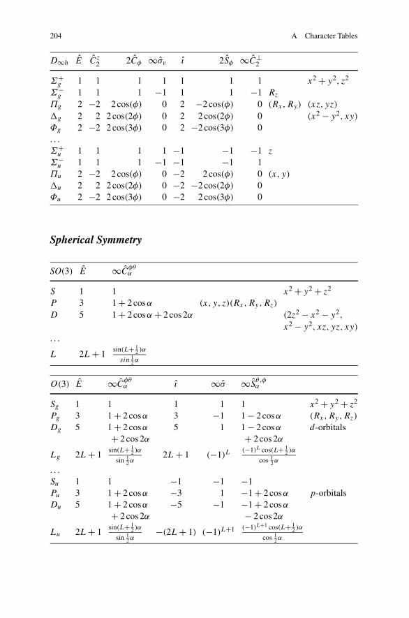
204 A Character Tables
D∞h E Cz2 2Cφ ∞σv ı 2Sφ ∞C⊥
2
Σ+g 1 1 1 1 1 1 1 x2 + y2, z2
Σ−g 1 1 1 −1 1 1 −1 Rz
Πg 2 −2 2 cos(φ) 0 2 −2 cos(φ) 0 (Rx,Ry) (xz, yz)
g 2 2 2 cos(2φ) 0 2 2 cos(2φ) 0 (x2 − y2, xy)
Φg 2 −2 2 cos(3φ) 0 2 −2 cos(3φ) 0. . .Σ+
u 1 1 1 1 −1 −1 −1 z
Σ−u 1 1 1 −1 −1 −1 1
Πu 2 −2 2 cos(φ) 0 −2 2 cos(φ) 0 (x, y)
u 2 2 2 cos(2φ) 0 −2 −2 cos(2φ) 0Φu 2 −2 2 cos(3φ) 0 −2 2 cos(3φ) 0
Spherical Symmetry
SO(3) E ∞Cφθα
S 1 1 x2 + y2 + z2
P 3 1 + 2 cosα (x, y, z)(Rx,Ry,Rz)
D 5 1 + 2 cosα + 2 cos 2α (2z2 − x2 − y2,
x2 − y2, xz, yz, xy)
. . .
L 2L + 1sin(L+ 1
2 )α
sin 12 α
O(3) E ∞Cφθα ı ∞σ ∞S
θ,φα
Sg 1 1 1 1 1 x2 + y2 + z2
Pg 3 1 + 2 cosα 3 −1 1 − 2 cosα (Rx,Ry,Rz)
Dg 5 1 + 2 cosα 5 1 1 − 2 cosα d-orbitals+ 2 cos 2α + 2 cos 2α
Lg 2L + 1sin(L+ 1
2 )α
sin 12 α
2L + 1 (−1)L(−1)L cos(L+ 1
2 )α
cos 12 α
. . .Su 1 1 −1 −1 −1Pu 3 1 + 2 cosα −3 1 −1 + 2 cosα p-orbitalsDu 5 1 + 2 cosα −5 −1 −1 + 2 cosα
+ 2 cos 2α − 2 cos 2α
Lu 2L + 1sin(L+ 1
2 )α
sin 12 α
−(2L + 1) (−1)L+1 (−1)L+1 cos(L+ 12 )α
cos 12 α
Appendix BSymmetry Breaking by Uniform Linear Electricand Magnetic Fields
Contents
B.1 Spherical Groups . . . . . . . . . . . . . . . . . . . . . . . . . . . . . . . . . . . . . . . . . . . . . . . . . . . . . . . . . . . 205B.2 Binary and Cylindrical Groups . . . . . . . . . . . . . . . . . . . . . . . . . . . . . . . . . . . . . . . . . . . . . . 205
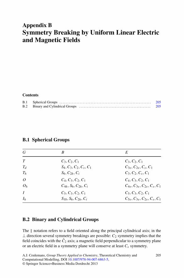
B.1 Spherical Groups
G B E
T C3,C2,C1 C3,C2,C1
Td S4,C3,C2,Cs,C1 C3v,C2v,Cs,C1
Th S6,C2h,Ci C3,C2,Cs,C1
O C4,C3,C2,C1 C4,C3,C2,C1
Oh C4h, S6,C2h,Ci C4v,C3v,C2v,Cs,C1
I C5,C3,C2,C1 C5,C3,C2,C1
Ih S10, S6,C2h,Ci C5v,C3v,C2v,Cs,C1
B.2 Binary and Cylindrical Groups
The ‖ notation refers to a field oriented along the principal cylindrical axis; in the⊥ direction several symmetry breakings are possible: C2 symmetry implies that thefield coincides with the C2 axis; a magnetic field perpendicular to a symmetry planeor an electric field in a symmetry plane will conserve at least Cs symmetry.
A.J. Ceulemans, Group Theory Applied to Chemistry, Theoretical Chemistry andComputational Modelling, DOI 10.1007/978-94-007-6863-5,© Springer Science+Business Media Dordrecht 2013
205
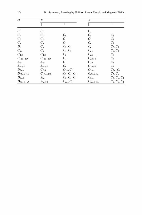
206 B Symmetry Breaking by Uniform Linear Electric and Magnetic Fields
G B E
‖ ⊥ ‖ ⊥Ci Ci C1Cs C1 Cs Cs C1C2 C2 C1 C2 C1Cn Cn C1 Cn C1Dn Cn C2,C1 Cn C2,C1Cnv Cn Cs,C1 Cnv Cs,C1C2nh C2nh Ci C2n Cs
C(2n+1)h C(2n+1)h C1 C2n+1 Cs
S4n S4n C1 C2n C1S4n+2 S4n+2 Ci C2n+1 C1D2nh C2nh C2h,Ci C2nv C2v,Cs
D(2n+1)h C(2n+1)h C2,Cs,C1 C(2n+1)v C2,Cs
D2nd S4n C2,Cs,C1 C2nv C2,Cs,C1D(2n+1)d S4n+2 C2h,Ci C(2n+1)v C2,Cs,C1
Appendix CSubduction and Induction
Contents
C.1 Subduction G ↓ H . . . . . . . . . . . . . . . . . . . . . . . . . . . . . . . . . . . . . . . . . . . . . . . . . . . . . . . . . 207C.2 Induction: H ↑ G . . . . . . . . . . . . . . . . . . . . . . . . . . . . . . . . . . . . . . . . . . . . . . . . . . . . . . . . . . 211
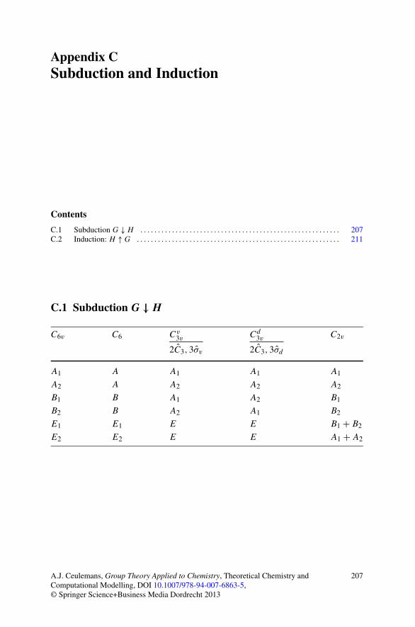
C.1 Subduction G ↓ H
C6v C6 Cv3v Cd
3v C2v
2C3,3σv 2C3,3σd
A1 A A1 A1 A1
A2 A A2 A2 A2
B1 B A1 A2 B1
B2 B A2 A1 B2
E1 E1 E E B1 + B2
E2 E2 E E A1 + A2
A.J. Ceulemans, Group Theory Applied to Chemistry, Theoretical Chemistry andComputational Modelling, DOI 10.1007/978-94-007-6863-5,© Springer Science+Business Media Dordrecht 2013
207
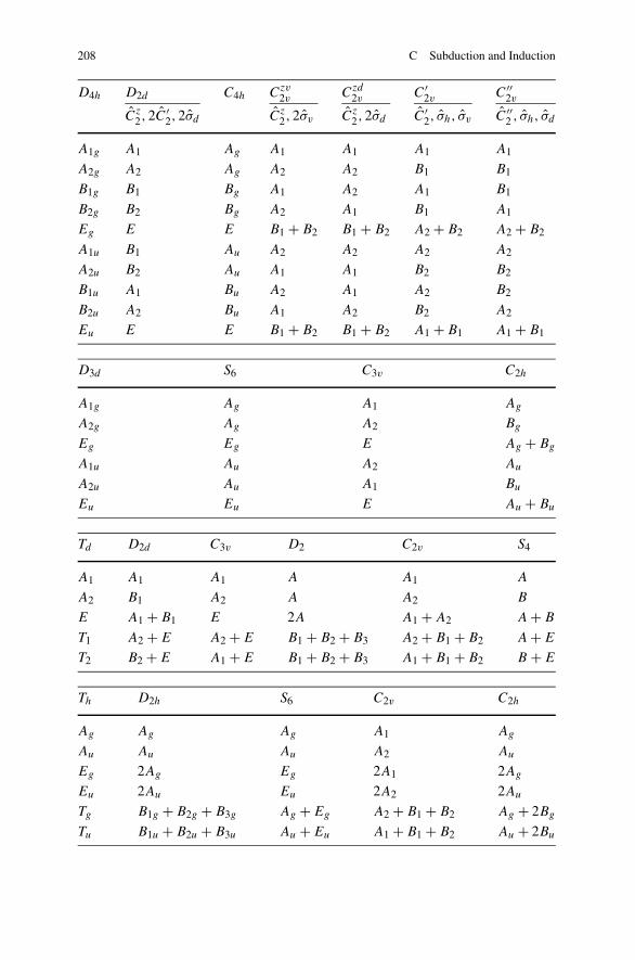
208 C Subduction and Induction
D4h D2d C4h Czv2v Czd
2v C′2v C′′
2v
Cz2,2C′
2,2σd Cz2,2σv Cz
2,2σd C′2, σh, σv C′′
2 , σh, σd
A1g A1 Ag A1 A1 A1 A1
A2g A2 Ag A2 A2 B1 B1
B1g B1 Bg A1 A2 A1 B1
B2g B2 Bg A2 A1 B1 A1
Eg E E B1 + B2 B1 + B2 A2 + B2 A2 + B2
A1u B1 Au A2 A2 A2 A2
A2u B2 Au A1 A1 B2 B2
B1u A1 Bu A2 A1 A2 B2
B2u A2 Bu A1 A2 B2 A2
Eu E E B1 + B2 B1 + B2 A1 + B1 A1 + B1
D3d S6 C3v C2h
A1g Ag A1 Ag
A2g Ag A2 Bg
Eg Eg E Ag + Bg
A1u Au A2 Au
A2u Au A1 Bu
Eu Eu E Au + Bu
Td D2d C3v D2 C2v S4
A1 A1 A1 A A1 A
A2 B1 A2 A A2 B
E A1 + B1 E 2A A1 + A2 A + B
T1 A2 + E A2 + E B1 + B2 + B3 A2 + B1 + B2 A + E
T2 B2 + E A1 + E B1 + B2 + B3 A1 + B1 + B2 B + E
Th D2h S6 C2v C2h
Ag Ag Ag A1 Ag
Au Au Au A2 Au
Eg 2Ag Eg 2A1 2Ag
Eu 2Au Eu 2A2 2Au
Tg B1g + B2g + B3g Ag + Eg A2 + B1 + B2 Ag + 2Bg
Tu B1u + B2u + B3u Au + Eu A1 + B1 + B2 Au + 2Bu
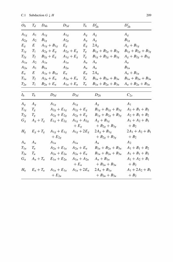
C.1 Subduction G ↓ H 209
Oh Td D4h D3d Th Dz2h D′
2h
A1g A1 A1g A1g Ag Ag Ag
A2g A2 B1g A2g Ag Ag B1g
Eg E A1g + B1g Eg Eg 2Ag Ag + B1g
T1g T1 A2g + Eg A2g + Eg Tg B1g + B2g + B3g B1g + B2g + B3g
T2g T2 B2g + Eg A1g + Eg Tg B1g + B2g + B3g Ag + B2g + B3g
A1u A2 A1u A1u Au Au Au
A2u A1 B1u A2u Au Au B1u
Eu E A1u + B1u Eu Eu 2Au Au + B1u
T1u T2 A2u + Eu A2u + Eu Tu B1u + B2u + B3u B1u + B2u + B3u
T2u T1 B2u + Eu A1u + Eu Tu B1u + B2u + B3u Au + B2u + B3u
Ih Th D5d D3d D2h C2v
Ag Ag A1g A1g Ag A1
T1g Tg A2g + E1g A2g + Eg B1g + B2g + B3g A2 + B1 + B2
T2g Tg A2g + E2g A2g + Eg B1g + B2g + B3g A2 + B1 + B2
Gg Ag + Tg E1g + E2g A1g + A2g Ag + B1g A1 + A2 + B1
+ Eg + B2g + B3g + B2
Hg Eg + Tg A1g + E1g A1g + 2Eg 2Ag + B1g 2A1 + A2 + B1
+ E2g + B2g + B3g + B2
Au Au A1u A1u Au A2
T1u Tu A2u + E1u A2u + Eu B1u + B2u + B3u A1 + B1 + B2
T2u Tu A2u + E2u A2u + Eu B1u + B2u + B3u A1 + B1 + B2
Gu Au + Tu E1u + E2u A1u + A2u Au + B1u A1 + A2 + B1
+ Eu + B2u + B3u + B2
Hu Eu + Tu A1u + E1u A1u + 2Eu 2Au + B1u A1 + 2A2 + B1
+ E2u + B2u + B3u + B2
210 C Subduction and Induction
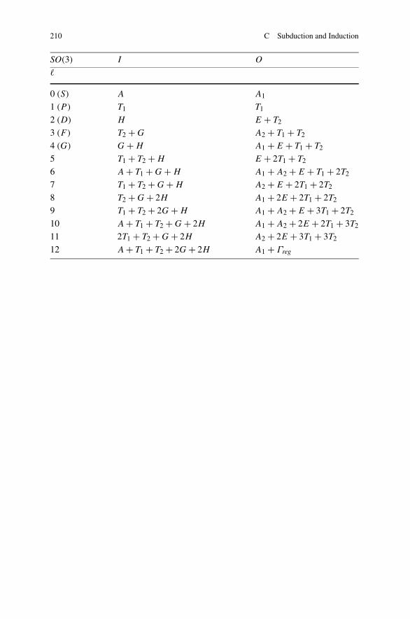
SO(3) I O
0 (S) A A1
1 (P ) T1 T1
2 (D) H E + T2
3 (F ) T2 + G A2 + T1 + T2
4 (G) G + H A1 + E + T1 + T2
5 T1 + T2 + H E + 2T1 + T2
6 A + T1 + G + H A1 + A2 + E + T1 + 2T2
7 T1 + T2 + G + H A2 + E + 2T1 + 2T2
8 T2 + G + 2H A1 + 2E + 2T1 + 2T2
9 T1 + T2 + 2G + H A1 + A2 + E + 3T1 + 2T2
10 A + T1 + T2 + G + 2H A1 + A2 + 2E + 2T1 + 3T2
11 2T1 + T2 + G + 2H A2 + 2E + 3T1 + 3T2
12 A + T1 + T2 + 2G + 2H A1 + Γreg
C.2 Induction: H ↑ G 211
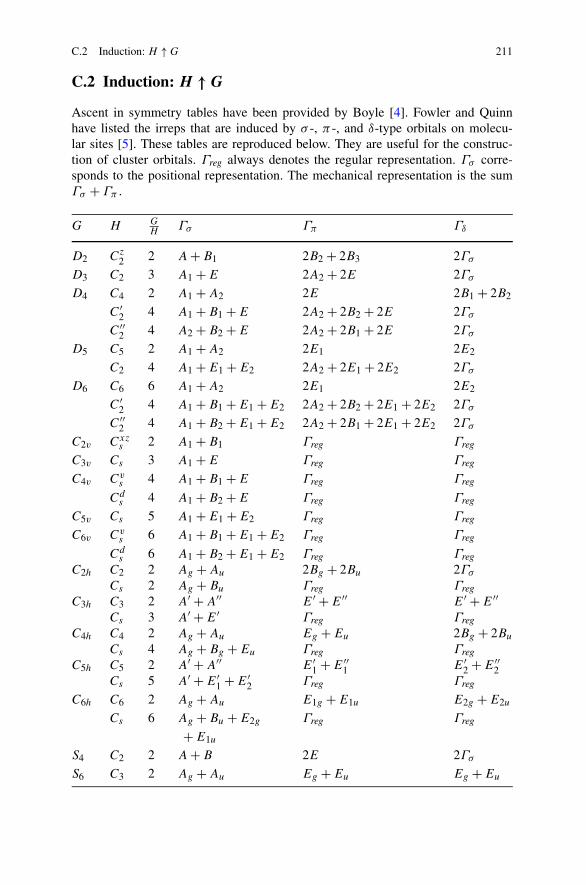
C.2 Induction: H ↑ G
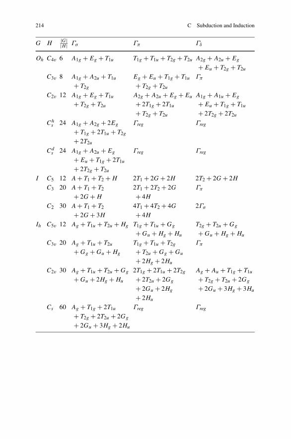
Ascent in symmetry tables have been provided by Boyle [4]. Fowler and Quinnhave listed the irreps that are induced by σ -, π -, and δ-type orbitals on molecu-lar sites [5]. These tables are reproduced below. They are useful for the construc-tion of cluster orbitals. Γreg always denotes the regular representation. Γσ corre-sponds to the positional representation. The mechanical representation is the sumΓσ + Γπ .
G H GH
Γσ Γπ Γδ
D2 Cz2 2 A + B1 2B2 + 2B3 2Γσ
D3 C2 3 A1 + E 2A2 + 2E 2Γσ
D4 C4 2 A1 + A2 2E 2B1 + 2B2
C′2 4 A1 + B1 + E 2A2 + 2B2 + 2E 2Γσ
C′′2 4 A2 + B2 + E 2A2 + 2B1 + 2E 2Γσ
D5 C5 2 A1 + A2 2E1 2E2
C2 4 A1 + E1 + E2 2A2 + 2E1 + 2E2 2Γσ
D6 C6 6 A1 + A2 2E1 2E2
C′2 4 A1 + B1 + E1 + E2 2A2 + 2B2 + 2E1 + 2E2 2Γσ
C′′2 4 A1 + B2 + E1 + E2 2A2 + 2B1 + 2E1 + 2E2 2Γσ
C2v Cxzs 2 A1 + B1 Γreg Γreg
C3v Cs 3 A1 + E Γreg Γreg
C4v Cvs 4 A1 + B1 + E Γreg Γreg
Cds 4 A1 + B2 + E Γreg Γreg
C5v Cs 5 A1 + E1 + E2 Γreg Γreg
C6v Cvs 6 A1 + B1 + E1 + E2 Γreg Γreg
Cds 6 A1 + B2 + E1 + E2 Γreg Γreg
C2h C2 2 Ag + Au 2Bg + 2Bu 2Γσ
Cs 2 Ag + Bu Γreg Γreg
C3h C3 2 A′ + A′′ E′ + E′′ E′ + E′′Cs 3 A′ + E′ Γreg Γreg
C4h C4 2 Ag + Au Eg + Eu 2Bg + 2Bu
Cs 4 Ag + Bg + Eu Γreg Γreg
C5h C5 2 A′ + A′′ E′1 + E′′
1 E′2 + E′′
2Cs 5 A′ + E′
1 + E′2 Γreg Γreg
C6h C6 2 Ag + Au E1g + E1u E2g + E2u
Cs 6 Ag + Bu + E2g Γreg Γreg
+ E1u
S4 C2 2 A + B 2E 2Γσ
S6 C3 2 Ag + Au Eg + Eu Eg + Eu
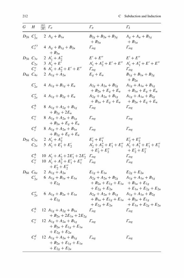
212 C Subduction and Induction
G H|G||H | Γσ Γπ Γδ
D2h Cz2v 2 Ag + B1u B2g + B2u + B3g Ag + Au + B1g
+ B3u + B1u
Cxys 4 Ag + B1g + B2u Γreg Γreg
+ B3u
D3h C3v 2 A′1 + A′′
2 E′ + E′′ E′ + E′′C2v 3 A′
1 + E′ A′1 + A′′
2 + E′ + E′′ A′1 + A′′
1 + E′ + E′′Cv
s 6 A′1 + A′′
2 + E′ + E′′ Γreg Γreg
D4h C4v 2 A1g + A2u Eg + Eu B1g + B1u + B2g
+ B2u
C′2v 4 A1g + B1g + Eu A2g + A2u + B2g A1g + A1u + B1g
+ B2u + Eg + Eu + B1u + Eg + Eu
C′′2v 4 A1g + B2g + Eu A2g + A2u + B1g A1g + A1u + B2g
+ B1u + Eg + Eu + B2u + Eg + Eu
Chs 8 A1g + A2g + B1g Γreg Γreg
+ B2g + 2Eu
Cvs 8 A1g + A2u + B1g Γreg Γreg
+ B2u + Eg + Eu
Cds 8 A1g + A2u + B1u Γreg Γreg
+ B2g + Eg + Eu
D5h C5v 2 A′1 + A′′
2 E′1 + E′′
1 E′2 + E′′
2C2v 5 A′
1 + E′1 + E′
2 A′2 + A′′
2 + E′1 + E′′
1 A′1 + A′′
1 + E′1 + E′′
1+ E′
2 + E′′2 + E′
2 + E′′2
Chs 10 A′
1 + A′2 + 2E′
1 + 2E′2 Γreg Γreg
Cvs 10 A′
1 + A′′2 + E′
1 + E′′1 Γreg Γreg
+ E′2 + E′′
2D6h C6v 2 A1g + A2u E1g + E1u E2g + E2u
C′2v 6 A1g + B1u + E1u A2g + A2u + B2g A1g + A1u + B1g
+ E2g + B2u + E1g + E1u + B1u + E1g
+ E2g + E2u + E1u + E2g + E2u
C′′2v 6 A1g + B2u + E1u A2g + A2u + B1g A1g + A1u + B2g
+ E2g + B1u + E1g + E1u + B2u + E1g
+ E2g + E2u + E1u + E2g + E2u
Chs 12 A1g + A2g + B1u Γreg Γreg
+ B2u + 2E1u + 2E2g
Cvs 12 A1g + A2u + B1g Γreg Γreg
+ B2u + E1g + E1u
+ E2g + E2u
Cds 12 A1g + A2u + B1g Γreg Γreg
+ B2u + E1g + E1u
+ E2g + E2u
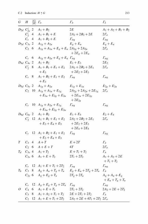
C.2 Induction: H ↑ G 213
G H|G||H | Γσ Γπ Γδ
D2d Cz2v 2 A1 + B2 2E A1 + A2 + B1 + B2
C′2 4 A1 + B1 + E 2A2 + 2B2 + 2E 2Γσ
Cs 4 A1 + B2 + E Γreg Γreg
D3d C3v 2 A1g + A2u Eg + Eu Eg + Eu
C2 6 A1g + A1u + Eg + Eu 2A2g + 2A2u 2Γσ
+ 2Eg + 2Eu
Cs 6 A1g + A2u + Eg + Eu Γreg Γreg
D4d C4v 2 A1 + B2 E1 + E3 2E2
C′2 8 A1 + B1 + E1 + E2 2A2 + 2B2 + 2E1 2Γσ
+ E3 + 2E2 + 2E3
Cs 8 A1 + B2 + E1 + E2 Γreg Γreg
+ E3
D5d C5v 2 A1g + A2u E1g + E1u E2g + E2u
C2 10 A1g + A1u + E1g 2A2g + 2A2u + 2E1g 2Γσ
+ E1u + E2g + E2u + 2E1u + 2E2g
+ 2E2u
Cs 10 A1g + A2u + E1g Γreg Γreg
+ E1u + E2g + E2u
D6d C6v 2 A1 + B2 E1 + E5 E2 + E4
C′2 12 A1 + B1 + E1 + E2 2A2 + 2B2 + 2E1 2Γσ
+ E3 + E4 + E5 + 2E2 + 2E3
+ 2E4 + 2E5
Cs 12 A1 + B2 + E1 + E2 Γreg Γreg
+ E3 + E4 + E5
T C3 4 A + T E + 2T Γπ
C2 6 A + E + T 4T 2Γσ
Td C3v 4 A1 + T2 E + T1 + T2 Γπ
C2v 6 A1 + E + T2 2T1 + 2T2 A1 + A2 + 2E
+ T1 + T2
Cs 12 A1 + E + T1 + 2T2 Γreg Γreg
Th C3 8 Ag + Au + Tg + Tu Eg + Eu + 2Tg + 2Tu Γπ
C2v 6 Ag + Eg + Tu 2Tg + 2Tu Ag + Au + Eg
+ Eu + Tg + Tu
Cs 12 Ag + Eg + Tg + 2Tu Γreg Γreg
O C4 6 A1 + E + T1 2T1 + 2T2 2A2 + 2E + 2T2
C3 8 A1 + A2 + T1 + T2 2E + 2T1 + 2T2 Γπ
C2 12 A1 + E + T1 + 2T2 2A2 + 2E + 4T1 + 2T2 2Γσ
214 C Subduction and Induction
G H|G||H | Γσ Γπ Γδ
Oh C4v 6 A1g + Eg + T1u T1g + T1u + T2g + T2u A2g + A2u + Eg
+ Eu + T2g + T2u
C3v 8 A1g + A2u + T1u Eg + Eu + T1g + T1u Γπ
+ T2g + T2g + T2u
C2v 12 A1g + Eg + T1u A2g + A2u + Eg + Eu A1g + A1u + Eg
+ T2g + T2u + 2T1g + 2T1u + Eu + T1g + T1u
+ T2g + T2u + 2T2g + 2T2u
Chs 24 A1g + A2g + 2Eg Γreg Γreg
+ T1g + 2T1u + T2g
+ 2T2u
Cds 24 A1g + A2u + Eg Γreg Γreg
+ Eu + T1g + 2T1u
+ 2T2g + T2u
I C5 12 A + T1 + T2 + H 2T1 + 2G + 2H 2T2 + 2G + 2H
C3 20 A + T1 + T2 2T1 + 2T2 + 2G Γπ
+ 2G + H + 4H
C2 30 A + T1 + T2 4T1 + 4T2 + 4G 2Γσ
+ 2G + 3H + 4H
Ih C5v 12 Ag + T1u + T2u + Hg T1g + T1u + Gg T2g + T2u + Gg
+ Gu + Hg + Hu + Gu + Hg + Hu
C3v 20 Ag + T1u + T2u T1g + T1u + T2g Γπ
+ Gg + Gu + Hg + T2u + Gg + Gu
+ 2Hg + 2Hu
C2v 30 Ag + T1u + T2u + Gg 2T1g + 2T1u + 2T2g Ag + Au + T1g + T1u
+ Gu + 2Hg + Hu + 2T2u + 2Gg + T2g + T2u + 2Gg
+ 2Gu + 2Hg + 2Gu + 3Hg + 3Hu
+ 2Hu
Cs 60 Ag + T1g + 2T1u Γreg Γreg
+ T2g + 2T2u + 2Gg
+ 2Gu + 3Hg + 2Hu
Appendix DCanonical-Basis Relationships
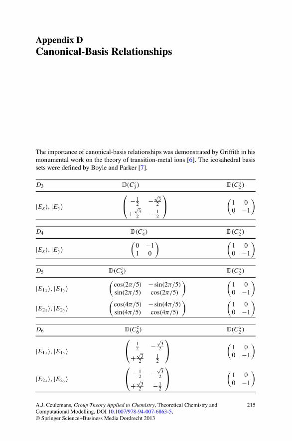
The importance of canonical-basis relationships was demonstrated by Griffith in hismonumental work on the theory of transition-metal ions [6]. The icosahedral basissets were defined by Boyle and Parker [7].
D3 D(Cz3) D(Cx
2 )
|Ex〉, |Ey〉⎛⎝ − 1
2 −√
32
+√
32 − 1
2
⎞⎠ (
1 00 −1
)
D4 D(Cz4) D(Cx
2 )
|Ex〉, |Ey〉(
0 −11 0
) (1 00 −1
)
D5 D(Cz5) D(Cx
2 )
|E1x〉, |E1y〉(
cos(2π/5) − sin(2π/5)
sin(2π/5) cos(2π/5)
) (1 00 −1
)
|E2x〉, |E2y〉(
cos(4π/5) − sin(4π/5)
sin(4π/5) cos(4π/5)
) (1 00 −1
)
D6 D(Cz6) D(Cx
2 )
|E1x〉, |E1y〉⎛⎝ 1
2 −√
32
+√
32
12
⎞⎠ (
1 00 −1
)
|E2x〉, |E2y〉⎛⎝ − 1
2 −√
32
+√
32 − 1
2
⎞⎠
(1 00 −1
)
A.J. Ceulemans, Group Theory Applied to Chemistry, Theoretical Chemistry andComputational Modelling, DOI 10.1007/978-94-007-6863-5,© Springer Science+Business Media Dordrecht 2013
215
216 D Canonical-Basis Relationships
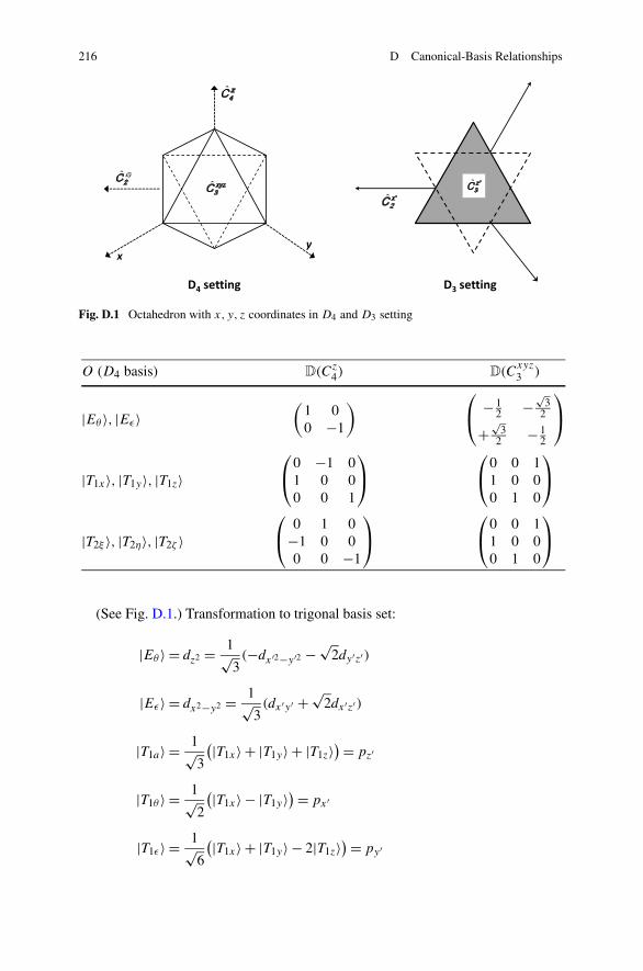
Fig. D.1 Octahedron with x, y, z coordinates in D4 and D3 setting
O (D4 basis) D(Cz4) D(C
xyz
3 )
|Eθ 〉, |Eε〉(
1 00 −1
) ⎛⎝ − 1
2 −√
32
+√
32 − 1
2
⎞⎠
|T1x〉, |T1y〉, |T1z〉⎛⎝0 −1 0
1 0 00 0 1
⎞⎠
⎛⎝0 0 1
1 0 00 1 0
⎞⎠
|T2ξ 〉, |T2η〉, |T2ζ 〉⎛⎝ 0 1 0
−1 0 00 0 −1
⎞⎠
⎛⎝0 0 1
1 0 00 1 0
⎞⎠
(See Fig. D.1.) Transformation to trigonal basis set:
|Eθ 〉 = dz2 = 1√3(−dx′2−y′2 − √
2dy′z′)
|Eε〉 = dx2−y2 = 1√3(dx′y′ + √
2dx′z′)
|T1a〉 = 1√3
(|T1x〉 + |T1y〉 + |T1z〉) = pz′
|T1θ 〉 = 1√2
(|T1x〉 − |T1y〉) = px′
|T1ε〉 = 1√6
(|T1x〉 + |T1y〉 − 2|T1z〉) = py′
D Canonical-Basis Relationships 217
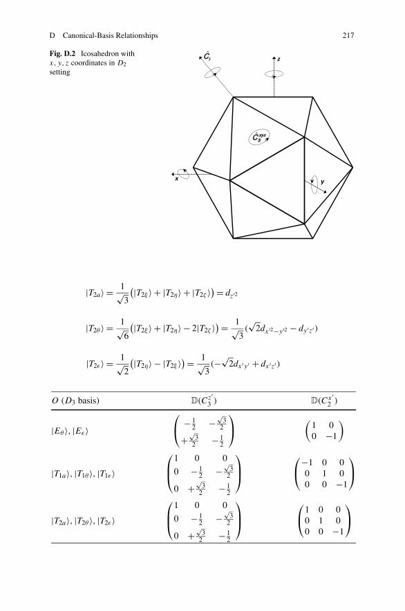
Fig. D.2 Icosahedron withx, y, z coordinates in D2setting
|T2a〉 = 1√3
(|T2ξ 〉 + |T2η〉 + |T2ζ 〉) = dz′2
|T2θ 〉 = 1√6
(|T2ξ 〉 + |T2η〉 − 2|T2ζ 〉) = 1√
3(√
2dx′2−y′2 − dy′z′)
|T2ε〉 = 1√2
(|T2η〉 − |T2ξ 〉) = 1√
3(−√
2dx′y′ + dx′z′)
O (D3 basis) D(Cz′3 ) D(Cx′
2 )
|Eθ 〉, |Eε〉⎛⎝ − 1
2 −√
32
+√
32 − 1
2
⎞⎠ (
1 00 −1
)
|T1a〉, |T1θ 〉, |T1ε〉⎛⎜⎝
1 0 0
0 − 12 −
√3
2
0 +√
32 − 1
2
⎞⎟⎠
⎛⎝−1 0 0
0 1 00 0 −1
⎞⎠
|T2a〉, |T2θ 〉, |T2ε〉⎛⎜⎝
1 0 0
0 − 12 −
√3
2
0 +√
32 − 1
2
⎞⎟⎠
⎛⎝1 0 0
0 1 00 0 −1
⎞⎠
218 D Canonical-Basis Relationships
I (D2 basis, Fig. D.2) D(C5) D(Cxyz
3 ) D(Cz2)
|T1x〉, |T1y〉, |T1z〉 12
⎛⎝ 1 −φ φ−1
φ φ−1 −1φ−1 1 φ
⎞⎠
⎛⎝0 0 1
1 0 00 1 0
⎞⎠
⎛⎝−1 0 0
0 −1 00 0 1
⎞⎠
|T2x〉, |T2y〉, |T2z〉 12
⎛⎝ 1 φ−1 −φ
−φ−1 −φ −1−φ 1 −φ−1
⎞⎠
⎛⎝0 0 1
1 0 00 1 0
⎞⎠
⎛⎝−1 0 0
0 −1 00 0 1
⎞⎠
|Ga〉, |Gx〉, |Gy〉,|Gz〉
14
⎛⎜⎜⎝
−1 −√5
√5
√5√
5 −3 −1 −1√5 1 −1 3
−√5 −1 −3 1
⎞⎟⎟⎠
⎛⎜⎜⎝
1 0 0 00 0 0 10 1 0 00 0 0 1
⎞⎟⎟⎠
⎛⎜⎜⎝
1 0 0 00 −1 0 00 0 −1 00 0 0 1
⎞⎟⎟⎠
I |Hθ〉, |Hε〉, |Hξ 〉, |Hη〉, |Hζ 〉
D(C5) D(Cxyz
3 ) D(Cz2)⎛
⎜⎜⎜⎜⎜⎜⎜⎜⎝
− 14 −
√3
41√8
1√2
− 1√8
−√
34
14 −
√3√8
0 −√
3√8
− 1√8
√3√8
0 12
12
1√2
0 − 12
12 0
1√8
√3√8
12 0 − 1
2
⎞⎟⎟⎟⎟⎟⎟⎟⎟⎠
⎛⎜⎜⎜⎜⎜⎜⎝
− 12 −
√3
2 0 0 0√3
2 − 12 0 0 0
0 0 0 0 1
0 0 1 0 0
0 0 0 1 0
⎞⎟⎟⎟⎟⎟⎟⎠
⎛⎜⎜⎜⎜⎜⎝
1 0 0 0 0
0 1 0 0 0
0 0 −1 0 0
0 0 0 −1 0
0 0 0 0 1
⎞⎟⎟⎟⎟⎟⎠
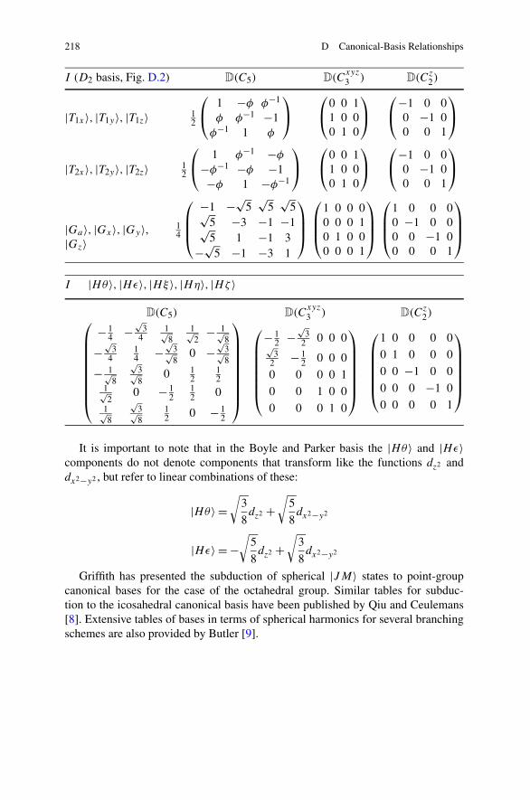
It is important to note that in the Boyle and Parker basis the |Hθ〉 and |Hε〉components do not denote components that transform like the functions dz2 anddx2−y2 , but refer to linear combinations of these:
|Hθ〉 =√
3
8dz2 +
√5
8dx2−y2
|Hε〉 = −√
5
8dz2 +
√3
8dx2−y2
Griffith has presented the subduction of spherical |JM〉 states to point-groupcanonical bases for the case of the octahedral group. Similar tables for subduc-tion to the icosahedral canonical basis have been published by Qiu and Ceulemans[8]. Extensive tables of bases in terms of spherical harmonics for several branchingschemes are also provided by Butler [9].
Appendix EDirect-Product Tables
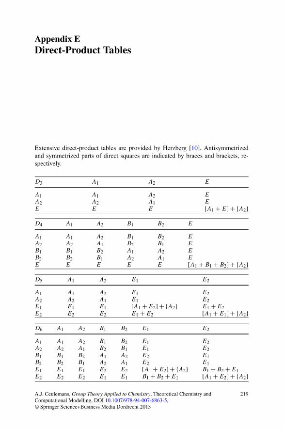
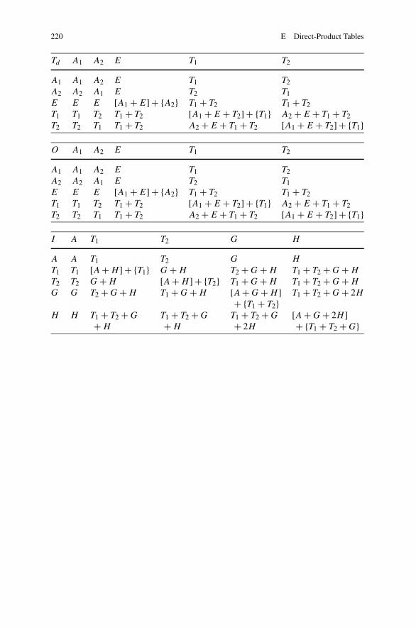
Extensive direct-product tables are provided by Herzberg [10]. Antisymmetrizedand symmetrized parts of direct squares are indicated by braces and brackets, re-spectively.
D3 A1 A2 E
A1 A1 A2 EA2 A2 A1 EE E E [A1 + E] + {A2}D4 A1 A2 B1 B2 E
A1 A1 A2 B1 B2 EA2 A2 A1 B2 B1 EB1 B1 B2 A1 A2 EB2 B2 B1 A2 A1 EE E E E E [A1 + B1 + B2] + {A2}D5 A1 A2 E1 E2
A1 A1 A2 E1 E2A2 A2 A1 E1 E2E1 E1 E1 [A1 + E2] + {A2} E1 + E2E2 E2 E2 E1 + E2 [A1 + E1] + {A2}D6 A1 A2 B1 B2 E1 E2
A1 A1 A2 B1 B2 E1 E2A2 A2 A1 B2 B1 E1 E2B1 B1 B2 A1 A2 E2 E1B2 B2 B1 A2 A1 E2 E1E1 E1 E1 E2 E2 [A1 + E2] + {A2} B1 + B2 + E1E2 E2 E2 E1 E1 B1 + B2 + E1 [A1 + E2] + {A2}
A.J. Ceulemans, Group Theory Applied to Chemistry, Theoretical Chemistry andComputational Modelling, DOI 10.1007/978-94-007-6863-5,© Springer Science+Business Media Dordrecht 2013
219
220 E Direct-Product Tables
Td A1 A2 E T1 T2
A1 A1 A2 E T1 T2A2 A2 A1 E T2 T1E E E [A1 + E] + {A2} T1 + T2 T1 + T2T1 T1 T2 T1 + T2 [A1 + E + T2] + {T1} A2 + E + T1 + T2T2 T2 T1 T1 + T2 A2 + E + T1 + T2 [A1 + E + T2] + {T1}
O A1 A2 E T1 T2
A1 A1 A2 E T1 T2A2 A2 A1 E T2 T1E E E [A1 + E] + {A2} T1 + T2 T1 + T2T1 T1 T2 T1 + T2 [A1 + E + T2] + {T1} A2 + E + T1 + T2T2 T2 T1 T1 + T2 A2 + E + T1 + T2 [A1 + E + T2] + {T1}
I A T1 T2 G H
A A T1 T2 G H
T1 T1 [A + H ] + {T1} G + H T2 + G + H T1 + T2 + G + H
T2 T2 G + H [A + H ] + {T2} T1 + G + H T1 + T2 + G + H
G G T2 + G + H T1 + G + H [A + G + H ] T1 + T2 + G + 2H
+ {T1 + T2}H H T1 + T2 + G T1 + T2 + G T1 + T2 + G [A + G + 2H ]
+ H + H + 2H + {T1 + T2 + G}
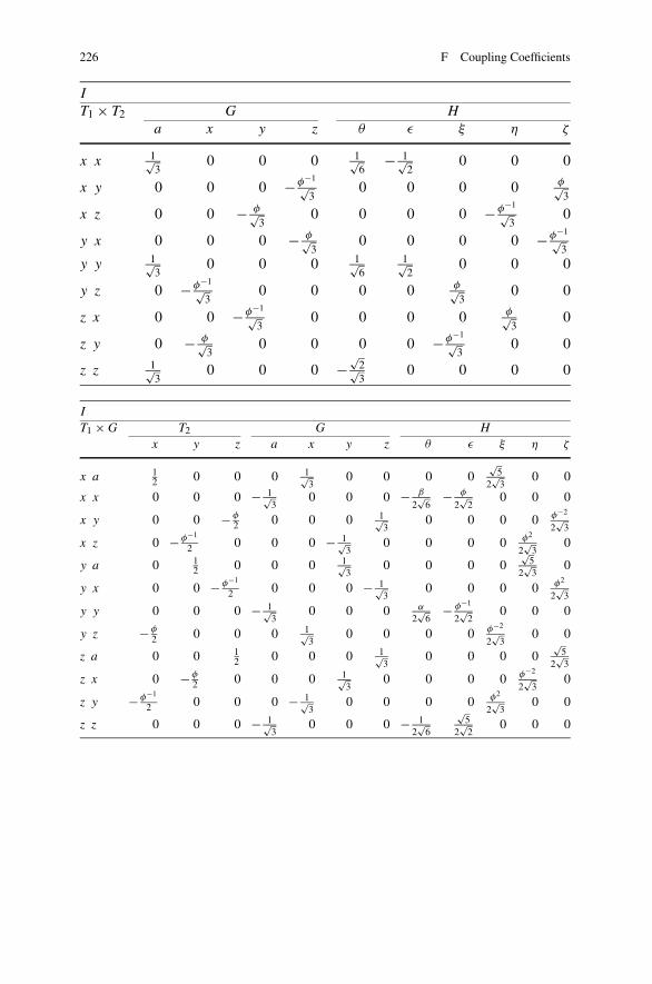
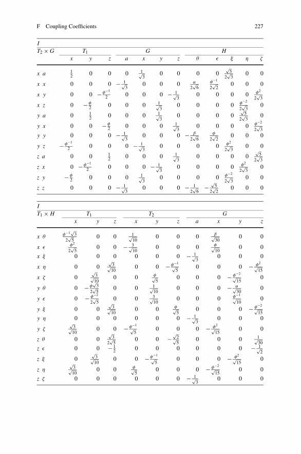
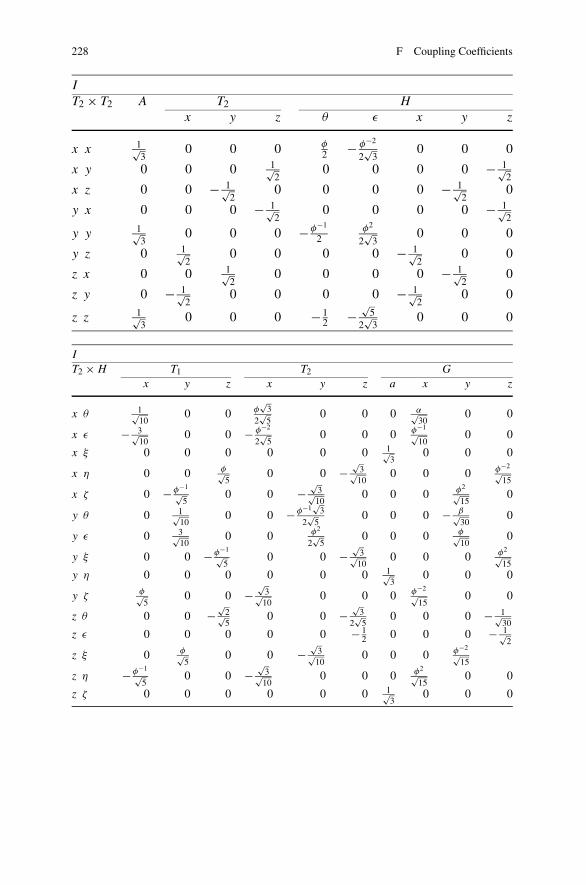
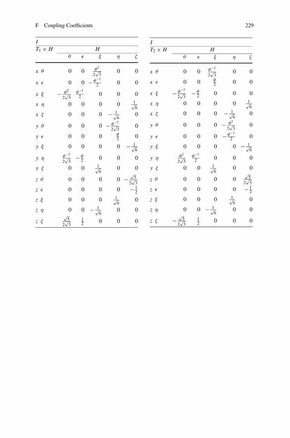
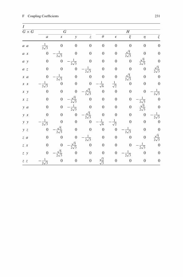
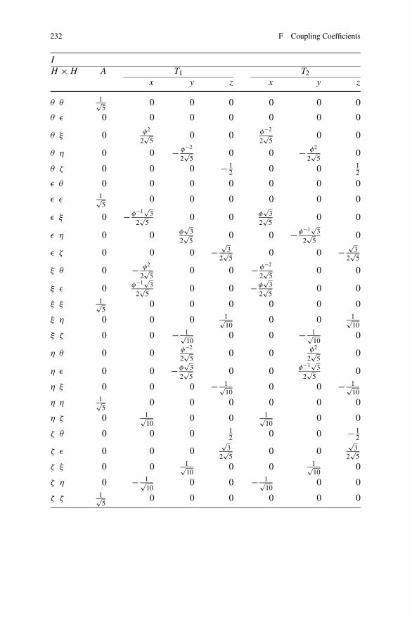
Appendix FCoupling Coefficients
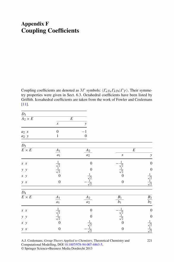
Coupling coefficients are denoted as 3Γ symbols: 〈ΓaγaΓbγb|Γ γ 〉. Their symme-try properties were given in Sect. 6.3. Octahedral coefficients have been listed byGriffith. Icosahedral coefficients are taken from the work of Fowler and Ceulemans[11].
D3A2 × E E
x y
a2 x 0 −1a2 y 1 0
D3E × E A1 A2 E
a1 a2 x y
x x 1√2
0 − 1√2
0
y y 1√2
0 1√2
0
x y 0 1√2
0 1√2
y x 0 − 1√2
0 1√2
D4E × E A1 A2 B1 B2
a1 a2 b1 b2
x x 1√2
0 − 1√2
0
y y 1√2
0 1√2
0
x y 0 1√2
0 1√2
y x 0 − 1√2
0 1√2
A.J. Ceulemans, Group Theory Applied to Chemistry, Theoretical Chemistry andComputational Modelling, DOI 10.1007/978-94-007-6863-5,© Springer Science+Business Media Dordrecht 2013
221
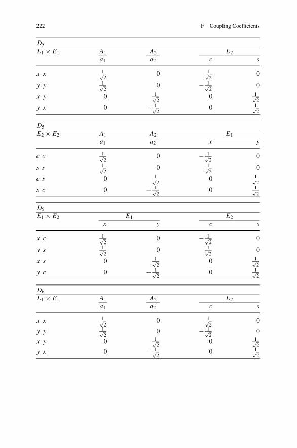
222 F Coupling Coefficients
D5E1 × E1 A1 A2 E2
a1 a2 c s
x x 1√2
0 1√2
0
y y 1√2
0 − 1√2
0
x y 0 1√2
0 1√2
y x 0 − 1√2
0 1√2
D5E2 × E2 A1 A2 E1
a1 a2 x y
c c 1√2
0 − 1√2
0
s s 1√2
0 1√2
0
c s 0 1√2
0 1√2
s c 0 − 1√2
0 1√2
D5E1 × E2 E1 E2
x y c s
x c 1√2
0 − 1√2
0
y s 1√2
0 1√2
0
x s 0 1√2
0 1√2
y c 0 − 1√2
0 1√2
D6E1 × E1 A1 A2 E2
a1 a2 c s
x x 1√2
0 1√2
0
y y 1√2
0 − 1√2
0
x y 0 1√2
0 1√2
y x 0 − 1√2
0 1√2
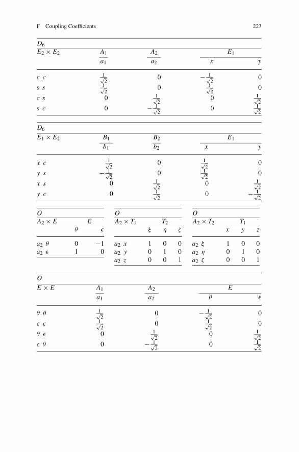
F Coupling Coefficients 223
D6E2 × E2 A1 A2 E1
a1 a2 x y
c c 1√2
0 − 1√2
0
s s 1√2
0 1√2
0
c s 0 1√2
0 1√2
s c 0 − 1√2
0 1√2
D6
E1 × E2 B1 B2 E1
b1 b2 x y
x c 1√2
0 1√2
0
y s − 1√2
0 1√2
0
x s 0 1√2
0 1√2
y c 0 1√2
0 − 1√2
O
A2 × E E
θ ε
a2 θ 0 −1a2 ε 1 0
O
A2 × T1 T2ξ η ζ
a2 x 1 0 0a2 y 0 1 0a2 z 0 0 1
O
A2 × T2 T1x y z
a2 ξ 1 0 0a2 η 0 1 0a2 ζ 0 0 1
O
E × E A1 A2 E
a1 a2 θ ε
θ θ 1√2
0 − 1√2
0
ε ε 1√2
0 1√2
0
θ ε 0 1√2
0 1√2
ε θ 0 − 1√2
0 1√2
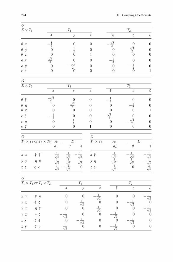
224 F Coupling Coefficients
O
E × T1 T1 T2x y z ξ η ζ
θ x − 12 0 0 −
√3
2 0 0
θ y 0 − 12 0 0
√3
2 0θ z 0 0 1 0 0 0
ε x√
32 0 0 − 1
2 0 0
ε y 0 −√
32 0 0 − 1
2 0ε z 0 0 0 0 0 1
O
E × T2 T1 T2x y z ξ η ζ
θ ξ −√3
2 0 0 − 12 0 0
θ η 0√
32 0 0 − 1
2 0θ ζ 0 0 0 0 0 1
ε ξ − 12 0 0
√3
2 0 0
ε η 0 − 12 0 0 −
√3
2 0ε ζ 0 0 1 0 0 0
O
T1 × T1 or T2 × T2 A1 E
a1 θ ε
x x ξ ξ 1√3
1√6
− 1√2
y y η η 1√3
1√6
1√2
z z ζ ζ 1√3
− 2√6
0
O
T1 × T2 A2 E
a2 θ ε
x ξ 1√3
− 1√2
− 1√6
y η 1√3
1√2
− 1√6
z ζ 1√3
0 2√6
O
T1 × T1 or T2 × T2 T1 T2x y z ξ η ζ
x y ξ η 0 0 − 1√2
0 0 − 1√2
x z ξ ζ 0 1√2
0 0 − 1√2
0
y x η ξ 0 0 1√2
0 0 − 1√2
y z η ζ − 1√2
0 0 − 1√2
0 0
z x ζ ξ 0 − 1√2
0 0 − 1√2
0
z y ζ η 1√2
0 0 − 1√2
0 0
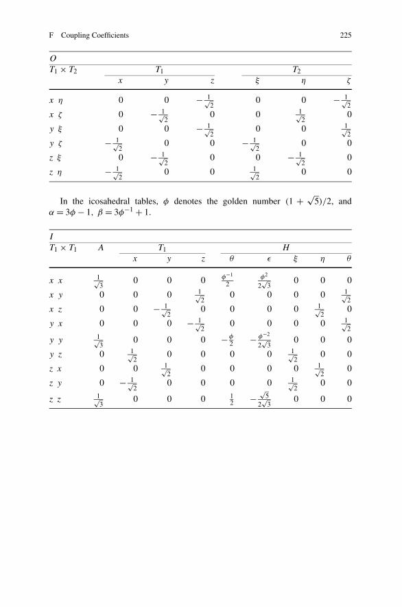
F Coupling Coefficients 225
O
T1 × T2 T1 T2x y z ξ η ζ
x η 0 0 − 1√2
0 0 − 1√2
x ζ 0 − 1√2
0 0 1√2
0
y ξ 0 0 − 1√2
0 0 1√2
y ζ − 1√2
0 0 − 1√2
0 0
z ξ 0 − 1√2
0 0 − 1√2
0
z η − 1√2
0 0 1√2
0 0
In the icosahedral tables, φ denotes the golden number (1 + √5)/2, and
α = 3φ − 1, β = 3φ−1 + 1.
I
T1 × T1 A T1 H
x y z θ ε ξ η θ
x x 1√3
0 0 0 φ−1
2φ2
2√
30 0 0
x y 0 0 0 1√2
0 0 0 0 1√2
x z 0 0 − 1√2
0 0 0 0 1√2
0
y x 0 0 0 − 1√2
0 0 0 0 1√2
y y 1√3
0 0 0 −φ2 − φ−2
2√
30 0 0
y z 0 1√2
0 0 0 0 1√2
0 0
z x 0 0 1√2
0 0 0 0 1√2
0
z y 0 − 1√2
0 0 0 0 1√2
0 0
z z 1√3
0 0 0 12 −
√5
2√
30 0 0
226 F Coupling Coefficients
I
T1 × T2 G H
a x y z θ ε ξ η ζ
x x 1√3
0 0 0 1√6
− 1√2
0 0 0
x y 0 0 0 −φ−1√3
0 0 0 0 φ√3
x z 0 0 − φ√3
0 0 0 0 −φ−1√3
0
y x 0 0 0 − φ√3
0 0 0 0 −φ−1√3
y y 1√3
0 0 0 1√6
1√2
0 0 0
y z 0 −φ−1√3
0 0 0 0 φ√3
0 0
z x 0 0 −φ−1√3
0 0 0 0 φ√3
0
z y 0 − φ√3
0 0 0 0 −φ−1√3
0 0
z z 1√3
0 0 0 −√
2√3
0 0 0 0
I
T1 × G T2 G H
x y z a x y z θ ε ξ η ζ
x a 12 0 0 0 1√
30 0 0 0
√5
2√
30 0
x x 0 0 0 − 1√3
0 0 0 − β
2√
6− φ
2√
20 0 0
x y 0 0 − φ2 0 0 0 1√
30 0 0 0 φ−2
2√
3
x z 0 − φ−1
2 0 0 0 − 1√3
0 0 0 0 φ2
2√
30
y a 0 12 0 0 0 1√
30 0 0 0
√5
2√
30
y x 0 0 − φ−1
2 0 0 0 − 1√3
0 0 0 0 φ2
2√
3
y y 0 0 0 − 1√3
0 0 0 α
2√
6− φ−1
2√
20 0 0
y z − φ2 0 0 0 1√
30 0 0 0 φ−2
2√
30 0
z a 0 0 12 0 0 0 1√
30 0 0 0
√5
2√
3
z x 0 − φ2 0 0 0 1√
30 0 0 0 φ−2
2√
30
z y − φ−1
2 0 0 0 − 1√3
0 0 0 0 φ2
2√
30 0
z z 0 0 0 − 1√3
0 0 0 − 12√
6
√5
2√
20 0 0
F Coupling Coefficients 227
I
T2 × G T1 G H
x y z a x y z θ ε ξ η ζ
x a 12 0 0 0 1√
30 0 0 0
√5
2√
30 0
x x 0 0 0 − 1√3
0 0 0 α
2√
6φ−1
2√
20 0 0
x y 0 0 − φ−1
2 0 0 0 − 1√3
0 0 0 0 φ2
2√
3
x z 0 − φ2 0 0 0 1√
30 0 0 0 φ−2
2√
30
y a 0 12 0 0 0 1√
30 0 0 0
√5
2√
30
y x 0 0 − φ2 0 0 0 1√
30 0 0 0 φ−2
2√
3y y 0 0 0 − 1√
30 0 0 − β
2√
6φ
2√
20 0 0
y z − φ−1
2 0 0 0 − 1√3
0 0 0 0 φ2
2√
30 0
z a 0 0 12 0 0 0 1√
30 0 0 0
√5
2√
3
z x 0 − φ−1
2 0 0 0 − 1√3
0 0 0 0 φ2
2√
30
z y − φ2 0 0 0 1√
30 0 0 0 φ−2
2√
30 0
z z 0 0 0 − 1√3
0 0 0 − 12√
6−
√5
2√
20 0 0
I
T1 × H T1 T2 G
x y z x y z a x y z
x θφ−1
√3
2√
50 0 1√
100 0 0 β√
300 0
x εφ2
2√
50 0 − 3√
100 0 0 φ√
100 0
x ξ 0 0 0 0 0 0 − 1√3
0 0 0
x η 0 0√
3√10
0 0 − φ−1√5
0 0 0 − φ2√15
x ζ 0√
3√10
0 0 φ√5
0 0 0 − φ−2√15
0
y θ 0 − φ√
32√
50 0 1√
100 0 0 − α√
300
y ε 0 − φ−2
2√
50 0 3√
100 0 0 φ−1√
100
y ξ 0 0√
3√10
0 0 φ√5
0 0 0 − φ−2√15
y η 0 0 0 0 0 0 − 1√3
0 0 0
y ζ√
3√10
0 0 − φ−1√5
0 0 0 − φ2√15
0 0
z θ 0 0√
32√
50 0 −
√2√5
0 0 0 1√30
z ε 0 0 − 12 0 0 0 0 0 0 − 1√
2
z ξ 0√
3√10
0 0 − φ−1√5
0 0 0 − φ2√15
0
z η√
3√10
0 0 φ√5
0 0 0 − φ−2√15
0 0
z ζ 0 0 0 0 0 0 − 1√3
0 0 0
228 F Coupling Coefficients
I
T2 × T2 A T2 H
x y z θ ε x y z
x x 1√3
0 0 0 φ2 − φ−2
2√
30 0 0
x y 0 0 0 1√2
0 0 0 0 − 1√2
x z 0 0 − 1√2
0 0 0 0 − 1√2
0
y x 0 0 0 − 1√2
0 0 0 0 − 1√2
y y 1√3
0 0 0 −φ−1
2φ2
2√
30 0 0
y z 0 1√2
0 0 0 0 − 1√2
0 0
z x 0 0 1√2
0 0 0 0 − 1√2
0
z y 0 − 1√2
0 0 0 0 − 1√2
0 0
z z 1√3
0 0 0 − 12 −
√5
2√
30 0 0
I
T2 × H T1 T2 G
x y z x y z a x y z
x θ 1√10
0 0 φ√
32√
50 0 0 α√
300 0
x ε − 3√10
0 0 − φ−2
2√
50 0 0 φ−1√
100 0
x ξ 0 0 0 0 0 0 1√3
0 0 0
x η 0 0 φ√5
0 0 −√
3√10
0 0 0 φ−2√15
x ζ 0 − φ−1√5
0 0 −√
3√10
0 0 0 φ2√15
0
y θ 0 1√10
0 0 − φ−1√
32√
50 0 0 − β√
300
y ε 0 3√10
0 0 φ2
2√
50 0 0 φ√
100
y ξ 0 0 − φ−1√5
0 0 −√
3√10
0 0 0 φ2√15
y η 0 0 0 0 0 0 1√3
0 0 0
y ζφ√5
0 0 −√
3√10
0 0 0 φ−2√15
0 0
z θ 0 0 −√
2√5
0 0 −√
32√
50 0 0 − 1√
30z ε 0 0 0 0 0 − 1
2 0 0 0 − 1√2
z ξ 0 φ√5
0 0 −√
3√10
0 0 0 φ−2√15
z η − φ−1√5
0 0 −√
3√10
0 0 0 φ2√15
0 0
z ζ 0 0 0 0 0 0 1√3
0 0 0
F Coupling Coefficients 229
I
T1 × H H
θ ε ξ η ζ
x θ 0 0 φ2
2√
30 0
x ε 0 0 − φ−1
2 0 0
x ξ − φ2
2√
3φ−1
2 0 0 0
x η 0 0 0 0 1√6
x ζ 0 0 0 − 1√6
0
y θ 0 0 0 − φ−2
2√
30
y ε 0 0 0 φ2 0
y ξ 0 0 0 0 − 1√6
y ηφ−2
2√
3− φ
2 0 0 0
y ζ 0 0 1√6
0 0
z θ 0 0 0 0 −√
52√
3
z ε 0 0 0 0 − 12
z ξ 0 0 0 1√6
0
z η 0 0 − 1√6
0 0
z ζ√
52√
312 0 0 0
I
T2 × H H
θ ε ξ η ζ
x θ 0 0 φ−2
2√
30 0
x ε 0 0 φ2 0 0
x ξ − φ−2
2√
3− φ
2 0 0 0
x η 0 0 0 0 1√6
x ζ 0 0 0 − 1√6
0
y θ 0 0 0 − φ2
2√
30
y ε 0 0 0 − φ−1
2 0
y ξ 0 0 0 0 − 1√6
y ηφ2
2√
3φ−1
2 0 0 0
y ζ 0 0 1√6
0 0
z θ 0 0 0 0√
52√
3
z ε 0 0 0 0 − 12
z ξ 0 0 0 1√6
0
z η 0 0 − 1√6
0 0
z ζ −√
52√
312 0 0 0
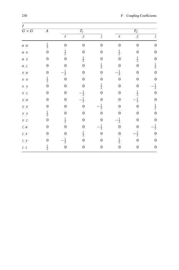
230 F Coupling Coefficients
I
G × G A T1 T2
x y z x y z
a a 12 0 0 0 0 0 0
a x 0 12 0 0 1
2 0 0
a y 0 0 12 0 0 1
2 0
a z 0 0 0 12 0 0 1
2
x a 0 − 12 0 0 − 1
2 0 0
x x 12 0 0 0 0 0 0
x y 0 0 0 12 0 0 − 1
2
x z 0 0 − 12 0 0 1
2 0
y a 0 0 − 12 0 0 − 1
2 0
y x 0 0 0 − 12 0 0 1
2
y y 12 0 0 0 0 0 0
y z 0 12 0 0 − 1
2 0 0
z a 0 0 0 − 12 0 0 − 1
2
z x 0 0 12 0 0 − 1
2 0
z y 0 − 12 0 0 1
2 0 0
z z 12 0 0 0 0 0 0
F Coupling Coefficients 231
I
G × G G H
a x y z θ ε ξ η ζ
a a 12√
30 0 0 0 0 0 0 0
a x 0 − 12√
30 0 0 0
√5
2√
30 0
a y 0 0 − 12√
30 0 0 0
√5
2√
30
a z 0 0 0 − 12√
30 0 0 0
√5
2√
3
x a 0 − 12√
30 0 0 0
√5
2√
30 0
x x − 12√
30 0 0 − 1√
61√2
0 0 0
x y 0 0 0 −√
52√
30 0 0 0 − 1
2√
3
x z 0 0 −√
52√
30 0 0 0 − 1
2√
30
y a 0 0 − 12√
30 0 0 0
√5
2√
30
y x 0 0 0 −√
52√
30 0 0 0 − 1
2√
3
y y − 12√
30 0 0 − 1√
6− 1√
20 0 0
y z 0 −√
52√
30 0 0 0 − 1
2√
30 0
z a 0 0 0 − 12√
30 0 0 0
√5
2√
3
z x 0 0 −√
52√
30 0 0 0 − 1
2√
30
z y 0 −√
52√
30 0 0 0 − 1
2√
30 0
z z − 12√
30 0 0
√2√3
0 0 0 0
232 F Coupling Coefficients
I
H × H A T1 T2x y z x y z
θ θ 1√5
0 0 0 0 0 0
θ ε 0 0 0 0 0 0 0
θ ξ 0 φ2
2√
50 0 φ−2
2√
50 0
θ η 0 0 − φ−2
2√
50 0 − φ2
2√
50
θ ζ 0 0 0 − 12 0 0 1
2
ε θ 0 0 0 0 0 0 0
ε ε 1√5
0 0 0 0 0 0
ε ξ 0 −φ−1√
32√
50 0 φ
√3
2√
50 0
ε η 0 0 φ√
32√
50 0 −φ−1
√3
2√
50
ε ζ 0 0 0 −√
32√
50 0 −
√3
2√
5
ξ θ 0 − φ2
2√
50 0 − φ−2
2√
50 0
ξ ε 0 φ−1√
32√
50 0 −φ
√3
2√
50 0
ξ ξ 1√5
0 0 0 0 0 0
ξ η 0 0 0 1√10
0 0 1√10
ξ ζ 0 0 − 1√10
0 0 − 1√10
0
η θ 0 0 φ−2
2√
50 0 φ2
2√
50
η ε 0 0 −φ√
32√
50 0 φ−1
√3
2√
50
η ξ 0 0 0 − 1√10
0 0 − 1√10
η η 1√5
0 0 0 0 0 0
η ζ 0 1√10
0 0 1√10
0 0
ζ θ 0 0 0 12 0 0 − 1
2
ζ ε 0 0 0√
32√
50 0
√3
2√
5
ζ ξ 0 0 1√10
0 0 1√10
0
ζ η 0 − 1√10
0 0 − 1√10
0 0
ζ ζ 1√5
0 0 0 0 0 0
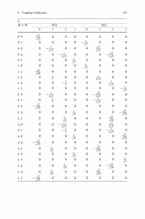
F Coupling Coefficients 233
I
H × H [G] {G}a x y z a x y z
θ θ√
3√10
0 0 0 0 0 0 0
θ ε 0 0 0 0 − 1√2
0 0 0
θ ξ 0 − 12√
30 0 0
√3
2√
50 0
θ η 0 0 − 12√
30 0 0 −
√3
2√
50
θ ζ 0 0 0 1√3
0 0 0 0
ε θ 0 0 0 0 1√2
0 0 0
ε ε√
3√10
0 0 0 0 0 0 0
ε ξ 0 12 0 0 0 1
2√
50 0
ε η 0 0 − 12 0 0 0 1
2√
50
ε ζ 0 0 0 0 0 0 0 − 1√5
ξ θ 0 − 12√
30 0 0 −
√3
2√
50 0
ξ ε 0 12 0 0 0 − 1
2√
50 0
ξ ξ −√
2√15
0 0 0 0 0 0 0
ξ η 0 0 0 1√6
0 0 0 −√
3√10
ξ ζ 0 0 1√6
0 0 0√
3√10
0
η θ 0 0 − 12√
30 0 0
√3
2√
50
η ε 0 0 − 12 0 0 0 − 1
2√
50
η ξ 0 0 0 1√6
0 0 0√
3√10
η η −√
2√15
0 0 0 0 0 0 0
η ζ 0 1√6
0 0 0 −√
3√10
0 0
ζ θ 0 0 0 1√3
0 0 0 0
ζ ε 0 0 0 0 0 0 0 1√5
ζ ξ 0 0 1√6
0 0 0 −√
3√10
0
ζ η 0 1√6
0 0 0√
3√10
0 0
ζ ζ −√
2√15
0 0 0 0 0 0 0
234 F Coupling Coefficients
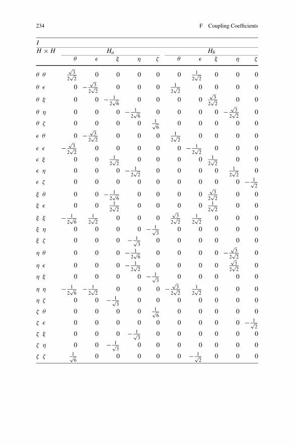
I
H × H Ha Hb
θ ε ξ η ζ θ ε ξ η ζ
θ θ√
32√
20 0 0 0 0 1
2√
20 0 0
θ ε 0 −√
32√
20 0 0 1
2√
20 0 0 0
θ ξ 0 0 − 12√
60 0 0 0
√3
2√
20 0
θ η 0 0 0 − 12√
60 0 0 0 −
√3
2√
20
θ ζ 0 0 0 0 1√6
0 0 0 0 0
ε θ 0 −√
32√
20 0 0 1
2√
20 0 0 0
ε ε −√
32√
20 0 0 0 0 − 1
2√
20 0 0
ε ξ 0 0 12√
20 0 0 0 1
2√
20 0
ε η 0 0 0 − 12√
20 0 0 0 1
2√
20
ε ζ 0 0 0 0 0 0 0 0 0 − 1√2
ξ θ 0 0 − 12√
60 0 0 0
√3
2√
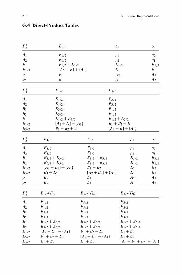
20 0
ξ ε 0 0 12√
20 0 0 0 1
2√
20 0
ξ ξ − 12√
61
2√
20 0 0
√3
2√
21
2√
20 0 0
ξ η 0 0 0 0 − 1√3
0 0 0 0 0
ξ ζ 0 0 0 − 1√3
0 0 0 0 0 0
η θ 0 0 0 − 12√
60 0 0 0 −
√3
2√
20
η ε 0 0 0 − 12√
20 0 0 0
√1
2√
20
η ξ 0 0 0 0 − 1√3
0 0 0 0 0
η η − 12√
6− 1
2√
20 0 0 −
√3
2√
21
2√
20 0 0
η ζ 0 0 − 1√3
0 0 0 0 0 0 0
ζ θ 0 0 0 0 1√6
0 0 0 0 0
ζ ε 0 0 0 0 0 0 0 0 0 − 1√2
ζ ξ 0 0 0 − 1√3
0 0 0 0 0 0
ζ η 0 0 − 1√3
0 0 0 0 0 0 0
ζ ζ 1√6
0 0 0 0 0 − 1√2
0 0 0
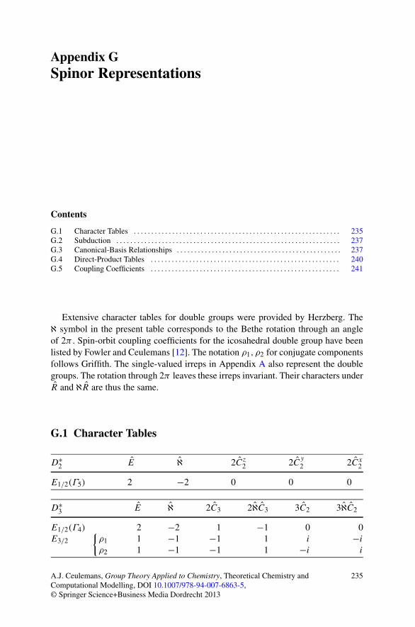
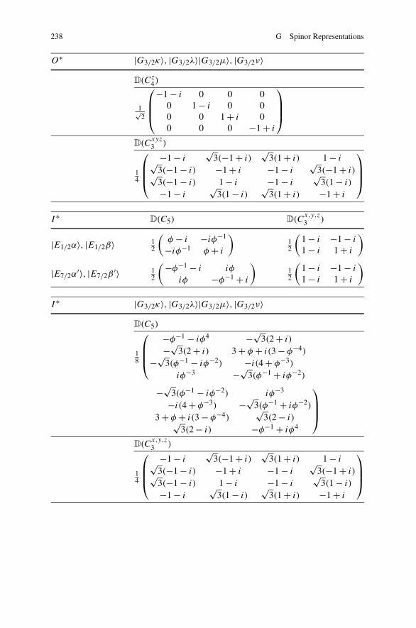
Appendix GSpinor Representations
Contents
G.1 Character Tables . . . . . . . . . . . . . . . . . . . . . . . . . . . . . . . . . . . . . . . . . . . . . . . . . . . . . . . . . . . 235G.2 Subduction . . . . . . . . . . . . . . . . . . . . . . . . . . . . . . . . . . . . . . . . . . . . . . . . . . . . . . . . . . . . . . . . 237G.3 Canonical-Basis Relationships . . . . . . . . . . . . . . . . . . . . . . . . . . . . . . . . . . . . . . . . . . . . . . . 237G.4 Direct-Product Tables . . . . . . . . . . . . . . . . . . . . . . . . . . . . . . . . . . . . . . . . . . . . . . . . . . . . . . 240G.5 Coupling Coefficients . . . . . . . . . . . . . . . . . . . . . . . . . . . . . . . . . . . . . . . . . . . . . . . . . . . . . . 241
Extensive character tables for double groups were provided by Herzberg. Theℵ symbol in the present table corresponds to the Bethe rotation through an angleof 2π . Spin-orbit coupling coefficients for the icosahedral double group have beenlisted by Fowler and Ceulemans [12]. The notation ρ1, ρ2 for conjugate componentsfollows Griffith. The single-valued irreps in Appendix A also represent the doublegroups. The rotation through 2π leaves these irreps invariant. Their characters underR and ℵR are thus the same.
G.1 Character Tables
D∗2 E ℵ 2Cz
2 2Cy
2 2Cx2
E1/2(Γ5) 2 −2 0 0 0
D∗3 E ℵ 2C3 2ℵC3 3C2 3ℵC2
E1/2(Γ4) 2 −2 1 −1 0 0E3/2
{ρ1 1 −1 −1 1 i −i
ρ2 1 −1 −1 1 −i i
A.J. Ceulemans, Group Theory Applied to Chemistry, Theoretical Chemistry andComputational Modelling, DOI 10.1007/978-94-007-6863-5,© Springer Science+Business Media Dordrecht 2013
235
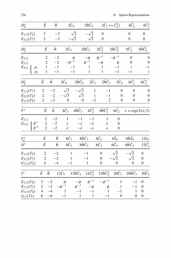
236 G Spinor Representations
D∗4 E ℵ 2C4 2ℵC4 2C2 (= C2
4) 4C′2 4C′′
2
E1/2(Γ6) 2 −2√
2 −√2 0 0 0
E3/2(Γ7) 2 −2 −√2
√2 0 0 0
D∗5 E ℵ 2C5 2ℵC5 2C2
5 2ℵC25 5C′
2 5ℵC′2
E1/2 2 −2 φ −φ φ−1 −φ−1 0 0E3/2 2 −2 −φ−1 φ−1 −φ φ 0 0E5/2
{ρ1 1 −1 −1 1 1 −1 i −i
ρ2 1 −1 −1 1 1 −1 −i i
D∗6 E ℵ 2C6 2ℵC6 2C3 2ℵC3 2C2 6C′
2 6C′′2
E1/2(Γ7) 2 −2√
3 −√3 1 −1 0 0 0
E5/2(Γ8) 2 −2 −√3
√3 1 −1 0 0 0
E3/2(Γ9) 2 −2 0 0 −2 2 0 0 0
T ∗ E ℵ 4C3 4ℵC3 4C23 4ℵC2
3 6C2 ε = exp(2πi/3)
E1/2 2 −2 1 −1 −1 1 0G3/2
{E′′ 2 −2 ε −ε −ε ε 0E′′′ 2 −2 ε −ε −ε ε 0
T ∗d E ℵ 8C3 8ℵC3 6C2 6S4 6ℵS4 12σd
O∗ E ℵ 8C3 8ℵC3 6C2 6C4 6ℵC4 12C′2
E1/2(Γ6) 2 −2 1 −1 0√
2 −√2 0
E5/2(Γ7) 2 −2 1 −1 0 −√2
√2 0
G3/2(Γ8) 4 −4 −1 1 0 0 0 0
I ∗ E ℵ 12C5 12ℵC5 12C25 12ℵC2
5 20C3 20ℵC3 30C2
E1/2(Γ6) 2 −2 φ −φ φ−1 −φ−1 1 −1 0E7/2(Γ7) 2 −2 −φ−1 φ−1 −φ φ 1 −1 0G3/2(Γ8) 4 −4 1 −1 −1 1 −1 1 0I5/2(Γ9) 6 −6 −1 1 1 −1 0 0 0
G.2 Subduction 237
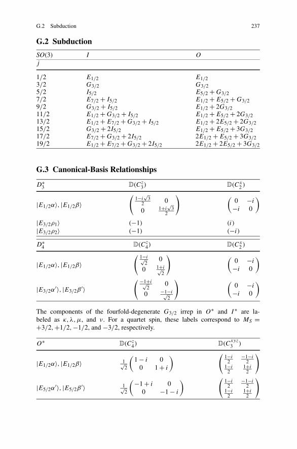
G.2 Subduction
SO(3) I O
j
1/2 E1/2 E1/23/2 G3/2 G3/25/2 I5/2 E5/2 + G3/27/2 E7/2 + I5/2 E1/2 + E5/2 + G3/29/2 G3/2 + I5/2 E1/2 + 2G3/211/2 E1/2 + G3/2 + I5/2 E1/2 + E5/2 + 2G3/213/2 E1/2 + E7/2 + G3/2 + I5/2 E1/2 + 2E5/2 + 2G3/215/2 G3/2 + 2I5/2 E1/2 + E5/2 + 3G3/217/2 E7/2 + G3/2 + 2I5/2 2E1/2 + E5/2 + 3G3/219/2 E1/2 + E7/2 + G3/2 + 2I5/2 2E1/2 + 2E5/2 + 3G3/2
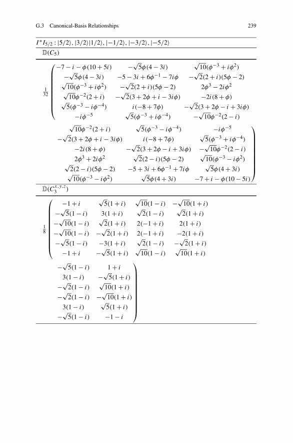
G.3 Canonical-Basis Relationships
D∗3 D(Cz
3) D(Cx2 )
|E1/2α〉, |E1/2β〉(
1−i√
32 0
0 1+i√
32
) (0 −i
−i 0
)
|E3/2ρ1〉 (−1) (i)
|E3/2ρ2〉 (−1) (−i)
D∗4 D(Cz
4) D(Cx2 )
|E1/2α〉, |E1/2β〉(
1−i√2
0
0 1+i√2
) (0 −i
−i 0
)
|E3/2α′〉, |E3/2β
′〉( −1+i√
20
0 −1−i√2
) (0 −i
−i 0
)
The components of the fourfold-degenerate G3/2 irrep in O∗ and I ∗ are la-beled as κ,λ,μ, and ν. For a quartet spin, these labels correspond to MS =+3/2,+1/2,−1/2, and −3/2, respectively.
O∗D(Cz
4) D(Cxyz
3 )
|E1/2α〉, |E1/2β〉 1√2
(1 − i 0
0 1 + i
) (1−i
2−1−i
21−i
21+i
2
)
|E5/2α′〉, |E5/2β
′〉 1√2
(−1 + i 00 −1 − i
) (1−i
2−1−i
21−i
21+i
2
)
238 G Spinor Representations
O∗ |G3/2κ〉, |G3/2λ〉|G3/2μ〉, |G3/2ν〉D(Cz
4)
1√2
⎛⎜⎜⎝
−1 − i 0 0 00 1 − i 0 00 0 1 + i 00 0 0 −1 + i
⎞⎟⎟⎠
D(Cxyz
3 )
14
⎛⎜⎜⎝
−1 − i√
3(−1 + i)√
3(1 + i) 1 − i√3(−1 − i) −1 + i −1 − i
√3(−1 + i)√
3(−1 − i) 1 − i −1 − i√
3(1 − i)
−1 − i√
3(1 − i)√
3(1 + i) −1 + i
⎞⎟⎟⎠
I ∗D(C5) D(C
x,y,z
3 )
|E1/2α〉, |E1/2β〉 12
(φ − i −iφ−1
−iφ−1 φ + i
)12
(1 − i −1 − i
1 − i 1 + i
)
|E7/2α′〉, |E7/2β
′〉 12
(−φ−1 − i iφ
iφ −φ−1 + i
)12
(1 − i −1 − i
1 − i 1 + i
)
I ∗ |G3/2κ〉, |G3/2λ〉|G3/2μ〉, |G3/2ν〉D(C5)
18
⎛⎜⎜⎝
−φ−1 − iφ4 −√3(2 + i)
−√3(2 + i) 3 + φ + i(3 − φ−4)
−√3(φ−1 − iφ−2) −i(4 + φ−3)
iφ−3 −√3(φ−1 + iφ−2)
−√3(φ−1 − iφ−2) iφ−3
−i(4 + φ−3) −√3(φ−1 + iφ−2)
3 + φ + i(3 − φ−4)√
3(2 − i)√3(2 − i) −φ−1 + iφ4
⎞⎟⎟⎠
D(Cx,y,z
3 )
14
⎛⎜⎜⎝
−1 − i√
3(−1 + i)√
3(1 + i) 1 − i√3(−1 − i) −1 + i −1 − i
√3(−1 + i)√
3(−1 − i) 1 − i −1 − i√
3(1 − i)
−1 − i√
3(1 − i)√
3(1 + i) −1 + i
⎞⎟⎟⎠
G.3 Canonical-Basis Relationships 239
I ∗I5/2 : |5/2〉, |3/2〉|1/2〉, |−1/2〉, |−3/2〉, |−5/2〉D(C5)
132
⎛⎜⎜⎜⎜⎜⎜⎜⎜⎝
−7 − i − φ(10 + 5i) −√5φ(4 − 3i)
√10(φ−3 + iφ2)
−√5φ(4 − 3i) −5 − 3i + 6φ−1 − 7iφ −√
2(2 + i)(5φ − 2)√10(φ−3 + iφ2) −√
2(2 + i)(5φ − 2) 2φ3 − 2iφ2√
10φ−2(2 + i) −√2(3 + 2φ + i − 3iφ) −2i(8 + φ)√
5(φ−3 − iφ−4) i(−8 + 7φ) −√2(3 + 2φ − i + 3iφ)
−iφ−5√
5(φ−3 + iφ−4) −√10φ−2(2 − i)
√10φ−2(2 + i)
√5(φ−3 − iφ−4) −iφ−5
−√2(3 + 2φ + i − 3iφ) i(−8 + 7φ)
√5(φ−3 + iφ−4)
−2i(8 + φ) −√2(3 + 2φ − i + 3iφ) −√
10φ−2(2 − i)
2φ3 + 2iφ2√
2(2 − i)(5φ − 2)√
10(φ−3 − iφ2)√2(2 − i)(5φ − 2) −5 + 3i + 6φ−1 + 7iφ
√5φ(4 + 3i)√
10(φ−3 − iφ2)√
5φ(4 + 3i) −7 + i − φ(10 − 5i)
⎞⎟⎟⎟⎟⎟⎟⎟⎟⎠
D(Cx,y,z
3 )
18
⎛⎜⎜⎜⎜⎜⎜⎜⎜⎜⎝
−1 + i√
5(1 + i)√
10(1 − i) −√10(1 + i)
−√5(1 − i) 3(1 + i)
√2(1 − i)
√2(1 + i)
−√10(1 − i)
√2(1 + i) 2(−1 + i) 2(1 + i)
−√10(1 − i) −√
2(1 + i) 2(−1 + i) −2(1 + i)
−√5(1 − i) −3(1 + i)
√2(1 − i) −√
2(1 + i)
−1 + i −√5(1 + i)
√10(1 − i)
√10(1 + i)
−√5(1 − i) 1 + i
3(1 − i) −√5(1 + i)
−√2(1 − i)
√10(1 + i)
−√2(1 − i) −√
10(1 + i)
3(1 − i)√
5(1 + i)
−√5(1 − i) −1 − i
⎞⎟⎟⎟⎟⎟⎟⎟⎟⎟⎠
240 G Spinor Representations
G.4 Direct-Product Tables
D∗3 E1/2 ρ1 ρ2
A1 E1/2 ρ1 ρ2A2 E1/2 ρ2 ρ1E E1/2 + E3/2 E1/2 E1/2E1/2 [A2 + E] + {A1} E E
ρ1 E A2 A1ρ2 E A1 A2
D∗4 E1/2 E3/2
A1 E1/2 E3/2A2 E1/2 E3/2B1 E3/2 E1/2B2 E3/2 E1/2E E1/2 + E3/2 E1/2 + E3/2E1/2 [A2 + E] + {A1} B1 + B2 + E
E3/2 B1 + B2 + E [A2 + E] + {A1}
D∗5 E1/2 E3/2 ρ1 ρ2
A1 E1/2 E3/2 ρ1 ρ2A2 E1/2 E3/2 ρ2 ρ1E1 E1/2 + E3/2 E1/2 + E5/2 E3/2 E3/2E2 E3/2 + E5/2 E1/2 + E3/2 E1/2 E1/2E1/2 [A2 + E1] + {A1} E1 + E2 E2 E2E3/2 E1 + E2 [A2 + E2] + {A1} E1 E1ρ1 E2 E1 A2 A1ρ2 E2 E1 A1 A2
D∗6 E1/2(Γ7) E5/2(Γ8) E3/2(Γ9)
A1 E1/2 E5/2 E3/2A2 E1/2 E5/2 E3/2B1 E5/2 E1/2 E3/2B2 E5/2 E1/2 E3/2E1 E1/2 + E3/2 E5/2 + E3/2 E1/2 + E5/2E2 E5/2 + E3/2 E1/2 + E3/2 E1/2 + E5/2E1/2 [A2 + E1] + {A1} B1 + B2 + E2 E1 + E2E5/2 B1 + B2 + E2 [A2 + E1] + {A1} E1 + E2E3/2 E1 + E2 E1 + E2 [A2 + B1 + B2] + {A1}
G.5 Coupling Coefficients 241
O∗ E1/2 E5/2 G3/2
A1 E1/2 E5/2 G3/2
A2 E5/2 E1/2 G3/2
E G3/2 G3/2 E1/2 + E5/2 + G3/2
T1 E1/2 + G3/2 E5/2 + G3/2 E1/2 + E5/2 + 2G3/2
T2 E5/2 + G3/2 E1/2 + G3/2 E1/2 + E5/2 + 2G3/2
E1/2 [T1] + {A1} A2 + T2 E + T1 + T2
E5/2 A2 + T2 [T1] + {A1} E + T1 + T2
G3/2 E + T1 + T2 E + T1 + T2 [A2 + 2T1 + T2] + {A1 + E + T2}
I ∗ E1/2 E7/2 G3/2 I5/2
A E1/2 E7/2 G3/2 I5/2
T1 E1/2 + G3/2 I5/2 E1/2 + G3/2 + I5/2 E7/2 + G3/2 + 2I5/2
T2 I5/2 E7/2 + G3/2 E7/2 + G3/2 + I5/2 E1/2 + G3/2 + 2I5/2
G E7/2 + I5/2 E1/2 + I5/2 G3/2 + 2I5/2 E1/2 + E7/2 + 2G3/2
+ 2I5/2
H G3/2 + I5/2 G3/2 + I5/2 E1/2 + E7/2 + G3/2 E1/2 + E7/2 + 2G3/2
+ 2I5/2 + 3I5/2
E1/2 [T1] + {A} G T1 + H T2 + G + H
E7/2 G [T2] + {A} T2 + H T1 + G + H
G3/2 T1 + H T2 + H [T1 + T2 + G] T1 + T2 + 2G + 2H
+ {A + H }I5/2 T2 + G + H T1 + G + H T1 + T2 + 2G + 2H [2T1 + 2T2 + G + H ]
+ {A + G + 2H }
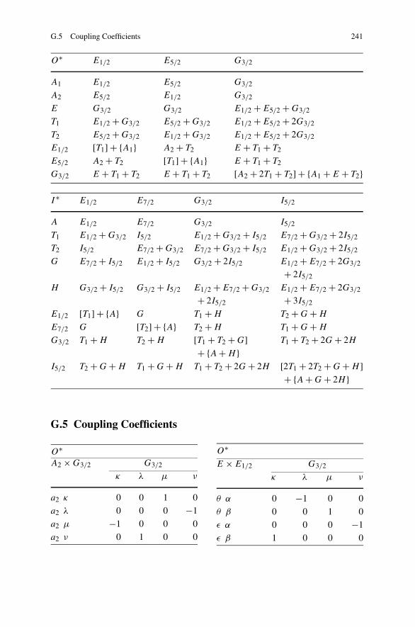
G.5 Coupling Coefficients
O∗A2 × G3/2 G3/2
κ λ μ ν
a2 κ 0 0 1 0
a2 λ 0 0 0 −1
a2 μ −1 0 0 0
a2 ν 0 1 0 0
O∗
E × E1/2 G3/2
κ λ μ ν
θ α 0 −1 0 0
θ β 0 0 1 0
ε α 0 0 0 −1
ε β 1 0 0 0
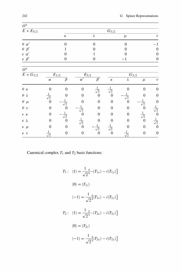
242 G Spinor Representations
O∗E × E5/2 G3/2
κ λ μ ν
θ α′ 0 0 0 −1θ β ′ 1 0 0 0ε α′ 0 1 0 0ε β ′ 0 0 −1 0
O∗E × G3/2 E1/2 E5/2 G3/2
α β α′ β ′ κ λ μ ν
θ κ 0 0 0 1√2
1√2
0 0 0
θ λ 1√2
0 0 0 0 − 1√2
0 0
θ μ 0 − 1√2
0 0 0 0 − 1√2
0
θ ν 0 0 − 1√2
0 0 0 0 1√2
ε κ 0 − 1√2
0 0 0 0 1√2
0
ε λ 0 0 1√2
0 0 0 0 1√2
ε μ 0 0 0 − 1√2
1√2
0 0 0
ε ν 1√2
0 0 0 0 1√2
0 0
Canonical complex T1 and T2 basis functions:
T1 : |1〉 = 1√2
[−|T1x〉 − i|T1y〉]
|0〉 = |T1z〉
|−1〉 = 1√2
[|T1x〉 − i|T1y〉]
T2 : |1〉 = 1√2
[−|T2x〉 − i|T2y〉]
|0〉 = |T2z〉
|−1〉 = 1√2
[|T2x〉 − i|T2y〉]
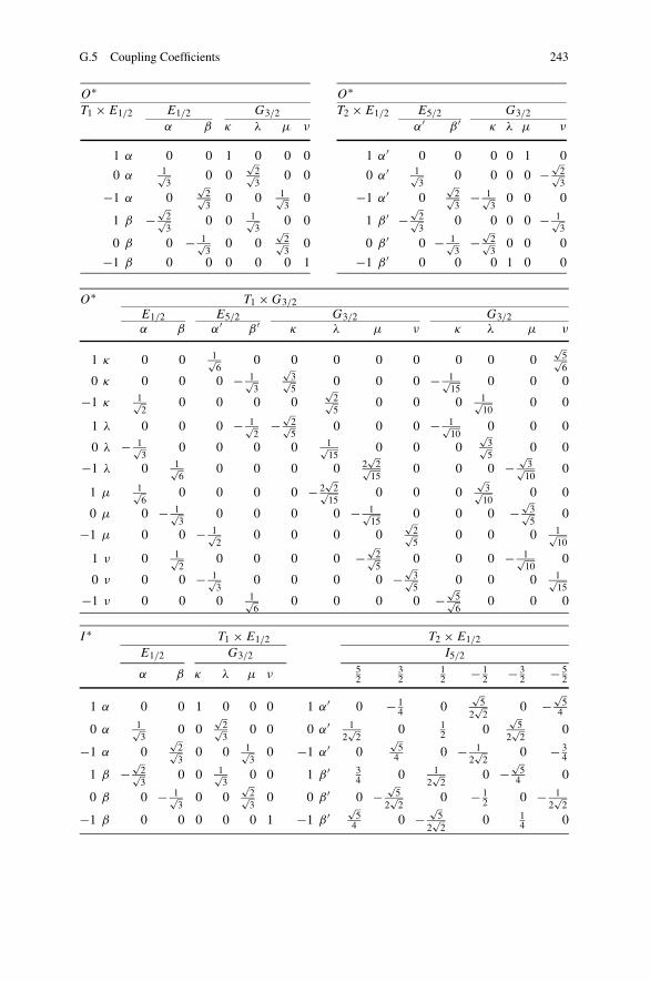
G.5 Coupling Coefficients 243
O∗T1 × E1/2 E1/2 G3/2
α β κ λ μ ν
1 α 0 0 1 0 0 0
0 α 1√3
0 0√
2√3
0 0
−1 α 0√
2√3
0 0 1√3
0
1 β −√
2√3
0 0 1√3
0 0
0 β 0 − 1√3
0 0√
2√3
0
−1 β 0 0 0 0 0 1
O∗T2 × E1/2 E5/2 G3/2
α′ β ′ κ λ μ ν
1 α′ 0 0 0 0 1 0
0 α′ 1√3
0 0 0 0 −√
2√3
−1 α′ 0√
2√3
− 1√3
0 0 0
1 β ′ −√
2√3
0 0 0 0 − 1√3
0 β ′ 0 − 1√3
−√
2√3
0 0 0
−1 β ′ 0 0 0 1 0 0
O∗ T1 × G3/2E1/2 E5/2 G3/2 G3/2α β α′ β ′ κ λ μ ν κ λ μ ν
1 κ 0 0 1√6
0 0 0 0 0 0 0 0√
5√6
0 κ 0 0 0 − 1√3
√3√5
0 0 0 − 1√15
0 0 0
−1 κ 1√2
0 0 0 0√
2√5
0 0 0 1√10
0 0
1 λ 0 0 0 − 1√2
−√
2√5
0 0 0 − 1√10
0 0 0
0 λ − 1√3
0 0 0 0 1√15
0 0 0√
3√5
0 0
−1 λ 0 1√6
0 0 0 0 2√
2√15
0 0 0 −√
3√10
0
1 μ 1√6
0 0 0 0 − 2√
2√15
0 0 0√
3√10
0 0
0 μ 0 − 1√3
0 0 0 0 − 1√15
0 0 0 −√
3√5
0
−1 μ 0 0 − 1√2
0 0 0 0√
2√5
0 0 0 1√10
1 ν 0 1√2
0 0 0 0 −√
2√5
0 0 0 − 1√10
0
0 ν 0 0 − 1√3
0 0 0 0 −√
3√5
0 0 0 1√15
−1 ν 0 0 0 1√6
0 0 0 0 −√
5√6
0 0 0
I ∗ T1 × E1/2 T2 × E1/2
E1/2 G3/2 I5/2
α β κ λ μ ν 52
32
12 − 1
2 − 32 − 5
2
1 α 0 0 1 0 0 0 1 α′ 0 − 14 0
√5
2√
20 −
√5
4
0 α 1√3
0 0√
2√3
0 0 0 α′ 12√
20 1
2 0√
52√
20
−1 α 0√
2√3
0 0 1√3
0 −1 α′ 0√
54 0 − 1
2√
20 − 3
4
1 β −√
2√3
0 0 1√3
0 0 1 β ′ 34 0 1
2√
20 −
√5
4 0
0 β 0 − 1√3
0 0√
2√3
0 0 β ′ 0 −√
52√
20 − 1
2 0 − 12√
2
−1 β 0 0 0 0 0 1 −1 β ′ √5
4 0 −√
52√
20 1
4 0
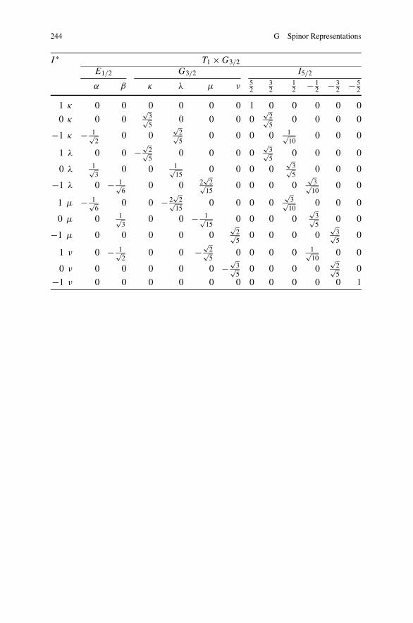
244 G Spinor Representations
I ∗ T1 × G3/2E1/2 G3/2 I5/2
α β κ λ μ ν 52
32
12 − 1
2 − 32 − 5
2
1 κ 0 0 0 0 0 0 1 0 0 0 0 0
0 κ 0 0√
3√5
0 0 0 0√
2√5
0 0 0 0
−1 κ − 1√2
0 0√
2√5
0 0 0 0 1√10
0 0 0
1 λ 0 0 −√
2√5
0 0 0 0√
3√5
0 0 0 0
0 λ 1√3
0 0 1√15
0 0 0 0√
3√5
0 0 0
−1 λ 0 − 1√6
0 0 2√
2√15
0 0 0 0√
3√10
0 0
1 μ − 1√6
0 0 − 2√
2√15
0 0 0 0√
3√10
0 0 0
0 μ 0 1√3
0 0 − 1√15
0 0 0 0√
3√5
0 0
−1 μ 0 0 0 0 0√
2√5
0 0 0 0√
3√5
0
1 ν 0 − 1√2
0 0 −√
2√5
0 0 0 0 1√10
0 0
0 ν 0 0 0 0 0 −√
3√5
0 0 0 0√
2√5
0
−1 ν 0 0 0 0 0 0 0 0 0 0 0 1
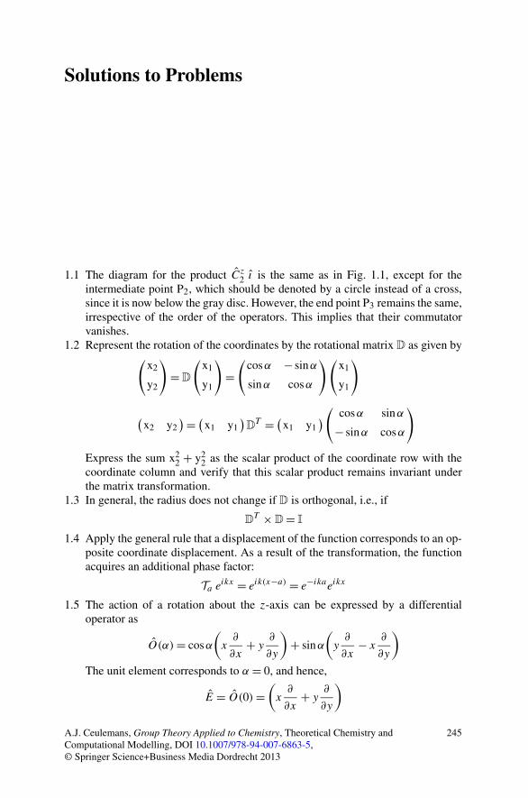
Solutions to Problems
1.1 The diagram for the product Cz2 ı is the same as in Fig. 1.1, except for the
intermediate point P2, which should be denoted by a circle instead of a cross,since it is now below the gray disc. However, the end point P3 remains the same,irrespective of the order of the operators. This implies that their commutatorvanishes.
1.2 Represent the rotation of the coordinates by the rotational matrix D as given by(x2
y2
)=D
(x1
y1
)=
(cosα − sinα
sinα cosα
)(x1
y1
)
(x2 y2
) = (x1 y1
)D
T = (x1 y1
)(cosα sinα
− sinα cosα
)
Express the sum x22 + y2
2 as the scalar product of the coordinate row with thecoordinate column and verify that this scalar product remains invariant underthe matrix transformation.
1.3 In general, the radius does not change if D is orthogonal, i.e., if
DT ×D= I
1.4 Apply the general rule that a displacement of the function corresponds to an op-posite coordinate displacement. As a result of the transformation, the functionacquires an additional phase factor:
Ta eikx = eik(x−a) = e−ikaeikx
1.5 The action of a rotation about the z-axis can be expressed by a differentialoperator as
O(α) = cosα
(x
∂
∂x+ y
∂
∂y
)+ sinα
(y
∂
∂x− x
∂
∂y
)
The unit element corresponds to α = 0, and hence,
E = O(0) =(
x∂
∂x+ y
∂
∂y
)
A.J. Ceulemans, Group Theory Applied to Chemistry, Theoretical Chemistry andComputational Modelling, DOI 10.1007/978-94-007-6863-5,© Springer Science+Business Media Dordrecht 2013
245
246 H Solutions to Problems
The angular momentum operator is given by
Lz = xpy − ypx
= �
i
(x
∂
∂y− y
∂
∂x
)
= −�
ilimα→0
O(α) − E
α
The angular momentum operator thus is proportional to an infinitesimal rotationin the neighborhood of the unit element.
2.1 The condition that C be unitary gives rise to six equations:
1 = |a|2 + |b|21 = |a|2 + |c|21 = |b|2 + |d|21 = |c|2 + |d|20 = |ac|ei(α−γ ) + |bd|ei(β−δ)
0 = |ab|ei(α−β) + |cd|ei(γ−δ)
From these equations it is clear that |a| = |d| and |b| = |c|. The phase relation-ships may be reduced to
ei(β+γ ) = −ei(α+δ)
With the help of these results the four matrix entries can be rewritten as
|a|eiα = |a|ei(α+δ)/2ei(α−δ)/2
|d|eiδ = |a|ei(α+δ)/2e−i(α−δ)/2
|b|eiβ = |b|ei(α+δ)/2ei[β− α+δ2 ]
|c|eiγ = −|b|ei(α+δ)/2ei[−β+ α+δ2 ]
The general U(2) matrix may thus be rewritten as
U= ei(α+δ)/2(
|a|ei(α−δ)/2 |b|ei[β− α+δ2 ]
−|b|ei[−β+ α+δ2 ] |a|e−i(α−δ)/2
)
with |a|2 + |b|2 = 1. Note that a general phase factor has been taken out. Theremaining matrix has determinant +1 and is called a special unitary matrix (seefurther in Chap. 7).
2.2 The relevant integrals are given by
∫ 2π
0e−ikφeikφdφ = [φ]2π
0 = 2π
∫ 2π
0e±2ikφdφ = 1
±2ik
[e±2ikφ
]2π
0 = 0
H Solutions to Problems 247
The normalized cyclic waves are thus given by
| ± k〉 = 1√2π
e±ikφ
and these waves are orthogonal: 〈−k|k〉 = 0.2.3 The combination of transposition and complex conjugation is called the adjoint
operation, indicated by a dagger. A Hermitian matrix is thus self-adjoint. Aneigenfunction of this matrix, operating in a function space, may be expressed asa linear combination
|ψm〉 =∑
k
ck|fk〉
We may arrange the expansion coefficients as a column vector c. This is calledthe eigenvector. Its adjoint, c†, is then the complex-conjugate row vector. Thecorresponding eigenvalue is denoted as Em. Now start by writing the eigenvalueequation and multiply left and right with the adjoint eigenvector:
Hc = Emc
c†Hc = Emc†c
Now take the adjoint and use the self-adjoint property of H:
c†H
†c = Emc†c
c†Hc = Emc†c
A comparison of both results shows that the eigenvalue must be equal to itscomplex conjugate and hence be real. If H is skew-symmetric, a similar argu-ment shows that the eigenvalue must be imaginary.
3.1 The table is a valid multiplication table of a group that is isomorphic to D2. Theelement C is the unit element. There are six ways to assign the three twofoldaxes to the letters A,B,D.
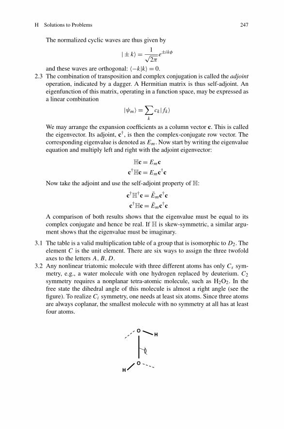
3.2 Any nonlinear triatomic molecule with three different atoms has only Cs sym-metry, e.g., a water molecule with one hydrogen replaced by deuterium. C2symmetry requires a nonplanar tetra-atomic molecule, such as H2O2. In thefree state the dihedral angle of this molecule is almost a right angle (see thefigure). To realize Ci symmetry, one needs at least six atoms. Since three atomsare always coplanar, the smallest molecule with no symmetry at all has at leastfour atoms.
248 H Solutions to Problems
3.3 There are only three regular tesselations of the plane: triangles, squares, andhexagons.
3.4 The rotation generates points that are lying on a circle, perpendicular to the ro-tation. If the rotational angle is not a rational fraction of a full angle, every timethe rotation is repeated, a new point will be generated. To obtain an integer or-der, the additional requirement is to be added that the original point is retrievedafter one full turn.
3.5 Consider a subgroup H ⊂ G such that |G|/|H | = 2. Then the coset expansionof G will be limited to only two cosets:
G = H + gH
Here g is a coset generator outside H . The subgroup is normal if the right andleft cosets coincide, Since there is only one coset outside H , it is required that
gH = Hg
Suppose that this equation does not hold. Then this can only mean that there areelements in H such that
hx g = hy
But then the coset generator must be an element of H , which contradicts thestaring assumption.
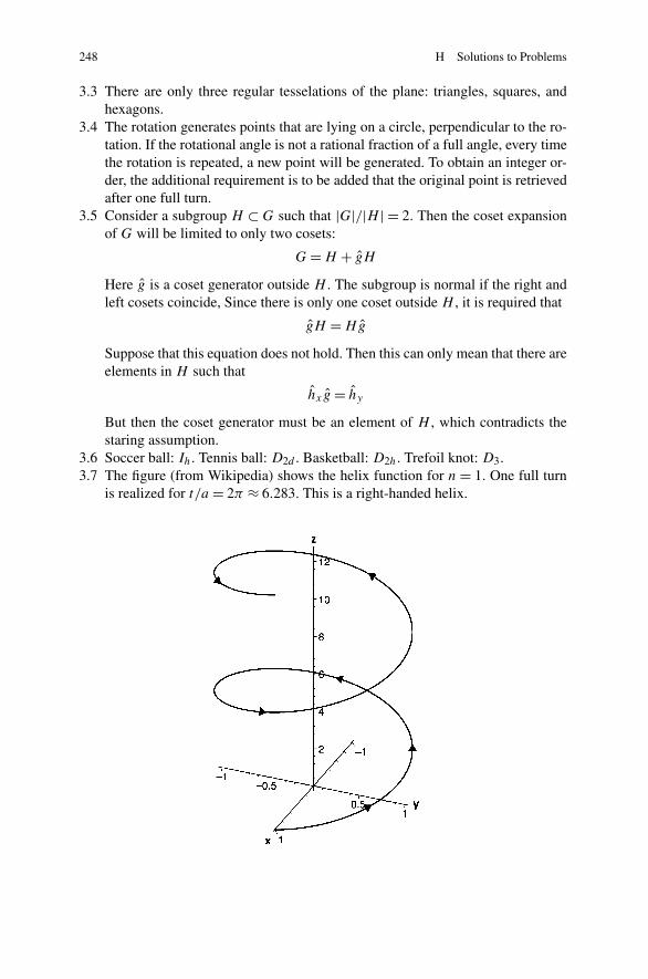
3.6 Soccer ball: Ih. Tennis ball: D2d . Basketball: D2h. Trefoil knot: D3.3.7 The figure (from Wikipedia) shows the helix function for n = 1. One full turn
is realized for t/a = 2π ≈ 6.283. This is a right-handed helix.
H Solutions to Problems 249
The enantiomeric function reads:
x(t) = a cos
(nt
a
)
y(t) = a sin
(−nt
a
)
z(t) = t
Note that a uniform sign change of t would leave the right-handed helix un-changed. For the discrete helix, the screw symmetry consists of a translation inthe z-direction over a distance 2πa/m in combination with a rotation aroundthe z-axis over an angle 2πn/m. If m is irrational, the helix will not be periodic,and the screw symmetry is lost.
4.1 The site symmetry of a cube is Th. The cube is an invariant of its site groupand transforms as ag in Th. The set of five cubes thus spans the induced rep-resentation: aTh ↑ Ih. Applying the Frobenius theorem to the subduction (seeSect. C.1), one obtains
aTh ↑ Ih = Ag + Gg (1)
4.2 The irreps can be obtained from the induction table in Sect. C.2, as ΓπC3v ↑ Td :
ΓπC3v ↑ Td = E + T1 + T2 (2)
The SALCs shown span the tetrahedral E irrep, the one on the left is theEθ component, and the one on the right is the Eε component. Note that theytransform into each other by rotating all π -orbitals over 90◦ in the same sense[13].
4.3 The 24 carbon atoms of coronene form three orbits: two orbits of six atoms,corresponding to the internal hexagon and to the six atoms on the outer ringthat have bonds to the inner ring, and one orbit of the twelve remaining atoms.The elements of the 6-orbit occupy sites of C′
2v symmetry, based on C′2, σh, σv
in D6h. The pz orbitals on these sites transform as b1, and hence the inducedirreps are as in the case of benzene:
b1C2v ↑ D6h = B2g + A2u + E1g + E2u (3)
The remaining 12-orbit connects carbon atoms with only Cs site symmetry,the pz orbitals on these sites transforming as a′′. The induced irreps read:
a′′Cs ↑ D6h = B1g + B2g + A1u + A2u + 2E1g + 2E2u (4)
The A1u and B1g irreps only appear in the 12-orbit, so we can infer that themolecular orbitals with this symmetry will entirely be localized on the 12-orbit. The SALCs can easily be constructed, as they should be antisymmetricwith respect to the σv planes in order not to hybridize with the SALCs basedon the 6-orbits.
250 H Solutions to Problems
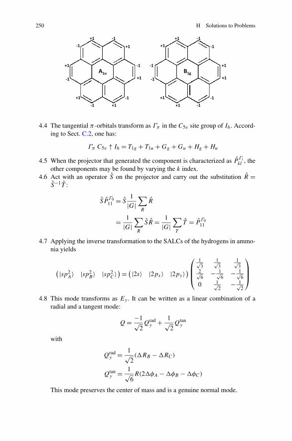
4.4 The tangential π -orbitals transform as Γπ in the C5v site group of Ih. Accord-ing to Sect. C.2, one has:
Γπ C5v ↑ Ih = T1g + T1u + Gg + Gu + Hg + Hu
4.5 When the projector that generated the component is characterized as PΓi
kl , theother components may be found by varying the k index.
4.6 Act with an operator S on the projector and carry out the substitution R =S−1T :
SPΓ011 = S
1
|G|∑R
R
= 1
|G|∑R
SR = 1
|G|∑T
T = PΓ011
4.7 Applying the inverse transformation to the SALCs of the hydrogens in ammo-nia yields
( |sp2A〉 |sp2
B〉 |sp2C〉) = ( |2s〉 |2px〉 |2py〉
)⎛⎜⎜⎝
1√3
1√3
1√3
2√6
− 1√6
− 1√6
0 1√2
− 1√2
⎞⎟⎟⎠
4.8 This mode transforms as Ey . It can be written as a linear combination of aradial and a tangent mode:
Q = −1√2Qrad
y + 1√2Qtan
y
with
Qrady = 1√
2(RB − RC)
Qtany = 1√
6R(2φA − φB − φC)
This mode preserves the center of mass and is a genuine normal mode.
H Solutions to Problems 251
4.9 Since all irreps are one-dimensional, the characters can only consist of a phasefactor:
D(C5) = eiλI (5)
The fifth power of the generator will yield the unit element, and hence,
e5iλ = 1 (6)
This is the Euler equation. Its solutions are the characters in the table of C5,as given in Appendix A.
4.10 The product of inversion with a C2 axis must yield a reflection plane, per-pendicular to this axis. As an example, a product of type ı · C′
2 must yield areflection plane of σd type, as this is perpendicular to the primed twofold axis.For the one-dimensional irreps of D6h, one thus should have
χ(ı)χ(C′
2
) = χ(σd) (7)
This is indeed verified to be the case.4.11 The a′′
2 distortion is antisymmetric with respect to 3C2, σh, and 2S3. As aresult, when the mode is launched, all these symmetry elements will be de-stroyed, and the symmetry reduces to the subgroup C3v . In general, the resultof a distortion will always be the maximal subgroup for which the distortionis totally symmetric [14].
4.12 The group of this fullerene is D6d . The 24 atoms separate into two orbits: a 12-orbit containing the top and bottom hexagons and another 12-orbit containingthe crown of the 12 atoms, numbered from 7 to 18. In both cases the site groupis only Cs , and hence both orbits will span the same irreps:
a′Cs ↑ D6d = A1 + B2 + E1 + E2 + E3 + E4 + E5
Quite remarkably, the Hückel spectrum for this fullerene has a nonbondinglevel of E4 symmetry.
5.1 Let ri and rj denote the position vectors of electrons i and j . The electronrepulsion operator contains the distance between both electrons as |ri −rj |. Thematrix D(R) expresses the transformation of the Cartesian coordinates under arotation. This matrix will also rotate the coordinate differences:
R
⎛⎝xi − xj
yi − yj
zi − zj
⎞⎠ = D(R)
⎛⎝xi − xj
yi − yj
zi − zj
⎞⎠ (8)
Exactly as in the derivation for Problem 1.2, the square of the distance betweenthe two electrons is then found to be invariant under any orthogonal transfor-mation of the coordinates.
5.2 For the G irrep, it is noted from Sect. C.1 that a tetrahedral splitting field willbranch G into A + T . It thus acts as a splitting field to isolate the unique Ga
component. Symmetry adaptation to Cz2 will yield two totally symmetric com-
ponents, one of which will be the Ga already obtained; the remaining one is
252 H Solutions to Problems
then Gz. The corresponding Gx and Gy may then be found by cyclic permuta-tion under the C
xyz
3 axis.
For the H irrep, one may make use of the Cxyz
3 axis again. It resolves H
into A1 + 2E. This unique A1 component will be the sum Hξ +Hη +Hζ . Wecan project the Hζ component out of this sum by using the Cz
2 axis. Althoughthe H level subduces three totally symmetric irreps in C2, there will be nocontamination with Hθ and Hε since these were already removed in the firststep by projecting out the trigonal A1.
5.3 The total number of nuclear permutations and permutation-inversions forCH3BF2 is 24. This is the product of six permutations of the protons, twopermutations of the fluorine nuclei, and the binary group of the spatial inver-sion. However, as the fluxionality of this molecule is limited to free rotationsof the methyl group, the operations should be limited to those permutationsor permutation-inversions that lead to structures that can be rotated back tothe original frame or to a rotamer of this frame. Only half of the operationswill comply with this requirement. As an example, the odd permutations of theprotons are not allowed since the resulting structure cannot be turned into theoriginal one by outer rotations or by rotations of the methyl group around theC-B bond. The results are given in [15]. The corresponding symmetry group isisomorphic with D3h.
5.4 Ferrocene is a molecule with two identical coaxial rotors. Its nuclear permu-tation-inversion group consists of 100 elements. It has a halving rotational sub-group of 50 proper permutations: for each of the cyclo-pentadienyl rings, thereare 5 cyclic permutation operations, yielding a total of 52 = 25 operations, andthis number must be doubled to account for the permutation of the upper andlower rings. In addition, there is a coset of improper permutation-inversionscontaining the other 50 elements. This coset also contains two kinds of ele-ments. In the table we summarize the structure of the group. The carbon atomsare numbered 1, . . . ,5 in the upper ring and 6, . . . ,10 in the lower ring.
Nuclear permutation-inversion group for ferrocene (u and l refer to upperand lower rotor)
R #
Cu5 × Cl
5 (12345) 25(ul) (16) (2,10) (39) (48) (57) 255σ u
v × 5σ lv (25) (34) (7,10) (89)∗ 25
(ul)∗ (16) (27) (38) (49) (5,10)∗ 25
6.1 The (t1u)2 configuration gives rise to 15 states. The direct product decomposes
as follows (see Appendix D):
T1u × T1u = [A1g + Eg + T2g] + {T1g}The symmetrized part will give rise to six singlet functions, while there arenine triplet substates, forming a 3T1g multiplet. Since the 3-electron Ψ state is a
H Solutions to Problems 253
quartet, the singlet states cannot contribute, and we need to couple the triplet toa 2T1u state, resulting from a (t1u)
1 configuration. The orbital part of the tripletis obtained from the T1 × T1 = T1 coupling table in Appendix F:
|T1gx〉 = 1√2
[−y(1)z(2) + z(1)y(2)]
|T1gy〉 = 1√2
[x(1)z(2) − z(1)x(2)
]
|T1gz〉 = 1√2
[−x(1)y(2) + y(1)x(2)]
The coupling with the third electron can yield A1u, Eu, T1u, and T2u states. Ourresults is based on the A1u product. This yields
A1u = 1√3
[|T1gx〉|x(3)〉 + |T1gy〉|y(3)〉 + |T1gz〉|z(3)〉]
= − 1√6
∣∣∣∣∣∣∣∣
x(1) y(1) z(1)
x(2) y(2) z(2)
x(3) y(3) z(3)
∣∣∣∣∣∣∣∣This should be multiplied by the product of the three α-spins, α1α2α3, to obtainthe 4A1u ground state of the (t1u)
3 configuration.6.2 The JT problem is determined by the symmetrized direct product of T1u. As we
have seen in the previous problem, this product contains A1g +Eg +T2g . SinceA1g modes do not break the symmetry, the JT problem is of type T1 ×(e+ t2). Inthe linear problem only two force elements are required. The distortion matrixis thus as follows:
H′ = FE√6
⎛⎜⎜⎝
Qθ 0 0
0 Qθ 0
0 0 −2Qθ
⎞⎟⎟⎠ + FT√
2
⎛⎜⎜⎝
0 −Qζ −Qη
−Qζ 0 −Qξ
−Qη 0ξ 0
⎞⎟⎟⎠
6.3 The magnetic dipole operator transforms as T1g , while the direct square of eg
irreps yields A1g + A2g + Eg . Since the operator irrep is not contained in theproduct space, the selection rules will not allow a dipole matrix element be-tween eg orbitals.
6.4 We first draw a simple diagram representing the R-conformation. The pointgroup is C2. The twofold-axis is oriented along the y-direction, and the centersof the two chromophores are placed on the positive and negative x-axes. Thedipole moments are then oriented as
μ1 = μ
(0, cos
α
2,− sin
α
2
)
μ2 = μ
(0, cos
α
2, sin
α
2
)
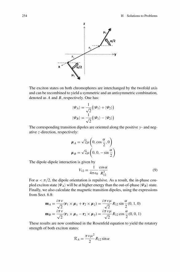
254 H Solutions to Problems
The exciton states on both chromophores are interchanged by the twofold axisand can be recombined to yield a symmetric and an antisymmetric combination,denoted as A and B , respectively. One has:
|ΨA〉 = 1√2
(|Ψ1〉 + |Ψ2〉)
|ΨB〉 = 1√2
(|Ψ1〉 − |Ψ2〉)
The corresponding transition dipoles are oriented along the positive y- and neg-ative z-direction, respectively:
μA = √2μ
(0, cos
α
2,0
)
μB = √2μ
(0,0,− sin
α
2
)
The dipole-dipole interaction is given by
V12 = 1
4πε0
cosα
R312
(9)
For α < π/2, the dipole orientation is repulsive. As a result, the in-phase cou-pled exciton state |ΨA〉 will be at higher energy than the out-of-phase |ΨB〉 state.Finally, we also calculate the magnetic transition dipoles, using the expressionsfrom Sect. 6.8:
mA = iπν√2
(r1 × μ1 + r2 × μ2) = iπνμ√2
R12 sinα
2(0,1,0)
mB = iπν√2
(r1 × μ1 − r2 × μ2) = iπνμ√2
R12 cosα
2(0,0,1)
These results are now combined in the Rosenfeld equation to yield the rotatorystrength of both exciton states:
RA = πνμ2
2R12 sinα
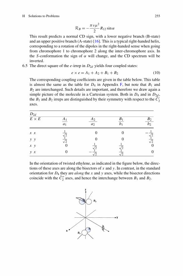
H Solutions to Problems 255
RB = −πνμ2
2R12 sinα
This result predicts a normal CD sign, with a lower negative branch (B-state)and an upper positive branch (A-state) [16]. This is a typical right-handed helix,corresponding to a rotation of the dipoles in the right-handed sense when goingfrom chromophore 1 to chromophore 2 along the inter-chromophore axis. Inthe S-conformation the sign of α will change, and the CD spectrum will beinverted.
6.5 The direct square of the e-irrep in D2d yields four coupled states:
e × e = A1 + A2 + B1 + B2 (10)
The corresponding coupling coefficients are given in the table below. This tableis almost the same as the table for D4 in Appendix F, but note that B1 andB2 are interchanged. Such details are important, and therefore we draw again asimple picture of the molecule in a Cartesian system. Both in D4 and in D2d ,the B1 and B2 irreps are distinguished by their symmetry with respect to the C′
2axes.
D2d
E × E A1 A2 B1 B2a1 a2 b1 b2
x x 1√2
0 0 − 1√2
y y 1√2
0 0 1√2
x y 0 1√2
1√2
0
y x 0 − 1√2
1√2
0
In the orientation of twisted ethylene, as indicated in the figure below, the direc-tions of these axes are along the bisectors of x and y. In contrast, in the standardorientation for D4 they are along the x and y axes, while the bisector directionscoincide with the C′′
2 axes, and hence the interchange between B1 and B2.
256 H Solutions to Problems
Note that the two-electron states are symmetrized, except the A2 combination.The symmetrized states will combine with singlet spin states, while the A2 statewill be a triplet. One thus has:
1A1 = 1√2
(x(1)x(2) + y(1)y(2)
) 1√2
(α(1)β(2) − β(1)α(2)
)
= 1√2
(∣∣(xα)(xβ)∣∣ + ∣∣(yα)(yβ)
∣∣)
1B1 = 1√2
(∣∣(xα)(yβ)∣∣ + ∣∣(yα)(xβ)
∣∣)
1B2 = 1√2
(−∣∣(xα)(xβ)∣∣ + ∣∣(yα)(yβ)
∣∣)
3A2 = ∣∣(xα)(yα)∣∣
The 1A1 and 1B2 states are the zwitterionic states, while the 1B1 and 3A2 statesare called the diradical states. It is clear from the expressions that in both casesthe two radical carbon sites are neutral. The zwitterionic states are easily polar-izable though.
6.6 The carbon atoms form two orbits. The pz orbital on the central atom is inthe center of the symmetry group and transforms as a′′
2 . The three methyleneorbitals are in C2v sites, transforming as the b2 irrep of the site group, i.e., theyare antisymmetric with respect to σh and symmetric with respect to σv . Theinduced representation is
b2C2v ↑ D3h = a′′2 + e′′ (11)
The SALCs are entirely similar to the hydrogen SALCs in the case of am-monia; this implies, for instance, that the component labeled x is symmetricunder the vertical symmetry plane through atom A. It will be antisymmetricfor the twofold-axis going through atom A since the relevant orbital is of pz
type:
|Ψa〉 = 1√3
(|pA〉 + |pB〉 + |pC〉)
|Ψx〉 = 1√6
(2|pA〉 − |pB〉 − |pC〉)
|Ψy〉 = 1√2
(|pB〉 − |pC〉)
The a′′2 orbitals interact to yield bonding and antibonding combinations at
E = α ± √3β . Since the graph is bipartite, the remaining e′′ orbitals are neces-
H Solutions to Problems 257
sarily nonbonding and will be occupied by two electrons. The direct square ofthis irrep yields symmetrized A′
1 and E′ states and an antisymmetrized A′2 state.
The expressions for these states are obtained from the coupling coefficients forD3 in Appendix F:
1A′1 = 1√
2
(x(1)x(2) + y(1)y(2)
) 1√2
(α(1)β(2) − β(1)α(2)
)
= 1√2
(∣∣(xα)(xβ)∣∣ + ∣∣(yα)(yβ)
∣∣)
1E′x = 1√
2
(∣∣(xα)(yβ)∣∣ + ∣∣(yα)(xβ)
∣∣)
1E′y = 1√
2
(−∣∣(xα)(xβ)∣∣ + ∣∣(yα)(yβ)
∣∣)
3A2 = ∣∣(xα)(yα)∣∣
Note that the distinction between zwitterionic and diradical states does nothold in this case. Formally, TMM can be described as a valence isomer be-tween three configurations in which one of the peripheral atoms has a dou-ble bond to the central atom and the other two sites carry an unpaired elec-tron.
7.1 In a cube the d-shell also splits in eg + t2g , but the ordering is reversed. Explicitcalculation of the potential shows that the splitting is reduced by a factor 8/9:
cube = −8
9octahhedron
7.2 Perform the matrix multiplication and verify that the product matrix is ofCayley–Klein form. The multiplication is not commutative:
(a1 b1
−b1 a1
)×
(a2 b2
−b2 a2
)=
(a1a2 − b1b2 a1b2 + a2b1
−a1b2 − a2b1 a1a2 − b1b2
)(12)
7.3 The double group D∗3 contains 12 elements. In Table 7.5 we have listed the six
representation matrices for the elements on the positive hemisphere. The CA2
axis is along the x-direction, CB2 is at −60◦ and CC
2 is at +60◦. The derivationof the multiplication table and the underlying class structure (see Table 7.6) isbased on a straightforward matrix multiplication.
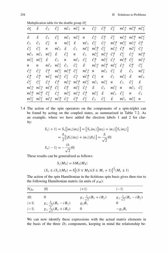
258 H Solutions to Problems
Multiplication table for the double group D∗3
D∗3 E C3 C2
3 ℵC3 ℵC23 ℵ CA
2 CB2 CC
2 ℵCA2 ℵCB
2 ℵCC2
E E C3 C23 ℵC3 ℵC2
3 ℵ CA2 CB
2 CC2 ℵCA
2 ℵCB2 ℵCC
2
C3 C3 C23 ℵ ℵC2
3 E ℵC3 CC2 CA
2 ℵCB2 ℵCC
2 ℵCA2 CB
2
C23 C2
3 ℵ ℵC3 E C3 ℵC23 ℵCB
2 CC2 ℵCA
2 CB2 ℵCC
2 CA2
ℵC3 ℵC3 ℵC23 E C2
3 ℵ C3 ℵCC2 ℵCA
2 CB2 CC
2 CA2 ℵCB
2
ℵC23 ℵC2
3 E C3 ℵ ℵC3 C23 CB
2 ℵCC2 CA
2 ℵCB2 CC
2 ℵCA2
ℵ ℵ ℵC3 ℵC23 C3 C2
3 E ℵCA2 ℵCB
2 ℵCC2 CA
2 CB2 CC
2
CA2 CA
2 CB2 ℵCC
2 ℵCB2 CC
2 ℵCA2 ℵ ℵC3 C2
3 E C3 ℵC23
CB2 CB
2 ℵCC2 ℵCA
2 CC2 CA
2 ℵCB2 C2
3 ℵ C3 ℵC23 E ℵC3
CC2 CC
2 CA2 CB
2 ℵCA2 ℵCB
2 ℵCC2 ℵC3 ℵC2
3 ℵ C3 C23 E
ℵCA2 ℵCA
2 ℵCB2 CC
2 CB2 ℵCC
2 CA2 E C3 ℵC2
3 ℵ ℵC3 C23
ℵCB2 ℵCB
2 CC2 CA
2 ℵCC2 ℵCA
2 CB2 ℵC2
3 E ℵC3 C23 ℵ C3
ℵCC2 ℵCC
2 ℵCA2 ℵCB
2 CA2 CB
2 CC2 C3 C2
3 E ℵC3 ℵC23 ℵ
7.4 The action of the spin operators on the components of a spin-triplet canbe found by acting on the coupled states, as summarized in Table 7.2. Asan example, where we have added the electron labels 1 and 2 for clar-ity:
Sx | + 1〉 = Sx
[|α1〉|α2〉] = [
Sx |α1〉]|α2〉 + |α1〉
[Sx |α2〉
]= �
2
[|β1〉|α2〉 + |α1〉|β2〉] = �√
2|0〉
Sy | − 1〉 = − i�√2|0〉
These results can be generalized as follows:
Sz|MS〉 = �MS |MS〉(Sx ± iSy)|MS〉 = �
[(S ∓ MS)(S ± Ms + 1)
] 12 |Ms ± 1〉
The action of the spin Hamiltonian in the fictitious spin basis gives then rise tothe following Hamiltonian matrix (in units of μB ):
HZe |0〉 |+1〉 |−1〉〈0| 0 g⊥ 1√
2(Bx + iBy) g⊥ 1√
2(Bx − iBy)
〈+1| g⊥ 1√2(Bx − iBy) g||Bz 0
〈−1| g⊥ 1√2(Bx + iBy) 0 −g||Bz
We can now identify these expressions with the actual matrix elements inthe basis of the three D3 components, keeping in mind the relationship be-
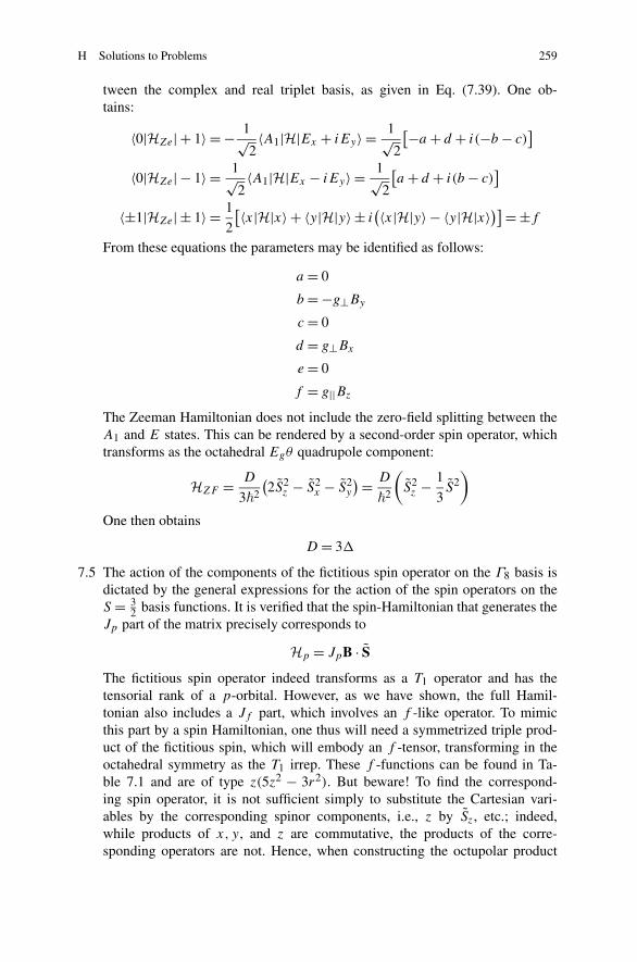
H Solutions to Problems 259
tween the complex and real triplet basis, as given in Eq. (7.39). One ob-tains:
〈0|HZe| + 1〉 = − 1√2〈A1|H|Ex + iEy〉 = 1√
2
[−a + d + i(−b − c)]
〈0|HZe| − 1〉 = 1√2〈A1|H|Ex − iEy〉 = 1√
2
[a + d + i(b − c)
]
〈±1|HZe| ± 1〉 = 1
2
[〈x|H|x〉 + 〈y|H|y〉 ± i(〈x|H|y〉 − 〈y|H|x〉)] = ±f
From these equations the parameters may be identified as follows:
a = 0
b = −g⊥By
c = 0
d = g⊥Bx
e = 0
f = g||Bz
The Zeeman Hamiltonian does not include the zero-field splitting between theA1 and E states. This can be rendered by a second-order spin operator, whichtransforms as the octahedral Egθ quadrupole component:
HZF = D
3�2
(2S2
z − S2x − S2
y
) = D
�2
(S2
z − 1
3S2
)
One then obtains
D = 3
7.5 The action of the components of the fictitious spin operator on the Γ8 basis isdictated by the general expressions for the action of the spin operators on theS = 3
2 basis functions. It is verified that the spin-Hamiltonian that generates theJp part of the matrix precisely corresponds to
Hp = JpB · S
The fictitious spin operator indeed transforms as a T1 operator and has thetensorial rank of a p-orbital. However, as we have shown, the full Hamil-tonian also includes a Jf part, which involves an f -like operator. To mimicthis part by a spin Hamiltonian, one thus will need a symmetrized triple prod-uct of the fictitious spin, which will embody an f -tensor, transforming in theoctahedral symmetry as the T1 irrep. These f -functions can be found in Ta-ble 7.1 and are of type z(5z2 − 3r2). But beware! To find the correspond-ing spin operator, it is not sufficient simply to substitute the Cartesian vari-ables by the corresponding spinor components, i.e., z by Sz, etc.; indeed,while products of x, y, and z are commutative, the products of the corre-sponding operators are not. Hence, when constructing the octupolar product
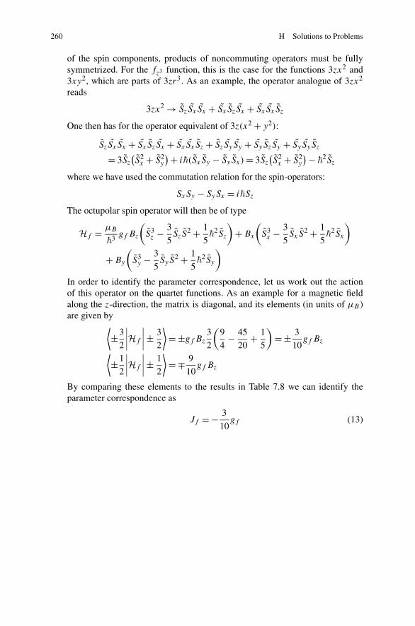
260 H Solutions to Problems
of the spin components, products of noncommuting operators must be fullysymmetrized. For the fz3 function, this is the case for the functions 3zx2 and3xy2, which are parts of 3zr3. As an example, the operator analogue of 3zx2
reads
3zx2 → SzSx Sx + Sx SzSx + Sx Sx Sz
One then has for the operator equivalent of 3z(x2 + y2):
SzSx Sx + Sx SzSx + Sx Sx Sz + SzSy Sy + Sy SzSy + Sy Sy Sz
= 3Sz
(S2
x + S2y
) + i�(Sx Sy − Sy Sx) = 3Sz
(S2
x + S2y
) − �2Sz
where we have used the commutation relation for the spin-operators:
SxSy − SySx = i�Sz
The octupolar spin operator will then be of type
Hf = μB
�3gf Bz
(S3
z − 3
5SzS
2 + 1
5�
2Sz
)+ Bx
(S3
x − 3
5Sx S
2 + 1
5�
2Sx
)
+ By
(S3
y − 3
5Sy S
2 + 1
5�
2Sy
)
In order to identify the parameter correspondence, let us work out the actionof this operator on the quartet functions. As an example for a magnetic fieldalong the z-direction, the matrix is diagonal, and its elements (in units of μB )are given by⟨
±3
2
∣∣∣∣Hf
∣∣∣∣ ± 3
2
⟩= ±gf Bz
3
2
(9
4− 45
20+ 1
5
)= ± 3
10gf Bz
⟨±1
2
∣∣∣∣Hf
∣∣∣∣ ± 1
2
⟩= ∓ 9
10gf Bz
By comparing these elements to the results in Table 7.8 we can identify theparameter correspondence as
Jf = − 3
10gf (13)
References
1. Mulliken, R.S., Ramsay, D.A., Hinze, J. (eds.): Selected Papers. University of Chicago Press,Chicago (1975)
2. Cotton, F.A.: Chemical Applications of Group Theory. Wiley, New York (1963)3. Atkins, P.W., Child, M.S., Phillips, C.S.G.: Tables for Group Theory. Oxford University Press,
Oxford (1970)4. Boyle, L.L.: The method of ascent in symmetry. I. Theory and tables. Acta Cryst. A 28, 172
(1972)5. Fowler, P.W., Quinn, C.M.: Theor. Chim. Acta 70, 333 (1986)6. Griffith, J.S.: The Theory of Transition-Metal Ions. Cambridge University Press, Cambridge
(1961)7. Boyle, L.L., Parker, Y.M.: Symmetry coordinates and vibration frequencies for an icosahedral
cage. Mol. Phys. 39, 95 (1980)8. Qiu, Q.C., Ceulemans, A.: Icosahedral symmetry adaptation of |JM〉 bases. Mol. Phys. 100,
255 (2002)9. Butler, P.H.: Point Group Symmetry Applications, Methods and Tables. Plenum Press, New
York (1981)10. Herzberg, G.: Molecular Spectra and Molecular Structure. III. Electronic Spectra and Elec-
tronic Structure of Polyatomic Molecules. Van Nostrand, Princeton (1966)11. Fowler, P.W., Ceulemans, A.: Symmetry relations in the property surfaces of icosahedral
molecules. Mol. Phys. 54, 767 (1985)12. Fowler, P.W., Ceulemans, A.: Spin-orbit coupling coefficients for icosahedral molecules.
Theor. Chim. Acta 86, 315 (1993)13. Stone, A.J.: A new approach to bonding in transition-metal clusters. Theory. Mol. Phys. 41,
1339 (1980)14. Ceulemans, A., Vanquickenborne, L.G.: The epikernel principle. Structure and Bonding 71,
125–159 (1989)15. Longuet-Higgins, H.C.: The symmetry group of non-rigid molecules. Mol. Phys. 6, 445
(1963)16. Kobayashi, N., Higashi, R., Titeca, B.C., Lamote, F., Ceulemans, A.: Substituent-induced cir-
cular dichroism in phthalocyanines. J. Am. Chem. Soc. 121, 12018 (1999)
A.J. Ceulemans, Group Theory Applied to Chemistry, Theoretical Chemistry andComputational Modelling, DOI 10.1007/978-94-007-6863-5,© Springer Science+Business Media Dordrecht 2013
261
Index
Symbols10Dq , 168, 169-enantiomer, 138, 139�8 quartet, 184, 190π -modes, 78σ -mode, 78
AAbel, 27Abelian, 27, 32, 41, 47, 56, 62Abragam, 182, 190Absorption spectra, 144acac−, 138Aldridge, 84, 101Allene, 46Alternant, 97Altmann, ix, 16, 19, 72, 101, 164, 190Ammonia, 21–24, 28–30, 32, 34, 36, 39, 43,
52, 53, 55, 56, 59, 68, 72, 75, 76, 103,104, 110–112, 250, 256
AmmoniaDynamic symmetry, 110–112Permutation symmetry, 28–30, 36Point group, 21–24, 32, 34, 43, 72, 104SALC, 52–56, 59, 68, 75, 76, 250
Angular momentum, 10, 89, 133, 134, 146,165, 185, 188, 190, 246
Annulene, 87Antiprisms, 40, 43Antisymmetrization, 119, 121, 123, 125, 183,
219, 257Archimedean solids, 93Archimedene, 102Aromaticity, 87Associativity, 24Atkins, 191, 261Atomic population, 85
Automorphism group, 27, 92, 95, 98Azimuthal coordinate, 165
BBalabanov, 134, 161Barut, viiBarycentre rule, 146, 169, 170, 186Basis set, canonical, 65, 107, 217Bending modes, 65, 83Benfey, 36Benzene, 41, 42, 85, 87, 99, 249Bernoulli, 5Berry, 5Berry phase, 10Bersuker, ix, 128, 134, 161Bethe, 176, 179, 235Beyens, ix, 121, 160Biel, 149, 161Bilinear interaction, 135, 136, 172Binary elements, 180Bipy, 138, 140, 144, 161Bisphenoid, 41Bleaney, 182, 190Boggs, 134, 161Bohr magneton, 89Bond order, 85Born-Oppenheimer condition, 110–112Boundary condition, 110Boundary operation, 152Boyle, ix, 39, 49, 211, 215, 218, 261Bra function, 116, 173Bracket, 5, 8, 11, 12, 58, 67, 68, 114, 117, 126,
183Branching rule, 218Braun, ix, 144, 161Bruns, 93Buckminsterfullerene, 38–40, 49, 157, 158
A.J. Ceulemans, Group Theory Applied to Chemistry, Theoretical Chemistry andComputational Modelling, DOI 10.1007/978-94-007-6863-5,© Springer Science+Business Media Dordrecht 2013
263
264 Index
Bunker, 110, 112Butler, 117, 160, 165, 190, 218, 261
CC60, 38–40, 49, 102, 157, 158, 190Calabrese, 40, 49Cauchy theorem, 154Cayley, 26, 27, 29, 171–173, 176, 178, 179,
189, 257graph, 26, 27, 93theorem, 29, 173
Cayley–Klein parameters, 171–173, 176, 178,257
Centrosymmetry, 45Ceulemans, 72, 93, 121, 139, 149, 152, 157,
170, 188Character, 17, 40, 56–62, 64, 69, 70, 75–77,
84, 115, 119, 128, 135, 140, 152, 165,167, 169, 179, 235
string, 58, 60–62, 64, 70, 115, 135table, 57–60, 62, 64, 70, 100, 116,
176–178, 235theorem, 51, 58, 63, 70, 75, 78, 115, 116,
120, 152, 178, 179Charge-transfer (CT) transitions, 139Chatterjee, 149Chemical bonding, 153Chemical shift, 91Chibotaru, ix, 93, 102Child, 191, 261Chirality, 21, 46Chromophore, 138, 147, 255Circular dichroism, 46, 113, 138, 139, 141,
143–145, 147, 159, 161, 261Circular polarization, 19, 46, 113, 132, 138,
144, 145, 152, 153, 158, 159Clar, 157–159Class, 32–34, 45, 57–59, 62, 64, 70, 71, 75, 93,
102, 178–180, 189, 257Clebsch-Gordan (CG) coefficient, 117, 118,
121, 122, 128, 183Closed shell, 87, 143Closure, 24, 33, 61, 69, 136, 137Clusters, 101, 113, 161, 261Commutator, 8, 133, 147, 245Compernolle, ix, 170, 190Condon, 174Condon–Shortley convention, 174Cone, 43, 44Conical intersection, 132Conjugation, 32, 158
class, 32complex, 14–17, 118, 121, 167, 180, 181,
183, 247
Conrotatory, 136, 137Contact term, 140, 144Continuity condition, 175Coordinate system, 10, 38, 78, 138, 139, 141,
145, 147Cartesian, 10, 38, 138D2 setting, 217tetragonal, 93–95, 108, 131–133trigonal, 37
Coordination compounds, 37Coset, 30–33, 45, 71–73, 248, 252Cotton, 191, 261Coulomb interaction, 109Coulson, 84, 97, 101, 102Coulson–Rushbrooke theorem, 97Coupling channel, 128Coupling coefficients, 117–119, 121, 122, 124,
128, 130, 131, 135, 139, 142, 143, 159,168, 173, 174, 183, 185, 186, 221–235,241, 243, 255, 257, 261
exchange symmetry, 122Crystal-field potential, 169Crystallography, 40Cube, 35, 37, 39, 54, 93, 99, 150, 169, 170,
189, 249, 257Cuboctahedron, 170Curie principle, 104, 105Curl, 38, 49Cvetkovic, 84Cyclobutene, 136Cyclohexadiene, 137Cylinder, 34, 40–43
DDay, 139Day and Sanders model, 139, 140Degeneracy, 56, 62, 70, 98, 100, 102, 103, 105,
106, 128, 132, 161, 180–183Deltahedron, 154, 157Determinant, 15, 16, 45, 54, 83, 125, 126, 159,
164, 171, 172, 246unimodular, 171
Diatomic, 43Dihedral, 40, 62, 159, 194, 247Dipole, 7, 89, 103–105, 113, 127, 139–145,
159, 186, 253, 254induced, 104moment, 89, 103–105, 127, 140, 144, 159
Dirac, 11Dirac notation, 11, 67, 133Direct square, 119–121, 129, 165, 177, 184,
188, 253, 255, 257Dish, 102
Index 265
Dish Archimedene, 93Disrotatory, 137Dissymmetry, 104Distortion modes, 130, 133Dodecahedrane, 38, 49Dodecahedron, 35, 36, 38, 39, 99, 156, 157,
170Domcke, 132, 161Donor–acceptor interactions, 139, 140Doob, 84Double group, 176–178, 180, 184, 189, 235,
257, 258Dual, 7, 10, 35, 39, 153, 154, 156, 157, 170Dynamic symmetry, 111, 112
EEdge representation, 151–156Edmonds, 165, 190Eigenfunctions, 53–56, 61, 81, 85, 89, 90, 97,
103, 105–107, 124, 132, 161Eigenvalues, 19, 54, 81, 83, 84, 86, 87, 91, 94,
97, 102, 105, 107, 108, 188, 189Electric, 7, 21, 43, 46, 47, 69, 104, 113, 127,
146, 148, 153, 205, 206see Stark effectcrystal field, 69dipole, 7, 104, 113, 127field (E), 42, 47, 96, 151–155, 158, 159symmetry breaking, 69, 205, 206
Electron diffraction, 83Electron precise, 155Enantiomers, 160Equivalent electrons, 124, 125Euclid, 39Euler equation, 54, 150, 251Euler theorem, 113, 152, 161Excited state, 41, 135, 145, 148Exciton, 145, 146, 148, 160, 254
FFace representation, 151Fagan, 40, 49Faraday effect, 2, 46Ferrocene, 40, 41, 112, 252Fibre bundle, 148, 149, 157, 158Flint, 134Fowler, ix, 93, 102, 152, 156, 157, 161, 211,
221, 235, 261Franck-Condon principle, 144Fries, 157–159Frobenius, 56, 72, 76, 93, 148, 249Frontier orbitals, 138, 156, 157Fullerenes, 156, 157, 159, 161, 190
Function space, 7, 10, 12–16, 23, 51–53,55–57, 59–61, 63, 64, 66–68, 71, 78,82, 93, 97, 106, 113, 114, 134, 149,163, 165–167, 170, 181, 182, 184, 247
GGauge, 51, 88–90Genealogical tree, 29, 30, 36, 69GFP protein, 43Gilmore, 165, 190Graph, 26, 27, 36, 84, 92, 95–98, 256
automorphism, 26, 27, 92, 95, 98bipartite, 97, 98, 256
Great Orthogonality Theorem (GOT), 63Griffith, 106, 112, 117, 160, 175, 184, 185,
190, 215, 218, 221, 235, 261Group
see Lie groupssee point groupsAbelian, 27alternating, 28, 36, 40, 152cyclic, 27, 28, 31, 39, 41, 42, 44, 62, 86,
87, 100, 108, 165, 181, 252definition, 1, 28, 32, 98, 108, 109, 111,
128, 176double, 19, 40, 62, 126, 175–180, 184, 189,
190, 235, 257, 258generator, 27, 30, 39, 41, 45, 63, 107, 123halving, 45, 48, 164, 252orthogonal, 35, 63, 163, 164, 172permutation, 25, 28, 29, 73, 108–112, 123,
126, 148, 165, 252symmetric, 27, 29, 36, 42, 55, 58, 62, 76,
93, 100, 104, 123, 148, 150–152, 165,177, 247, 251, 256
unitary, 57, 58, 163, 171
HHaake, 180, 190Halevi, 136, 161Half-integral momentum, 134Hamiltonian, 8, 17, 18, 53, 84, 85, 89, 92, 103,
105–110, 113, 129, 131, 133–135, 141,147, 170, 171, 173–175, 181–190, 258,259
Heath, 38, 49Helicity, 138, 144Hemisphere, 176, 179, 257Hermitian, 19, 170, 183, 247Hessian, 80, 81, 83, 84Hexadecapole, ix, 168, 169Hilbert space, 8, 53Hilton, 152, 161Hoffmann, 136, 155HOMO, 98, 160
266 Index
Homomorphism, 11, 14, 172, 173, 175Hückel theory, 84, 87, 106Hydrocarbon, 85, 95, 97
IIcosahedron, 35, 38–40, 154, 170, 217Indistinguishability, 110, 123Induction, 32, 51, 69, 71–76, 78, 93, 96, 99,
148–150, 158, 207, 208, 210–214, 249Integral, 12, 84, 114, 115, 127, 134
hopping, 84overlap, 114, 115, 127resonance, 84
Intensity, 140, 143, 144, 148Intra-ligand (IL) transitions, 138, 144, 145, 147Inversion, 2, 17, 18, 34, 40, 42, 44–47, 61, 62,
109–112, 167, 180, 251, 252Irrep, see representation, irreducibleIsolobal analogy, 155Isomorphism, 28, 172Isotope shift, 83
JJahn, 128Jahn–Teller effect, 70, 128Judd, ix, 134, 161
KKatzir, 103, 112Kinetic energy, 80, 88, 89, 109Klein, 27, 171–173, 176, 178, 179, 189, 257
see Cayleyfour-group, 27
Kobayashi, ix, 44, 49, 261Köppel, 132Kramers’ degeneracy, 106Kronecker delta, 12, 13, 65Kroto, 38, 49
LLagrange theorem, 31Lagrangian, 80Lanthanides, 69Le Bel, 36Leapfrog, 156, 157, 159Lie groups, 165, 190
SO(3), O(3), 35, 163, 164, 167, 172, 173,175, 204, 210, 237
SU(2), U(2), 171–173, 175, 179, 189, 246Ligand orbitals, 140, 144, 145Ligator, 138–140Lijnen, ix, 121, 160, 170, 190Linear dichroism, 138, 139, 161Linearly polarized, 46Lipscomb, 38, 48
London, 88London approximation, 89Longuet-Higgins, 109–112, 261Lulek, ix, 149, 161LUMO, 98, 158
MMagnetic, 21, 41, 42, 46, 47, 63, 69, 87–91,
104, 110, 113, 127, 146–148, 153, 159,170, 173, 180, 181, 184, 187–189, 205,206, 253, 254, 260
see Faradaysee Londondipole, 89, 113, 127, 159, 253, 254field (B), 47flux, 91symmetry breaking, 41, 69, 205, 206
Mallion, ix, 84, 97, 101, 102Malone, 40, 49Manifold, 100, 124, 125, 135, 168, 188Manolopoulos, 156Martins, 170Mass-weighted coordinates, 80, 82Matrix, 3, 4, 6, 7, 10–16, 19, 22, 23, 45, 51–54,
56, 59, 60, 63, 65, 73–75, 77, 80, 81,83–85, 90, 92, 97, 98, 106–108, 114,115, 126, 127, 129, 131, 135, 159, 164,165, 167, 170–175, 179, 180, 182,186–189, 245–247, 251, 253, 257–260
adjacency, 84, 85circulant, 85complex conjugate, 13, 14, 16, 63, 171,
173, 174diagonalization, 54, 84element, 14, 22, 23, 54, 59, 64, 73, 74,
83–85, 92, 108, 115, 116, 126–132,135, 137, 140, 142, 143, 147, 164, 172,173, 175, 183, 253
orthogonal, 16, 19, 63, 163, 172, 245, 247trace, 59, 60, 64, 83, 115, 127, 167, 170transposed, 10, 16, 171unitary, 11, 14–16, 19, 57, 107, 127, 163,
171, 179, 181, 246Matsuda, 44, 49M(CO)3 fragments, 155Melvin, 149, 161Methane, 76Mexican hat potential, 131, 132Mingos, 156, 161Miura, 93, 102Molecular-symmetry group, 109Monopole, 153Mulliken, 62Mulliken symbols, 62, 191
Index 267
Multiplication table, 22–29, 31, 47, 177, 189,247, 257, 258
Mys, 188, 190
NNeumann principle, 104Nordén, 138Normal modes, 81, 100, 129, 250
OO’Brien, 38, 49OCAMS, 161Octahedron, 35, 37, 70, 95, 96, 107, 138, 148,
149, 154, 159, 168, 170, 187–189, 216Octupole, 186Odabasi, 174Ojha, 95, 102O’Leary, 84, 101Omnicapping, 101, 157Opechowski, 178Opechowski theorem, 178Operator
action on a function, 4, 51, 52, 181action on a point, 1action on an operator, 1, 66anti-linear, 11congruence, 46idempotent, 69inverse, 18, 23, 171inversion, 2, 17, 18, 109, 110, 112ladder, 65, 67, 108, 112linear, 11–13, 16–18, 53, 105, 114, 133,
146, 147, 180, 188, 253projection, 65, 67, 86, 100proper and improper, vii, 163, 165rotation, 2, 8–10, 16, 23, 53, 86, 112, 133,
134, 176, 180, 245, 246, 251rotation-reflection, 40spin, 125, 134, 170, 173, 180, 181,
184–186, 188–190, 259, 260Orbitals, 4–7, 11, 23, 41, 51–53, 55, 59, 60,
63, 76–78, 84–89, 94, 95, 98–101, 107,108, 115, 117, 123, 136–145, 149,155–157, 159–161, 165, 168, 169, 204,211, 249, 250, 253, 256
d, 78, 95, 107, 108, 165, 168, 204f, 78, 149molecular, 4, 51, 77, 84, 85, 95, 98, 99,
101, 149, 156, 161, 211, 249Order of a group, 32, 33, 59, 114Organo–transition–metal complexes, 78, 107,
138Orgel, 138, 161Orthonormality, 15, 16, 116, 118, 135Orthorhombic, 34, 40, 71, 131–133
PPaquette, 38, 49Parity
permutational, 28, 36, 110, 118space, 167, 182
Parker, 215, 218, 261Partial derivative, 129Partitioning, 30, 31Pauli exclusion principle, 125Pauling, 77Pekker, 134, 161Permutation group, 126, 165Perturbation theory, 135Phase convention, 108, 167Phillips, 191, 261Platonic solids, 34–36, 153, 154, 170Point groups, 34–37, 39, 41–45, 47, 62, 117,
121, 181, 192C2, Ci , Cs , 27, 29, 30, 34, 39, 45–47, 72,
75, 94, 104, 192, 205, 206, 211–214,247, 249, 251–253
C3v , 44, 62Cn, Cnh, Cnv , 27, 41, 43, 44, 62, 72, 76,
90, 95, 151, 192, 195, 196, 206D2, 27, 176, 208, 211, 217, 218, 247D2h, 34, 38, 39D6h, 41, 42, 87, 100, 199, 212, 249, 251Dn, Dnd , Dnh, 40, 45, 90, 194, 198, 199,
206I , Ih, 35, 36, 39, 40, 93, 99, 120, 205, 209,
210, 214, 218, 237, 248–250O , Oh, 35–37, 39, 70–72, 78, 93–98, 116,
118, 122, 149, 184, 185, 205, 209, 210,214
S2n, 42, 62T , Td , Th, 35–40, 45, 47, 62, 76, 99,
150–152, 181, 205, 208, 209, 213, 220,249
Polarization function, 149Polyhedrane, 155Polyhedron, 48, 93, 99, 148, 150–154, 248Potential energy, 80, 89, 110Prisms, 40, 43Product
antisymmetrized, 119, 121, 125, 219direct group, 45, 46, 176direct representation, 125multiplicity, 121, 128, 184scalar, 10–12, 14, 58, 59, 63, 80, 115, 118,
127, 128, 154, 174, 245symmetrized, 120, 121, 125, 177, 184, 219,
252, 253, 259, 260Pseudo Jahn–Teller effect (PJT), 134, 136, 137Pseudo-doublet, 188
268 Index
Pseudo-scalar representation, 152Pythagorean tradition, 35
QQiu, ix, 218, 261Quantum chemistry, vii, 8, 103, 104, 106, 108,
110, 112, 149Quartet spin state, 184, 188Quinn, 211, 261
RRank, 168, 259Reciprocity theorem, 72, 93, 148Reduced matrix element, 127, 128, 142, 173Representation
determinantal, 126faithful, 23, 175ground, 72–74, 126irreducible, 55–59, 62, 63, 65, 68, 106, 107mechanical, 148, 149, 154, 155, 211positional, 73, 74, 148–150, 211pseudoscalar, 152, 153, 156
Reversal, 11, 16–18, 63, 91, 109, 110, 129,180–184
space, 18, 63, 109, 110, 181–183time, 11, 16–18, 63, 91, 110, 129, 180–184
Rhombohedral, 168, 169, 189Right-thumb rule, 90Ring closure, 136, 137Rodger, 138, 161Rodrigues, 174Rosenfeld equation, 254Rotation, 1–10, 16, 22, 23, 32, 34, 40–45, 48,
52, 53, 61, 78, 83, 86, 87, 90, 95, 107,109, 111, 112, 133, 134, 139, 151–154,163, 164, 167, 172, 175, 176, 179, 180,189, 197, 235, 245, 246, 248, 249, 251,255
bodily, 52, 61, 111, 112matrix, 3, 6, 7, 10, 16, 23, 45, 52, 53, 83,
163–165, 167, 172, 175, 179, 180, 245,251
operator, 2, 8–10, 16, 23, 53, 86, 112, 133,134, 176, 180, 245, 246, 251
optical, 36pole, 2, 3, 164, 175, 176
Rotatory strength, 148, 254Rouvray, 97, 102Ru(bipy)3, 144Ruthenocene, 40, 41
SSachs, 84SALC, 53, 55, 59, 65, 67, 76, 77, 86, 152
Salem, 84, 101Samuel, 93, 102Sanders, 139Satten, 189, 190Schäffer, 39Schrödinger
stationary equation, 17, 106time-dependent equation, 17
Schulman, 93, 102Schur, 56, 61, 63, 107Secular equation, 54, 81, 132, 186
see ZeemanSelection rule, 65, 115, 128–130, 135, 137,
142Shapere, 5, 134Shimanouchi, 81, 101Similarity transformation, 32, 72Singleton, 40, 62Site symmetry, 75, 76, 93, 94, 148, 149, 249Smalley, 38, 49sp3-hybridization, 76, 77, 150Spherical harmonics, 165–168, 218Spin, spinor, 170, 171, 173–175, 177, 180,
183–185, 259Spin-orbit coupling, 175, 186, 235, 261Splitting scheme, 71, 121Stabilizer, 30, 33, 39, 72Standard fibre, 149Stanger, 93, 102Stark effect, 46Stereo-isomers, 70Stone, 261Stretching modes, 82, 83Subduction, 29, 51, 69–73, 75, 87, 165, 167,
168, 184, 207–210, 212, 214, 218, 237,249
Subelement, 73–75Subgroup, 29–34, 36–40, 43, 45–48, 69–72,
101, 128, 164, 176, 248, 251, 252Subporphyrin, 44Subrepresentation, 65, 68, 126Sum rule, 75, 136, 148Symmetry
see operatorssee point groupsactive definition, 1, 7, 10, 22, 46, 130, 132breaking, 30, 34, 41, 69, 70, 128, 136, 205,
206dynamic, 41, 111, 112hidden, 95, 98, 106spherical, 34, 35, 40, 117, 149, 163–166,
168, 170, 172, 174, 176, 178, 180, 182,184, 186, 188, 190, 204, 205
Index 269
TTakeuchi, 44, 49Tangential modes, 78Teller, 128Tetragonal compression, 133Tetragonal elongation, 132Tetrahedron, 35–37, 76, 77, 99, 150–152, 154Tight-binding model, 84Time reversal, 11, 16–18, 63, 180–183Time-even, time-odd, 181, 182Topology, 150Trace, 57, 59–61, 64, 68, 83, 109, 115, 119,
120, 127, 165–167, 170Transfer term, 140–144Transition dipole, 140, 144Translation, 10, 17, 18, 36, 43, 48, 78, 82, 109,
154, 158, 249Triangular condition, 128Triphenylmethyl, 95–98, 106Trischelate complex, 177Trivalent polyhedron, 93, 154Troullier, 170Truncation, 157Twisted cylinder, 43Two-well potential, 132
UUni-axial, 43Unit element, 14, 22, 24, 27–30, 32, 38, 44, 59,
61, 69, 152, 164, 172, 175, 176,245–247, 251
Uranium, 78, 80, 83
VVanquickenborne, ix, 139, 161, 261
Van’t Hoff, 36Vector, 3, 7, 10–15, 41, 43, 52–54, 60, 63, 77,
79, 80, 87–90, 104, 106, 140, 142, 146,163–165, 170–176, 247
axial, 41polar, 43, 104potential, 80, 87–89, 146row versus column, 7, 10, 14, 53, 63, 247
Vertex representation, 150Vibrational modes, 81, 131, 149Vibronic interaction, 160Vollhardt, 93, 102
WWalçerz, 188Wales, 156, 161Walsh diagram, 3, 132, 165Wigner, 17, 19, 113, 117, 126–129, 135, 136,
140, 142, 160, 173, 181, 185, 190Wigner–Eckart theorem, 113, 126–129, 135,
136, 140, 173, 185Wilczek, 5, 134Woodward–Hoffmann rule, 136Wunderlich, 38Wylie, 152
YYarkony, 132Yersin, 144Yu-De, 81Yun-Guang, 81
ZZeeman interaction, 170, 182, 186
Related Documents