CHAPTERS FOUR AND FIVE: DEMAND (OR KNOWING YOUR CUSTOMER) Demand Function – The relation between demand and factors influencing its level. Quantity of.

CHAPTERS FOUR AND FIVE: DEMAND (OR KNOWING YOUR CUSTOMER)

Demand Function – The relation between demand and factors influencing its level.

Quantity of product X demanded = Qx =

f(Price of X, Prices of Related Goods, Consumer Income, Advertising Expenditure, etc.)

THE MARKET DEMAND FUNCTION, CONT.

The model:

Qx = a0 + a1Px + a2Pz + a3Y + a4POP + a5i + a6AD + e

The terms a0 , a1 , etc. are the parameters of the model.

This is what we need to estimate.

Estimation of the model:

Q = 100 + -.002Px + .001Pz + .00008Y + .22POP + -800i + .002A

Interpretation of the model:

If the average price increases by $1, the demand for the product falls by .002 units

THE DEMAND CURVE

Demand Curve – The relation between price and the quantity demanded, holding all else constant.

General Form: P = a – bQ Why is this the general form?

Moving from the Demand Function to the Demand Curve.

CONNECTING THE CURVE TO THE FUNCTION

Changes in quantity demanded – movement along a given demand curve reflecting a change in price and quantity.

Shift in demand – Switch from one demand curve to another following a change in a non-price determinant of demand

IF AN INDEPENDENT VARIABLE CHANGES, OTHER THAN PRICE OF THE GOOD, YOU MUST DRAW A NEW DEMAND CURVE!!!

Demand Analysis and Estimation: Discussion

Outline• Demand Sensitivity Analysis:

Elasticity

• Price Elasticity of Demand

• Cross Price Elasticity of Demand

• Income Elasticity of Demand

• Additional Demand Elasticity Concepts

Demand Sensitivity Analysis: Elasticity

• Elasticity – The percentage change in a dependent variable resulting from a 1% change in an independent variable.

• Elasticity = % change in Y / % change in X

• ELASTICITY IS A RATIO!!!

Percentage Change Elasticity = Percentage Change in Quantity (Sales) / Percentage Change in (X) Percentage change = (X2-X1)/X1

Price Elasticity of Demand

Price Elasticity of Demand (Own-Price):◦ Measure of the magnitude by which consumers alter the

quantity of some product they purchase in response to a change in the price of that product.

◦ Responsiveness of the quantity demanded to changes in the price of the product, holding constant the values of all other variables in the demand function.

Estimating from the Demand Function. Estimating from the Demand Curve.

The Point Formula

((Q2-Q1)/Q1) / ((P2-P1)/P1)

Problems:1. Order of events dictate outcomes2. Does not impose ceteris paribus.

The Arc Formula

((Q2-Q1)/(Avg.Q) / ((P2-P1)/(Avg.P)

Problem:

1. Does not impose ceteris paribus

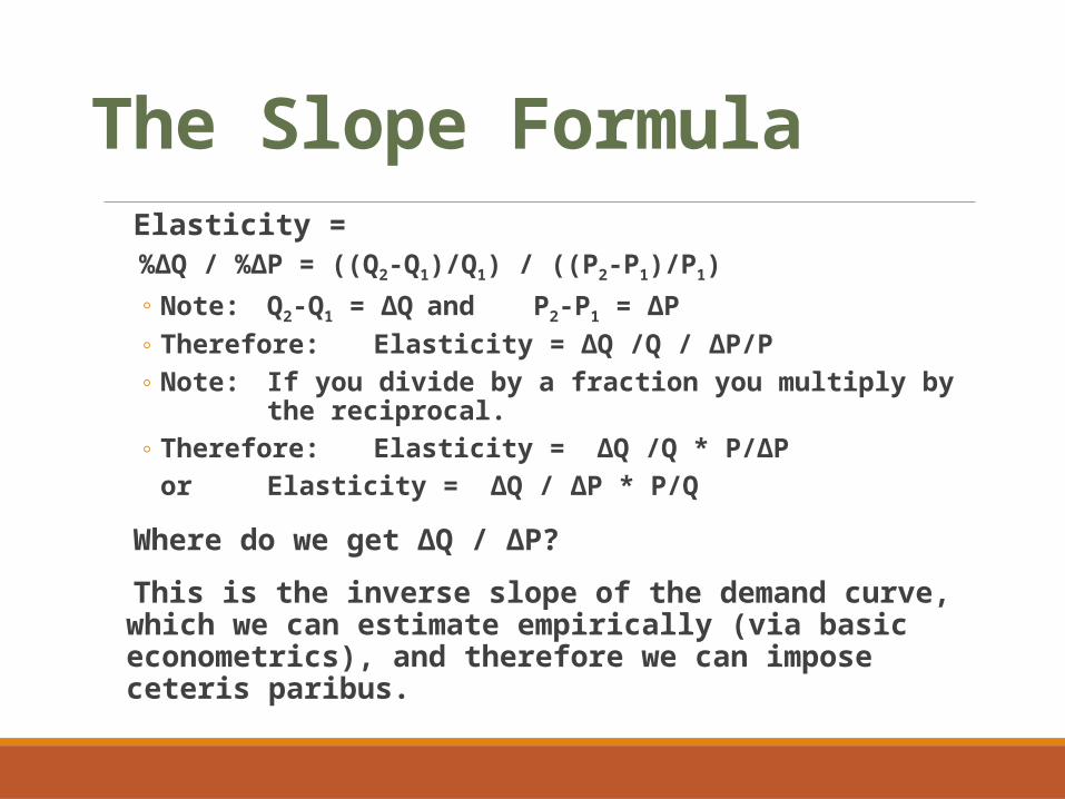
The Slope Formula Elasticity =

%ΔQ / %ΔP = ((Q2-Q1)/Q1) / ((P2-P1)/P1)◦ Note: Q2-Q1 = ΔQ and P2-P1 = ΔP◦ Therefore: Elasticity = ΔQ /Q / ΔP/P◦ Note: If you divide by a fraction you multiply by the

reciprocal.◦ Therefore: Elasticity = ΔQ /Q * P/ΔP

or Elasticity = ΔQ / ΔP * P/Q

Where do we get ΔQ / ΔP?

This is the inverse slope of the demand curve, which we can estimate empirically (via basic econometrics), and therefore we can impose ceteris paribus.

Interpretation of Price Elasticity

% change in Q > % change in P ◦ (elastic or responsive) Ep > 1

% change in Q < % change in P ◦ (inelastic or unresponsive) Ep < 1

% change in Q = % change in P ◦ (unitary elastic) Ep = 1

Own Price Elasticity and the Demand Curve

Own-price elasticity = %ΔQ / %ΔP

How does elasticity vary along a linear demand curve?

The upper half of a linear demand curve is elastic.

The lower half of a linear demand curve is inelastic.

BE ABLE TO EXPLAIN WHY!!!◦ The search for substitutes as price increases◦ Big number, small number explanation◦ Calculating elasticity at the midpoint.

Pric

e

$10

9

8

7

65

4

32

1

0 1 2 3 4 5 6 7 8 9 10 Quantity

Elasticity Along a Demand Curve

Elasticity declines along demand curve as we move toward the quantity axis

Ed =

Ed = 1

Ed = 0

Ed < 1

Ed > 1

Elasticity and Total Revenue Connecting Elasticity to Total Revenue If % change in Q > % change in P

decreasing the price will increase TR

and marginal revenue must be positive. If % change in Q < % change in P

increasing the price will increase TR

and marginal revenue must be negative. BE ABLE TO ILLUSTRATE THE RELATIONSHIP

Marginal Revenue Marginal Revenue - amount of revenue from the last unit sold.◦ the rate of change in total revenue◦ the slope of the total revenue curve.

If demand is downward sloping, then price will exceed marginal revenue. In other words, the amount of revenue generated by an additional sale will be less than the price the firm charges.

Why? To increase quantity the firm will need to lower the price, not just for the last unit sold, but also for every unit the firm wishes to sell.

Profit and Elasticity Profit = Total Revenue - Total Cost

If demand is inelastic (i.e. % change in Q < % change in P) an increase in price will increase TR.

Because Q falls (law of demand), so too will Total Cost

Why? Total Cost (which we will discuss later) is an increasing function of output. The more you produce, the higher your total cost.

Consequently, if demand is inelastic, a firm can raise its price and increase its profits.

Summarizing Demand

The Law of Demand - Quantity demanded rises as price falls, ceteris paribus. Quantity demanded falls as price rises, ceteris paribus

◦ The Law of Demand is based upon Gossen’s First and Second Laws.◦ The Law of Demand gives us the Demand Curve◦ Via own-price elasticity, we move from the demand curve to total revenue.

Total Revenue = Price * Quantity◦ Without own-price elasticity we do not know how changes in price and

quantity will impact total revenue.◦ The variation in total revenue gives us the concept of marginal revenue.

Optimal Pricing Policy

MR = P [1 + 1/EP] Be able to show why this relationship

exists. To maximize profits: MR = MC MC = P [1+1/EP]

P = MC / [1 + 1/EP]

Lerner Index

Lerner Index (Measure of Inequality)

L = (p - MC)/p Lerner Index is bound between

(0,1) Closer to 1 the more pricing power

the firm has. NOTE: Mark-up power reflects

monopoly power.

The Lerner Index Own Price Elasticity is Always

Negative. MR = P[1 – 1/EP] and therefore MC = P[1 – 1/EP] or MC = P - P/EP or P – MC = P/ EP or [P-MC]/P = 1/EP PUNCHLINE: If elasticity

increases, mark-up will decline. If the product becomes less elastic, mark-up will increase.

Determinants of Price Elasticity The extent the good is considered a necessity. Proportion of income spent on the product Time Availability of substitutes HINT: The fourth determinant encompasses the

first three. PUNCHLINE: The key to establishing market

power is the elimination of substitutes in the minds of consumers.

WHAT IMPACT DOES ADVERTISING HAVE ON ELATICITY?

Cross Price Elasticity of DemandSubstitutes vs. Complements

• Substitutes – products for which a price increase for one leads to an increase in demand for the other. • NOTE: Two goods are substitutes only if the consumer

behavior indicates this relationship.• Complements – products for which a price increase

for one leads to a decrease in demand for the other.

Cross- Price Elasticity

• Responsiveness of demand for one product to changes in the price of another.

• Calculating from the Demand Function• Note: We already know if two goods are

substitutes or complements from the demand function. We do not know the magnitude of the relationship without calculating elasticity.

Income ElasticityNormal vs. Inferior Goods

• Normal Goods – products for which demand is positively related to income.

• Inferior Goods – products for which demand is negatively related to income.

• Note: What is normal or inferior can vary across time and geographic distance.

Income Elasticity

• Responsiveness of demand to changes in income.• Calculating from the Demand Function• Note: We already know if two goods are normal or

inferior from the demand function. We do not know the magnitude of the relationship without calculating elasticity.

Income Elasticity and the Business Cycle

• Counter-cyclical goods – inferior goods• During recessions demand will increase.• During expansion demand will decrease.

• Non-cyclical normal goods – income elasticity is less than 1.

• Cyclical normal goods – superior goods – luxury goods – income elasticity is greater than 1.

Additional Demand Elasticity Concepts

• Advertising Elasticity• Interest Rate Elasticity• Weather Elasticity• Any factor that can be included

in a demand function can be analyzed in terms of elasticity.

SHORT-RUN AND LONG-RUN ELASTICITIES OF DEMAND

Price elasticityProduct Short Run Long Run

Tobacco products 0.46 1.89Electicity (household) 0.13 1.89Health Services 0.20 0.92Nodurable toys 0.30 1.02Movies/motion pictures 0.87 3.67Beer 0.56 1.39Wine 0.68 0.84University tuition 0.52 —

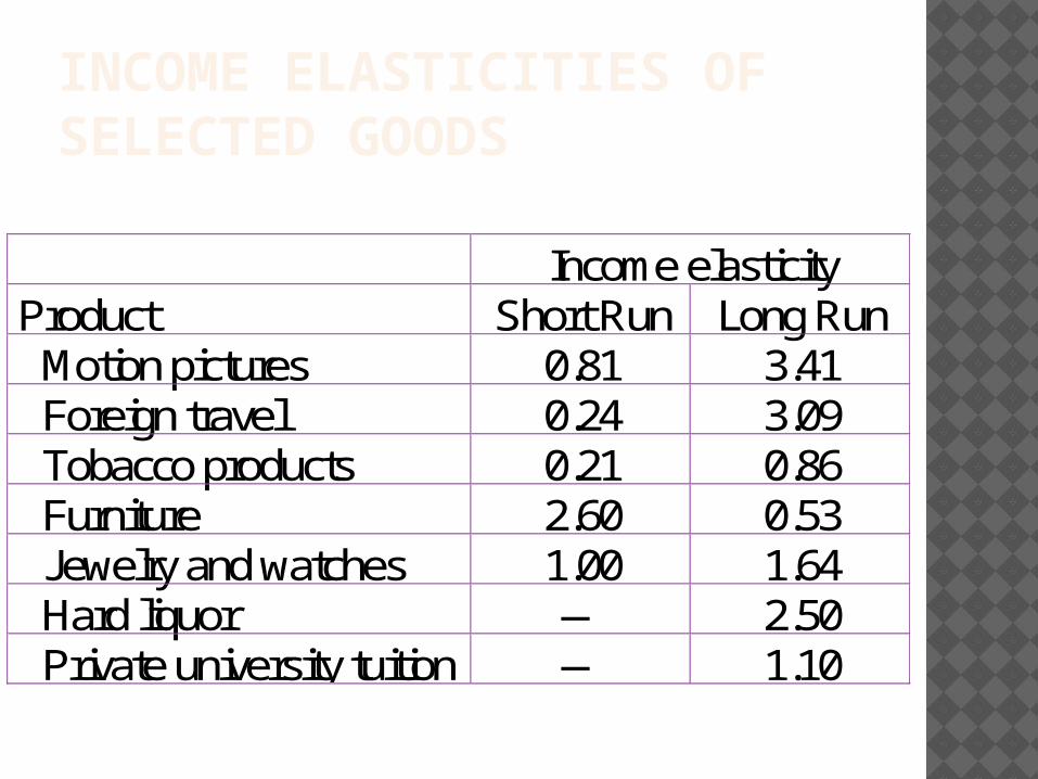
INCOME ELASTICITIES OF SELECTED GOODS

Income elasticityProduct Short Run Long Run

Motion pictures 0.81 3.41Foreign travel 0.24 3.09Tobacco products 0.21 0.86Furniture 2.60 0.53Jewelry and watches 1.00 1.64Hard liquor — 2.50Private university tuition — 1.10

CROSS-PRICE ELASTICITIES

CommoditiesCross-Price

ElasticityBeef in response to price change in pork 0.11Beef in response to price change in chicken 0.02U.S. automobiles in response to price changes

in European and Asian automobiles 0.28European automobiles in response to price

changes in U.S. and Asian automobiles 0.61Beer in response to changes in wine 0.23Hard liquor in response to price changes in

beer - 0.11

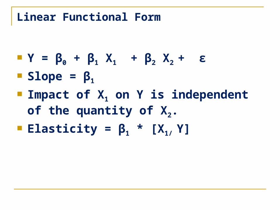
Linear Functional Form

Y = β0 + β1 X1 + β2 X2 + ε Slope = β1 Impact of X1 on Y is independent of

the quantity of X2. Elasticity = β1 * [X1/ Y]

Double-Log Functional Form

What if you wished to estimate the following model?

Y = β0 X1 β1 X2β2

To make this linear in the parameters

InY = β0 + β1 InX1 + β2 InX2 + ε Slope = β1 = ΔlnY / ΔlnX1 = [ΔY / Y] / [ΔX1 /

X1] What is this? The elasticity, which

is constant across the sample.

What is the slope in a double log functional form?

Slope = β1 * (Y/X) =

[ΔY / Y] / [ΔX1 / X1] * (Y/X) =

ΔY / ΔX Impact of X1 on Y depends upon the

quantity of X2

In other words, the slope of X1

varies across the sample. Why would this be a realistic

property?