TIME-DEPENDENT PROBLEMS The previous three chapters dealt exclusively with steady- state problems, that is, problems where time did not enter explicitly into the formulation or solution of the problem. The types of problems considered in Chapters 2 and 3, respectively, were one- and two-dimensional elliptic boundary value problems. In this chapter, finite element models for parabolic and hyperbolic equations, such as the one-dimensional transient heat conduction and the one-dimensional scalar wave equation, respectively, will be developed. TIME-DEPENDENT PROBLEMS The finite element models for these two types of initial- boundary value problems will turn out to be, respectively, first- and second-order systems of ordinary differential equations with time as the independent variable. Analytical and numerical algorithms for the solution of these systems of equations will be presented and discussed. TIME-DEPENDENT PROBLEMS The finite element models for these two types of initial- boundary value problems will turn out to be, respectively, first- and second-order systems of ordinary differential equations with time as the independent variable. Analytical and numerical algorithms for the solution of these systems of equations will be presented and discussed. TIME-DEPENDENT PROBLEMS The finite element models for these two types of initial- boundary value problems will turn out to be, respectively, first- and second-order systems of ordinary differential equations with time as the independent variable. Analytical and numerical algorithms for the solution of these systems of equations will be presented and discussed. TIME-DEPENDENT PROBLEMS The finite element models for these two types of initial- boundary value problems will turn out to be, respectively, first- and second-order systems of ordinary differential equations with time as the independent variable. Analytical and numerical algorithms for the solution of these systems of equations will be presented and discussed. TIME-DEPENDENT PROBLEMS One-Dimensional Diffusion or Parabolic Equations The example to be used to develop a model for one- dimensional diffusion processes is the classical heat conduction problem shown below: Insulated Insulated CIVL 7/8111 Time-Dependent Problems - 1-D Diffusion Equation 1/21

Welcome message from author
This document is posted to help you gain knowledge. Please leave a comment to let me know what you think about it! Share it to your friends and learn new things together.
Transcript
TIME-DEPENDENT PROBLEMS
The previous three chapters dealt exclusively with steady-state problems, that is, problems where time did not enter explicitly into the formulation or solution of the problem.
The types of problems considered in Chapters 2 and 3, respectively, were one- and two-dimensional elliptic boundary value problems.
In this chapter, finite element models for parabolic and hyperbolic equations, such as the one-dimensional transient heat conduction and the one-dimensional scalar wave equation, respectively, will be developed.
TIME-DEPENDENT PROBLEMS
The finite element models for these two types of initial-boundary value problems will turn out to be, respectively, first- and second-order systems of ordinary differential equations with time as the independent variable.
Analytical and numerical algorithms for the solution of these systems of equations will be presented and discussed.
TIME-DEPENDENT PROBLEMS
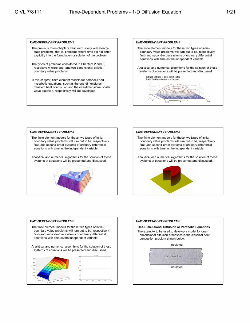
One-Dimensional Diffusion or Parabolic Equations
The example to be used to develop a model for one-dimensional diffusion processes is the classical heat conduction problem shown below:
Insulated
Insulated
CIVL 7/8111 Time-Dependent Problems - 1-D Diffusion Equation 1/21

TIME-DEPENDENT PROBLEMS
One-Dimensional Diffusion or Parabolic Equations
We will assume that energy in the form of heat flows only in the x-direction, that is, that there is no flux perpendicular to the x-axis.
The basic physical principle for this type of problem is balance of energy.
A differential element of length dx is isolated and an energy balance performed as:
ukA
x
u u
kA kA xx x x
energy in - energy out + internal energy generated =time rate of change of energy within the element
TIME-DEPENDENT PROBLEMS
One-Dimensional Diffusion or Parabolic Equations
The coefficients in the energy balance are:
k is the thermal conductivity,
is the mass density,
cp is the specific heat capacity, and
= k/(cp) is the thermal diffusivity
ukA
x
u u
kA kA xx x x
energy in - energy out + internal energy generated =time rate of change of energy within the element
TIME-DEPENDENT PROBLEMS
One-Dimensional Diffusion or Parabolic Equations
With the energy terms as indicated below, the balance of energy statement becomes:
ukA
x
u u
kA kA xx x x
energy in - energy out + internal energy generated =time rate of change of energy within the element
p
u u u ukA kA kA x qA x c A x
x x x x t
TIME-DEPENDENT PROBLEMS
One-Dimensional Diffusion or Parabolic Equations
In the limit as ∆x → 0:
ukA
x
u u
kA kA xx x x
energy in - energy out + internal energy generated =time rate of change of energy within the element
p
u ukA qA c A
x x t
TIME-DEPENDENT PROBLEMS
One-Dimensional Diffusion or Parabolic Equations
In the limit as ∆x → 0:
p
u ukA qA c A
x x t
This a second-order, linear partial differential equation. The auxiliary conditions consist of two boundary conditions and one initial condition.
An appropriate boundary condition prescribes either:
1. The dependent variable u
2. The flux:
3. a linear combination of the flux and the dependent variable:
ukA
x
u
kA hux
TIME-DEPENDENT PROBLEMS
One-Dimensional Diffusion or Parabolic Equations
This third type of boundary condition is called a convective boundary condition
It is a local energy balance between the convection externally and the conduction internally.
At the left boundary x = a, for instance, the external convective and internal conductive terms appear as:
( ) ( , )L Lh u t u a t ( , )u a tkA
x
CIVL 7/8111 Time-Dependent Problems - 1-D Diffusion Equation 2/21

TIME-DEPENDENT PROBLEMS
One-Dimensional Diffusion or Parabolic Equations
The local energy balance produces:
( , )( , ) ( )L L L
u a tkA h u a t h u t
x
A similar energy balance at the right end x = b yields:
( , )( , ) ( )R R R
u b tkA h u b t h u t
x
For a time-dependent diffusion problem it is also necessary to specify an initial value for the dependent variable of the form:
0( , 0) ( )u x u x
TIME-DEPENDENT PROBLEMS
One-Dimensional Diffusion or Parabolic Equations
The complete statement of the initial-boundary value problem consists of the differential equation, two boundary conditions, and an initial condition:
, 0p
u ukA qA c A a x b t
x x t
( , )( , ) ( ) 0L L L
u a tkA h u a t h u t t
x
( , )( , ) ( ) 0R R R
u b tkA h u b t h u t t
x
0( ,0) ( )u x u x a x b
TIME-DEPENDENT PROBLEMS
One-Dimensional Diffusion or Parabolic Equations
These equations represent a well-posed problem in partial differential equations.
, 0p
u ukA qA c A a x b t
x x t
( , )( , ) ( ) 0L L L
u a tkA h u a t h u t t
x
( , )( , ) ( ) 0R R R
u b tkA h u b t h u t t
x
0( ,0) ( )u x u x a x b
TIME-DEPENDENT PROBLEMS
One-Dimensional Diffusion or Parabolic Equations
When there is no convection at a boundary the other two types of boundary conditions appropriate at x = a are:
0( , 0) ( )u x u x
1. Where the temperature is specified:
( , )( )
u a tkA Q t
x
2. Where the energy flux is prescribed. The general development of the finite element model will assume type 3 conditions at both boundaries.
TIME-DEPENDENT PROBLEMS
One-Dimensional Diffusion or Parabolic Equations
The Galerkin Finite Element Method
Consider the one-dimensional diffusion problem developed in this section.
Discretization. The first step in developing a finite element model is discretization. Nodes for the spatial domain a ≤ x ≤ b are chosen as indicated below, with a = x1
and b = xN+1.
1x a 2x 4x · · ·Nx 1Nx b
u
x
nodes
3x
elements
TIME-DEPENDENT PROBLEMS
One-Dimensional Diffusion or Parabolic Equations
The Galerkin Finite Element Method
As was the case for steady-state problems considered in Chapter 2, the nodes are usually selected at equally spaced intervals, keeping in mind that it may be desirable in some problems to concentrate the nodes in regions of high gradients.
1x a 2x 4x · · ·Nx 1Nx b
u
x
nodes
3x
elements
CIVL 7/8111 Time-Dependent Problems - 1-D Diffusion Equation 3/21

TIME-DEPENDENT PROBLEMS
One-Dimensional Diffusion or Parabolic Equations
The Galerkin Finite Element Method
Interpolation. The interpolation functions are selected in exactly the same fashion as for the time-independent problem except that the nodal values are now taken to be functions of time rather than constants:
1
1
( , ) ( ) ( )N
i iu x t u t n x
The ni(x) are nodally based interpolation functions and can be linear, quadratic, or as otherwise desired.
TIME-DEPENDENT PROBLEMS
One-Dimensional Diffusion or Parabolic Equations
The Galerkin Finite Element Method
Interpolation. The interpolation functions are selected in exactly the same fashion as for the time-independent problem except that the nodal values are now taken to be functions of time rather than constants:
1
1
( , ) ( ) ( )N
i iu x t u t n x
The representation above is referred to as semidiscretization in that the spatial variable x is discretized whereas the temporal variable t is not.
TIME-DEPENDENT PROBLEMS
One-Dimensional Diffusion or Parabolic Equations
The Galerkin Finite Element Method
Interpolation. The interpolation functions are selected in exactly the same fashion as for the time-independent problem except that the nodal values are now taken to be functions of time rather than constants:
1
1
( , ) ( ) ( )N
i iu x t u t n x
A finite difference model of a time-dependent partial differential equation typically involves discretization of both the spatial and temporal variables.
TIME-DEPENDENT PROBLEMS
One-Dimensional Diffusion or Parabolic Equations
The Galerkin Finite Element Method
Elemental formulation. The elemental formulation for the diffusion problem is based on a corresponding weak statement.
The weak form is developed by multiplying the differential equation by a test function v(x) satisfying any homogeneous essential boundary conditions, and integrating over the spatial region according to:
0b
p
a
u uv kA qA c A dx
x x t
TIME-DEPENDENT PROBLEMS
One-Dimensional Diffusion or Parabolic Equations
The Galerkin Finite Element Method
Integrating by parts and eliminating the derivative terms from the boundary conditions yields:
( ) ( , ) ( ) ( , )
( ) ( ) ( ) ( )
b
pa
L R
b
L L R Ra
u uv kA c Av dx
x t
h v a u a t h v b u b t
vAq dx h v a u t h v b u t
Elemental formulation. The elemental formulation for the diffusion problem is based on a corresponding weak statement.
TIME-DEPENDENT PROBLEMS
One-Dimensional Diffusion or Parabolic Equations
The Galerkin Finite Element Method
This is the required weak statement for the class of one-dimensional diffusion problems.
( ) ( , ) ( ) ( , )
( ) ( ) ( ) ( )
b
pa
L R
b
L L R Ra
u uv kA c Av dx
x t
h v a u a t h v b u b t
vAq dx h v a u t h v b u t
Elemental formulation. The elemental formulation for the diffusion problem is based on a corresponding weak statement.
CIVL 7/8111 Time-Dependent Problems - 1-D Diffusion Equation 4/21

TIME-DEPENDENT PROBLEMS
One-Dimensional Diffusion or Parabolic Equations
The Galerkin Finite Element Method
Elemental formulation. The finite element model is obtained by substituting the approximate solution and v = nk, k = 1, 2, ..., N + 1, successively, into the above expression to obtain:
1
1
bN
k i i k p ia
n kAn u n c An u dx
1 1( ) ( )b
k L k L R kN Ra
n Aq dx h u t h u t
1 1 1 1( ) ( )L k R kN Nh u t h u t
TIME-DEPENDENT PROBLEMS
One-Dimensional Diffusion or Parabolic Equations
The Galerkin Finite Element Method
Elemental formulation. Which can be written as:
1
1
( ) ( ) ( ) 1,2,..., 1N
ki i ki i kA u t B u t q t k N
1 1
b
ki k i L k ik R kN ik
a
A n kAn dx h h
b
ki k p i
a
B n c An dx
1 1( ) ( )b
k k L k L R kN R
a
q n Aq dx h u t h u t
TIME-DEPENDENT PROBLEMS
One-Dimensional Diffusion or Parabolic Equations
The Galerkin Finite Element Method
Elemental formulation. In matrix notation, the above expression can be written as:
Au Bu q
e e e
G G GA k +BT B = m q = q +bt
T Tj j
i i
x x
p
x x
kA dx c A dx e ek N N m N N
j
i
x
x
qA dx eq N
TIME-DEPENDENT PROBLEMS
One-Dimensional Diffusion or Parabolic Equations
The Galerkin Finite Element Method
Elemental formulation. In matrix notation, the above expression can be written as:
e e e
G G GA k +BT B = m q = q +bt
T
0
( ) 0 0 .... 0 ( )0
0
L
L L R R
R
h
h u t h u t
h
BT bt
Au Bu q
TIME-DEPENDENT PROBLEMS
One-Dimensional Diffusion or Parabolic Equations
The Galerkin Finite Element Method
Elemental formulation. The original initial-boundary value problem has been converted into the initial value problem:
0with (0) Au Bu q u u
The initial vector u0 is usually taken to be a vector consisting of the values of u0(x) at the nodes:
T
0 0 0 2 0 3 0 0(0) ( ) ( ) ( ) ... ( ) ( )Nu a u x u x u x u b u u
Note that the assembly process has taken place implicitly during the process of carrying out the details of obtaining the governing equations using the Galerkin method.
TIME-DEPENDENT PROBLEMS
One-Dimensional Diffusion or Parabolic Equations
The Galerkin Finite Element Method
Elemental formulation. The original initial-boundary value problem has been converted into the initial value problem:
0with (0) Au Bu q u u
It is instructive to note that when time is not involved, the above equations are exactly what would result from the finite element model developed in Chapter 2 for the corresponding boundary value problem.
CIVL 7/8111 Time-Dependent Problems - 1-D Diffusion Equation 5/21

TIME-DEPENDENT PROBLEMS
One-Dimensional Diffusion or Parabolic Equations
The Galerkin Finite Element Method
Elemental formulation. The original initial-boundary value problem has been converted into the initial value problem:
0with (0) Au Bu q u u
Enforcement of constraints is necessary if either of the boundary conditions is essential, that is, if the dependent variable is prescribed at either boundary point.
The system equations must be altered to reflect these constraints.
TIME-DEPENDENT PROBLEMS
One-Dimensional Diffusion or Parabolic Equations
The Galerkin Finite Element Method
Elemental formulation. Consider for example the case where the boundary condition at x = a is u(a, t) = ua(t).
The hL terms in both BT and bt would be taken as zero and the first equation would be replaced by the constraint resulting in:
1
21 1 22 2 23 3 21 1 22 2 23 3 2
31 1 32 2 33 3 31 1 32 2 33 3 3
( )
( )
( )
au u t
a u a u a u b u b u b u q t
a u a u a u b u b u b u q t
1
22 2 23 3 22 2 23 3 2 21 1 21 1
22 2 23 3 22 2 23 3 3 31 1 31 1
( )
( )
( )
au u t
a u a u b u b u q t a u b u
a u a u b u b u q t a u b u
TIME-DEPENDENT PROBLEMS
One-Dimensional Diffusion or Parabolic Equations
The Galerkin Finite Element Method
Elemental formulation. Consider for example the case where the boundary condition at x = a is u(a, t) = ua(t).
The u1 and ů1 terms in the remaining equations are transferred to the right-hand side to yield
TIME-DEPENDENT PROBLEMS
One-Dimensional Diffusion or Parabolic Equations
The Galerkin Finite Element Method
Elemental formulation. For a linearly interpolated model the half bandwidth is two and only the terms involving u1
and ů1 in the second equation need to be transferred to the right-hand side.
For a quadratically interpolated model the half bandwidth is three and terms from the first two equations need to be transferred.
If the constraint is at the right end, the N th, (N - 1)st, . . . equations would be similarly altered.
TIME-DEPENDENT PROBLEMS
One-Dimensional Diffusion or Parabolic Equations
The Galerkin Finite Element Method
Elemental formulation. For a linearly interpolated model the half bandwidth is two and only the terms involving u1
and ů1 in the second equation need to be transferred to the right-hand side.
The constrained set of equations may be written as:
Mu Ku f 0(0) u u
TIME-DEPENDENT PROBLEMS
One-Dimensional Diffusion or Parabolic Equations
Example of One-Dimensional Diffusion
As a typical example consider the specific heat conduction problem:
0 , 0p
u ukA c A x L t
x x t
0(0, ) and ( , ) 0 0u t u u L t t
( ,0) 0 0u x x L
CIVL 7/8111 Time-Dependent Problems - 1-D Diffusion Equation 6/21

TIME-DEPENDENT PROBLEMS
One-Dimensional Diffusion or Parabolic Equations
Example of One-Dimensional Diffusion
This corresponds to the idealized situation of a region initially at zero temperature and whose left end x = 0 is instantaneously forced to assume the value u0 for all time greater than zero.
With A = constant and = k/cp the initial boundary value problem can be written as:
2
20 , 0
u ux L t
tx
0(0, ) and ( , ) 0 0u t u u L t t
( ,0) 0 0u x x L
TIME-DEPENDENT PROBLEMS
One-Dimensional Diffusion or Parabolic Equations
Example of One-Dimensional Diffusion
Discretization. For purposes of illustration, a four-element model will be investigated.
1 0x 2x 4x 5x L
u
x
3x
Interpolation. Linear interpolation will be used for the four elements.
TIME-DEPENDENT PROBLEMS
One-Dimensional Diffusion or Parabolic Equations
Example of One-Dimensional Diffusion
Elemental Formulation.
1
1
ii
i i
x xN
x x
11
ii
i i
x xN
x x
ix 1ix
1
iN
1
1iN
ix 1ix
TIME-DEPENDENT PROBLEMS
One-Dimensional Diffusion or Parabolic Equations
Example of One-Dimensional Diffusion
Elemental Formulation. The elemental matrices are:
1
1i
i i
Nx x
1
1
1i
i i
Nx x
11 1iN
ix 1ix
1iN
ix 1ix
1
TIME-DEPENDENT PROBLEMS
One-Dimensional Diffusion or Parabolic Equations
Example of One-Dimensional Diffusion
Elemental Formulation. The elemental matrices are:
1
Ti
i
x
x
dxek N N
1
1
1 1
1
1
1 1
1
i
i
xi i
i i i ix
i i
x xdx
x x x x
x x
TIME-DEPENDENT PROBLEMS
One-Dimensional Diffusion or Parabolic Equations
Example of One-Dimensional Diffusion
Elemental Formulation. The elemental matrices are:
1
Ti
i
x
x
dxek N N
1
2
1
111 1
1
i
i
x
xi i
dxx x
1
2
1 1
1 1
i
i
x
e x
dxl
1 1
1 1el
1 14
1 1L
CIVL 7/8111 Time-Dependent Problems - 1-D Diffusion Equation 7/21

TIME-DEPENDENT PROBLEMS
One-Dimensional Diffusion or Parabolic Equations
Example of One-Dimensional Diffusion
Elemental Formulation. The elemental matrices are:
1i
i
x
x
dxTem NN
1i
i
x
x
dxTe1m NN
/4 4
4 44
0
11
L xL x x
L LxL
dx
2 1
1 224
L
1
1
1 1
1 1
1
i
i
ix
i i i i
i i i i ix
i i
x x
x x x x x xdx
x x x x x x
x x
At xi = 0 and xi+1 = L/4, then
/4
0
L
dxTe1m NN
TIME-DEPENDENT PROBLEMS
One-Dimensional Diffusion or Parabolic Equations
Example of One-Dimensional Diffusion
Elemental Formulation. The elemental matrices are:
1
T 1 14
1 1
i
i
x
x
dxLek N N
1
T 2 1
1 224
i
i
x
x
Ldxem NN
1
0i
i
x
x
q dxeq N
TIME-DEPENDENT PROBLEMS
One-Dimensional Diffusion or Parabolic Equations
Example of One-Dimensional Diffusion
Assembly. With both the boundary conditions essential, BT=0 and bt=0. It follows that the assembled equations are:
0 Au Bu
1 1 0 0 0
1 2 1 0 04
0 1 2 1 0
0 0 1 2 1
0 0 0 1 1
Ge
kL
A
T
1 2 3 4 5u u u u uu
2 1 0 0 0
1 4 1 0 0
0 1 4 1 024
0 0 1 4 1
0 0 0 1 2
Ge
Lm
B
The initial condition is homogeneous so that: (0) 0u
TIME-DEPENDENT PROBLEMS
One-Dimensional Diffusion or Parabolic Equations
Example of One-Dimensional Diffusion
Constraints. The constraints follow from the boundary conditions as:
1 0 5and 0u u u
The constrained equations become:
02 1 0 4 1 0
1 2 1 1 4 1 0
0 1 2 0 1 4 0
u
u u 2
96
L
Subject to the initial condition: 0(0) uu
TIME-DEPENDENT PROBLEMS
One-Dimensional Diffusion or Parabolic Equations
Example of One-Dimensional Diffusion
These approximate equations must now be integrated for an estimate of the time-dependent solution.
Appropriate analytical and numerical methods of integration are presented and discussed in the following sections.
02 1 0 4 1 0
1 2 1 1 4 1 0
0 1 2 0 1 4 0
u
u u 2
96
L
TIME-DEPENDENT PROBLEMS
One-Dimensional Diffusion or Parabolic Equations
Example of One-Dimensional Diffusion
The elemental mass matrices me are referred to as consistent mass matrices in that they are determined on the basis of the same interpolation functions as were used for the corresponding stiffnesses ke.
1
Ti
i
x
p
x
c A dxem N N
1
1
1 1
1 1
1
i
i
ix
i i i ip
i i i i ix
i i
x x
x x x x x xc A dx
x x x x x x
x x
CIVL 7/8111 Time-Dependent Problems - 1-D Diffusion Equation 8/21

TIME-DEPENDENT PROBLEMS
One-Dimensional Diffusion or Parabolic Equations
Example of One-Dimensional Diffusion
The elemental mass matrices me are referred to as consistent mass matrices in that they are determined on the basis of the same interpolation functions as were used for the corresponding stiffnesses ke.
1
Ti
i
x
p
x
c A dxem N N
1
0
11 1
1 p ec A l dx
2 1
1 26p ec Al
10
21
02
p ec Allem
TIME-DEPENDENT PROBLEMS
One-Dimensional Diffusion or Parabolic Equations
Example of One-Dimensional Diffusion
Another approach to generating mass matrices is referred to as lumping with the results referred to as lumped mass matrices. The idea is simply that the total mass associated with the consistent mass matrix:
The term cpAle, is split between the two nodes to form a diagonal mass matrix called a lumped mass matrix mle:
3 0
0 36p ec Al
TIME-DEPENDENT PROBLEMS
One-Dimensional Diffusion or Parabolic Equations
Example of One-Dimensional Diffusion
This lumped mass matrix has advantages in certain of the time integration algorithms to be discussed in later sections.
Also, it has the interesting property that the resulting eigenvalues are generally smaller than the exact values.
Eigenvalues are generally overestimated when using the consistent mass matrices.
TIME-DEPENDENT PROBLEMS
One-Dimensional Diffusion or Parabolic Equations
Example of One-Dimensional Diffusion
This suggests that a third possibility for treating the mass is to consider a weighted average of the consistent mass matrix mce and lumped mass matrix mle according to:
1 w ce lem m m
If = ½ then:
2 1 3 01
1 2 0 32 6p ec Al
wm
5 1
1 512el
TIME-DEPENDENT PROBLEMS
One-Dimensional Diffusion or Parabolic Equations
Example of One-Dimensional Diffusion
This is one of the so-called higher-order accurate mass matrices.
Its use results in improved estimates for the eigenvalues as compared with estimates using either of the consistent or lumped mass matrix formulations.
The corresponding result for the quadratically interpolated element turns out to be:
9 2 1
2 36 260
1 2 9
el
wm
TIME-DEPENDENT PROBLEMS
One-Dimensional Diffusion or Parabolic Equations
Analytical Integration Techniques
An analytical approach to the integration of the set of equations decomposes the solution of:
into + h pKu Mu f u u u
where uh is the homogeneous solution satisfying:
0 h hKu Mu
and up is any particular solution satisfying:
p pKu Mu f
CIVL 7/8111 Time-Dependent Problems - 1-D Diffusion Equation 9/21

TIME-DEPENDENT PROBLEMS
One-Dimensional Diffusion or Parabolic Equations
Analytical Integration Techniques
Homogenous Solution. For the case where K and M are matrices of constants:
is a set of linear constant-coefficient, ordinary differential equations.
When K and M are not constant matrices, it is necessary to use techniques such as discussed in the next section.
( ) 0t h hKu Mu =
TIME-DEPENDENT PROBLEMS
One-Dimensional Diffusion or Parabolic Equations
Analytical Integration Techniques
Homogenous Solution. The standard approach to the solution of such a constant coefficient system is to assume:
where v is a vector of constants.
The negative sign in the exponential function is a matter of anticipating the decaying character of the solution of diffusion problems.
( ) tt e hu v
TIME-DEPENDENT PROBLEMS
One-Dimensional Diffusion or Parabolic Equations
Analytical Integration Techniques
Homogenous Solution. Substitute:
Thus the homogeneous solutions are obtained by solving the generalized linear algebraic eigenvalue problem.
Nontrivial solutions of this expression require:
( ) tt e hu v
0te K M v 0 K M v
det 0 K M
TIME-DEPENDENT PROBLEMS
One-Dimensional Diffusion or Parabolic Equations
Analytical Integration Techniques
Homogenous Solution. The eigenvalues are obtained 1, 2, … and the corresponding eigenvectors v1, v2, … are then determined by back-substituting the eigenvalues one at a time.
The analytical approach is quite valuable from the stand-point that the results can be immediately interpreted in terms of the decay rates [exp(-it) as determined by the eigenvalues] that will be present in the solution regardless of whether an analytical or a numerical approach is being used.
These eigenvalues are an important part of the discussions of convergence and stability covered in later sections.
TIME-DEPENDENT PROBLEMS
One-Dimensional Diffusion or Parabolic Equations
Analytical Integration Techniques
Homogenous Solution. For the particular example, the equations can be written as:
2 1 0 4 1 0
1 2 1 1 4 1 0
0 1 2 0 1 42
96
L
det 0 K M
2
96
L
2 1 0 4 1 0
1 2 1 1 4 1 0
0 1 2 0 1 4
TIME-DEPENDENT PROBLEMS
One-Dimensional Diffusion or Parabolic Equations
Analytical Integration Techniques
Homogenous Solution. For the particular example, the equations can be written as:
2 4 1 0
det 1 2 4 1 0
0 1 2 4
K M
3 256 76 32 4 0
1 2 30.1082 0.5000 1.3204
CIVL 7/8111 Time-Dependent Problems - 1-D Diffusion Equation 10/21

TIME-DEPENDENT PROBLEMS
One-Dimensional Diffusion or Parabolic Equations
Analytical Integration Techniques
Homogenous Solution. The roots of the corresponding characteristic equation:
1 2 30.1082 0.5000 1.3204
1 2 32 2 2
10.387 48.000 126.76L L L
Which compares to the exact eigenvalues of:
2 2 2
1 2 32 2 2
4 9
L L L
TIME-DEPENDENT PROBLEMS
One-Dimensional Diffusion or Parabolic Equations
Analytical Integration Techniques
Homogenous Solution. The roots of the corresponding characteristic equation:
1 2 30.1082 0.5000 1.3204
1 2 32 2 2
10.387 48.000 126.76L L L
Which compares to the exact eigenvalues of:
1 2 32 2 2
9.8696 39.478 88.826
L L L
TIME-DEPENDENT PROBLEMS
One-Dimensional Diffusion or Parabolic Equations
Analytical Integration Techniques
Homogenous Solution. It can easily be seen that, roughly, the solutions will decay to steady state too rapidly in view of the fact that the ’s predicted by the finite element solution are larger than the corresponding exact values.
1 2 32 2 2
10.387 48.000 126.76L L L
Which compares to the exact eigenvalues of:
1 2 32 2 2
9.8696 39.478 88.826
L L L
TIME-DEPENDENT PROBLEMS
One-Dimensional Diffusion or Parabolic Equations
Analytical Integration Techniques
Homogenous Solution. The corresponding eigenvectors obtained by back-substitution:
And the homogeneous solution can then be written as:
1 2 3
1 11
2 0 2
1 1 1
v v v
31 21 1 2 2 3 3( ) tt tt c v e c v e c v e hu
TIME-DEPENDENT PROBLEMS
One-Dimensional Diffusion or Parabolic Equations
Analytical Integration Techniques
Particular Solution. For the particular solution, consider:
By inspection (Method of Intelligent Guessing!) it can be see that by taking up=d, a constant, there results:
01
2 1 0 4 1 0
1 2 1 1 4 1 0
0 1 2 0 1 4 0
u
p pu u
2
96L
T0 3 2 14
ud
TIME-DEPENDENT PROBLEMS
One-Dimensional Diffusion or Parabolic Equations
Analytical Integration Techniques
The general solution can then be written as:
Satisfying the initial conditions u(0) = 0 leads to the set of linear algebraic equations:
31 21 1 2 2 3 3
tt tc v e c v e c v e pu u
0
1
02
30
3
41 1 12
2 0 24
1 1 1
4
u
cu
c
cu
1 2 3v v v
CIVL 7/8111 Time-Dependent Problems - 1-D Diffusion Equation 11/21

TIME-DEPENDENT PROBLEMS
One-Dimensional Diffusion or Parabolic Equations
Analytical Integration Techniques
Solving the set of linear algebraic equations yields:
1 0 2 0 3 00.4268 0.2500 0.0732c u c u c u
The solution can finally be expressed as:
31 21 1 2 2 3 3
tt tc v e c v e c v e pu u
1 2 3
1 11
2 0 2
1 1 1
v v v
TIME-DEPENDENT PROBLEMS
One-Dimensional Diffusion or Parabolic Equations
Analytical Integration Techniques
Solving the set of linear algebraic equations yields:
1 0 2 0 3 00.4268 0.2500 0.0732c u c u c u
31 22
0
( )0.7500 0.4268 0.2500 0.0732 tt tu t
e e eu
313
0
( )0.5000 0.6036 0.1036 ttu t
e eu
31 24
0
( )0.2500 0.4268 0.2500 0.0732 tt tu t
e e eu
The solution can finally be expressed as:
pu
TIME-DEPENDENT PROBLEMS
One-Dimensional Diffusion or Parabolic Equations
Analytical Integration Techniques
Note that as:
The solution can finally be expressed as:
This is the correct steady state solution.
2 0 3 0 4 0, ( ) 0.7500 , ( ) 0.5000 , ( ) 0.2500 ,t u t u u t u u t u
31 22
0
( )0.7500 0.4268 0.2500 0.0732 tt tu t
e e eu
313
0
( )0.5000 0.6036 0.1036 ttu t
e eu
31 24
0
( )0.2500 0.4268 0.2500 0.0732 tt tu t
e e eu
TIME-DEPENDENT PROBLEMS
One-Dimensional Diffusion or Parabolic Equations
Analytical Integration Techniques
As mentioned previously, the finite element model predicts that these steady-state values are reached too quickly.
For a specific case assume that the bar is 0.2 m in length and is composed of an aluminum alloy for which = 8.4 x 10⁻⁴ m2/s, from which /L2 = 0.021 s-1.
TIME-DEPENDENT PROBLEMS
One-Dimensional Diffusion or Parabolic Equations
Analytical Integration Techniques
Four-element analytical versus exact solution
t (sec) (u2/u0) (u2/u0)exact (u3/u0) (u3/u0)exact (u4/u0) (u4/u0)exact
1.0 0.3105 0.2225 0.0219 0.0147 -0.0070 0.0003
2.0 0.4404 0.3884 0.1103 0.0845 0.0070 0.0096
3.0 0.5106 0.4812 0.1863 0.1589 0.0403 0.0342
4.0 0.5672 0.5419 0.2478 0.2223 0.0761 0.0650
5.0 0.6050 0.5852 0.2972 0.2742 0.1082 0.0953
6.0 0.6341 0.6180 0.3369 0.3164 0.1353 0.1224
7.0 0.6571 0.6435 0.3689 0.3508 0.1575 0.1455
8.0 0.6754 0.6638 0.3946 0.3787 0.1755 0.1647
9.0 0.6900 0.6801 0.4152 0.4014 0.1901 0.1805
10.0 0.7018 0.6933 0.4319 0.4199 0.2018 0.1934
15.0 0.7338 0.7299 0.4771 0.4716 0.2338 0.2299
20.0 0.7446 0.7429 0.4923 0.4899 0.2446 0.2429
TIME-DEPENDENT PROBLEMS
One-Dimensional Diffusion or Parabolic Equations
Analytical Integration Techniques
,3
Lu t
As mentioned previously and as can easily be seen from these data, the finite element solution tends towards steady state too rapidly.
CIVL 7/8111 Time-Dependent Problems - 1-D Diffusion Equation 12/21

TIME-DEPENDENT PROBLEMS
One-Dimensional Diffusion or Parabolic Equations
Analytical Integration Techniques
,4
Lu t
The trend is of course helped by taking more elements, in which case the approximate eigenvalues arising from the finite element model approach the exact.
TIME-DEPENDENT PROBLEMS
One-Dimensional Diffusion or Parabolic Equations
Analytical Integration Techniques
,3
Lu t
With more elements the results are correspondingly closer to those given by the exact solution.
TIME-DEPENDENT PROBLEMS
One-Dimensional Diffusion or Parabolic Equations
Analytical Integration Techniques
With more elements the results are correspondingly closer to those given by the exact solution.
-0.1
0
0.1
0.2
0.3
0.4
0.5
0.6
0.7
0.8
0 2 4 6 8 10 12 14 16 18 20
Time (sec)
,4
Lu t
,2
Lu t
3,
4
Lu t
TIME-DEPENDENT PROBLEMS
One-Dimensional Diffusion or Parabolic Equations
Time Integration Techniques – First-Order Systems
In situations where M and/or K in:
0with (0) Mu Ku f u u
are functions of t or where f is such that a particular solution by analytic means is difficult or impossible, the analytical technique discussed may be practically impossible to carry through.
Depending on the particulars, numerical techniques are attractive or even necessary to carry out the integration.
TIME-DEPENDENT PROBLEMS
One-Dimensional Diffusion or Parabolic Equations
Time Integration Techniques – First-Order Systems
The Euler Method - Recall that for a first-order initial value problem of the form:
it is possible to develop numerical integration schemes for the approximate integration of the initial value problem.
The problem is to determine a function y(x) passing through the initial point (x0, y0) and satisfying the differential equation y' = f
0 0( , ) with ( )y f x y y x y
TIME-DEPENDENT PROBLEMS
One-Dimensional Diffusion or Parabolic Equations
Time Integration Techniques – First-Order Systems
The Euler Method - Recall that for a first-order initial value problem of the form:
0 0( , ) with ( )y f x y y x y
CIVL 7/8111 Time-Dependent Problems - 1-D Diffusion Equation 13/21

TIME-DEPENDENT PROBLEMS
One-Dimensional Diffusion or Parabolic Equations
Time Integration Techniques – First-Order Systems
In the Euler Method, the derivative y′ is represented as a forward difference according to:
1
1
n n
n n
y yy
x x
TIME-DEPENDENT PROBLEMS
One-Dimensional Diffusion or Parabolic Equations
Time Integration Techniques – First-Order Systems
Giving a linear approximation to the derivative at xn with h = xn+1 – xn. The differential equation at xn is:
1 ,n nn n
y yy f x y
h
TIME-DEPENDENT PROBLEMS
One-Dimensional Diffusion or Parabolic Equations
Time Integration Techniques – First-Order Systems
Solving for yn+1 results in: 1 ,n n n ny y hf x y
TIME-DEPENDENT PROBLEMS
One-Dimensional Diffusion or Parabolic Equations
Time Integration Techniques – First-Order Systems
Starting with y(x0) = y0, this algorithm can be used to step ahead in the independent variable x to determine an approximate solution.
Note that the Euler Method can also be viewed in the following manner.
Integrate the differential equation between the limits of xn
and xn+1 to obtain:
1 1
1 ,n n
n n
x x
n n
x x
y dx y y f x y dx
TIME-DEPENDENT PROBLEMS
One-Dimensional Diffusion or Parabolic Equations
Time Integration Techniques – First-Order Systems
Approximate the remaining integral by to obtain:
1 ,n n n ny y hf x y
The integral has been approximated by evaluating f at the left end of the interval over which the integral is evaluated and multiplying by the interval h.
This is again clearly the Euler algorithm.
TIME-DEPENDENT PROBLEMS
One-Dimensional Diffusion or Parabolic Equations
Time Integration Techniques – First-Order Systems
The analogue of the Euler Method for the system of equations:
is obtained by again representing the derivative term at a particular value of the time tn as a forward difference according to:
0with (0) Mu Ku f u u
1n nn h
u uu
CIVL 7/8111 Time-Dependent Problems - 1-D Diffusion Equation 14/21

TIME-DEPENDENT PROBLEMS
One-Dimensional Diffusion or Parabolic Equations
Time Integration Techniques – First-Order Systems
And evaluating the differential equation at t = tn to obtain:
From which the Euler algorithm is obtained:
n n n Mu Ku f
1 0(0)n n nh h u Mu M K u f u
1n nnh
u uM Ku
TIME-DEPENDENT PROBLEMS
One-Dimensional Diffusion or Parabolic Equations
Time Integration Techniques – First-Order Systems
And evaluating the differential equation at t = tn to obtain:
The utility and effectiveness of the algorithm is affected by its stability, that is, by whether for large time the solution predicted by the algorithm remains finite, independent of the step size h.
1 0 0 1h h Mu M K u f u
2 1 1 2h h Mu M K u f u
3 2 2 3h h Mu M K u f u
TIME-DEPENDENT PROBLEMS
One-Dimensional Diffusion or Parabolic Equations
Time Integration Techniques – First-Order Systems
And evaluating the differential equation at t = tn to obtain:
The Euler algorithm is conditionally stable: there is a critical step size hcr such that when h > hcr the solution oscillates with ever increasing amplitude, obviously negating the results of the algorithm.
1 0 0 1h h Mu M K u f u
2 1 1 2h h Mu M K u f u
3 2 2 3h h Mu M K u f u
TIME-DEPENDENT PROBLEMS
One-Dimensional Diffusion or Parabolic Equations
Time Integration Techniques – First-Order Systems
The use of the Euler algorithm results in a local discret-ization error e, which depends upon the step size h according to:
indicating that when the time step h is halved the local discretization error is reduced approximately by 1/4.
The accumulated discretization error E is given by:
2e O h
E O h
TIME-DEPENDENT PROBLEMS
One-Dimensional Diffusion or Parabolic Equations
Time Integration Techniques – First-Order Systems
The accumulated discretization error is approximately halved by halving the integration time step.
One might assume on the basis of these results that by decreasing the step size sufficiently the error could be decreased indefinitely.
This is not the case in that the roundoff error begins to dominate the process for h too small.
TIME-DEPENDENT PROBLEMS
One-Dimensional Diffusion or Parabolic Equations
Time Integration Techniques – First-Order Systems
Example 1 – Consider the application of the Euler algorithm to the set of equations previously developed for the four-element problem:
4 1 0 2 1 0 1
1 4 1 1 2 1 0
0 1 4 0 1 2 0
w w
2
96
L Ku Mu f
0u
uw
1n n nh hMw M K w f
CIVL 7/8111 Time-Dependent Problems - 1-D Diffusion Equation 15/21

TIME-DEPENDENT PROBLEMS
One-Dimensional Diffusion or Parabolic Equations
Time Integration Techniques – First-Order Systems
These equations become:
1
4 1 0 4 1 0 2 1 0 1
1 4 1 1 4 1 1 2 1 0
0 1 4 0 1 4 0 1 2 0n nh h
w w
For this set of equation the inverse of M can be determined, so that the equations may be written as:
1
1 0 0 34 24 6 15
0 1 0 24 40 24 456 56
0 0 1 6 24 34 1n n
h h
w w
TIME-DEPENDENT PROBLEMS
One-Dimensional Diffusion or Parabolic Equations
Time Integration Techniques – First-Order Systems
With /L2 = 0.021 s-1 and h = 0.1 s the equations become:
1
0.8776 0.0864 0.0216 0.0540
0.0864 0.8560 0.0864 0.0144
0.0216 0.0864 0.8776 0.0036n n
w w
1n n w Sw b
TIME-DEPENDENT PROBLEMS
One-Dimensional Diffusion or Parabolic Equations
Time Integration Techniques – First-Order Systems
With w(0) = 0, successive iterations of the equations give:
The algorithm is repeatedly applied until the range of times of interest is covered.
T
1 0.0540 0.0144 0.0036 w bT
2 1 0.1001 0.0217 0.0043 w Sw bT
3 2 0.1398 -0.0240 0.0034 w Sw b
TIME-DEPENDENT PROBLEMS
One-Dimensional Diffusion or Parabolic Equations
Time Integration Techniques – First-Order Systems
The algorithm in the example is used with several values of the step size h = t.
Approximate solution w3(t) for different h using the Euler algorithm
t (sec) h = 0.083 h = 0.167 h = 0.333 h = 1.0 uexact
1 0.0208 0.0198 0.0189 -0.1440 0.01472 0.1116 0.1131 0.1163 0.4170 0.08453 0.1881 0.1901 0.1940 -0.2683 0.15894 0.2497 0.2518 0.2560 1.0643 0.22235 0.2991 0.3013 0.3055 0.9891 0.27426 0.3388 0.3409 0.3449 2.5436 0.31647 0.3706 0.3726 0.3763 -3.2333 0.35088 0.3962 0.3980 0.4014 6.4408 0.37879 0.4167 0.4183 0.4214 -9.5789 0.4014
10 0.4331 0.4346 0.4373 17.0888 0.419920 0.4926 0.4929 0.4935 2674.49 0.4899
TIME-DEPENDENT PROBLEMS
One-Dimensional Diffusion or Parabolic Equations
Time Integration Techniques – First-Order Systems
These results show clearly several aspects of the numerical solution:
1. The approximate solution tends toward steady state more rapidly than the exact solution. This property is primarily attributable to the eigenvalues of M - K being larger than the exact eigenvalues.
2. There is clearly a step size h above which the approximate solution is unstable as indicated by the h= 1.0 results.
3. When the step size is not exceeded, the approximate solution approaches the correct steady-state values for large t.
TIME-DEPENDENT PROBLEMS
One-Dimensional Diffusion or Parabolic Equations
Time Integration Techniques – First-Order Systems
These results show clearly several aspects of the numerical solution:
4. If lumping is used, the assembled mass matrix M is diagonal and easily inverted. The integration procedure is reduced at each step to a simple matrix multiplication and vector addition:
11n n nh u Su M f
where if M and K are constant matrices, S = I - hM-1Kcan be computed at the first time step and used thereafter for the subsequent applications of the basic algorithm.
CIVL 7/8111 Time-Dependent Problems - 1-D Diffusion Equation 16/21

TIME-DEPENDENT PROBLEMS
One-Dimensional Diffusion or Parabolic Equations
Time Integration Techniques – First-Order Systems
The Improved Euler or Crank-Nicolson Method - The improved Euler or Crank-Nicolson algorithm can be thought of is the following way.
The improved Euler algorithm is developed according to:
0 0( , ) with ( )y f x y y x y
1 1
1
, ,
2n n n n
n n
h f x y f x yy y
TIME-DEPENDENT PROBLEMS
One-Dimensional Diffusion or Parabolic Equations
Time Integration Techniques – First-Order Systems
That is, the integral:
has been evaluated by taking the average of f at the ends of the interval (xn, xn+1).
For the vector equation in question, the corresponding expression is:
1
,n
n
x
x
f x y dx
11 2
n nn n
h
u uu u
TIME-DEPENDENT PROBLEMS
One-Dimensional Diffusion or Parabolic Equations
Time Integration Techniques – First-Order Systems
This is equivalent to a central difference representation for the derivative ů. Multiplying through by M yields:
which, on using the differential equation Mů + Ku = f, can be written as:
11 2
n nn n
h
Mu MuMu Mu
1 1 1
n n n
n n n
Mu f KuMu f Ku
Mu f Ku
TIME-DEPENDENT PROBLEMS
One-Dimensional Diffusion or Parabolic Equations
Time Integration Techniques – First-Order Systems
This is equivalent to a central difference representation for the derivative ů. Multiplying through by M yields:
which, on using the differential equation Mů + Ku = f, can be written as:
11 2
n nn n
h
Mu MuMu Mu
112 2 2
n nn n
hh h
f fK KM u M u
TIME-DEPENDENT PROBLEMS
One-Dimensional Diffusion or Parabolic Equations
Time Integration Techniques – First-Order Systems
This is the improved Euler or Crank-Nicolson algorithm.
As opposed to the algorithm studied in the last section, this algorithm is unconditionally stable, that is, although the accuracy may suffer considerably and oscillations occur for a large step size h, the oscillations never become unbounded.
In addition to being unconditionally stable, the improved Euler or Crank-Nicolson algorithm is one order more accurate than the previously developed Euler algorithm in that the accumulated discretization error E is given approximately by E = O(h2).
TIME-DEPENDENT PROBLEMS
One-Dimensional Diffusion or Parabolic Equations
Time Integration Techniques – First-Order Systems
To implement the method, write the equations as:
1 1n n Au b
112 2 2
n nn n
hh h
f fK KA M b M u
This set of linear algebraic equations must be solved at each time step.
CIVL 7/8111 Time-Dependent Problems - 1-D Diffusion Equation 17/21

TIME-DEPENDENT PROBLEMS
One-Dimensional Diffusion or Parabolic Equations
Time Integration Techniques – First-Order Systems
Given u(0) = u0,
is to be solved for u1, after which:
1 1 0
0
2 2
h h h
f f KAu b M u
2 2 1
2
2 2
h h h h
f f KAu b M u
is to be solved for u2, and so forth.
TIME-DEPENDENT PROBLEMS
One-Dimensional Diffusion or Parabolic Equations
Time Integration Techniques – First-Order Systems
As long as h = constant, the same coefficient matrix M+hK/2is involved at each step and it is economical to use an equation solver that decomposes A at the first step according to A = LU.
This decomposition is then saved so that at each succeeding step, two triangular systems can be solved.
This is substantially more economical than to solve Ax = bat each step.
TIME-DEPENDENT PROBLEMS
One-Dimensional Diffusion or Parabolic Equations
Time Integration Techniques – First-Order Systems
In the event that M and K are functions of t, then M, K, M + hK/2, and M - hK/2 must potentially be recomputed at each step.
If the variation of these matrices with time is small, recalculation of the necessary matrices and decomposition of M + hK/2 can be done at suitable regular intervals rather than at each time step
TIME-DEPENDENT PROBLEMS
One-Dimensional Diffusion or Parabolic Equations
Time Integration Techniques – First-Order Systems
Example 2 - Consider the previous example with the following set of equations
4 1 0 2 1 0 1
1 4 1 1 2 1 0
0 1 4 0 1 2 0
w w
2
96
L Ku Mu f
0u
uw
TIME-DEPENDENT PROBLEMS
One-Dimensional Diffusion or Parabolic Equations
Time Integration Techniques – First-Order Systems
Generally,
2
4 1 0 2 1 048
1 4 1 1 2 12
0 1 4 0 1 2
h h
L
KM
Taking = 8.4 x 10⁻⁴ m2/s, L = 0.2 m, and h = 0.1s results in:
4.2016 0.8992 0.0000
0.8992 4.2016 0.89922
0.0000 0.8992 4.2016
h
KM
3.7984 1.1008 0.0000
1.1008 3.7984 1.10082
0.0000 1.1008 3.7984
h
KM
TIME-DEPENDENT PROBLEMS
One-Dimensional Diffusion or Parabolic Equations
Time Integration Techniques – First-Order Systems
The 3 x 3 matrix M + hK/2 can be inverted so that there results specifically:
1
0.8879 0.0754 0.0161 0.0504
0.0754 0.8718 0.0754 0.0113
0.0161 0.0754 0.8879 0.0024n n
w w
1 (0) 0n n w Sw b w
CIVL 7/8111 Time-Dependent Problems - 1-D Diffusion Equation 18/21

TIME-DEPENDENT PROBLEMS
One-Dimensional Diffusion or Parabolic Equations
Time Integration Techniques – First-Order Systems
The first couple of iterations yield:
T
2 1 0.1011 0.0169 0.0028 w Sw b
with iteration being continued until the time interval of interest is covered.
T
1 0.0540 0.0113 0.0024 w b
T
3 2 0.1424 0.0182 0.0020 w Sw b
TIME-DEPENDENT PROBLEMS
One-Dimensional Diffusion or Parabolic Equations
Time Integration Techniques – First-Order Systems
For this example, results are given for several values of h for u3(t) along with those as given by the exact solution.
Approximate solution u3(t) for different h using the improved Euler algorithm
t (sec) h = 0.083 h = 0.167 h = 0.333 h = 1.0 uexact
1 0.0219 0.0216 0.0207 0.0004 0.0147
2 0.1103 0.1103 0.1102 0.1126 0.08453 0.1863 0.1863 0.1864 0.1868 0.15894 0.2478 0.2478 0.2479 0.2487 0.22235 0.2972 0.2972 0.2973 0.2981 0.27426 0.3369 0.3370 0.3370 0.3378 0.31647 0.3689 0.3689 0.3690 0.3697 0.35088 0.3946 0.3946 0.3947 0.3953 0.37879 0.4153 0.4153 0.4153 0.4159 0.401410 0.4319 0.4319 0.4319 0.4324 0.419920 0.4923 0.4923 0.4923 0.4924 0.4899
TIME-DEPENDENT PROBLEMS
One-Dimensional Diffusion or Parabolic Equations
Time Integration Techniques – First-Order Systems
Comparing these results with the results presented using the Euler method; the following observations can be made:
1. The results using the improved Euler algorithm are more accurate than those from the Euler algorithm, with steady state not being approached as rapidly using the improved Euler algorithm.
2. For the values of h investigated, the improved Euler algorithm is stable.
3. Lumping does not result in any computational advantage for the improved Euler algorithm since the coefficient matrix is M + hK/2 rather than M as for the Euler algorithm.
TIME-DEPENDENT PROBLEMS
One-Dimensional Diffusion or Parabolic Equations
ANALYSIS OF ALGORITHMS
Both the Euler and improved Euler or Crank-Nicolson algorithms presented in the preceding sections can be considered as special cases of the so-called algorithm that assumes:
1 1 1n n n nh u u u u
that is, a weighted sum of the derivatives at the beginning and end of the interval (tn, tn+1) is used to evaluate the integral:
1n
n
t
n
t
dt
u
TIME-DEPENDENT PROBLEMS
One-Dimensional Diffusion or Parabolic Equations
ANALYSIS OF ALGORITHMS
Multiplying the algorithm by M and subsequently using the differential equation to eliminate the Mu terms yields:
It is easily seen that:
1 1(1 ) 1n n n nh h h M K u M K u f f
12
0 Euler method
Crank-Nicolson method
The value = 1 corresponds to what is referred to as the modified Euler method and corresponds to using a backward difference scheme obtained by evaluating the differential equation at tn+1 and taking:
11
n nn h
u uu
TIME-DEPENDENT PROBLEMS
One-Dimensional Diffusion or Parabolic Equations
ANALYSIS OF ALGORITHMS
Example - As a very simple demonstration, consider a two-element model for the previous problem.
with (0) 02
w w w
where w = u2lu0 and = 12/L2.
The eigenvalue is determined by taking w = c exp(-t) in the homogeneous equation leading to = = 12/L2.
The method yields:
1
1 (1 ) / 2
(1 )n
n
h w hw
h
CIVL 7/8111 Time-Dependent Problems - 1-D Diffusion Equation 19/21

TIME-DEPENDENT PROBLEMS
One-Dimensional Diffusion or Parabolic Equations
ANALYSIS OF ALGORITHMS
Example – The results from the Euler, the Crank-Nicolson, and the modified Euler algorithms, along with the analytical solution, for h = 0.1, 1.0, 2.0, and 2.2, respectively.
Comparison of numerical and analytical solutions for p = h = 0.1
Step # Euler C-N M-Euler Analytical
1 0.0500 0.0476 0.0455 0.0476
2 0.0950 0.0907 0.0868 0.0906
3 0.1355 0.1297 0.1243 0.1296
4 0.1720 0.1650 0.1585 0.1648
5 0.2048 0.1969 0.1895 0.1967
6 0.2343 0.2257 0.2178 0.2256
7 0.2609 0.2519 0.2434 0.2517
8 0.2848 0.2755 0.2667 0.2753
9 0.3063 0.2969 0.2880 0.2967
10 0.3257 0.3162 0.3072 0.3161
TIME-DEPENDENT PROBLEMS
One-Dimensional Diffusion or Parabolic Equations
ANALYSIS OF ALGORITHMS
Example – The results from the Euler, the Crank-Nicolson, and the modified Euler algorithms, along with the analytical solution, for h = 0.1, 1.0, 2.0, and 2.2, respectively.
Comparison of numerical and analytical solutions for p = h = 1.0
Step # Euler C-N M-Euler Analytical
1 0.5000 0.3333 0.2500 0.3161
2 0.5000 0.4444 0.3750 0.4323
3 0.5000 0.4815 0.4375 0.4751
4 0.5000 0.4938 0.4688 0.4908
5 0.5000 0.4979 0.4844 0.4966
6 0.5000 0.4993 0.4922 0.4988
7 0.5000 0.4998 0.4961 0.4995
8 0.5000 0.4999 0.4980 0.4998
9 0.5000 0.5000 0.4990 0.4999
10 0.5000 0.5000 0.4995 0.5000
TIME-DEPENDENT PROBLEMS
One-Dimensional Diffusion or Parabolic Equations
ANALYSIS OF ALGORITHMS
Example – The results from the Euler, the Crank-Nicolson, and the modified Euler algorithms, along with the analytical solution, for h = 0.1, 1.0, 2.0, and 2.2, respectively.
Comparison of numerical and analytical solutions for p = h = 2.0
Step # Euler C-N M-Euler Analytical
1 1.0000 0.5000 0.3333 0.4323
2 0.0000 0.5000 0.4444 0.4908
3 1.0000 0.5000 0.4815 0.4988
4 0.0000 0.5000 0.4938 0.4998
5 1.0000 0.5000 0.4979 0.5000
6 0.0000 0.5000 0.4993 0.5000
7 1.0000 0.5000 0.4998 0.5000
8 0.0000 0.5000 0.4999 0.5000
9 1.0000 0.5000 0.5000 0.5000
10 0.0000 0.5000 0.5000 0.5000
TIME-DEPENDENT PROBLEMS
One-Dimensional Diffusion or Parabolic Equations
ANALYSIS OF ALGORITHMS
Example – The results from the Euler, the Crank-Nicolson, and the modified Euler algorithms, along with the analytical solution, for h = 0.1, 1.0, 2.0, and 2.2, respectively.
Comparison of numerical and analytical solutions for p = h = 2.2
Step # Euler C-N M-Euler Analytical
1 1.1000 0.5238 0.3438 0.4446
2 -0.2200 0.4989 0.4512 0.4939
3 1.3640 0.5001 0.4847 0.4993
4 -0.5368 0.5000 0.4952 0.4999
5 1.7442 0.5000 0.4985 0.5000
6 -0.9930 0.5000 0.4995 0.5000
7 2.2916 0.5000 0.4999 0.5000
8 -1.6499 0.5000 0.5000 0.5000
9 3.0799 0.5000 0.5000 0.5000
10 -2.5959 0.5000 0.5000 0.5000
TIME-DEPENDENT PROBLEMS
One-Dimensional Diffusion or Parabolic Equations
ANALYSIS OF ALGORITHMS
The Euler and Crank-Nicolson algorithms both tend toward steady state too rapidly, with the modified Euler lagging consistently behind steady state.
For small h (h = 0.1), the Crank-Nicolson algorithm essentially reproduces the analytical solution with the Euler and modified Euler algorithms above and below the analytical solutions, respectively.
TIME-DEPENDENT PROBLEMS
One-Dimensional Diffusion or Parabolic Equations
ANALYSIS OF ALGORITHMS
For the step size h equal to the critical value for the Euler algorithm, the Euler algorithm diverges by oscillation between the values of 0 and 1.
The Crank-Nicolson and modified Euler solutions tend toward steady state for large t.
CIVL 7/8111 Time-Dependent Problems - 1-D Diffusion Equation 20/21

TIME-DEPENDENT PROBLEMS
One-Dimensional Diffusion or Parabolic Equations
ANALYSIS OF ALGORITHMS
For h > hcr the oscillations of the Euler algorithm become unbounded, whereas the Crank-Nicolson oscillates about and converges to the steady-state solution.
The corresponding modified Euler solution converges from below to the steady-state solution. These tendencies, which are well known for large values of h (h > hcr), are shown below.
TIME-DEPENDENT PROBLEMS
One-Dimensional Diffusion or Parabolic Equations
ANALYSIS OF ALGORITHMS
These tendencies, which are well known for large values of h (h > hcr), are shown below.
TIME-DEPENDENT PROBLEMS
One-Dimensional Diffusion or Parabolic Equations
ANALYSIS OF ALGORITHMS
These tendencies, which are well known for large values of h (h > hcr), are shown below.
End of
1-D Time Dependent
Problems – Part a
CIVL 7/8111 Time-Dependent Problems - 1-D Diffusion Equation 21/21
Related Documents