Chapter VI: Sedimentology 196 CHAPTER VI SEDIMENTOLOGY 6.1 Introduction In general, the term texture refers to the size, shape, roundness, grain surface features and fabric of grains. In this chapter, textural studies mainly focused on grain size variations and grain size parameters. The size distribution of sediments mainly reflects the conditions in the depositional environment, processes acting and the energy level of those processes. As a result of differential erosion, transportation and deposition, sediments laid down in different depositional environments may possess distinctive particle size distributions. By determining these particle size distributions it is therefore, possible to hypothesize about the environment of deposition and so to utilize this technique as a tool for environmental reconstruction (Lario et al., 2002). Quantitative analysis of the size distributions of sediments is necessary for detailed comparison between samples and to discover significant relationship between sediment properties and geologic processes or settings (Lewis, 1984). In interpreting particle-size data, a number of approaches have been utilized. One such example the use of summary statistics (mean grain size, sorting, skewness and kurtosis) of particle size distributions (Folk, 1974; Folk and Ward, 1957). These may then be plotted on bivariate scatterograms, for which a number of workers have identified graphic envelopes within which deposits of particular environments are plotted (Mason and Folk, 1958; Friedman, 1961, 1967, 1979a,b; Moiola and Weiser, 1968; Buller and McManus, 1972; Tanner, 1991; Duck, 1994; Passega, 1957, 1964, 1972, 2006). Many studies have attempted to make environmental sense from bivariate plots of parameters that describe the sample size spectrum (Stewart, 1958; Friedman, 1961; 1967; Buller and McManus, 1972; Friedman and Sanders, 1978; Tanner, 1991) and the success has been varied for several reasons, such as oversimplified discrimination, e.g. beach vs. river where dunes and other depositional settings are ignored (Socci and Tanner, 1980). From these results, it is clear that no universal models exist to distinguish the depositional environments using these graphic approaches (McManus, 1988).

Welcome message from author
This document is posted to help you gain knowledge. Please leave a comment to let me know what you think about it! Share it to your friends and learn new things together.
Transcript

Chapter VI: Sedimentology
196
CHAPTER VI
SEDIMENTOLOGY
6.1 Introduction
In general, the term texture refers to the size, shape, roundness, grain surface
features and fabric of grains. In this chapter, textural studies mainly focused on grain
size variations and grain size parameters. The size distribution of sediments mainly
reflects the conditions in the depositional environment, processes acting and the energy
level of those processes.
As a result of differential erosion, transportation and deposition, sediments laid
down in different depositional environments may possess distinctive particle size
distributions. By determining these particle size distributions it is therefore, possible to
hypothesize about the environment of deposition and so to utilize this technique as a
tool for environmental reconstruction (Lario et al., 2002). Quantitative analysis of the
size distributions of sediments is necessary for detailed comparison between samples
and to discover significant relationship between sediment properties and geologic
processes or settings (Lewis, 1984).
In interpreting particle-size data, a number of approaches have been utilized.
One such example the use of summary statistics (mean grain size, sorting, skewness and
kurtosis) of particle size distributions (Folk, 1974; Folk and Ward, 1957). These may
then be plotted on bivariate scatterograms, for which a number of workers have
identified graphic envelopes within which deposits of particular environments are
plotted (Mason and Folk, 1958; Friedman, 1961, 1967, 1979a,b; Moiola and Weiser,
1968; Buller and McManus, 1972; Tanner, 1991; Duck, 1994; Passega, 1957, 1964,
1972, 2006). Many studies have attempted to make environmental sense from bivariate
plots of parameters that describe the sample size spectrum (Stewart, 1958; Friedman,
1961; 1967; Buller and McManus, 1972; Friedman and Sanders, 1978; Tanner, 1991)
and the success has been varied for several reasons, such as oversimplified
discrimination, e.g. beach vs. river where dunes and other depositional settings are
ignored (Socci and Tanner, 1980). From these results, it is clear that no universal
models exist to distinguish the depositional environments using these graphic
approaches (McManus, 1988).
Chapter VI: Sedimentology
197
Various statistical approaches, used to explain the grain size characteristics and
mode of transport and deposition, have demonstrated that the statistical attributes viz.,
mean size, standard deviation, skewness and kurtosis either in isolation or in
combination serve as an effective indices in differentiating various environments of
formation (Friedman, 1961, 1967; Folk, 1966). The mean grain size, sorting and
skewness of sediments are dependent on the grain size distribution and the sedimentary
processes of erosion, selective deposition of the grain size distribution in transport and
total deposition of sediments in transport. Sedimentation in a riverine context is
intermittent, it may be variably present in different parts of a catchment, and sediments
may be removed by subsequent phases of incision and lateral River reworking.
Complexities also arise because of the contrasting styles and rates of sedimentation in
different alluvial domains. Even without environmental change, rivers deposit and
rework sediments in a localized fashion within systems which have variable internal
(autogenic) activities and controls.
The flow regime and sediment transport characteristics of rivers are
systematically correlated to temporal and spatial changes in channel geometry and bed
material size (Hey, 1987). Alterations to the flow regime often affect sediment
production and transport, while altered channel morphology occurs only through
mobilization of sediment (Reid and Dunne, 1996). Therefore, an evaluation of sediment
in the fluvial system is necessary to determine potential or existing channel responses to
different factors.
Based on the type of total sediment load, several methods are available to
evaluate the sediment component of a fluvial system. Such evaluations involve the
development of particle size distributions, suspended sediment sampling, measurement
of bed load transport, and the determination of changes in sediment storage. Numerous
methods are available to conduct each of these evaluations. The method or combination
of methods is dependent on the channel characterization and specific purpose of
sediment evaluation.
6.2 Materials and Methods
6.2.1 Sediment samples
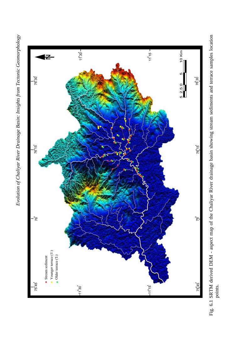
Sediment Sampling was restricted to the Nilambur valley area (Fig. 6.1).
Sediment samples were collected from the present day stream channel (T0), younger

Chapter VI: Sedimentology
198
terrace (T1) and older terrace (T2). Samples from still older terraces were avoided as the
terraces have been more or less lateritized.
All the sub samples were dried in hot air oven at 50ºC before they were
subjected to textural analysis. The samples represented three domains- stream sediment
and terrace samples T1 and T2. 32 stream sediment, 47 T1 and 28 T2 samples were
subjected to textural analysis. The weighed samples (approx. 100g) were treated with
15% H2O2 for removal of organic matter. Later the samples were heated up to 70ºC till
the effervescence stopped to remove the excess H2O2 present in the samples. The treated
samples are used for grain size analysis and major elements estimation. In total, 32
stream sediment samples, 47 samples from T1 terraces and 28 samples from T2 terrace
are collected and analyzed for texture and for major elements.
6.2.2 Textural analysis
The oven-dried samples were sieved through ASTM mesh wet sieves (6"
diameter) arranged at 0.5 intervals using mild water jet. Mud was thoroughly washed
from each sieve using distilled water. Fractions in the sieves were air-dried, weighed
and calculated the weight percentage and other statistical parameters following the
standard procedure (Folk and Ward, 1957). The mud (silt and clay) fraction obtained
after wet sieving is used for pipette analysis to estimate the silt and clay. The pipette
analysis was carried out at 1 interval up to 11 using the procedure as suggested by
Galehouse (1971). The sand-silt-clay percentages were plotted on a ternary diagram to
obtain different textural classes (Folk et al., 1970).
Generally four grain size parameters are used to describe the grain size
distribution. The grain size in phi values of the samples was plotted against the
cumulative weight percentage on a probability chart and different percentile values of
5, 16, 25, 50, 75, 84 and 95 ( ) were obtained from the graph and grain size parameters
viz., mean, standard deviation, skewness and kurtosis are calculated using Folk and
Ward’s formulae (1957).
Various bivariate plots have been prepared to discriminate different depositional
environments for all the sample types (Friedman, 1961; Tanner, 1991a,b). These
bivariate plots are prepared to examine their suitability to serve as discriminants for
identifying the dominant depositional processes and environment. The bivariate plots
Evo
luti
on o
f C
hali
yar
Riv
er D
rain
age
Basi
n:
Insi
ghts
fro
m T
ecto
nic
Geo
morp
holo
gy
Fig
. 6.1
SR
TM
der
ived
DE
M -
asp
ect
map
of
the
Chal
iyar
Riv
er d
rain
age
bas
in s
how
ing s
trea
m s
edim
ents
and t
erra
ce s
ample
s lo
cati
on
poin
ts.
Chapter VI: Sedimentology
200
prepared for the stream sediments and T1 and T2 terrace samples : Bivariate plots - (i)
mean size vs. standard deviation and (ii) standard deviation vs. Skewness iii) mean size
vs. skewness. (iv) Friedman’s plot, (v) Tanner’s plot (mean size vs. sorting) are
represented in Fig. 6.5 and 6.6. CM diagram is prepared and represented in Fig. 6.6a.
Friedman’s bivariate plot discriminates sands of beach and river environments.
Tanner’s bivariate plot differentiates the sediments based on the energy zone and
environment of deposition. It discriminates sands of fluvial, estuarine or closed basin
environment. The CM diagram is prepared (Passega, 1964; 1972) as it offers a platform
for the purpose of deducing transportation modes of sediments. The position of the
points in a CM diagram depends upon the mode of deposition of the sediments. The CM
diagram of the sediment samples were prepared to understand the
transportation/deposition processes.
6.2.3 Geochemical analysis
The mineralogical and bulk chemical composition of sedimentary rocks and
sediments are used to determine provenance, evaluate palaeoclimate and tectonic
activity and study of the evolution of crust (Condie, 1967; Wildeman and Condie, 1973;
Pettijohn, 1975; Mac Lennan and Taylor, 1982; Nesbitt and Young, 1982; Cullers et al.,
1988; Mac Lennan and Taylor, 1991; Potter, 1994).
Chemical weathering affects plagioclase preferentially, K-feldspar
comparatively and quartz least of all (Nesbitt and Young, 1989). The weathered residue
of feldspars is clay minerals. Feldspar depletion becomes progressively more
pronounced as weathering proceeds and resulting sandy sediment become progressively
less representative of the source rock.
The bulk chemical analysis of representative samples from stream (SS) and
terraces (T1 and T2) is carried by XRF method. In total, 10 stream sediment samples, 7
T1 terrace samples, and 7 T2 terrace samples are analyzed.
A-CN-K and A-CNK-FM diagrams
Chemical weathering of silicate rocks result in the rapid and continuous loss of
cations like Ca, Na, Mg and K, slow and variable loss of silica and gradual enrichment
of Al and Fe. The A-CN-K and A-CNK-FM diagrams are based on the molecular
concentration of Al2O3, CaO, Na2O, K2O, FeO and MgO in the sediment samples. From
the same molecular proportions, chemical index of alteration (CIA) is calculated:

Chapter VI: Sedimentology
201
CIA= 100)( 223232 100CaOOKONaOAlOAl
CIA value for average continental crust is about 50. Gibbsite and kaolinite have CIA
values of 100. CIA of sediment samples are good indicators of extent of chemical
weathering in the source area and therefore the climate conditions.
6.3 Results and Discussion
6.3.1 Texture
Textural distribution (Sand-silt-clay ratio)
The distribution pattern of the sand-silt-clay ratios of stream sediments, terrace
samples (T1 and T2) of the Nilambur valley area of the Chaliyar river basin is discussed
and compared.
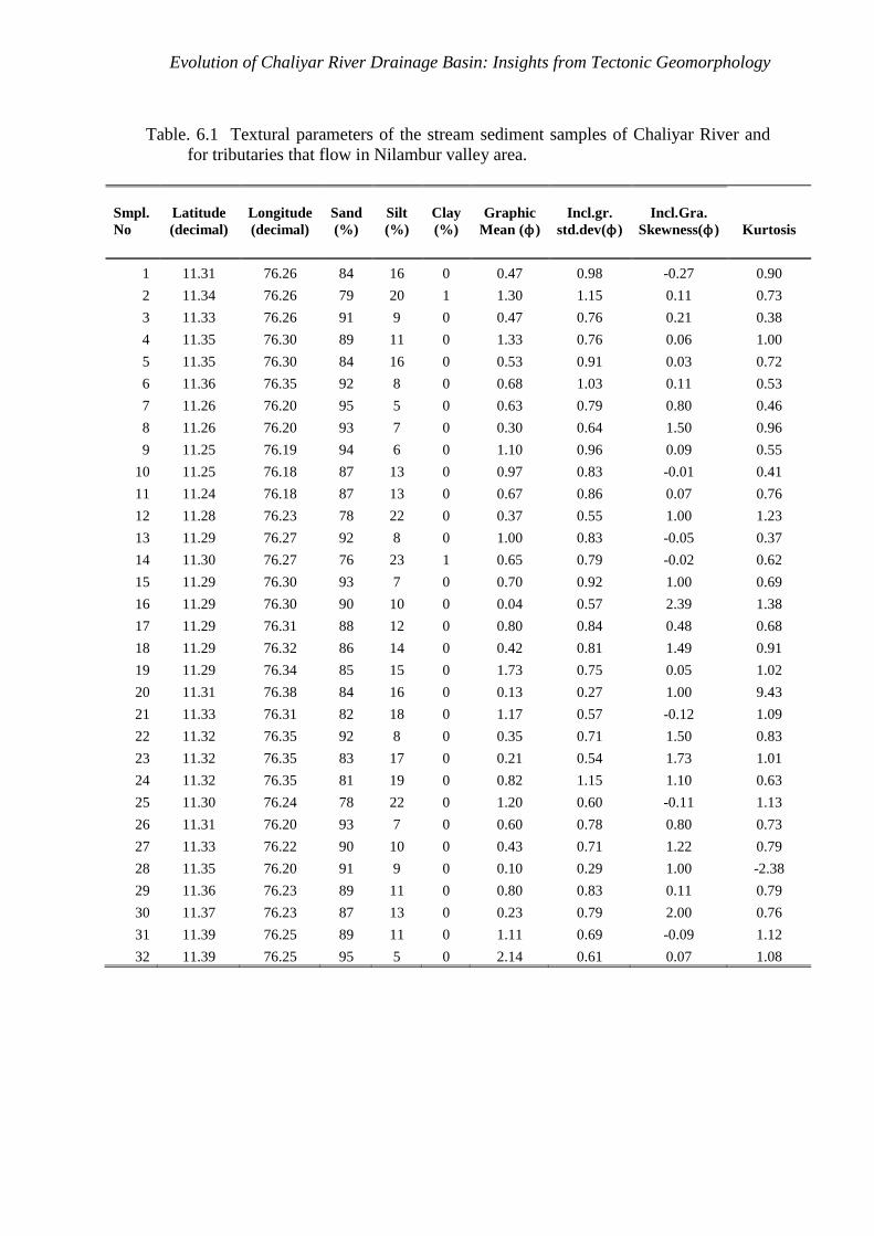
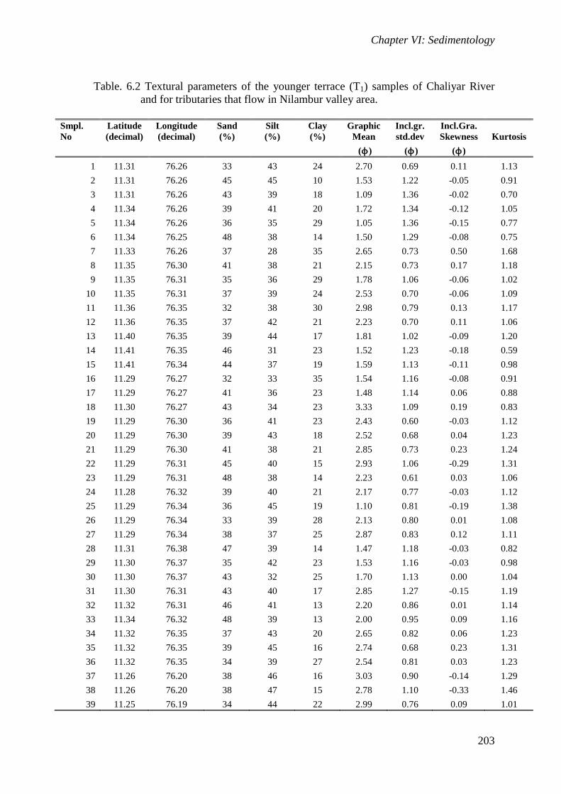
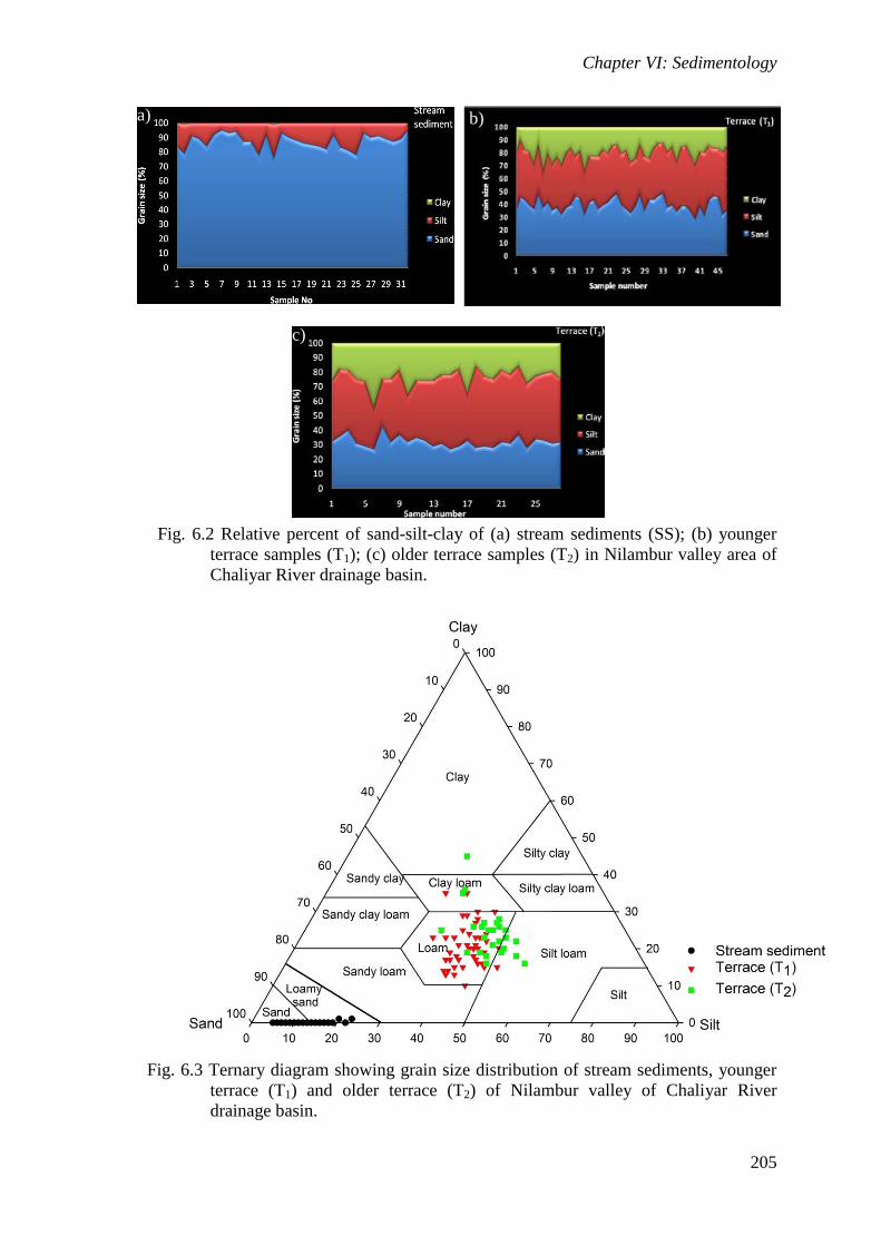
Sand content of stream sediments varies from 76-95% (average 87%), the silt
content from 5-23% (average 12.5%) and the clay content ranges from 0-1%. T1 terrace
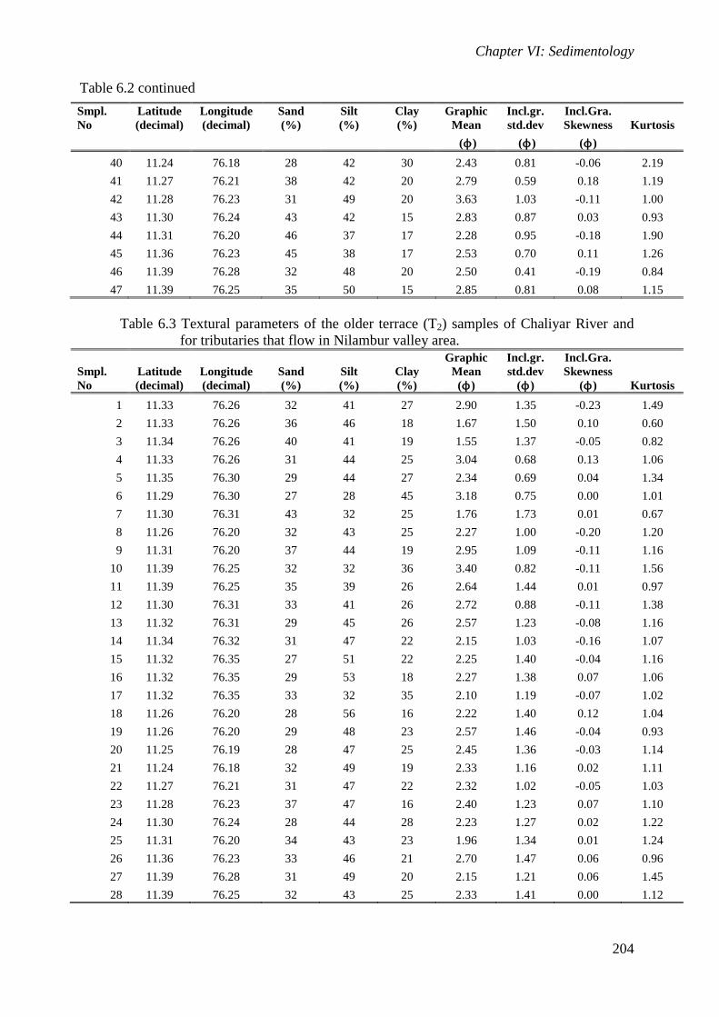
samples contain 28-48% of sand, 28-50% of silt and 10-35% of clay. Sand content in
T2 terrace samples ranges from 27-43%, silt content from 28-56% and clay content from
16-45% (Table 6.1, 6.2 and 6.3 and Fig.6.2 a, b and c).
The distribution of the sediments in ternary diagram of Sand–Silt–Clay after
USDA (Baize, 1988) in which stream sediments fall well within the sand and sandy
loam facies (Fig. 6.3). Loam is the dominant textural facies of both the terrace samples.
Grain size parameters The grain size parameters generally employed for the analysis of sediment size
distribution are mean (Mz), standard deviation ( 1), skewness (Sk1) and kurtosis (KG).
The mean size expresses the force of water, wind or current which can set the sediments
in motion. It is the reflection of the overall competency of the transportation dynamic
system (Goldbery, 1980). Standard deviation reflects the degree of sorting of the
sediment and depends on the range of the size of the sediment, rate of deposition and
strength and variation in energy of the agents of deposition. It allows an appreciation of
the size grading processes active during transport and deposition and reflects the energy
level in the environment of deposition (Lewis, 1984). Skewness indicates the degree of
symmetry and is a sensitive indicator of environment of deposition. It is controlled more
by the depositional processes than by the transporting conditions (Chamley, 1990).
Kurtosis is the degree of peakedness of a grain size frequency curve.
Evolution of Chaliyar River Drainage Basin: Insights from Tectonic Geomorphology
Table. 6.1 Textural parameters of the stream sediment samples of Chaliyar River and
for tributaries that flow in Nilambur valley area.
Smpl.
No
Latitude
(decimal)
Longitude
(decimal)
Sand
(%)
Silt
(%)
Clay
(%)
Graphic
Mean (ϕ)
Incl.gr.
std.dev(ϕ)
Incl.Gra.
Skewness(ϕ) Kurtosis
1 11.31 76.26 84 16 0 0.47 0.98 -0.27 0.90
2 11.34 76.26 79 20 1 1.30 1.15 0.11 0.73
3 11.33 76.26 91 9 0 0.47 0.76 0.21 0.38
4 11.35 76.30 89 11 0 1.33 0.76 0.06 1.00
5 11.35 76.30 84 16 0 0.53 0.91 0.03 0.72
6 11.36 76.35 92 8 0 0.68 1.03 0.11 0.53
7 11.26 76.20 95 5 0 0.63 0.79 0.80 0.46
8 11.26 76.20 93 7 0 0.30 0.64 1.50 0.96
9 11.25 76.19 94 6 0 1.10 0.96 0.09 0.55
10 11.25 76.18 87 13 0 0.97 0.83 -0.01 0.41
11 11.24 76.18 87 13 0 0.67 0.86 0.07 0.76
12 11.28 76.23 78 22 0 0.37 0.55 1.00 1.23
13 11.29 76.27 92 8 0 1.00 0.83 -0.05 0.37
14 11.30 76.27 76 23 1 0.65 0.79 -0.02 0.62
15 11.29 76.30 93 7 0 0.70 0.92 1.00 0.69
16 11.29 76.30 90 10 0 0.04 0.57 2.39 1.38
17 11.29 76.31 88 12 0 0.80 0.84 0.48 0.68
18 11.29 76.32 86 14 0 0.42 0.81 1.49 0.91
19 11.29 76.34 85 15 0 1.73 0.75 0.05 1.02
20 11.31 76.38 84 16 0 0.13 0.27 1.00 9.43
21 11.33 76.31 82 18 0 1.17 0.57 -0.12 1.09
22 11.32 76.35 92 8 0 0.35 0.71 1.50 0.83
23 11.32 76.35 83 17 0 0.21 0.54 1.73 1.01
24 11.32 76.35 81 19 0 0.82 1.15 1.10 0.63
25 11.30 76.24 78 22 0 1.20 0.60 -0.11 1.13
26 11.31 76.20 93 7 0 0.60 0.78 0.80 0.73
27 11.33 76.22 90 10 0 0.43 0.71 1.22 0.79
28 11.35 76.20 91 9 0 0.10 0.29 1.00 -2.38
29 11.36 76.23 89 11 0 0.80 0.83 0.11 0.79
30 11.37 76.23 87 13 0 0.23 0.79 2.00 0.76
31 11.39 76.25 89 11 0 1.11 0.69 -0.09 1.12
32 11.39 76.25 95 5 0 2.14 0.61 0.07 1.08
Chapter VI: Sedimentology
203
Table. 6.2 Textural parameters of the younger terrace (T1) samples of Chaliyar River
and for tributaries that flow in Nilambur valley area.
Smpl.
No
Latitude
(decimal)
Longitude
(decimal)
Sand
(%)
Silt
(%)
Clay
(%)
Graphic
Mean
Incl.gr.
std.dev
Incl.Gra.
Skewness Kurtosis
(ϕ) (ϕ) (ϕ)
1 11.31 76.26 33 43 24 2.70 0.69 0.11 1.13
2 11.31 76.26 45 45 10 1.53 1.22 -0.05 0.91
3 11.31 76.26 43 39 18 1.09 1.36 -0.02 0.70
4 11.34 76.26 39 41 20 1.72 1.34 -0.12 1.05
5 11.34 76.26 36 35 29 1.05 1.36 -0.15 0.77
6 11.34 76.25 48 38 14 1.50 1.29 -0.08 0.75
7 11.33 76.26 37 28 35 2.65 0.73 0.50 1.68
8 11.35 76.30 41 38 21 2.15 0.73 0.17 1.18
9 11.35 76.31 35 36 29 1.78 1.06 -0.06 1.02
10 11.35 76.31 37 39 24 2.53 0.70 -0.06 1.09
11 11.36 76.35 32 38 30 2.98 0.79 0.13 1.17
12 11.36 76.35 37 42 21 2.23 0.70 0.11 1.06
13 11.40 76.35 39 44 17 1.81 1.02 -0.09 1.20
14 11.41 76.35 46 31 23 1.52 1.23 -0.18 0.59
15 11.41 76.34 44 37 19 1.59 1.13 -0.11 0.98
16 11.29 76.27 32 33 35 1.54 1.16 -0.08 0.91
17 11.29 76.27 41 36 23 1.48 1.14 0.06 0.88
18 11.30 76.27 43 34 23 3.33 1.09 0.19 0.83
19 11.29 76.30 36 41 23 2.43 0.60 -0.03 1.12
20 11.29 76.30 39 43 18 2.52 0.68 0.04 1.23
21 11.29 76.30 41 38 21 2.85 0.73 0.23 1.24
22 11.29 76.31 45 40 15 2.93 1.06 -0.29 1.31
23 11.29 76.31 48 38 14 2.23 0.61 0.03 1.06
24 11.28 76.32 39 40 21 2.17 0.77 -0.03 1.12
25 11.29 76.34 36 45 19 1.10 0.81 -0.19 1.38
26 11.29 76.34 33 39 28 2.13 0.80 0.01 1.08
27 11.29 76.34 38 37 25 2.87 0.83 0.12 1.11
28 11.31 76.38 47 39 14 1.47 1.18 -0.03 0.82
29 11.30 76.37 35 42 23 1.53 1.16 -0.03 0.98
30 11.30 76.37 43 32 25 1.70 1.13 0.00 1.04
31 11.30 76.31 43 40 17 2.85 1.27 -0.15 1.19
32 11.32 76.31 46 41 13 2.20 0.86 0.01 1.14
33 11.34 76.32 48 39 13 2.00 0.95 0.09 1.16
34 11.32 76.35 37 43 20 2.65 0.82 0.06 1.23
35 11.32 76.35 39 45 16 2.74 0.68 0.23 1.31
36 11.32 76.35 34 39 27 2.54 0.81 0.03 1.23
37 11.26 76.20 38 46 16 3.03 0.90 -0.14 1.29
38 11.26 76.20 38 47 15 2.78 1.10 -0.33 1.46
39 11.25 76.19 34 44 22 2.99 0.76 0.09 1.01
Chapter VI: Sedimentology
204
Smpl.
No
Latitude
(decimal)
Longitude
(decimal)
Sand
(%)
Silt
(%)
Clay
(%)
Graphic
Mean
Incl.gr.
std.dev
Incl.Gra.
Skewness Kurtosis
(ϕ) (ϕ) (ϕ)
40 11.24 76.18 28 42 30 2.43 0.81 -0.06 2.19
41 11.27 76.21 38 42 20 2.79 0.59 0.18 1.19
42 11.28 76.23 31 49 20 3.63 1.03 -0.11 1.00
43 11.30 76.24 43 42 15 2.83 0.87 0.03 0.93
44 11.31 76.20 46 37 17 2.28 0.95 -0.18 1.90
45 11.36 76.23 45 38 17 2.53 0.70 0.11 1.26
46 11.39 76.28 32 48 20 2.50 0.41 -0.19 0.84
47 11.39 76.25 35 50 15 2.85 0.81 0.08 1.15
Table 6.3 Textural parameters of the older terrace (T2) samples of Chaliyar River and
for tributaries that flow in Nilambur valley area.
Smpl.
No
Latitude
(decimal)
Longitude
(decimal)
Sand
(%)
Silt
(%)
Clay
(%)
Graphic
Mean
(ϕ)
Incl.gr.
std.dev
(ϕ)
Incl.Gra.
Skewness
(ϕ) Kurtosis
1 11.33 76.26 32 41 27 2.90 1.35 -0.23 1.49
2 11.33 76.26 36 46 18 1.67 1.50 0.10 0.60
3 11.34 76.26 40 41 19 1.55 1.37 -0.05 0.82
4 11.33 76.26 31 44 25 3.04 0.68 0.13 1.06
5 11.35 76.30 29 44 27 2.34 0.69 0.04 1.34
6 11.29 76.30 27 28 45 3.18 0.75 0.00 1.01
7 11.30 76.31 43 32 25 1.76 1.73 0.01 0.67
8 11.26 76.20 32 43 25 2.27 1.00 -0.20 1.20
9 11.31 76.20 37 44 19 2.95 1.09 -0.11 1.16
10 11.39 76.25 32 32 36 3.40 0.82 -0.11 1.56
11 11.39 76.25 35 39 26 2.64 1.44 0.01 0.97
12 11.30 76.31 33 41 26 2.72 0.88 -0.11 1.38
13 11.32 76.31 29 45 26 2.57 1.23 -0.08 1.16
14 11.34 76.32 31 47 22 2.15 1.03 -0.16 1.07
15 11.32 76.35 27 51 22 2.25 1.40 -0.04 1.16
16 11.32 76.35 29 53 18 2.27 1.38 0.07 1.06
17 11.32 76.35 33 32 35 2.10 1.19 -0.07 1.02
18 11.26 76.20 28 56 16 2.22 1.40 0.12 1.04
19 11.26 76.20 29 48 23 2.57 1.46 -0.04 0.93
20 11.25 76.19 28 47 25 2.45 1.36 -0.03 1.14
21 11.24 76.18 32 49 19 2.33 1.16 0.02 1.11
22 11.27 76.21 31 47 22 2.32 1.02 -0.05 1.03
23 11.28 76.23 37 47 16 2.40 1.23 0.07 1.10
24 11.30 76.24 28 44 28 2.23 1.27 0.02 1.22
25 11.31 76.20 34 43 23 1.96 1.34 0.01 1.24
26 11.36 76.23 33 46 21 2.70 1.47 0.06 0.96
27 11.39 76.28 31 49 20 2.15 1.21 0.06 1.45
28 11.39 76.25 32 43 25 2.33 1.41 0.00 1.12
Table 6.2 continued
Chapter VI: Sedimentology
205
Fig. 6.2 Relative percent of sand-silt-clay of (a) stream sediments (SS); (b) younger terrace samples (T1); (c) older terrace samples (T2) in Nilambur valley area of Chaliyar River drainage basin.
Fig. 6.3 Ternary diagram showing grain size distribution of stream sediments, younger terrace (T1) and older terrace (T2) of Nilambur valley of Chaliyar River drainage basin.
a) b)
c)
Chapter VI: Sedimentology
206
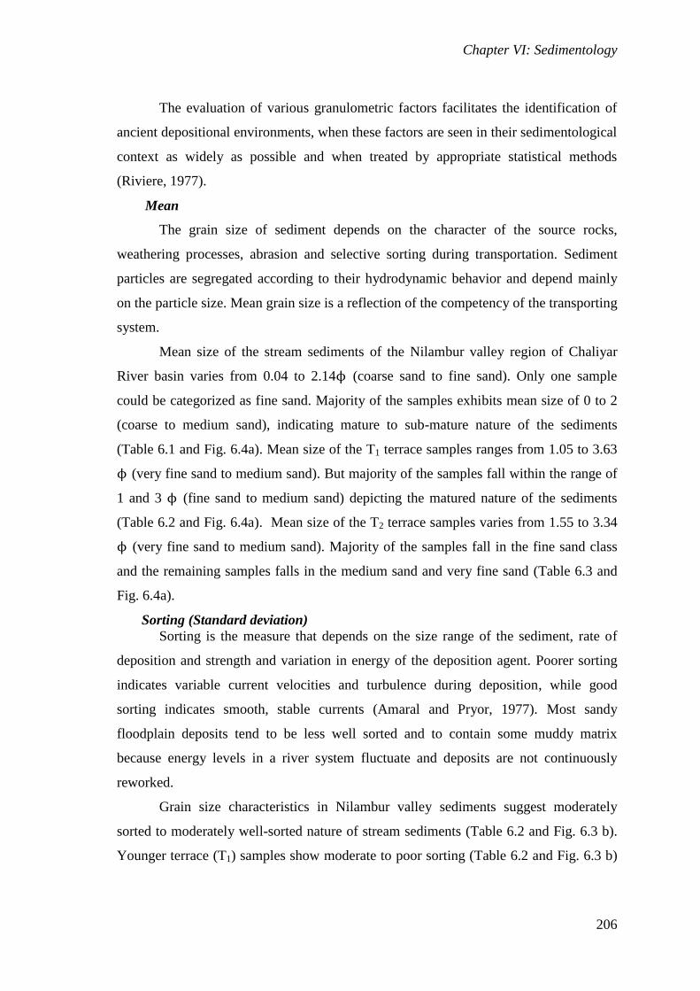
The evaluation of various granulometric factors facilitates the identification of
ancient depositional environments, when these factors are seen in their sedimentological
context as widely as possible and when treated by appropriate statistical methods
(Riviere, 1977).
Mean
The grain size of sediment depends on the character of the source rocks,
weathering processes, abrasion and selective sorting during transportation. Sediment
particles are segregated according to their hydrodynamic behavior and depend mainly
on the particle size. Mean grain size is a reflection of the competency of the transporting
system.
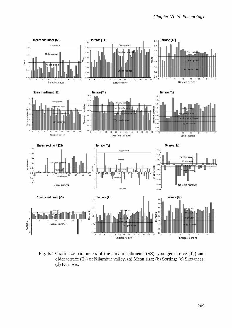
Mean size of the stream sediments of the Nilambur valley region of Chaliyar
River basin varies from 0.04 to 2.14ϕ (coarse sand to fine sand). Only one sample
could be categorized as fine sand. Majority of the samples exhibits mean size of 0 to 2
(coarse to medium sand), indicating mature to sub-mature nature of the sediments
(Table 6.1 and Fig. 6.4a). Mean size of the T1 terrace samples ranges from 1.05 to 3.63
ϕ (very fine sand to medium sand). But majority of the samples fall within the range of
1 and 3 ϕ (fine sand to medium sand) depicting the matured nature of the sediments
(Table 6.2 and Fig. 6.4a). Mean size of the T2 terrace samples varies from 1.55 to 3.34
ϕ (very fine sand to medium sand). Majority of the samples fall in the fine sand class
and the remaining samples falls in the medium sand and very fine sand (Table 6.3 and
Fig. 6.4a).
Sorting (Standard deviation)
Sorting is the measure that depends on the size range of the sediment, rate of
deposition and strength and variation in energy of the deposition agent. Poorer sorting
indicates variable current velocities and turbulence during deposition, while good
sorting indicates smooth, stable currents (Amaral and Pryor, 1977). Most sandy
floodplain deposits tend to be less well sorted and to contain some muddy matrix
because energy levels in a river system fluctuate and deposits are not continuously
reworked.
Grain size characteristics in Nilambur valley sediments suggest moderately
sorted to moderately well-sorted nature of stream sediments (Table 6.2 and Fig. 6.3 b).
Younger terrace (T1) samples show moderate to poor sorting (Table 6.2 and Fig. 6.3 b)
Chapter VI: Sedimentology
207
and majority of the older terrace (T2) samples exhibit poor sorting (Table 6.2 and Fig.
6.4 b).
Skewness
Skewness gives the degree of symmetry. Samples weighted towards the coarse
end-member are said to be positively skewed (lop-sided toward the negative phi values),
samples weighted towards the fine end are said to be negatively skewed (lop-sided
toward the positive phi values).Variation in the sign of skewness is due to varying
energy conditions of the sedimentary environments (Friedman, 1967). The river
sediments are usually positively skewed, beaches show a more normal distribution with
a slight positive or negative skew, and dune sands are invariably positive (Friedman,
1979). Positive skewness is due to the competency of the unidirectional flow of the
transporting media where the coarse end of the size frequency curve is chopped off
while negative skewness is caused by the amputation of the fine grained end of the
curve due to the winnowing action (Valia and Cameron, 1977). Winnowing action
produced by fluid media is the mechanism that gives negative skewness, whereas
sediments resulting from accumulation in sheltered environments are dominantly
positively skewed (Duane, 1964). Negatively skewed sediments are affected by higher
energy depositing agent, and are subjected to transportation for a greater length of time,
or the velocity fluctuation toward the higher values occurred more often than normal
(Sahu, 1964).
In Nilambur valley, 47% of the stream sediments are strongly positively skewed
and 30% of the samples show nearly symmetrical skewness, 4% are fine skewed and
only 9% of the samples are negatively skewed. Samples that show negative skewness
are from the seventh order main stream. Samples of the T1 terrace are dominantly near
symmetrical (51%). 25% of the samples are negatively skewed, and the remaining 24%
are negatively skewed. Majority of the T2 terrace samples exhibit near symmetrical
skewness (68%), 21% of the samples show negative skewness and the remaining 11%
are positively skewed (Table 6.2 and Fig. 6.4c).
Kurtosis
Kurtosis is the degree of peakedness of a grain size frequency curve. Curves that
are more peaked than normal distribution curve are termed leptokurtic; those which are
saggier than the normal are said to be platykurtic.
Chapter VI: Sedimentology
208
Stream sediments are mainly platykurtic to very platykurtic (31% and 28%
respectively), 25% of the samples are mesokurtic and remaining 16% falls within
leptokurtic to very leptokurtic. About 53% of the (T1) terrace samples are leptokurtic
(47%) and very leptokurtic (6%), 30% mesokurtic and 17% platykutic (15%) to very
platykurtic (2%). T2 terrace samples are mainly leptokurtic and mesokurtic (47%), 11%
comes within platykurtic to very platykurtic and 4% very leptokurtic (Table 6.2 and Fig.
6.4 d).
6.3.2 Bivariate plots
The bivariate plots of statistical measures and depositional environments of
grain size data serve as reliable tools for identifying mechanisms of deposition (Kukal,
1971; Al-Ghadban, 1990). Important and most utilized bivariate plots are mean vs.
sorting, mean vs. skewness, sorting vs. skewness as suggested by various researchers
(cf. Folk and Ward, 1957; Stewart, 1958; Sahu, 1964; Folk, 1966; Friedman, 1967;
Moiola and Weiser, 1968; Siemers, 1976; Chakrabarti, 1977; Erlich, 1983; McLaren
and Bowles, 1985). Chakrabarti (1977) has demonstrated the relationship between the
mean size and skewness characteristics, which helps in demarcating distinct grouping of
sediments. He suggests that the size parameters alone cannot effectively differentiate
environments particularly when the sediments are bimodal or polymodal in character.
Bivariate plots of mean vs. sorting, mean vs. skewness and sorting vs. skewness for
bulk samples of all the sediment samples are shown in Fig. 6.5a, b, c.
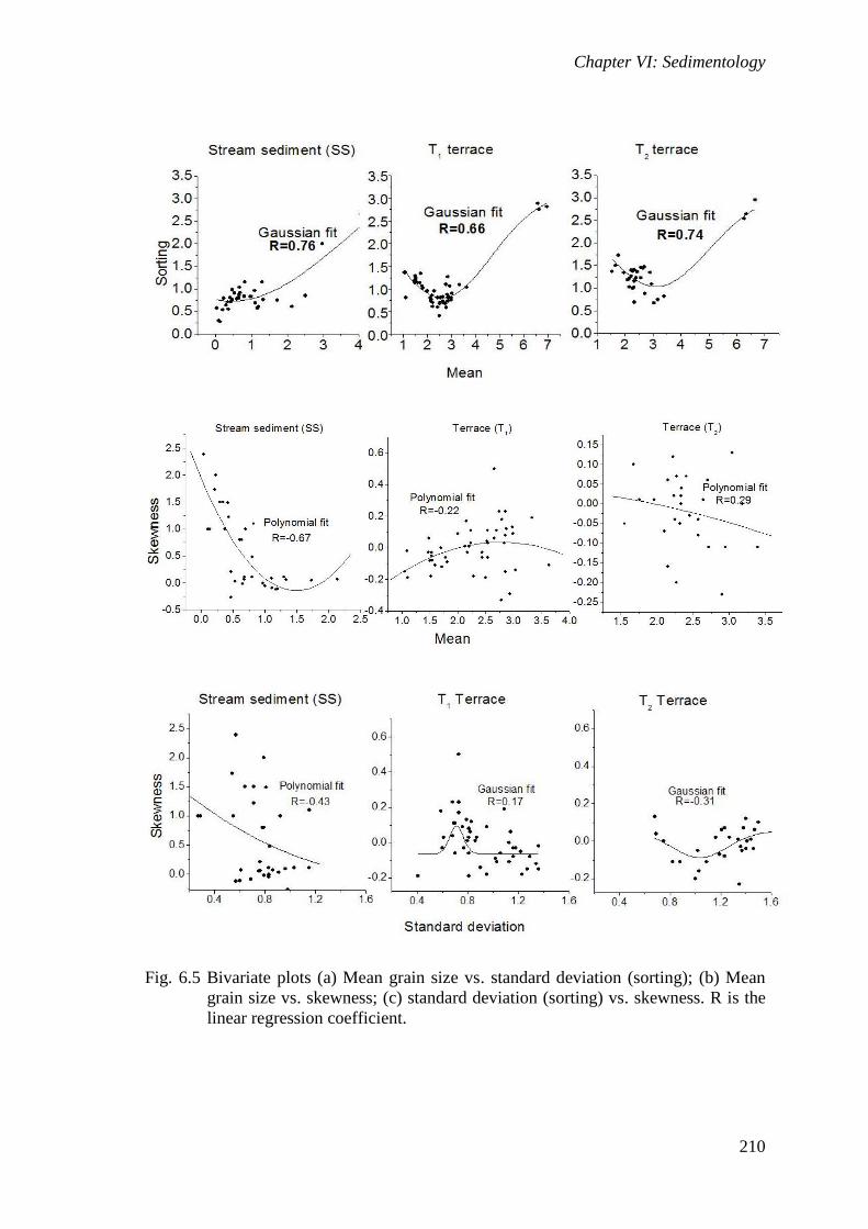
Graphic mean (Mz) vs. Inclusive graphic standard deviation (Sorting) (Graphic mean (Mz) vs. Inclusive graphic standard deviation (Sorting) ( 1)
Bivariate plot of mean vs. sorting (after Tanner, 1991) is plotted for stream
sediments and T1 and T2 terrace samples (Fig. 6.5). Very good positive correlation are
observed between mean and sorting for all the samples (R= 0.76 for SS, 0.66 for T1 and
0.74 for T2). Stream sediments and terrace samples show Gaussian fit distribution (Fig.
6.5a)
Mean (Mz) vs Skewness (Sk)
Samples from T1 terrace show slight positive correlation between mean size and
skewness. Stream sediments and T2 terrace samples show negative correlation (Fig.
6.5b). All the samples show polynomial fit sediment distribution (Fig. 6.5 b). Linear
Chapter VI: Sedimentology
209
Fig. 6.4 Grain size parameters of the stream sediments (SS), younger terrace (T1) and
older terrace (T2) of Nilambur valley. (a) Mean size; (b) Sorting; (c) Skewness;
(d) Kurtosis.
Chapter VI: Sedimentology
210
Fig. 6.5 Bivariate plots (a) Mean grain size vs. standard deviation (sorting); (b) Mean
grain size vs. skewness; (c) standard deviation (sorting) vs. skewness. R is the
linear regression coefficient.
Chapter VI: Sedimentology
211
regression coefficient (R) for stream sediment is -0.67 and that for T1 and T2 are -0.22
and 0.29 respectively (Fig. 6.5 b).
Sorting (Sorting ( 1) vs Skewness (Sk)
Bivariate plot shows that there is no correlation between these two parameters
( 1 and Sk) for any of the samples. Linear regression coefficient for stream sediment is
0.43, T1 is 0.17 and T2 is 0.31. Terrace samples (T1 and T2) show Gaussian distribution
while stream sediments show polynomial distribution (Fig. 6.5c).
6.4 Geochemistry Most primary minerals become thermodynamically unstable during the process
of weathering, erosion and transportation and alter to new stable secondary minerals by
physical disintegration and chemical weathering. Rock weathering process results in
grain size reduction, loss of soluble elements, enrichment of water insoluble elements
resulting in the formation of clay minerals. It is a continuous process, the rate and
intensity of which depend on the intensity of the physical variables on the surface,
topography, relief, structure, texture and geochemistry of the exposed rocks and time.
Geochemistry of the sediments helps to evaluate the nature of the provenance and
tectonic history of the provenance during sedimentation.
In this study, sediment samples from present day stream bed and terraces are
studied to understand the rate of weathering and thereby the chronological order of
deposition.
Major elements
Clastic sediments derived from the provenance area undergoing chemical
weathering of rocks show a similar compositional trend in the A-CN-K space. Some
chemical fractionation could occur during transport of sediment particles due to the
transportation of fine colloidal clay as suspended load. The extent of the transport
related geochemical fractionation depends on the extent of chemical weathering in the
provenance area. Any post depositional geochemical changes associated with
diagenesis/metasomatism of sediments can also be evaluated from these plots.
During the early stage of uplift of a terrain sediment supply become very
significant because of mass wasting and erosion. The sediments are physically and
chemically immature. As the net uplift rate decreases the degree of chemical weathering
increases and sediments become chemically evolved. However, the sediment deposited
Chapter VI: Sedimentology
212
finally bears the cumulative effect of tectonics and weathering history of the provenance
as well as reworking history during transit.
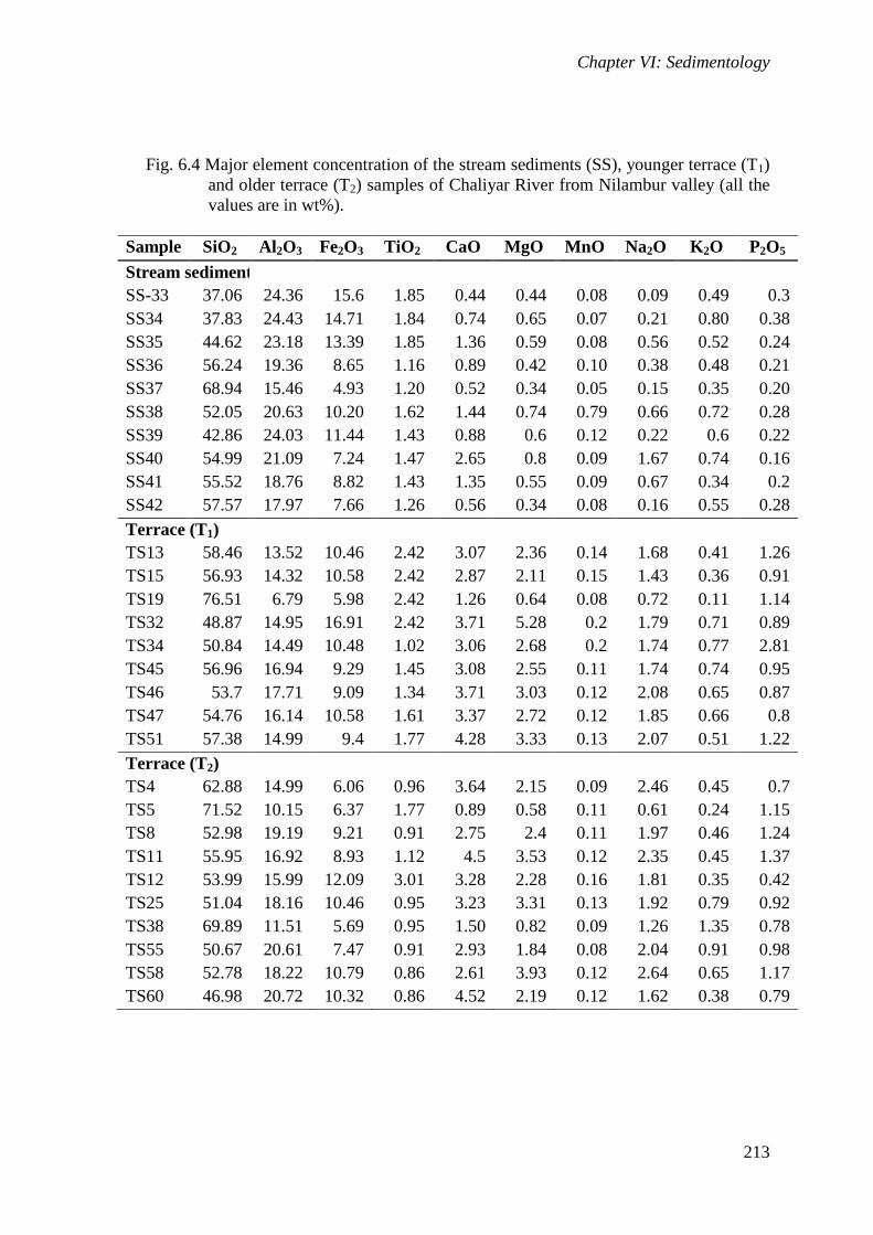
Major element concentration of the stream sediments and terrace samples (T1
and T2) are given in the Table. 6.5. A-CN-K diagram represents the molar proportion of
Al2O3, CaO+ Na2O and CaO, where CaO represents the part that has been derived from
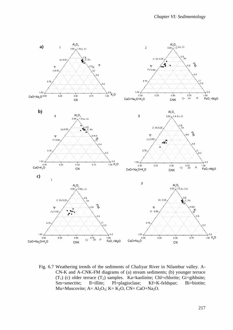
the silicate minerals (Nesbitt and Young, 1984; 1989). Within the A-CN-K
compositional space the plots of SS, T1 and T2 are close to the (A) Al2O3 apex showing
the concentration of alumina and potash (Fig. 6.6 a1, b1, c1). The sediments might have
derived from the charnockite and gneisses that form the hilly terrains of Chaliyar River
drainage basin. A-CN-K diagram for stream sediment shows highest concentration of
illite that has been derived from the K-feldspar. The preponderance of K-feldspar over
plagioclase also indicates the intensity of chemical weathering and alteration of
plagioclase to clay mineral (kaolinite).
A-CNK-FM plots show the molecular proportion of Al2O3, CaO+Na2O+K2O
and FeO (total) + MgO. Within the compositional space of A-CNK-FM diagram, the
plots for stream sediment samples and terrace samples are close to the feldspar A-CNK
zone close to feldspar apex (Fig. 6.6 a2, b2, c2). The plots of SS show their concentration
very close to the A apex indicating very high rate of chemical weathering. T1 and T2
terrace samples show almost similar characteristics and are concentrated towards the
feldspar apex. Intensity of chemical weathering is high in stream sediments than in
terrace sediments. The younger and older terraces (T1 and T2) do not show much
variation in the chemical characteristics as shown in plots of A-CN-K and A-CNK-FM
diagrams (Fig. 6.7). This suggests that the rate of chemical weathering is almost
uniform in both the deposits and the formation of these two terraces occurred within a
short span of time. However, formation of two levels of terraces within a short period of
time can only be explained by the signatures of tectonism.
The chemical index of alteration (CIA) has been widely used as a proxy for
chemical weathering in sediment source area (Nebitts and Young, 1982). It is commonly
used for characterizing weathering profiles. Chemical weathering indices incorporate
bulk major element oxide chemistry into a single value for each sample.
Chapter VI: Sedimentology
213
Fig. 6.4 Major element concentration of the stream sediments (SS), younger terrace (T1)
and older terrace (T2) samples of Chaliyar River from Nilambur valley (all the
values are in wt%).
Sample SiO2 Al2O3 Fe2O3 TiO2 CaO MgO MnO Na2O K2O P2O5
Stream sediment
SS-33 37.06 24.36 15.6 1.85 0.44 0.44 0.08 0.09 0.49 0.3
SS34 37.83 24.43 14.71 1.84 0.74 0.65 0.07 0.21 0.80 0.38
SS35 44.62 23.18 13.39 1.85 1.36 0.59 0.08 0.56 0.52 0.24
SS36 56.24 19.36 8.65 1.16 0.89 0.42 0.10 0.38 0.48 0.21
SS37 68.94 15.46 4.93 1.20 0.52 0.34 0.05 0.15 0.35 0.20
SS38 52.05 20.63 10.20 1.62 1.44 0.74 0.79 0.66 0.72 0.28
SS39 42.86 24.03 11.44 1.43 0.88 0.6 0.12 0.22 0.6 0.22
SS40 54.99 21.09 7.24 1.47 2.65 0.8 0.09 1.67 0.74 0.16
SS41 55.52 18.76 8.82 1.43 1.35 0.55 0.09 0.67 0.34 0.2
SS42 57.57 17.97 7.66 1.26 0.56 0.34 0.08 0.16 0.55 0.28
Terrace (T1)
TS13 58.46 13.52 10.46 2.42 3.07 2.36 0.14 1.68 0.41 1.26
TS15 56.93 14.32 10.58 2.42 2.87 2.11 0.15 1.43 0.36 0.91
TS19 76.51 6.79 5.98 2.42 1.26 0.64 0.08 0.72 0.11 1.14
TS32 48.87 14.95 16.91 2.42 3.71 5.28 0.2 1.79 0.71 0.89
TS34 50.84 14.49 10.48 1.02 3.06 2.68 0.2 1.74 0.77 2.81
TS45 56.96 16.94 9.29 1.45 3.08 2.55 0.11 1.74 0.74 0.95
TS46 53.7 17.71 9.09 1.34 3.71 3.03 0.12 2.08 0.65 0.87
TS47 54.76 16.14 10.58 1.61 3.37 2.72 0.12 1.85 0.66 0.8
TS51 57.38 14.99 9.4 1.77 4.28 3.33 0.13 2.07 0.51 1.22
Terrace (T2)
TS4 62.88 14.99 6.06 0.96 3.64 2.15 0.09 2.46 0.45 0.7
TS5 71.52 10.15 6.37 1.77 0.89 0.58 0.11 0.61 0.24 1.15
TS8 52.98 19.19 9.21 0.91 2.75 2.4 0.11 1.97 0.46 1.24
TS11 55.95 16.92 8.93 1.12 4.5 3.53 0.12 2.35 0.45 1.37
TS12 53.99 15.99 12.09 3.01 3.28 2.28 0.16 1.81 0.35 0.42
TS25 51.04 18.16 10.46 0.95 3.23 3.31 0.13 1.92 0.79 0.92
TS38 69.89 11.51 5.69 0.95 1.50 0.82 0.09 1.26 1.35 0.78
TS55 50.67 20.61 7.47 0.91 2.93 1.84 0.08 2.04 0.91 0.98
TS58 52.78 18.22 10.79 0.86 2.61 3.93 0.12 2.64 0.65 1.17
TS60 46.98 20.72 10.32 0.86 4.52 2.19 0.12 1.62 0.38 0.79
Chapter VI: Sedimentology
214
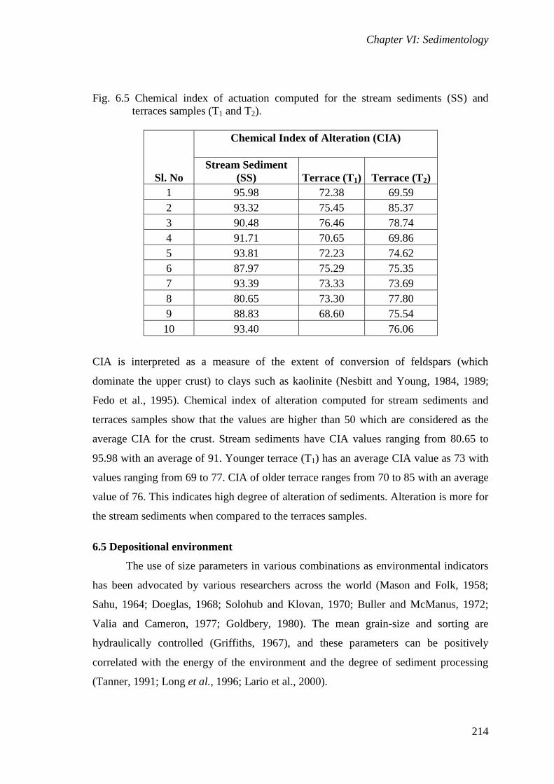
Fig. 6.5 Chemical index of actuation computed for the stream sediments (SS) and
terraces samples (T1 and T2).
Sl. No
Chemical Index of Alteration (CIA)
Stream Sediment
(SS) Terrace (T1) Terrace (T2)
1 95.98 72.38 69.59
2 93.32 75.45 85.37
3 90.48 76.46 78.74
4 91.71 70.65 69.86
5 93.81 72.23 74.62
6 87.97 75.29 75.35
7 93.39 73.33 73.69
8 80.65 73.30 77.80
9 88.83 68.60 75.54
10 93.40
76.06
CIA is interpreted as a measure of the extent of conversion of feldspars (which
dominate the upper crust) to clays such as kaolinite (Nesbitt and Young, 1984, 1989;
Fedo et al., 1995). Chemical index of alteration computed for stream sediments and
terraces samples show that the values are higher than 50 which are considered as the
average CIA for the crust. Stream sediments have CIA values ranging from 80.65 to
95.98 with an average of 91. Younger terrace (T1) has an average CIA value as 73 with
values ranging from 69 to 77. CIA of older terrace ranges from 70 to 85 with an average
value of 76. This indicates high degree of alteration of sediments. Alteration is more for
the stream sediments when compared to the terraces samples.
6.5 Depositional environment
The use of size parameters in various combinations as environmental indicators
has been advocated by various researchers across the world (Mason and Folk, 1958;
Sahu, 1964; Doeglas, 1968; Solohub and Klovan, 1970; Buller and McManus, 1972;
Valia and Cameron, 1977; Goldbery, 1980). The mean grain-size and sorting are
hydraulically controlled (Griffiths, 1967), and these parameters can be positively
correlated with the energy of the environment and the degree of sediment processing
(Tanner, 1991; Long et al., 1996; Lario et al., 2000).
Chapter VI: Sedimentology
215
CM diagram
Discussions of parameters C (first percentile of the size distribution) and M
(median of the size distribution in microns) showed that these parameters are indicators
of hydraulic conditions under which sediments were deposited (Passega, 2006). The C-
M plot (Passega, 1972) is used to understand the dominant mode of transportation and
the environment of deposition. C-M diagrams in which C is the one-percentile, M the
median of the grain-size distribution, characterize the coarsest fractions of the samples
(Passega et al., 2006). CM diagram gives the relationships which exist between certain
sizes of clastic grains and the most probable deposition mechanism are used to classify
clastic sediments by subdividing them into types indicative of their genesis.
First percentile of the size distribution (C) in microns was plotted against the
median of the size distribution in microns (M) for the stream sediments (SS) and T1 and
T2 terraces sediments (Fig. 6.6 a). It is observed that stream sediments are characterized
by the rolling process of deposition. T1 terrace samples are mainly deposited under
graded suspension and maximum grain size was transported by uniform suspension. T2
terrace samples are deposited by suspension with rolling process. Maximum grain size
of this terrace deposit was transported by graded suspension.
Friedman’s plot (Phi Sorting vs. Skewness)
In Friedman’s plot, standard deviation (sorting) is plotted against skewness as
suggested by Friedman (1961, 1967) to discriminate the sands of beach and river
environments (Fig. 6.6 b). About 90% of the terraces samples fall well within the fluvial
regime of the plot indicating the riverine origin of the terraces. Few stream sediments
fall within the beach profile (20%) and this may be due to the winnowing action of the
stream and variable current velocities in the higher order streams.
Tanner’s bivariate plot
Tanner (1991) proposed a bivariate plot of mean against standard deviation
(sorting) showing the high and low energy zones and fluvial and estuarine zones of
deposition. In this study, the parameter mean size of the sand fraction of the sediments
was plotted against sorting values (Fig. 6.6c). It shows that all the stream sediments and
majority of the terrace samples fall well within the fluvial and stream episode zone.
About 7% of the terrace samples fall in the fluvial estuarine/closed basin boundary.

Chapter VI: Sedimentology
216
Fig. 6.6 Plots of grain size parameters. (a) Depositional processes derived from CM diagram for stream sediments, and T1 and T2 terrace samples (after Passega, 1972); (b) Friedman’s (1961) bivariate plot of standard deviation (sorting)
vs. skewness applied for the sand fractions of the samples from the stream sediment (SS), and terraces of two levels (T1 and T2) of Chaliyar river; (c) Bivariate plot of mean size vs. sorting after Tanner, 1991) for stream sediments and terrace samples of Chaliyar River from Nilambur valley.
a)
b)
c)
b)
Chapter VI: Sedimentology
217
a)
b)
c)
1
1
2
2
12
2b)
1
2
Fig. 6.7 Weathering trends of the sediments of Chaliyar River in Nilambur valley. A-CN-K and A-CNK-FM diagrams of (a) stream sediments; (b) younger terrace (T1) (c) older terrace (T2) samples. Ka=kaolinite; Chl=chlorite; Gi=gibbsite; Sm=smectite; Il=illite; Pl=plagioclase; Kf=K-feldspar; Bi=biotite; Mu=Muscovite; A= Al2O3; K= K2O, CN= CaO+Na2O.
Chapter VI: Sedimentology
218
6.6 Summary
Stream sediments of the Chaliyar River and its tributaries in the Nilambur valley
area texturally consists of sand and sandy loam facies. Sandy sediments are moderately
well-sorted, matured to sub-matured, coarse- to medium grained. Loam is the dominant
textural facies for both younger and older terraces. Younger T1 terrace consists of
matured fine- to medium-grained sand that is moderate to poorly sorted. Older terrace
(T2) sediments are medium to fine- grained sand but are poorly sorted.
Statistical analysis of the grain size parameters are used to interpret depositional
environment and describe the changes in the environmental settings. Stream sediments
are positively skewed and its bivariate plot (Mz vs. σ1) suggests the flowing water
regime, exhibits polynomial fit. Plots of mean size against skewness also shows
polynomial fit for stream sediments. Sorting coefficient plotted against skewness for T1
and T2 terraces shows Gaussian fit. Mean grain size when plotted against skewness
shows positive correlation with polynomial fit for T1 samples and negative correlation
for T2 samples with polynomial fit.
From the bivariate plots of Tanner (1991) and Friedman (1961; 1967), it is
observed that the depositional environment of the stream sediments and terrace samples
is of episodic fluvial and stream regimes. Few T2 samples fall within the closed basin or
partially opened estuarine condition which can be explained by the localized ponding
that might have occurred during the time of deposition. CM plot (Passega, 1972) for
stream sediments typify the rolling of sediments during the depositional process.
Younger terrace samples (T1) were transported by uniform suspension and deposited by
graded suspension, while older T2 terrace samples were transported by rolling process
and deposited by suspension.
Geochemical data have helped in ascertaining the weathering trends of the
sediments. The chemical index of alteration (CIA) has been used to quantify the degree
of weathering of stream sediments and terraces samples. CIA values range between 68
and 96 on a scale of 40-100, indicating a high degree of alteration (stream sediments
seem to be more altered). Similar geochemical properties and rate of weathering of the
younger and older terraces indicate that there was no time gap between the time of
deposition of these two formations. It is understood that the formation of two levels of
terraces can take place at the same time due to tectonism.
Related Documents