CHAPTER THREE.doc

CHAPTER THREE - THEORY AND DESIGN

3.1 INTRODUCTION

The study of the microwave propagation theory is important in microwave communication

because it provides important properties of the microwave link upon which the feasibility of the

link depends. Some of the functions of the theory are as follows;

The propagation theory identifies the prediction models for estimating the power required

to establish reliable communications.

It gives clues to the receiver techniques for compensating the impairments introduced

during the transmission of signals.

The propagation effects and other signal impairments are often collected and estimated.

The communication channel is well study and investigated.

The various channel models for microwave communications are also defined in the

propagation theory. These models are the Physical models and Statistical Models.

In addition to propagation impairments, the other phenomena that limit microwave

communications are noise and interference. All of these phenomena are treated in the

propagation theory [13].

3.2 THE FREE SPACE PROPAGATION MECHANISM

Fig 3.0 A Typical Transmission System

Microwave transmission is characterized by the generation of the information signal from the

source. In the transmitter (TX), an electric signal representing the desired information is been

given the required amount of power required to propagate through the channel without

interference in a process called modulation. A highly sensitive receiver (RX) at the far end of

transmission estimates the transmitted information from the recovered electrical signal and

recreates the information that was transmitted in a process called demodulation. The antenna at

both the transmitting and receiving ends acts as a transducer which converts between electrical

signals and radio waves, and vice versa. The transmission effects are most completely described

by the Maxwell’s equations as well as the Friis transmission equations. Here we assume a linear

medium in which all the distortions can be characterized by attenuation or superposition of

different signals [14].

3.3 COMMUNICATION NETWORKING

Communication Networking is the arrangement of hardware and software that allows users to

exchange information. It is one of the fastest growing areas in electrical engineering [15].

The type of communication networks includes;

Telephone network

Computer network

Cellular telephone networks

Television broadcast networks

Internet.

3.4 MECHANISM OF RADIO WAVE PROPAGATION.

The mechanism of radio wave propagation considers the exact physics of the propagation

environment (site geometry). It provides reliable estimates of the propagation behaviour. Some of

the basic mechanisms of propagation of radio waves include; Reflection, Refraction, Diffraction,

line of sight, Ducting, Scattering etc [13].

Wireless communication networking is achieved through electromagnetic wave (radio)

propagation. This ranges from short distance to very long distance propagation. An example of

short distance propagation is infrared and blue tooth and that of long distance is the microwave.

There are different nodes in long distance radio propagation. They are [13]

Sky wave propagation

Ground wave propagation

Space wave propagation

3.5 FREE SPACE PATH LOSS

The free space propagation model assumes a transmit antenna and a receive antenna to be located

in an otherwise empty environment, neither absorbing obstacles nor reflecting surfaces

considered. The influence of the earth surface is assumed to be entirely absence. For a

propagation distance much larger than the antenna size, the far field electromagnetic wave

dominates all other components. We model the radiating antenna as a point source with neglible

physical dimension; hence the energy radiated by the Omni-directional antenna is spread over the

surface of a sphere. This helps to analyze the effect of distance on the received signal power [8].

If the surface area of the sphere of radius ; then the power density at that distance with

transmit power and antenna gain is given as;

Then the available power at the receiving antenna with is given as

Where; = effective area (aperture) of the antenna and , the product of transmit

power and antenna gain at the transmitter is known as the effective radiated power at the

transmitter [8].

Consider a signal transmitted through free space to a receiver located at a distance Km from the

transmitter. Assume there are no obstruction between the transmitter and the receiver and that the

signal propagates along a straight line between the two. The channel model associated with this

transmission is called a line – of- sight channel, and the corresponding received signal is called

ray. Free space path loss introduces a scale factor resulting in the received signal [8];

;

Where is the product of transmit and the receive antenna field radiation pattern in the LOS

direction. The phase shift is due to the distance that the waves travel. The power in the transmitted

signal S (t) is , so the ratio of received power to the transmitted power from the above equation

is

Thus the received signal power falls off in the inverse proportion to the square of the distance

between transmit and received antenna [8].

3.6 SOME TERMINOLOGIES AND DEFINITIONS IN MICROWAVE LINK DESIGN.

Microwave design is not a one step procedure but involves better understanding of the

electromagnetic theory and other terminologies. Some terminologies and technologies associated

with the microwave design that will help in better understanding of the project are explained

below.

3.6.1 Free Space Loss: As signals spread out from a radiating source, the energy is spread out

over a larger surface area. As this occurs, the strength of that signal gets weaker. Free space loss

(FSL), measured in dB specifies how much the signal has weakened over a given distance. The

type of antenna used has no effect on FSL, since at any appreciable distance all antennas look like

a point source radiator. The area that the signal spreads out into is called the Fresnel zone. If there

is an obstacle in the Fresnel zone, part of the radio signal will be diffracted or bent away from the

straight-line path. The practical effect is that on a point-to-point radio link, this refraction will

reduce the amount of RF energy reaching the receive antenna. The thickness or radius of the

Fresnel zone depends on the frequency of the signal — the higher the frequency, the smaller the

Fresnel zone [5].

3.6.2 Receive signal level: This is the actual received signal level (usually measured in negative

dBm) presented to the antenna port of a radio receiver from a remote transmitter [5].

3.6.3 Receiver sensitivity: This is the weakest RF signal level (usually measured in negative

dBm) that a radio needs receive in order to demodulate and decode a packet of data without errors

[5].

3.6.4 Antenna gain: This is the ratio of how much an antenna boosts the RF signal over a

specified low-gain radiator. Antennas achieve gain simply by focusing RF energy. If this gain is

compared with an isotropic (no gain) radiator, it is measured in dBi. If the gain is measured

against a standard dipole antenna, it is measured in dBd. Note that gain applies to both transmit

and receive signals [5].

3.6.5 The Transmit Power: This is the RF power coming out of the antenna port of a transmitter.

It is measured in dBm, Watts or milliWatts and does not include the signal loss of the coax cable

or the gain of the antenna [5].

3.6.6 Effective Isotropic Radiated Power (EIRP): This is the actual RF power as measured in the

main lobe (or focal point) of an antenna. It is equal to the sum of the transmit power into the

antenna (in dBm) added to the dBi gain of the antenna. Since it is a power level, the result is

measured in dBm. The figure below shows how a 24dBm power can be boosted to 48dbm [5].

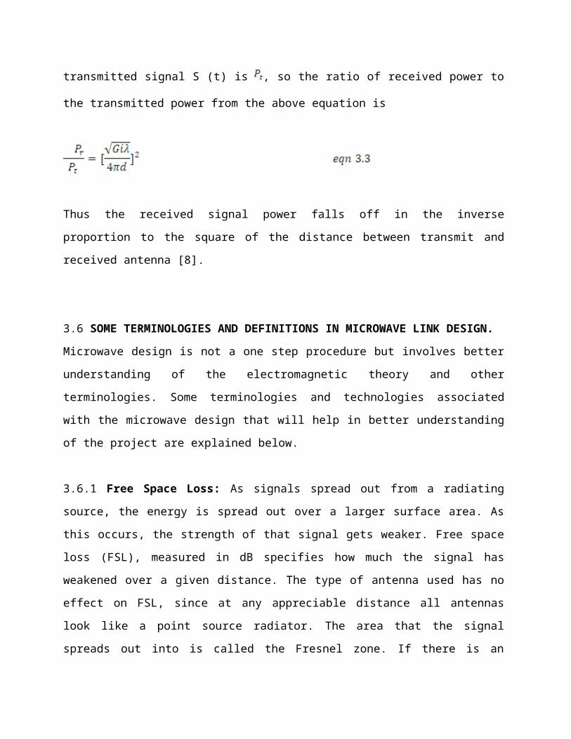
Fig 3.4 Effective Isotropic Radiated Power

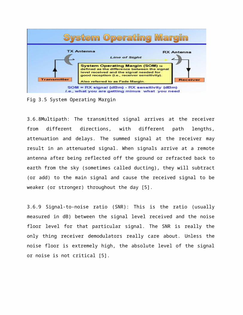
3.6.7 System Operating Margin (SOM):This is the difference (measured in dB) between the

nominal signal level received at one end of a radio link and the signal level required by that radio

to assure that a packet of data is decoded without error. SOM is the difference between the signal

received and the radio’s specified receiver’s sensitivity. SOM is also referred to as link margin or

fade margin [5].

Fig 3.5 System Operating Margin

3.6.8Multipath: The transmitted signal arrives at the receiver from different directions, with

different path lengths, attenuation and delays. The summed signal at the receiver may result in an

attenuated signal. When signals arrive at a remote antenna after being reflected off the ground or

refracted back to earth from the sky (sometimes called ducting), they will subtract (or add) to the

main signal and cause the received signal to be weaker (or stronger) throughout the day [5].

3.6.9 Signal-to-noise ratio (SNR): This is the ratio (usually measured in dB) between the signal

level received and the noise floor level for that particular signal. The SNR is really the only thing

receiver demodulators really care about. Unless the noise floor is extremely high, the absolute

level of the signal or noise is not critical [5].

3.6.10 Path Loss: Path loss is the loss of power of an RF signal travelling (propagating) through

space. It is expressed in dB. Path loss depends on: The distance between transmitting and

receiving antennas, line of sight clearance between the receiving and transmitting antennas and

antenna height [5].

3.7 LINK BUDGET FOR THE MOBILE SYSTEM

A link budget is a method of calculation used to determine the signal strength that a receiver will

receive from a transmitter located some distance away. In the GSM environment, it is critical to

balance the link budget on the uplink and downlink. Different coverage on the uplink and

downlink results in the dissipation of unnecessary energy resulting in increased interference to

other users in the network, increased costs and increased handover failures [16].

The factors affecting the link budget will be reviewed and link budgets will be determined for

various operating scenarios. These link budgets will be developed using spreadsheets [16].

The scope to be determined in the link budget includes [17];

Coverage Area; Definition, % Coverage

Propagation into and within Buildings

Transmission Feeder Loss Table.

Some factors affecting the link budget for a mobile system are as follows [16];

Receive Sensitivity: The sensitivity of the receiver of either the base station or the mobile

phone in dBm.

Feeder Loss: The attenuation of the amplitude of the radio frequency signal over the

length of the co-axial cable, measured in dB.

Mast Head Amplifier (MHA) Gain: The gain of an amplifier situated at the top of a mast,

measured in dB. This value should reflect the improvement in system sensitivity due to

the introduction of the MHA.

Antenna Gain: The amount of gain an antenna has relative to an isotropic radiator,

measured in dBi.

Diversity Gain: The gain in the received signal strength by using multiple antennas

separated from each other either in space or in polarity to overcome fading, measured in

dB.

Duplexer Loss: The loss associated with the insertion of a duplexer in the transmit and

receive path of the antennas, measured in dB.

Splitter Loss: The loss associated with the insertion of a splitter in the transmit and

receive path of the antennas, measured in dB.

Output Power: The power transmitted by the base station or the mobile phone, measured

in dBm.

Fade Margin: The margin introduced to overcome the fact that the received radio signal is

destructively interfered due to reflections off objects near the vicinity of the receiver,

measured in dB.

Frequency Hopping Gain: The gain introduced by frequency hopping due to reduced

interference in the network.

Path Loss: Attenuation of the radio signal due to propagation losses.

Slant Polarization Loss (Downlink path): due to difference in propagation

characteristics. (Only downlink, as uplink loss is taken into account by reducing the

polarization diversity gain).

3.7.1 TYPICAL VALUES OF FACTORS AFFECTING THE FADE MARGIN

As can be seen from appendix A, the feeder loss can vary according to the type of feeder and the

length of feeder used. The feeder loss generally also takes into account any loss through

connectors, which, depending on the type of antenna configuration used, may vary from 5 to 9

connectors. The loss through connectors could be taken as a separate entity.Transmission Feeder

Loss Table, can be used to determine the values for feeder losses to be used in link budget

calculations. The connector losses have been included in the figures used for the feeder losses

[16]

3.7.2 SHADOW FADE MARGIN

The shadow fading margin of 9.7 dB ensures better than 95% probability of coverage averaged

across the entire area of the cell, given a standard deviation of fading of 9 dB. Shadow fading

margins for different values of standard deviation may be obtained from appendix B, which was

developed by integration across the cell area. The numbers are based on a sectorized

configuration, but figures for the Omni directional case will be similar. For the indoor case, a

median building penetration loss of 14 dB and standard deviation of fading of 12 dB have been

applied, resulting in an additional margin of 18.4 dB for indoor coverage. Suggested values of

fade margin as given by Mercury One-2-One for different environment types are given in the

table below [18]:

Dense-

suburb

Urban-

sec

Urban-

Omni

Suburb-

sec

Suburb-

Omni

Rural-

sec

Rural-

Omni

Units

Fade

Margin

8.39 9.47 5.97 13.56 10.06 14.20 10.70 dB

Table 3.0 Typical Values of Fade Margin for Different Environments

3.7.3 RADIO BASE STATION OUTPUT POWER

The maximum power output of the different types of RBSs varies according to the configuration

employed. The output power of a RBS 2000 with a CDU-A is 2.5 dB higher than a RBS 200. The

loss between the transmitter and the antenna connector on the RBS 2000 with a CDU-C is 5 dB.

The loss between the transmitter and the antenna connector on the RBS 200 is 5 dB. To balance

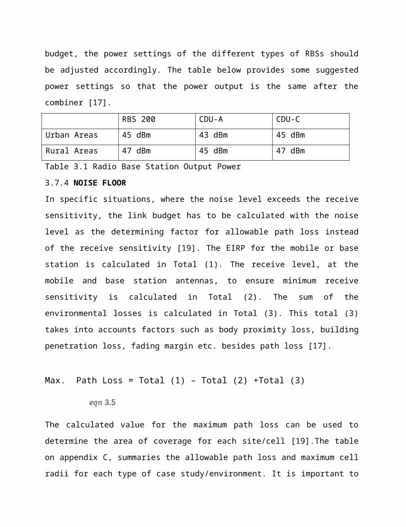
the link budget, the power settings of the different types of RBSs should be adjusted accordingly.

The table below provides some suggested power settings so that the power output is the same

after the combiner [17].

RBS 200 CDU-A CDU-C

Urban Areas 45 dBm 43 dBm 45 dBm

Rural Areas 47 dBm 45 dBm 47 dBm

Table 3.1 Radio Base Station Output Power

3.7.4 NOISE FLOOR

In specific situations, where the noise level exceeds the receive sensitivity, the link budget has to

be calculated with the noise level as the determining factor for allowable path loss instead of the

receive sensitivity [19]. The EIRP for the mobile or base station is calculated in Total (1). The

receive level, at the mobile and base station antennas, to ensure minimum receive sensitivity is

calculated in Total (2). The sum of the environmental losses is calculated in Total (3). This total

(3) takes into accounts factors such as body proximity loss, building penetration loss, fading

margin etc. besides path loss [17].

Max. Path Loss = Total (1) – Total (2) +Total (3)

The calculated value for the maximum path loss can be used to determine the area of coverage for

each site/cell [19].The table on appendix C, summaries the allowable path loss and maximum cell

radii for each type of case study/environment. It is important to note that the cell radii are reduced

for indoor coverage (900 MHz) and for outdoor coverage at 1800 MHz as compared to outdoor

coverage at 900MHz. The allowable path loss in each case study is the lower of the allowable

uplink and downlink values as calculated in the case studies. The maximum cell radius is as

calculated by the Okumura Hata propagation model [17].

3.8 THE NETWORK DESIGN OBJECTIVES AND ANALYSIS

Radio link engineering begins by performing the link budget analysis. A given radio system has a

system gain that depends on the radio and the type of modulation used. The gains from the

antenna at both ends are added to this gain. The free space loss of the radio signal as it travels

over the air is subtracted from the system gain. These calculations results in a fade margin for the

link. Anything that affects the radio link signal within this margin will be overcome by the radio;

if the margin is exceeded, the link could go down. The next step is to analyze impediments that

could potentially affect the radio signal. The goal is to get availability and performance [4].

The objective is to design a communication network for Bui City which is suitable for both voice

and data communication. In particular, the design is to

Connect Bui City to the Tigo network through Banda Ahenkro .

Flexibility, allowing for future expansion without any major changes of the network to

other communities and locations.

Make possible the provision of service comparable in technical quality and availability

with that in areas of normal mobile density.

Allow the network to be operated at a minimum operating cost.

3.8.1 THE MICROWAVE NETWORK DESIGN STRATEGY

Point-to-point microwave communications systems operating on a “line-of-sight” (LOS) basis are

subjected to predictable propagation-related performance characteristics; they must neither cause

nor suffer objectionable RF interference with other systems using the same frequencies, and

requires an NCA license to be operated. Microwave network design follows some sequential steps

in its implementation, these steps includes:

Identification of Communications Requirements: What points need to be connected, with

what capacity, and with what level of performance? This is where the points of

communication and the required capacity between the transmitting and receiving ends are

identified. The factors that affect the capacity of the channel include; the population,

number of co-operate institutions like financial institutions, schools, service proposed, etc.

[5].

Selection of System Type: This step deals with the selection of a frequency band and type

of system. The distance between points of communication determines the usable

frequency bands, as propagation characteristics of different frequency bands (combined

with available technologies) effectively subject them to different maximum practical link

lengths. Capacity requirements also determines frequency band, as the channelization and

maximum bandwidths allowed in different bands effectively set maximum per-channel

and system capacity [5].

Site Selection and Route Design: The purpose of the site selection and route design is to

provide at least a preliminary network layout to start the engineering work. The important

data that are needed in this process are the points of communication, frequency band,

possible limitations on antenna heights placement, type of antenna lines, etc. The main

process is connecting the various nodes in the communication link in a manner so as to

minimise the necessary number of links. After the process, the site location, possible route

layout and the various limitations are the output of this process. The coordinates of the

points of communication are critical to the work that follows after this procedure [5].

Preliminary Path Profiling: The purpose of this step is to determine, at least on a

preliminary basis, whether the links between specified points are feasible, based on early

estimates of necessary antenna heights to achieve line-of-sight. It is also done to identify

critical points along the path that require on-site inspection to accurately determine the

existence and height of potential obstructions over which the path must pass. The data that

are used in this process are the portion of communication identified by the latitude and

latitude taken during the field survey and the frequency band selected. Within the process,

the path profile which is the vertical-plane graphical representation of each link to show

the height of the terrain and assumed natural obstructions along the path. The terrain

elevation data comes from digitized maps. The antenna heights are also set to provide

appropriate path clearance over those potential obstructions. The output of this step is the

preliminary antenna heights as well as the identification of critical locations on the path

where the path clearance needed to be set with the accurate information on obstruction

heights [5].

Field Path Surveys: In order to collect real world information on obstruction heights so

that the final antenna height can be set to provide appropriate path clearance, the field path

survey is carried out. The input data that are used during this procedure are the initial path

profile and a route layout showing all the end points noted along the path. Within the

process, the field crew examines the end points critically to confirm the coordinates as

well as other information about the sites and then drives along the path to collect data on

existence and heights of both natural and man-made obstructions, paying special attention

to critical points identified in the initial path profiling. Photographs are typically taken of

critical obstructions. Cautions must be taken since if the coordinates and other site

information are not entirely accurate, it means this procedure needs to be conducted again

[5].

Final Path Profiling: The purpose is to set the final antenna heights. The input data

required in this process are the preliminary path profile and the results of the field path

survey. The preliminary path profile is modified to incorporate real world obstruction

height data and the antenna centrelines are set to provide appropriate path clearance. The

final path profile and antenna centreline heights are the output to this procedure. One thing

to note is that field path surveys are the best way to a secure proper line of sight clearance

[5].

Path Propagation Performance Analysis: To determine whether performance of the

network will meet expectations or the path technical parameters should be modified or the

network necessarily is re-designed to meet the specified performance criterion, the path

propagation performance analysis is carried out. The input data to this step includes the

path length, frequency band and system technical data such as transmitter power, antenna

gain, antenna line loss, noise threshold etc. as well as specified link and network

performance criterion. Theses inputs are fed into standard formulas used to predict link

availability. If the specified per link performance criterion is not met, it is possible that the

combination of links still meet the overall network performance criterion. Antenna space

diversity or larger antennas may help meet the per link criterion. Frequency bands are

affected by the rainfall pattern and hence care should be taken to avoid link failure due to

rain attenuation [5].

RF Interference Analysis and Channel Selection: To determine whether interference free

(interference levels are within the acceptable limits) are available and sufficient number of

them to satisfy the capacity requirement is the purpose of this stage. During this stage, the

information necessary for the next step ,that is, NCA required prior coordination

notification are also gathered. The input data that are needed during this stage are the

station locations (lat/long), ground elevation, respective antenna types and antenna

centrelines, frequency band, transmitter power, receiver interference threshold which is

based on the channel capacity and equipment types. The above data are fed into

computerized interference analysis programs and the databases of system using the same

frequency band, interference levels are calculated and the comparisons made to standard

interference protection objectives. Possible changes in intended antennas to avoid

interference problems by using better radiation pattern and identification of interference

free channels are the outputs to this procedure [5].

Prior Frequency Coordination Notification and Response: Prior coordination notifications

(PCN’s) must be distributed to the operators of all other systems that shares the same

frequency band within the coordination distance of up to about 250miles for microwave

systems. This is done to satisfy NCA requirement for frequency coordination and to obtain

assurance of non-interference with other systems in the area. NCA licensing cannot be

obtained if this step is not completed [5].

NCA Licensing: When the PCN’s are received with positive response from other system

operators within the coordination area, the NCA issues authorization to operate the

system. The Environmental Protection Agency (EPA) also surveys the station locations to

check on possible treat on human settlement before NCA can issue the license based on

their recommendations [5].

The process is designed to work smoothly and efficiently. Experience, however, shows that

occasionally one or more steps in the process result in a “no go”, and portions of the work have to

be repeated. That is actually a normal (and effective) part of the process, and indeed the sequence

of steps is designed to either smoothly go from start to finish successfully, or at least obtain a

legitimate “no go” result as cost-effectively as possible. In other words, if a plan is eventually

going to be determined to be infeasible, it’s better to find out as early as possible. First, if input

data is not accurate, work (and money) will be wasted; take the time to avoid the “garbage in,

garbage-out” syndrome. Second, if there are unnecessary “rushes to judgment” and the normal

sequence is not followed, the overall engineering costs will likely be much higher than they could

have been, as portions of the process are necessarily repeated. Remember that the process

sequence is designed to deliver critical information to each successive step. When the steps are

taken in order and no roadblocks are encountered, the time is well spent [5].

3.8.2 THE COMMUNICATION REQUIREMENTS

The Bui Municipality with a population of about 90,023 in 2009 and an estimated population of

about 120,713 in 2014 having about 12,627 households. In designing a microwave network for

such a community to serve ICT purposes such as connectivity both in mobile and internet

services, free to air television systems, by taking the capacity requirement, estimated subscriber-

base as well as future projections into account, we will require a PDH radio system with capacity

of about 16E1’s which achieves high level of integration to provide cost, performance and

reliability and a performance level of about 99.999% where the level of network failure is very

small so as to solve the lower signal strength in the MTN network.

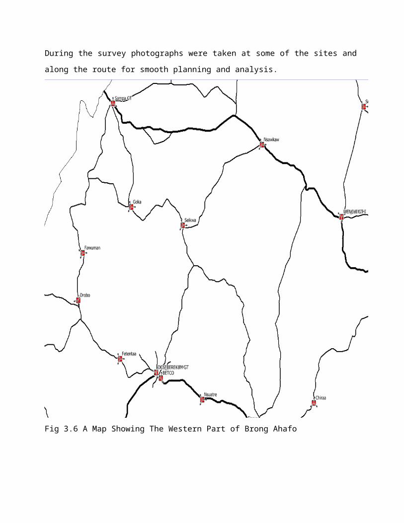
3.8.3 THE LAND TOPOLOGY SHOWING WESTERN PART OF BRONG AHAFO

Maps are the principal sources of basic data, both for office study which usually precedes the field

survey, and for the field survey itself. They show all information which will be necessary for

plotting of the path and also major aerial obstructions and large topographical feature such as

lakes and mountain ranges. If the terminal locations are plotted on an appropriate topo-map and

intermediate site are spliced in, an overall view of the possible route is obtain. As the map survey

proceeds, the preferred and ultimate sites arrived at by profiling. Other maps can be plotted using

the precise latitude and longitude [10].

The figure 3.3 shows the area map which was extracted from the digital microwave planning tool

kit. A visit to all sites selected for field survey, field strength test and determination of path profile

was conducted in all subsequent work in this project.

During the survey photographs were taken at some of the sites and along the route for smooth

planning and analysis.

Fig 3.6 A Map Showing The Western Part of Brong Ahafo

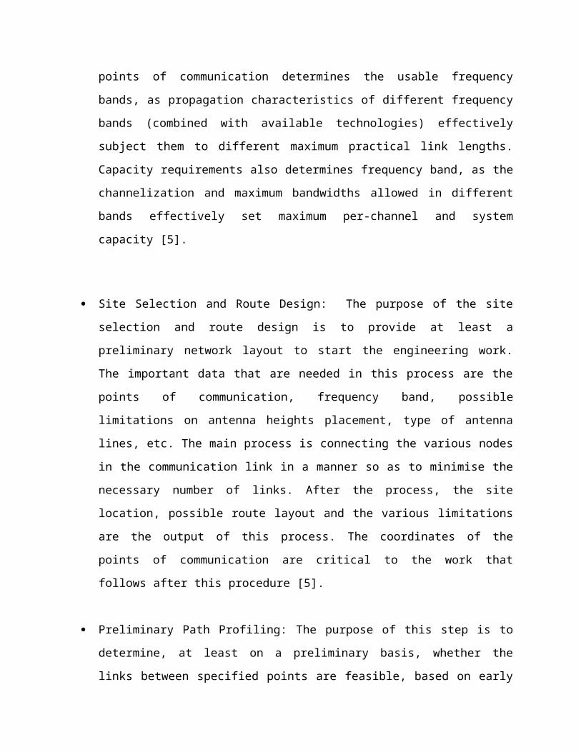
Fig 3.7 Pictures taken during the site survey.

3.8.4 THE VISIT TO ALL SITES

Microwave Radio surveys are carried out for planning of the microwave line of sight links

between point to point or point to multipoint due to the fact that there is no clear line of sight

between Banda Ahenkro and Bui Citya. This was noted when planning for the links using the

Topo-map and Microwave Planning Tool Kit, Aircom-Connet 7.0.

The entire coverage area of the network was critically surveyed using field maps. The study

involves topographical features of the area such as road networks, major organizations in the area

and various possibilities for the establishment of microwave routes and line-of-sight conditions

for all routes. The objective of microwave link radio survey is to;

Select the site for radio equipment and tower location.

Select operational frequency band

Development of path profiles to determine the height of the radio tower.

Analyzing the reflections, refraction and diffraction of the signals.

Calculation of the path loss.

Sites for antenna installation were selected to ensure best line-of sight, easy accessibility and

minimum cost of installation [13].

3.8.5 THE PATH PROFILE FOR THE SELECTED COMMUNITIES

The path profile is the graphical representation of the path travelled by the radio waves between

the two ends of a link. The path profile determines the locations and heights of the antenna at each

end of the link and it ensures that the link is free of obstructions such as hills and not subjected to

propagation losses from radio phenomena such as multipath reflections. Radio LOS requires more

clearance to accommodate the characteristics of microwave signals [19][1].

Using detailed map of the coverage of the network, path profile for all microwave hops in the

network was plotted.

The microwave path profiles for microwave last mile connectivity between to Bui Dam is given

below

Banda Ahenkro Distance/Km (18.05) Bui Dam

Fig 3.8 The Path Profile From Banda Ahenkro To Bui Dam

From the diagram, the property height from ground is 266m above sea level on the tower at

Banda Ahenkro and 250m above sea level at the tower at Bui Dam which is a 45m tower with the

microwave radio height at 45m and 75m at Banda ahenkro which is an 80m tower.

Table 3.2 Coordinates of the selected Communities

3.8.6 THE FRESNEL ZONE CALCULATION

An EM wave does not travel in straight line but spreads out as it propagates. The individual

waves do not also travel at the same velocity. Augustine Fresnel, determined the propagation of a

radio wave as a three dimensional elliptical path between the transmitter and the receiver. Fresnel

divided the path into several zones based on the phase and speed of the propagating waves. The

size of the Fresnel zone varies based on the frequency of the radio signal and the length of the

path. As frequency decrease, the size of the Fresnel zone increase. A Fresnel zone is greatest at

the midpoint of the path. Therefore the midpoint requires most clearance than any point in the

path [4][2].

Name Of Town Longitude /W Latitude/N Site Elevation/m

Bui Citya 002.414598 07.570300 320

Bui City 002.478456 07.35960 360

Fresnel zone

First Fresnel’s zone

Banda Ahenkro Distance/Km Bui Dam

Fig 3.11Fresnel Zone Determination

The first Fresnel zone is given by the formula;

R1=

Where R1 is the radius of the first Fresnel zone,

D1 is the distance from Station A to the point of the higher altitude (obstacle)

D2 is the distance from obstacle to Station B

D is distance between sites (distance between transmitter and receiver)

From Banda Ahenkro to Bui Dam which is 18.05Km apart, the distance from the tower at Banda

Ahenkro to the point of higher altitude which is a hilly area along the road is 2Km, this implies

that the first Fresnel zone is given as;

D1=2.0km / D2 =16.05km

A

B

Then the first Fresnel zone for the link between Banda Ahenkro and Bui City which is separated

by a distance of 18.05 Km and the point of highest altitude which is bunch of trees located in a

thick forest along the path is 2Km from Banda Ahenkro, Hence the first Fresnel zone is given as;

D1=2 Km, D2=16.05Km D=18.05Km

R2=

3.7.7 CALCULATING THE FREE SPACE LOSS (FSL)

Before determining whether a link will be feasible, the FSL should be calculated. The Free Space

Loss is the expected attenuation of a signal as it travels away from the transmitting device. As the

area covered by a spreading signal increases, the power density decreases, this weakens the radio

signal [4] [21]

Mathematically, FSL =32.44 20 log F+ 20 log D

FSL = 92.45 + 20log F+20 log D

Where; F= frequency in MHz/GHz, D= distance in Km.

Although the free space loss equation given above seems to indicate that the loss is frequency

dependent. The attenuation provided by the distance travelled in space is not dependent upon the

frequency. This is constant. The reason for the frequency dependence is that the equation contains

two effects:

The first results from the spreading out of the energy as the sphere over which the energy

is spread increases in area. This is described by the inverse square law.

The second effect results from the antenna aperture change. This affects the way in which

any antenna can pick up signals and this term is frequency dependent [4] [19].

FSL = 92.45 +20log (8) + 20log (18.05),

FSL1 = 139.3 dB,

Hence the FSL between Banda Ahenkro to Bui City is 3dB. and. This implies that from Banda

Ahenkro to Bui City which is 18.05Km apart, the path loss is 139.3dB, hence the output power

selected should be greater than these values.

3.9 THE ANTENNA CONSIDERATION FOR THE PROJECT

The purpose of a transmitting antenna is to radiate electromagnetic wave into “free space”. The power of this is supplied by a “feeder” which is often a length of transmission cable and /or wave guide having well defined characteristic impedance(s), One regard on antenna as a kind of ‘transducer’ to convert the generated electrical energy into radiating energy.

3.9.1 SPACE DIVERSITY ANTENNA

A space diversity antenna is physically two antennas that are space approx. 10m apart and

performs diversity operation. In diversity operation, the radio receives signals on both antennas

but responds on the antenna with the strongest received signal. Diversity operation helps improve

system performance when signal are being reflected and also different paths to the antenna.

Diversity antennas are available in 2.2dBi and 5.3dBi gain ratings [19] [21].

When selecting an antenna, the following needs to be considered.

Lighting protection

directionality required

gain required and cost of energy

Corrosion (Salty Condition )

Proximity to other radio services.

As general guide the following needs to be considered when installing an antenna [19] [21].

Polarization (vertical or Horizontal )

Clearance of near obstructions

Condensation drainage for antenna

Lighting avoidance

Weather proofing connections

Cable bending radius

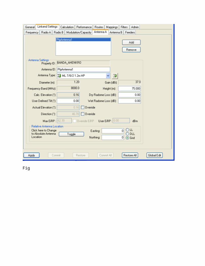
Fig 3.12 A Picture Showing an Existing Hiperion PDH antenna [20]

Fig

Fig

From the diagram, a point to point antenna will be used at both ends of the microwwave radio link. The maximum effective isotropic radiated power transmitted at both ends which is dependant on Frequency of band selected and diameter of the microwave antenna is 62.30 dBm. The selected antenna diameter is 1.20m at the 8GHz frequency.

3.9.3 THE ANTENNA HEIGHT DETERMINATION

In link consideration, if the best type of antenna are implemented in a radio network and there is

no clear line – of - sight for radio wave propagation, the link will not be established, Thus

appropriate antenna and tower heights would have to be estimated to ensure connectivity between

two sites.

According to the international Telecommunication union – Radio sector (ITU – R)

recommendation 530 – 4, appropriate design of terrestrial line – of – sight microwave systems

requires that systems be designed with Clearance above terrain features [16].

The ITU – R suggests the following rules for common use concerning required conditions about

clearance.

hc ≥ ho at k = 4/3 (temperate zone)

hc ≥0.3 ho at k = 2/3

hc ≥ 0.577 ho at k = 0.7 (only for freq of 7GHz and up)

Where;

ho is the 1st Fresnel Zone radius

hc is the clearance

Height asl/m

hl a =75m

h1 =341mh1g = 266m

d1 =2km

D =18.05km

h2g =250m

h2a

hc

hs=280m256m

d2 = 16.05km

24m

Banda Ahenkro Distance/Km Bui City

Fig 3.13 A Detailed Drawing Showing the Path between Banda Ahenkro and Bui City

Where;

d1 = the distance from Banda Ahenkro to the point of the higher altitude

d2 = the distance from point of higher altitude to Bui City

D = the distance between the two sites under consideration ie Banda Ahenkro to Bui City

h1a = the Banda Ahenkro antenna height above the ground

h1g = the ground height above sea level from Station A tower location

h1 = the Station A antenna height above sea level hla+h1g

h2a = the Station B antenna height above of the ground

h2g = the ground height above sea level for the Station B tower location

h2 = the Station B antenna height above sea level = h2a + h2g

hs = the height of the highest obstacle above sea level

hk = the height below sea level at the position of the level highest obstacle in relation to the

effective earth radius.

Where;

k = the earth curvature constant

a = the radius of the earth.

3.9.4 THE REQUIRED CLEARANCE

Clearance (hc) is the distance between the optical line of sight and the nearest obstacle. A clear

line of sight exists when no physical objects exist when viewing one antenna from the other [19].

It is calculated as shown below

Therefore the antenna height can be found from

By Calculation

, but, h2=h2a +h2g

Hence, h2a= 413.07 – 360=53.07m.

A software Applet program was use to calculate the antenna height and hence, the antenna height

and the required clearance were found.

h1 = 90m+320mh1 = 410m

hc = 41.95m

= 0.01027km = 10.27m for hc ho.

hk= 10.27m hs=330 +30m hs= 360m

By using an antenna height calculation tool in the Pathloss4.0, the antenna height at Bui City was

which agrees with the calculations,

h2 =413.07m ho =15.421m h2a=413.07m-360m h2a= 54m.

The required clearance (hc) was also found to be 41.95m which is greater than the 1stFresnel Zone

radius (ho) which is 15.421m. This implies that the calculated antenna heights will have a feasible

line of sight

3.10 RADIO EQUIPMENTS SELECTION

A typical microwave radio transceiver consists of an indoor mounted base band shelf, an indoor

or outdoor mounted radio frequency (RF) transceiver and a parabolic antenna. Each terminal

transmits and receives information to and from the opposite terminal simultaneously providing

full duplex operation. The base band shelf provides the interfaces to other terminating equipment

such as switches, routers, BTS, etc. If the RF transceiver, is an outdoor unit it is mounted directly

behind the parabolic antenna separated by a short run of flexible waveguide.

Careful analyses were made into some radio equipment to ascertain their effectiveness if selected

for this project and the Hiperion SDH link Radio was selected.

Hiperion Digital Microwave Systems allows transmission links to be established rapidly and

easily to meet a variety of transmission needs, delivering cost savings and enabling rapid network

rollout, Hiperion SDH radio system is a full-featured 155Mbit/s transmission solution, covers the

full band of frequencies from 6 GHz to 23 GHz, and uses ASIC technology to achieve a high

level of integration to provide cost, performance, and reliability that is unmatchable in the

industry [20].

3.10.1 TECHNICAL SPECIFICATIONS OF THE HIPERION SDH RADIO SYSTEM

[A] The key features in the Hiperion SDH link radio system are as follows [20];

Standard compliant system for 6-23GHz with 155Mbit/s capacity.

Adaptive Transmit Power Control (ATPC) and high receiver sensitivity for maximum link

reliability and stability

STM-1 interface available as either electrical or optical

Hot standby Tx protection switching with hitless Rx protection switching

Local management to facilitate commissioning.

Equipment configuration stored onto flash memory

NMS with integral routing and management of ODUs and remote IDUs

Built-in testing functions to facilitate commissioning and troubleshooting

Wide operating range on power supply

Compact and light weight for easy installation and reliable performance

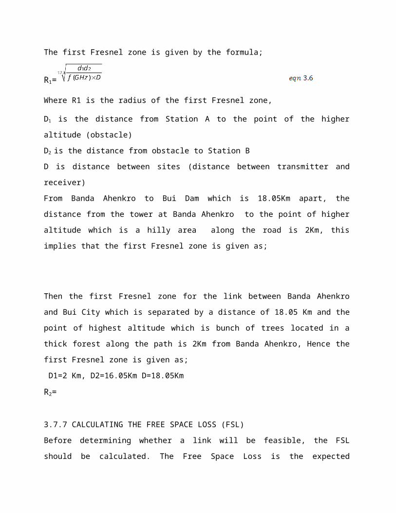
Fig 3.15

A Picture Of The Hiperion PDH Link Radio Equipment [20]

[B] ELECTRICAL AND MECHANICAL SPECIFICATIONS AT 6GHz, 7GHz AND 8GHz

RESPECTIVELY OF THE HIPERION SDH LINK SYSTEM [20].

  6 GHz 7 GHz 8 GHz

Frequency Range GHz 5.925-7. 110 7.10-7.90 7.90-8.50

Electrical characteristics

MHz

ITU-R RF Tx/Rx Spacing 252.04 (Lower)

350 (Upper) 154 or 161

119, 126 or 311.32

RF Channel Bandwidth MHz 28

Tx power at Antenna port

(±2dB tolerance)

dBm 21

Tx Power Control Range

(1 dB step)

dBm 0 to +21

Receive Sensitivity @

BER = 1x10-6

(Guaranteed: +2dB)

dBm -68

Supported RF

Configurations

1+0, 1+1

Radio Protection   Hot standby/ Space diversity / Frequency diversity

Power characteristics

Noise Figure

dB

= 5.5

Power Supply VDC -20 to -60V

Power Consumption (per

hop)

1+0 W = 105

1+1 = 210

IF Connection on ODU   N-type connector, Belden 9913/RG-8, up to 300m

RSSI Connection on

ODU

BNC

Mechanical characteristics

Dimensions (H x W x D) mm 279 x 240 x92

Weight kg 4.2

Operating Temperature ºC -50 to +55

Operational Altitude

Above Mean Sea Level

m 4500

(max)

Operating Humidity % =95

Table 3.3 Radio Equipment Specification

CHAPTER FOUR- THE NETWORK DESIGN ANALYSIS

4.1 THE RECEIVED POWER LEVEL

NO TOWN D(km) PL (dB) Si (dBm)

1 Banda Ahenkro- Bui City 8.5km -65.50

2 Banda Ahenkro- Bui City 12.8km

3

Banda Ahenkro- Bui City 16km

4 Banda Ahenkro- Bui City 18km

Table 4.0 Received power levels at various locations

Thus, all the radio equipment having sensitivity within the measured power levels should be

possible to receive the signal at these various locations. Therefore, the Hiperion PDH radio

system that has been selected for the project will be able to receive the signals been transmitted

because it has a receiver sensitivity at BER 1 -6 to be -68 dBm.

4.2 THE CALCUALTION OF THE LINK BUDGET

Receiver sensitivity is the minimum signal power level required at the input receiver for

certain performance.

The antenna Effective Isotropic Radiated Power (EIRP) is the transmitted power which is equal to

the transmitted output power minus cable loss plus transmitting antenna gain [4].

Mathematically,

EIRP = Pout – Ct + Gt eqn 4.0

Si = EIRP –FSL+ Gr - Cr eqn 4.1

Where; Ct = transmitter cable loss Cr = receiver cable loss Si = received power at the receiver

input.

The received signal power should be above the sensitivity threshold. To determine if a link will be

feasible, the calculated received signal level is compared with the receiver sensitivity threshold,

the link is theoretically feasible if , which means that the signal will be strong enough to

successfully interpreted by the receiver [4]?

4.3 THE LINK BUDGET FOR BANDA AHENKRO TO BUI CITYA

Link Details

Link IDBanda_Ahenkro - Bui_Dam

1st Name2nd NameLink Type Default MicrowaveDuplex Method FDDPacket Size(bytes) 100Packet Type IPv4Synchronisation N/ADelay(ms) N/AActual Latency(ms) N/ALink Modified Date 2012-11-22 11:03:25LOS Status ClearMain Band 8G_14M_119 DSMain Band Duplex Method FDDMain Channel F3Main Polarisation VerticalCalculation Method ITU-R P. 530-12

dN1 (N-unit/km) -87.935566Geoclimatic factor K 0.00004923Terrain Type ForestITU Climate Region/Rate ACurrent RainModel ITU_RAIN_MODEL% Time Rainfall 0.0100

Capacity BANDA_AHENKRO Bui CityMain Ethernet Capacity(Kbps) 56000 56000Main Total Capacity(Kbps) 56000 56000Main Control Overhead(Kbps) 21280 21280Capacity Status Sufficient SufficientMain Available Capacity(Kbps) 34720 34720Main Centre Frequency (GHz) 8.321000 8.440000Main Bandwidth (MHz) 14.00000 14.00000Main Frequency Designation Low HighProperty ID BANDA_AHENKRO BUI_DAM_NEWProperty Latitude 08°09'46.01"N 08°16'28.30"NProperty Longitude 002°21'28.01"W 002°14'18.06"WProperty Height (m) 266.00 250.00Mast Name 80 m Tower 45 m TowerMast Type Ground GroundMast Height 80.00 45.00Main Antenna Type ML 7/8/2 1.2m HP ML 7/8/2 1.2m HPMain Antenna Size (m) 1.20 1.20Main Antenna Height (m) 75.00 40.00Main Antenna Ground Height (m) 266.00 250.00Main Antenna Direction (°) 46.70 226.70Main Actual Elevation (°) 0.16 -0.16Main Antenna Gain (dB) 37.0 37.0Main EiRP (dB) 62.30 62.30Main Feeder Type ML 7/8 0.9m Asy ML 7/8 0.9m AsyMain Feeder Length (m) 160.00 90.00Main Feeder Loss (dB) 1.70 1.70Main Radio Type MLT 8/ 2X 045/16S S MLT 8/ 2X 045/16S SMain Min Tx Power (dBm) 0.00 0.00Main Max Tx Power (dBm) 27.00 27.00Main Operating Mode HotSB HotSBMain Threshold -81.00 dBm @ BER 10^-6 -81.00 dBm @ BER 10^-6 Main ATPC Value (dB) 37.00 37.00Main Modulation Type 16QAM 16QAMMax Achievable Throughput(Mbps) 34.7200 34.7200

Main Required Availability(%) 99.9900 99.9900Main High Priority Availability(%) 99.9900 99.9900

Performance Banda AhenkroBui City

Total Antenna Gain (dBi) 74.0000

Total Anten. Loss (dB) 0.0000 0.0000Total Dry Radome Loss (dB) 0.0000Total Feeder Loss (dB) 3.4000Total Branching Loss (dB) 0.0000 0.0000Total Misc Loss (dB) 0.0000 0.0000Freespace Loss (dB) 136.1049 135.9816Atmospheric Absorption (dB) 0.2194 0.2165Obstruction Loss (dB) 0.0000 0.0000Total Loss (dB) 139.7243 139.5981

Rx Level (dBm) -38.7243 -38.5981Linkend Antenna Gain (dBm) 37.0000 37.0000Threshold Value (dBm) -81.0000 -81.0000Composite Fade Margin (dBm) 42.1610 42.2838Flat Fade Margin (dB) 42.2757 42.4019Flat Fade Margin After Interference (dB) 42.2757 42.4019Req. FM Against Rain (dBm) 0.9028Dispersive Fade Margin (dB) 58.0000 58.0000Flat Outage (PnS) (%) 0.0000088 0.0000085Selective Outage (Ps) (%) 0.0000018 0.0000018Annual Unavailability (%) 0.0025350 0.0025350Annual Availability (%) 99.9974650 99.9974650Annual Availability (s/yr) 31535200.55 31535200.55Link PER 0.000 0.000

Optimum Packet Size(bytes) 1518 1518Optimum Available Capacity(Kbps) 54598.156 54598.156Objective Calculation Method ITU-T Y 1541 ITU-T Y 1541Link Grade AccessLink ClassHop Length (km) 18.047Error Performance 7.50SESR Objective 1.50e-4

SES/month 388.80000000

Table 4.1 The link budget for Banda Ahenkro To Bui City.

It could be verified from the above that the received signal levels are all greater than the receiver

sensitivity and hence the receiver will be able to intercept the signals and correctly decode

without interference and that our network will be feasible.

4.4 PATH RELIABILITY AND AVAILABITY ANALYSIS

Usually, microwave links are designed to meet a specific reliability factor. Reliability is expressed

as a percentage. It represents the percentage of time the link is expected to operate without an

outage caused by propagation conditions. The Bell standard for short-haul propagation reliability

is 99.995% (minimum), while requirements for high-capacity, long-haul may be 99.9999% [21].

"Unavailability" or the probability of an outage because of propagation conditions is often

referred to and, if expressed in percentage, the value is determined by subtracting the availability

(expressed as a percentage) from 100 [21].

Availability and unavailability are referenced to a year. For the path between Banda Ahenkro to

Bui City where the availability is 99.9974650, then, the unavailability is 0.0025350, thus, the

outage per year is given as;

[365.25(days/yr)* 24(hr/day) * 60 (min/hr) * (0.001/100)]= 31535200.55 minutes of

unavailability (outage) per year [21].

4.5 THE NETWORK DESIGN AND COST ANALYSIS

The objective of the network design is to link up the some communities in the Jaman North

district of Brong Ahafo region to the Vodafone GH network from Banda Ahenkro which is the

nearest Vodafone GH Exchange where the microwave network can be reach. With the application

of fixed line and GSM for that matter coupled with other technological advantages, workers and

citizens can have access to telephone services, internet, fax, and not forgetting the opportunity to

access Vodafone GH mobile network in the Area as well as other ICT facilities.

4.7 COST ANALYSIS

Capital CostsCost

TX

BX

M D

B T S

4.6 PROPOSED NETWORK DESIGN FOR THE JAMAN NORTH

LinkID Installation LinkTermEquip RadioEquipmentCost Antenna

Banda_Ahenkro - Bui_Dam 20000 1500.00 5000 4000

Annual Operating CostsCost

LinkID Maintenance Rental TotalBanda_Ahenkro - Bui_Dam 10000 3000 13000

From the table, the capital cost of mainting a site a Bui City will cost USD ,.