Chapter Six Electrostatic Energy

Electromagnetic Theory 2018-2019 Prof. dr. Ali Hadi Hassan Al-Batat 1-15

1

Chapter Six

Electrostatic Energy In general, the energy of a system of charges, just like that of any other mechanical

system, may be divided into its potential and kinetic contributions. Under static

conditions, however, the entire energy of the charge system exists as potential

energy, and we are particularly concerned with that potential energy which arises

from electrical interaction of the charges, the so-called electrostatic energy.

In chapter four, it was shown that the electrostatic energy of a point charge is closely

related to the electrostatic potential U at the position of the point charge. In fact, if q

is the magnitude of a particular point charge, then the work done on the charge in

moving it from position A to position B is

𝑊𝑜𝑟𝑘 = ∫ �⃗�𝒎. 𝑑𝑙 =𝐵

𝐴− 𝑞 ∫ �⃗⃗�. 𝑑𝑙 = 𝑞 ∫ 𝒈𝒓𝒂𝒅𝑈. 𝑑𝑙 = 𝑞(𝑈𝐵 − 𝑈𝐴)

𝐵

𝐴

𝐵

𝐴 (1)

Here, the mathematical force, �⃗�𝒎 has been chosen so as to balance exactly the

electric force 𝑞�⃗⃗� at each point along the path. Under these conditions the charged

particle does not accelerate, and equation (1) represents the change in electrostatic

energy of the charge over the path interval 𝐴 → 𝐵.

In fact, the e1ectrostatic energy of an arbitrary charge distribution may be calculated

as the work required to assemble this distribution of charge without imparting to it

other forms of energy.

1. Potential Energy of a Group of Point Charges

By the electrostatic energy of a group of m point charges, we mean the potential

energy of the system relative to the state in which all point charges are infinitely

separated from one another. This energy can be obtained by calculating the work

done to assemble the charges. The first charge 𝑞1 may be placed in position without

the expenditure of energy;

To place the second charge, 𝑞2, requires,

∆𝑊2 =𝑞1𝑞2

4𝜋𝜀0𝑟12 (2)

Where 𝑟12 = ⃒𝑟1 − 𝑟2 ⃒

For the third charge, 𝑞3


2

∆𝑊3 = 𝑞3[𝑞1

4𝜋𝜀0𝑟13+

𝑞2

4𝜋𝜀0𝑟23] (3)

The work required to bring in the fourth charge, fifth charge, etc, written in similar

fashion.

It will be convenient to symmetrize each of these terms by repeating each entry with

indices reversed and having the result. In other words, we rewrite equation (2) as

∆𝑊2 =1

8𝜋𝜀0[

𝑞1𝑞2+𝑞2𝑞1

𝑟12] (4)

The succeeding terms are similarly rewritten

∆𝑊3 =1

8𝜋𝜀0[


𝑟13+


𝑟23] (5)

∆𝑊4 =1

8𝜋𝜀0[


𝑟14+


𝑟24+


𝑟34] (6)

Finally, to put the nth charge into place,

∆𝑊𝑛 =1

8𝜋𝜀0[

𝑞1𝑞𝑛+𝑞𝑛𝑞1

𝑟1𝑛+


𝑟2𝑛+


𝑟3𝑛+ ⋯ … … . +

𝑞𝑛−1𝑞𝑛+𝑞𝑛𝑞𝑛−1

𝑟𝑛−1,𝑛] (7)

We add the terms to obtain the work to assemble all the charges,

𝑊 = ∆𝑊2 + ∆𝑊3 + ∆𝑊4 + ⋯ … + ∆𝑊𝑛 (8)

=1

8𝜋𝜀0[𝑞1 (

𝑞2

𝑟12+

𝑞3

𝑟13+

𝑞4

𝑟14+ ⋯ … … +

𝑞𝑛

𝑟1,𝑛) + 𝑞2 (

𝑞1

𝑟21+

𝑞3

𝑟23+

𝑞4

𝑟24+ ⋯ … +

𝑞𝑛

𝑟2,𝑛) +𝑞3 (

𝑞1

𝑟31+

𝑞2

𝑟32+

𝑞4

𝑟34+ ⋯ … … +

𝑞𝑛

𝑟3,𝑛) + ⋯ +𝑞𝑛−1 (

𝑞1

𝑟𝑛−1,1+

𝑞2

𝑟𝑛−1,2+

𝑞4

𝑟𝑛−1,4+

⋯ … … +𝑞𝑛

𝑟𝑛−1,𝑛)] (9)

=1

8𝜋𝜀0∑ 𝑞𝑗 ∑

𝑞𝑘

𝑟𝑗𝑘=

1

8𝜋𝜀0∑ ∑

𝑞𝑗𝑞𝑘

𝑟𝑗𝑘

𝑛𝑘=1𝑘≠𝑗

𝑛𝑗=1


𝑛−1𝑗=1 (10)


3

where in the last step we have increased the upper limit of the 𝑗 summation by one

which adds nothing as the (n,n) term is eliminated from the sum by the 𝑘 ≠ 𝑗

requirement. It is useful to rewrite W as

𝑊 =1

2∑ ∑

𝑞𝑘

4𝜋𝜀0


𝑛𝑗=1

𝑞𝑗

𝑟𝑘𝑗=

1

2∑ 𝑞𝑗 ∑

1

4𝜋𝜀0


𝑛𝑗=1

𝑞𝑘

𝑟𝑘𝑗 (11)

Where 𝑊 is the total electrostatic energy of the assembled n-charge system which

is the sum of the ΔW’s.

Equation (11) may be written in a somewhat different way by noting that the final

value of the potential U at the jth point charge is

𝑈𝑗 = ∑1

4𝜋𝜀0


𝑞𝑘

𝑟𝑘𝑗 (12)

Thus, the electrostatic of the system is

𝑊 =1

2∑ 𝑞𝑗𝑈𝑗

𝑛𝑗=1 (13)

2. Electrostatic Energy of a Charge Distribution

Suppose we assemble the charge distribution by bringing in charge increments 𝛿𝑞

from a reference potential 𝑈𝐴 = 0. If the charge distribution is partly assembled and

the potential at a particular point in the system is 𝑈′(𝑥, 𝑦, 𝑧), then, from equation (1),

the work required to place 𝛿𝑞 at this point is

𝛿𝑊 = 𝑈′(𝑥, 𝑦, 𝑧)𝛿𝑞 (14)

The charge increment 𝛿𝑞 may be added to a volume element located at (𝑥, 𝑦, 𝑧),

such that 𝛿𝑞 = 𝛿𝜌∆𝑣 or 𝛿𝑞 may be added to a surface element at the point in

question, whereby 𝛿𝑞 = 𝛿𝜎∆𝑎. The total electrostatic energy of the assembled

charge distribution is obtained by summing contributions of the form (14).

𝑊 =1

2∫ 𝜌𝑈 𝑑𝑣 +

1

2∫ 𝜎𝑈 𝑑𝑎

𝑆𝑣 (15)

It was stipulated that conductors are present in the system. The last integral involve,

in part, integrations over the surface of these conductors; since a conductor is an

equipotential region, each of these integrations may be done:


4

1

2∫ 𝜎𝑈 𝑑𝑎 =

1

2𝑄𝑗𝑈𝑗𝑐𝑜𝑛𝑑𝑢𝑐𝑡𝑜𝑟 𝑗

(16)

Where 𝑄𝑗 is the charge on the jth conductor. Hence equation (15) becomes

𝑊 =1

2∫ 𝜌𝑈 𝑑𝑣 +

1

2∫ 𝜎𝑈 𝑑𝑎 +

1

2𝑆′𝑣∑ 𝑄𝑗𝑈𝑗𝑗 (17)

where the last summation is over all conductors, and the surface integral

is restricted to nonconducting surfaces.

Since, in many problems of practical interest all of the free charge resides on the

surfaces of conductors. In these circumstances equation (17) reduces to

𝑊 =1

2∑ 𝑄𝑗𝑈𝑗𝑗 (18)

3. Energy density of an electrostatic field

Consider an arbitrary distribution of free charge characterized by the densities 𝜌 and

𝜎. The densities 𝜌 and 𝜎 are related to the electric displacement;

𝜌 = div D⃗⃗⃗ throughout the dielectric regions, and 𝜎 = �⃗⃗⃗�. �̂� on the conductor surfaces.

Hence, equation (15) becomes

𝑊 =1

2∫ 𝑈 div D⃗⃗⃗ 𝑑𝑣 +

1

2∫ 𝑈 �⃗⃗⃗�. �̂� 𝑑𝑎

𝑆𝑣 (19)

The volume integral here refers to the region where div D⃗⃗⃗ is different from zero, and

this is the region external to the conductors. The surface integral is over the

conductors.

The integrand in the first integral of equation (19) may be transformed by means of

the following vector identity; 𝑑𝑖𝑣 𝜑�⃗� = 𝜑 𝑑𝑖𝑣 �⃗� + �⃗�. ∇⃗⃗⃗𝜑, into

𝑈 div D⃗⃗⃗ = div UD⃗⃗⃗ − �⃗⃗⃗�. ∇⃗⃗⃗𝑈

Substituting in equation (19), we obtain

𝑊 =1

2∫ div UD⃗⃗⃗ 𝑑𝑣 −

1

2∫ �⃗⃗⃗�. ∇⃗⃗⃗𝑈 𝑑𝑣 +

𝑣

1

2∫ 𝑈 �⃗⃗⃗�. �̂� 𝑑𝑎

𝑆𝑣


5

By using the divergence theorem, the first term in last equation can be transformed

to surface integral, thus the last equation becomes

𝑊 =1

2∫ UD⃗⃗⃗. �̂�′ 𝑑𝑣

𝑆+𝑆′+

1

2∫ �⃗⃗⃗�. E⃗⃗⃗ 𝑑𝑣 +

𝑣

1

2∫ 𝑈 �⃗⃗⃗�. �̂� 𝑑𝑎

𝑆 (20)

This equation may be simplified substantially. The surface S + S' over which the

first integral of (20) is to be evaluated is the entire surface bounding the volume V.

It consists, in part, of S (the surfaces of all conductors in the system), and also of S'

(a surface which bounds our system from the outside, and, which may choose to

locate at infinity). In both cases the normal n' is directed out of the volun1e V. In the

last integral the normal n is directed out of the conductor, hence into V. Thus, the

two surface integrals over S cancel each other. It remains to show that the integral

over S' vanishes.

If the charge distribution, which is arbitrary but bounded, bears a net charge, then at

large distances from the charge system the potential falls off inversely as the

distance, i.e., as r-1. D falls off as r-2. The area of a closed surface which passes

through a point at distance r is proportional to r2. Hence the value of the integral over

S' which bounds our system at distance r is proportional to r-1 and S' is moved out

to infinity, its contribution vanishes.

Thus, for the electrostatic energy, we have

𝑊 =1

2∫ �⃗⃗⃗�. E⃗⃗⃗ 𝑑𝑣

𝑣 (21)

Hence, the energy density in an electrostatic field is

𝜔 =1

2�⃗⃗⃗�. E⃗⃗⃗ (22a)

Since equation (21), was derived on the basis o:f linear dielectrics, each dielectric is

characterized by a constant permittivity 휀. Furthermore, the discussion in preceding

chapters has been limited to isotropic dielectrics. Thus equation (22a) is equivalent

to

𝜔 =1

2휀𝐸2 (23)


6

Problem.1: If the electric field in a vacuum is defined by �⃗⃗� = 2𝑟 sin 𝜃�̂�𝑟 − 𝑟 cos 𝜃 �̂�𝜃 .

Find the energy in the region 0 ≤ 𝑟 ≤ 5 and 0 ≤ 𝜃 ≤ 𝜋/3.

Solution: by using 𝑊 =𝜀0

2∫ 𝐸2𝑑𝑣, we obtain

𝑊 =𝜀0

2∫ ∫ ∫ [4𝑟2 sin2 𝜃 + 𝑟2 cos2 𝜃]𝑟2𝑑𝑟 sin 𝜃𝑑𝜃𝑑𝜑 =

9

554𝜋휀0

5

0

𝜋/3

0

2𝜋

0

H.W: If the electrostatic potential in a vacuum is defined by 𝑈 = 𝑥 − 𝑦 + 𝑥𝑦 + 2𝑧. Find

the electric field at the point (1,2,3) and the energy stored in a cube of length a centered at

the origin.

Problem.2: A charge distribution with spherical symmetry has density

𝜌 = {𝜌0 0≤𝑟≤𝑅

0 𝑟 > 𝑅

Determine U everywhere and the energy stored in region r < R.

Solution:

The �⃗⃗⃗� field has already been found in chapter two using Gauss's law.

a) For 𝑟 ≥ 𝑅 , �⃗⃗� =𝜌0𝑅3

3𝜀0𝑟2�̂�𝑟

Once �⃗⃗� is known, U is determined as

𝑈 = − ∫ �⃗⃗�. 𝑑𝑙 = −𝜌0𝑅3

3𝜀0∫

1

𝑟2𝑑𝑟

=𝜌0𝑅3

3𝜀0𝑟+ 𝐶1

Since, 𝑈(𝑟 = ∞) = 0, 𝐶1 = 0

b) For 𝑟 ≤ 𝑅, �⃗⃗� =𝜌0𝑟

3𝜀0�̂�𝑟

hence,

𝑈 = − ∫ �⃗⃗�. 𝑑𝑙 = −𝜌0

3𝜀0∫ 𝑟𝑑𝑟

= −𝜌0𝑟2

6𝜀0+ 𝐶2

To determine the constant 𝐶2 equating the potential at r=R

From part (a) , 𝑈(𝑟 = 𝑅) =𝜌0𝑅2

3𝜀0, hence

𝜌0𝑅2

3𝜀0= −

𝜌0𝑅2

6𝜀0+ 𝐶2 , thus, 𝐶2 =

𝜌0𝑅2

2𝜀0

and


7

𝑈 =𝜌0

6𝜀0(3𝑅2 − 𝑟2)

Thus, from part (a) and (b)

𝑈 = {

𝜌0𝑅3

3𝜀0𝑟 𝑟 ≥ 𝑅

𝜌0

6𝜀0(3𝑅2 − 𝑟2) 𝑟 ≤ 𝑅

(c) The energy stored is given by

𝑊 =1

2∫ �⃗⃗⃗�. E⃗⃗⃗ 𝑑𝑣

𝑣=

1

2휀0 ∫ 𝐸2𝑑𝑣

For 𝑟 ≤ 𝑅 �⃗⃗� =𝜌0𝑟

3𝜀0�̂�𝑟

H.W: Find the energy stored in free space for the region 2𝑚𝑚 < 𝑟 < 3𝑚𝑚, 0 < 𝜃 <

900, 0 < 𝜑 < 900, given the potential field (a) 200

𝑟𝑉, (b)

300 𝑐𝑜𝑠 𝜃

𝑟2𝑉. Ans.: 1.391pJ, 36.7J


8

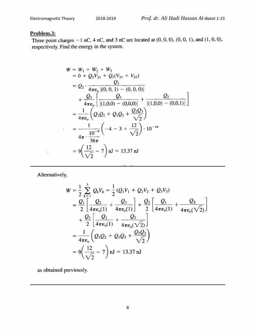
Problem.3:


9

4. Energy of a system of charged conductors. Coefficients of potential It was shown that a linear relationship exists between the potentials and charges on

a set of conductors. In fact, in a system composed of N conductors, the potential of

one of them is given by

𝑈𝑖 = ∑ 𝑝𝑖𝑗𝑄𝑗𝑁𝑗=1 (24)

The derivation of equation (24) was carried out for N conductors in vacuum;

however, it is clear that, this derivation also holds when dielectrics are present in the

system, so long as these dielectrics are both linear and devoid of free charge. The

coefficient 𝑝𝑖𝑗 is the potential of the ith conductor due to a unit charge on conductor

j. These coefficients are usually referred to as coefficients of potential. Combing

equations (18) and (24), we obtain

𝑊 =1

2∑ ∑ 𝑝𝑖𝑗𝑄𝑖𝑄𝑗

𝑁𝑗=1

𝑁𝑖=1 (25)

Thus the energy is a quadratic function of the charges on the various conductors.

A number of general statements can be made about the coefficients 𝑝𝑖𝑗, which are:

1- 𝑝𝑖𝑗 = 𝑝𝑗𝑖

2- all of the 𝑝𝑖𝑗 are positive

3- 𝑝𝑖𝑖 − 𝑝𝑖𝑗 ≥ 0

To prove the first statement we can expresses 𝑊 as 𝑊(𝑄1, … . . , 𝑄𝑁); thus

𝑑𝑊 = (𝜕𝑊

𝜕𝑄1) 𝑑𝑄1 + ⋯ … … . + (

𝜕𝑊

𝜕𝑄𝑁) 𝑑𝑄𝑁

If 𝑑𝑄1 only is changed, then

𝑑𝑊 = (𝜕𝑊

𝜕𝑄1) 𝑑𝑄1 =

1

2∑ (𝑝1𝑗 + 𝑝𝑗1)𝑄𝑗𝑑𝑄1

𝑁𝑗=1 (26)

Bringing in 𝑑𝑄1 from a zero potential reservoir can also be obtained using the

expression 𝑊 = 𝑄𝑈, thus,

𝑑𝑊 = 𝑈1𝑑𝑄1 = ∑ 𝑝1𝑗𝑄𝑗𝑑𝑄1𝑁𝑗=1 (27)


10

The last two equations must be equivalent for all possible values of the 𝑄𝑗, which

implies that

1

2(𝑝1𝑗 + 𝑝𝑗1) = 𝑝1𝑗 , or

𝑝𝑗1 = 𝑝1𝑗 (28)

H.W: Prove the second and third statements.

The usefulness of the coefficients 𝑝𝑖𝑗 may be illustrated by means of a simple

example. Problem: to find the potential of an uncharged spherical conductor in the

presence of a point charge 𝑞 at distance r, where r > R, and R is the radius of the

spherical conductor. The point charge and sphere are taken to be a system of two

conductors, and use is made of the equality 𝑝12 = 𝑝21. If the sphere is charged (Q)

and the ‘’point" uncharged, then the potential of the point" is 𝑄

4𝜋𝜀0𝑟 ; thus

𝑝12 = 𝑝21 =1

4𝜋𝜀0𝑟

Evidently, when the ‘’point" has charge 𝑞 and the sphere is uncharged, the potential

of the latter is 𝑞

4𝜋𝜀0𝑟.

5. Coefficients of capacitance and induction

Equation (24) is a set of N linear equations giving the potentials of the conductors

in terms of their charges. This set of equations may be solved for the 𝑄𝑖 ’𝑠, yielding

𝑄𝑖 = ∑ 𝑐𝑖𝑗𝑈𝑗𝑁𝑗=1 (29)

where 𝑐𝑖𝑗 is called a coefficient of capacitance and 𝑐𝑖𝑗 (𝑖 ≠ 𝑗) is a coefficielt of

induction. The actual inversion of equation (24) expressing each c in terms of the

𝑝𝑖𝑗, is most easily done by using deterlninants.

Properties of the 𝑐𝑖𝑗 follow from those of the 𝑝𝑖𝑗, which are

1- 𝑐𝑖𝑗 = 𝑐𝑗𝑖 2- 𝑐𝑖𝑖 > 0 3- The coefficients of induction are negative or

zero.


11

Equation (29) may be combined with equation (18) to give an alternative expression

for the electrostatic energy of an N-conductor system:

𝑊 =1

2∑ ∑ 𝑐𝑖𝑗𝑈𝑖𝑈𝑗

𝑁𝑗=1

𝑁𝑖=1 (30)

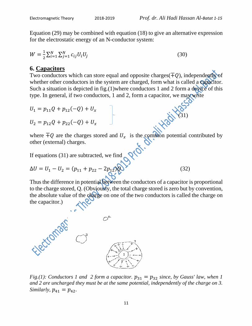
6. Capacitors Two conductors which can store equal and opposite charges(∓𝑄), independently of

whether other conductors in the system are charged, form what is called a capacitor.

Such a situation is depicted in fig.(1)where conductors 1 and 2 form a device of this

type. In general, if two conductors, 1 and 2, form a capacitor, we may write

𝑈1 = 𝑝11𝑄 + 𝑝12(−𝑄) + 𝑈𝑥

(31)

𝑈2 = 𝑝12𝑄 + 𝑝22(−𝑄) + 𝑈𝑥

where ∓𝑄 are the charges stored and 𝑈𝑥 is the common potential contributed by

other (external) charges.

If equations (31) are subtracted, we find

∆𝑈 = 𝑈1 − 𝑈2 = (𝑝11 + 𝑝22 − 2𝑝12)𝑄 (32)

Thus the difference in potential between the conductors of a capacitor is proportional

to the charge stored, Q. (Obviously, the total charge stored is zero but by convention,

the absolute value of the charge on one of the two conductors is called the charge on

the capacitor.)

Fig.(1): Conductors 1 and 2 form a capacitor. 𝑝31 = 𝑝32 since, by Gauss' law, when 1

and 2 are uncharged they must be at the same potential, independently of the charge on 3.

Similarly, 𝑝41 = 𝑝42.


12

Equation (32) may be written

𝑄 = 𝐶∆𝑈 (33)

Where 𝐶 = (𝑝11 + 𝑝22 − 2𝑝12)−1 is called the capacitance of the capacitor.

Evidently C is the charge stored per unit of potential difference; in the mks system

C is measured in coulombs/volt, or farads (1 farad ≡ 1 coulomb/volt).

Using the results of previous sections in this chapter, the energy of a charged

capacitor may be written as

𝑊 =1

2𝐶(∆𝑈)2 =

1

2𝑄∆𝑈 =

1

2

𝑄2

𝐶 (34)

If the two conductors making up the capacitor have simple geometrical shapes, the

capacitance may be obtained analytically. Thus, for example, it is easy to calculate

the capacitance of two parallel plates, two coaxial cylinders, two concentric spheres,

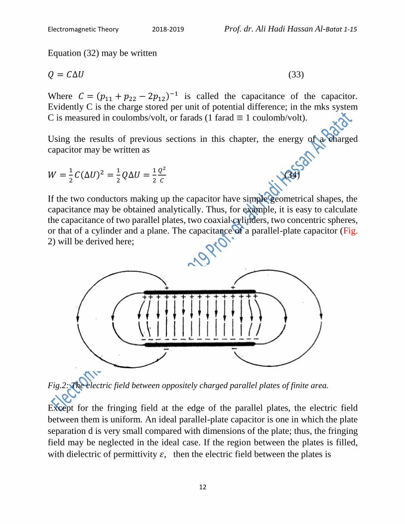
or that of a cylinder and a plane. The capacitance of a parallel-plate capacitor (Fig.

2) will be derived here;

Fig.2: The electric field between oppositely charged parallel plates of finite area.

Except for the fringing field at the edge of the parallel plates, the electric field

between them is uniform. An ideal parallel-plate capacitor is one in which the plate

separation d is very small compared with dimensions of the plate; thus, the fringing

field may be neglected in the ideal case. If the region between the plates is filled,

with dielectric of permittivity 휀, then the electric field between the plates is


13

𝐸 =1

𝜀𝜎 =

𝑄

𝜀𝐴 (35)

where A is the area of one plate. The' potential difference ∆𝑈 = 𝐸𝑑. Therefore,

𝐶 =𝑄

∆𝑈=

𝜀𝐴

𝑑 (36)

is the capacitance of this capacitor.

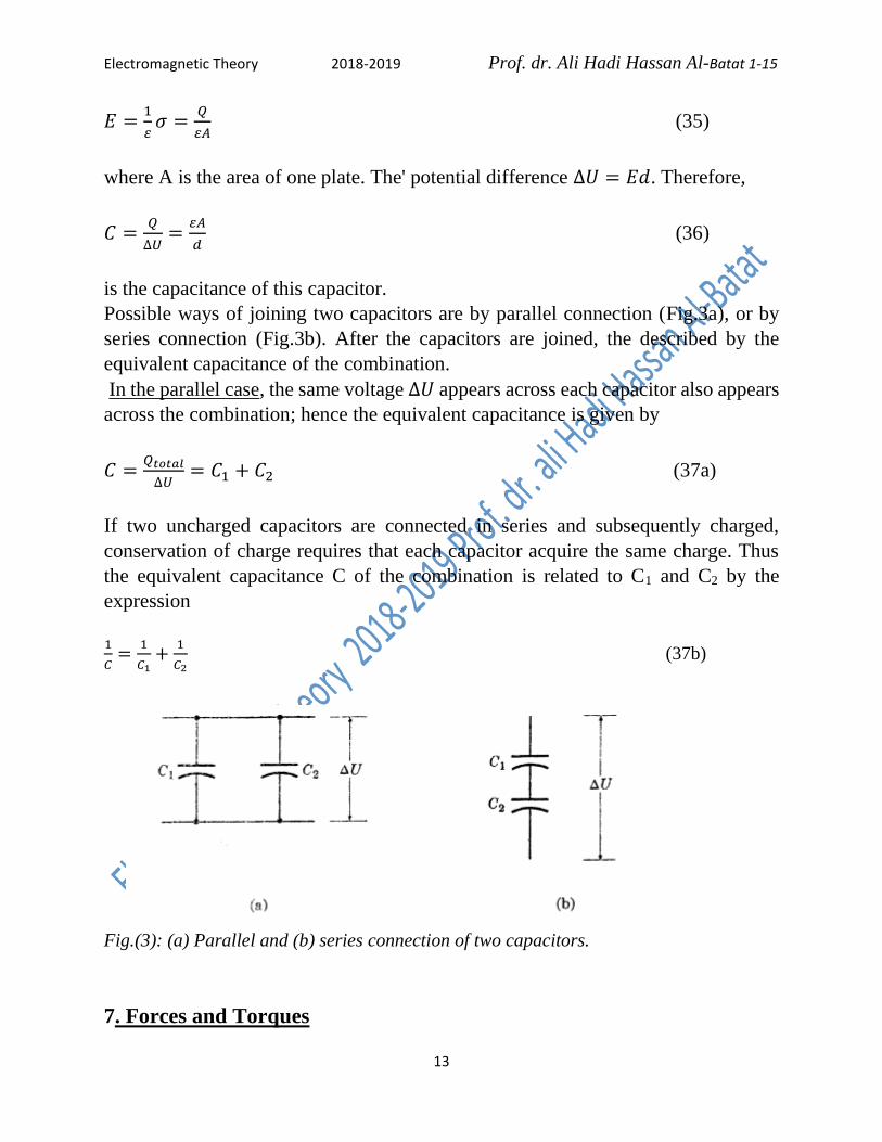
Possible ways of joining two capacitors are by parallel connection (Fig.3a), or by

series connection (Fig.3b). After the capacitors are joined, the described by the

equivalent capacitance of the combination.

In the parallel case, the same voltage ∆𝑈 appears across each capacitor also appears

across the combination; hence the equivalent capacitance is given by

𝐶 =𝑄𝑡𝑜𝑡𝑎𝑙

∆𝑈= 𝐶1 + 𝐶2 (37a)

If two uncharged capacitors are connected in series and subsequently charged,

conservation of charge requires that each capacitor acquire the same charge. Thus

the equivalent capacitance C of the combination is related to C1 and C2 by the

expression

1

𝐶=

1

𝐶1+

1

𝐶2 (37b)

Fig.(3): (a) Parallel and (b) series connection of two capacitors.

7. Forces and Torques


14

In this chapter we have developed a number of alternative procedures for calculating

the electrostatic energy of a charge system. We shall now show how the force on

one of the objects in the charge system may be calculated from a knowledge of this

electrostatic energy. Let us suppose we are dealing with an isolated system

composed of a number of parts (conductors, point charges, dielectrics), and we allow

one of these parts to make a small displacement 𝑑𝑟 under the influence of the

electrical forces acting upon it.

The mechanical work performed by the system in these circumstances is

𝑑𝑊𝑚 = �⃗�. 𝑑𝑟

= 𝐹𝑥𝑑𝑥 + 𝐹𝑦𝑑𝑦 + 𝐹𝑧𝑑𝑧 (38)

Because the system is isolated, this work is done at the expense of the electrostatic

energy W; in other words,

𝑑𝑊 + 𝑑𝑊𝑚 = 0 (39)

Combining equations (38) and (39)

−𝑑𝑊 = 𝐹𝑥𝑑𝑥 + 𝐹𝑦𝑑𝑦 + 𝐹𝑧𝑑𝑧

and 𝐹𝑥 = −𝜕𝑊

𝜕𝑥 (40)

with similar expressions for Fy and Fz.

If the object under consideration is constrained to move in such away that it rotates

about an axis, then equation (38) may be replaced by

𝑑𝑊𝑚 = 𝜏. 𝑑𝜃 (41)

Where 𝜏 is the electrical torque and 𝑑𝜃 is the angular displacement, writing

𝜏 and 𝑑𝜃 in terms of their components (𝜏1, 𝜏2, 𝜏3), (𝑑𝜃1, 𝑑𝜃2, 𝑑𝜃3 ),

and combining equations (39) and (41), we obtain

𝜏1 = −𝜕𝑊

𝜕𝜃1 and similar to 𝜏2 and 𝜏3.


15

The electrostatic energy W of a system of charged conductors has been given earlier,

in equation (13). If, now, some part of the system is displaced while at the same time

the potentials of all conductors remain fixed,

𝑑𝑊 =1

2∑ 𝑈𝑗𝑑𝑄𝑗𝑗 (42)

In general, the energy of the system may be calculated in terms of the electric field

vector from the following equation;

𝑊 =1

2∫ 휀𝐸2𝑑𝑣

𝑣 (43)

and, the electrostatic energy of a system of charged conductors and dielectrics has

been obtained in terms of the field vectors as follows

𝑊 =1

2∫ �⃗⃗⃗�. �⃗⃗� 𝑑𝑣

𝑣 (44)

Depending References:

1- Foundations of Electromagnetic Theory, Second Edition, by Reitz

2- Elements of Electromagnetics, Sadiku, 2000

Chapter Six Electrostatic Energy

Documents