Chapter Six Discrete Probability Distributions 6.1 Probability Distributions

Welcome message from author
This document is posted to help you gain knowledge. Please leave a comment to let me know what you think about it! Share it to your friends and learn new things together.
Transcript
Chapter SixDiscrete Probability
Distributions
6.1
Probability Distributions
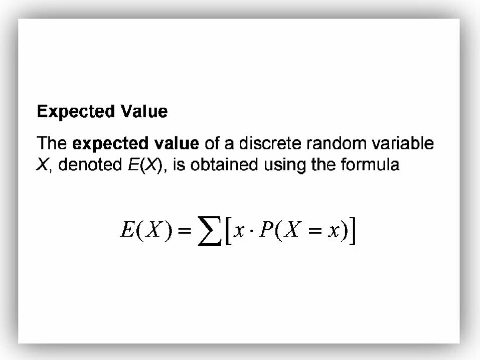
A random variable is a numerical measure of the outcome from a probability experiment, so its value is determined by chance. Random variables are denoted using letters such as X.
A discrete random variable is a random variable that has values that has either a finite number of possible values or a countable number of possible values.
A continuous random variable is a random variable that has an infinite number of possible values that is not countable.
EXAMPLE Distinguishing Between Discrete and Continuous Random Variables
Determine whether the following random variables are discrete or continuous. State possible values for the random variable.
(a) The number of light bulbs that burn out in a room of 10 light bulbs in the next year.
(b) The number of leaves on a randomly selected Oak tree.
(c) The length of time between calls to 911.
(d) A single die is cast. The number of pips showing on the die.
• We use capital letter , like X, to denote the random variable and use small letter to list the possible values of the random variable.
• Example. A single die is cast, X represent the number of pips showing on the die and the possible values of X are x=1,2,3,4,5,6.
A probability distribution provides the possible values of the random variable and their corresponding probabilities. A probability distribution can be in the form of a table, graph or mathematical formula.
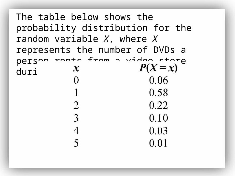
The table below shows the probability distribution for the random variable X, where X represents the number of DVDs a person rents from a video store during a single visit.
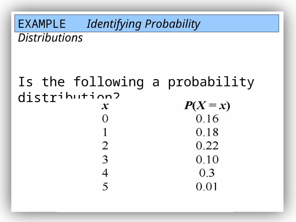
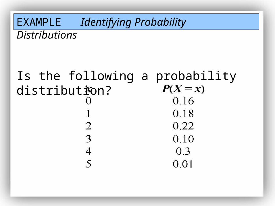
EXAMPLE Identifying Probability Distributions
Is the following a probability distribution?
EXAMPLE Identifying Probability Distributions
Is the following a probability distribution?
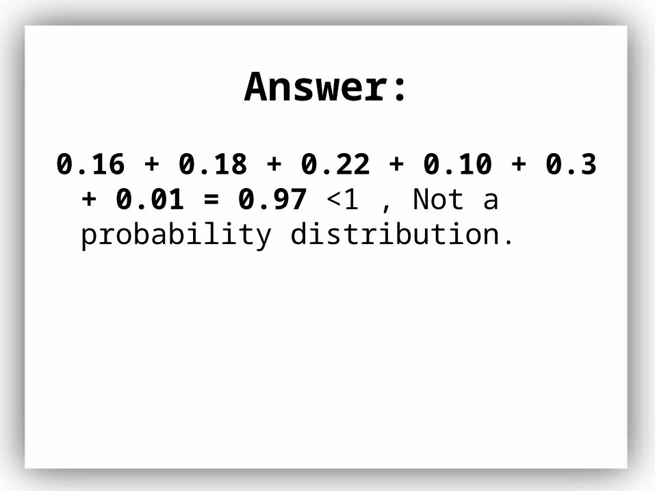
Answer:
0.16 + 0.18 + 0.22 + 0.10 + 0.3 + 0.01 = 0.97 <1 , Not a probability distribution.
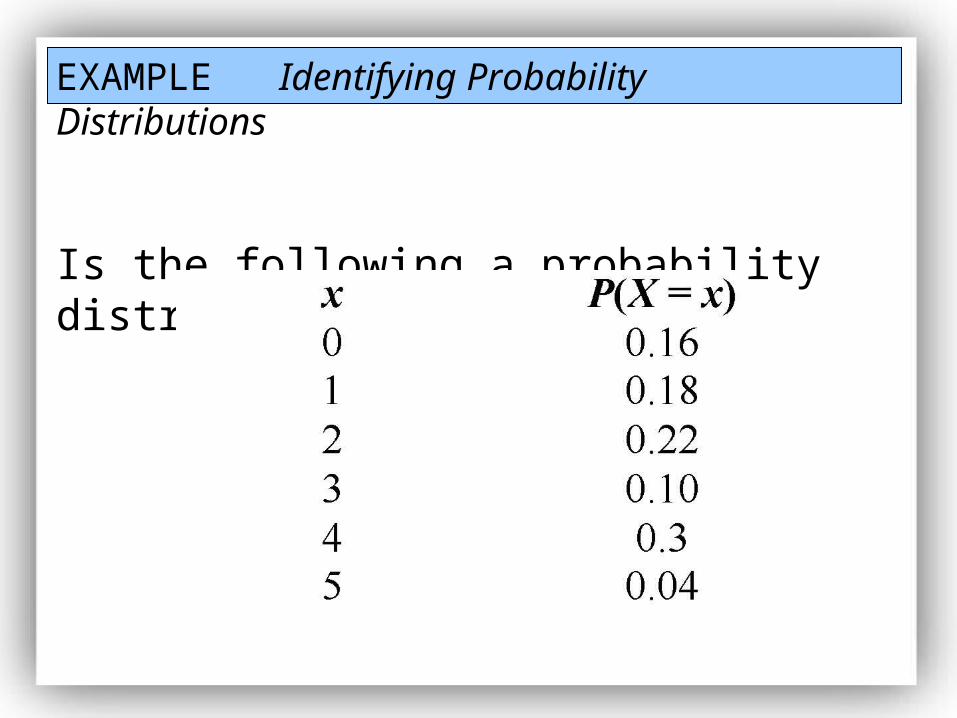
EXAMPLE Identifying Probability Distributions
Is the following a probability distribution?
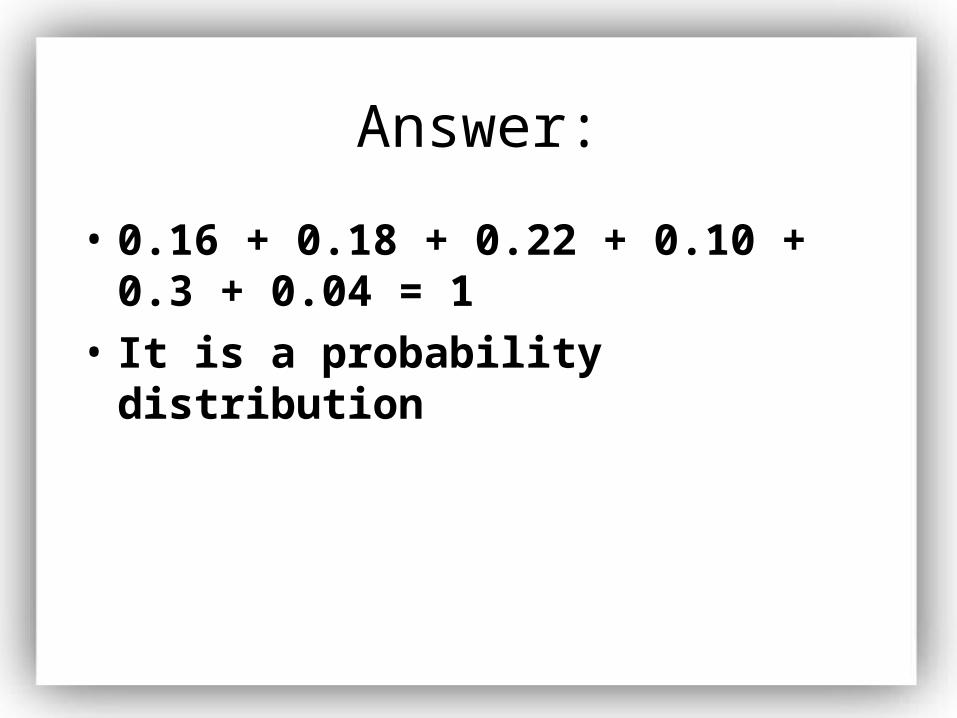
Answer:
• 0.16 + 0.18 + 0.22 + 0.10 + 0.3 + 0.04 = 1
• It is a probability distribution
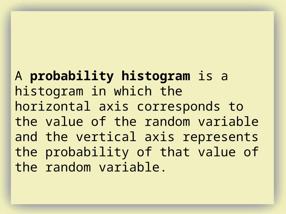
A probability histogram is a histogram in which the horizontal axis corresponds to the value of the random variable and the vertical axis represents the probability of that value of the random variable.
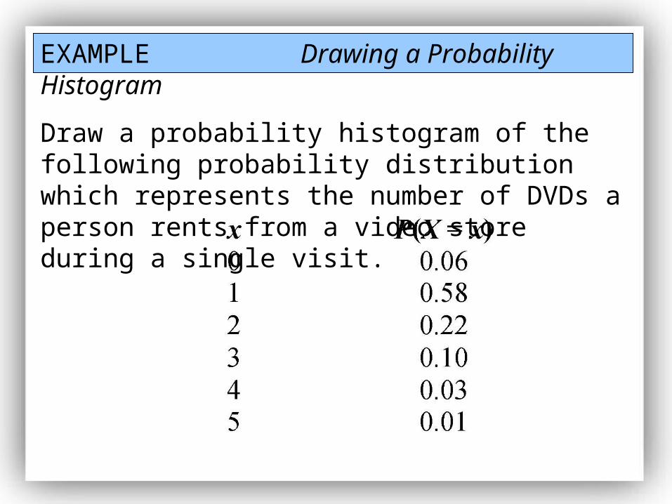
EXAMPLE Drawing a Probability Histogram
Draw a probability histogram of the following probability distribution which represents the number of DVDs a person rents from a video store during a single visit.
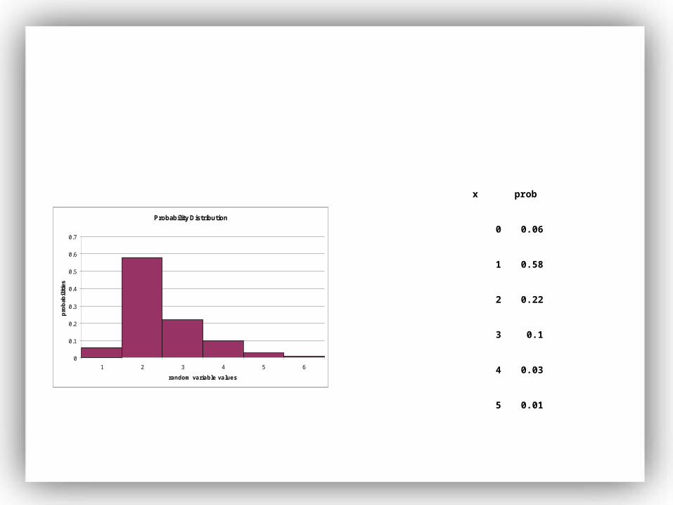
Probability Distribution
0
0.1
0.2
0.3
0.4
0.5
0.6
0.7
1 2 3 4 5 6
random variable values
pro
bab
ilit
ies
x prob
0 0.06
1 0.58
2 0.22
3 0.1
4 0.03
5 0.01
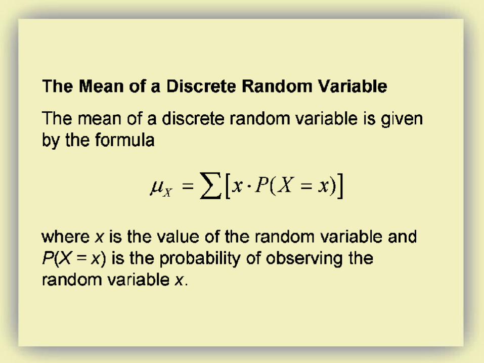
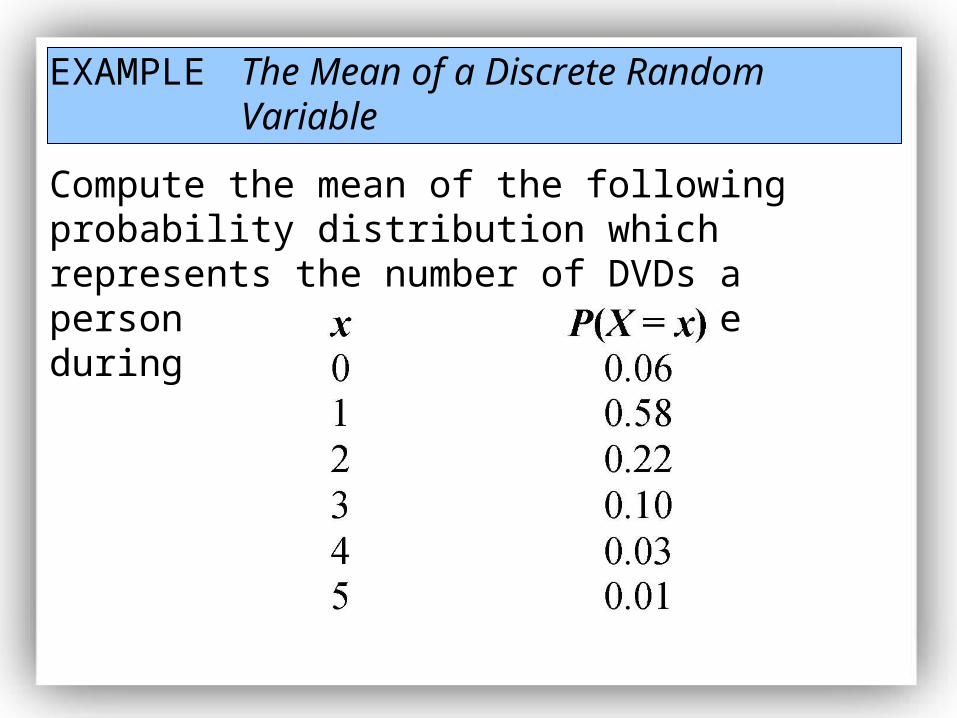
EXAMPLE The Mean of a Discrete Random Variable
Compute the mean of the following probability distribution which represents the number of DVDs a person rents from a video store during a single visit.
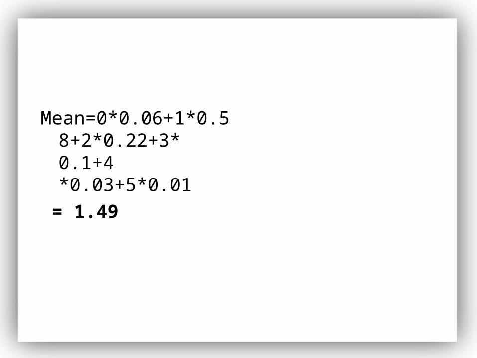
Mean=0*0.06+1*0.58+2*0.22+3* 0.1+4*0.03+5*0.01
= 1.49
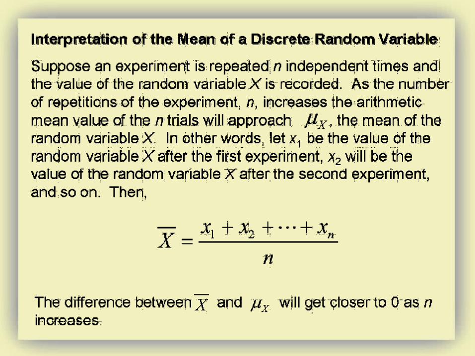
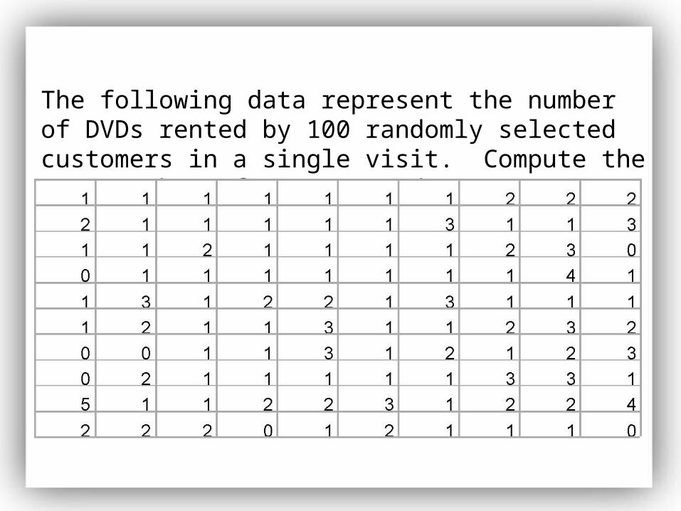
The following data represent the number of DVDs rented by 100 randomly selected customers in a single visit. Compute the mean number of DVDs rented.
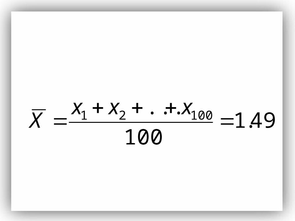
49.1100
... 10021
xxx
X
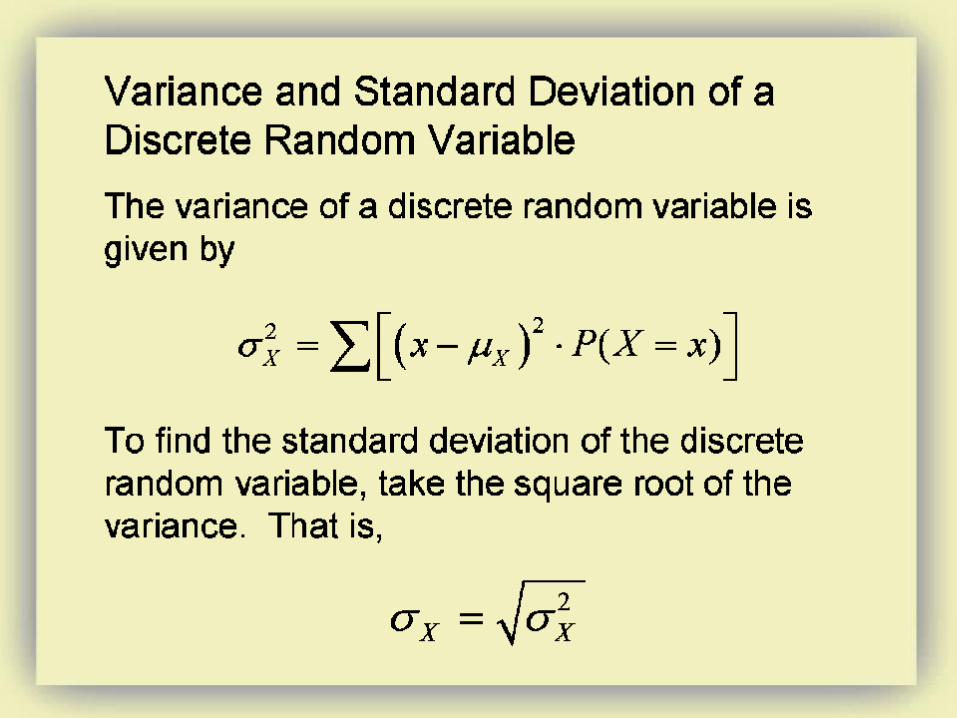
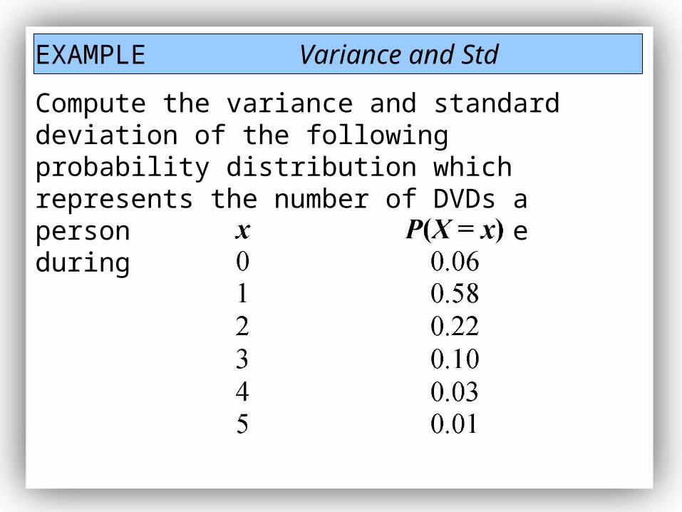
EXAMPLE Variance and Std
Compute the variance and standard deviation of the following probability distribution which represents the number of DVDs a person rents from a video store during a single visit.
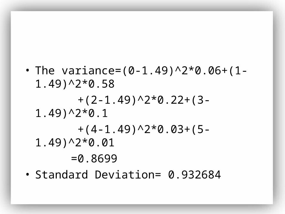
• The variance=(0-1.49)^2*0.06+(1-1.49)^2*0.58
+(2-1.49)^2*0.22+(3-1.49)^2*0.1
+(4-1.49)^2*0.03+(5-1.49)^2*0.01
=0.8699• Standard Deviation= 0.932684
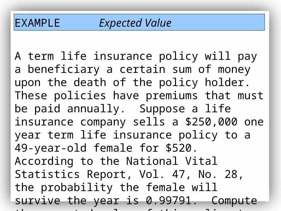
EXAMPLE Expected Value
A term life insurance policy will pay a beneficiary a certain sum of money upon the death of the policy holder. These policies have premiums that must be paid annually. Suppose a life insurance company sells a $250,000 one year term life insurance policy to a 49-year-old female for $520. According to the National Vital Statistics Report, Vol. 47, No. 28, the probability the female will survive the year is 0.99791. Compute the expected value of this policy to the insurance company.
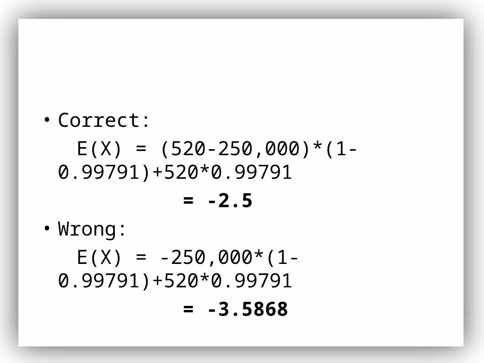
• Correct:
E(X) = (520-250,000)*(1- 0.99791)+520*0.99791
= -2.5
• Wrong:
E(X) = -250,000*(1-0.99791)+520*0.99791
= -3.5868
Chapter SixDiscrete Probability
Distributions
6.2
The Binomial Probability Distribution
Criteria for a Binomial Probability ExperimentCriteria for a Binomial Probability Experiment
An experiment is said to be a binomial experiment provided
1. The experiment is performed a fixed number of times. Each repetition of the experiment is called a trial.
2. The trials are independent. This means the outcome of one trial will not affect the outcome of the other trials.
3. For each trial, there are two mutually exclusive outcomes, success or failure.
4. The probability of success is fixed for each trial of the experiment.
Notation Used in the Notation Used in the Binomial Probability DistributionBinomial Probability Distribution
• There are n independent trials of the experiment
• Let p denote the probability of success so that 1 – p is the probability of failure.
• Let x denote the number of successes in n independent trials of the experiment. So, 0 < x < n.
EXAMPLE Identifying Binomial Experiments
Which of the following are binomial experiments?
(a) A player rolls a pair of fair die 10 times. The number X of 7’s rolled is recorded.
(b) The 11 largest airlines had an on-time percentage of 84.7% in November, 2001 according to the Air Travel Consumer Report. In order to assess reasons for delays, an official with the FAA randomly selects flights until she finds 10 that were not on time. The number of flights X that need to be selected is recorded.
(c ) In a class of 30 students, 55% are female. The instructor randomly selects 4 students. The number X of females selected is recorded.
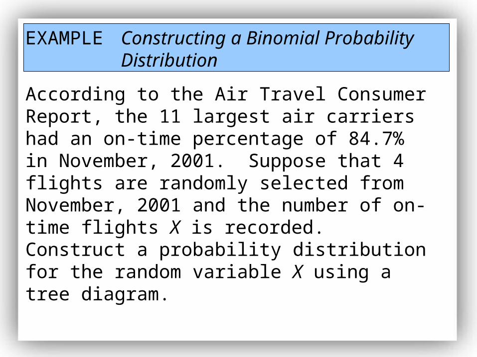
EXAMPLE Constructing a Binomial Probability Distribution
According to the Air Travel Consumer Report, the 11 largest air carriers had an on-time percentage of 84.7% in November, 2001. Suppose that 4 flights are randomly selected from November, 2001 and the number of on-time flights X is recorded. Construct a probability distribution for the random variable X using a tree diagram.
• X=(x1,x2,x3,x4)
• X=the number of on-time

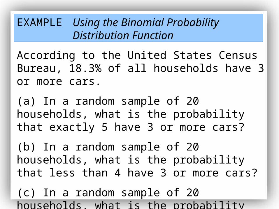
EXAMPLE Using the Binomial Probability Distribution Function
According to the United States Census Bureau, 18.3% of all households have 3 or more cars.
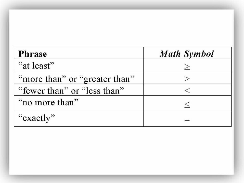
(a) In a random sample of 20 households, what is the probability that exactly 5 have 3 or more cars?
(b) In a random sample of 20 households, what is the probability that less than 4 have 3 or more cars?
(c) In a random sample of 20 households, what is the probability that at least 4 have 3 or more cars?
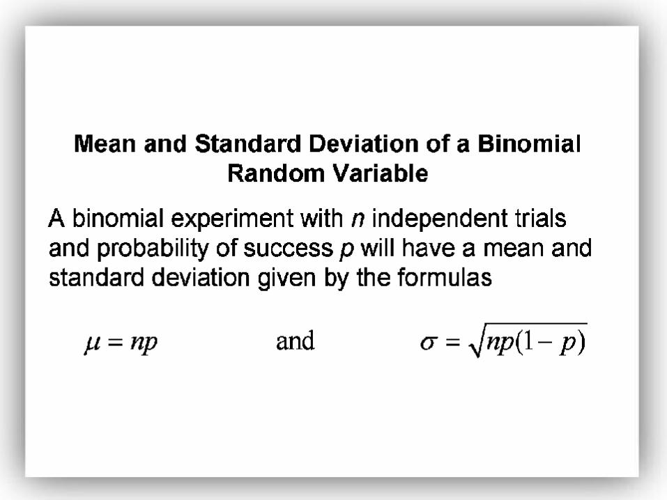
EXAMPLE Finding the Mean and Standard Deviation of a Binomial Random Variable
According to the United States Census Bureau, 18.3% of all households have 3 or more cars. In a simple random sample of 400 households, determine the mean and standard deviation number of households that will have 3 or more cars.
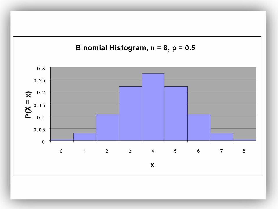
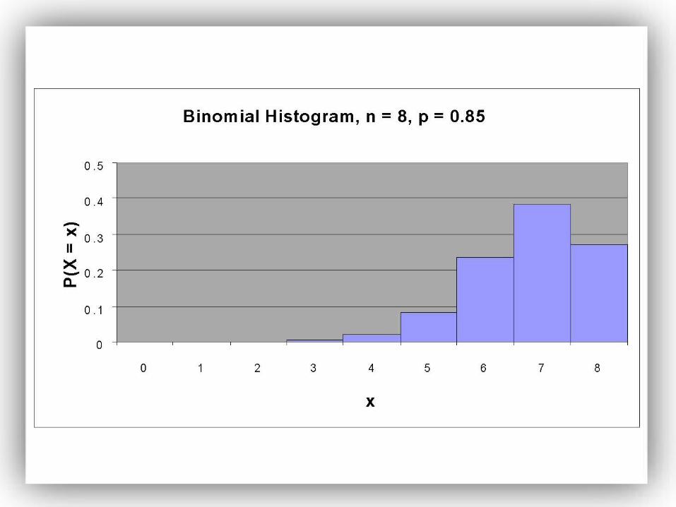
EXAMPLE Constructing Binomial Probability Histograms
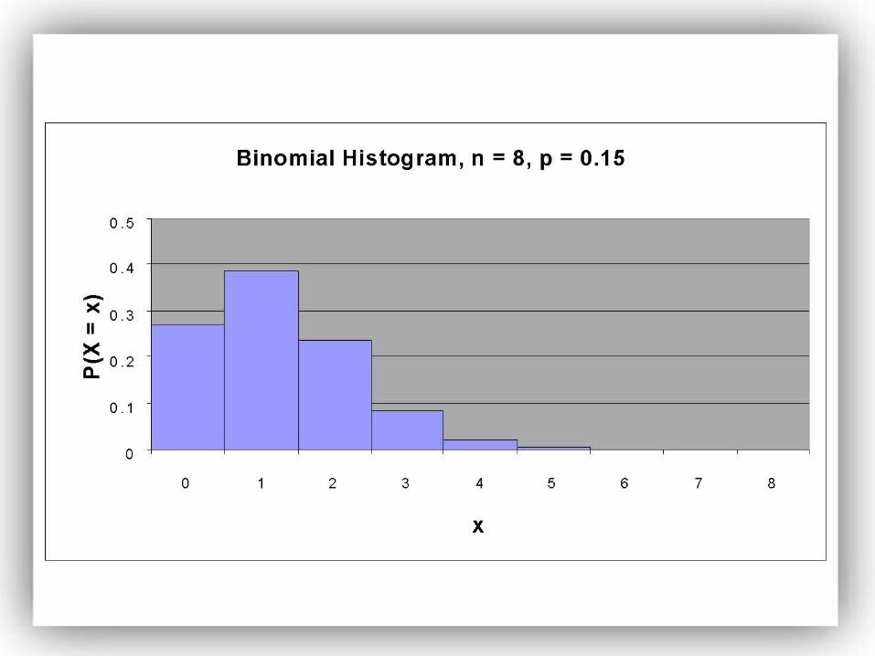
(a) Construct a binomial probability histogram with n = 8 and p = 0.15.
(b) Construct a binomial probability histogram with n = 8 and p = 0. 5.
(c) Construct a binomial probability histogram with n = 8 and p = 0.85.
For each histogram, comment on the shape of the distribution.
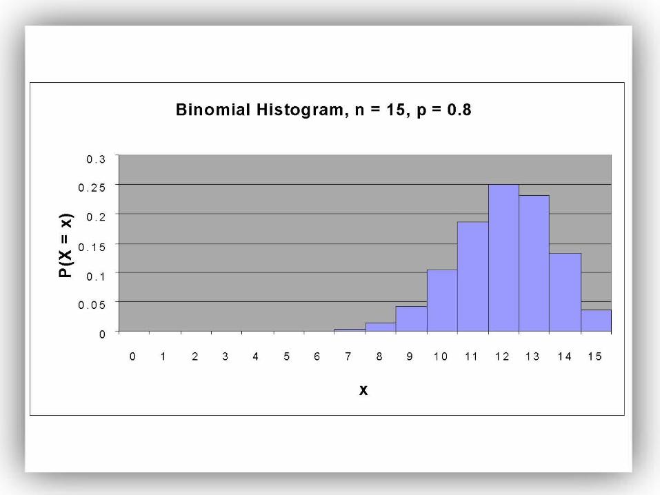
Construct a binomial probability histogram with n = 15 and p = 0.8. Comment on the shape of the distribution.
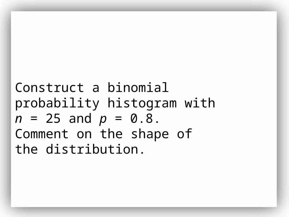
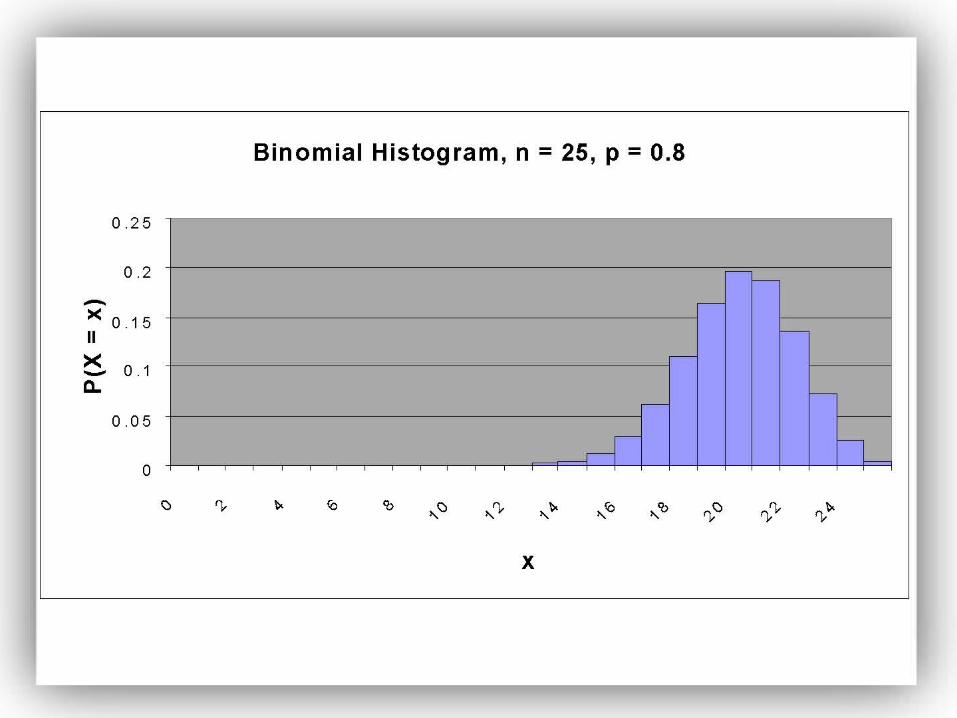
Construct a binomial probability histogram with n = 25 and p = 0.8. Comment on the shape of the distribution.
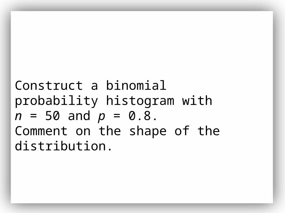
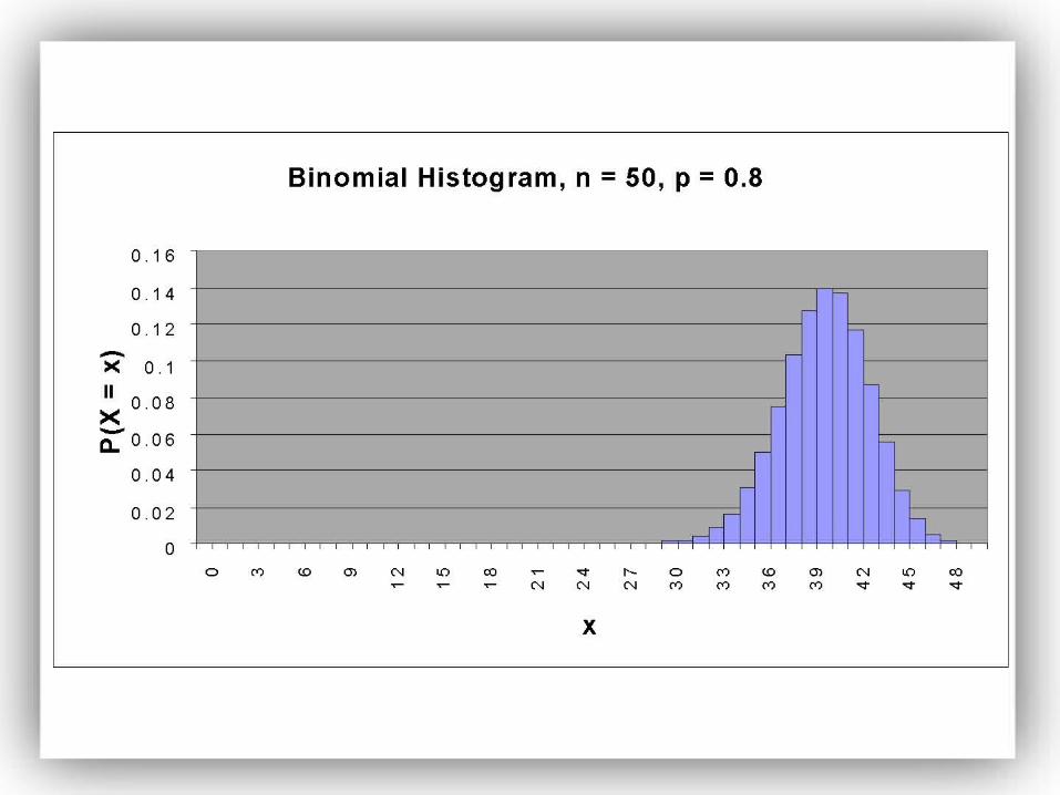
Construct a binomial probability histogram with n = 50 and p = 0.8. Comment on the shape of the distribution.

Construct a binomial probability histogram with n = 70 and p = 0.8. Comment on the shape of the distribution.
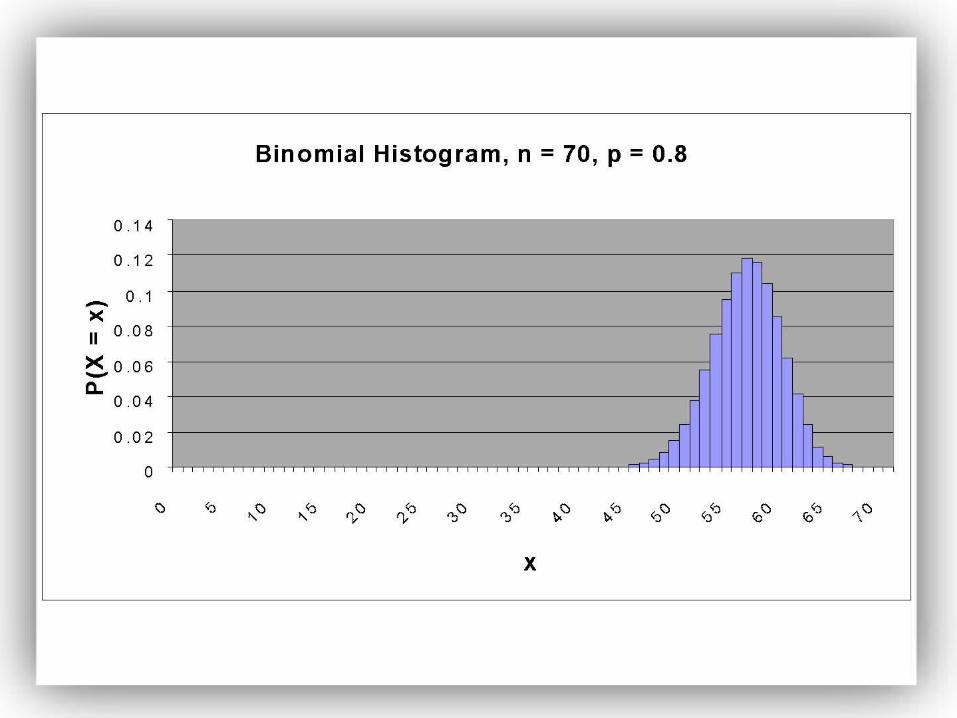
As the number of trials n in a binomial experiment increase, the probability distribution of the random variable X becomes bell-shaped. As a general rule of thumb, if np(1 – p) > 10, then the probability distribution will be approximately bell-shaped.
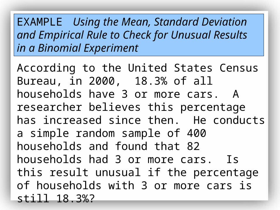
EXAMPLE Using the Mean, Standard Deviation and Empirical Rule to Check for Unusual Results in a Binomial Experiment
According to the United States Census Bureau, in 2000, 18.3% of all households have 3 or more cars. A researcher believes this percentage has increased since then. He conducts a simple random sample of 400 households and found that 82 households had 3 or more cars. Is this result unusual if the percentage of households with 3 or more cars is still 18.3%?
EXAMPLE Using the Binomial Probability Distribution Function to Perform Inference
According to the United States Census Bureau, in 2000, 18.3% of all households have 3 or more cars. A researcher believes this percentage has increased since then. He conducts a simple random sample of 20 households and found that 5 households had 3 or more cars.
Is this result unusual if the percentage of households with 3 or more cars is still 18.3%?

EXAMPLE Using the Binomial Probability Distribution Function to Perform Inference
According to the United States Census Bureau, in 2000, 18.3% of all households have 3 or more cars. One year later, the same researcher conducts a simple random sample of 20 households and found that 8 households had 3 or more cars.
Is this result unusual if the percentage of households with 3 or more cars is still 18.3%?
Chapter SixDiscrete Probability
DistributionsSection 6.3
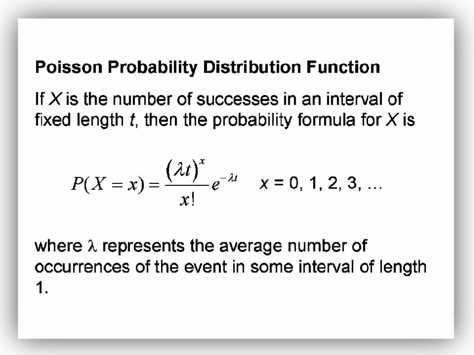
The Poisson Probability Distribution
A random variable X, the number of successes in a fixed interval, follows a Poisson process provided the following conditions are met
1. The probability of two or more successes in any sufficiently small subinterval is 0.
2. The probability of success is the same for any two intervals of equal length.
3. The number of successes in any interval is independent of the number of successes in any other interval provided the intervals are not overlapping.
EXAMPLE A Poisson Process
The Food and Drug Administration sets a Food Defect Action Level (FDAL) for various foreign substances that inevitably end up in the food we eat and liquids we drink. For example, the FDAL level for insect filth in chocolate is 0.6 insect fragments (larvae, eggs, body parts, and so on) per 1 gram.
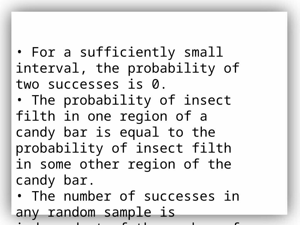
• For a sufficiently small interval, the probability of two successes is 0.• The probability of insect filth in one region of a candy bar is equal to the probability of insect filth in some other region of the candy bar.• The number of successes in any random sample is independent of the number of successes in any other random sample.

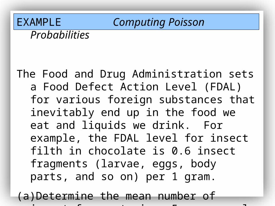
EXAMPLE Computing Poisson Probabilities
The Food and Drug Administration sets a Food Defect Action Level (FDAL) for various foreign substances that inevitably end up in the food we eat and liquids we drink. For example, the FDAL level for insect filth in chocolate is 0.6 insect fragments (larvae, eggs, body parts, and so on) per 1 gram.
(a)Determine the mean number of insect fragments in a 5 gram sample of chocolate.
(b) What is the standard deviation?
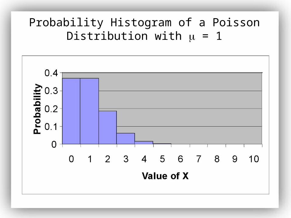
Probability Histogram of a Poisson Distribution with = 1
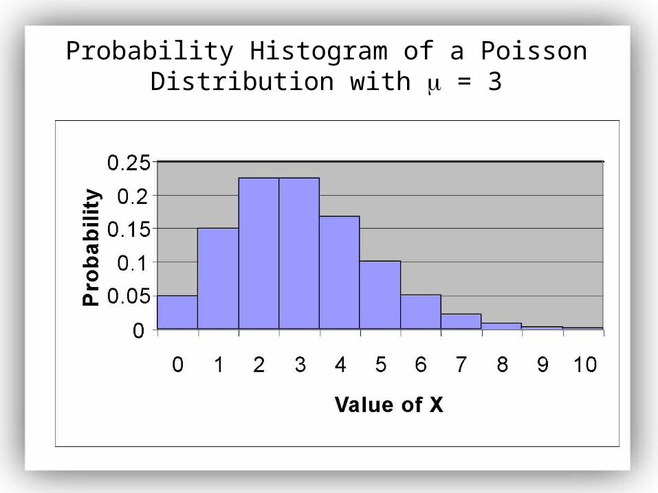
Probability Histogram of a Poisson Distribution with = 3
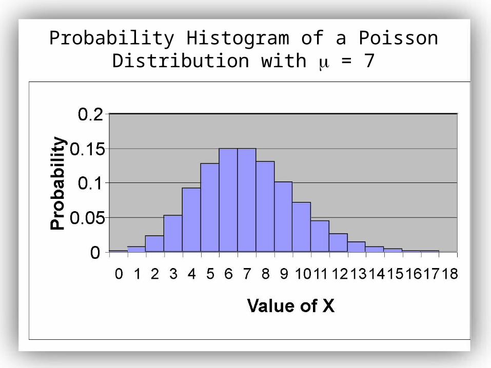
Probability Histogram of a Poisson Distribution with = 7
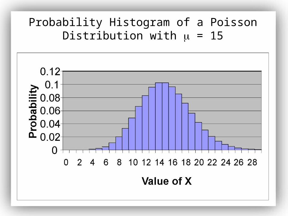
Probability Histogram of a Poisson Distribution with = 15

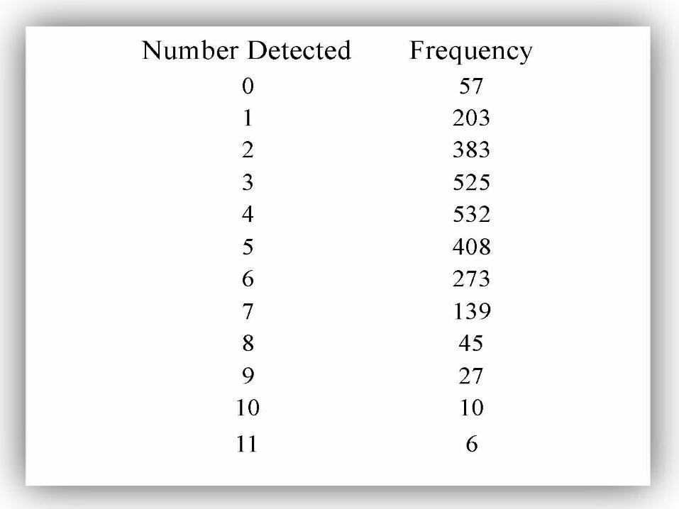
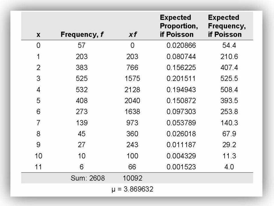
EXAMPLE Poisson Particles
In 1910, Ernest Rutherford and Hans Geiger recorded the number of -particles emitted from a polonium source in eighth-minute (7.5 second) intervals. The results are reported in the table on the next slide. Does a Poisson probability function accurately describe the number of -particles emitted?
Source: Rutherford, Sir Ernest; Chadwick, James; and Ellis, C.D.. Radiations from Radioactive Substances. London, Cambridge University Press, 1951, p. 172.
The Poisson probability distribution function can be used to approximate binomial probabilities provided the number of trials n > 100 and np < 10. In other words, the number of independent trials of the binomial experiment should be large and the probability of success should be small.
EXAMPLE Using the Poisson Distribution to Approximate Binomial Probabilities
According to the U.S. National Center for Health Statistics, 7.6% of male children under the age of 15 years have been diagnosed with Attention Deficit Disorder (ADD). In a random sample of 120 male children under the age of 15 years, what is the probability that at least 4 of the children have ADD?
Related Documents