Chapter Normal Probability Distributions 1 of 105 5 © 2012 Pearson Education, Inc. All rights reserved. Edited by Tonya Jagoe.

ChapterNormal Probability Distributions

1 of 105

5

© 2012 Pearson Education, Inc.All rights reserved.

Edited by Tonya Jagoe

Properties of Normal Distributions

Normal distribution

• A continuous probability distribution for a random variable, x.

• The most important continuous probability distribution in statistics.

• The graph of a normal distribution is called the normal curve.

x

© 2012 Pearson Education, Inc. All rights reserved. 2 of 105

Properties of Normal Distributions

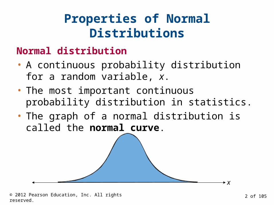
1. The mean, median, and mode are equal.

2. The normal curve is bell-shaped and is symmetric about the mean.

3. The total area under the normal curve is equal to 1.

4. The normal curve approaches, but never touches, the x-axis as it extends farther and farther away from the mean.

x

Total area = 1

μ© 2012 Pearson Education, Inc. All rights reserved. 3 of 105

Properties of Normal Distributions

5. Between μ – σ and μ + σ (in the center of the curve), the graph curves downward. The graph curves upward to the left of μ – σ and to the right of μ + σ. The points at which the curve changes from curving upward to curving downward are called the inflection points.

© 2012 Pearson Education, Inc. All rights reserved. 4 of 105

μ – 3σ μ + σμ – σ μ μ + 2σ μ + 3σμ – 2σ

Notice that the inflection points correspond to +/- 1 standard deviation from the mean.

Means and Standard Deviations

• A normal distribution can have any mean and any positive standard deviation.

• The mean gives the location of the line of symmetry.

• The standard deviation describes the spread of the data.

μ = 3.5σ = 1.5

μ = 3.5σ = 0.7

μ = 1.5σ = 0.7

© 2012 Pearson Education, Inc. All rights reserved. 5 of 105

Example: Understanding Mean and Standard Deviation

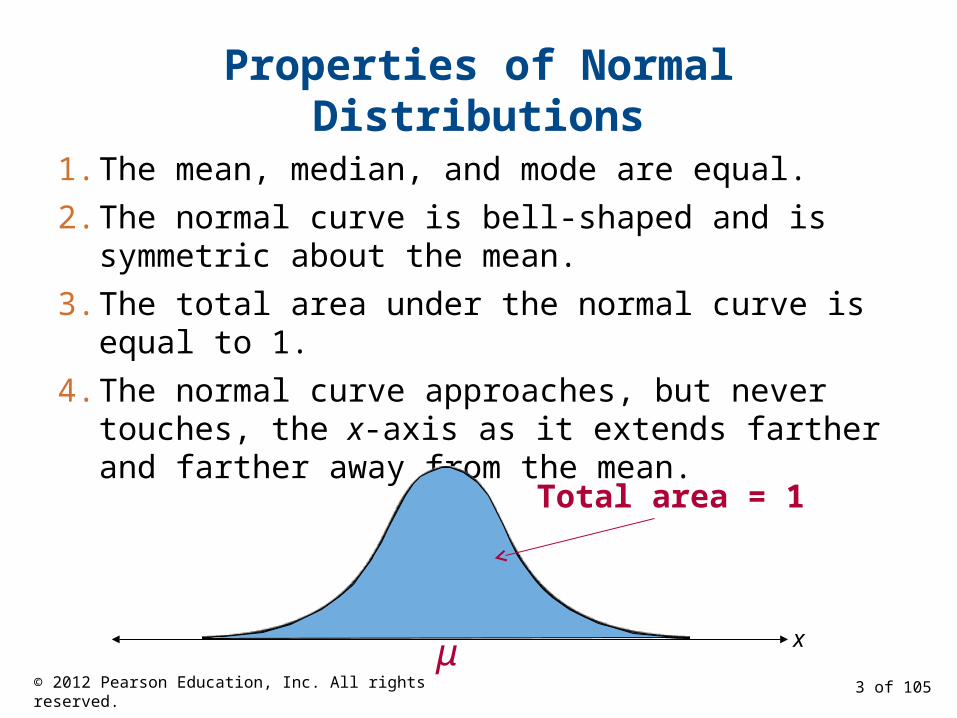
1. Which normal curve has the greater mean?

Solution:Curve A has the greater mean (The line of symmetry of curve A occurs at x = 15. The line of symmetry of curve B occurs at x = 12.)

© 2012 Pearson Education, Inc. All rights reserved. 6 of 105

Example: Understanding Mean and Standard Deviation

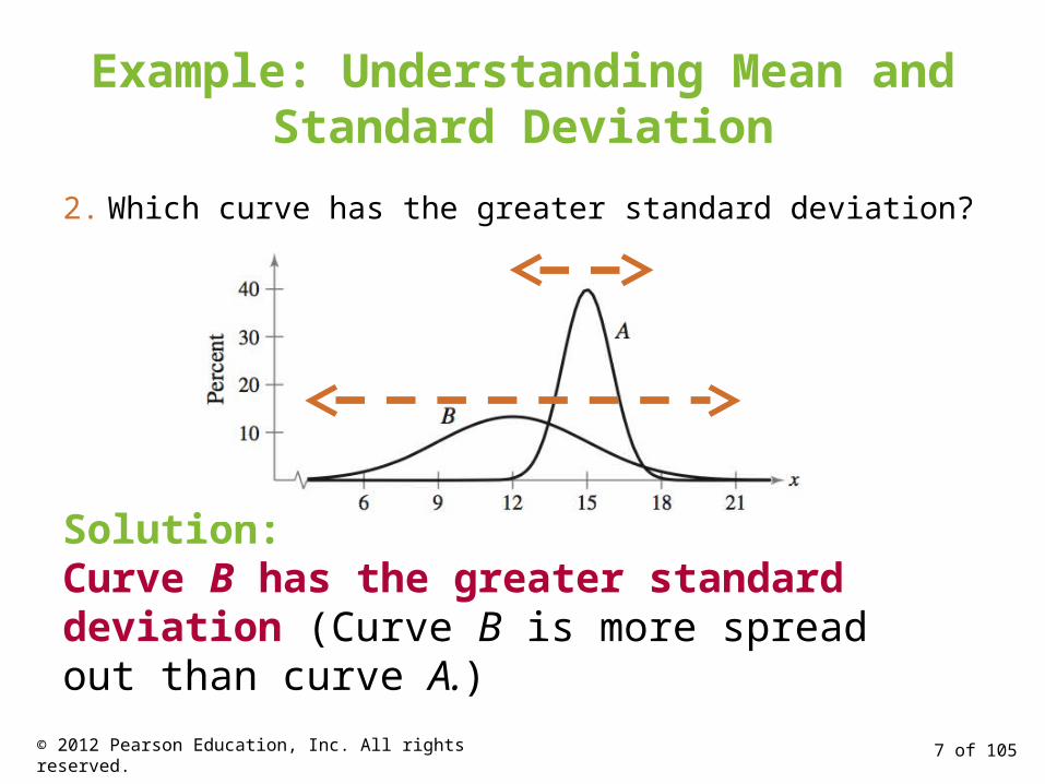
2. Which curve has the greater standard deviation?

Solution:Curve B has the greater standard deviation (Curve B is more spread out than curve A.)

© 2012 Pearson Education, Inc. All rights reserved. 7 of 105

Example: Interpreting Graphs

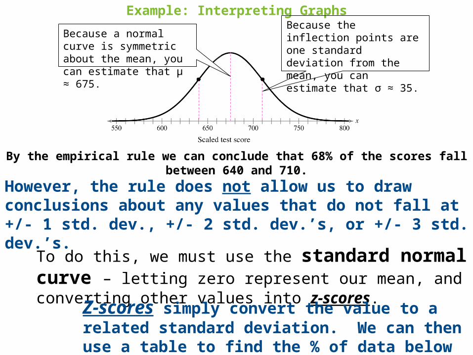
The scaled test scores for the New York State Grade 8 Mathematics Test are normally distributed. The normal curve shown below represents this distribution. What is the mean test score? Estimate the standard deviation.

Solution:

© 2012 Pearson Education, Inc. All rights reserved. 8 of 105

Because a normal curve is symmetric about the mean, you can estimate that μ ≈ 675.

Because the inflection points are one standard deviation from the mean, you can estimate that σ ≈ 35.

Example: Interpreting Graphs

Because a normal curve is symmetric about the mean, you can estimate that μ ≈ 675.

Because the inflection points are one standard deviation from the mean, you can estimate that σ ≈ 35.

By the empirical rule we can conclude that 68% of the scores fall between 640 and 710.

However, the rule does not allow us to draw conclusions about any values that do not fall at +/- 1 std. dev., +/- 2 std. dev.’s, or +/- 3 std. dev.’s.

To do this, we must use the standard normal curve – letting zero represent our mean, and converting other values into z-scores.

Z-scores simply convert the value to a related standard deviation. We can then use a table to find the % of data below that value.

The Standard Normal Distribution

Standard normal distribution

• A normal distribution with a mean of 0 and a standard deviation of 1.

–3 1–2 –1 0 2 3

z

Area = 1

z Value Mean

Standard deviation x

• Any x-value can be transformed into a z-score by using the formula

© 2012 Pearson Education, Inc. All rights reserved. 10 of 105

Properties of the Standard Normal Distribution

1. The cumulative area is the area under the curve to the left of the value.

2. The cumulative area is close to 0 for z-scores close to z = –3.49.

3. The cumulative area increases as the z-scores increase.

z = –3.49

Area is close to 0

z

–3 1–2 –1 0 2 3

© 2012 Pearson Education, Inc. All rights reserved. 11 of 105

Think back to the empirical rule: the % of data falling below -3 std. dev.’s was 0.15%; therefore, the % falling below -3.49 would be even less, and very close to zero.

Again, think back to the empirical rule: the % of data falling < -3 std. dev.’s was 0.15%, < -2 std. dev.’s was 2.5%, < -1 std. dev.16%, < +1 std. dev. 66%, < +2 std. dev. 97.5%, and < +3 std. dev. 99.85%.

z = 3.49

Area is close to 1

Properties of the Standard Normal Distribution

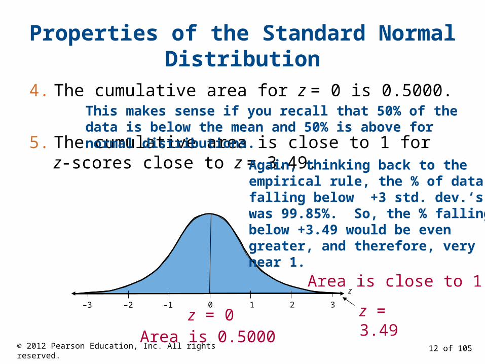
4. The cumulative area for z = 0 is 0.5000.

5. The cumulative area is close to 1 for z-scores close to z = 3.49.

Area is 0.5000z = 0

z

–3 1–2 –1 0 2 3

© 2012 Pearson Education, Inc. All rights reserved. 12 of 105

This makes sense if you recall that 50% of the data is below the mean and 50% is above for normal distributions.

Again, thinking back to the empirical rule, the % of data falling below +3 std. dev.’s was 99.85%. So, the % falling below +3.49 would be even greater, and therefore, very near 1.

Example: Using The Standard Normal Table

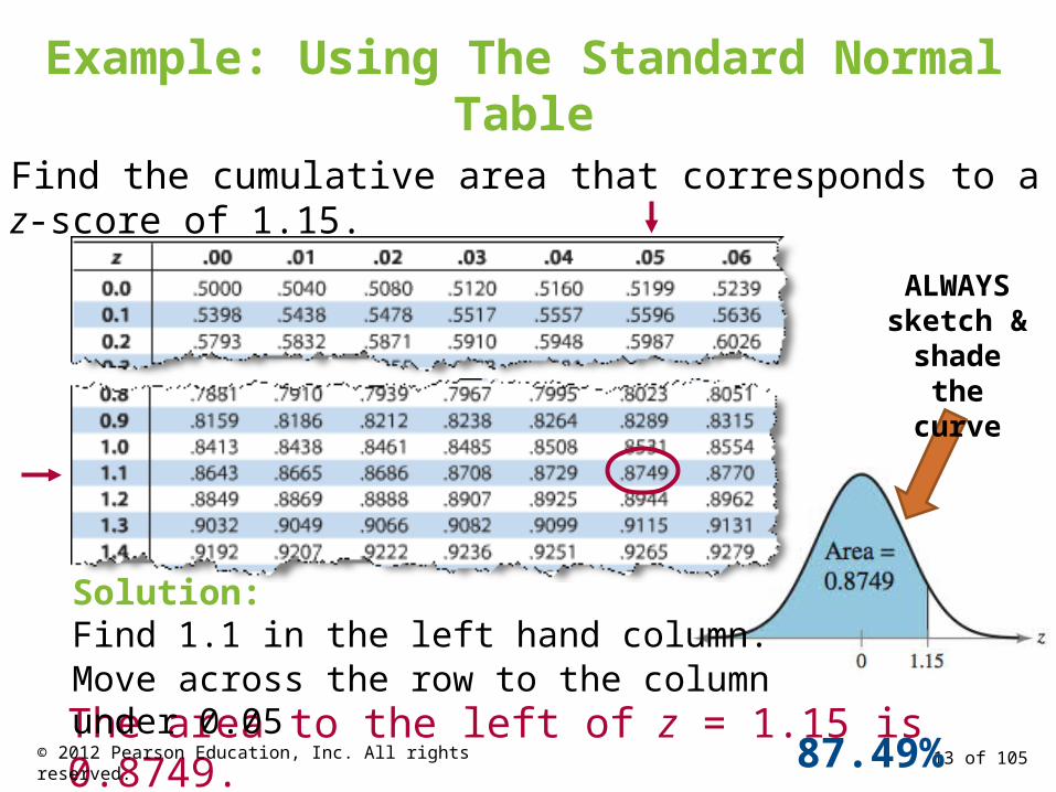
Find the cumulative area that corresponds to a z-score of 1.15.

The area to the left of z = 1.15 is 0.8749.Move across the row to the column under 0.05

Solution:Find 1.1 in the left hand column.

© 2012 Pearson Education, Inc. All rights reserved. 13 of 105

ALWAYS sketch & shade the

curve

87.49%

Example: Using The Standard Normal Table

Find the cumulative area that corresponds to a z-score of –0.24.

Solution:Find –0.2 in the left hand column.

The area to the left of z = –0.24 is 0.4052.© 2012 Pearson Education, Inc. All rights reserved. 14 of 105

Move across the row to the column under 0.04

ALWAYS sketch & shade the

curve

_____%

Finding Areas Under the Standard Normal Curve

1. Sketch the standard normal curve and shade the appropriate area under the curve.

2. Find the area by following the directions for each case shown.a. To find the area to the left of z, find the area that

corresponds to z in the Standard Normal Table.

1. Use the table to find the area for the z-score

2. The area to the left of z = 1.23 is 0.8907

© 2012 Pearson Education, Inc. All rights reserved. 15 of 105

89.07%

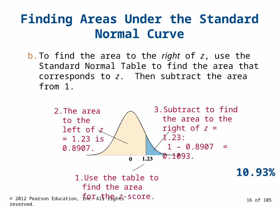
Finding Areas Under the Standard Normal Curve

b. To find the area to the right of z, use the Standard Normal Table to find the area that corresponds to z. Then subtract the area from 1.

3. Subtract to find the area to the right of z = 1.23: 1 – 0.8907 = 0.1093.

1. Use the table to find the area for the z-score.

2. The area to the left of z = 1.23 is 0.8907.

© 2012 Pearson Education, Inc. All rights reserved. 16 of 105

10.93%

Finding Areas Under the Standard Normal Curve

c. To find the area between two z-scores, find the area corresponding to each z-score in the Standard Normal Table. Then subtract the smaller area from the larger area.

4. Subtract to find the area of the region between the two z-scores: 0.8907 – 0.2266 = 0.6641.3. The area to the

left of z = –0.75 is 0.2266.

2. The area to the left of z = 1.23 is 0.8907.

1. Use the table to find the area for the z-scores.

© 2012 Pearson Education, Inc. All rights reserved. 17 of 105

66.41%

Example: Finding Area Under the Standard Normal Curve

Find the area under the standard normal curve to the left of z = –0.99.

From the Standard Normal Table, the area is equal to 0.1611.

–0.99 0z

0.1611

Solution:

© 2012 Pearson Education, Inc. All rights reserved. 18 of 10516.11%

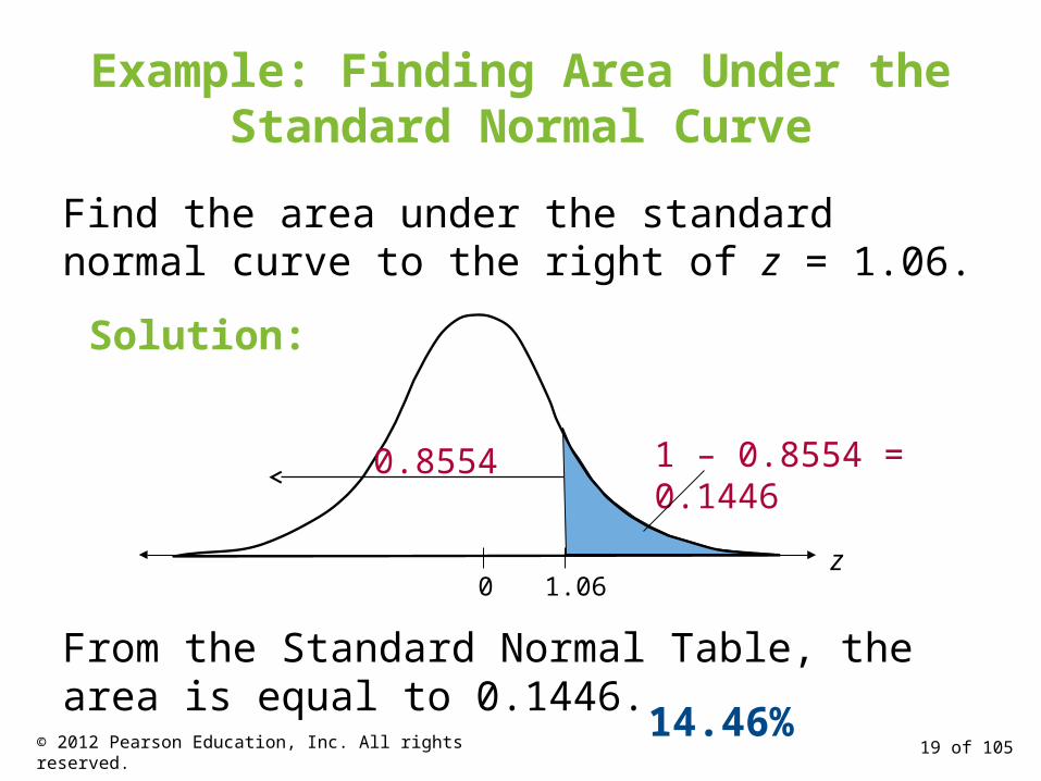
Example: Finding Area Under the Standard Normal Curve

Find the area under the standard normal curve to the right of z = 1.06.

From the Standard Normal Table, the area is equal to 0.1446.

1 – 0.8554 = 0.1446

1.060z

Solution:

0.8554

© 2012 Pearson Education, Inc. All rights reserved. 19 of 10514.46%

Find the area under the standard normal curve between z = –1.5 and z = 1.25.

Example: Finding Area Under the Standard Normal Curve

From the Standard Normal Table, the area is equal to 0.8276.

1.250z

–1.50

0.89440.0668

Solution:0.8944 – 0.0668 = 0.8276

© 2012 Pearson Education, Inc. All rights reserved. 20 of 10582.76%