CHAPTER I INTRODUCTION AND REVIEW OF …shodhganga.inflibnet.ac.in/bitstream/10603/46/4/chapter 1...1 CHAPTER I INTRODUCTION AND REVIEW OF LITERATURE 1.1 INTRODUCTION This chapter

1

CHAPTER I

INTRODUCTION AND REVIEW OF LITERATURE

1.1 INTRODUCTION

This chapter presents a brief history of options, its growth and its

importance in global and Indian Financial, and Commodities Markets. Further it

includes statement of the problem, need for the study, research objectives, the

review of literature related to the basic formulation of the Black - Scholes (BS)

model, and the findings of empirical verification done by other researchers.

Option is a financial instrument whose value depends upon the value of

the underlying assets. Option itself has no value without underlying assets.

Option gives the right to the buyer either to sell or to buy the specified

underlying assets for a particular price (Exercise / Strike price) on or before a

particular date (expiration date). If the right is to buy, it is known as “call option”

and if the right is to sell, it is called as “put option”. The buyer of the option has

the right but no obligation either to buy or to sell. The option buyer has to

exercise the option on or before the expiration date, otherwise, the option

expires automatically at the end of the expiration date. Hence, options are also

known as contingent claims.

Such an instrument is extensively used in share markets, money

markets, and commodity markets to hedge the investment risks and acts as

financial leverage investment. Option is a kind of derivative instruments along

with forwards, futures and swaps, which are used for managing risk of the

investors. Though derivatives are theoretically risk management tools and

leveraged investment tools, most use them as speculative tools.

Though the derivatives were very old as early as 1630s, the exchange-

traded derivative market was introduced during 1970s. 1973 marked the

2

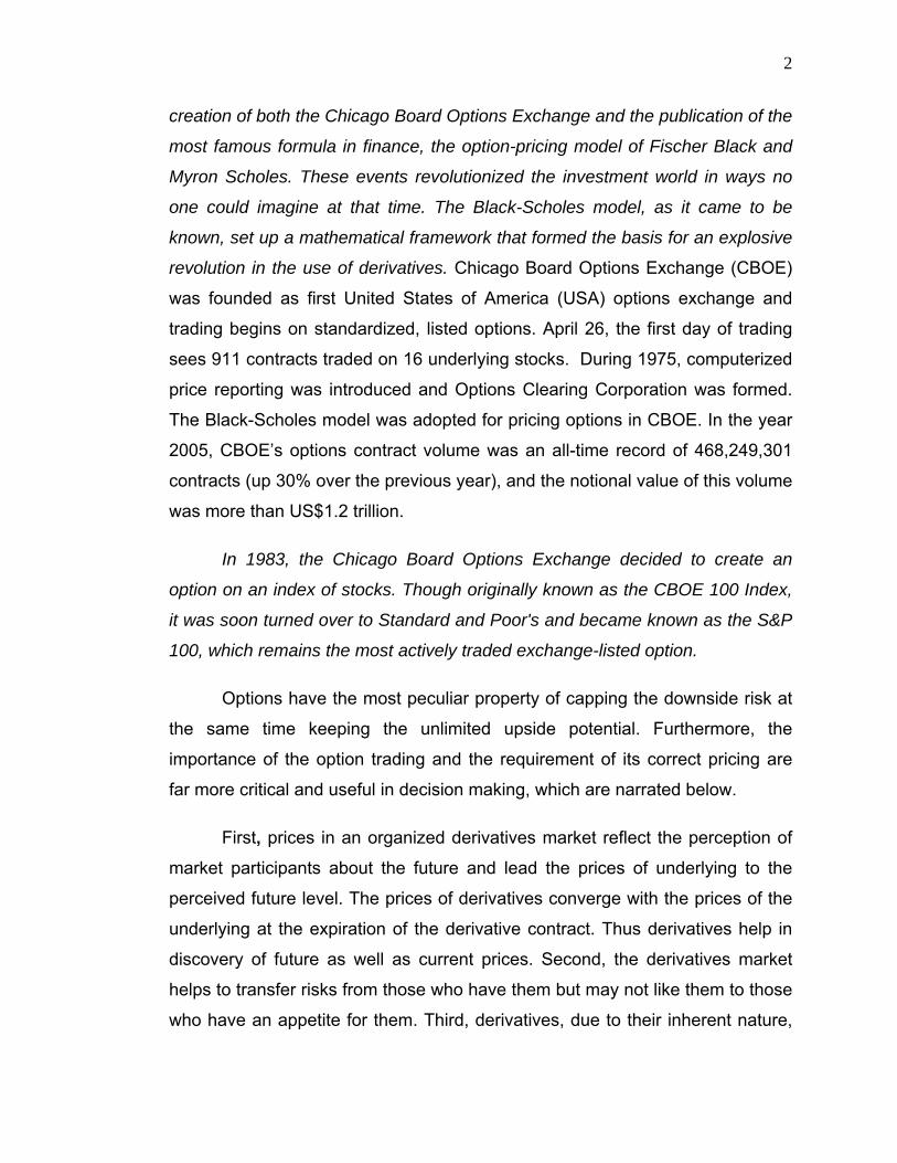
creation of both the Chicago Board Options Exchange and the publication of the

most famous formula in finance, the option-pricing model of Fischer Black and

Myron Scholes. These events revolutionized the investment world in ways no

one could imagine at that time. The Black-Scholes model, as it came to be

known, set up a mathematical framework that formed the basis for an explosive

revolution in the use of derivatives. Chicago Board Options Exchange (CBOE)

was founded as first United States of America (USA) options exchange and

trading begins on standardized, listed options. April 26, the first day of trading

sees 911 contracts traded on 16 underlying stocks. During 1975, computerized

price reporting was introduced and Options Clearing Corporation was formed.

The Black-Scholes model was adopted for pricing options in CBOE. In the year

2005, CBOE’s options contract volume was an all-time record of 468,249,301

contracts (up 30% over the previous year), and the notional value of this volume

was more than US$1.2 trillion.

In 1983, the Chicago Board Options Exchange decided to create an

option on an index of stocks. Though originally known as the CBOE 100 Index,

it was soon turned over to Standard and Poor's and became known as the S&P

100, which remains the most actively traded exchange-listed option.

Options have the most peculiar property of capping the downside risk at

the same time keeping the unlimited upside potential. Furthermore, the

importance of the option trading and the requirement of its correct pricing are

far more critical and useful in decision making, which are narrated below.

First, prices in an organized derivatives market reflect the perception of

market participants about the future and lead the prices of underlying to the

perceived future level. The prices of derivatives converge with the prices of the

underlying at the expiration of the derivative contract. Thus derivatives help in

discovery of future as well as current prices. Second, the derivatives market

helps to transfer risks from those who have them but may not like them to those

who have an appetite for them. Third, derivatives, due to their inherent nature,

3

are linked to the underlying cash markets. With the introduction of derivatives,

the underlying market witness higher trading volumes, because more players

participated who would not otherwise participate for lack of an arrangement to

transfer risk. Fourth, the speculative trades shift to a more controlled

environment of derivatives market. In the absence of an organized derivatives

market, speculators trade in the underlying cash markets. Margining, monitoring

and surveillance of the activities of various participants become extremely

difficult in these kinds of mixed markets. Fifth, an important incidental benefit

that flows from derivatives trading is that it acts as a catalyst for new

entrepreneurial activity. The derivatives have a history of attracting many bright,

creative, well-educated people with an entrepreneurial attitude. They often

energize others to create new businesses, new products and new employment

opportunities, the benefit of which are immense. Finally, derivatives markets

help increase savings and investment in the long run. Transfer of risk enables

market participants to expand their volume of activity.

In India, derivatives trading was introduced Index Futures Contracts

from June 2000 and stock option trading in July 2001 grown very fast to reach

an average daily turnover of derivatives at NSE, at Rs. 33,745 crores during

May 2006 as against cash markets turnover of about Rs. 9202.15 crores (as on

May 2006), which indicates the importance of the derivatives. Normally, the

derivative turnover is three to four times the cash market turnover in India.

Option, being one of the derivatives is a unique type of hedging tool.

Black – Scholes formula after mesmerize the western countries also entered

into in Indian option market.

4

1.2 OPTION BASICS

1.2.1 OPTION BASICS

1.2.1.1 Options

An option is a contract to buy or sell a specific financial product officially

known as the option's underlying instrument or underlying assets. For

exchange-traded equity options, the underlying instruments are stocks of listed

companies. The contract itself is very precise. It establishes a specific price,

called the strike price, at which the contract may be exercised or acted on and it

has an expiration date. When an option expires, it no longer has value and no

longer exists. Option is known as security, or contingent claim, or contract, or

derivative security or simply derivative. An option gives its holder the right to

purchase (sell), a specified quantity (lot size) of an underlying asset for a

specified price (exercise price or strike price) on or before some specified date

called expiration date, but the holder has no obligation to purchase (sell).

1.2.1.2 Types of Options

Options come in two varieties, calls and puts, and you can buy or sell

either type. You make those choices - whether to buy or sell and whether to

choose a call or a put - based on what you want to achieve as an options

investor. Call option gives its holder the right to purchase the underlying assets.

Put option gives it holder the right to sell the underlying assets.

1.2.1.3 Option terminology

1. Index options: These options have the index as the underlying. Some

options are European while others are American. Like index futures

contracts, index options contracts are also cash settled.

5

2. Stock options: Stock options are options on individual stocks. Options

currently trade on over 500 stocks in the USA. A contract gives the holder

the right to buy or sell shares at the specified price.

3. Buyer of an option: The buyer of an option is the one who by paying the

option premium buys the right but not the obligation to exercise his option

on the seller/writer.

4. Writer of an option: The writer of a call/put option is the one who receives

the option premium and is thereby obliged to sell/buy the asset if the buyer

exercises on him.

5. Call option: A call option gives the holder the right but not the obligation to

buy an asset on a certain date for a certain price.

6. Put option: A put option gives the holder the right but not the obligation to

sell an asset on a certain date for a certain price.

7. Option price: Option price is the price which the option buyer pays to the

option seller. It is also referred to as the option premium.

8. Expiration date: The date specified in the options contract is known as the

expiration date / the exercise date /the strike date or the maturity.

9. Strike price: The price specified in the options contract is known as the

strike price or the exercise price.

10. American options: American options are options that can be exercised at

any time up to the expiration date. Most exchange-traded options are

American.

11. European options: European options are options that can be exercised only

on the expiration date itself. European options are easier to analyze than

6

American options, and properties of an American option are frequently

deduced from those of its European counterpart.

12. In-the-money option: An in-the-money (ITM) option is an option that would

lead to a positive cash flow to the holder if it were exercised immediately.

A call option on the index is said to be in-the-money when the current

index stands at a level higher than the strike price (i.e. spot price strike

price). If the index is much higher than the strike price, the call is said to be

deep ITM. In the case of a put, the put is ITM if the index is below the

strike price.

13. At-the-money option: An at-the-money (ATM) option is an option that

would lead to zero cash flow if it were exercised immediately. An option on

the index is at-the-money when the current index equals the strike price

(i.e. spot price = strike price).

14. Out-of-the-money option: An out-of-the-money (OTM) option is an option

that would lead to a negative cash flow it was exercised immediately. A

call option on the index is out-of-the-money when the current index stands

at a level which is less than the strike price (i.e. spot price strike price). If

the index is much lower than the strike price, the call is said to be deep

OTM. In the case of a put, the put is OTM if the index is above the strike

price.

15. Intrinsic value of an option: The option premium can be broken down into

two components – intrinsic value and time value. The intrinsic value of a

call is the difference between stock price and the strike price, if it is ITM. If

the call is OTM, its intrinsic value is zero. Putting it another way, the

intrinsic value of a call is Max [0, St – X] which means the intrinsic value of

a call is the greater of 0 or (St – X) Similarly, the intrinsic value of a put is

Max [0, X - St], i.e. the greater of 0 or (X - St) where X is the strike price

and St is the spot price.

7

16. Time value of an option: The time value of an option is the difference

between its premium and its intrinsic value. Both calls and puts have time

value. An option that is OTM or ATM has only time value. Usually, the

maximum time value exists when the option is ATM. The longer the time to

expiration, the greater is an option’s time value. At expiration, an option

should have no time value.

1.2.1.4 Option Pricing:

The price of the option is determined by many methods like binomial

method, Black Scholes option pricing formula, Volatility jump model etc. out of

which the Black Scholes option pricing model is most popular and widely used

through out the world. It is based on the assumption that the stock prices as per

continuous – time, continuous – variable stochastic Markov process.

Markov process states that the future value of stock price depends only on the

present value not on the history of the variable. The Markov property implies

that the probability distribution of the stock prices at any particular future time is

not dependent on the path followed by the price in the past. The Markov

property of the stock prices is consistent with the weak form of market

efficiency.

The variables and the parameters that determine the call option price are

diagrammatically given in Figure 1.1.

8

FIGURE 1.1

RISK FREE INTEREST

RATE R

VOLATILITY OF

THE STOCK RETURNS

σ

CURRENT

STOCK PRICE So

EXERCISE

PRICE X

LIFE PERIOD OF OPTION

T

OPTION PRICE

CO

FACTORS THAT AFFECT CALL OPTION PRICE

Future is uncertain and must be

istribu

expressed in terms of probability

d tions. The probability distribution of the price at any particular future time

is not dependent on the particular path followed by the price in the past. This

states that the present price of a stock impounds all the information contained in

a record of past prices. If the weak form of market efficiency were not true,

technical analysts could make above-average returns by interpreting charts of

the past history of stock prices. There is very little evidence that they are in fact

able to get above-average returns.

9

It is competition in the marketplace that tends to ensure that weak-form

market efficiency holds. There are many, many investors watching the stock

market closely. Trying to make a profit from it, leads to a situation where a stock

price, at any given time, reflects the information in past prices. Assume that it

was discovered a particular pattern in stock prices, which always gave a 65%

chance of subsequent steep price rises. Investors would attempt to buy a stock

as soon as the pattern was observed, and demand for the stock would

immediately rise. This would lead to an immediate rise in its price and the

observed effect would be eliminated, as would any profitable trading

opportunities.

1.2.2 OPTION AND THE STOCK MARKET

1.2.2.1 Market Efficiency

The derivatives make the stock market more efficient. The spot, future

and option markets are inextricably linked. Since it is easier and cheaper to

trade in derivatives, it is possible to exploit arbitrage opportunities quickly, and

keep the prices in alignment. Hence these markets help ensure that prices of

the underlying asset reflect true values.

Options can be used in a variety of ways to profit from a rise or fall in the

underlying asset market. The most basic strategies employ put and call options

as a low capital means of garnering a profit on market movements, known as

leveraging. Option route enable one to control the shares of a specific company

without tying up a large amount of capital in the trading account. A small portion

of money say, 20% (margin) is sufficient to get the underlying asset worth 100

percentages. Options can also be used as insurance policies in a wide variety

of trading scenarios. One, probably, has insurance on his / her car or house

because it is the responsible act and safe thing to do. Options provide the same

kind of safety net for trades and investments already committed, which is known

as hedging.

10

The amazing versatility that an option offers in today's highly volatile

markets is welcome relief from the uncertainties of traditional investing

practices. Options can be used to offer protection from a decline in the market

price of available underlying stocks or an increase in the market price of

uncovered underlying stock. Options can enable the investor to buy a stock at a

lower price, sell a stock at a higher price, or create additional income against a

long or short stock position. One can also uses option strategies to profit from a

movement in the price of the underlying asset regardless of market direction.

There are three general market directions: market up, market down, and

market sideways. It is important to assess potential market movement when

you are placing a trade. If the market is going up, you can buy calls, sell puts or

buy stocks. Does one have any other available choices? Yes, one can combine

long and short options and underlying assets in a wide variety of strategies.

These strategies limit your risk while taking advantage of market movement.

The following tables show the variety of options strategies that can be

applied to profit on market movement:

Bullish Limited Risk Strategies

Bullish Unlimited Risk Strategies

Bearish Limited Risk Strategies

Buy Call

Bull Call Spread

Bull Put Spread

Call Ratio Back spread

Buy Stock

Sell Put

Covered Call

Call Ratio Spread

Buy Put

Bear Put Spread

Bear Call Spread

Put Ratio Back spread

11

Bearish Unlimited Risk Strategies

Neutral Limited Risk Strategies

Neutral Unlimited Risk Strategies

Sell Stock

Sell Call

Covered Put

Put Ratio Spread

Long Straddle

Long Strangle

Long Synthetic Straddle

Put Ratio Spread

Long Butterfly

Long Condor

Long Iron Butterfly

Short Straddle

Short Strangle

Call Ratio Spread

Put Ratio Spread

It is of paramount importance to be creative with trading. Creativity is

rare in the stock and options market. That's why it's such a winning tactic. It has

the potential to beat the next person down the street. One has a chance to look

at different scenarios that he does not have the knowledge to construct. All you

need to do is take one step above the next guy for you to start making money.

Luckily the next person, typically, does not know how to trade creatively.

Thus the risk managing ability, low cost and its act as sentiment indicator

of option drives the market more efficient.

1.2.2.2 Leverage and Risk

Options can provide leverage. This means an option buyer can pay a

relatively small premium for market exposure in relation to the contract value

(usually 100 shares of underlying stock). An investor can see large percentage

gains from comparatively small, favorable percentage moves in the underlying

index. Leverage also has downside implications. If the underlying stock price

does not rise or fall as anticipated during the lifetime of the option, leverage can

magnify the investment’s percentage loss. Options offer their owners a

predetermined, set risk. However, if the owner’s options expire with no value,

12

this loss can be the entire amount of the premium paid for the option. An

uncovered option writer, on the other hand, may face unlimited risk.

1.2.3 RISK MANAGEMENT TOOL

The market price reduction of the share is called as downside risk of the

investor. The profit from the increase in the share price is known as upside

potential. Option strategies help the investors to cap the downside risk at the

same time keep the upside potential unlimited. This is the most desired need of

the investors. Buying a call option and selling a put option works well in the bull

market, limiting the loss to the premium paid but the upside potential in

unlimited as market price increases. Similarly, in a bearish situation, selling a

call and buying a put are the strategies of capping the downside risk. Apart from

the above plain vanilla strategies, bull – spread, bear – spread, calendar

spreads, butterfly spreads, diagonal spreads, straddle, strangle, strips, and

straps are some of the famous strategies to cap the downside risks in any level

required by the investors. “How this can be achieved?” is not the scope of the

study but are practiced by the investing community as on date, but the upside

potential is slightly reduced by using these strategies, which are minimum

compare to the advantage gained by the investors. This property makes the

option a unique tool for risk management and a preferred one.

1.3 DERIVATION OF BLACK – SCHOLES FORMULA

1.3.1 CONTINUOUS-TIME STOCHASTIC PROCESSES

Consider a variable that follows a Markov stochastic process. Suppose

that its current value is 1.0 and that the change in its value during one year is

Ф (0, √1), where Ф (µ, σ) denotes a probability distribution that is normally

distributed with mean µ and standard deviation σ. What would be the probability

distribution of the change in the value of the variable during two years? The

13

change in two years is the sum of two normal distributions, each of which has a

mean of zero and standard deviation of 1.0. Because the variable is Markov,

the two probability distributions are independent. When we add two

independent normal distributions, the result is a normal distribution in which the

mean is the sum of the means and the variance is the sum of the variances1.

The mean of the change during two years in the variable we are considering is

therefore zero, and the variance of this change is 2.0. The change in the

variable over two years is therefore Ф (0, √2), Considering the change in the

variable during six months, the variance of the change in the value of the

variable during one year equals the variance of the change during the first six

months plus the variance of the change during the second six months. We

assume these are the same. It follows that the variance of the change during a

six month period must be √0.5. Equivalently, the standard deviation of the

change is 0.5, so that the probability distribution for the change in the value of

the variable during six months is Ф (0, √0.5).

A similar argument shows that the change in the value of the variable

during three months is Ф (0, √0.25), More generally, the change during any time

period of length T is Ф (0, √T), In particular, the change during a very short time

period of length δt is ¢ (0, δt).

The square root signs in these results may seem strange. They arise because,

when Markov processes are considered, the variance of the changes in

successive time periods are additive. The standard deviations of the changes in

successive time periods are not additive. The variance of the change in the

variable in our example is 1.0 per year, so that the variance of the change in

two years is 2.0 and the variance of the change in three years is 3.0. The

standard deviation of the change in two and three years is √2 and √3,

respectively. Strictly speaking, we should not refer to the standard deviation of ------------------------------------------------------------------------------------------------------------------------------------------------------------

1The variance of a probability distribution is the square of its standard deviation. The variance of a one-year change in the value of the variable we are considering is therefore 1.0.

14

the variable as 1.0 per year. It should be “1.0 per square root of years”. The

results explain why uncertainty is often referred to as being proportional to the

square root of time.

1.3.2 WEINER PROCESSES

The process followed by the variable we have been considering is known

as Wiener process. It is a particular type of Markov stochastic process with a

mean change of zero and a variance rate of 1.0 per year. It has been used to

describe the motion of a particle that is subject to a large number of small

molecular shocks and is sometimes referred as Brownian motion.

Expressed formally, a variable z follows a Weiner Process if it has the

following two properties:

Property 1: The change δz during a small period of time δt is

δz = ε √δt (1.3.1)

where ε is a random drawing from a standard normal distribution, Ф(0,1).

Property 2: The values of δz for any two different short intervals of time

δt are independent.

It follows from the first property that δz itself has a normal distribution with

Mean of δz = 0

Standard deviation of δz = √δt

Variance of δz = δt

The second property implies that z follows a Markov process.

15

Consider the increase in value of z during a relatively long period of time,

T. This can be denoted by z (T) – z (0). It can be regarded as the sum

increases in z in N small time intervals of length δt, where

N = T / δt

Thus, N z (T) – z (0) = Σ εi √ δt (1.3.2)

i =1

where the εi (i = 1, 2,,….N) are random drawings from Ф(0,1). From second

property of Weiner Processes the εi’s are independent of each other. It follows

from the equation (1.3.2) that z(T) – z (0) is normally distributed with

Mean of [z (T) – z (0)] = 0

Variance of [z (T) – z (0)] = N δt = T

Standard deviation of [z (T) – z (0)] = √T.

This is consistent with our earlier logic.

1.3.3 GENERALIZED WIENER PROCESS

The basic Weiner Process, δz, which has been developed so far, has a

drift rate of zero and a variance rate of 1.0. The drift rate of zero means that the

expected value of z at any future time is equal to its current value. The variance

rate of 1.0 means that the variance of the change in z in a time interval of length

T is equal to T. A generalized Weiner Process for a variable x can be defined in

terms of dz as follows:

dx = a dt + b dz (1.3.3)

where a and b are constants.

16

To understand equation (1.3.3), it is useful to consider two components

of right hand side separately. The a dt term implies that x has an expected drift

rate of a per unit of time. Without b dz term the equation is

dx = a dt

which implies that

dx = a

dt

Integrating with respect to time, we get

x = x0 + at

where x0 is the value at the time zero. In a period of length T, the value of x

increases by an amount “at”. The bdz term on the right-hand side of equation

(1.3.3) can be regarded as adding noise or variability of the path followed by x.

The amount of noise or variability is b times a Wiener Process has a standard

deviation of 1.0. It follows that b times a Wiener Process has a standard

deviation of b. In a small time interval δt, the change δx in the value of x is given

by equations (1.3.1) and (1.3.3) as

δx = a δt + bε√δt

where, as before, ε is a random drawing from a standardized normal

distribution. Thus δx has a normal distribution with

Mean of δx = a δt

Standard deviation of δx = b√δt

Variance of δx = b2 δt

17

Similar arguments to those given for a Wiener Process show that the change in

the value of x in any time interval T is normally distributed with

Mean of change in x = a T

Standard deviation of change in x = b√T

Variance of change in x = b2T

Thus, the generalized Wiener Process given in equation (1.3.3) has an

expected drift rate (i.e., average drift per unit of time) of “a” and a variance rate

(i.e., variance per unit of time) of b2. It is illustrated in the Figure 1.2.

FIGURE 1.2

WIENER AND GENERALIZED WIENER PROCESSES

Value of variable,

Time

Generalized Wiener Process dx = a dt + b dz

Wiener Process dz

dx = a dt

18

1.3.4 ITÔ PROCESS

A further type of stochastic process can be defined. This is known as an

Itô process. This is a generalized Wiener Process in which the parameters a

and b are functions of the value of the underlying variable x and time t.

Algebraically, an Itô process can be written

dx = a(x,t)dt + b(x, t) dz (1.3.4)

Both the expected drift rate and variance rate of an Itô process are liable to

change over time. In a small time interval between t and t + δt, and the variable

changes from x + δx, where

δx = a(x,t) δt + b(x, t) ε √δt

The relationship involves a small approximation. It assumes that the drift

and variance rate of x remains constant, equal to a(x, t) and b (x, t)2,

respectively, during the time interval between t and t + δt.

1.3.5 THE PROCESS OF STOCK PRICES

In this section it is dealt about the stochastic process for the price of non

- dividend paying stock. It is tempting to suggest that a stock price follows a

generalized Wiener Process, that is, that it has a constant drift are and a

constant variance rate. However, this model fails to capture a key aspect of

stock prices. This is the expected percentage return required by the investors

from a stock is independent of the stock price. If the investors require a 20% per

annum expected return when the stock price is Rs. 1000, then ceteris paribus,

they will also require a 20% per annum expected return when it is Rs.5000.

Clearly, the constant expected drift - rate assumption is inappropriate and

19

needs to be replaced by the assumption that the expected return (i.e., expected

drift divided by the stock price) is constant. If S is the stock price at time t, the

expected drift rate in S should be assumed to be µS for some constant

parameter µ. This means that in a short interval of time, δt, the expected

increase in S is µ S δt. The parameter µ is the expected rate of return on the

stock, expressed in decimal form.

If the volatility of the stock price is always zero, this model implies that

δS = µSδt

In the limit as δt → 0, δS = µSdt

δS ─ = µdt S

Integrating between time zero and time T, it becomes

ST = So eut (1.3.5)

where ST and So are stock prices at the time of T and at the time of zero.

Equation (1.3.5) shows that, when the variance rate is zero, the stock price

grows at a continuously compounded rate of µ per unit.

In practice, the stock price does exhibit volatility. A reasonable

assumption is that the variability of the percentage return in a short period of

time, δt, is the same regardless of the stock price. In other words, an investor is

just uncertain of the percentage return when the stock price is Rs.5000 as when

it is Rs.1000. This suggests that the standard deviation of the change in a short

period of time δt should be proportional to the stock price and leads to the

model

dS = µSδt + σSdz

or

20

dS ─ = µδt + σdz (1.3.6) S

This equation is the most widely used model for the stock behaviour. The

variable σ is the volatility of the stock price and the variable µ is the expected

rate of return.

For example, consider a stock that pays no dividends, has volatility of

30% per annum, and provides expected return of 15% per annum with

continuous compounding. The process of stock price is

dS ─ = µδt + σdz S

= 0.15 dt + 0.30dz

If S is the stock price at a particular time and δS is the increase in the stock

price in the next small interval of time, then

δS --- = a(x,t) δt + b(x, t) ε √δt

S

= 0.15 δt + 0.30 ε √δt

where ε is a random drawing from a standardized normal distribution. Consider

a time interval of one week, or 0.0192 years, and suppose that the initial stock

price is Rs.100. Then δt = 0.0192 and S = 100 and

δS = 100(0.00288 + 0.0416 ε

= 0.288 + 4.16 ε

showing that the price increase is a random drawing from a normal distribution

with mean Rs.0.288 and a standard deviation Rs.4.16.This process is known as

Geometric Brownian motion.

21

1.3.6 THE PARAMETERS

The process of stock prices involves two parameters; µ and σ. The

parameter µ is the expected continuously compounded return earned by an

investor per year. Most investors require higher expected returns to induce

them to take higher risks. It follows that the value of µ should depend on the risk

of the return from the stock. It should also depend on the interest rate in the

economy. The higher the level of interest rates, the higher the expected return

required on any given stock.

Fortunately, BS formula is independent of µ and hence the determination

of µ is not required. The parameter σ, the stock price volatility, is, by contrast,

critically important to the determination of the value of the most derivatives. The

standard deviation of the proportional change in the stock price in a small

interval of time δt is σ√δt. As a rough approximation; the standard deviation of

the proportional change in the stock price over a relatively long period of time T

is σ√T. This means that, as an approximation, volatility can be interpreted as

standard deviation of the stock price in one year.

1.3.7 ITÔ’S LEMMA

The price of the stock option is a function of the underlying stock’s price

and time. More generally, the price of any derivative is a function of stochastic

variables underlying the derivative and time. An important result in the area of

the behaviour of functions of stochastic variables was discovered by the

mathematician Kiyosi Itô in 1951, which is known as Itô’s process, explained

below.

Suppose the value of a variable x follows the Itô’s process

dx = a(x,t)dt + b(x,t)dz (1.3.7)

22

where dz is a Wiener process and a and b are functions of x and t. The variable

x has a drift rate of a and a variance rate of b2. Itô’s lemma shows that a

function G of x and t follows an Itô’s process. It has a drift rate of

∂G ∂G ∂2G ∂G dG =( — a + — + ½ — b2 ) dt + — b dz (1.3.8)

δx δt δx2 δx

where the dz is the same Wiener process as in equation (1.3.7) above. Thus,

G also follows an Itô’s process. It has a drift rate of

∂G ∂G ∂2G — a + — + ½ — b2 ∂x ∂t ∂x2

and variance rate of

∂G ( — )2 b2

∂x

Lemma can be viewed as an extension of well-known results in differential

calculus.

Earlier we argued that

dS = µ S dt + σ S dz (1.3.9)

with µ and σ constant, is a reasonable model of stock price movements. From

Itô’s lemma, it follows that the process followed by a function G of S and t is

∂G ∂G ∂2G ∂G

dG =( — µ S + — + ½ — σ2 S2 ) dt + — σ S dz (1.3.10) ∂x ∂t ∂S2 ∂S

23

It is to be noted that both S and G are affected by the same underlying

source of uncertainty, dz. This proves to be very important in the derivation of

the Black-Scholes results.

1.3.8 APPLICATION TO FORWARD CONTRACTS

To illustrate Itô’s lemma, consider a forward contract on a non-dividend-

paying stock. Assume that risk-free rate of interest is constant and equal to all

maturities. For continuously compounded investment, the value of the future

contact to be

F0 = S0 erT (1.3.11)

where F0 is the forward contract price at time zero, S0 is the spot price at time

zero and T is the time to maturity of the forward contract.

Let us study the process of forward price as time passes. Define F as

forward price and S as spot price, respectively, at a general time t with t < T.

The relationship between F and S is

F = Ser(T-t)

(1.3.12)

Assuming that the process of S is given by equation (1.3.8), we can use Itô’s

lemma to determine the process for F. From equation (1.3.11),

∂F ∂2F ∂F — = er (T-t) — = 0 — = -r S er(T-t)

∂S ∂S2 ∂t

From equation (1.7.9), the process for F is given by

dF = [ er(T-t)

µ S – r S er(T-t)

] dt + er(T-t)

σ S dz

By substituting the value of F from equation (1.3.12)

24

dF = (µ - r) F dt + σ F dz (1.3.13)

Like the stock price S, the forward price F also follows Geometric Brownian

motion. It has an expected growth rate of (µ - r) rather than µ. The growth rate

in F is the excess return of S over risk-free rate of interest.

1.3.9 THE LOG -NORMAL PROPERTY

Itô’s lemma can be used to derive the process followed by In S when S

follows the process in equation (1.3.9). Define

G = In S

Because

∂G 1 ∂2G 1 ∂G — = —, — = — , — = 0 ∂S S ∂S2 S2 ∂t

It follows from equation (1.7.9) that the process followed by G is

σ2

dG = ( µ - — ) dt + σ dz (1.3.14) 2

Because µ and σ are constant, this equation indicated that G = ln S follows a

generalized Wiener process. It has a drift rate (µ - σ2 /2) and constant variance

rate of σ2. The change in ln S between time zero and some future time, T is

therefore normally distributed with mean

σ2

( µ - — ) T 2

and variance σ2T. This means that

σ2

ln ST – ln S0 ~ Ф ( ( µ - — ) T, σ √T) (1.3.15) 2

Or

25

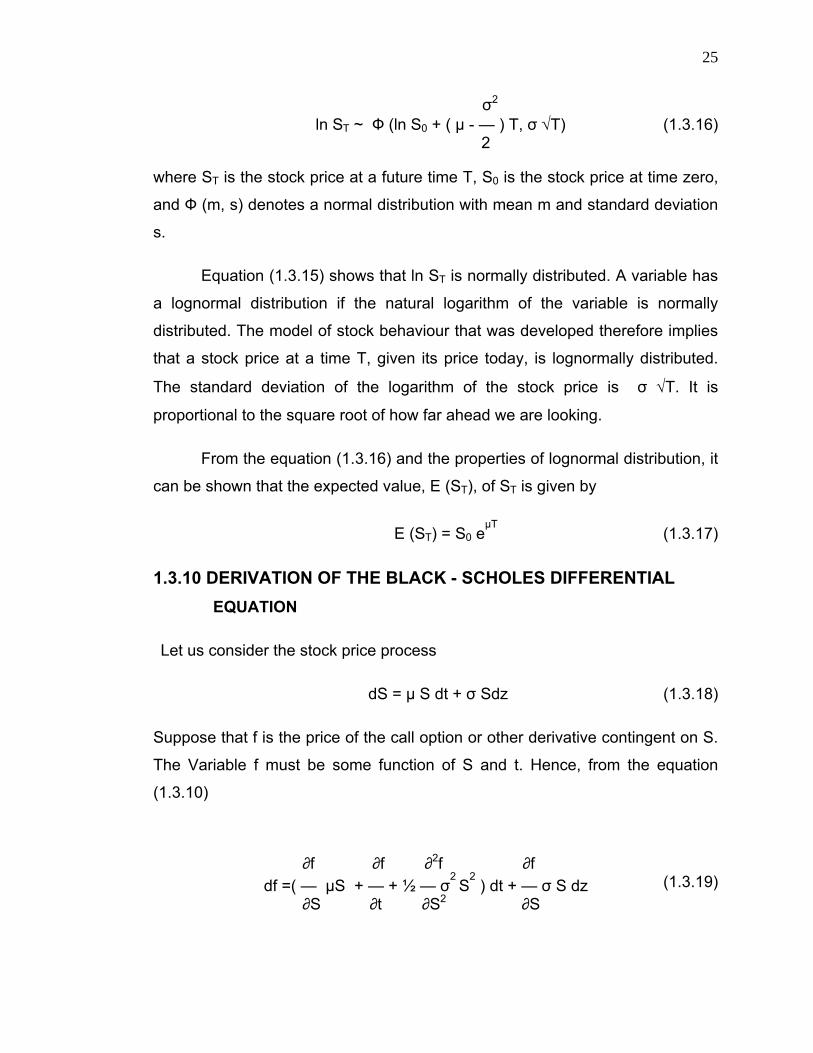
σ2

ln ST ~ Ф (ln S0 + ( µ - — ) T, σ √T) (1.3.16) 2

where ST is the stock price at a future time T, S0 is the stock price at time zero,

and Ф (m, s) denotes a normal distribution with mean m and standard deviation

s.

Equation (1.3.15) shows that ln ST is normally distributed. A variable has

a lognormal distribution if the natural logarithm of the variable is normally

distributed. The model of stock behaviour that was developed therefore implies

that a stock price at a time T, given its price today, is lognormally distributed.

The standard deviation of the logarithm of the stock price is σ √T. It is

proportional to the square root of how far ahead we are looking.

From the equation (1.3.16) and the properties of lognormal distribution, it

can be shown that the expected value, E (ST), of ST is given by

E (ST) = S0 eµT

(1.3.17)

1.3.10 DERIVATION OF THE BLACK - SCHOLES DIFFERENTIAL EQUATION

Let us consider the stock price process

dS = µ S dt + σ Sdz (1.3.18)

Suppose that f is the price of the call option or other derivative contingent on S.

The Variable f must be some function of S and t. Hence, from the equation

(1.3.10)

∂f ∂f ∂2f ∂f df =( — µS + — + ½ — σ

2 S2 ) dt + — σ S dz (1.3.19)

∂S ∂t ∂S2 ∂S

26

The discrete versions of the above equations are as below

δS = µ S δt + σ S δz (1.3.20)

∂f ∂f ∂2f ∂f

df =( — µS + — + ½ — σ2S2 ) δt + — σ S δz (1.3.21) ∂S ∂t ∂S2 ∂S

where, δS and δf are the changes in f and S in a small time interval δt.

From Itô’s lemma it is understood that the Wiener processes underlying f and S

are the same. In other words, the δz (=ε√δt) in equation (1.3.20) and (1.3.21)

are the same. It follows that, by choosing a portfolio of the stock and the

derivative, the Wiener process can be eliminated.

The appropriate portfolio is as follows:

- 1 — : derivatives

∂ f + — : shares ∂ S

The holder of the portfolio is short one derivative and long an amount ∂f/ ∂S of

shares. Define π as the value of the portfolio. By definition,

∂ f π = - f + — S (1.3.22)

∂S

The change in δ π in the value of the portfolio in the time interval δt is given by

∂ f δ π = - δf + — δS (1.3.23)

∂ S

Substituting equations (1.3.20) and (1.3.21) into equations (1.3.22) yields

∂f ∂2f δ π = (— - ½ — σ2 S2) δt (1.3.24)

∂t ∂S2

27

Because this equation does not involve δz, the portfolio must be riskless during

time δt. The assumptions listed in preceding section imply that the portfolio

must instantaneously earn the same rate of return as other short-term risk-free

securities. If it earned more than this return, arbitrageurs cold make a riskless

profit by borrowing money to buy the portfolio; if it earned less, they could make

a riskless portfolio by shorting the portfolio and buying risk-free securities. It

follows that

δ π = r π δt

where, r is the risk-free interest rate. Substituting from equation (1.3.22) and

(1.3.24), it becomes

∂f ∂2f ∂f ∂ (— - ½ — σ2 S2) δt = r (f - — S) δt

∂t ∂S2 ∂S so that

∂f ∂f ∂

2f

— + r S — + ½ σ2 S2 — = r f (1.3.25) ∂t ∂S ∂S2

Equation above is the Black – Scholes differential equation. It has many

solutions, corresponding to all the different derivatives that can be defined with

S as the underlying variable. The particular derivative that is obtained when the

equation is solved depends on the boundary conditions that are used. These

specify the values of the derivatives at the boundaries of possible values of S

and t. In the case of a European call option, the key boundary condition is

f = max (S - X, 0) when t = T

In the case of a European put option, it is

28

f = max (X - S, 0) when t = T

One point that should be emphasized about the portfolio used in the

derivation of equation (1.3.25) is that it is not permanently riskless. It is riskless

only for an infinitesimally short period of time. As S and t change, ∂f / ∂S also

changes. To keep the portfolio riskless, it is therefore necessary to frequently

change the relative proportions of the derivative and the stock in the portfolio.

1.3.10.1 The prices of tradable derivatives

Any function f(S, t) that is a solution of the differential equation (1.3.25) is

the theoretical price of a derivative that could be traded. If a derivative with that

price existed, it would not create an arbitrage opportunities. Conversely, if a

function f(S, t) does not satisfy the differential equation (1.3.25), it cannot be the

price of the derivative without creating arbitrage opportunities for the traders.

To illustrate this point, consider the function eS. This does not satisfy the

differential equation (1.3.25). It is therefore not a candidate for being the price of

a derivative dependent on the stock price. If an instrument whose price was

always eS existed, there would be an arbitrage opportunity.

Also consider the function e(σ2-2r)(T- t)

/ S. This does not satisfy the

differential equation, and so is, in theory, the price of a tradable security.

1.3.11 RISK – NEUTRAL VALUATION

Risk – neutral valuation is the single most important tool for analysis of

derivatives. It arises from one key property of the Black – Scholes differential

equation. This property is that the equation does not involve any variable that is

affected by the risk preference of the investors. The variables that do appear in

the equation are the stock price, time, stock price volatility, and risk-free rate of

interest. All are independent of risk preferences.

29

Black – Scholes differential equation would not be independent of risk

preferences if it involved the expected return on the stock µ. This is because the

value of µ does depend on risk preferences. The higher the level of risk

aversion by the investors, the higher µ will be for any given stock. It is fortunate

that µ happens to drop out in the derivation of the differential equation.

Because the Black – Scholes differential equation is independent of risk

preferences, an ingenious argument can be used. If risk preferences do not

enter the equation, they cannot affect its solution. Any set of risk preferences

can, therefore be used when evaluating f. In particular, the very simple

assumption that all investors are risk neutral can be made.

In a world where investors can be risk neutral, the expected return on all

securities is the risk-free rate of interest, r. The reason is that risk- neutral

investors do not require a premium to induce them to take risks. It is also true

that the present value of any cash flow in a risk neutral world would be obtained

by discounting its expected value at risk-free rate of interest. The assumption

that the world is risk neutral, therefore, considerably simplifies the analysis of

derivatives.

Consider a derivative that provides a payoff at one particular time. It can

be valued using risk - neutral valuation by using the following procedure:

1. Assume that the expected return from the underlying asset is the risk-

free rate of interest, r (i.e. assume µ = r).

2. Calculate the expected payoff from the options at its maturity.

3. Discount the expected payoff at the risk-free rate of interest.

It is important to appreciate the risk - neutral valuation (or assume that all

investors are risk - neutral) is merely an artificial device for obtaining solutions

to the Black – Scholes differential equation. The solutions that are obtained are

30

valid in all worlds, not just those were investors are risk – neutral. When we

move from risk - neutral world to a risk averse world, two things happen. They

are the expected growth rate in the stock price changes and the discount rate

that must be used for any payoffs from any derivative changes. It happens that

these two changes always offset each other exactly.

1.3.11.1 Application to Forward Contracts on a Stock

Assume that the interest rates are constant and equal to r. This is

somewhat restrictive. Consider a long forward contract that matures at time T

with delivery price X. The value of the contract at maturity is

ST – X

where ST is the stock price at time T. From the risk - neutral valuation argument,

the value of the forward contract at time zero is its expected value at time T

discounted at risk-free rate of interest. If we denote the value of the forward

contract at time zero by f, this means that

f = e-rT Ê(ST - X) (1.3.26)

where Ê is the expected value in a risk - neutral world. Because X is a constant,

equation (1.3.26) becomes

f = e-rT

Ê(ST ) – X e-rT

(1.3.27)

The expected growth rate of the stock price, µ, becomes r in a risk - neutral

world, which, can be expressed as:

Ê(ST ) = S0 erT (1.3.28)

Substituting equation (1.7.28) into equation (1.7.25) gives

f = S0 – X e-rT

(1.3.29)

31

1.3.12 BLACK – SCHOLES OPTION PRICING FORMULA

One way of deriving the Black - Scholes formula is by solving the

differential equation (1.7.25) subject to the boundary conditions explained in the

above section 1.7.9. Another approach is to use the risk - neutral valuation.

Consider a European call option. The expected value of the option at any

maturity in a risk - neutral world is

Ê [max (ST – X, 0)]

where Ê denotes the expected value in a risk - neutral world. From the risk -

neutral valuation argument, the European call option, c, is the expected value

discounted at the risk-free rate of interest, that is,

Co = e-rT

Ê [max (ST – X, 0)] (1.3.30)

Let us consider a call option on a non-dividend-paying stock maturing at time T.

Under the stochastic process assumed by Black – Scholes, ST is lognormal.

Also from the equation (1.3.16) and (1.3.17), Ê (ST) = S0 erT

and the standard deviation of ln S is σ √T.

Key result:

If V is lognormally distributed and the standard deviation of ln V is s, then

E [max (V-X), 0] = E (V) N (d1) – X N (d2) (1.3.31)

where

ln [E(V) / X] + s2 /2 d1 = ----------------------- (1.3.32)

s ln [E(V) / X] - s2 /2

d2 = ----------------------- (1.3.33) s

32

E denotes the expected value.

From the key result just proved, the equation (1.7.31) implies that

Co = e-rT

[S0erT

N (d1) – X N(d2)]

= S0 N(d1) – X e-rT

N(d2) (1.3.34)

where

ln [Ê(ST) / X) + σ2T /2]

d1 = ------------------------------- σ √T ln (S0 / X) + (r + σ

2 /2] T

d1 = ------------------------------- (1.3.35) σ √T ln [Ê(ST) / X) - σ

2T /2]

d2 = ------------------------------- σ √T ln (S0 / X) + (r - σ

2 /2] T

d2 = ------------------------------- (1.3.36) σ √T

= d1 - σ √T

1.4 STATEMENT OF THE PROBLEM

Buying decision depends upon the intrinsic (correct) value of the asset to

be purchased and the investor’s ability to estimate the same. If the market price

is more than the estimated intrinsic price, one should sell the asset, as the

market price will converge with the intrinsic value in due course. If the market

price is less than the intrinsic value, then one should buy the asset before it

rises as more and more investors will find that the asset is undervalued and buy

33

the same. There are many asset pricing models being practiced in capital

market like Dividend Discount Model (DDM), Relative Valuation Models, Capital

Asset Pricing Model (CAPM), Single factor model, Stephen Ross’s Arbitrage

Pricing Theory (APT) etc. Likewise in last two decades, option pricing has

witnessed an explosion of new models after the celebrated and Nobel Prize

won Black – Scholes (1973) European formula. Examples include (i) the

Stochastic – Interest – rate option models of Merton (1973) and Amin and

Jarrow (1992); (ii) the Jump – Diffusion / Pure Jump models of Bates (1991),

Madan and Chang (1996), and Merton (1976); (iii) the Constant - Elasticity – of

- Variance model of Cox and Ross (1976); (iv) the Markovian models of

Rubinstein (1994) and Aït – Sahalia and Lo (1996); (v) the Stochastic –

Volatility models of Heston (1993), Hull and White (1987a), Melino and Turnbull

(1990, 1995), Scott (1987), Stein and Stein (1991), and Wiggins (1987); (vi) the

Stochastic – Volatility and Stochastic – Interest – rates models of Amin and

Victor Ng (1993), Baily and Stulz (1989), Bakshi and Chen (1997a,b), and Scott

(1997). But most of them are not as parsimonious as Black - Scholes model

and have difficulties in practice. Till now, Black - Scholes is considered as

benchmark for option pricing.

As seen early, the Black - Scholes (BS) option pricing formula, won the

Nobel Prize for economics in 1997, revolutionized the capital market. So many

empirical studies were conducted on the BS formula in developed nations,

which interestingly revealed the strengths and weaknesses of it. As India

introduced exchange - traded options only in 2001, an elaborate empirical study

is required in the usage of BS formula in Indian stock option market. First, the

sensitivity of the call option price on change in the variables / parameters is to

be studied in detail. That is the relationships between the call option price and

its determinants like price of the underlying asset, Strike Price, Risk-free

Interest rate, volatility of the returns of the underlying asset, remaining life of the

option etc. are to be analyzed and understood. Second, the research study is

on the predictability of the model, and biases of the model towards the above

34

determinants are to be identified and taken care when use. Third, model’s

specification is to be tested for its correctness, using residual analysis. Fourth, it

is to understand that the assumptions of the model are real and practically

correct. Lastly, the empirical study can also focus on any weakness of the

model and to improve the same to improve the predictability of the model.

1.5 NEED FOR THE STUDY

Once the investor decided to cap the downside risk of his investment,

using options, the next question arises that what is the premium to be paid or

the price to be given to enjoy such a risk management tool. This price shall be

logical and correct to make a decision of buying or selling an option. The

question of pricing the asset can be done in any number of ways explained in

earlier paragraph 1.2. But the investor - friendly, parsimonious method of option

pricing is the Black - Scholes option pricing model. Universally this model is

used in all the leading option exchanges including the developed nations like

USA, UK, Japan and emerging nations like India, China etc.

If we keenly observe, the volume and the range of options offered by

NSE in India and the actual options that are traded, it is easily understood that

still the Indian investors are not familiar with the options. At random, samples of

30 companies were taken which are given in Table no.1.1.

35

TABLE 1.1

DETAILS OF THE STOCK CALL OPTIONS OFFERED, TRADED AND NON - DIVIDEND PAYING STOCKS AT NSE FROM 1.1.02 TO 31.10.07

S. No.

1

Company

2

From

3

To

4

Offered

5

Traded

6

Non- Dividend Paying

7

1 Tata Steel 01/01/02 31/10/07 59,912 18,462 16,1002 Reliance Ind. 01/01/02 31/10/07 53,118 16,271 14,1453 Infosys 31/01/03 31/10/07 60,653 18,046 12,5594 ACC 01/01/02 31/10/07 56,006 11,577 9,3345 MTNL 01/01/02 31/10/07 49,049 13,085 9,2986 Satyam 01/01/02 31/10/07 53,376 16,122 8,6737 HUL 01/01/02 31/10/07 49,742 12,444 7,7768 Ranbaxy 01/01/02 31/10/07 57,502 9,975 7,4819 ITC 01/01/02 31/10/07 50,349 8,864 7,264

10 M & M 01/01/02 31/10/07 56,020 8,739 7,23211 Maruti 09/07/03 31/10/07 46,591 8,599 7,15712 Ambuja Cements 01/01/02 31/10/07 47,152 7,643 6,79313 ICICI 31/01/03 31/10/07 47,754 7,989 6,47514 ONGC 31/01/03 31/10/07 48,223 9,567 5,97815 SCI 31/01/03 31/10/07 45,178 6,962 5,57416 Hindalco 01/01/02 31/10/07 56,464 6,114 5,35317 BPCL 01/01/02 31/10/07 53,954 7,780 5,34718 Cipla 01/01/02 31/10/07 56,632 5,665 4,83319 Dr. Reddy'S 01/01/02 31/10/07 55,490 5,805 4,72120 Bank Of India 29/08/03 31/10/07 40,364 6,203 4,66021 Andhra Bank 29/08/03 31/10/07 33,559 5,896 4,51822 Wipro Ltd. 31/01/03 31/10/07 47,780 6,417 4,50523 Syndicate Bank 26/09/03 31/10/07 32,941 5,759 4,38924 UBI 29/08/03 31/10/07 36,327 5,166 4,12225 BHEL 01/01/02 31/10/07 65,471 6,051 4,08326 PNB 29/08/03 31/10/07 49,229 4,661 3,87027 Bank Of Baroda 29/08/03 31/10/07 49,764 4,457 3,58928 Canara Bank 29/08/03 31/10/07 46,500 4,676 3,26229 Bajaj Auto 01/01/02 31/10/07 63,292 2,331 1,79030 Grasim 01/01/02 31/10/07 64,195 2,086 1,761

Total 15,32,58 2,53,412 1,92,642Source: Column 1 to 6 from www.nseindia.com Note: The details for non-dividend paying stock are explained in paragraph 2.2.3.5 under research methodology

36

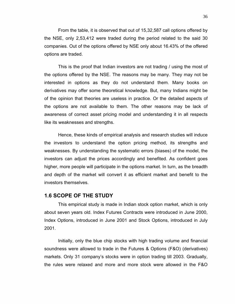
From the table, it is observed that out of 15,32,587 call options offered by

the NSE, only 2,53,412 were traded during the period related to the said 30

companies. Out of the options offered by NSE only about 16.43% of the offered

options are traded.

This is the proof that Indian investors are not trading / using the most of

the options offered by the NSE. The reasons may be many. They may not be

interested in options as they do not understand them. Many books on

derivatives may offer some theoretical knowledge. But, many Indians might be

of the opinion that theories are useless in practice. Or the detailed aspects of

the options are not available to them. The other reasons may be lack of

awareness of correct asset pricing model and understanding it in all respects

like its weaknesses and strengths.

Hence, these kinds of empirical analysis and research studies will induce

the investors to understand the option pricing method, its strengths and

weaknesses. By understanding the systematic errors (biases) of the model, the

investors can adjust the prices accordingly and benefited. As confident goes

higher, more people will participate in the options market. In turn, as the breadth

and depth of the market will convert it as efficient market and benefit to the

investors themselves.

1.6 SCOPE OF THE STUDY This empirical study is made in Indian stock option market, which is only

about seven years old. Index Futures Contracts were introduced in June 2000,

Index Options, introduced in June 2001 and Stock Options, introduced in July

2001.

Initially, only the blue chip stocks with high trading volume and financial

soundness were allowed to trade in the Futures & Options (F&O) (derivatives)

markets. Only 31 company’s stocks were in option trading till 2003. Gradually,

the rules were relaxed and more and more stock were allowed in the F&O

37

sections. In 2007, about 223 company’s stocks were included in option trading.

This study is made on those stocks options which are traded at least from

January 2002 to October 2007. Both National Stock Exchange and Bombay

Stock Exchange are trading stock options, but, the volume of the National Stock

Exchange is more than 98% of the total traded value and volume in India and

hence the study is confined to the options traded at National Stock Exchange

(NSE). More details are given in under research methodology, in the chapter II.

The options are offered in Stock market Index such as Nifty, the stocks, etc.

This study is restricted to the stock options that too call options only, as the BS

model itself is basically designed for call options.

1.7 OBJECTIVES OF THE STUDY

1.7.1 TESTS FOR THE BLACK-SCHOLES MODEL

Assessments of a model's validity can be done in two ways. First, the

model's predictions can be confronted with historical data to determine whether

the predictions are accurate, within some statistical standard of confidence.

Second, the assumptions made in developing the model can be assessed to

determine if they are consistent with observed behavior or historical data.

A long tradition in economics focuses on the first type of tests, arguing

that "the proof is in the pudding". It is argued that any theory requires

assumptions that might be judged "unrealistic", and that if we focus on the

assumptions, we can end up with no foundations for deriving the

generalizations that make theories useful. The only proper test of a theory lies

in its predictive ability: The theory that consistently predicts best is the best

theory, regardless of the assumptions required to generate the theory.

38

Tests based on assumptions are justified by the principle of "garbage in-

garbage out." This approach argues that no theory derived from invalid

assumptions can be valid. Even if it appears to have predictive abilities, those

can slip away quickly when changes in the environment make the invalid

assumptions more pivotal.

Our analysis takes an agnostic position on this methodological debate,

looking at both predictions and assumptions of the Black-Scholes model.

The main objective of this research is to make an empirical study of

Black - Scholes option pricing model in Indian stock call - option market and to

find an improvement in the model for better prediction ability, if possible.

The sub objectives are

i) To measure the sensitivity of the model in respect of each factors of

option pricing such as Stock Price, Strike Price, Time to Maturity,

Volatility of stock returns, and Risk – Free Rate of Interest.

ii) To analyze the predictability and the biases of the model, if any,

towards volatility, Time to maturity, Moneyness, risk free rate of

interest etc.

iii) To verify the model’s specification by analyzing the residuals of the

model, such as distribution of the residuals, mean, median, and

momentum analysis, correlation of residuals with the factors of

option price, etc.

iv) To analyze the validity of the model assumptions such as

lognormal returns of stocks, random walk of the stock price etc.

v) To find an improvement in the theoretical or practical part of the

model so that its prediction ability improves at least 5 to 10 percent.

39

1.8 REVIEW OF LITERATURE – RESEARCH STUDIES

There are many studies about the Black - Scholes model, the most

important studies published in the Journal of Finance, Number one Finance

journal in the world, are studied in depth and the findings are listed below.

The authors Black, Fisher, and Scholes ,Myron,[24] themselves admitted

some biases of the model in their research paper, “The Valuation of Option

Contracts and a Test of Market Efficiency”, expressed as “Using the past data

to estimate the variance caused the model to overprice options on high

variance stocks and underprice options on low variance stocks. While the

model tends to overestimate the value of an option on a high variance security,

market tends to underestimate the value, and similarly while the model tends to

underestimate the value of an option on a low variance security, market tends

to overestimate the value”.

During 1979, Macbeth, James D., and Merville, Larry J.[92] in their

research paper, “An Empirical Examination of the Black - Scholes Call Option

pricing Model” revealed that B-S model predicted prices are on average less

(greater) than market prices for in the money options (out of the Money) and

also had biases over the life of the options also. This study has some

coincidences and differences with the above findings which are also explained

in this chapter.

LIU, JINLIN [86], while researching the topic, “An Empirical Investigation

of Option Bounds Method”, opined that the BS formula worked better as a

whole than the Option Bounds Method. This phenomenon is interesting

because although one key assumption of BS’ is untrue, BS still works well for

real data of options. One possible explanation is that too many participants in

the market are using BS formula to price the options. Even when BS cannot

work well in reality, they apply something as OAS to modify the results.

40

However, the modifiers are still are based on the BS method. Consequently, the

BS method would fit the price in the market well.

Fortune, Peter , in his series of Federal Reserve Bank of Boston studies

titled “Anomalies in option pricing: the Black-Scholes model revisited” published

in New England Economic Review, March-April, 1996 [53], had concluded that

“the combined results suggest a 10 to 100 percent error for calls”. He also

added “In summary, the probability distribution of the change in the logarithm of

the S&P 500 does not conform strictly to the normality assumption. Not only is

the distribution thicker in the middle than the normal distribution, but it also

shows more large changes (either up or down) than the normal distribution.

Furthermore, the distribution seems to have shifted over time. After the Crash

an increase in the kurtosis and a shift in skewness occurred”

Ball, Clifford A. and Torous, Walter N. [13] during their study, "On Jumps

in Common Stock Prices and Their Impact on Call Option Pricing," compared

between Merton’s Jump- diffusion model and the Black - Scholes model. They

observed that there were no operationally significant differences in the models.

Empirical evidences confirm the systematic mispricing of the Black -

Scholes call option pricing Model. These biases have been documented with

respect to the call option’s exercise price, its time to expiration, and the

underlying common stock’s volatility. Black [24] reports that the model over

prices the deep in-the-money options, while it underprices deep out-the-money

options. By contrast, Macbeth, James D. and Merville, Larry J. [92] state that

deep in-the-money options have model prices that are lower than the market

prices, whereas, deep out -the-money options have model prices that are

higher. These conflicting results may perhaps be reconciled by the fact that the

studies examined market prices at different point in time and these systematic

errors vary with time (Rubinston [111]).

41

A number of explanations for the systematic price bias have been

suggested (Geske and Roll [57]). Among these is the fact that Black - Scholes

assumptions of lognormally distributed security price fails to systematically

capture the important characteristics of the actual security price process.

1.9 LIMITATIONS OF THE STUDY

The study is limited to National Stock Exchange and limited to stock

options, which are traded from January 2002 till October 2007 as the trades in

BSE has been less than one percentage compare to NSE trade. The risk-free

rates are obtained from the Mumbai Inter-Bank Offer rates (MIBOR) and

Mumbai Inter-Bank Bid Rates (MIBID) as taken by the NSE itself. The foreign

countries are using T - Bill rates as risk-free rates. But in India the T-bill market

is not matured and deep and hence the MIBOR / MIBID are taken as a proxy for

the risk – free rates. NSE is also using the same. The study is limited to call

options only as the BS model is basically derived for call options.

1.10 CHAPTER PLAN

The first chapter represents a brief history of options, its growth and its

importance in International and Indian derivative Markets. Further it includes

statement of the problem, objectives, basics of options, factors influencing

options, pricing methods, basics and derivation of Black – Scholes formula and

its assumptions. An overview of earlier studies, the empirical studies in the

foreign nations and its findings are included. A brief notes on the individual

journal papers relevant to our study and their findings are narrated. It ends with

the limitations of the research.

42

The second chapter deals with a brief research methodology applied for

the empirical verification, including the statistical tools used / procedures. It also

narrates the data collection, culling out the traded data from the offered options,

method of removing the risk-free arbitrage opportunities, exclusion of data

related to ex-dividend dates within the option life and finalization of data for

analysis.

In chapter three, each of the five factors is taken separately and studied

in depth about the sensitivity of the price of option by changing the variables

and parameters step by step. The price of the option is more sensitive to some

of the factors than others. Full examination details are given in this chapter.

Fourth chapter explains the model’s prediction ability and pattern of the

option pricing calculated using BS formula, towards its determinants like

volatility of returns of the stock, exercise price, moneyness of the option, risk –

free rate, life of the option etc. The findings of the study are explained in depth.

Partial study with the data up to 30.6.2004 on biases of the model had been

published in the Book titled “Business Management Practices, Policies and

Principles” by The Allied Publishers Private Limited, New Delhi, after editing by

faculty of Indian Institute of Management, Indore [105] (Annexure I).

In the Fifth chapter, residual analysis being one of the important tools of

modern econometrics is used to analyze the model adequacy; the interesting

findings are explained in length and breadth in this chapter. This study

“Residual Analysis of the Model” was presented in the National Conference on

Business Research conducted by P.S.G. Institute of Management and won the

Best Paper Award in finance session and the same was published in the

Journal of Management Research Volatility.1, No.2, April - June 2006, [106]

(Annexure II).

Sixth chapter deals with the BS model assumptions while developing the

model and examines the validity of these seven important assumptions in

43

practice. The empirical verification of one of the main assumptions of the model

that the stock price follows a random walk itself is vast and equals to a mini

research in technical analysis. The fascinating empirical findings are narrated in

depth in this chapter.

Chapter seven reveals the efforts made to improve the BS model’s

predictability and the logic behind the selection of the variables / parameter for

improvement. The number of improvements effected and the percentage of

improvement achieved due to the envisaged new method are enlightened in

depth.

Chapter eight deals with the fulfillment with the objectives of the study

considered. The findings emerged out of this empirical study is enumerated and

suggestions of the researcher are given to the investors and academicians and

the conclusion. The scopes of further research and recommendations for further

research are added towards the end.