68 CHAPTER FOUR TECHNICAL EFFICIENCY OF ETHIOPIAN MICROFINANCE INSTITUTIONS 4.1 Introduction This chapter aims to measure the technical efficiency and its determinants of the MFIs. Methodologically, efficiency of the MFIs is estimated using the preferred DEA and then complimented the SFA for the robustness of the results. The remaining part of this chapter is structured as follows. Content wise, the chapter begins with discussion of prior empirical finding on efficiency of MFIs in the globe. The next section provides the methodology i.e., the DEA model specification, and input and output selection. Then section three presents results and discussions. Finally, section four presents the conclusion. 4.2 Prior empirical works on efficiency of MFIs Though the efficiency of the banking sector is adequately examined, researches related to the efficiency of MFIs in general are limited. This fact is substantiated by Berger and Humphrey (1997). Their survey shows that more than 130 studies have used the frontier techniques in analyzing efficiency of banks in different countries. On the other hand, a survey by Cummins and Weiss (2000), which focuses on efficiency in the insurance industry, has found 21 studies which applied frontier techniques. A more recent survey

Welcome message from author
This document is posted to help you gain knowledge. Please leave a comment to let me know what you think about it! Share it to your friends and learn new things together.
Transcript

68
CHAPTER FOUR
TECHNICAL EFFICIENCY OF ETHIOPIAN
MICROFINANCE INSTITUTIONS
4.1 Introduction
This chapter aims to measure the technical efficiency and its determinants of the MFIs.
Methodologically, efficiency of the MFIs is estimated using the preferred DEA and then
complimented the SFA for the robustness of the results. The remaining part of this
chapter is structured as follows. Content wise, the chapter begins with discussion of prior
empirical finding on efficiency of MFIs in the globe. The next section provides the
methodology i.e., the DEA model specification, and input and output selection. Then
section three presents results and discussions. Finally, section four presents the
conclusion.
4.2 Prior empirical works on efficiency of MFIs
Though the efficiency of the banking sector is adequately examined, researches related to
the efficiency of MFIs in general are limited. This fact is substantiated by Berger and
Humphrey (1997). Their survey shows that more than 130 studies have used the frontier
techniques in analyzing efficiency of banks in different countries. On the other hand, a
survey by Cummins and Weiss (2000), which focuses on efficiency in the insurance
industry, has found 21 studies which applied frontier techniques. A more recent survey

69
by Luhen (2009) found more than 93 studies using frontier efficiency measurement with
application to the insurance industry. However, only studies of (Nghiem,2004; Gutierrez-
Nieto et al., 2005; Gutierrez-Nieto et al., 2009; Hassan and Tuffe, 2001; Qayyum and
Ahmed, 2006; Haq et al., 2007; Sufian, 2006; Bassem, 2008; Hermes et al., 2009; Hassan
and Benito, 2009; Nawaz, 2009; Masood and Ahmed, 2010,Oteng-Abayie et al., 2011)
are found in microfinance institutions. The findings of these empirical studies are
thoroughly discussed below.
Guitierrez-Nieto et al. (2005) applied a DEA non-parametric approach to analyze the
efficiency of 30 Latin American MFIs. In their study, they tried to explore the
multivariate analysis of the DEA results by developing 21 specifications using two inputs
and three outputs. Their study found that an NGO and a non-bank financial institution are
the most efficient among the various group of MFIs.
Bassem (2008) estimated efficiency of 35 microfinance institutions in the Mediterranean
zone during the period 2004–2005 using DEA and found that eight institutions were
efficient. Further, the study revealed that size of the MFI has a negative effect on
efficiency.
Hassan and Sanchez (2009) applied DEA to investigate the technical and scale
efficiencies of microfinance institutions (MFIs) in three regions: Latin America countries,
Middle East and North Africa (MENA) countries, and South Asia countries, and
compares efficiencies across regions and across type of MFIs. They found that technical
efficiency is higher for formal MFIs (banks and credit unions) than non-formal MFIs
(nonprofit organizations and non-financial institutions). Furthermore, South Asian MFIs

70
have higher technical efficiency than Latin American and MENA MFIs. Finally they
concluded that the source of inefficiency was pure technical rather than scale, suggesting
that MFIs were either wasting resources or were not producing enough outputs (making
enough loans, raising funds, and getting more borrowers).
Masood and Ahmed (2010) applied a stochastic frontier model to estimate the efficiency
of 40 Indian microfinance institutions for the period 2005-2008. They found that mean
efficiency level of microfinance institutions is low (34%) but it increases over the period
of study. The study also estimated determinants of efficiency and the result showed that
age of microfinance institution is positive determinant of efficiency. Further, the study
found regulated microfinance institutions are less efficient.
Haq et al. (2009) investigates the efficiency of 39 MFIs in developing world (Africa,
Asia, and Latin America) using the data envelopment analysis (DEA) based
intermediation and production approaches. These diffident approaches tend to give them
conflicting results. Their findings show that non-governmental microfinance institutions
under production approach are the most efficient. On the other hand, the study shows
bank-microfinance institutions outperform and are more efficient under intermediation
approach.
Servin et al. (2012) using stochastic frontier analysis examines technical efficiency of
different types of microfinance institutions in Latin America. Their sample includes 315
MFIs operating in 18 Latin American countries for the period 2003-2009. Their
methodology permits them both the production frontier and error structures to differ
between four types of ownership types of MFIs (NGO, Cooperative/Credit Union, Non-

71
Bank Financial Intermediary and Bank). They differentiate between intra-firm and inter-
firm efficiency. Their results show that Non-Governmental Organizations and
Cooperatives/Credit Unions have much lower inter-firm and intra-firm technical
efficiencies than Non-Bank Financial Intermediaries and Banks, which indicates the
importance of ownership type for technical efficiency. According to the authors, the
finding that NGOs and Cooperative/Credit Unions now are, on average, less efficient
than mutual NBFIs and Banks seem to suggest that further increases in regulation and
competition will be needed to curtailing inefficiencies of non-share holder MFIs.
Abdul Qayyum and Ahmad (2006) tried to investigate the efficiency of 85 MFIs in South
Asia (consisting of 15 Pakistani, 25 Indian, and 45 Bangladeshi). The analysis revealed
that the inefficiency of the MFIs in Pakistan, India, and Bangladesh is mainly of technical
nature and to improve their efficiencies, they suggest that the MFIs need to enhance their
managerial expertise and improve technology.
Nghiem et al. (2004) investigates the efficiency of microfinance industry in Vietnam
through a survey of 46 schemes in the north and central regions by employing the Data
Envelopment Analysis (DEA). The result of the study reveals that the average technical
efficiency score of schemes is 80%. Further, the study found that age and location have
positive effect on efficiency of the schemes.
Hassan and Tufte (2001) examine cost inefficiency and determinants of the Grameen
Bank (GB) using branch level cost data over the 1988-1991 period. Using a stochastic
frontier analysis they found that Grameen Bank’s branches staffed by the female

72
employees operated more efficiently than their counterparts staffed by the male
employees.
Gregorio and Ramirez (2004) analyzed the efficiency of Microfinance Institutions (MFIs)
in Peru between 1999 and 2003 by estimating a stochastic cost frontier. They found
that MFIs with the largest assets tend to post the highest efficiency levels and
that MFIs operating in less concentrated market tend to be more efficient. Further their
study shows that cost efficiency of MFIs is affected by average loan size, proportion of
net assets, financial sufficiency, financial leverage, business experience and proportion of
farm loans.
Sufian (2006) also analyzed the efficiency of 80 Non Bank Financial Institutions (NBFI)
in Malaysia for the period 2000–2004 using DEA. His study revealed that only 28.75% of
80 observations are efficient. Moreover, his study revealed that the size and the part of
the market have a negative effect on efficiency.
Martinez-Gonzalez (2008) examined the relative technical efficiency of a sample of
microfinance institutions (MFIs) in Mexico using the data envelopment analysis (DEA).
The study found that most of the MFIs have been more successful in achieving the type
of efficiency related to sustainability rather than outreach. Further the study found that
average size of loan, proportion of assets used as performing portfolio, percentage of
FINAFIM funds, scale of operations, ratio of payroll to expenses, age, structure of
the board, and for-profit status of the MFI have significant impact on efficiency of
MFIs.

73
Hermes et al. (2008) used stochastic frontier analysis to examine a trade-off between
outreach to the poor and efficiency of microfinance institutions based on 435 MFIs and
found that outreach and efficiency of MFIs are negatively correlated. Their finding
further indicates that efficiency of MFIs is higher if they focus less on the poor and/or
reduce the percentage of female borrowers.
Nawaz (2010) attempts to measure the financial efficiency and productivity of
Microfinance Institutions (MFIs) worldwide taking into account the subsidies received by
MFIs by using the non-parametric Data Envelopment Analysis (DEA). The study carried
out a three-stage analysis. Firstly, technical and pure efficiency scores are calculated by
splitting subsidies into input and output and entered into the DEA framework
specifications depending on whether they are generating benefits (negative subsidies) or
cost (positive subsidies) to the society. Secondly DEA-based Malmquist indices are
calculated to analyze the intertemporal productivity change. Thirdly, Tobit Regression
analysis are carried out to test a series of hypotheses concerning the relationship between
financial efficiency and other indicators related to MFIs productivity, organization,
outreach, sustainability and social impact. The study concludes that overall subsidies
contribute to financial efficiency of MFIs albeit marginally. The study also provides
evidence on the tradeoff between outreach to the poor and financial efficiency. That is
MFIs which cater to the poor tend to be more inefficient than those with clients relatively
well off. Also evident is the fact that lending to women is efficient only in the presence of
subsidies MFIs in South Asia and Middle East & North Africa tend to be less efficient
than the others.

74
Ahmad (2011) has attempted to estimate the efficiency of microfinance institutions in
Pakistan. The non parametric Data Envelopment Analysis has been used to analyze the
efficiency of these institutions by using data for the year 2003 and 2009 respectively.
Both input oriented and output oriented methods have been considered under the
assumption of constant return to scale and variable returns to scale. He found that three
MFIs are on efficiency frontier in the year 2003 under both constant return to scale and
variable return to scale assumptions. Further, in year 2009, four microfinance institutions
are efficient under constant return to scale and nine are efficient under variable return to
scale assumption.
Oteng-Abayie et al. (2011) estimates economic efficiency of 137 microfinance units in
Ghana for 2007-2010 sample periods using a Cobb-Douglas stochastic frontier model.
They found that the MFIs are producing at constant cost to size with an overall average
economic efficiency for the group of MFIs to be 56.29%. Further their study reveals that
the main sources of inefficiencies in the microfinance sector in Ghana are due to the
variation in management practices and differences in technical capacities (both in training
and portfolio quality). Finally, the study reveals that age and savings indicators of
outreach and productivity, and cost per borrower are found to be significant determinants
of economic efficiency.

75
Source: Author’s survey
Table 4.1: Efficiency studies on MFIs
Author Data description Approach
Hassan and Sanchez(2009) 215 MFIs in the world DEA
Gutierrez-Nieto et al. (2007) 21 MFIs in Latin America DEA
Hamiza Haq et al. (2007) 39 MFIs from the world DEA
Abdul Qayyum and Munir Ahmed (2006) 85 MFIs from India, Pakistan and Bangladesh DEA
Nghiem (2004) 46 MFIs in Vietnam DEA and SFA
Ahmed Nawaz (2009) 204 MFIs around the world DEA
Bassem(2008) 35 MFIs in Mediterranean DEA
Hassan and Tufte (2001) Grameen Bank branch level over the 1988-1991 period SFA
Hermes et al. (2009) 435 MFIs in the world for the period 1997-2007 SFA
Oteng-Abayie et al. (2011) Ghana MFIs for the period from 2007-2010 SFA
Masood and Ahmed (2010) 40 Indian microfinance institutions for the period 2005-2008 SFA
Gregorio and Ramirez (2004) Peru MFIs for the period of 1999-2003 SFA
Martinez-Gonzalez (2008) Sample MFIs in Mexico DEA
Ahmed (2011) MFIs in Pakistan DEA
Servin et al. (2012) 315 MFIs from Latin America SFA

76
4.3 Methodology
In empirical works on the efficiency of financial institutions the parametric - SFA and the
non parametric – DEA are overwhelmingly dominating (Berger and Humphrey, 1997).
The DEA involves the use of linear programming whereas SFA involves the use of
econometric methods (Coelli et al., 1998). As the SFA impose functional and
distributional forms on the error term, the DEA does not require any functional form to
be specified. Further, while the former distinguishes the component of inefficiency in to
random and inefficiency effect, the later deems any deviation from the efficiency frontier
to the result of inefficiency. Studies acknowledged that both approaches have advantages
as well as limitations (Berger and Humphrey, 1997).The superiority of one approach over
the other has been a discussion and is still debatable in literature of financial institutions.
However, still others suggest that, for instance, Resti (1997); Ondrich and
Ruggiero(2000); and Leon(2001) both produce similar rankings, and conclude that both
approaches are complimentary to measure efficiency. Indeed, the nonparametric DEA is
more frequently used than parametric methods (Berger and Humphrey, 1997).
Parametric measurement includes specifying and estimating a stochastic production
frontier or stochastic cost frontier. In this method, the output (or cost) is assumed to be
function of inputs, inefficiency and random error. The main strength of the stochastic
frontier function approach (SFA) is its incorporation of stochastic error, and therefore
permitting hypothetical testing. An often quoted disadvantage of this approach, however,
is that it imposes an explicit functional form and distribution assumption on the data.

77
In contrast, the linear programming technique of data envelopment analysis (DEA) does
not impose any assumptions about functional form; hence it is less prone to mis-
specification. Further, DEA is a non-parametric approach so does not take into account
random error. Hence, it is subject to the problems of assuming an underlying distribution
about the error term. However, since DEA cannot take account of such statistical noise,
the efficiency estimates may be biased if the production process is largely characterized
by stochastic elements.
For the purpose of this study the non parametric DEA is preferred at least for three
reasons. First it considers multiple inputs and multiple outputs to assess the efficiency of
MFIs (i.e the dual objectives of social and financial).Second it does not require a prior
assumption about the analytical form of the production function. Third, DEA works well
with small number of observations as the case of Ethiopian MFIs.
4.3.1 Data envelopment analysis (DEA)
Originally, DEA was first introduced in the work of Farrell (1957) and then developed in
the work of Charnes et al. (1978) and is applied to non-profit organizations where the
objective of profit maximization and cost minimization may not be considered as the vital
factor. It has been extensively applied in performance evaluation and benchmarking of
schools, hospitals, bank branches, production plants, financial institutions (Charnes et al.,
1994; and Berger and Humphrey, 1997).
The DEA technique is essentially a linear programming technique that converts multiple
inputs and outputs into a measurement of efficiency. This conversion is conducted by

78
analyzing the resources (inputs) used and the results (outputs) achieved for each decision
making unit (DMU) or microfinance institution. The inputs and outputs of each DMU
(microfinance institution) are compared to the same quantities for all the remaining units.
The DEA identifies the most efficient units in a population and provides a measurement
of inefficiency for all the others. The method constructs a frontier based on actual data.
Firms on the frontier are efficient, while firms off the efficiency frontier are
inefficient.DEA is based on the concept of relative efficiency and is widely used in
efficiency and productivity analysis of financial institutions (see, Berger and Murphy,
1997). Moreover, DEA provides information about peers, which are the efficient schemes
that have similar input-output structure as some inefficient schemes.
In DEA, efficiency can be measured by an input-oriented process, which focuses on
reducing inputs to produce the same level of outputs, and an output-oriented process,
which aims to maximize outputs from a given set of inputs. The two measures provide
the same results under constant returns to scale but give different values under variable
returns to scale (Fare and Lovell 1978; Coeli et al., 1998). Furthermore, the choice of an
orientation will have only minor influences upon efficiency scores (Coelli et al., 1998).
However, this study is based on output oriented DEA which assumes the optimal output
that can be produced given a set of inputs. The output orientation seems more appropriate
to MFIs because such institutions are expected to reach many discriminated poor people
using a given level of inputs.
The DEA technical efficiency is calculated by assuming both Constant Returns to Scale
(CRS) and Variable Returns to Scale (VRS). The CRS assumption is only appropriate

79
when all DMUs are operating at an optimal scale. However, factors like imperfect
competition and constraints on finance may cause a DMU not to operate at optimal scale
(Coelli et al., 1996). Banker, Charnes and Cooper (1984) suggested an extension of the
CRS DEA model to account for variable returns to scale. The use of the CRS
specification when not all DMU’s are operating at the optimal scale will result in measure
of technical efficiencies which are confounded by scale efficiencies. The use of the VRS
specification will permit the calculation of pure technical efficiency devoid of these scale
efficiency effects. This study assumes the variable return to scale as it seems appropriate
for MFIs particularly operating in developing countries such as Ethiopia. However, for
comparison both assumptions are pursued to estimate the efficiency of the MFIs. By
running both CRS and VRS it is possible to decompose technical efficiency into pure
technical efficiency and scale efficiency and therefore to determine whether a DMU has
been operating at optimal returns to scale, increasing returns to scale, or decreasing
returns to scale ( Celli, 1996).
The study is based on Charnes, Cooper and Rhodes (1978) - CCR model and Banker,
Charnes and Cooper (1984)- BCC model. The basic difference between these two models
is the treatment of returns to scale. While the latter takes into account the effect of
variable returns to scale (VRS), the former restricts DMUs to operate with constant
returns to scale (CRS).
Assume that there are n Decision Making Units (DMUs), and each DMU has m inputs to
produce s outputs. This model measures the relative efficiency ratio of a given DMU (ho)

80
by the sum of its weighted outputs to the sum of its weighted inputs. It can be formulated
as follows as follows:
Max ho=∑ 𝑢𝑟 𝑦𝑟𝑜𝑠𝑟=1∑ 𝑣𝑖 𝑚𝑖=1 𝑥𝑖𝑜
Subject to
∑ 𝑢𝑟 𝑠𝑟=1 𝑦𝑟𝑗
∑ 𝑣𝑖𝑚𝑖=1 𝑥𝑖𝑗
≤ 1, (4.1)
𝑢𝑟 𝑣𝑖 ≥ 0, 𝑖 = 1, … ,𝑚, 𝑗 = 1, … ,𝑛, 𝑟 = 1, … , 𝑠,
where ℎ𝑜is the efficiency ratio of the DMU𝑜;𝑢𝑖 ,𝑢𝑟are virtual multipliers (weights) for the
i th input and the r th output, respectively; m is the number of inputs, s is the number of
outputs and n is the number of DMUs; 𝑥𝑖𝑜is the value of the input i for DMUo, 𝑦𝑟𝑜is the
value of the output r for DMUo.
The equation (1) is fractional programming and has an infinite number of solutions. It can
be solved by adding an additional constraint, ∑ 𝑣𝑖 𝑚𝑖=1 𝑥𝑖𝑜 = 1 . The form then converts to
the multiplier form of the DEA LP problem:
Maxℎ𝑜 = � 𝜇𝑟 𝑦𝑟𝑜𝑠
𝑟=1 (4.2)
Subject to
� 𝜇𝑟 𝑦𝑟𝑜 −� 𝑣𝑖 𝑥𝑖𝑗𝑚
𝑖=1
𝑠
𝑟=1≤ 0, 𝑗 = 1, … ,𝑛,

81
To reflect the transformation, the variables from (u, v) have been replaced by (μ, ν). ε is a
non‐Archimedean quantity defined to be smaller than any positive real number. The dual
form of equation (2) can be written as an equivalent envelopment form as follows:
minℎ𝑜 = 𝜃𝑜 − 𝜀(� 𝑠𝑖− + � 𝑠𝑖+𝑠
𝑟=1
𝑚
𝑖=1)
Subject to
� 𝑥𝑖𝑗
𝑛
𝑗=1𝜆𝑗 + 𝑠𝑖− = 𝜃𝑥𝑖𝑜, 𝑖
= 1, … ,𝑚, (4.3)
� 𝑦𝑟𝑗𝑛
𝑗=1𝜆𝑗 − 𝑠𝑟+ = 𝑦𝑟𝑜, 𝑟 = 1, …,
𝜆𝑗 ,𝑠𝑖−, 𝑠𝑟+ ≥ 0, 𝜀 > 0, 𝑗 = 1, … ,𝑛,
Where 𝜃𝑜 the proportion of DMUo′s inputs needed to produce a quantity of outputs
equivalent to its benchmarked DMUs identified and weighted by the𝜆𝑗 . 𝑠𝑖−. and 𝑠𝑟+are the
slack variables of input and output respectively. 𝜆𝑗is a (𝑛 × 1)column vector of constants
and can indicate benchmarked DMUs of DMUo. If ℎ0∗ = 1 is meant efficient and ℎ𝑜∗ < 1
is meant inefficient where the symbol “*” represents the optimal value.
However, the CCR model is calculated with the constant returns to scale (CRS)
assumption. This assumption is not supportable in imperfectly competitive markets. The
BCC model proposed by Banker, Charnes and Cooper (1984) modifies the CCR model

82
by allowing variable returns to scale (VRS). The CRS LP problem can be easily modified
to account for VRS by adding the convexity constraint
∑ 𝜆𝑗𝑛𝑗=1 = 1 to equation 4.3 to provide
minℎ𝑜 = 𝜃𝑜 − 𝜀(� 𝑠𝑖−𝑚
𝑖=1+ � 𝑠𝑟+
𝑠
𝑟=1)
Subject to
� 𝑥𝑖𝑗𝑛
𝑗=1𝜆𝑗 + 𝑠𝑖− = 𝜃𝑥𝑖𝑜, 𝑖 = 1, … ,𝑚, (4.4)
�𝑦𝑟𝑗
𝑛
𝑗=1
𝜆𝑗 − 𝑠𝑟+ = 𝑦𝑟𝑜, 𝑟 = 1, … , 𝑠,
� 𝜆𝑗𝑛
𝑗=1= 1,
𝜆𝑗,𝑠𝑖−, 𝑠𝑟+ ≥ 0, 𝜀 > 0, 𝑗 = 1, . . ,𝑛,
The Overall Technical Efficiency (OTE) from CCR model can be decomposed into Pure
Technical Efficiency (PTE) and Scale Efficiency (SE). The PTE can be obtained from
BCC model. We can measure the SE for a DMUo by using CCR and BCC model as
follow:
𝑆𝐸 = 𝑂𝑃𝐸𝑃𝑇𝐸� ( 4.5)

83
If the ratio is equal to 1 then a DMU𝑂is scale efficient, otherwise if the ratio is less than
one then a DMU𝑂is scale inefficient.
4.3.2 Tobit Model
The efficiency scores obtained from the DEA in the first stage may be regarded sufficient
to identify whether a particular microfinance is technically efficient or not. However,
there are institutional and environmental factors that are beyond the control of managerial
actions. More recently, in literatures of banking, education, hospitals and ports, among
others, apart from estimating the efficiency of various decisions making units (DMUS),
substantial number of studies have been tried to examine the determinants of efficiency
and productivity by employing a second stage DEA models(Aly et al., 1990; Miller and
Noulas, 1996; Rangan et al ,1988; Fethi, et al. 2000; Jackson and Fethi 2000; Stavarek,
2003; Casu and Molyneux, 2003; Chang and Chiu, 2006; Gupta et al, 2008; Delis and
Papanikolaou, 2009).
In the second stage, the efficiency scores from the first stage are (as dependent variable)
regressed upon institution’s specific and environmental variables to determine what
causes differences in efficiency levels across the DMUs under a given study. Generally,
in literatures the commonly used approaches are ordinary least square, Tobit regression
model, Tobit censored regression, Truncated regression and more recently double
bootstrap approach. An important issue, however, is that efficiency scores are censored at
the maximum value of the efficiency scores.

84
As Wooldridge (2000) noted, traditional methods of regression are not suitable for
censored data, since the variable to be explained is partly continuous and partly discrete
and thus, ordinary least squares analysis generates biased and inconsistent estimates of
model parameters. The empirical results using the Tobit regression model analysis is
more efficient and consistent than using the ordinary least squares model. According to
Hoff (2007), in most case the Tobit approach is sufficient in representing the second
stage DEA models. But McDonald (2009) argues that this approach might be
inappropriate because the efficiency scores are fractional data, not generated by a
censoring process. Based on the results of post-estimation regression analyses it has to be
decided as to which approach is more appropriate. Simar and Wilson (2007) however
recently criticized the Tobit model approach, and suggested instead a double bootstrap
approach in which it is possible to improve the accuracy of the regression estimates.
According to Afonso and Aubyn(2005),even if Tobit results are possibly biased, it is not
clear that bootstrap estimates are necessarily more reliable. In cross country efficiency
studies, Afonso and Aubyn(2005) apply both the usual Tobit procedure and two very
recently proposed bootstrap algorithms and the results are strikingly similar with these
three different estimation processes. Similarly, Borge and Haraldsvik (2009) performed
Tobit regressions and single and double bootstrap procedures in order to explain the
variation in efficiency scores across municipalities. It turns out that the bootstrapping
procedures yields similar results as Tobit in terms of sign and significance of the
coefficients except one variable that loses its significance with the single bootstrap
procedure. In terms of quantitative effects, however, the double bootstrap estimates are
substantially larger than the single bootstrap and Tobit estimates.

85
Based on the justification and given to limited nature of the dependent variable (the range
of efficiency estimated is limited to 0 and 1) a censored Tobit regression model is used
for the study, however, for robust analysis an alternative bootstrap approach suggested
by Simar and Wilson (2007) is also applied to estimate the determinants of Ethiopian
MFIs efficiency.
The Tobit model may be specified for observation (MFIs) i as follows
𝑦𝑖 ∗ = 𝛽′𝑥𝑖 + 𝜀𝑖
𝑦𝑖 = 𝑦𝑖∗𝑖𝑓𝑦𝑖∗ > 0, and (4.6)
𝑦𝑖 = 0, otherwise
Where 𝜀𝑖 ~ N(0, σ2), 𝑥𝑖and 𝛽 are vectors of explanatory variables and unknown
parameters respectively.The 𝑦𝑖∗is a latent variable and 𝑦𝑖 is the DEA score. The
likelihood function (L) is maximized to solve b and based on 19 observations (MFIs) of
xi and yi as
𝐿 = �(1 − 𝐹𝑖)�1
√2𝜋𝜎2𝑦>0𝑦𝑖
× 𝑒1(𝑦𝑖−𝛽𝑥𝑖)
2 𝜎2 (4.7)
Where
𝑭𝑖 = �1
√2𝜋
𝛽𝑥𝑖𝜎
−∞
𝑒𝑡2
2𝑑𝑡

86
The first product is over the observations for which the MFIs are 100% efficient (y = 0)
and the second product is over the observations for which MFIs are inefficient (y >0). Fi
is the distribution function of the standard normal evaluated at𝛽′ 𝑥𝑖 𝜎⁄
4.4 Inputs and output variables
In empirical studies on efficiency of financial institution an important and controversial
issue is choice of inputs and outputs. For banking there are two main approaches - the
production approach and the intermediation approach (Berger and Humphrey, 1997).
Both approaches differ in their view of the role of banks and neither fully captures the
dual roles of banks. Consequently, the outputs and inputs used have not been consistent
in empirical studies and the issue remains debatable in literature. Under the production
approach, banks or financial institutions in general are viewed as institutions making use
of various labor and capital resources to provide different products and services to
customers. Thus, the resources being consumed such as labor and operating cost are
deemed as inputs while the products and the services such as loans and deposits are
considered as outputs. Under the intermediation approach, financial institutions are
viewed as financial intermediaries which collect deposits and other loan able funds from
depositors and lend them as loans or other assets to others for profit. Microfinance
institutions are also financial institutions but their approach and motive differs from other
financial institutions. They are special banks that target mainly poor persons often
without any collateral requirements (Gutierrez-Neito et al., 2005; Tariq et al., 2008).
The selection of inputs and outputs for this study is based on the dual objectives of micro
finance institutions viz., outreach and sustainability framework which is in line with the

87
prior study of (Gutierrez-Neito et al., 2005). Specifically, outputs in this study are defined
to include gross loan portfolio, number of loans and interest and fee income. These items
represent the dual objectives of MFIs. To produce these outputs, the study assumes MFIs
use two main inputs: labor and operating expenses. The selected variables along with
definitions are given below (Table 4.2).The definition for inputs and outputs are based on
the MIXMARKET2.
Table 4.2: Selected inputs and outputs along with definitions
Variables Definition
Inpu
t
Total number of employees Total number of staff members or employees at end of period who were actively employed by the MFI. This number includes contract employees or advisors who dedicate the majority of their time to the MFI, even if they are not on the MFI’s roster of employees.
Operating expenses
Expenses related to operations, such as all personnel expenses, rent and utilities, transportation, office supplies, ,depreciation and amortization, and administrative expense
Out
put
interests and fee income All income on loans made to clients
Gross loan portfolio
All outstanding principal for all outstanding client loans including current, delinquent and restructure loans but not loans that have been written off. It excludes interest receivable and employee loans
Number of loans outstanding(number)
Number of loan accounts associated for any outstanding loan balance with the MFI and any portion of the loan portfolio.
2 is the most renowned and global web‐based microfinance information platform

88
Finally, the three outputs and the two inputs are specified as follows:
Out put Input
y1: Gross loan portfolio x1: Labor
y2: Interest and fee income x2: Operating expenses
y3: Number of loans
4.5 The Data
The study is based on annual data covering the period from 2004-2009 for the 19 micro
finance institutions operating in Ethiopia. In fact, there are 29 MFIs currently operating in
the country; however, data cannot be generated from all the MFIs as some lack sufficient
data while others are new to be included in the analysis. The study period is limited to
this period due the availability of the data. The data is extracted from the financial
statements provided by the Association of Ethiopian Microfinance Institutions (AEMFI),
National Bank of Ethiopia (NBE) and the Mix Market3.
4.6 Empirical Findings
In this section the study provides the efficiency results of for the industry as well as for
specific microfinance institutions under both the assumptions - Constant Returns to Scale
and Variable Returns to Scale. As discussed earlier, the DEA technical efficiency is
3is the most renowned and global web-based microfinance information platform. It yields information on micro finances institutions around the globe and provides information to sector actors and the public at large.

89
calculated by assuming both Constant Returns to Scale (CRS) and Variable Returns to
Scale (VRS). The Constant Returns to Scale assumption is only appropriate when all
MFIs are operating at an optimal scale. However, factors like imperfect competition and
constraints on finance may cause a microfinance not to operate at optimal scale. In order
to exploit the scale efficiency or inefficiency the study makes use of both assumptions.
Table 4.3 presents descriptive statistics of all input and output variables used in this
study.

90
Table 4.3: Descriptive statistics of variables (inputs and outputs) in US dollars
2004 2005 2006 2007 2008 2009
Output Gross loan portfolio Average 6328424.85 9744770.55 13766157.37 18844364.53 23339095.90 20927300.10
Std dev 12797557.82 20163130.28 25564762.22 36565166.93 46163287.85 38405984.36
Max 46365572 77918547 85266397 118766535 155668558 131184763
Min 103480 170229 263382 280132 427230 786650
Number of loans Average 58527.63 71582.16 85423.95 103368.3 113679.6 126817.8
Std dev 106247.5 132604.2 148559.6 174038.2 193172.8 201387.6
Max 351163 434814 536804 597723 710576 687586
Min 1153 1365 1917 1924 2984 2800
Interest & fee income Average 766112.75 1176197.55 1784483.84 1784483.84 3168793.15 3252691.95
Std dev 1531603.59 2394933.57 3333634.44 4602177.50 6408038.59 6325184.72
Max 5458600 8022074 11671356 16947735 25368310 25152802
Min 18806 32860 38236 74535 101127 152918
Input Operating expenses Average 338073.07 456196.20 661512.40 839407.10 1116844.00 1121145.55
Std dev 483416.053 677295.702 890280.763 1188215.847 1799420.306 1522281.266
Max 1865700 2687450 3216371 4336629 7394112 5422833
Min 25894 34499 51585 63465 72290 132600
No of employees Average 238.00 314.40 378.75 432.35 490.60 515.95
Std dev 408.790 529.080 604.587 684.013 754.046 802.781
Max 1670 1915 2065 2363 2590 2732
Min 17 18 27 28 38 37
Source: Author’s computation

91
As shown in Table 4.3, on an average all the outputs and inputs have increased over the
years. These statistics indicate that mean gross loan portfolio of microfinance institutions
has increased more than threefold (from 6.3 million USD to 20.9 USD in 2009) and
number of loans also increased more than two fold (from 58527 in 2004 to 126817 in
2009). Similarly mean interest and fee income has increased four- fold (i.e., from 766112
million in 2004 to 3252691) during the study period. Similar trend could be observed for
the input variables. Meanwhile, standard deviations for all the variables show that there
seem to exist variation among the sample MFIs in size as measured in output
produced(gross loan portfolio, number of loans and interest and fee income) and inputs
used (operating expense and number of staff). This implies that Ethiopian microfinance
industry comprises big, medium and small scale microfinance institution. Thus, the
observed differences in values of the outputs and inputs might result from this scale
differences. However, the methodology used allows assessment of efficiency and
productivity improvements of institutions (DMUs) ignoring their scale of operations
(Cooper et al., 2000).
4.6.1 Efficiency Estimates Using DEA
i. Efficiency Results under the Constant Returns to Scale (CCR Model)
The results of technical efficiency for the industry and specific institution are presented in
Table 4.4 and Table 4.5 respectively. It should be noted that the technical efficiency
estimates represent all optimal values based on the assumption of the constant returns to
scale model (CCR model) for the industry and as well as for specific microfinance
institution for the period of 2004-2009.

92
Table 4.4: Summary statistics of efficiency scores under the Constant Returns to Scale(CCR Model)
Source: Author’s estimates
Summary of the results of CCR-Model
2004 2005 2006 2007 2008 2009 Average
Number of DMU 19 19 19 19 19 19 19
Number of efficient DMU 2 1 1 2 4 5 3
Max efficiency score 1 1 1 1 1 1 1
Min efficiency score 0.115 0.275 0.241 0.279 0.219 0.407 0.256
Std. dev of efficiency .269 .171 .204 .244 .232 .218 0.223
Average of efficiency M 0.524 0.546 0.658 0.761 0.736 0.775 0.667
Average of inefficiency (1-M)/M 0.908 0.831 0.519 0.314 0.358 0.290 0.537
Percentage of the DMU in 1 10.53% 5.26% 5.26% 10.53% 21.05% 26.32% 13.16%

93
Results from the analysis reveal that average technical efficiency of the MFIs during the
study period ranges from 0.524(52.4%) in 2004 to 0.775(77.5%)in 2009 with an overall
mean efficiency of 0.667(66.7%).This means that Ethiopian MFIs could increase their
output by 33.3%using the exiting level of inputs. Besides that, the average computed
standard deviation of 0.223 shows that there is a large dispersion in terms of technical
efficiency among the MFIs.
Year wise, the MFIs could improve their output by 47.4%, 45.4%, 34.2%, 23.9%, 26.4%
and 22.5% in year 2004, 2005, 2006, 2007, 2008 and 2009 respectively without any
additional resources. More importantly, the yearly technical efficiency analysis reveals
that two MFIs (10%) in 2004, one (5%) in 2005, one (5%) in 2006,two (10%) in
2007four (21%) in 2008and five (21%) in 2009 are found to be efficient as indicated by
efficiency scores equal to 1(100%).On the other hand, seventeen (87%), eighteen (87%),
(61%), seventeen(12), fifteen (52%) and fourteen(35%) of the institutions have been
operating inefficiently in 2004, 2005, 2006, 2007, 2008 and2009 compared with the most
efficient MFIs in the sample.
It is evident from the results that efficiency of the industry appears to have increased
significantly over the period review. In other words, average inefficiency has been
decreasing significantly from 0.908[1-(0.524/0.524)] in 2004 to 0.290[1- (0.775/0.775)]
in 2009(see Table 4.1). However, the result implies that still on average MFIs could
possibly increase their output by about 33 % with the existing level of input through
efficient utilization of these inputs.

94
By pulling the data an attempt has been made to look at the distribution of efficiency
scores. Figure 4.1 shows the frequency distribution of technical efficiency score of the
MFIs. As it can be seen the distribution of efficiency scores is skewed towards the higher
efficiency scores (about 50 % MFIs score a relative efficiency between 70% and 100%
and nearly 25% of the sample MFIs with efficiency score above 90%).
Figure 4.1: Technical Efficiency Score distribution
Source: Author’s computation
1
6
10
13
21
7
17
11
28
0
5
10
15
20
25
30
<20 20‐30 30‐40 40‐50 50‐60 60‐70 70‐80 80‐90 90‐100

95
Table 4.5: Relative efficiency of Ethiopia MFIs in CCR model
No MFIs 2004 2005 2006 2007 2008 2009 Average
1 ACSI 0.804 0.659 0.917 0.998 1.000 1.000 0.896
2 ADCSI 0.989 0.611 0.536 0.695 0.760 1.000 0.765
3 AVFS 0.307 0.332 0.455 0.527 0.529 0.555 0.451
4 BGMFISC 0.288 0.445 0.775 1.000 0.982 1.000 0.748
5 Buusaa Gonofaa 0.387 0.382 0.527 0.736 0.739 0.810 0.596
6 DECSI 1.000 1.000 1.000 1.000 1.000 1.000 1.000
7 Eshet 0.738 0.702 0.714 0.814 0.661 0.599 0.705
8 Gasha 0.357 0.504 0.459 0.545 0.451 0.595 0.485
9 Metemamen 0.115 0.478 0.797 0.979 0.820 0.985 0.695
10 OCSSCO 0.553 0.569 0.541 0.969 0.861 0.855 0.724
11 OMO 0.329 0.723 0.833 0.803 1.000 1.000 0.781
12 PEACE 1.000 0.586 0.810 0.982 0.781 0.729 0.815
13 SFPI 0.585 0.555 0.735 0.858 0.722 0.754 0.701
14 Wasasa 0.507 0.406 0.684 0.950 0.930 0.921 0.733
15 Wisdom 0.493 0.370 0.461 0.491 0.467 0.479 0.460
16 Meklit 0.363 0.531 0.764 0.497 0.611 0.434 0.533
17 Sidama 0.283 0.714 0.865 0.997 1.000 0.998 0.809
18 SEYAMFI 0.271 0.275 0.241 0.342 0.445 0.607 0.363
19 Agar I 0.595 0.540 0.387 0.279 0.219 0.407 0.404
Mean 0.524 0.546 0.658 0.761 0.736 0.775 0.667
Source: Author’s computation

96
Turning to specific microfinance institution, the results show that there seem to be much
variation in efficiency level among the MFIs (see Table 4. 5 and Figure 4.2). For the year
2004, only 2(DECSI and PEASE) out of 19 MFIs are found fully efficient, with
efficiency score of 1(100%). However for the years 2005 and 2006 only one institution
(DECSI) turned to be efficient. In the following years two (DECSI and BGMFISC),
four(ACSI, DECSI, OMO and SIDAMA) and five(ACSI, ADCSI, BGMFISC DECSI,
and OMO MFIs) are found to be fully efficient in the years 2007, 2008 and 2009,
respectively. Overall, DECSI is the most efficient microfinance in all the six considered
years with efficiency score of 1(100%) followed by ACSI and PEASE with an average
technical efficiency 0.896 and 0.814 respectively. On the other hand SEYAMFI, Agar I
and AVFS are the most inefficient MFIs observed with an average technical efficiency of
0.363, 0.404 and 0.450 respectively during the study period.

97
Figure 4.2: Average Technical Efficiency score by Institution CCR-Model
Source: Author’s computation
00.10.20.30.40.50.60.70.80.9
1 0.896
0.765
0.451
0.748
0.596
1
0.705
0.485
0.695 0.724 0.781 0.815
0.701 0.733
0.46 0.533
0.809
0.363 0.404
Average Efficiency

98
Figures 4.3 and 4.4 provide the most efficient and least efficient of the sample MFIs
respectively. Accordingly, DECSI, ACSI, PEACE, SIDAMA, OMO ADCSI are found
to be most efficient institutions. On the other hand, Meklit, Ghasha, Wisdom,AVFS, Agar
and SEYAMFI are found to the least efficient MFIs during the study period.
Figure 4.3: MFIs with highest Efficiency Scores
Source: Author’s computation
Figure 4.4: MFIs with lowest Efficiency scores
Source: Author’s computation
0
0.2
0.4
0.6
0.8
1
1.2
DECSI ACSI PEACE Sidama OMO ADCSI
00.10.20.30.40.50.60.70.80.9
1
Meklit Gasha Wisdom AVFS Agar I SEYAMFI

99
Table 4.6 provides ranking of Ethiopian MFIs under the assumption of constant returns to
scale (CCR model). Accordingly, DECSI is the best practicing MFIs with technical
efficiency score of 1 and thus ranked first followed by ACSI with efficiency score of
0.896. PEACE (0.819), Sidama (0.810), and ADCSI (0.805) have occupied third, fourth
and fifth place respectively.
Table 4.6: Ranking of MFIs based on CRS(CCR Model)
MFIs Average efficiency score Rank
DECSI 1.000 1
ACSI 0.896 2
PEACE 0.819 3
sidama 0.810 4
ADCSI 0.805 5
OMO 0.781 6
OCSSCO 0.740 7
Wasasa 0.737 8
BGMFISC 0.724 9
Eshet 0.705 10
SFPI 0.704 11
Mettemenan 0.696 12
Bussa Guffa 0.600 13
Meklit 0.549 14
Gasha 0.492 15
Wisdom 0.464 16
AVFS 0.461 17
Agar I 0.413 18
Shashemene 0.386 19 Source: Author’s computation

100
ii. Efficiency Results under the Variable Returns to Scale (BCC Model)
Mean while the output oriented under the Variable Returns to Scale (BCC model) results
are provided in Table 4.6 for the industry and Table 4.7 for specific microfinance
institution. The results of the analysis show that Ethiopian MFIs experienced moderate
level of technical efficiency along with a substantial improvement over the study period
(see Table 4.7 and Figure 4.5). Annual average technical efficiency scores by the MFIs
ranges from 0.646(2004) to 0.890(2009) with an overall industry mean of 0.786.
However, the result suggests that still there is substantial scope for Ethiopian MFIs to
improve their efficiency performance without the need to use more resources, i.e, MFIs
could increase their output by 21.4% on average. More specifically, MFIs could improve
their efficiency by 35.4%, 28.70%, 19.6%, 16.6%, 16.9% and 11% in year 2004, 2005,
2006, 2007, 2008 and 2009 respectively.
Further, during the period on an average only about 14% of the MFIs are operating with
optimal scale operation while majority of the institutions (78.95%) are operating with
increasing returns to scale. Thus, it can be inferred that increasing returns to scale is
predominant in the Ethiopian MFIs. This suggests that majority of MFIs can increase
their operating scale to gain scale efficiency.

101
Table 4. 7: Summary statistics of efficiency scores under VRS (BCC model)
Summary of the results of BCC – model
2004 2005 2006 2007 2008 2009 Average
Number of DMU 19 19 19 19 19 19 19
Number of efficient DMU 6 4 6 6 7 8 6
Max efficiency score 1 1 1 1 1 1 1
Min efficiency score 0.153 0.391 0.467 0.496 0.376 0.495 0.396
Std. dev of efficiency .293 .201 .189 .178 .192 .133 0.197
Average of efficiency M 0.646 0.713 0.804 0.834 0.831 0.890 0.786
Average of inefficiency (1-M)/M 0.547 0.402 0.243 0.199 0.203 0.123 0.286
Percentage of the DMU in 1 31.51 21.05 31.58 31.58 36.84 42.10 32.46
Scale inefficiency[1-(CRS/VRS)] 0.189 0.234 0.182 0.0878 0.114 0.129 0.156
MFIs operating at IRS(%) 84.21 89.49 89.49 68.42 68.42 73.68 78.95
MFIs operating at RS(%) 5.26 5.26 10.53 15.79 5.26 5.26 7.89
MFIs operating at optimal scale 10.53 5.26 5.26 15.79 26.32 21.05 14.04
Source: Author’s computation

102
Figure 4.5: Efficiency trend of Ethiopian MFIs BCC Model
Source: Author’s computation
Considering specific microfinance results, for the first year of analysis (2004), six MFIs
out of nineteen are operating at the best practice frontier or are efficient and have scored
1(100%). These include ACSI, ADCSI, DECSI, PEASE, SEYAMFI and Agar I.
However, in the next year (2005) out of the efficient institutions only four MFIs (ACSI,
DECSI, SEYAMFI and Agar remained most efficient scoring 1(100%). In the year 2006
the number of efficient MFIs increased to six (ACSI, DECSI, Metemamen, PEASE,
SEYAMFI and Agar I), in the year 2007 still same number of MFIs operate efficiently
but include (ACSI, BGMFISC, DECSI, Metemamen, PEASE, and SEYAMFI), in the
year 2008, 36.84% or seven MFIs namely ACSI, BGMFISC, DECSI, Metemamen,
OMO, Sidama and SEYAMFI and in the year 2009, 42.10% or eight 8 MFIs in this case
ADCSI joined the efficient group of year 2008.
00.10.20.30.40.50.60.70.80.9
1
2003 2004 2005 2006 2007 2008 2009 2010

103
Table 4.8: Relative efficiency of Ethiopian MFIs under VRS(BCC model)
No MFIs 2004 2005 2006 2007 2008 2009 Average
1 ACSI 1.000 1.000 1.000 1.000 1.000 1.000 1
2 ADCSI 1.000 0.634 0.556 0.696 0.798 1.000 0.780
3 AVFS 0.481 0.520 0.650 0.630 0.717 0.918 0.653
4 BGMFISC 0.315 0.528 0.833 1.000 1.000 1.000 0.779
5 Buusaa Gonofa 0.468 0.461 0.565 0.738 0.774 0.810 0.636
6 DECSI 1.000 1.000 1.000 1.000 1.000 1.000 1
7 Eshet 0.898 0.810 0.781 0.856 0.731 0.835 0.818
8 Gasha 0.400 0.556 0.568 0.584 0.563 0.919 0.598
9 Metemamen 0.153 0.933 1.000 1.000 1.000 1.000 0.848
10 OCSSCO 0.555 0.572 0.581 0.970 0.905 0.869 0.742
11 OMO 0.335 0.746 0.840 0.819 1.000 1.000 0.790
12 PEACE 1.000 0.727 1.000 1.000 0.900 0.775 0.900
13 SFPI 0.649 0.673 0.786 0.861 0.770 0.756 0.749
14 Wasasa 0.662 0.518 0.747 0.955 0.969 0.923 0.795
15 Wisdom 0.525 0.391 0.467 0.496 0.475 0.495 0.475
16 Meklit 0.523 0.659 0.944 0.642 0.814 0.752 0.722
17 Sidama 0.303 0.810 0.963 1.000 1.000 1.000 0.846
18 SEYAMFI 1.000 1.000 1.000 1.000 1.000 1.000 1
19 Agar I 1.000 1.000 1.000 0.593 0.376 0.862 0.805
Mean 0.646 0.713 0.804 0.834 0.831 0.890 0.786
Source: Author’s computation

104
Figure 4.6: Average Technical Efficiency score by Institution-BCC model
Source: Author’s computation
0
0.2
0.4
0.6
0.8
11
0.78
0.653
0.779
0.636
1
0.818
0.598
0.848 0.742
0.79 0.9
0.749 0.795
0.475
0.722
0.846
1
0.805 0.786
Average Efficiency

105
In sum, the result of the analysis shows that during the study period, on an average ACSI,
DECSI, and SEYAMFI are the most efficient MFIs with an average efficiency score of 1
followed by PEACE (0.9), Metemamen(0.848), Sidama(0.486) and ESHET (0.818).On
the other hand, Ghasa and Wisdom are found to be the least efficient MFIs.
Table 4.9 provides ranking of Ethiopian MFIs under the assumption of variable returns to
scale (BCC model). Accordingly, ACSI, DECSI and Shashemene are the best practicing
MFIs with technical efficiency score of 1(100%) and thus are ranked first followed by
PEACE with efficiency score 0.930. Mettemamen(0.848), Sidama (0.846), Eshet (0.820)
and ADCSI(0.814) have occupied third, fourth fifth and sixth place respectively.

106
Table 4.9: Ranking of MFIs based on VRS (BCC Model)
MFIs Average efficiency score BCC model Ranking
ACSI 1.000 1
DECSI 1.000 1
Shashemene 1.000 1
PEACE 0.930 2
Mettemenan 0.848 3
sidama 0.846 4
Eshet 0.820 5
ADCSI 0.814 6
Agar I 0.808 7
Wasasa 0.805 8
OMO 0.790 9
BGMFISC 0.767 10
OCSSCO 0.758 11
SFPI 0.753 12
Meklit 0.733 13
AVFS 0.657 14
Bussa Guffa 0.640 15
Gasha 0.600 16
Wisdom 0.476 17 Source: Author’s computation
When estimating efficiency under the Variable Returns to Scale (BCC model), the
number of efficient MFIs and the average technical efficiency for the industry are
increased (i.e., higher than in the case of Constant Returns to Scale) (See Table 4.7).The
results suggest that the prevalence of pure technical inefficiency and scale inefficiencies
(See Figure 4.7). Here it is worth mentioning the case of SEYAMFI which is identified as

107
the most inefficient in CRS, but is found to be one of the most efficient under the VRS
assumption. This indicates that the inefficiency for SEYMFI is due to scale inefficiency
rather than management practice.
Figure 4.7: Efficiencies of MFIs CCR and BCC Model and Scale
Efficiency
Source: Author’s computation
Scale Efficiency
Technical efficiency can be further examined by decomposing it into pure technical
efficiency and scale efficiency. Decomposing technical efficiency into pure technical
efficiency and scale efficiency allows us to gain insight into the main sources of
inefficiencies. The annual average technical, pure technical and scale efficiencies of
Ethiopian MFIs are provided in Table 4.10.
0
0.2
0.4
0.6
0.8
1
1.2
BCC
CCR
Scale

108
Table 4.10: Annual average technical, pure technical and scale
efficiencies of the MFIs
Year Technical
efficiency
Pure technical
efficiency
Scale
efficiency
2004 0.524 0.646 0.811
2005 0.546 0.713 0.766
2006 0.658 0.804 0.818
2007 0.761 0.834 0.912
2008 0.736 0.831 0.886
2009 0.775 0.890 0.871
Overall average 0.667 0.786 0.849 Source: Author’s computation
The overall average technical efficiency of Ethiopian MFIs over the period 2004-2009 is
66.7 percent. The pure technical efficiency on average is 78.6 percent. Further the scale
efficiency is 84.9 percent on average. It can be seen in Table 4.10, after decomposing the
technical efficiency into pure technical and scale efficiency, Ethiopian MFIs pure
technical efficiency is lower than the scale efficiency for most of the years. This implies
that the Ethiopian microfinance institutions’ technical inefficiency is mainly due to the
pure technical inefficiency rather than the scale inefficiency. In other words, the
relatively lower pure technical efficiency in comparison to scale efficiency suggests that
inefficiencies are mostly due to inadequate management practices (pure technical
inefficiency), than to inappropriate size of institutions (scale inefficiencies).However, it
should be noted that scale inefficiency is as equally prevalent as pure technical
inefficiency in the industry.

109
Table 4.11 shows the decomposition of technical efficiency for the year 2009 only. That
is the discussion regarding to scale inefficiency and returns to scale is based on the year
2009. It should be noted that the decomposition of technical efficiency for the year 2004,
2005, 2006, 2007, and 2008 is provided in the annexure of the thesis.

110
Table 4.11: Decomposition of technical efficiency for the year 2009
No Institution Technical
Efficiency(CRS)
Pure Technical
efficiency(VRS)
Scale
efficiency
Return to
scale
1 ACSI 1.000 1.000 1.000 CRS
2 ADCSI 1.000 1.000 1.000 CRS
3 AVFS 0.555 0.918 0.605 IRS
4 BGMFISC 0.963 0.972 0.991 IRS
5 Buusaa Gonofaa 0.829 0.834 0.994 IRS
6 DECSI 1.000 1.000 1.000 CRS
7 Eshet 0.599 0.835 0.717 IRS
8 Gasha 0.599 0.919 0.652 IRS
9 Metemamen 0.985 1.000 0.985 IRS
10 OCSSCO 0.855 0.869 0.984 DRS
11 OMO 1.000 1.000 1.000 CRs
12 PEACE 0.756 0.851 0.888 IRS
13 SFPI 0.770 0.777 0.992 IRS
14 Wasasa 0.941 0.947 0.993 IRS
15 Wisdom 0.500 0.503 0.994 IRS
16 Meklit 0.434 0.752 0.577 IRS
17 Sidama 0.998 1.000 0.998 IRS
18 SEYAMFI 0.642 1.000 0.642 IRS
19 Agar I 0.407 0.862 0.472 IRS
Mean 0.781 0.897 0.868
Source: Author’s computation. Notes: CRS denotes constant returns to scale most productive scale size.; DRS denotes
decreasing returns to scale and IRS denotes increasing returns to scale.

111
As shown in Table 4.11, the overall average technical efficiency (under the assumption of
CRS) is 78.1 percent. Technical inefficiency score from CRS is made up of two
components, one due to technical inefficiency and one due to scale inefficiency. The
analysis reveals that scale inefficiency is as equally prevalent as pure technical
inefficiency as such pure technical inefficiency accounts for 10.3 percentage points and
scale inefficiency accounts for 13.2 percentage points.
As far as scale inefficiency is concerned, in the year 2009 four (21%) of the microfinance
institutions are scale efficient because they have a relative scale efficiency score of 100%.
Majority of the MFIs (69%) have scale efficiency of less than 100%, and as such they are
scale inefficient. Increasing returns to scale is the predominant form of scale inefficiency
observed.
Figure 4.8: Nature of Return to scale
Source: Author’s computation
CRS 21%
DRS 5%
IRS 74%
Return to scale year 2009

112
Figure 4.8 shows the nature of returns to scale for the sample MFIs graphically. These
results show that 21 percent of microfinance institutions in the sample in 2009 are
operating at their optimal scale. Further, the results of the analysis show that about 74 per
cent of the MFIs are operating below their optimal scale. This means that these
institutions could increase their technical efficiency by continuing to increase their size.
The results also indicate that 5 percent of the MFIs are above their optimal scale and
hence could increase their technical efficiency by decreasing their size.
4. 6.1.1 Efficiency by size
In order to get an insight whether size of microfinance matters in Ethiopian microfinance
industry, the study analyzes the efficiency differences among MFIs belonging to different
size classes and their efficiency scores. To classify the MFIs by size, number of active
borrowers which is a proxy of outreach is used as a criteria as per the definition of MIX
MARKET peer group. Accordingly, MFIs with number of borrowers less than 15,000 is
considered small, greater than 15,000 and less than 50,000 medium and MFIs with more
than 50,000 active borrowers as large. Table 4.10 summarizes average efficiency score of
the three group classifications, large, medium and small for the sample study period.

113
Table 4.12: Relative Efficiency of Ethiopian MFIs in BCC model by Size
Classification MFIS 2004 2005 2006 2007 2008 2009 Average
Large
ACSI 1 1 1 1 1 1 1
ADCSI 1 0.634 0.556 0.696 0.798 1 0.781
DECSI 1 1 1 1 1 1 1
OCSSCO 0.555 0.572 0.581 0.97 0.905 0.869 0.742
OMO 0.335 0.746 0.84 0.819 1 1 0.79
Average 0.778 0.790 0.795 0.897 0.941 0.974 0.863
Medium BGMFISC 0.315 0.528 0.833 1 1 1 0.779
B. Gonofaa 0.468 0.461 0.565 0.738 0.774 0.81 0.636
Eshet 0.898 0.81 0.781 0.856 0.731 0.835 0.819
PEACE 1 0.727 1 1 0.9 0.775 0.9
SFPI 0.649 0.673 0.786 0.861 0.77 0.756 0.749
Wasasa 0.662 0.518 0.747 0.955 0.969 0.923 0.796
Wisdom 0.525 0.391 0.467 0.496 0.475 0.495 0.475
Sidama 0.303 0.81 0.963 1 1 1 0.846
Average 0.603 0.615 0.768 0.863 0.827 0.824 0.75
Small Metemamen 0.153 0.933 1 1 1 1 0.848
Gasha 0.4 0.556 0.568 0.584 0.563 0.919 0.598
Meklit 0.523 0.659 0.944 0.642 0.814 0.752 0.722
AVFS 0.481 0.52 0.65 0.63 0.717 0.918 0.653
SEYAMFI 1 1 1 1 1 1 1
Agar I 1 1 1 0.593 0.376 0.862 0.805
Average 0.593 0.778 0.860 0.741 0.745 0.908 0.771 Source: Author’s computation
As shown the results from Table 4.12, the average technical efficiency scores are found
to be 0.8630.750, and 0.771for large, medium and small MFIs respectively. It is clear that
the large MFIs are performing better compared to medium and small MFIs. In other

114
words, large MFIs are relatively technically efficient and this is followed by the small
MFIs and finally the medium MFIs. This implies that large MFIs are taking advantage of
scale economies in the intermediation process. To test whether the observed efficiency
differences between MFIs belonging to different size classes are statistically significant
or not, the nonparametric Kruskal-Wallis test is performed for the efficiency scores. The
null hypothesis is that the rank of technical efficiency scores, based on the mean is the
same across the different microfinance sizes. Using the Kruskal-Wallis test, the null
hypothesis for microfinance sizes is rejected at the 1% significance level. This provides
evidence that microfinance size does matter when comparing microfinance technical
efficiency.
Figure 4.9: Efficiency trend of Ethiopian MFIs by Size
Source: Authors’ calculation
0
0.2
0.4
0.6
0.8
1
1.2
2003 2004 2005 2006 2007 2008 2009 2010
All
Large
Meduim
Small

115
Figure 4.9 shows the trend efficiency results by size and accordingly large MFIs are
performing better compared to medium and small institutions and appear to be the most
efficient over the period. Medium size MFIs demonstrated modest improvement and
stable efficiency; however, on an average, the small MFIs are more efficient than the
medium MFIs in the period.
4.6.1.2.Efficiency by Ownership Structure
In order to see whether ownership type of microfinance matters in Ethiopian
microfinance industry, the study analyzes the efficiency differences between the two
groups of MFIs (i.e., government affiliated versus non government affiliated). The
estimated average efficency of the MFIs in the period seems to vary by ownership
structure. Under both assumptions(models), on an average, government affilated MFIs
are found to be outperformed the non government affilated MFIs( Figure4.10 and 4.11).
Figure 4.10: Efficiency by Ownership CCR Model
Source: Author’s computation
2004 2005 2006 2007 2008 2009Gov't affilated 0.533 0.582 0.687 0.824 0.829 0.853Non_ Gov't 0.481 0.536 0.65 0.751 0.738 0.755
00.10.20.30.40.50.60.70.80.9
Aver
age
effi
cien
cy
Technical Efficiency- CRS, 2004-2009, by ownership

116
Figure 4.11: Efficiency by Ownership BCC Model
Source: Author’s computation
4.6.2 Efficiency Estimates Using SFA
In the previous section, the study focused on the preferred DEA for measuring the
technical efficiency of Ethiopian MFIs. However, it must be acknowledged that the DEA
approach also has some drawbacks compared to SFA as discussed in chapter 3 of the
thesis. In this section for the purpose of consistency and robustness of the results, the
study presents and discusses the empirical results of the SFA and then tries to compare
the results with the DEA estimates. The frequency distributions of technical efficiency
scores of the MFIs using the SFA are presented in Table 4.13.
2004 2005 2006 2007 2008 2009Gov’t affilated 0.6 0.705 0.76 0.845 0.89 0.941Non_Gov't 0.604 0.7 0.806 0.832 0.842 0.885
00.10.20.30.40.50.60.70.80.9
1
Aver
age
effic
ienc
y Technical efficiency -VRS,2004-2009, by ownership

117
Table 4.13: Frequency Distribution of Efficiency of MFIs under SFA Efficiency levels Frequency Percentage
TE ≤ 10 0 0
0 < TE≤ 20 0 0
20 < TE≤ 30 2 1.75
30 < TE≤ 40 1 0.88
40 < TE≤ 50 6 5.26
50 < TE≤ 60 18 15.79
60 < TE≤ 70 19 16.67
70 < TE≤ 80 31 27.19
80 < TE≤ 90 31 27.19
TE > 90 6 5.26
Total 114 100
Mean 0.717
Std. Dev. 0.139
Minimum 0.267
Maximum 0.912 Source: Author’s computation
The estimated result shows that mean technical efficiency of the MFIs during the period
2004 to 2009 is found to be 71.72% ranging from minimum 26.74% to maximum
91.23%. The MFIs thus show considerable differences in inefficiency from 8.77% to
73.28 %. The average efficiency indicates that Ethiopian MFIs have realized 71.72 % of
the potential output to be realized. In other words, on the whole, the average

118
microfinance institution can increase its output level by 28.28 % using the same amount
of inputs. However, if the average microfinance institution has to attain the level of the
most efficient MFI within the sampled institutions, then the average MFI may increase
output by 21.38% [1- (71.72/91.23)]. Similarly the most inefficient institution can
increase its output by 70.69%.
Table 4.14: Average efficiency year wise -SFA Year Mean efficiency
2004 0.634
2005 0.716
2006 0.733
2007 0.726
2008 0.753
2009 0.74 Source: Author’s computation
As it can be seen from the Table 4.14 in year 2004 Ethiopian MFIs resulted to show mean
efficiency score of 0.634 which is relatively low; however, in 2009 the mean efficiency
turned to be 0.74. During the period except slight efficiency decline from 2006 to 2007
and 2008 to 2009 they have shown interesting improvement in their efficiency
performance. Overall, over the period the mean efficiency increased by about 16.6
percent. The efficiency improvement in the period is more visible in Figure 4.12 below.

119
Figure 4.12: Efficiency Trend -SFA
Source: Author’s computation
From the figure above, it is interesting to observe a clear trend in time which suggests
that Ethiopian MFIs have experienced continuous improvement in their efficiency
performance over the period.
Table 4.15 provides the mean technical efficiency score of each MFI along with ranking
based on SFA. Accordingly, DECSI is the best practicing MFIs with technical efficiency
score of 0.87 and thus ranked first followed by PEACE with efficiency score 0.858.
ADCSI (0.808) Eshet (0.797) and SFPI (0.790) have occupied third, fourth and fifth
place respectively.
0.560.58
0.60.620.640.660.68
0.70.720.740.760.78
2004 2005 2006 2007 2008 2009
Average efficiency trends, 2004-2009

120
Table 4.15: Ranking of MFIs under SFA
MFIs Average efficiency scores Rank
DECSI 0.870 1
PEACE 0.858 2
ADCSI 0.808 3
Eshet 0.797 4
SFPI 0.790 5
Meklit 0.765 6
Wasasa 0.758 7
Shashemene 0.748 8
BGMFISC 0.741 9
Agar I 0.741 10
Gasha 0.729 11
Sidama 0.707 12
AVFS 0.704 13
OMO 0.679 14
ACSI 0.666 15
OCSSCO 0.630 16
Mettemenan 0.614 17
Wisdom 0.523 18
Bussa Guffa 0.523 19 Source: Author’s computation
4.6.3 Comparing Empirical Results
In this section the study tries to compare the empirical results obtained from the DEA and
SFA approaches. The two approaches measured the efficiency of microfinance
institutions relative to different frontiers. Hence, differences in efficiency scores could be
expected and yet, there is expectation that there would be an overall consistency between

121
the two approaches. Iraizoz et al. (2003) claims that the technical efficiency estimates
need to fulfill a certain level of consistency if they are to be of any use for regulatory
analysis or other purposes.
In order to compare the results obtained by the DEA (CRS and VRS) and SFA, the study
followed the recommendations of Bauer et al. (1998), who proposed a set of consistency
conditions. According to Bauer et al. (1998) there are three conditions to measure how far
the different approaches are mutually consistent. The first one is that the efficiency scores
obtained by the different approaches should have comparable means, standard deviations
and other distributional properties. The second condition is that the different approaches
should rank the MFIs in approximately the same order. The third condition stated that the
different approaches should identify largely the same MFIs as best-practice and as worst-
practice.
Table 4.16: Summary of efficiency estimates of different models
Variable Obs Mean Std. Dev. Min Max
Efficiency -CRS 114 .673 .242 .115 1
Efficiency-VRS 114 .792 .217 .153 1
Efficiency SFA 114 .718 .129 .267 .912
Source: Author’s computation
Table 4.16 provides summary of technical efficiency estimates under different
approaches. Accodingly, it can be noted that the three approaches seem to result
insimilar efficiency estimates. Indeed, the constant returns to scale efficiency(CRS) is
lower than variable returns to scale(VRS) due to the presence of scale efficiencies. Not

122
surprisingly, the technical efficiency estimated by DEA-CRS is lower than the one
estimated by SFA, as DEA attributes the entire distance from the frontier to inefficiency.
The standard deviation of efficiency estimates for SFA 0.129 is also less than the
standard deviation from the DEA VRS 0.217 and DEA-CRS 0.242.Most importanly, the
average efficiecny scores of 0.673, 0.792 and 0.718 under CRS,VRS and SFA estimates
respectivly imply that on an average nearly 33%, 21% and 28% inefficiecny appear to
exist. This means that with the given resources, microfinance could, on an average,
increase outputs by approximately 21% to 33%. An important implication of the analysis
is that regardless of the approaches used, there is substaintial room for the MFIs to
enhance their ouput with the extsing resources.
Figure 4.13: Efficiency trend by different approaches
Source: Author’s computation
Figure 4.13 presents the average efficiency scores of MFIs for the period based on
different estimation approaches. As can be seen, regardless of the approaches used,
0
0.1
0.2
0.3
0.4
0.5
0.6
0.7
0.8
0.9
1
2004 2005 2006 2007 2008 2009
DEA CRS
DEA VRS
SFA

123
Ethiopian MFIs have experienced continuous efficiency improvement in the period. Thus
it can be inferred the three approaches seem to give us similar efficiency estimates.
To give deep insight, the average efficiency scores over the period under the three
approaches for each institution are displayed in Figure 4.14.In fact in all the cases the
efficiency score under the DEA-CRS is found to be lower than the DEA-VRS and SFA.
Yet, the three approaches seem to show similar efficiency scores for the MFIs.

124
Figure 4.14: Efficiency estimates by different approaches
Source: Author’s computation
0.000
0.200
0.400
0.600
0.800
1.000
1.200
Average‐CRS
Avearage‐VRS
Average_SFA

125
4.17: Efficiency ranking of the MFIs under different approaches
Efficiency Rank
MFIs
CRS VRS SFA
Efficiency Rank Efficiency Rank Efficiency Rank
ACSI 0.896 2 1.000 1 0.766 6
ADCSI 0.805 5 0.814 8 0.808 3
Agar I 0.413 18 0.808 9 0.741 10
AVFS 0.461 17 0.657 16 0.704 14
BGMFISC 0.724 9 0.767 12 0.741 11
Bussa G. 0.600 13 0.640 17 0.523 19
DECSI 1.000 1 1.000 1 0.870 1
Eshet 0.705 10 0.820 7 0.797 4
Gasha 0.492 15 0.600 18 0.729 12
Meklit 0.549 14 0.733 15 0.765 7
Mettemenan 0.696 12 0.848 5 0.614 17
OCSSCO 0.740 7 0.758 13 0.630 16
OMO 0.781 6 0.790 11 0.679 15
PEACE 0.819 3 0.930 4 0.858 2
SFPI 0.704 11 0.753 14 0.790 5
Shashemene 0.386 19 1.000 3 0.748 9
sidama 0.810 4 0.846 6 0.707 13
Wasasa 0.737 8 0.805 10 0.758 8
Wisdom 0.464 16 0.476 19 0.523 18 Source: Author’s computation
The findings indicate that regardless of the approaches used, DECSI stands out as being
the most technically efficient microfinance in the sample. This is an important finding
given that DECSI has attained the dual objectives of reaching much larger scale than the

126
other institutions, is financially sustainable and viable, and may represent a best
practicing model of MFI in Ethiopia. Conversely, Wisdom seems to be the worst
practicing MFI in sample under all the approaches.
Table 4.18: Correlation coefficient DEA and SFA
TE-CRS TE-VRS TE-SFA
TE-CRS 1.000
TE-VRS 0.730 1.000
TE-SFA 0.579 0.614 1.000
Source: Author’s computation
Table 4.18 provides the correlation coefficients of efficiency estimates under different
approaches. As it can be seen the correlation of technical efficiency of the institutions in
the study years obtained from CRS versus VRS is high (0.73). Moreover, the correlation
coefficient of the SFA is found to be positive and moderate (0.57). In all cases the
coefficients are statistically significant at 1% level. This indicates that the three
approaches seem to have similar results.
127
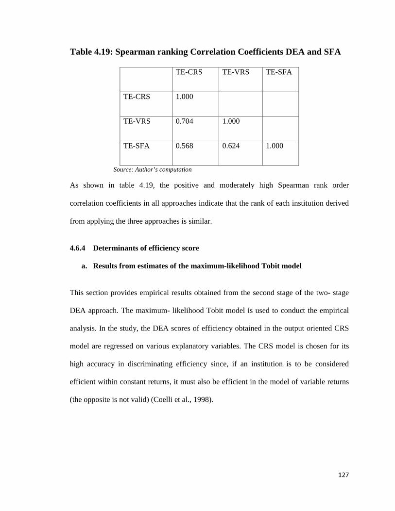
Table 4.19: Spearman ranking Correlation Coefficients DEA and SFA
TE-CRS TE-VRS TE-SFA
TE-CRS 1.000
TE-VRS 0.704 1.000
TE-SFA 0.568 0.624 1.000
Source: Author’s computation
As shown in table 4.19, the positive and moderately high Spearman rank order
correlation coefficients in all approaches indicate that the rank of each institution derived
from applying the three approaches is similar.
4.6.4 Determinants of efficiency score
a. Results from estimates of the maximum-likelihood Tobit model
This section provides empirical results obtained from the second stage of the two- stage
DEA approach. The maximum- likelihood Tobit model is used to conduct the empirical
analysis. In the study, the DEA scores of efficiency obtained in the output oriented CRS
model are regressed on various explanatory variables. The CRS model is chosen for its
high accuracy in discriminating efficiency since, if an institution is to be considered
efficient within constant returns, it must also be efficient in the model of variable returns
(the opposite is not valid) (Coelli et al., 1998).

128
The explanatory variables included in this study are: age (captures experience), size
(captures scale), and other indicators related to ownership, outreach, sustainability and
social performances (see Table 4.20). The institutions’ specific variables or factors
considered in the study are neither inputs nor outputs of the production process, but rather
circumstances faced by decision makers. Determining how these variables influence
efficiency is critical in designing appropriate performance improvement strategies.
Table 4.20: Description of variables along with expected sign
Variables Description Hypothesis
Age Age of MFIs is the number of years since
establishment +
Size Total of all net asset accounts +
Financial self sufficiency Adjusted revenue/Adjusted(Financial Expense
+Impairment Losses on Loans +Operating
Expense)
+
loan size Total value of loans/Number of credit clients -
Ownership 1 if a microfinance institution is government
affiliated4, 0 other wise +
Gender sensitive 1 if a microfinance with more than 50%
women borrowers, 0 other wise -
Debt equity ratio Ratio of total debt to total equity +/-
Capital Asset ratio Ratio of total equity to total assets +/-
4 A microfinance is considered as government affiliated institution if at least 25% its initial capital of ownership

129
The Tobit model used in this study may be specified as :
εα ββββββββ +++++++++=∗
DERCAROwnWomenALSFSSageAssetyi 87654321
(4.10)
Where Asset represents total of all net asset accounts of the i-th microfinance institutions
measured in dollar. In financial institutions asset is usually taken a proxy for size. Larger
size could result in scale efficiency and is expected to have positive effect on efficiency.
However, for institutions which are extremely large, the effect of size could be negative.
Age is age of the i-th microfinance institutions measured in number of years and shows
the experience of the MFI. Matured and experienced institutions are expected to be more
efficient than the young or new institutions. FSS measures microfinance sustainability is
achieved when the operating income of an MFI is sufficient enough to cover all
operational costs. The FSS is expected to have positive impact on efficiency as most
efficient MFIs generate higher returns and thereby are sustainable. Womenitisan
indicator of depth outreach and social orientation of MFIs. It is dummy variable 1 if
MFI has more than 50% women borrowers, 0 otherwise. Higher value for women
indicates more depth of outreach, since lending to women is associated with lending to
poor borrowers (Hermes et al., 2009). Ownership is a dummy variable reflecting 1 if MFI
is government affiliated,0 otherwise.
Table 4.21 provides the descriptive statistics of the explanatory variables included in the
analysis of technical efficiency including their mean, standard deviation, minimum and
maximum values for the sample of 19 MFIs during the period 2004-2009.

130
Table 4.21: Summary of Descriptive Statistics of Variables
Variable Obs Mean Std. Dev. Min Max
Efficiency CRS 114 .672 .242 .115 1
Total asset 114 21041765 43398738 227530 197847309
Age 114 7.342105 2.438006 1 12
Financial sustainability 114 .835 .345249 .28 1.68
Loan size 114 131.0088 56.29434 46 314
Women 114 .4210526 .4959078 0 1
Ownership 114 .3157895 .4668818 0 1
Capital asset ratio 114 .4549123 .2104704 .09 .97
Debt equity ratio 114 1.883421 1.979013 .03 11.15
Source: Author’s computation
Correlation analysis has been conducted to check for potential multicollinearity problem
in the regression. Table 4.22 provides summery on the degree of correlation between the
explanatory variables used. Accordingly, the correlation matrix has shown absence of a
strong relationship among the variables except capital asset ratio and debt equity ratio.

131
Table 4.22: Correlation matrix for independent variables
Asset Age FSS ALS Women Ownership CAR DER
Asset 1
Age 0.487 1
Financial sustainability 0.414 0.331 1
Average Loan size 0.552 0.182 0.181 1
Women -0.119 0.034 -0.113 -0.103 1
Ownership 0.534 0.277 0.248 0.405 -0.312 1
Capital asset ratio -0.341 -0.552 -0.430 -0.170 0.215 -0.256 1
Debt equity ratio 0.256 0.387 0.208 0.093 -0.236 0.370 -0.613 1
Source: Author’s computation

132
In the second stage the CRS DEA technical efficiency scores are regressed on
microfinance specific characteristics in order to identify sources of inefficiencies.
Since efficiency scores range between 0 and 1, Tobit model is employed. Results of the
Tobit estimation are given in Table 4.23. It should be noted that the dependent variable in
the model is DEA efficiency scores. Positive coefficients imply a rise in efficiency,
whereas negative coefficients mean fall in efficiency.
Table 4.23: Results of Tobit Estimation
Coef. Std. Error t-statistic P-value
Constant .428221 .1876429 2.28*** 0.024
Asset 1.84e-09 9.65e-10 1.91* 0.059
Age .0321489 .0110512 2.91*** 0.004
Financial sustainability .07622959 .0433854 1.73* 0.086
Average Loan size .0001521 .0004391 0.35 0.730
Women .0246339 .0444359 0.55 0.580
Ownership .1235756 .0637185 1.94* 0.055
Capital asset ratio -2043459 .1794432 -1.14 0.257
Debt equity ratio -0097538 .017367 -0.56 0.576
Sigma .2076861 .015157
Source: Author’s estimation ***, **, * indicate statistically significant at 1%, 5% and 10% respectively
The result reveals that all the explanatory variables conform to our prior expectation.
However, the result of t - ratio test shows variables asset (size), ownership type, financial
sustainability, and age(experience) are statistically significant. The results indicate that

133
size is positively and significantly related to microfinance’s technical efficiency. This
suggests that large MFIs are more efficient than the small MFIs. This would support the
assumption that large firms tend to enjoy economies of scale. This is consistent with the
findings of Tariq et al (2009). The ownership variable has a significant impact on
efficiency implying that government affiliated MFIs seem to be more efficient than
NGOs and/or Individual owned MFIs. The high efficiency estimates for government
affiliated institutions could be justified by high market share (the four largest MFIs
backed by their respective regional government controls more than 80% of the market).
Institution’s financial sustainability has significant positive effect on efficiency,
indicating that sustainable MFIs are more efficient than the unsustainable MFIs.
Microfinance age is also found to have a positive effect on technical efficiency at 1%
level of significance. This implies that experience leads to a greater capacity for MFIs to
function their activities in a more efficient way. This is consistent with the findings of
Tariq et al. (2009) and Oteng-Abayie et al. (2011). Finally, capita asset ratio¸ debt equity
ratio, average loan size, and targeting women have no significant bearing on technical
efficiency of MFIs.
b. Results from estimates of inefficiency effect model (Using SFA)
For the purpose of consistency and robustness of the results, the empirical finding of the
second stage of DEA is complimented using the one stage SFA proposed by Battese and
Coelli(1992). Following Battese and Celli (1995) model the empirical results are obtained
from an inefficiency effects model using FRONTIER 4.1. That is, the effects of
microfinance- specific variables such as size, ownership type, experience etc up on

134
microfinance’s technical inefficiency are examined in this section. Consequently the
maximum-likelihood estimates for parameters of the stochastic production frontier model
and the technical inefficiency model are estimated simultaneously. The estimated results
are provided in Table 4.24.
Table 4.24: Maximum Likelihood Estimates of the Production Function
Model Parameter Coefficient Standard error t-ratio
Stochastic Frontier Model
Constant β0 0.595* 0.176 3.381
Ln total opert. expenses β1 0.872* 0.130 6.708
Ln number of employees β2 0.383* 0.139 2.755
Technical inefficiency model:
Constant δ0 0.114 0.350 0.326
Time δ1 -0.451* 0.125 -3.608
Total asset δ2 -0.873* 0.209 -4.177
Ownership δ3 -0.132 0.281 -0.469
Age δ4 -0.219* 0.110 -1.991
Financial sustainability δ5 -0.685* 0.121 -5.661
Women δ6 0.669* 0.210 3.185
Sigma-squared σ2 0.252 0.119 2.117
Gamma γ 0.639 0.188 3.399
Log likelihood estimation -39.41
Source: Author’s estimation * shows the significance of variable at 5% level of significance

135
The first part of the Table 4.24 presents the estimated parameters of the production
function while the second part presents the results for inefficiency effects model. The
results of the maximum likelihood estimates of the parameters of the Cobb –Douglas
stochastic production frontier function indicate that the parameters are positive and
significant at 95% confidence interval. The sum of the elasticities of the input variables to
production is higher than unity, i.e., 1.317, signifying increasing returns to scale. Thus
Ethiopian MFIs are operating at the sub-optimal stage (stage I).
The second section of Table 4.24 reports the technical inefficiency model. The result
revealed that all the explanatory variables conform to our prior expectation. However, the
result of t - ratio test shows variables asset, age, financial sustainability, women and trend
are statistically different from zero at 5 percent level of significance. Thus, these
variables are important determinants of efficiency of the MFIs. The negative value of
parameters asset, age, financial sustainability and trend in the technical inefficiency
function indicate the positive influence on the performance of the MFIs. In other words,
asset, age, financial sustainability and time are inversely related with inefficiency
implying that these variables are found to improve efficiency. The negative coefficient of
asset to inefficiency suggests that large MFIs are more efficient than the small MFIs. This
would support the assumption that large firms tend to enjoy economies of scale. The
negative coefficient of age to inefficiency suggests that inefficiency deteriorates as the
microfinance institutions grow. This implies that experience leads to a greater capacity
for MFIs to function their activities in a more efficient way. Coefficient of the variable
financial sustainability is negative indicating that sustainable MFIs are more efficient
than the unsustainable MFIs. The negative coefficient of time implies that technical

136
efficiency increases significantly over time. The positive sign linked to the variable
women is also expected. The positive coefficient of women to inefficiency suggests that
more social oriented MFIs are less efficient. This also shows a tradeoff between
efficiency and outreach which is consistent with the findings of Hermes et al. (2009).
Hypothesis testing for the model
The results of the various hypothesis tests for the model are presented in Table 4.25. All
hypothesis tests are obtained using the generalized likelihood-ratio statistic. The
estimated value of the variance parameter γ = 0.639is statistically significant at the 5%
level, which implies that about 64 percent of the variation in output among the MFIs is
due to the differences inefficiency effect. Null hypothesis, γ =0 which specifies that
inefficiency effects are not stochastic is strongly rejected. Thus, the stochastic frontier
with inefficiency effects is a more appropriate representation than the standard OLS
estimation of the production function. In addition, we test the null hypothesis that the
inefficiency effects are not present, that is, γ = δi = 0 is also rejected at 5% significance
level. For the null hypothesis that all the variables included have no effect on
inefficiency, that is, δi = 0 is rejected. Finally, we test for the null hypothesis that the
technical inefficiency effect has not vary significantly over time. The null hypothesis of
time-invariant inefficiency η = 0 is also rejected at a statistically significant level,
implying that inefficiency varies over time. Thus, the choice of the time-varying decay
model is appropriate.

137
Table 4.25: Generalized likelihood-ratio (LR) tests of null hypotheses (a)
Null hypothesis Test statistics Critical value* Decision
No stochastic ((𝛾 = 0) 43.870 7.045 Reject
No inefficiency(𝛿𝑖 = 0) 21.297 14.853 Reject
No inefficiency effect 40.69 11.911 Reject
Time invariant efficiency (η = 0) 36.605 5.138 Reject
(a)The test statistics have x² distribution with degrees of freedom equal to the difference between the
parameters involved in the null and alternative hypothesis. *All critical values are at 5% level of
significance. The critical values are obtained from table of Kodde and Palm (1986).
The empirical results to determine factors of efficiency obtained from the two-stage DEA
and one stage SFA appear to be consistent. The empirical results of the two-stage DEA
reveal that size, age, ownership and financial sustainability have significant impact on
MFIs technical efficiency. Meanwhile, results of the SFA show that size, age, financial
sustainability, women and time have significant impact on MFIs technical efficiency. The
application of SFA seems to confirm the two-stage DEA as the three factors (size, age
and financial sustainability) appeared to be significant. Therefore, there is strong
evidence from both estimation approaches that institution size, sustainability, and age
(experience) are found to be the main factors that influence efficiency of the Ethiopian
MFIs.

138
4.7 Conclusion
This chapter investigates the technical efficiency of Ethiopian microfinance institutions
using the preferred DEA approach. For the purpose of cross checking and robustness of
the results, the alternative SFA has also been estimated. The results suggest that
Ethiopian MFIs are less efficient with substantial scope to improve their efficiency
performance. The results hold regardless of the different approaches used. The overall
mean efficiency for the MFIs is found to be 67.27%, indicating that MFIs on average
could have increase their output by about 33 % with the existing level of input through
efficient utilization of these inputs. The underperformance in realized microfinance
objectives from the frontier has largely been due technical inefficiency and is largely
within the control of individual microfinance institutions. Further; the results reveal the
prevalence of large variation in the level of technical efficiency across the institutions.
Based on size, large MFIs are found to be the most efficient than the small and medium
sized MFIs. Further, the regression results reveal that asset (size), experience, financial
sustainability and ownership structure have been identified as the most influential
determinants of technical efficiency.
Related Documents