Chapter 9 – Simultaneous Flow of Immiscible Fluids 9.1 An important problem in petroleum engineering is the prediction of oil recovery during displacement by water. Two common examples are a natural water drive and secondary waterflood. The latter is displacement of oil by bottom or edge water, the former is the injection of water to enhance production. In this chapter we will begin with the development of equations of multiphase, immiscible flow, concluding with the frontal advance and Buckley-Leverett equations. Next, we will discuss factors that control displacement efficiency followed by limitations of immiscible displacement solutions. 9.1 Development of equations The development of equations for describing multiphase flow in porous media follows a similar derivation as given previously for single phase, i.e., combination of continuity equation, momentum equation and equation of state. The mass balance of each phase can be written as: increment in time s accumulate that phase of mass increment in time leaving phase of mass increment in time entering phase of mass Shown in Figure 9.1 is the differential element of porous media for oil. u ox │ x u ox │ x+x x y z Figure 9.1 Differential element in Cartesian coordinates. Only x-direction velocity is shown. As an example, the mass of oil entering and leaving the element is given by: Entering: t A u t A u t A u z z oz o y y oy o x x ox o (9.1) Leaving: t A u t A u t A u z z z oz o y y y oy o x x x ox o (9.2) Oil can accumulate by: (1). Change in saturation, (2). Variation of density with temperature and pressure, and (3). Change in porosity due to a change in confining stress. Thus we can write, t o o t t o o V S V S (9.3)

Welcome message from author
This document is posted to help you gain knowledge. Please leave a comment to let me know what you think about it! Share it to your friends and learn new things together.
Transcript

Chapter 9 – Simultaneous Flow of Immiscible Fluids
9.1
An important problem in petroleum engineering is the prediction of oil recovery
during displacement by water. Two common examples are a natural water drive and
secondary waterflood. The latter is displacement of oil by bottom or edge water, the
former is the injection of water to enhance production. In this chapter we will begin with
the development of equations of multiphase, immiscible flow, concluding with the frontal
advance and Buckley-Leverett equations. Next, we will discuss factors that control
displacement efficiency followed by limitations of immiscible displacement solutions.
9.1 Development of equations
The development of equations for describing multiphase flow in porous media
follows a similar derivation as given previously for single phase, i.e., combination of
continuity equation, momentum equation and equation of state. The mass balance of
each phase can be written as:
increment in time saccumulate
thatphase of mass
increment in time
leaving phase of mass
increment in time
entering phase of mass
Shown in Figure 9.1 is the differential element of porous media for oil.
uox│x uox│x+x
x
y z
Figure 9.1 Differential element in Cartesian coordinates. Only x-direction velocity is
shown.
As an example, the mass of oil entering and leaving the element is given by:
Entering: tAutAutAu zzozoyyoyoxxoxo (9.1)
Leaving: tAutAutAu zzzozoyyyoyoxxxoxo
(9.2)
Oil can accumulate by: (1). Change in saturation, (2). Variation of density with
temperature and pressure, and (3). Change in porosity due to a change in confining stress.
Thus we can write,
toottoo VSVS
(9.3)

Chapter 9 – Simultaneous Flow of Immiscible Fluids
9.2
Substitute Eqs. (9.1-9.3) into the conservation of mass expression, rearrange terms, and
take the derivative as t, x, y, z 0, then the phase dependent continuity equations
can be written as;
ooozooyooxo St
uz
uy
ux
(9.4)
wwwzwwywwxw St
uz
uy
ux
(9.5)
The oil and water continuity equations assume no dissolution of oil in the water phase.
That is, no mass transfer occurs between phases and thus flow is immiscible.
The next step is to apply Darcy’s Law to each phase, i. For example in the x-
direction,
x
ku i
i
iixix
(9.6)
where uix is the superficial velocity of phase i in the x-direction, kix, is the effective
permeability to phase i in the x-direction, and is the phase potential. Substitute Eq.
(9.6) into (9.4), apply Leibnitz rule of differentiation, and combine terms, results in,
ooo
o
o
ozoo
o
oyoo
o
oxo St
gz
pk
zy
pk
yx
pk
x
(9.7)
www
w
w
wzww
w
wyww
w
wxw St
gz
pk
zy
pk
yx
pk
x
(9.8)
Even though Eqs. (9.7) and (9.8) are written in Cartesian coordinates, they both can be
solved for a particular geometry. The solution will provide not only pressure and
saturation distributions, but also phase velocities at any point in the porous media.
To combine Eqs. (9.7) and (9.8) requires a relationship between phase pressures
and between phase saturations. The latter is easily understood from the definition of
saturations in Chapter 4, So + Sw = 1.0. The relationship between pressures was
developed in Chapter 5, and is known as capillary pressure.
wP
oPor
wP
nwP
cP (9.9)

Chapter 9 – Simultaneous Flow of Immiscible Fluids
9.3
9.2 Steady state, 1D solution
As a simple example, let’s consider the steady state solution to fluid flow in a
linear system as shown in Figure 9.2. This example is of primary interest in lab
experiments to determine relative permeabilities.
qo
qw L
poi
Pwi
poL
PwL
D
Figure 9.2 Steady state core flood of oil and water.
Oil and water are injected simultaneously, rates and pressures are measured, and core
saturation is determined gravimetrically. Permeability is unknown.
The steady state, incompressible fluid diffusivity equations are given by:
0
0
dx
dpk
dx
d
dx
dpk
dx
d
ww
oo
(9.10)
Integrating and combining with Darcy’s equations,
A
qc
dx
dpk
A
qc
dx
dpk
www
ww
ooo
oo
(9.11)
If water saturation is uniform throughout the core, then effective permeability is
independent of x. Therefore, for oil,
L
oo
o
p
p
o dxk
cdp
oL
oi
(9.12)
which upon integrating, becomes,
)( oLoi
ooo
ppA
Lqk
(9.13)
If kbase = ko at Swi is known, then it is possible to calculate relative permeability.
Chapter 9 – Simultaneous Flow of Immiscible Fluids
9.4
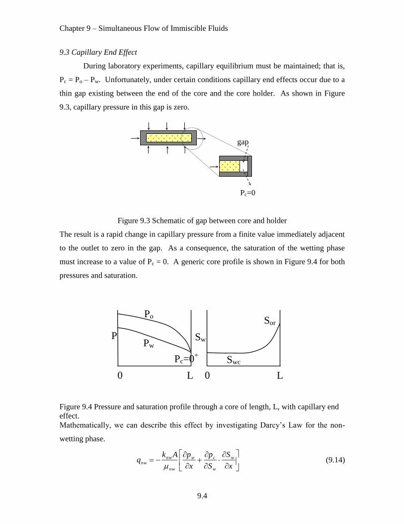
9.3 Capillary End Effect
During laboratory experiments, capillary equilibrium must be maintained; that is,
Pc = Po – Pw. Unfortunately, under certain conditions capillary end effects occur due to a
thin gap existing between the end of the core and the core holder. As shown in Figure
9.3, capillary pressure in this gap is zero.
gap
Pc=0
Figure 9.3 Schematic of gap between core and holder
The result is a rapid change in capillary pressure from a finite value immediately adjacent
to the outlet to zero in the gap. As a consequence, the saturation of the wetting phase
must increase to a value of Pc = 0. A generic core profile is shown in Figure 9.4 for both
pressures and saturation.
Sw
0 0 L L
Po
Pw
Pc=0+ Swc
Sor
P
Figure 9.4 Pressure and saturation profile through a core of length, L, with capillary end
effect.
Mathematically, we can describe this effect by investigating Darcy’s Law for the non-
wetting phase.
x
S
S
p
x
pAkq w
w
cw
nw
nw
nw
(9.14)

Chapter 9 – Simultaneous Flow of Immiscible Fluids
9.5
At the outlet, knw 0, but qnw ≠ 0; therefore,
x
S
Lx
wlim
(9.15)
Two plausible methods have been applied to avoid capillary end effect. The first
is to inject at a sufficiently high rate such that the saturation gradient is driven to a small
region at the end of the core. The second method is to attach a thin, (high porosity and
high permeability) Berea sandstone plug in series with the test core sample. The result is
to confine the saturation gradient in the Berea plug and thus have constant saturation in
the sample of interest.
A consequence of the saturation gradient in the core is that effective permeability
can no longer be considered constant from 0 < x < L. Subsequently, the convenient
steady state method of obtaining relative permeability outlined in Section 9.2 is not valid.
A solution to the saturation gradient can be obtained be combining the definition of
capillary pressure with the steady state, incompressible diffusivity equations. Begin with
defining the boundary conditions. Illustrated in Figure 9.5 is the capillary pressure –
saturation relationship in a core with end effects.
Sw
pc
0
inlet
outlet
Figure 9.5 Schematic representation of capillary pressure – saturation relationship in a
core sample with end effect.
From this figure we can deduce the following conditions,
Pc = 0 for both oil and water phases at x = L.
Sw = Swi at x = 0, thus Pc = Poi – Pwi
Sw = SwL at x = L, thus Pc = 0
From the definition of capillary pressure,

Chapter 9 – Simultaneous Flow of Immiscible Fluids
9.6
dx
dp
dx
dp
dx
dp woc (9.16)
Since pc = f(Sw),
dx
dS
S
p
dx
dp w
w
cc (9.17)
Substituting Eq. (9.17) into (9.16) for the capillary pressure gradient term, and Eq. (9.11)
into (9.16) for the oil and water gradient terms and rearranging, results in,
L
x
S
S
o
oo
w
ww
w
w
c
dx
Ak
q
Ak
q
dSS
pwL
w
(9.18)
Equation (9.18) can be solved either graphically or numerically for saturation gradient.
The result will be a calculated saturation profile similar to the one shown in the right-
hand side of Figure 9.4.
9.4 Frontal advance for unsteady 1D displacement
The unsteady-state displacement of oil by water is due to the change in Sw with
time. This can be visualized by looking at the schematics in Figure 9.6. These
schematics represent
Figure 9.6 Progression of water displacing oil for immiscible, 1D
Swi
Sor
Sw
A
Swi
Sor
Sw
C
0 1x/L
Swi
Sor
Sw
B
Swi
Sor
Sw
D
0 1x/L
Swi
Sor
Sw
A
Swi
Sor
Sw
A
Swi
Sor
Sw
C
0 1x/L
Swi
Sor
Sw
B
Swi
Sor
Sw
B
Swi
Sor
Sw
D
0 1x/L

Chapter 9 – Simultaneous Flow of Immiscible Fluids
9.7
snapshots in time of the frontal boundary as water is displacing oil. In sequence, A
depicts the initial state of the sample (or reservoir) where saturations are separated into
irreducible water, residual oil and mobile oil components. After a given time of
injection, the front advances to a position as shown in B. Ahead of the front water
saturation is at irreducible, but behind the front water saturation is increased. Continuing
in time, eventually the water will breakthrough the end of the core (reservoir) and both oil
and water will be produced simultaneously, C. Continued injection will increase the
displacing phase saturation in the core (reservoir), D.
Two methods to predict the displacement performance are 1) the analytical
solution by Buckley – Leverett (1941), and 2) applying numerical simulation. Only the
analytical solution will be described in this chapter.
9.4.1 Buckley – Leverett (1941)
The derivation begins from the 1D, multiphase continuity equations.
oooxo St
ux
(9.19)
wwwxw St
ux
(9.20)
In terms of volumetric flow rate,
oooo St
Aqx
(9.21)
wwww St
Aqx
(9.22)
Assume the fluids are incompressible and the porosity is constant. Eqs. (9.21) and (9.22)
simplify to,
t
SA
x
q oo
(9.23)
t
SA
x
q ww
(9.24)
Combining,
0
t
SSA
x
qq owow (9.25)
The result is qT = qo + qw = constant, the total flow rate is constant at each cross-section.

Chapter 9 – Simultaneous Flow of Immiscible Fluids
9.8
From the definition of fractional flow,
Two
Tww
qfq
qfq
)1(
(9.26)
Substitute into Darcy’s equation for each phase,
sin)1( gx
pAkqfq o
o
o
oTwo (9.27)
singx
pAkqfq w
w
w
wTww (9.28)
Rearranging Eqs. (9.27) and (9.28), we can substitute into Eq. (9.16) for the pressure
gradient terms. Solving the resulting equation for fractional flow of water, provides the
complete fractional flow equation.
ow
wo
c
To
o
ow
wow
k
k
gx
p
q
Ak
k
kf
1
sin
1
1 (9.29)
In the analytical solution it is difficult to analyze the derivative term (dpc/dx). If we
expand this derivative to,
x
S
S
p
x
p w
w
cc (9.30)
In linear displacement, dpc/dSw 0 at moderate to high water saturations as observed by
the capillary pressure curve such in Figure 9.7. As a result, dpc/dx 0.
Sw
Pc
0
w
c
S
p
Figure 9.7 Capillary pressure curve illustrating flat transition region at moderate to high
water saturations.

Chapter 9 – Simultaneous Flow of Immiscible Fluids
9.9
If the derivative term is negligible, and flow is in the horizontal direction such that no
gravity term is present, then the fractional flow equation reduces to,
ow
wow
k
kf
1
1 (9.31)
If we define mobility ratio as,
wo
ow
k
kM
(9.32)
then fw = 1/(1+1/M).
If we return to Eq. (9.24) and substitute for qw, we obtain,
t
S
q
A
x
f w
T
w
(9.33)
To develop a solution, Eq. (9.33) must be reduced to one dependent variable, either Sw or
fw. Observe, Sw = Sw(x,t) or,
dtt
Sdx
x
SdS
x
w
t
ww
(9.34)
Let dSw(x,t)/dt = 0, (Tracing a fixed saturation plane through the core) then
t
w
x
w
S
xS
tS
dt
dx
w
(9.35)
where the left-hand side is the velocity of the saturation front as it moves through the
porous media.
Observe fw = fw(Sw) only, then,
t
w
tw
w
t
w
x
S
S
f
x
f
(9.36)
Substitution of Eqs. (9.35) and (9.36) into Eq. (9.33), results in the frontal advance
equation.
tw
wT
S S
f
A
q
dt
dx
w
(9.37)

Chapter 9 – Simultaneous Flow of Immiscible Fluids
9.10
Equation (9.37) represents the velocity of the saturation front. Basic assumptions in the
derivation are incompressible fluid, fw(Sw) only and immiscible fluids. Furthermore, only
oil is displaced; i.e., the initial water saturation is immobile, and no initial free gas
saturation exists; i.e., not a depleted reservoir.
The location of the front can be determined by integrating the frontal advance
equation,
dtqS
f
Adx T
t
tw
w
x
S
wS
w
00
1
(9.38)
If injection rate is constant and if the dfw/dSw = f(Sw) only, then
w
w
Sw
wT
S S
f
A
tqx
(9.39)
We can evaluate the derivative from the fractional flow equation (Eq. 9.31), either
graphically or analytical. Figure 9.8 illustrates the graphical solution.
Swf Sw Swc
fw
fwf
Swbt
Figure 9.8 Fractional flow curve
The fractional flow of water at the front, fwf, is determined from the tangent line
originating at Swc. The corresponding water saturation at the front is Swf. The average
water saturation behind the front at breakthrough, Swbt, is given by the intersection at fw =
1. The location of the front is determined by Eq. (9.39), with the slope of the tangent to
the fractional curve used for the derivative function.
Chapter 9 – Simultaneous Flow of Immiscible Fluids
9.11
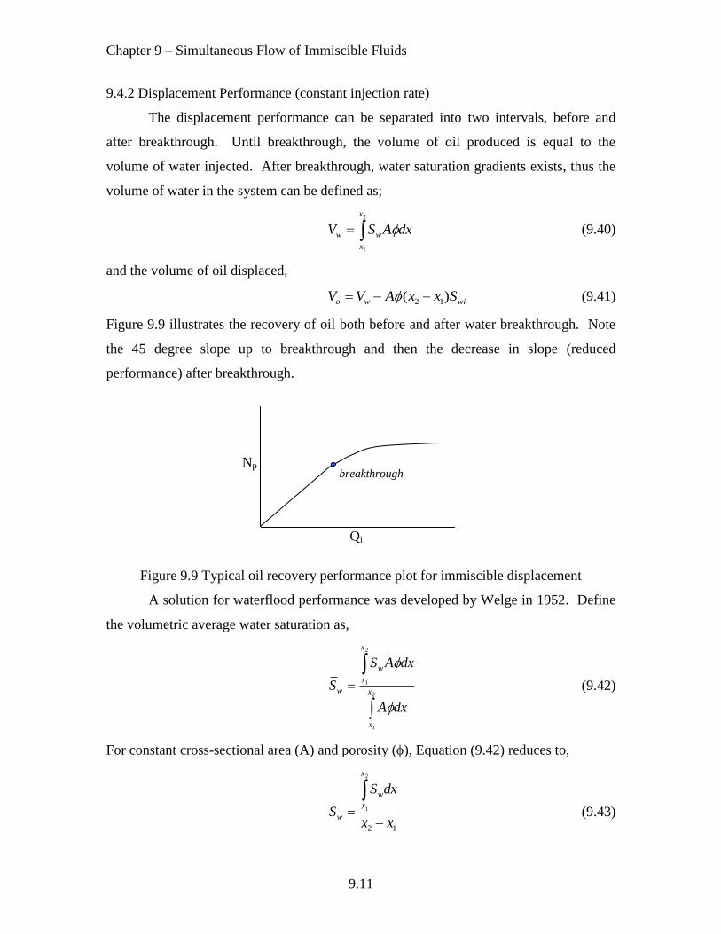
9.4.2 Displacement Performance (constant injection rate)
The displacement performance can be separated into two intervals, before and
after breakthrough. Until breakthrough, the volume of oil produced is equal to the
volume of water injected. After breakthrough, water saturation gradients exists, thus the
volume of water in the system can be defined as;
2
1
x
x
ww dxASV (9.40)
and the volume of oil displaced,
wiwo SxxAVV )( 12 (9.41)
Figure 9.9 illustrates the recovery of oil both before and after water breakthrough. Note
the 45 degree slope up to breakthrough and then the decrease in slope (reduced
performance) after breakthrough.
Np
Qi
breakthrough
Figure 9.9 Typical oil recovery performance plot for immiscible displacement
A solution for waterflood performance was developed by Welge in 1952. Define
the volumetric average water saturation as,
2
1
2
1
x
x
x
x
w
w
dxA
dxAS
S
(9.42)
For constant cross-sectional area (A) and porosity (), Equation (9.42) reduces to,
12
2
1
xx
dxS
S
x
x
w
w
(9.43)

Chapter 9 – Simultaneous Flow of Immiscible Fluids
9.12
The integrand can be expanded and the equation rearranged such that,
2
11212
1122 1w
www dSx
xxxx
SxSxS (9.44)
Substitute the frontal advance equation (Eq. 9.37) for the integral and solve,
12
2
1
2
1
wwT
w
Sw
wT
ffA
tq
dSS
f
A
tqdSwx
w
(9.45)
Thus the general Welge equation is,
12
12
12
1122
xx
ff
A
tq
xx
SxSxS wwTww
w
(9.46)
A useful simplification is to consider x1 = 0 at the inlet and x2 = L at the outlet end of the
core,
22 1 wT
ww fLA
tqSS
(9.47)
where fw1 is assumed to be one at the inlet.
Define the total volume injected, Wi, = qT*t, and the pore volume, Vp = AL. Combining
gives the number of pore volumes injected, Qi,
p
ii
V
WQ (9.48)
Thus we can write Eq. (9.47) in terms of Qi.
22 1 wiww fQSS (9.49)
The cumulative oil displaced, Np, can be expressed in terms of the difference in the
average water saturation and the exit end saturation, i.e.,
2wwpp SSVN (9.50)
Consider a special case immediately before breakthrough. In this case, Sw2 = Swi and fw2
= 0. Subsequently, Eq. (9.49) can be written as:
ibtwiwbt QSS (9.51)
and the cumulative oil displaced:
wiwbtpp SSVN (9.52)

Chapter 9 – Simultaneous Flow of Immiscible Fluids
9.13
9.4.3 Determination of relative permeability curves
Continuing from the previous section, the objective is to determine relative
permeability curves from linear displacement data. Writing Equation (9.49) in terms of
fractional flow of oil, fo,
022 fQSS iww (9.53)
Next, calculate ko/kw from the fractional flow equation.
1
1
22
ww
o
Sw
o
fk
k
w
(9.54)
In this example, both gravity and capillary pressure components are considered negligible
and thus are ignored. The average fractional flow of oil at the exit end for a given time
increment is given by,
i
WpWWp
ii
p
oW
NN
WdW
dNf iii
0
lim2 (9.55)
where dNp is cumulative oil produced and dWi is water injected during t. Alternative
expressions for dNp and dWi can be written as,
ii
wp
dQLAdW
SdLAdN
(9.56)
which results in a useful expression for fo2.
i
ww
i
wo
Q
SS
dQ
Sdf 2
2
(9.57)
The slope of a plot of average water saturation vs PVs of water injected provides an
estimate of fo2 (Figure 9.10).
Sw
Qi
breakthrough
0
Sw2
Figure 9.10 Plot of average water saturation vs Qi for determining fo2.

Chapter 9 – Simultaneous Flow of Immiscible Fluids
9.14
To estimate the permeability of each phase, begin with the Darcy multiphase flow
equation written in terms of pressure drop.
L
w
rw
o
rob
T
kkAk
dxqp
0
(9.58)
Pressure drop is measured across the core during the constant rate test. From the single
phase, steady state experiment we obtain,
b
bbb
p
LqAk
(9.59)
Define effective apparent viscosity,-1
, as:
1
1
w
rw
o
ro kk
(9.60)
Substitute Eqs. (9.59) and (9.60) into Eq. (9.58),
L
bb
bT dx
Lq
pqp
0
(9.61)
Define the average apparent viscosity as:
x
x
dx
dx
0
0
1
1
(9.62)
thus at the outlet end, x = L, Eq. (9.61) becomes,
bT
bb
pq
pq
1 (9.63)
Calculation of individual relative permeabilities requires values of -1
at known
saturations. For example, at the outlet end, where Sw2 is known,
1
2
2
1
2
2
wwrw
ooro
fk
fk
(9.64)
where the exit end apparent viscosity can be determined from the following relationship.

Chapter 9 – Simultaneous Flow of Immiscible Fluids
9.15
i
idQ
dQ
111
2
(9.65)
The derivative can be evaluated from the slope of a plot of the inverse of average
apparent viscosity vs. PVs water injected as shown in figure 9.11.
-1
Qi
breakthrough
Figure 9.11 Plot of inverse of average apparent viscosity vs Qi for determining fo2.
Example 9.1
An unsteady state test was performed at constant injection rate for the purpose of
determining the oil and water relative permeability curves. Table 1 lists the input
parameters for the test.
Swi = 0.35
Vp = 31.13 cc
w = 0.97 cp
o = 10.45 cp
q = 80 cc/hr
pb/qb= 0.1245 psi/cc/hr
Table 1 – Input Parameters

Chapter 9 – Simultaneous Flow of Immiscible Fluids
9.16
cumulative Cumulative
wtr injection oil produced p Qi Swave fo2 Sw2 fw2 kro/krw
Wi, (cc) Np, (cc) psi (PV)
0.00 0.00 138.6 0.000 0.350 1.000 0.350 0.000
3.11 3.11 120.4 0.100 0.450 1.000 0.350 0.000
7.00 7.00 97.5 0.225 0.575 0.585 0.443 0.415 15.166
11.20 7.84 91.9 0.360 0.602 0.154 0.546 0.846 1.963
16.28 8.43 87.9 0.523 0.621 0.083 0.577 0.917 0.980
24.27 8.93 83.7 0.780 0.637 0.038 0.607 0.962 0.425
39.20 9.30 78.5 1.259 0.649 0.019 0.625 0.981 0.208
62.30 9.65 74.2 2.001 0.660 0.009 0.641 0.991 0.103
108.90 9.96 70.0 3.498 0.670 0.005 0.653 0.995 0.053
155.60 10.11 68.1 4.998 0.675 0.002 0.666 0.998 0.018
311.30 10.30 65.4 10.000 0.681 0.001 0.669 0.999 0.013
Table 2. Calculations for relative permeability ratio
0.30
0.35
0.40
0.45
0.50
0.55
0.60
0.65
0.70
0.0 0.5 1.0 1.5 2.0
Qi
Sw
ave
Figure 1. Plot of average water saturation vs. pore volume water injected. Slope provides
exit end fractional flow of oil.
p fo2 fw2 Qi average m*
psi (PV) -1
2-1
Sw2 krw kro
138.6 1.000 0.000 0.000 13.50 13.50 0.350 0.000 0.774
120.4 1.000 0.000 0.100 11.73 -17.80 13.50 0.350 0.000 0.774
97.5 0.585 0.415 0.225 9.50 -10.68 11.90 0.443 0.034 0.514
91.9 0.154 0.846 0.360 8.95 -3.14 10.08 0.546 0.081 0.160
87.9 0.083 0.917 0.523 8.56 -1.90 9.56 0.577 0.093 0.091
83.7 0.038 0.962 0.780 8.15 -1.24 9.12 0.607 0.102 0.043
78.5 0.019 0.981 1.259 7.65 -0.76 8.60 0.625 0.111 0.023
74.2 0.009 0.991 2.001 7.23 -0.37 7.97 0.641 0.121 0.012
70.0 0.005 0.995 3.498 6.82 -0.20 7.51 0.653 0.129 0.007
68.1 0.002 0.998 4.998 6.63 -0.07 6.98 0.666 0.139 0.003
65.4 0.001 0.999 10.000 6.37 -0.05 6.90 0.669 0.141 0.002
Table 3. Calculations to determine relative permeabilites
Chapter 9 – Simultaneous Flow of Immiscible Fluids
9.17
0
2
4
6
8
10
12
14
16
0.0 5.0 10.0 15.0
Qi
-1
)av
e
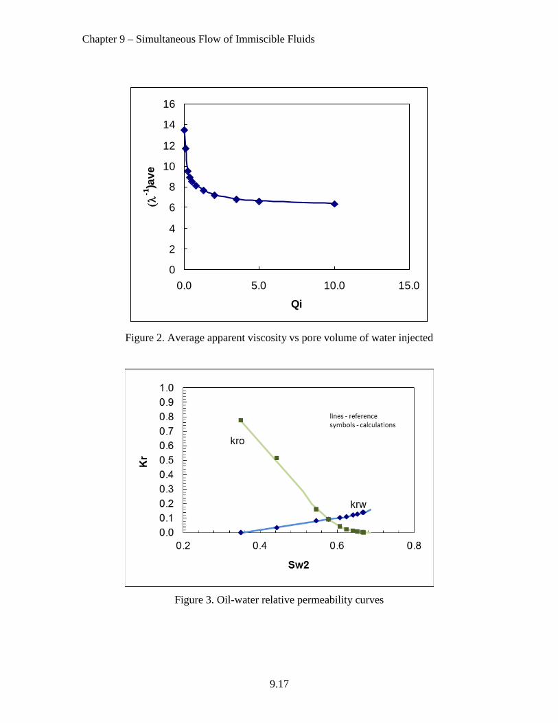
Figure 2. Average apparent viscosity vs pore volume of water injected
Figure 3. Oil-water relative permeability curves

Chapter 9 – Simultaneous Flow of Immiscible Fluids
9.18
Step-by-step procedure
Measured data includes cumulative water injection (Wi), cumulative oil produced (Np)
and pressure drop (p) as shown in Table 2.
Step 1:
Calculate the cumulative pore volumes of water injected, Qi from Eq. 9.48.
p
ii
V
WQ
Step 2:
Calculate the average water saturation from Eq. 9.50.
p
p
wiwV
NSS
Step 3:
Calculate the exit end fractional flow of oil from the slope of Figure 1.
i
wo
Q
Sf
2
Step 4:
Calculate the exit end water saturation from Eq. 9.49.
22 oiww fQSS
Step 5:
Calculate exit end fractional flow of water by,
022 1 ffw
Step 6:
Calculate the relative permeability ratio as shown in Table 2 from Eq. 9.54.
1
1
22
ww
o
Sw
o
fk
k
w
Step 7:
Find the average apparent viscosity from Eq. 9.63.
bT
bb
pq
pq
1

Chapter 9 – Simultaneous Flow of Immiscible Fluids
9.19
Step 8:
Find the slope of the average apparent viscosity vs Qi plot, Figure 2.
iQm
1
*
Step 9:
Calculate the exitend apparent viscosity from Eq. 9.65. Results shown in Table 3.
*11
2 mQi
Step 10:
Calculate the individual relative permeabilities with respect to the outlet end,
where Sw2 is known,
1
2
2
1
2
2
wwrw
ooro
fk
fk
Results are shown in Table 3 and Figure 3, respectively.
9.4.4 Displacement Performance (constant pressure)
In some cases it is more advantageous to perform an experiment at a constant pressure
differential. As a result the injection rate is allowed to vary with time. One such
example, is the linear displacement of oil by gas. This technique of determining oil and
gas relative permeabilities by the unsteady state method is known as “gasflooding”.
The following data were obtained in a laboratory experiment to determine the relative gas
and oil permeability. Plot kro, krg vs. So.
Pinlet = 2.0 atm, abs
Poutlet = 1.0 atm, abs
o = 1.2 cp
g = 0.018 cp
Vp =180 cm3
qo = 0.40 cc/sec

Chapter 9 – Simultaneous Flow of Immiscible Fluids
9.20
Time (secs) Cumulative
gas injection
(cc)
Cumulative
oil produced
(cc)
0 0 0
104 50 42.5
134 75 49.0
199 150 56.0
238 200 58.5
276 250 60.3
381 400 63.7
447 500 65.5
518 600 66.3
577 700 67.4
635 800 68.1
693 900 69.0
750 1000 69.7
Solution
A laboratory experiment was run with a constant pressure drop between the inlet and
outlet. Measured were time, cumulative gas injected, and cumulative oil produced. Also
known are the oil and gas viscosities, pore volume of the sample and the single phase oil
rate prior to gas injection…saturate the core with oil, steady state process, at irreducible
water saturation.
Step 1: Plot cumulative oil production (Np) vs time. Determine oil flow rate by,
dt
pdN
oq
Step 2: Calculate the cumulative gas injected in terms of mean pressure and expressed in
pore volumes.
)
oP
iP(
iP2
pV
iG
)pv(i
Q
Step 3: Calculate the average gas saturation by,
giS
pV
pN
gS
Step 4: Determine the oil cut from the slope of a plot of average gas saturation vs Qi

Chapter 9 – Simultaneous Flow of Immiscible Fluids
9.21
idQ
gSd
of
Step 5: Determine the relative permeability ratio,
o
g
of
of1
rok
rgk
Step 6: Calculate the saturation at the outflow face
o
fi
Qg
Sg
S *2
Step 7: Determine kro by Darcy’s Law,
4.0
)t(o
q
oiq
)t(o
q
pA
Looi
q
pA
Lo
)t(o
q
k
ok
rok
Step 8: Determine the gas relative permeability
ro
k*
nrok
rgk
rgk
time
secs
Cumulative
Gas injection,
Gi, (cc)
Cumulative
oil produced
Np, (cc)
production
rate
qo (cc/sec)
Cumulative
Gas injection,
Qi, (pv)
Average gas
saturation Sg
oil cut
fo
0 0 0 0 0 0 1
104 50 42.5 0.366 0.370 0.236 0.490
134 75 49.0 0.142 0.556 0.272 0.101
199 150 56.0 0.091 1.111 0.311 0.057
238 200 58.5 0.056 1.481 0.325 0.032
276 250 60.3 0.036 1.852 0.335 0.020
381 400 63.7 0.030 2.963 0.354 0.016
447 500 65.5 0.019 3.704 0.364 0.010
518 600 66.3 0.015 4.444 0.368 0.007
577 700 67.4 0.015 5.185 0.374 0.007
635 800 68.1 0.014 5.926 0.378 0.006
693 900 69.0 0.014 6.667 0.383 0.006
750 1000 69.7 0.012 7.407 0.387 0.005
Chapter 9 – Simultaneous Flow of Immiscible Fluids
9.22
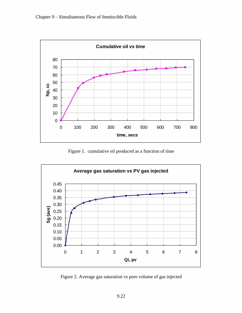
Figure 1. cumulative oil produced as a function of time
Figure 2. Average gas saturation vs pore volume of gas injected
Cumulative oil vs time
0
10
20
30
40
50
60
70
80
0 100 200 300 400 500 600 700 800
time, secs
Np
, cc
Average gas saturation vs PV gas injected
0.00
0.05
0.10
0.15
0.20
0.25
0.30
0.35
0.40
0.45
0 1 2 3 4 5 6 7 8
Qi, pv
Sg
(av
e)

Chapter 9 – Simultaneous Flow of Immiscible Fluids
9.23
Figure 3. Oil and gas relative permeability curves as a function of exit end oil saturation
Cumulative
Gas injection,
Qi, (pv)
Average gas
saturation Sg krg/kro ratio
Exit end
saturation
Sg2
Exit end
saturation
So2 Kro Krg
0 0 0 0 1 1.000 0
0.37 0.236 0.016 0.055 0.945 0.914 0.014
0.56 0.272 0.133 0.216 0.784 0.355 0.047
1.11 0.311 0.248 0.248 0.752 0.228 0.057
1.48 0.325 0.450 0.277 0.723 0.140 0.063
1.85 0.335 0.754 0.299 0.701 0.091 0.069
2.96 0.354 0.947 0.308 0.692 0.076 0.072
3.70 0.364 1.523 0.328 0.672 0.047 0.072
4.44 0.368 2.090 0.337 0.663 0.037 0.076
5.19 0.374 2.207 0.339 0.661 0.038 0.085
5.93 0.378 2.485 0.343 0.657 0.034 0.086
6.67 0.383 2.485 0.343 0.657 0.035 0.086
7.41 0.387 2.842 0.348 0.652 0.031 0.087
Gas/oil relative permeability curves
0.0
0.1
0.2
0.3
0.4
0.5
0.6
0.7
0.8
0.9
1.0
0 0.1 0.2 0.3 0.4 0.5 0.6 0.7 0.8 0.9 1
So2
Kro
or
krg
krg
kro

Chapter 9 – Simultaneous Flow of Immiscible Fluids
9.24
9.5 Factors that control displacement efficiency
Before discussing the effect of various factors on displacement efficiency, we will
begin with an elaboration on “mobility ratio”. It is the most widely-used lumped
parameter used to estimate displacement performance. The general definition given by
Eq. (9.31) does not fully describe the terms. Consider a sharp front as illustrated in
Figure 9.11.
Sor
Swi
w)Sor
w)Swf o)Swi
Figure 9.11 Schematic of a sharp front in immiscible displacement including location of
mobility terms.
In this case, the mobility ratio is defined as the mobility of the displacing phase behind
the front to the mobility of the displaced phase ahead of the front.
d
DM
(9.66)
where,
wi
or
So
ood
Sw
wwD
k
k
(9.67)
Note both permeabilities are evaluated at the endpoints, Swi and Sor, respectively.
If no sharp front is evident, we define the “apparent mobility ratio”, Ms, as:
wiwf Sro
o
Sw
rws
k
kM
(9.68)
where the water mobility is evaluated at the average water saturation behind the front.
The apparent mobility ratio is a measure of the relative rate of oil movement ahead of the

Chapter 9 – Simultaneous Flow of Immiscible Fluids
9.25
front to the water movement behind the front, assuming the oil and water pressure
gradients are equal. Therefore, if
Ms < 1 oil rate > water rate….high displacement
Ms = 1 oil rate = water rate
Ms > 1 oil rate < water rate….poor displacement efficiency
The result is displacement efficiency (ED) decreases as apparent mobility increases as
shown schematically in Figure 9.12.
ED
Qi(pv)
Ms
3 1
5
Figure 9.12 Effect of apparent mobility ratio on displacement efficiency
In general form,
d
i
Sd
Si
M
(9.69)
where i is the mobility of the injected fluid evaluated at the average saturation of the
injected fluid at breakthrough, and d is the mobility of the displaced fluid evaluated at
the average saturation of the displaced fluid. Typical values are Ms of 0.2 to 10 for water
displacing oil, up to Ms of 1000 for gas displacing oil.
Wettability
The shape of the relative permeability curves are influenced by wettability, subsequently
impacting mobility ratio and fractional flow. Figure 9.13 illustrates the effect of
wettability on the fractional flow of water.

Chapter 9 – Simultaneous Flow of Immiscible Fluids
9.26
Sw
=47°
Slightly Water wet
fw
oil wet
=180°
Figure 9.13 Effect of wettability on fractional flow of water
A decrease in water wetness, results in an increase in krw and a corresponding decrease in
kro. The mobility term increases and thus becomes more unfavorable; i.e., poorer
displacement efficiency. Figure 9.14 illustrates the decrease in efficiency in terms of
pore volumes of oil produced vs pore volumes of water injected.
Np
(pv)
Qi(pv)
47°
2.5
0.4
0
0.3
180°
Incremental due
to wettability
Figure 9.14 Effect of apparent mobility ratio on displacement efficiency
Interfacial Tension
Recovery efficiency for displacement of oil by water is a weak function of the
interfacial tension. As shown in Figure 9.15, the difference in oil recovery is minimal for
a large range of interfacial tensions.

Chapter 9 – Simultaneous Flow of Immiscible Fluids
9.27
Np
(pv)
Qi(pv)
=0.5
0.4
0
=40
Figure 9.15 Effect of interfacial tension on displacement efficiency
Recall, capillary pressure is a function of interfacial tension. In displacement, the
capillary pressure gradient is included in the fractional flow (See Eq. 9.29). Therefore,
the weak function suggests capillary pressure is not a dominant component of
displacement.
Viscosity Ratio
As the viscosity of oil increases the mobility ratio will correspondingly increase,
resulting in an increase in the fractional flow of water. Figure 9.16 illustrates the effect
for three arbitrary viscosity ratios, 100, 10 and 1, respectively.
Sw
o/w= fw
100 10 1
Figure 9.16 Effect of viscosity ratio on fractional flow of water
In fact, according to Eq. 9.31, as M increases, then fw 1.0. The oil recovery for various
viscosity ratios can be seen in Figure 9.17.

Chapter 9 – Simultaneous Flow of Immiscible Fluids
9.28
Np
(pv)
Qi(pv)
o=1.8cp
0
Incremental due
to oil viscosity
o=151cp
Figure 9.17 Effect of viscosity ratio on displacement efficiency
The ultimate recovery is independent of the viscosity ratio; however, the time to recover
the oil is highly dependent on the ratio.
Gravity
The influence of gravity on displacement can be explained by observing the
reservoir configuration shown in Figure 9.18.
wtr
oil
Figure 9.18. Stratigraphic reservoir configuration
By definition, = o – w in the fractional flow equation for water (Eq. 9.29).
Assuming gravity is (+) upwards, then since o < w gravity will reduce the fractional
flow of water when the water is moving updip. Conversely, water injected at the crest of
the structure will move faster under the influence of gravity. The subsequent
displacement efficiency and oil recovery are less in this case.
9.6 Residual oil saturation
After displacement, there exists a remaining oil saturation known as the residual
oil saturation. It is dependent on wettability, pore size distribution, microscopic
heterogeneity and properties of the displacing fluids. As an example, consider for water

Chapter 9 – Simultaneous Flow of Immiscible Fluids
9.29
wet rock the oil is trapped as globules or ganglia. But for oil wet rock the oil is trapped
as a film on the grain surfaces. The importance of understanding the residual oil
saturation is it establishes a maximum efficiency for oil displaced by water on the
microscopic level. Furthermore, it is the initial oil saturation for the next possible phase
of development; i.e., EOR.
The measure of the effectiveness of the displacement process is defined by the
microscopic displacement efficiency, ED.
11 /
/1
by water contactedd/unit waterflooof beginningat OIP stock tank
by water contacted Vprecovered/ oil stock tank
oo
oo
D
BS
BS
E
(9.70)
Where, So1 is the volumetric average oil saturation at the beginning of the waterflood and
So is the volumetric average oil saturation at a particular point during the waterflood. The
oil displaced is given by;
1
1
o
opwDp
B
SVEN
w (9.71)
where Npw is the oil displaced by water and Vpw is the pore volume swept by water to the
volumetric average residual oil saturation.
The dependence of residual oil saturation on capillary and viscous forces was
verified by a series of experiments. Using dimensional analysis, define Capillary
Number, NCA, as the ratio of viscous to capillary forces.
cosow
wCA
vN (9.72)
Where v is the interstitial velocity (u/) and w is the viscosity of the displacing fluid.
Experimental data was obtained by measuring the oil saturation in cores when the first
water is detected at the outlet. Since the oil volume produced after breakthrough is small,
the results represent the trapping process. Figure 9.19 illustrates the general behavior of
the reduction in oil saturation in the core at breakthrough with increasing capillary
number.

Chapter 9 – Simultaneous Flow of Immiscible Fluids
9.30
0 NCA 10
-8 10
-3
50
So,%
pv
Figure 9.19 Reduction of oil saturation at breakthrough vs capillary number
At smaller capillary numbers, capillary forces dominate. With increasing capillary
number the viscous forces become more dominate.
A modification of the original definition of capillary number was developed for
waterfloods at constant injection rate.
4.0
cos)(
o
w
oworoi
wCAM
SS
vN
(9.73)
The following guidelines are suggested.
NCAM < 10-6
capillary forces dominate
10-4
< NCAM < 10-5
transition
NCAM > 10-4
viscous forces dominate
Correlating residual oil saturation with capillary and viscous forces has several
important implications for fluid flow in porous media. It demonstrates the independence
of Sor from flood velocity at reservoir rates. Furthermore, correlations illustrate that Sor
can be reduced below field waterflood residual in the laboratory corefloods if the lab
experiments are conducted at large NCAM.
In many field applications reservoir pressure has depleted to the point where
appreciable free gas saturation exists in the pores. Subsequently, prior to water injection
both a residual oil and gas saturation co-exist. If re-pressurization occurs during water
injection, the gas will dissolve back into the oil with little, if any, effect on the residual oil
saturation. However, if a trapped gas saturation is present at the time the residual oil is
trapped by water, a substantial reduction of residual oil saturation will occur. For
example, a correlation shown in Figure 9.20 illustrates the reduction in residual oil
saturation for a water-wet, consolidated rock. Implied in the figure is that an increase in

Chapter 9 – Simultaneous Flow of Immiscible Fluids
9.31
initial flowing gas saturation is proportional to an increase in trapped gas saturation and
thus a reduction in residual oil saturation.
Sgi,%
10
0 30
S
or,%
Figure 9.20 Reduction in Sor for increasing initial gas saturation
9.7 Limitations of the frontal advance solution
In development of the frontal advance solution several limitations are evident.
Based on the assumptions in deriving the solution, the fluids were considered immiscible
and incompressible. Furthermore, the porous media was assumed isotropic and
homogeneous, with uniform saturation distributions. And last, only one-dimensional,
linear flow was illustrated.
The frontal advance solution applies to a stabilized displacement process. In
other words, the displacement behavior is independent of injection rate and length of the
sample. Two parameters which must meet the criteria are the breakthrough saturation
and the recovery vs PV injected after breakthrough. An empirical correlation from
dimensional analysis was developed to determine if a flood was at stabilized conditions.
}/{75.762.0
}{1085.510835.0
2
99
daycpftto
NxtoxLu wT
(9.74)
The left-hand-side is known as the “critical scaling coefficient”. If the numerical value of
this coefficient exceeds the critical value, then stabilized flow will occur. Since rate and
length effects occur when capillary forces become important in the displacement process,
this scaling factor also indicates when capillary forces are minimized. In applications,
under field conditions the displacement process is almost always stable. Under lab
conditions, to compute relative permeabilities from linear displacement tests, it is
Chapter 9 – Simultaneous Flow of Immiscible Fluids
9.32
necessary to estimate the operating conditions to obtain stabilized flow. Two examples
from Willhite (1986) illustrate the point.
Example 1
A reservoir is 1000 ft long, and was flooded at an average frontal velocity of 1 ft/day.
The porosity of the reservoir is 19% and the displacing fluid viscosity is 0.7 cp. Estimate
the scaling coefficient and determine whether the displacement was stabilized.
Solution
In oilfield units, the value of uT = 0.19 ft/day (=1 ft/day*.19). Thus,
daycpftLu wT /133)7.0)(19.0)(1000( 2
This value is an order of magnitude greater than the critical values observed in lab
experiments, and therefore flow is stabilized.
Example 2
It is desired to conduct a laboratory waterflood experiment under stabilized conditions in
a core 2.54 cm in diameter and 5 cm long. The porosity of the core is 15% and the
viscosity is 1 cp [1 kPa-s]. Estimate the volumetric injection rate in cubic meters/second
if the critical scaling coefficient is 5.85 x 10⁻⁹
N.
Solution
TTwT uxsPaumLu 5105)001.0)()(05.0(
Substituting the critical value, results in uT = 1.17x10⁻⁴
m/s. Subsequently, the
volumetric rate becomes,
smxq
mxAuq T
/1093.5
)0254.0(4
1017.1
38
24
Related Documents