Chapter 9 Correlation and Regression 1. Chapter Outline 9.1 Correlation 9.2 Linear Regression 9.3 Measures of Regression and Prediction Intervals 9.4.

Chapter 9

Correlation and Regression

1

Chapter Outline

• 9.1 Correlation

• 9.2 Linear Regression

• 9.3 Measures of Regression and Prediction Intervals

• 9.4 Multiple Regression

2

Section 9.1

Correlation

3

Section 9.1 Objectives

• Introduce linear correlation, independent and dependent variables, and the types of correlation

• Find a correlation coefficient

• Test a population correlation coefficient ρ using a table

• Perform a hypothesis test for a population correlation coefficient ρ

• Distinguish between correlation and causation

4

Correlation

Correlation

• A relationship between two variables.

• The data can be represented by ordered pairs (x, y) x is the independent (or explanatory) variable y is the dependent (or response) variable

5

Correlation

x 1 2 3 4 5

y – 4 – 2 – 1 0 2

A scatter plot can be used to determine whether a linear (straight line) correlation exists between two variables.

x

2 4

–2

– 4

y

2

6

Example:

6

Types of Correlation

x

y

Negative Linear Correlation

x

y

No Correlation

x

y

Positive Linear Correlation

x

y

Nonlinear Correlation

As x increases, y tends to decrease.

As x increases, y tends to increase.

7

Example: Constructing a Scatter Plot

A marketing manager conducted a study to determine whether there is a linear relationship between money spent on advertising and company sales. The data are shown in the table. Display the data in a scatter plot and determine whether there appears to be a positive or negative linear correlation or no linear correlation.

Advertisingexpenses,($1000), x

Companysales

($1000), y2.4 2251.6 1842.0 2202.6 2401.4 1801.6 1842.0 1862.2 215

8

Solution: Constructing a Scatter Plot

x

y

Advertising expenses(in thousands of

dollars)

Com

pany

sal

es(i

n th

ousa

nds

of

dolla

rs)

Appears to be a positive linear correlation. As the advertising expenses increase, the sales tend to increase.

9

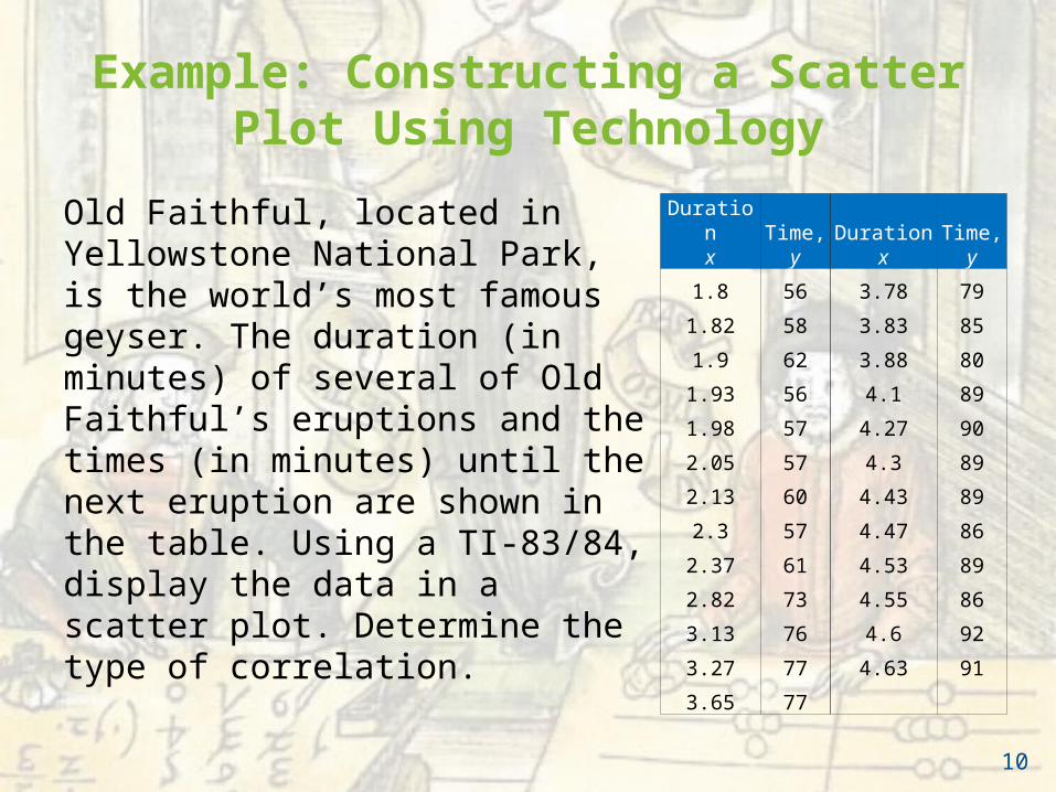
Example: Constructing a Scatter Plot Using Technology

Old Faithful, located in Yellowstone National Park, is the world’s most famous geyser. The duration (in minutes) of several of Old Faithful’s eruptions and the times (in minutes) until the next eruption are shown in the table. Using a TI-83/84, display the data in a scatter plot. Determine the type of correlation.

Durationx

Time,y

Durationx

Time,y

1.8 56 3.78 79

1.82 58 3.83 85

1.9 62 3.88 80

1.93 56 4.1 89

1.98 57 4.27 90

2.05 57 4.3 89

2.13 60 4.43 89

2.3 57 4.47 86

2.37 61 4.53 89

2.82 73 4.55 86

3.13 76 4.6 92

3.27 77 4.63 91

3.65 77    

10

Solution: Constructing a Scatter Plot Using Technology

• Enter the x-values into list L1 and the y-values into list L2.

• Use Stat Plot to construct the scatter plot.STAT > Edit… STATPLOT

From the scatter plot, it appears that the variables have a positive linear correlation.

11

1 550

100

Correlation Coefficient

Correlation coefficient

• A measure of the strength and the direction of a linear relationship between two variables.

• The symbol r represents the sample correlation coefficient.

• A formula for r is

• The population correlation coefficient is represented by ρ (rho). 2 22 2

n xy x yr

n x x n y y

n is the number of data pairs

12

Slide 9- 13

How to calculate r, the sample correlation coefficient, using Ti-84.

Correlation Coefficient

• The range of the correlation coefficient is -1 to 1.

-1 0 1

If r = -1 there is a perfect negative

correlation

If r = 1 there is a perfect positive

correlation

If r is close to 0 there is no linear

correlation

14

Linear Correlation

Strong negative correlation

Weak positive correlation

Strong positive correlation

Nonlinear Correlation

x

y

x

y

x

y

x

y

r = 0.91 r = 0.88

r = 0.42 r = 0.07

15

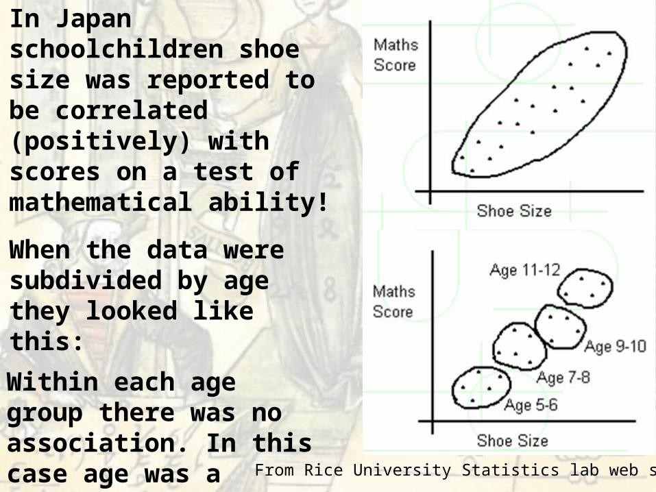
In Japan schoolchildren shoe size was reported to be correlated (positively) with scores on a test of mathematical ability!

When the data were subdivided by age they looked like this:

Within each age group there was no association. In this case age was a confounding variable. From Rice University Statistics lab web site

Much of the interest in red wine comes from the observation that the French (who have a long tradition of drinking red wine) often have healthy hearts and arteries despite typically having high-fat foods in their diet. But studies show that people who drink wine over other types of alcohol tend to live healthier lives, smoking less, drinking less and having a healthier diet. So these other factors, rather than the red wine, may in fact be responsible for their good health.

Slide 9- 18© 2012 Pearson Education, Inc.

The benefit of drinking red wine was discovered as a result of a two-year-long experiment involving 220 people with type 2 diabetes. They kept to a standard Mediterranean diet, not restricted by calories, but were randomized into three groups – those who drank 150 ml of mineral water after dinner, and either white wine or red wine. The group of red wine drinkers got higher levels of the so-called “good cholesterol,” or HDL, which helps fight “bad cholesterol,” or LDL, and also protects against heart attacks and strokes. In general, people with diabetes are more predisposed to heart diseases than the general population.

Finishing each dinner with a glass of red wine might be a good idea for people with diabetes, Israeli researchers claim.

http://rt.com/news/256525-red-wine-diabetes-heart

Slide 9- 19© 2012 Pearson Education, Inc.

Solution: All the benefits of red wine without the devastating effects of alcohol! Alcohol is removed using low heat and centrifuge!

Still, many doctors agree that something in red wine appears to help your heart. It's possible that antioxidants, such as flavonoids or a substance called resveratrol, have heart-healthy benefits.

Slide 9- 20© 2012 Pearson Education, Inc.

This is the executive summary of the statement of the American Statistical Association on the use of value-added assessment to evaluate teachers. Please share it with other teachers, with principals, and school board members. Please share it with your legislators and other elected officials. Send it to your local news outlets. The words are clear: Teachers account for between 1 and 14% of the variation in test scores. And this is very important to remember: “Ranking teachers by their VAM scores can have unintended consequences that reduce quality.”

How much does a teacher account for students’ success (or failure) at school?

http://dianeravitch.net/2014/11/22/every-teacher-in-the-u-s-should-post-this-statement-in-his-or-her-classroom/

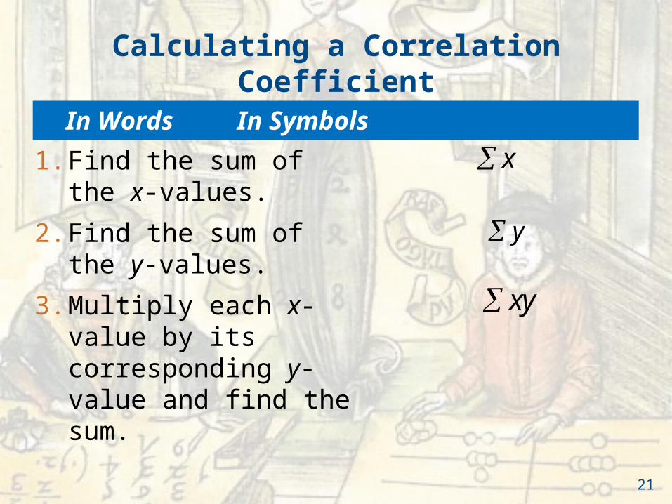
Calculating a Correlation Coefficient

1. Find the sum of the x-values.

2. Find the sum of the y-values.

3. Multiply each x-value by its corresponding y-value and find the sum.

x

y

xy

In Words In Symbols

21

Calculating a Correlation Coefficient

4. Square each x-value and find the sum.

5. Square each y-value and find the sum.

6. Use these five sums to calculate the correlation coefficient.

2x

2y

2 22 2

n xy x yr

n x x n y y

In Words In Symbols

22

Example: Finding the Correlation Coefficient

Calculate the correlation coefficient for the advertising expenditures and company sales data. What can you conclude?

Advertisingexpenses,($1000), x

Companysales

($1000), y2.4 2251.6 1842.0 2202.6 2401.4 1801.6 1842.0 1862.2 215

23

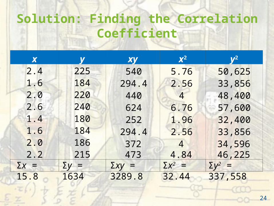
Solution: Finding the Correlation Coefficient

x y xy x2 y2

2.4 2251.6 1842.0 2202.6 2401.4 1801.6 1842.0 1862.2 215

540294.4440624252

294.4372473

5.762.56

46.761.962.56

44.84

50,62533,85648,40057,60032,40033,85634,59646,225

Σx = 15.8 Σy = 1634 Σxy = 3289.8 Σx2 = 32.44 Σy2 = 337,558

24

Solution: Finding the Correlation Coefficient

2 22 2

n xy x yr

n x x n y y

2 2

8(3289.8) 15.8 1634

8(32.44) 15.8 8(337,558) 1634

501.2 0.91299.88 30,508

Σx = 15.8 Σy = 1634 Σxy = 3289.8 Σx2 = 32.44 Σy2 = 337,558

r ≈ 0.913 suggests a strong positive linear correlation. As the amount spent on advertising increases, the company sales also increase.

25

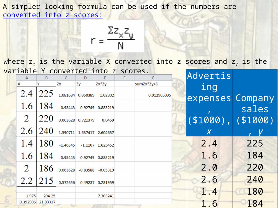
A simpler looking formula can be used if the numbers are converted into z scores:

where zx is the variable X converted into z scores and zy is the variable Y converted into z scores.

Advertisingexpenses,($1000), x

Companysales

($1000), y2.4 2251.6 1842.0 2202.6 2401.4 1801.6 1842.0 1862.2 215

Example: Using Technology to Find a Correlation Coefficient

Use a technology tool to calculate the correlation coefficient for the Old Faithful data. What can you conclude?

Durationx

Time,y

Durationx

Time,y

1.8 56 3.78 79

1.82 58 3.83 85

1.9 62 3.88 80

1.93 56 4.1 89

1.98 57 4.27 90

2.05 57 4.3 89

2.13 60 4.43 89

2.3 57 4.47 86

2.37 61 4.53 89

2.82 73 4.55 86

3.13 76 4.6 92

3.27 77 4.63 91

3.65 77    

27

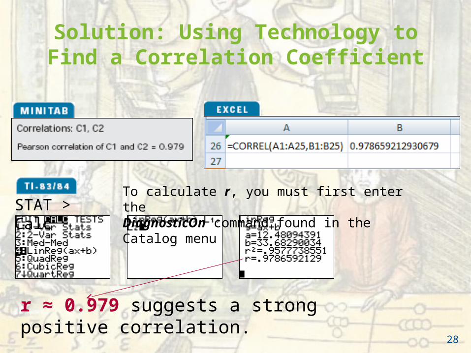
Solution: Using Technology to Find a Correlation Coefficient

STAT > CalcTo calculate r, you must first enter the DiagnosticOn command found in the Catalog menu

r ≈ 0.979 suggests a strong positive correlation.

28

Slide 9- 29

How to calculate r, the sample correlation coefficient, using Ti-84.

Using a Table to Test a Population Correlation Coefficient ρ

• Once the sample correlation coefficient r has been calculated, we need to determine whether there is enough evidence to decide that the population correlation coefficient ρ is significant at a specified level of significance.

• Use Table 11 in Appendix B.

• If |r| is greater than the critical value, there is enough evidence to decide that the correlation coefficient ρ is significant.

30

Using a Table to Test a Population Correlation Coefficient ρ

• Determine whether ρ is significant for five pairs of data (n = 5) at a level of significance of α = 0.01.

• If |r| > 0.959, the correlation is significant. Otherwise, there is not enough evidence to conclude that the correlation is significant.

Number of pairs of data in sample

level of significance

31

Using a Table to Test a Population Correlation Coefficient ρ

1. Determine the number of pairs of data in the sample.

2. Specify the level of significance.

3. Find the critical value.

Determine n.

Identify .

Use Table 11 in Appendix B.

In Words In Symbols

32

Using a Table to Test a Population Correlation Coefficient ρ

In Words In Symbols

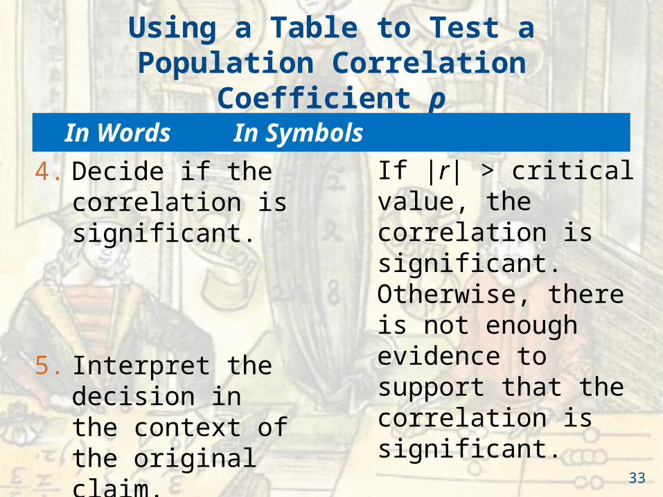
4. Decide if the correlation is significant.

5. Interpret the decision in the context of the original claim.

If |r| > critical value, the correlation is significant. Otherwise, there is not enough evidence to support that the correlation is significant.

33

Example: Using a Table to Test a Population Correlation Coefficient ρ

Using the Old Faithful data, you used 25 pairs of data to find r ≈ 0.979. Is the correlation coefficient significant? Use α = 0.05.

Durationx

Time,y

Durationx

Time,y

1.8 56 3.78 79

1.82 58 3.83 85

1.9 62 3.88 80

1.93 56 4.1 89

1.98 57 4.27 90

2.05 57 4.3 89

2.13 60 4.43 89

2.3 57 4.47 86

2.37 61 4.53 89

2.82 73 4.55 86

3.13 76 4.6 92

3.27 77 4.63 91

3.65 77    

34

Solution: Using a Table to Test a Population Correlation Coefficient ρ

• n = 25, α = 0.05

• |r| ≈ 0.979 > 0.396

• There is enough evidence at the 5% level of significance to conclude that there is a significant linear correlation between the duration of Old Faithful’s eruptions and the time between eruptions.

35

Hypothesis Testing for a Population Correlation Coefficient ρ

• A hypothesis test can also be used to determine whether the sample correlation coefficient r provides enough evidence to conclude that the population correlation coefficient ρ is significant at a specified level of significance.

• A hypothesis test can be one-tailed or two-tailed.

36

Hypothesis Testing for a Population Correlation Coefficient ρ

• Left-tailed test

• Right-tailed test

• Two-tailed test

H0: ρ 0 (no significant negative correlation)

Ha: ρ < 0 (significant negative correlation)

H0: ρ 0 (no significant positive correlation)

Ha: ρ > 0 (significant positive correlation)

H0: ρ = 0 (no significant correlation)

Ha: ρ 0 (significant correlation)

37

The t-Test for the Correlation Coefficient

• Can be used to test whether the correlation between two variables is significant.

• The test statistic is r

• The standardized test statistic:

follows a t-distribution with d.f. = n – 2.

• In this text, only two-tailed hypothesis tests for ρ are considered.

212

0

r

r rtr

n

38

Using the t-Test for ρ

1. State the null and alternative hypothesis.

2. Specify the level of significance.

3. Identify the degrees of freedom.

4. Determine the critical value(s) and rejection region(s).

State H0 and Ha.

Identify .

d.f. = n – 2.

Use Table 5 in Appendix B.

In Words In Symbols

39

Using the t-Test for ρ

5. Find the standardized test statistic.

6. Make a decision to reject or fail to reject the null hypothesis.

7. Interpret the decision in the context of the original claim.

In Words In Symbols

If t is in the rejection region, reject H0. Otherwise fail to reject H0.

212

rtr

n

40

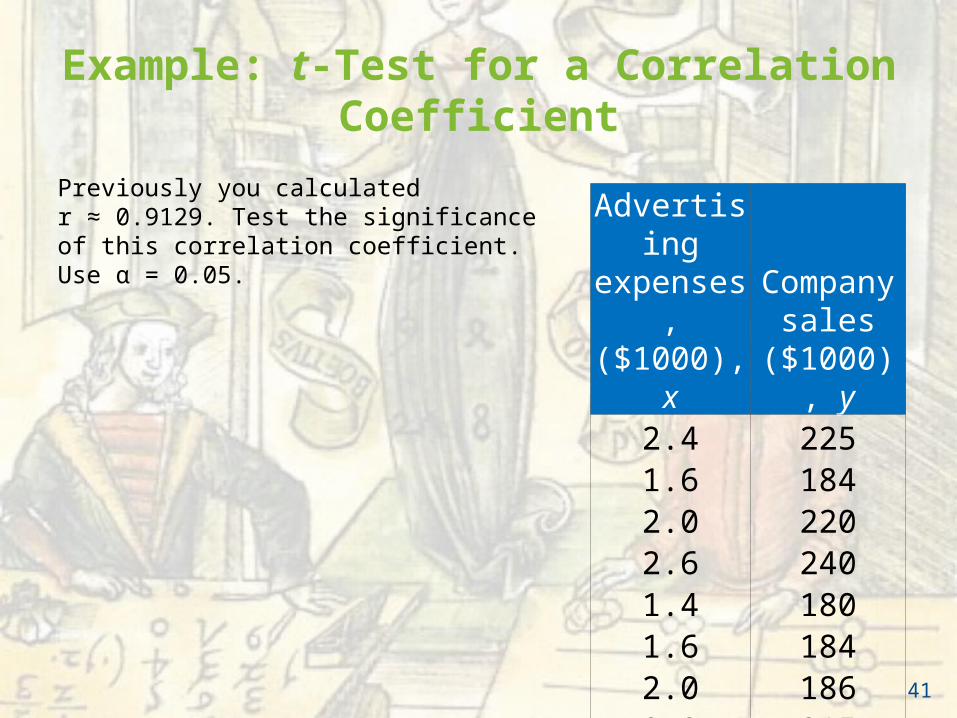
Example: t-Test for a Correlation Coefficient

Previously you calculated r ≈ 0.9129. Test the significance of this correlation coefficient. Use α = 0.05.

Advertisingexpenses,($1000), x

Companysales

($1000), y2.4 2251.6 1842.0 2202.6 2401.4 1801.6 1842.0 1862.2 215

41

t0-2.447

0.025

2.447

0.025

Solution: t-Test for a Correlation Coefficient

• H0:

• Ha:

•

• d.f. =

• Rejection Region:

• Test Statistic:

0.058 – 2 = 6

2

0.9129 05.478

1 (0.9129)8 2

t

ρ = 0ρ ≠ 0

-2.447 2.447

5.478

• Decision:At the 5% level of significance, there is enough evidence to conclude that there is a significant linear correlation between advertising expenses and company sales.

Reject H0

42

s is the standard error about the line, a measure of the typical size of a residual (the numbers stored in ∟RESID). It is the square root of the sum of squares of the residuals divided by the degrees of freedom. Smaller values indicate that the points tend to be close to the fitted line, while large values indicate scattering.

Correlation and Causation

• The fact that two variables are strongly correlated does not in itself imply a cause-and-effect relationship between the variables.

• If there is a significant correlation between two variables, you should consider the following possibilities.1. Is there a direct cause-and-effect relationship

between the variables?• Does x cause y?

44

Correlation and Causation

2. Is there a reverse cause-and-effect relationship between the variables?• Does y cause x?

3. Is it possible that the relationship between the variables can be caused by a third variable or by a combination of several other variables?

4. Is it possible that the relationship between two variables may be a coincidence?

45

Section 9.1 Summary

• Introduced linear correlation, independent and dependent variables and the types of correlation

• Found a correlation coefficient

• Tested a population correlation coefficient ρ using a table

• Performed a hypothesis test for a population correlation coefficient ρ

• Distinguished between correlation and causation

46

Section 9.2

Linear Regression

47

Section 9.2 Objectives

• Find the equation of a regression line

• Predict y-values using a regression equation

48

Regression lines

• After verifying that the linear correlation between two variables is significant, next we determine the equation of the line that best models the data (regression line).

• Can be used to predict the value of y for a given value of x.

x

y

49

Residuals

Residual

• The difference between the observed y-value and the predicted y-value for a given x-value on the line.

For a given x-value,

di = (observed y-value) – (predicted y-value)

x

y

}d1

}d2

d3{d4{ }d5

d6{

Predicted y-value

Observed y-value

50

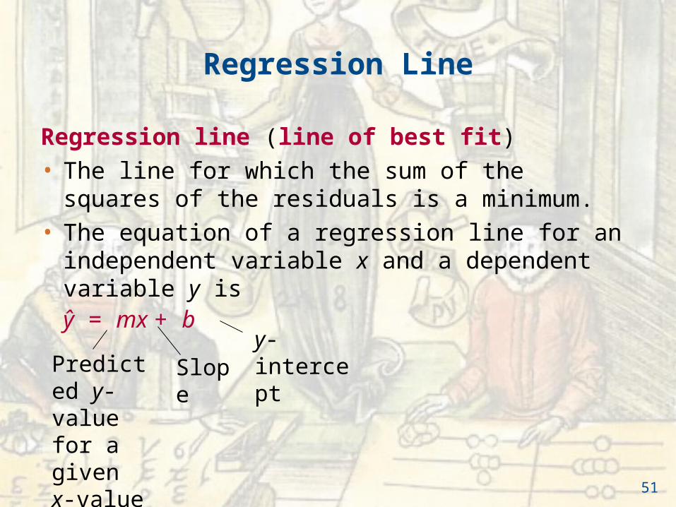
Regression line (line of best fit)

• The line for which the sum of the squares of the residuals is a minimum.

• The equation of a regression line for an independent variable x and a dependent variable y is

ŷ = mx + b

Regression Line

Predicted y-value for a given x-value

Slopey-intercept

51

22

y

x

sn xy x ym r

sn x x

y xb y mx mn n

52

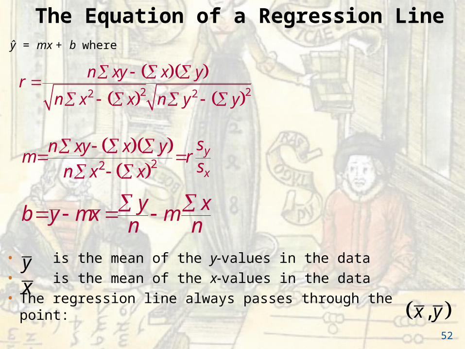
2 22 2

n xy x yr

n x x n y y

The Equation of a Regression Lineŷ = mx + b where

• is the mean of the y-values in the data

• is the mean of the x-values in the data

• The regression line always passes through the point:

yx

,x y

Example: Finding the Equation of a Regression Line

Find the equation of the regression line for the advertising expenditures and company sales data.

Advertisingexpenses,($1000), x

Companysales

($1000), y2.4 2251.6 1842.0 2202.6 2401.4 1801.6 1842.0 1862.2 215

53

Solution: Finding the Equation of a Regression Line

x y xy x2 y2

2.4 2251.6 1842.0 2202.6 2401.4 1801.6 1842.0 1862.2 215

540294.4440624252

294.4372473

5.762.56

46.761.962.56

44.84

50,62533,85648,40057,60032,40033,85634,59646,225

Σx = 15.8 Σy = 1634 Σxy = 3289.8 Σx2 = 32.44 Σy2 = 337,558

Recall from section 9.1:

54

Solution: Finding the Equation of a Regression Line

Σx = 15.8 Σy = 1634 Σxy = 3289.8 Σx2 = 32.44 Σy2 = 337,558

22

n xy x ym

n x x

b y mx

28(3289.8) (15.8)(1634)

8(32.44) 15.8

501.2 50.728749.88

1634 15.8(50.72874)8 8

204.25 (50.72874)(1.975) 104.0607

ˆ 50.729 104.061y x Equation of the regression line

55

Solution: Finding the Equation of a Regression Line

• To sketch the regression line, use any two x-values within the range of the data and calculate the corresponding y-values from the regression line.

ˆ 50.729 104.061y x

x

Advertising expenses(in thousands of dollars)

Com

pany

sal

es(i

n th

ousa

nds

of d

olla

rs) y

56

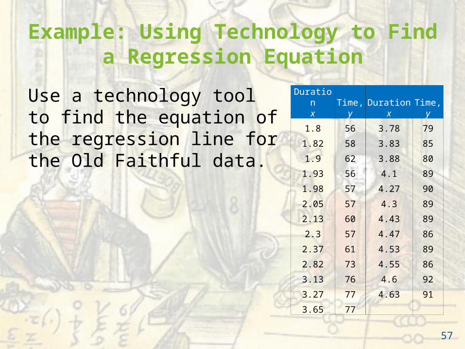
Example: Using Technology to Find a Regression Equation

Use a technology tool to find the equation of the regression line for the Old Faithful data.

Durationx

Time,y

Durationx

Time,y

1.8 56 3.78 79

1.82 58 3.83 85

1.9 62 3.88 80

1.93 56 4.1 89

1.98 57 4.27 90

2.05 57 4.3 89

2.13 60 4.43 89

2.3 57 4.47 86

2.37 61 4.53 89

2.82 73 4.55 86

3.13 76 4.6 92

3.27 77 4.63 91

3.65 77    

57

58

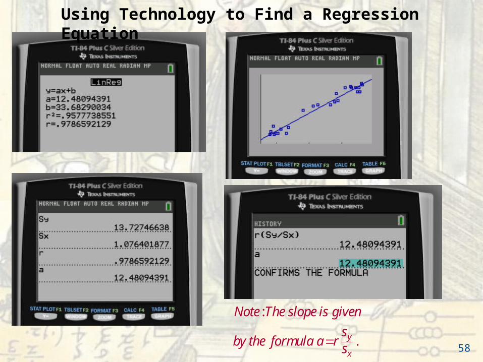
Using Technology to Find a Regression Equation

:

.y

x

Note The slope is given

sby the formula a r

s

Example: Predicting y-Values Using Regression Equations

The regression equation for the advertising expenses (in thousands of dollars) and company sales (in thousands of dollars) data is ŷ = 50.729x + 104.061. Use this equation to predict the expected company sales for the following advertising expenses. (Recall from section 9.1 that x and y have a significant linear correlation.)

1.1.5 thousand dollars

2.1.8 thousand dollars

3.2.5 thousand dollars

59

60

ŷ =50.729(1.5) + 104.061 ≈ 180.155

ŷ =50.729(1.8) + 104.061 ≈ 195.373

ŷ =50.729(2.5) + 104.061 ≈ 230.884

Solution: Predicting y-Values Using Regression Equations

ŷ = 50.729x + 104.061

1. 1.5 thousand dollars

When the advertising expenses are $1500, the company sales are about $180,155.

ŷ =50.729(1.5) + 104.061 ≈ 180.155

• 1.8 thousand dollars

When the advertising expenses are $1800, the company sales are about $195,373.

ŷ =50.729(1.8) + 104.061 ≈ 195.373

61

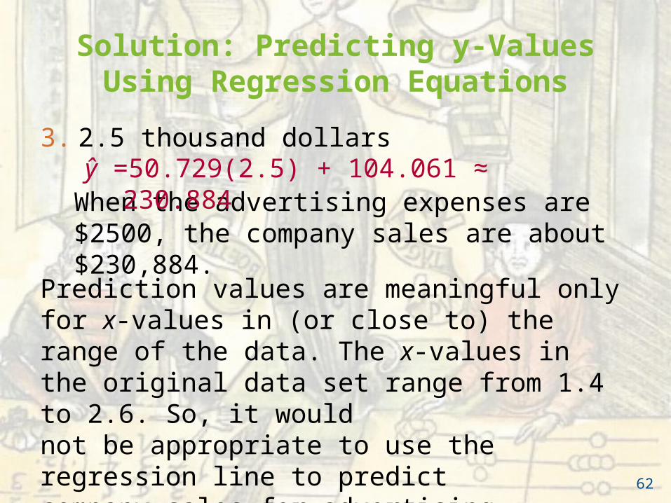
Solution: Predicting y-Values Using Regression Equations

3. 2.5 thousand dollars

When the advertising expenses are $2500, the company sales are about $230,884.

ŷ =50.729(2.5) + 104.061 ≈ 230.884

Prediction values are meaningful only for x-values in (or close to) the range of the data. The x-values in the original data set range from 1.4 to 2.6. So, it wouldnot be appropriate to use the regression line to predictcompany sales for advertising expenditures such as 0.5 ($500) or 5.0 ($5000).

62

Section 9.2 Summary

• Found the equation of a regression line

• Predicted y-values using a regression equation

63

Section 9.3

Measures of Regression and Prediction Intervals

64

Section 9.3 Objectives

• Interpret the three types of variation about a regression line

• Find and interpret the coefficient of determination

• Find and interpret the standard error of the estimate for a regression line

• Construct and interpret a prediction interval for y

65

Variation About a Regression Line

• Three types of variation about a regression line Total variation Explained variation Unexplained variation

• To find the total variation, you must first calculate The total deviation The explained deviation The unexplained deviation

66

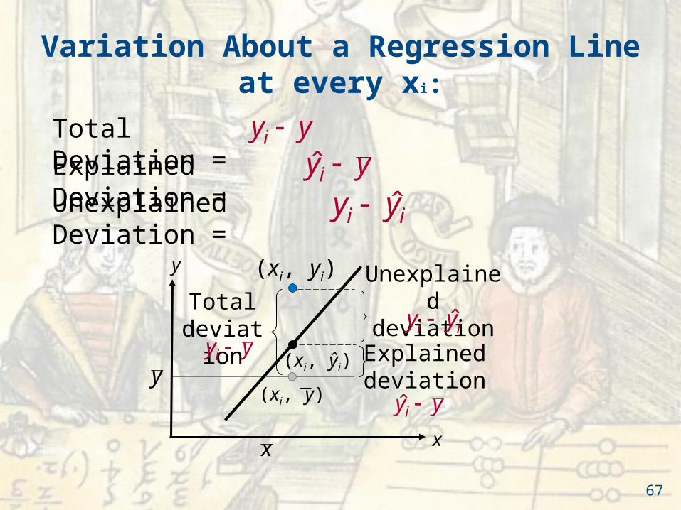
Variation About a Regression Line at every xi:

iy yˆiy y

ˆi iy y

(xi, ŷi)

x

y (xi, yi)

(xi, y)

Unexplained deviation

ˆi iy yTotal

deviationiy y Explained

deviationˆiy y

y

x

Total Deviation =

Explained Deviation =

Unexplained Deviation =

67

Total variation

• The sum of the squares of the differences between the y-value of each ordered pair and the mean of y.

Explained variation

• The sum of the squares of the differences between each predicted y-value and the mean of y.

Variation About a Regression Line

2iy y Total variation =

Explained variation = 2ˆiy y

68

Unexplained variation

• The sum of the squares of the differences between the y-value of each ordered pair and each corresponding predicted y-value.

Variation About a Regression Line

2ˆi iy y Unexplained variation =

The sum of the explained and unexplained variation is equal to the total variation.

69

Total variation = Explained variation + Unexplained variation

= + 2iy y 2

ˆiy y 2ˆi iy y

Coefficient of determination

• The ratio of the explained variation to the total variation.

• Denoted by r2

22

2ˆExplained variation

Total variationi

i

y yr

y y

70

Coefficient of Determination

Use a technology tool to find the equation of the regression line for the Old Faithful data. We can confirm the formula:

Durationx

Time,y

Durationx

Time,y

1.8 56 3.78 79

1.82 58 3.83 85

1.9 62 3.88 80

1.93 56 4.1 89

1.98 57 4.27 90

2.05 57 4.3 89

2.13 60 4.43 89

2.3 57 4.47 86

2.37 61 4.53 89

2.82 73 4.55 86

3.13 76 4.6 92

3.27 77 4.63 91

3.65 77     71

22

2ˆExplained variation

Total variationi

i

y yr

y y

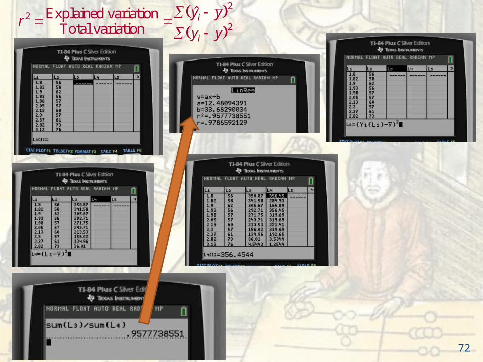
72

22

2ˆExplained variation

Total variationi

i

y yr

y y

Example: Coefficient of Determination

22 (0.913)

0.834

r

About 83.4% of the variation in the company sales can be explained by the variation in the advertising expenditures. About 16.6% of the variation is unexplained.

The correlation coefficient for the advertising expenses and company sales data as calculated in Section 9.1 isr ≈ 0.913. Find the coefficient of determination. What does this tell you about the explained variation of the data about the regression line? About the unexplained variation?Solution:

73

The Standard Error of Estimate

Standard error of estimate

• The standard deviation of the observed yi -values about the predicted ŷ-value for a given xi -value.

• Denoted by se.

• The closer the observed y-values are to the predicted y-values, the smaller the standard error of estimate will be.

2( )ˆ2

i ie

y ys

n

n is the number of ordered pairs in the data set

74

The Standard Error of Estimate

2

, , , ( ), ˆ ˆ( )ˆ

i i i i i

i i

x y y y yy y

1. Make a table that includes the column heading shown.

2. Use the regression equation to calculate the predicted y-values.

3. Calculate the sum of the squares of the differences between each observed y-value and the corresponding predicted y-value.

4. Find the standard error of estimate.

ˆ iy mx b

2 ( )ˆi iy y

2( )ˆ2

i ie

y ys

n

In Words In Symbols

75

Example: Standard Error of Estimate

The regression equation for the advertising expenses and company sales data as calculated in section 9.2 is

ŷ = 50.729x + 104.061

Find the standard error of estimate.

Solution:Use a table to calculate the sum of the squared differences of each observed y-value and the corresponding predicted y-value.

76

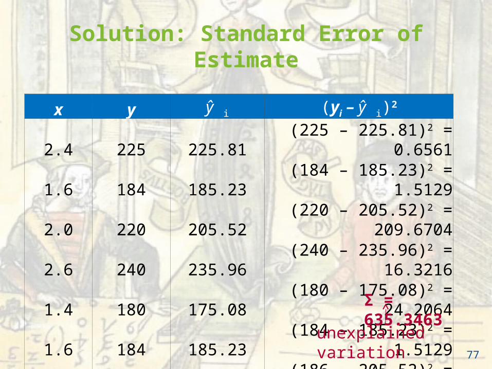
Solution: Standard Error of Estimate

x y ŷ i (yi – ŷ i)2

2.4 225 225.81 (225 – 225.81)2 = 0.65611.6 184 185.23 (184 – 185.23)2 = 1.51292.0 220 205.52 (220 – 205.52)2 = 209.67042.6 240 235.96 (240 – 235.96)2 = 16.32161.4 180 175.08 (180 – 175.08)2 = 24.20641.6 184 185.23 (184 – 185.23)2 = 1.51292.0 186 205.52 (186 – 205.52)2 = 381.03042.2 215 215.66 (215 – 215.66)2 = 0.4356

Σ = 635.3463

unexplained variation77

Solution: Standard Error of Estimate

• n = 8, Σ(yi – ŷ i)2 = 635.3463

2( )ˆ2

i ie

y ys

n

The standard error of estimate of the company sales for a specific advertising expense is about $10.29.

635.3463 10.2908 2

78

Prediction Intervals

• Two variables have a bivariate normal distribution if for any fixed value of x, the corresponding values of y are normally distributed and for any fixed values of y, the corresponding x-values are normally distributed.

79

Prediction Intervals

• A prediction interval can be constructed for the true value of y.

• Given a linear regression equation ŷ = mx + b and x0, a specific value of x, a c-prediction interval for y is

ŷ – E < y < ŷ + E where

• The point estimate is ŷ and the margin of error is E. The probability that the prediction interval contains y is c.

202 2

( )11( )c e

n x xE t s

n n x x

80

Constructing a Prediction Interval for y for a Specific Value of x

1. Identify the number of ordered pairs in the data set n and the degrees of freedom.

2. Use the regression equation and the given x-value to find the point estimate ŷ.

3. Find the critical value tc that corresponds to the given level of confidence c.

ˆi iy mx b

Use Table 5 in Appendix B.

In Words In Symbols

d.f. = n – 2

81

Constructing a Prediction Interval for y for a Specific Value of x

4. Find the standard error of estimate se.

5. Find the margin of error E.

6. Find the left and right endpoints and form the prediction interval.

In Words In Symbols2( )ˆ

2i i

ey y

sn

2

02 2

( )11( )c e

n x xE t s

n n x x

Left endpoint: ŷ – E Right endpoint: ŷ + E Interval: ŷ – E < y < ŷ + E

82

Example: Constructing a Prediction Interval

Construct a 95% prediction interval for the company sales when the advertising expenses are $2100. What can you conclude?

Recall, n = 8, ŷ = 50.729x + 104.061, se = 10.290

Solution:Point estimate: ŷ = 50.729(2.1) + 104.061 ≈ 210.592

Critical value:d.f. = n –2 = 8 – 2 = 6 tc = 2.447

215.8, 32.44, 1.975x x x

83

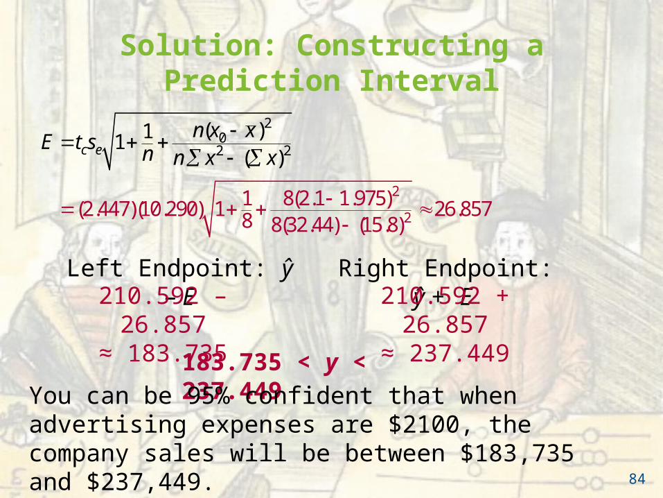
Solution: Constructing a Prediction Interval

0

2

2

2

2 2

1 8(2.1 1.975)(2.447)(10.290) 1 26.8578 8(32.44) (15

( )

8)

1

.

1( )c e

n x xE t s

n n x x

Left Endpoint: ŷ – E Right Endpoint: ŷ + E

183.735 < y < 237.449

210.592 – 26.857≈ 183.735

210.592 + 26.857≈ 237.449

You can be 95% confident that when advertising expenses are $2100, the company sales will be between $183,735 and $237,449.

84

Slide 9- 85© 2012 Pearson Education, Inc.

0

2

2

2

2 2

1 8(2.1 1.975)(2.447)(10.290) 1 26.8578 8(32.44) (15

( )

8)

1

.

1( )c e

n x xE t s

n n x x

All the values necessary to calculate Eare found under the VARS/ Statistics (5).s value is found after doing a LinRegTTest.

Section 9.3 Summary

• Interpreted the three types of variation about a regression line

• Found and interpreted the coefficient of determination

• Found and interpreted the standard error of the estimate for a regression line

• Constructed and interpreted a prediction interval for y

86

Section 9.4

Multiple Regression

87

Section 9.4 Objectives

• Use technology to find a multiple regression equation, the standard error of estimate and the coefficient of determination

• Use a multiple regression equation to predict y-values

88

Multiple Regression Equation

• In many instances, a better prediction can be found for a dependent (response) variable by using more than one independent (explanatory) variable.

• For example, a more accurate prediction for the company sales discussed in previous sections might be made by considering the number of employees on the sales staff as well as the advertising expenses.

89

Multiple Regression Equation

Multiple regression equation • ŷ = b + m1x1 + m2x2 + m3x3 + … + mkxk

• x1, x2, x3,…, xk are independent variables

• b is the y-intercept

• y is the dependent variable

* Because the mathematics associated with this concept is complicated, technology is generally used to calculate the multiple regression equation.

90

Example: Finding a Multiple Regression Equation

A researcher wants to determine how employee salaries at a certain company are related to the length of employment, previous experience, and education. The researcher selects eight employees from the company and obtains the data shown on the next slide. Use Minitab to find a multiple regression equation that models the data.

91

Example: Finding a Multiple Regression Equation

Employee Salary, yEmployment

(yrs), x1

Experience (yrs), x2

Education (yrs), x3

A 57,310 10 2 16B 57,380 5 6 16C 54,135 3 1 12D 56,985 6 5 14E 58,715 8 8 16F 60,620 20 0 12G 59,200 8 4 18H 60,320 14 6 17

92

Solution: Finding a Multiple Regression Equation

• Enter the y-values in C1 and the x1-, x2-, and x3-values in C2, C3 and C4 respectively.

• Select “Regression > Regression…” from the Stat menu.

• Use the salaries as the response variable and the remaining data as the predictors.

93

Solution: Finding a Multiple Regression Equation

The regression equation is ŷ = 49,764 + 364x1 + 228x2 + 267x3

94

Predicting y-Values

• After finding the equation of the multiple regression line, you can use the equation to predict y-values over the range of the data.

• To predict y-values, substitute the given value for each independent variable into the equation, then calculate ŷ.

95

Example: Predicting y-Values

Use the regression equation ŷ = 49,764 + 364x1 + 228x2 + 267x3

to predict an employee’s salary given 12 years of current employment, 5 years of experience, and 16 years of education.

Solution:ŷ = 49,764 + 364(12) + 228(5) + 267(16) = 59,544

The employee’s predicted salary is $59,544.

96

Section 9.4 Summary

• Used technology to find a multiple regression equation, the standard error of estimate and the coefficient of determination

• Used a multiple regression equation to predict y-values

97

Slide 4- 98© 2012 Pearson Education, Inc.

Active Learning Lecture Slides For use with Classroom Response Systems

Elementary Statistics:

Picturing the World

Fifth Edition

by Larson and Farber

Slide 9- 99© 2012 Pearson Education, Inc.

Determine the type of correlation between the variables.

A. Positive linear correlation

B. Negative linear correlation

C. No linear correlation

Slide 9- 100© 2012 Pearson Education, Inc.

Determine the type of correlation between the variables.

A. Positive linear correlation

B. Negative linear correlation

C. No linear correlation

Slide 9- 101© 2012 Pearson Education, Inc.

Calculate the correlation coefficient r, for temperature (x) and number of cups of coffee sold per hour (y).

A. 0.946

B. –0.973

C. –2.469

D. 81.760

x 65 60 55 50 45 40 35 30 25

y 8 10 11 13 12 16 19 22 23

Slide 9- 102© 2012 Pearson Education, Inc.

Calculate the correlation coefficient r, for temperature (x) and number of cups of coffee sold per hour (y).

A. 0.946

B. –0.973

C. –2.469

D. 81.760

x 65 60 55 50 45 40 35 30 25

y 8 10 11 13 12 16 19 22 23

Slide 9- 103© 2012 Pearson Education, Inc.

Find the t test statistic to determine if the correlation coefficient for temperature (x) and number of cups of coffee sold per hour (y) is significant.

A. 10.8

B. –0.973

C. –11.1

D. –1.8

x 65 60 55 50 45 40 35 30 25

y 8 10 11 13 12 16 19 22 23

Slide 9- 104© 2012 Pearson Education, Inc.

Find the t test statistic to determine if the correlation coefficient for temperature (x) and number of cups of coffee sold per hour (y) is significant.

A. 10.8

B. –0.973

C. –11.1

D. –1.8

x 65 60 55 50 45 40 35 30 25

y 8 10 11 13 12 16 19 22 23

211.12294

12

rtr

n

Slide 9- 105© 2012 Pearson Education, Inc.

Find the equation of the regression line for temperature (x) and number of cups of coffee sold per hour (y).

A.

B.

C.

D.

x 65 60 55 50 45 40 35 30 25

y 8 10 11 13 12 16 19 22 23

ˆ . .y x 0 383 32 139

ˆ . .y x 2 469 81 760

ˆ . .y x 76 516 16 381

ˆ .y x 4 33

Slide 9- 106© 2012 Pearson Education, Inc.

Find the equation of the regression line for temperature (x) and number of cups of coffee sold per hour (y).

A.

B.

C.

D.

x 65 60 55 50 45 40 35 30 25

y 8 10 11 13 12 16 19 22 23

ˆ . .y x 0 383 32 139

ˆ . .y x 2 469 81 760

ˆ . .y x 76 516 16 381

ˆ .y x 4 33

Slide 9- 107© 2012 Pearson Education, Inc.

The equation of the regression line for temperature (x) and number of cups of coffee sold per hour (y) is

Predict the number of cups of coffee sold per hour when the temperature is 48º.

A. 41.4

B. 30.7

C. 13.8

D. 50.5

ˆ . .y x 0 383 32 139

Slide 9- 108© 2012 Pearson Education, Inc.

The equation of the regression line for temperature (x) and number of cups of coffee sold per hour (y) is

Predict the number of cups of coffee sold per hour when the temperature is 48º.

A. 41.4

B. 30.7

C. 13.8

D. 50.5

ˆ . .y x 0 383 32 139

Slide 9- 109© 2012 Pearson Education, Inc.

Calculate the coefficient of determination r2, for temperature (x) and number of cups of coffee sold per hour (y).

A. 0.946

B. –0.973

C. –2.469

D. 81.760

x 65 60 55 50 45 40 35 30 25

y 8 10 11 13 12 16 19 22 23

Slide 9- 110© 2012 Pearson Education, Inc.

Calculate the coefficient of determination r2, for temperature (x) and number of cups of coffee sold per hour (y).

A. 0.946

B. –0.973

C. –2.469

D. 81.760

x 65 60 55 50 45 40 35 30 25

y 8 10 11 13 12 16 19 22 23

Slide 9- 111© 2012 Pearson Education, Inc.

Find the standard error of the estimate se, for temperature (x) and number of cups of coffee sold per hour (y).

A. 0.139

B. 12.47

C. 1.78

D. 1.33

x 65 60 55 50 45 40 35 30 25

y 8 10 11 13 12 16 19 22 23

ˆ . .y x 0 383 32 139

Slide 9- 112© 2012 Pearson Education, Inc.

Find the standard error of the estimate se, for temperature (x) and number of cups of coffee sold per hour (y).

A. 0.139

B. 12.47

C. 1.78

D. 1.33

x 65 60 55 50 45 40 35 30 25

y 8 10 11 13 12 16 19 22 23

ˆ . .y x 0 383 32 139

2( )ˆ2

i ie

y ys

n

Slide 9- 113© 2012 Pearson Education, Inc.

Construct a 95% prediction interval for the number of cups of coffee sold per hour (y) when the temperature (x) is 48º.

se ≈ 1.33,

A. 11.255 < y < 16.255

B. 10.241 < y < 17.269

C. 10.431 < y < 17.079

D. 12.707 < y < 14.803

ˆ . .y x 0 383 32 139x 65 60 55 50 45 40 35 30 25

y 8 10 11 13 12 16 19 22 23ˆ . .y x 0 383 32 139

Slide 9- 114

Construct a 95% prediction interval for the number of cups of coffee sold per hour (y) when the temperature (x) is 48º.

x 65 60 55 50 45 40 35 30 25

y 8 10 11 13 12 16 19 22 23

2

202 2

21 9(48 45)(2.365)(1.33) 1 3.32469 9(19725) (405)

13.7389 3

( )11( )

.3246

c en x x

E t sn n x x

d.f. = n –2 = 9 – 2 = 7

Slide 9- 115© 2012 Pearson Education, Inc.

To predict the price of a used Toyota Camry, use the equation

where x1 is the age of the car (in years) and x2 is the mileage (in thousands). Predict the y-value for x1 = 6 and x2 = 54.

A. $17,612

B. $15,982

C. $18,526

D. $22,174

ˆ . .y x x 1 276 2 42 24 20350

Slide 9- 116© 2012 Pearson Education, Inc.

To predict the price of a used Toyota Camry, use the equation

where x1 is the age of the car (in years) and x2 is the mileage (in thousands). Predict the y-value for x1 = 6 and x2 = 54.

A. $17,612

B. $15,982

C. $18,526

D. $22,174

ˆ . .y x x 1 276 2 42 24 20350