319 Chapter 8 Phased Arrays 8.1. Directivity, Power Gain, and Effective Aperture Radar antennas can be characterized by the directive gain , power gain , and effective aperture . Antenna gain is a term used to describe the abil- ity of an antenna to concentrate the transmitted energy in a certain direction. Directive gain, or simply directivity, is more representative of the antenna radi- ation pattern, while power gain is normally used in the radar equation. Plots of the power gain and directivity, when normalized to unity, are called antenna radiation pattern. The directivity of a transmitting antenna can be defined by (8.1) The radiation intensity is the power per unit solid angle in the direction and denoted by . The average radiation intensity over radi- ans (solid angle) is the total power divided by . Hence, Eq. (8.1) can be written as (8.2) It follows that (8.3) As an approximation, it is customary to rewrite Eq. (8.3) as G D G A e G D maximum radiation intensity average radiation intensity -------------------------------------------------------------------------------- = θφ , ( ) P θφ , ( ) 4 π 4 π G D 4 π maximum radiated power unit solid angle ⁄ ( ) total radiated power ------------------------------------------------------------------------------------------------------------------------------------- = G D 4 π P θφ , ( ) max P θφ , ( )θ d φ d 0 π ∫ 0 2 π ∫ --------------------------------------- = © 2004 by Chapman & Hall/CRC CRC Press LLC

Welcome message from author
This document is posted to help you gain knowledge. Please leave a comment to let me know what you think about it! Share it to your friends and learn new things together.
Transcript

© 200
Chapter 8 Phased Arrays
8.1. Directivity, Power Gain, and Effective Aperture Radar antennas can be characterized by the directive gain , power gain, and effective aperture . Antenna gain is a term used to describe the abil-
ity of an antenna to concentrate the transmitted energy in a certain direction.Directive gain, or simply directivity, is more representative of the antenna radi-ation pattern, while power gain is normally used in the radar equation. Plots ofthe power gain and directivity, when normalized to unity, are called antennaradiation pattern. The directivity of a transmitting antenna can be defined by
(8.1)
The radiation intensity is the power per unit solid angle in the direction and denoted by . The average radiation intensity over radi-
ans (solid angle) is the total power divided by . Hence, Eq. (8.1) can bewritten as
(8.2)
It follows that
(8.3)
As an approximation, it is customary to rewrite Eq. (8.3) as
GDG Ae
GDmaximum radiation intensityaverage radiation intensity
---------------------------------------------------------------------------------=
θ φ,( ) P θ φ,( ) 4π4π
GD4π maximum radiated power unit solid angle⁄( )
total radiated power-------------------------------------------------------------------------------------------------------------------------------------=
GD 4πP θ φ,( )max
P θ φ,( ) θd φd
0
π
∫0
2π
∫----------------------------------------=
3194 by Chapman & Hall/CRC CRC Press LLC

© 200
(8.4)
where and are the antenna half-power (3-dB) beamwidths in eitherdirection.
The antenna power gain and its directivity are related by
(8.5)
where is the radiation efficiency factor. In this book, the antenna powergain will be denoted as gain. The radiation efficiency factor accounts for theohmic losses associated with the antenna. Therefore, the definition for theantenna gain is also given in Eq. (8.1). The antenna effective aperture isrelated to gain by
(8.6)
where is the wavelength. The relationship between the antennas effectiveaperture and the physical aperture is
(8.7)
is referred to as the aperture efficiency, and good antennas require (in this book is always assumed, i.e., ).
Using simple algebraic manipulations of Eqs. (8.4) through (8.6) (assumingthat ) yields
(8.8)
Consequently, the angular cross section of the beam is
(8.9)
Eq. (8.9) indicates that the antenna beamwidth decreases as increases. Itfollows that, in surveillance operations, the number of beam positions anantenna will take on to cover a volume is
(8.10)
GD4πθ3φ3-----------≈
θ3 φ3
G ρrGD=
ρr
Ae
AeGλ2
4π----------=
λAe A
Ae ρA0 ρ 1≤ ≤
=
ρ ρ 1→ρ 1= Ae A=
ρr 1=
G4πAe
λ2------------ 4π
θ3φ3-----------≈=
θ3φ3λ2
Ae-----≈
Ae
V
NBeamsV
θ3φ3----------->
4 by Chapman & Hall/CRC CRC Press LLC

© 200
and when represents the entire hemisphere, Eq. (8.10) is modified to
(8.11)
8.2. Near and Far FieldsThe electric field intensity generated from the energy emitted by an antenna
is a function of the antenna physical aperture shape and the electric currentamplitude and phase distribution across the aperture. Plots of the modulus ofthe electric field intensity of the emitted radiation, , are referred to asthe intensity pattern of the antenna. Alternatively, plots of are calledthe power radiation pattern (the same as ).
Based on the distance from the face of the antenna, where the radiated elec-tric field is measured, three distinct regions are identified. They are the nearfield, Fresnel, and the Fraunhofer regions. In the near field and the Fresnelregions, rays emitted from the antenna have spherical wavefronts (equi-phasefronts). In the Fraunhofer regions the wavefronts can be locally represented byplane waves. The near field and the Fresnel regions are normally of little inter-est to most radar applications. Most radar systems operate in the Fraunhoferregion, which is also known as the far field region. In the far field region, theelectric field intensity can be computed from the aperture Fourier transform.
Construction of the far criterion can be developed with the help of Fig. 8.1.Consider a radiating source at point O that emits spherical waves. A receivingantenna of length is at distance away from the source. The phase differ-ence between a spherical wave and a local plane wave at the receiving antennacan be expressed in terms of the distance . The distance is given by
(8.12)
and since in the far field , Eq. (8.12) is approximated via binomial expan-sion by
(8.13)
It is customary to assume far field when the distance corresponds to lessthan of a wavelength (i.e., ). More precisely, if
(8.14)
V
NBeams2πθ3φ3-----------
2πAe
λ2------------ G
2----≈ ≈>
E θ φ,( )E θ φ,( ) 2
P θ φ,( )
d r
δr δr
δr AO OB r2 d2---
2+ r= =
r d»
δr r 1 d2r-----
2+ 1
d2
8r-----≈=
δr1 16⁄ 22.5°
δr d2 8r⁄ λ 16⁄≤=
4 by Chapman & Hall/CRC CRC Press LLC

© 200
then a useful expression for far field is
(8.15)
Note that far field is a function of both the antenna size and the operatingwavelength.
8.3. General ArraysAn array is a composite antenna formed from two or more basic radiators.
Each radiator is denoted as an element. The elements forming an array couldbe dipoles, dish reflectors, slots in a wave guide, or any other type of radiator.Array antennas synthesize narrow directive beams that may be steered,mechanically or electronically, in many directions. Electronic steering isachieved by controlling the phase of the current feeding the array elements.Arrays with electronic beam steering capability are called phased arrays.Phased array antennas, when compared to other simple antennas such as dishreflectors, are costly and complicated to design. However, the inherent flexibil-ity of phased array antennas to steer the beam electronically and also the needfor specialized multi-function radar systems have made phased array antennasattractive for radar applications.
r 2d2 λ⁄≥
r
δr
d
r
antennasphericalwavefront
Figure 8.1. Construction of far field criterion.
radiatingsource
O
B
A
4 by Chapman & Hall/CRC CRC Press LLC

© 200
Fig. 8.2 shows the geometrical fundamentals associated with this problem.In general, consider the radiation source located at with respect to aphase reference at . The electric field measured at far field point is
(8.16)
where is the complex amplitude, is the wave number, andis the radiation pattern.
Now, consider the case where the radiation source is an array made of manyelements, as shown in Fig. 8.3. The coordinates of each radiator with respect tothe phase reference is , and the vector from the origin to the ele-ment is given by
(8.17)
The far field components that constitute the total electric field are
(8.18)
where
(8.19)
Using spherical coordinates, where , , and yields
0 0 0, ,( )θ1
x1 y1 z1, ,( )R1
rr1
p
d1
d1 r1rr-----• r1 θ1cos= =
Figure 8.2 Geometry for an array antenna. Single element
x1 y1 z1, ,( )0 0 0, ,( ) P
E θ φ,( ) I0e
jkR1
R1-------------f θ φ,( )=
I0 k 2π λ⁄=f θ φ,( )
xi yi zi, ,( ) ith
ri ax= xi ay
yi az zi+ +
Ei θ φ,( ) Iie
jkRi
Ri------------f θi φi,( )=
Ri Ri= r ri x xi( )2 y yi( )2 z zi( )2+ += =
r 1 xi2 yi
2 zi2+ +( ) r2⁄ 2 xxi yyi zzi+ +( ) r2⁄+=
x r θ ϕcossin= y r θ ϕsinsin=z r θcos=
4 by Chapman & Hall/CRC CRC Press LLC

© 200
(8.20)
Thus, a good approximation (using binomial expansion) for Eq. (8.19) is
(8.21)
It follows that the phase contribution at the far field point from the radiatorwith respect to the phase reference is
(8.22)
Remember, however, that the unit vector along the vector is
(8.23)
Hence, we can rewrite Eq. (8.22) as
(8.24)
Finally, by virtue of superposition, the total electric field is
(8.25)
which is known as the array factor for an array antenna where the complex cur-rent for the element is .
0 0 0, ,( )
x1 y1 z1, ,( )
xi yi zi, ,( )Ri r ri=
rri
p
ax
θ
r1
R1 r r1=
ay
az
az
az
θ1
Figure 8.3 Geometry for an array antenna.
ax ay
ay
ax
xi2 yi
2 zi2+ +( )
r2-------------------------------- ri
r2------ 1«=
Ri r r xi θ φcossin yi θ φsinsin zi θcos+ +( )=
ith
ejkRi
e jkr ejk xi θ φcossin yi θ φsinsin zi θcos+ +( )
=
r0 r
r0rr----- a x θ φcossin a y θ φsinsin a z θcos+ += =
ejkRi
e jkr ejk ri r0•( ) e jkr ejΨi θ φ,( )
= =
E θ φ,( ) IiejΨi θ φ,( )
i 1=
N
∑=
ith Ii
4 by Chapman & Hall/CRC CRC Press LLC

© 200
In general, an array can be fully characterized by its array factor. This is truesince knowing the array factor provides the designer with knowledge of thearrays (1) 3-dB beamwidth; (2) null-to-null beamwidth; (3) distance from themain peak to the first sidelobe; (4) height of the first sidelobe as compared tothe main beam; (5) location of the nulls; (6) rate of decrease of the sidelobes;and (7) grating lobes locations.
8.4. Linear ArraysFig. 8.4 shows a linear array antenna consisting of identical elements. The
element spacing is (normally measured in wavelength units). Let element #1serve as a phase reference for the array. From the geometry, it is clear that anoutgoing wave at the element leads the phase at the element by
, where . The combined phase at the far field observationpoint is independent of and is computed from Eq. (8.24) as
(8.26)
Thus, from Eq. (8.25), the electric field at a far field observation point withdirection-sine equal to (assuming isotropic elements) is
(8.27)
Expanding the summation in Eq. (8.27) yields
(8.28)
The right-hand side of Eq. (8.29) is a geometric series, which can be expressedin the form
(8.29)
Replacing by yields
(8.30)
The far field array intensity pattern is then given by
(8.31)
Nd
nth n 1+( )thkd ψsin k 2π λ⁄=
P φ
Ψ ψ φ,( ) k ri r0•( ) n 1( )kd ψsin= =
ψsin
E ψsin( ) ej n 1( ) kd ψsin( )
n 1=
N
∑=
E ψsin( ) 1 ejkd ψsin … ej N 1( ) kd ψsin( )+ + +=
1 a a2 a3 … a N 1( )+ + + + + 1 aN1 a
---------------=
a ejkd ψsin
E ψsin( ) 1 ejNkd ψsin
1 ejkd ψsin----------------------------- 1 Nkd ψsincos( ) j Nkd ψsinsin( )
1 kd ψsincos( ) j kd ψsinsin( )-----------------------------------------------------------------------------------------= =
E ψsin( ) E ψsin( )E∗ ψsin( )=
4 by Chapman & Hall/CRC CRC Press LLC

© 200
Substituting Eq. (8.30) into Eq. (8.31) and collecting terms yield
(8.32)
and using the trigonometric identity yields
(8.33)
which is a periodic function of , with a period equal to .
The maximum value of , which occurs at , is equal to . Itfollows that the normalized intensity pattern is equal to
(8.34)
The normalized two-way array pattern (radiation pattern) is given by
y
z
x
to a far field point P
ψ
d ψsin
d
N 1( )d
Figure 8.4. Linear array of equally spaced elements.
#1
#2
#N
E ψsin( ) 1 Nkd ψsincos( )2 Nkd ψsinsin( )2+
1 kd ψsincos( )2 kd ψsinsin( )2+--------------------------------------------------------------------------------------------
1 Nkd ψsincos1 kd ψsincos
----------------------------------------
=
=
1 θcos 2 θ 2⁄sin( )2=
E ψsin( ) Nkd ψsin 2⁄( )sinkd ψsin 2⁄( )sin
------------------------------------------=
kd ψsin 2π
E ψsin( ) ψ 0= N
En ψsin( ) 1N---- Nkd ψsin( ) 2⁄( )sin
kd ψsin( ) 2⁄( )sin-----------------------------------------------=
4 by Chapman & Hall/CRC CRC Press LLC

© 200
(8.35)
Fig. 8.5 shows a plot of Eq. (8.35) versus for . The radiationpattern has cylindrical symmetry about its axis , and isindependent of the azimuth angle. Thus, it is completely determined by its val-ues within the interval . This plot can be reproduced using MAT-LAB program fig8_5.m given in Listing 8.1 in Section 8.8.
The main beam of an array can be steered electronically by varying thephase of the current applied to each array element. Steering the main beam intothe direction-sine is accomplished by making the phase differencebetween any two adjacent elements equal to . In this case, the normal-ized radiation pattern can be written as
(8.36)
If then the main beam is perpendicular to the array axis, and the arrayis said to be a broadside array. Alternatively, the array is called an endfire arraywhen the main beam points along the array axis.
The radiation pattern maxima are computed using LHopitals rule whenboth the denominator and numerator of Eq. (8.35) are zeros. More precisely,
(8.37)
G ψsin( ) En ψsin( ) 2 1N2------ Nkd ψsin( ) 2⁄( )sin
kd ψsin( ) 2⁄( )sin-----------------------------------------------
2= =
θsin N 8=G ψsin( ) ψsin 0=( )
0 ψ π< <( )
ψ0sinkd ψ0sin
G ψsin( ) 1N2------
Nkd 2⁄( ) ψsin ψ0sin( )[ ]sinkd 2⁄( ) ψsin ψ0sin( )[ ]sin
------------------------------------------------------------------------
2=
ψ0 0=
kd ψsin2
------------------ mπ±= m; 0 1 2 …, , ,=
Figure 8.5a. Normalized radiation pattern for a linear array; ; .N 8= d λ=
4 by Chapman & Hall/CRC CRC Press LLC

© 200
Figure 8.5b. Polar plot for the array pattern in Fig. 8.5a.
Figure 8.5c. Polar plot for the power pattern in Fig. 8.5a.
4 by Chapman & Hall/CRC CRC Press LLC

© 200
Solving for yields
(8.38)
where the subscript is used as a maxima indicator. The first maximumoccurs at , and is denoted as the main beam (lobe). Other maximaoccurring at are called grating lobes. Grating lobes are undesirable andmust be suppressed. The grating lobes occur at non-real angles when the abso-lute value of the arc-sine argument in Eq. (8.38) is greater than unity; it followsthat . Under this condition, the main lobe is assumed to be at (broadside array). Alternatively, when electronic beam steering is considered,the grating lobes occur at
(8.39)
Thus, in order to prevent the grating lobes from occurring between , theelement spacing should be .
The radiation pattern attains secondary maxima (sidelobes) when the numer-ator of Eq. (8.35) is maximum, or equivalently
Figure 8.5d. Three-dimensional plot for the radiation pattern in Fig. 8.5a.
ψ
ψmλmd
-------± asin= ; m 0 1 2 …, , ,=
mψ0 0=
m 1≥
d λ< ψ 0=
ψsin ψ0sinλnd
------±= n; 1 2 …, ,=
90°±d λ 2⁄<
4 by Chapman & Hall/CRC CRC Press LLC

© 200
(8.40)
Solving for yields
(8.41)
where the subscript is used as an indication of sidelobe maxima. The nulls ofthe radiation pattern occur when only the numerator of Eq. (8.36) is zero. Moreprecisely,
(8.42)
Again solving for yields
(8.43)
where the subscript is used as a null indicator. Define the angle which corre-sponds to the half power point as . It follows that the half power (3 dB)beamwidth is . This occurs when
(8.44)
8.4.1. Array Tapering
Fig. 8.6a shows a normalized two-way radiation pattern of a uniformlyexcited linear array of size , element spacing . The first side-lobe is about below the main lobe, and for most radar applicationsthis may not be sufficient. Fig. 8.6b shows the 3-D plot for the radiation patternshown in Fig. 8.6.a.
In order to reduce the sidelobe levels, the array must be designed to radiatemore power towards the center, and much less at the edges. This can beachieved through tapering (windowing) the current distribution over the faceof the array. There are many possible tapering sequences that can be used forthis purpose. However, as known from spectral analysis, windowing reducessidelobe levels at the expense of widening the main beam. Thus, for a givenradar application, the choice of the tapering sequence must be based on thetrade-off between sidelobe reduction and main beam widening. The MATLABsignal processing toolbox provides users with a wide variety of built-in win-dows. This list includes: Bartlett, Barthannwin, Blackmanharris, Bohman-win, Chebwin, Gausswin, Hamming, Hann, Kaiser, Nuttallwin, Rectwin,Triang, and Tukeywin.
Nkd ψsin2
---------------------- 2l 1+( )π2---±= l; 1 2 …, ,=
ψ
ψlλ
2d------2l 1+
N--------------±
asin= l; 1 2 …, ,=
l
N2----kd ψsin nπ±= ;
n 1 2 …, ,=
n N 2N …,,≠
ψ
ψnλd---± n
N----
asin=n 1 2 …, ,=
n N 2N …,,≠;
nψh
2 ψm ψh
N2----kd ψhsin 1.391= radians ψh⇒ λ
2πd----------2.782
N-------------
asin=
N 8= d λ 2⁄=13.46 dB
4 by Chapman & Hall/CRC CRC Press LLC

© 200
Figure 8.6a. Normalized pattern for a linear array. , .N 8= d λ 2⁄=
Figure 8.6b. Three-dimensional plot for the radiation pattern in Fig. 8.6a.
4 by Chapman & Hall/CRC CRC Press LLC

© 200
Table 8.1 summarizes the impact of most common windows on the array pat-tern in terms of main beam widening and peak reduction. Note that the rectan-gular window is used as the baseline. This is also illustrated in Fig. 8.7.
TABLE 8.1. Common windows.
Window Null-to-null Beamwidth Peak Reduction
Rectangular 1 1
Hamming 2 0.73
Hanning 2 0.664
Blackman 6 0.577
Kaiser ( 2.76 0.683
Kaiser ( 1.75 0.882
β 6 )=
β 3 )=
Figure 8.7. Most common windows. This figure can be reproduced using MATLAB program fig8_7.m given in Listing 8.2 in Section 8.8.
4 by Chapman & Hall/CRC CRC Press LLC

© 200
8.4.2. Computation of the Radiation Pattern via the DFT
Fig. 8.8 shows a linear array of size , element spacing , and wavelength. The radiators are circular dishes of diameter . Let and ,
respectively, denote the tapering and phase shifting sequences. The normalizedelectric field at a far field point in the direction-sine is
(8.45)
where in this case the phase reference is taken as the physical center of thearray, and
(8.46)
Expanding Eq. (8.45) and factoring the common phase term yield
(8.47)
By using the symmetry property of a window sequence (remember that a win-dow must be symmetrical about its central point), we can rewrite Eq. (8.47) as
(8.48)
N dλ d w n( ) Φ n( )
ψsin
E ψsin( ) w n( )ej∆φ n N 1
2-------------
n 0=
N 1
∑=
∆φ 2πdλ
---------- ψsin=
j N 1( )∆φ 2⁄[ ]exp
E ψsin( ) ej N 1( )∆φ 2⁄ w 0( )e j N 1( )∆φ w 1( )e j N 2( )∆φ
… w N 1( )+
+ +
=
E ψsin( ) ejφ0 w N 1( )e j N 1( )∆φ w N 2( )e j N 2( )∆φ
… w 0( )+
+ +
=
w 0( )
Φ 0( )
w 1( )
Φ 1( )
w 3( )
Φ 3( )
w 4( )
Φ 4( )
w 2( )
Φ 2( )
d
d Figure 8.8. Linear array of size 5, with tapering and phase shifting hardware.
4 by Chapman & Hall/CRC CRC Press LLC

© 200
where .
Define . It follows that
(8.49)
The discrete Fourier transform of the sequence is defined as
(8.50)
The set which makes equal to the DFT kernel is
(8.51)
Then by using Eq. (8.51) in Eq. (8.50) yields
(8.52)
The one-way array pattern is computed as the modulus of Eq. (8.52). It followsthat the one-way radiation pattern of a tapered linear array of circular dishes is
(8.53)
where is the element pattern.
In practice, phase shifters are normally implemented as part of the Transmit/Receive (TR) modules, using a finite number of bits. Consequently, due to thequantization error (difference between desired phase and actual quantizedphase) the sidelobe levels are affected.
MATLAB Function linear_array.m
The function linear_array.m computes and plots the linear array gain pat-tern as a function of real sine-space (sine the steering angle). It is given in List-ing 8.3 in Section 8.8. The syntax is as follows:
[theta, patternr, patterng] = linear_array(Nr, dolr, theta0, winid, win, nbits)
φ0 N 1( )∆φ 2⁄=
V1n j∆φn( ) n;exp 0 1 … N 1, , ,= =
E ψsin( ) ejφ0 w 0( ) w 1( )V1
1 … w N 1( )V1N 1+ + +[ ]
ejφ0 w n( )V1
n
n 0=
N 1
∑
=
=
w n( )
W q( ) w n( )ej2πnq( )
N--------------------
n 0=
N 1
∑= q; 0 1 … N 1, , ,=
ψqsin V1
ψqsin λqNd-------= q; 0 1 … N 1, , ,=
E ψsin( ) ejφ0W q( )=
G ψsin( ) Ge W q( )=
Ge
4 by Chapman & Hall/CRC CRC Press LLC

© 200
where
A MATLAB based GUI workspace called linear_array_gui.m1 wasdeveloped for this function. It shown in Fig. 8.9.
Symbol Description Units Status
Nr number of elements in array none input
dolr element spacing in lambda units wavelengths input
theta0 steering angle degrees input
winid -1: No weighting is used
1: Use weighting defined in win
none input
win window for sidelobe control none input
nbits negative #: perfect quantization
positive #: use quantization levels
none input
theta real angle available for steering degrees output
patternr array pattern dB output
patterng gain pattern dB output
1. The MATLAB Signal Processing Toolbox is required to execute this program.
2nbits
Figure 8.9. MATLAB GUI workspace associated with the function linear_array.m.
4 by Chapman & Hall/CRC CRC Press LLC

© 200
Figs. 8.10 through 8. 18 respectively show plots of the array gain pattern ver-sus steering angle for the following cases:
[theta, patternr, patterng] = linear_array(25, 0.5, 0, -1, -1, -3);
[theta, patternr, patterng] = linear_array(25, 0.5, 0, 1, Hamming, -3);
[theta, patternr, patterng] = linear_array(25, 0.5, 5, -1, -1, 3);
[theta, patternr, patterng] = linear_array(25, 0.5, 5, 1, Hamming, 3);
[theta, patternr, patterng] = linear_array(25, 0.5, 25, 1, Hamming, 3);
[theta, patternr, patterng] = linear_array(25, 1.5, 40, -1, -1, -3);
[theta, patternr, patterng] = linear_array(25, 1.5, 40, 1, Hamming, -3);
[theta, patternr, patterng] = linear_array(25, 1.5, -40, -1, -1, 3);
[theta, patternr, patterng] = linear_array(25, 1.5, -40, 1, Hamming, 3);
Users are advised to utilize the GUI developed for this function and test afew cases of their own.
Figure 8.10. Array gain pattern: ;
.
Nr 25 dolr; 0.5 θ0; 0°= = =
win none nbits; 3= =
4 by Chapman & Hall/CRC CRC Press LLC

© 200
Figure 8.11. Array gain pattern: ; Nr 25 dolr; 0.5 θ0; 0°= = =
win Hamming nbits; 3= =
Figure 8.12. Array gain pattern: ; Nr 25 dolr; 0.5 θ0; 5°= = =
win none nbits; 3= =
4 by Chapman & Hall/CRC CRC Press LLC

© 200
Figure 8.13. Array gain pattern: ; Nr 25 dolr; 0.5 θ0; 5°= = =
win Hamming nbits; 3= =
Figure 8.14. Array gain pattern: ; Nr 25 dolr; 0.5 θ0; 25°= = =
win Hamming nbits; 3= =
4 by Chapman & Hall/CRC CRC Press LLC

© 200
Figure 8.15. Array gain pattern: ; Nr 25 dolr; 1.5 θ0; 40°= = =
win none nbits; 3= =
Figure 8.16. Array gain pattern: ; Nr 25 dolr; 1.5 θ0; 40°= = =
win Hamming nbits; 3= =
4 by Chapman & Hall/CRC CRC Press LLC

© 200
Figure 8.17. Array gain pattern: ; Nr 25 dolr; 1.5 θ0; 40 °= = =
win none nbits; 3= =
Figure 8.18. Array gain pattern: ; Nr 25 dolr; 1.5 θ0; 40 °= = =
win Hamming nbits; 3= =
4 by Chapman & Hall/CRC CRC Press LLC

© 200
8.5. Planar ArraysPlanar arrays are a natural extension of linear arrays. Planar arrays can take
on many configurations, depending on the element spacing and distributiondefined by a grid. Examples include rectangular, rectangular with circularboundary, hexagonal with circular boundary, circular, and concentric circulargrids, as illustrated in Fig. 8.19.
Planar arrays can be steered in elevation and azimuth ( , as illustratedin Fig. 8.20 for a rectangular grid array. The element spacing along the x- andy-directions are respectively denoted by and . The total electric field at afar field observation point for any planar array can be computed using Eqs.(8.24) and (8.25).
θ φ,( )
dx dy
(a) (b)
(c) (d)
(e)
Figure 8.19. Planar array grids. (a) Rectangular; (b) Rectangular with circular boundary; (c) Circular; (d) Concentric circular; and (e) Hexagonal.
4 by Chapman & Hall/CRC CRC Press LLC

© 200
Rectangular Grid Arrays
Consider the rectangular grid as shown in Fig. 8.20. The dot product, where the vector is the vector to the element in the array and
is the unit vector to the far field observation point, can be broken linearly intoits x- and y-components. It follows that the electric field components due to theelements distributed along the x- and y-directions are respectively, given by
(8.54)
(8.55)
The total electric field at the far field observation point is then given by
(8.56)
N M×ri r0• ri ith r0
y
z
x
φθ
dy
dx
far field point
Figure 8.20. Rectangular array geometry.
Ex θ φ,( ) Ixne
j n 1( )kdx θ φcossin
n 1=
N
∑=
Ey θ φ,( ) Iyme
j m 1( )kdy θ φsinsin
m 1=
N
∑=
E θ φ,( ) Ex θ φ,( )Ey θ φ,( )
Iyme
j m 1( )kdy θ φsinsin
m 1=
N
∑
Ixne
j n 1( )kdx θ φcossin
n 1=
N
∑
= =
4 by Chapman & Hall/CRC CRC Press LLC

© 200
Eq. (8.56) can be expressed in terms of the directional cosines
(8.57a)
(8.57b)
The visible region is then defined by
(8.58)
It is very common to express a planar arrays ability to steer the beam inspace in terms of the space instead of the angles . Fig. 8.21 showshow a beam steered in a certain direction is translated into space.
u θ φcossin=
v θ φsinsin=
φ uv--- atan=
θ u2 v2+asin=
u2 v2+ 1≤
U V, θ φ,θ φ, U V,
θ
φ
V
U
Figure 8.21. Translation from spherical coordinates into U,V space.
1
4 by Chapman & Hall/CRC CRC Press LLC

© 200
The rectangular array one-way intensity pattern is then equal to the productof the individual patterns. More precisely for a uniform excitation( ),
(8.59)
The radiation pattern maxima, nulls, sidelobes, and grating lobes in both thex- and y-axes are computed in a similar fashion to the linear array case. Addi-tionally, the same conditions for grating lobe control are applicable. Note thesymmetry is about the angle .
Circular Grid Arrays
The geometry of interest is shown in Fig. 8.19c. In this case, elements aredistributed equally on the outer circle whose radius is . For this purpose con-sider the geometry shown in Fig. 8.22. From the geometry
(8.60)
The coordinates of the element are
(8.61)
It follows that
(8.62)
which can be rearranged as
(8.63)
Then by using the identity , Eq.(8.63)collapses to
(8.64)
Finally by using Eq. (8.25), the far field electric field is then given by
(8.65)
IymIxn
const= =
E θ φ,( ) Nkdx θ φcossin( ) 2⁄( )sinkdx θ φcossin( ) 2⁄( )sin
-------------------------------------------------------------Nkdy θ φsinsin( ) 2⁄( )sinkdy θ φsinsin( ) 2⁄( )sin
------------------------------------------------------------=
φ
Na
Φn2πN------ n= n; 1 2 … N, , ,=
nth
xn a Φncos=
yn a Φnsin=
zn 0=
k rn r0•( ) Ψn k a θ φ Φncoscossin a θ φ Φnsinsinsin 0+ +( )= =
Ψn ak θ φ Φncoscos φ Φnsinsin+( )sin=
A B( )cos A Bcoscos A Bsinsin+=
Ψn ak θ Φn φ( )cossin=
E θ φ a;,( ) In j2πaλ
---------- θ Φn φ( )cossin
exp
n 1=
N
∑=
4 by Chapman & Hall/CRC CRC Press LLC

© 200
where represents the complex current distribution for the element.When the array main beam is directed in the , Eq. (8.65) takes on thefollowing form
(8.66)
MATLAB program circular_array.m
The MATLAB program circular_array.m calculates and plots the rectan-gular and polar array patterns for a circular array versus and constantplanes. It is given in Listing 8.4 in Section 8.8. The input parameters to thisprogram include:
Symbol Description Units
a Circular array radius
N number of elements none
theta0 main direction in degrees
phi0 main direction in degrees
Variations Theta; or Phi none
In nthθ0 φ0,( )
E θ φ a;,( ) In j2πaλ
---------- θ Φn φ( )cossin θ0 Φn φ0( )cossin[ ]
exp
n 1=
N
∑=
x
y
z
Φ1
θ
φ
N
N 1
12
P
θ
a
Figure 8.22. Geometry for a circular array.
N 2
θ φ
λ
θ
φ
4 by Chapman & Hall/CRC CRC Press LLC

© 200
Consider the case when the inputs are:
Fig.s 8.23 and 8.24 respectively show the array pattern in relative amplitudeand the power pattern versus the angle . Figs. 8.25 and 8.26 are similar toFigs. 8.23 and 8.24 except in this case the patterns are plotted in polar coordi-nates.
Fig. 8.27 shows a plot of the normalized single element pattern (upper leftcorner), the normalized array factor (upper right corner), and the total arraypattern (lower left corner). Fig. 8.28 shows the 3-D pattern for this example inthe space.
Figs. 8.29 through 8.33 are similar to those in Figs. 8.23 through 8.27,except in this case the input parameters are given by:
phid constant plane degrees
thetad constant plane degrees
a 1.5
N 10 dipole antennas
theta0
phi0
Variations Theta
phid
thetad
a 1.5
N 10 dipole antennas
theta0
phi0
Variations Phi
phid
thetad
Symbol Description Units
φ
θ
θ0 45°=
φ0 60°=
φd 60°=
θd 45°=
θ
θ φ,
θ0 45°=
φ0 60°=
φd 60°=
θd 45°=
4 by Chapman & Hall/CRC CRC Press LLC
© 200
Figure 8.23. Array factor pattern for a circular array, using the parameters defined in the table on top of page 346 (rectangular coordinates).
Figure 8.24. Same as Fig. 8.23 using dB scale.
4 by Chapman & Hall/CRC CRC Press LLC

© 200
Figure 8.25. Array factor pattern for a circular array, using the parameters defined in the table on top of page 346 (polar coordinates).
Figure 8.26. Same as Fig. 8.25 using dB scale.
4 by Chapman & Hall/CRC CRC Press LLC

© 200
Figure 8.27. Element, array factor, and total pattern for the circular array defined in the table on top of page 346.
Figure 8.28. 3-D total array pattern (in space) for the circular array defined in the table on top of page 346.
θ φ,
4 by Chapman & Hall/CRC CRC Press LLC

© 200
Figure 8.29. Array factor pattern for a circular array, using the parameters defined in the table on bottom of page 346 (rectangular coordinates).
Figure 8.30. Same as Fig. 8.29 using dB scale.
4 by Chapman & Hall/CRC CRC Press LLC

© 200
Figure 8.31. Array factor pattern for a circular array, using the parameters defined in the table on bottom of page 346 (polar coordinates).
Figure 8.32. Same as Fig. 8.31 using dB scale.
4 by Chapman & Hall/CRC CRC Press LLC

© 200
Concentric Grid Circular Arrays
The geometry of interest is shown in Fig. 8.19d and Fig. 8.34. In this case, elements are distributed equally on the outer circle whose radius is ,
while other elements are linearly distributed on the inner circle whoseradius is . The element located on the center of both circles is used as thephase reference. In this configuration, there are total elements inthe array.
The array pattern is derived in two steps. First, the array pattern correspond-ing to the linearly distributed concentric circular arrays with and ele-ments and the center element are computed separately. Second, the overallarray pattern corresponding to the two concentric arrays and the center elementare added. The element pattern of the identical antenna elements are consid-ered in the first step. Thus, the total pattern becomes,
(8.67)
Fig. 8.35 shows a 3-D plot for concentric circular array in the space forthe following parameters:
Figure 8.33. Element, array factor, and total pattern for the circular array defined in the table on bottom of page 346.
N2 a2N1
a1N1 N2 1+ +
N1 N2
E θ φ,( ) E0 θ φ,( ) E1 θ φ a1;,( ) E2 θ φ a2;,( )+ +=
θ φ,
4 by Chapman & Hall/CRC CRC Press LLC

© 200
1 8 ( dipoles) 2 8 ( dipoles)
a1 N1 a2 N2
λ λ 2⁄ λ λ 2⁄
x
y
N2
1
2
N2-1
N2-2
a1a2
Figure 8.34. Concentric circular array geometry.
N1-1N1-2
Figure 8.35. 3-D array pattern for a concentric circular array; and
θ 45°=φ 90°=
4 by Chapman & Hall/CRC CRC Press LLC

© 200
Rectangular Grid with Circular Boundary Arrays
The far field electric field associated with this configuration can be easilyobtained from that corresponding to a rectangular grid. In order to accomplishthis task follow these steps: First, select the desired maximum number of ele-ments along the diameter of the circle and denote it by . Also select theassociated element spacings . Define a rectangular array of size
. Draw a circle centered at with radius where
(8.68)
and . Finally, modify the weighting function across the rectangulararray by multiplying it with the two-dimensional sequence , where
(8.69)
where distance, , is measured from the center of the circle. This is illus-trated in Fig. 8.36.
Hexagonal Grid Arrays
The analysis provided in this section is limited to hexagonal arrays with cir-cular boundaries. The horizontal element spacing is denoted as and the ver-tical element spacing is
(8.70)
Nddx dy,
Nd Nd× x y,( ) 0 0,( )= rd
rdNd 1
2--------------- ∆x+=
∆x dx 4⁄≤a m n,( )
a m n,( )1 if dis to m n,( )th element rd<,
0 elsewhere;
=
dis
a m n,( ) 1=
a m n,( ) 0=
Figure 8.36. Elements with solid dots have ; other elements have .
a m n,( ) 1=a m n,( ) 0=
dis rd>
dis rd<
dx
dy3
2------- dx=
4 by Chapman & Hall/CRC CRC Press LLC

© 200
The array is assumed to have the maximum number of identical elements alongthe x-axis ( ). This number is denoted by , where is an odd num-ber in order to obtain a symmetric array, where an element is present at
. The number of rows in the array is denoted by . The hori-zontal rows are indexed by which varies from to .The number of elements in the row is denoted by and is defined by
(8.71)
The electric field at a far field observation point is computed using Eq.(8.24) and (8.25). The phase associated with location is
(8.72)
MATLAB Function rect_array.m
The function rect_array.m computes and plots the rectangular antennagain pattern in the visible U,V space. This function is given in Listing 8.5 inSection 8.8. The syntax is as follows:
[pattern] = rect_array(Nxr, Nyr, dolxr, dolyr, theta0, phi0, winid, win, nbits)
where
Symbol Description Units Status
Nxr number of elements along x none input
Nyr number of elements along y none input
dolxr element spacing in lambda units along x wavelengths input
dolyr element spacing in lambda units along y wavelengths input
theta0 elevation steering angle degrees input
phi0 azimuth steering angle degrees input
winid -1: No weighting is used
1: Use weighting defined in win
none input
win window for sidelobe control none input
nbits negative #: perfect quantization
positive #: use quantization levels
none input
pattern gain pattern dB output
y 0= Nx Nx
x y,( ) 0 0,( )= Mm Nx 1( ) 2⁄ Nx 1( ) 2⁄
mth Nr
Nr Nx m=
m n,( )th
ψm n,2πdx
λ------------ θ m n
2---+
φcos n 32
------- φsin+sin=
2nbits
4 by Chapman & Hall/CRC CRC Press LLC

© 200
A MATLAB based GUI workspace called array.m was developed for thisfunction. It shown in Fig. 8.37. The user is advised to use this MATLAB GUI1
workspace to generate array gain patterns that match this requirement.
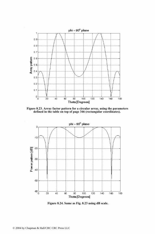
Fig.s 8.38 through 8.43 respectively show plots of the array gain pattern inthe U-V space, for the following cases:
[pattern] = rect_array(15, 15, 0.5, 0.5, 0, 0, -1, -1, -3) (8.73)
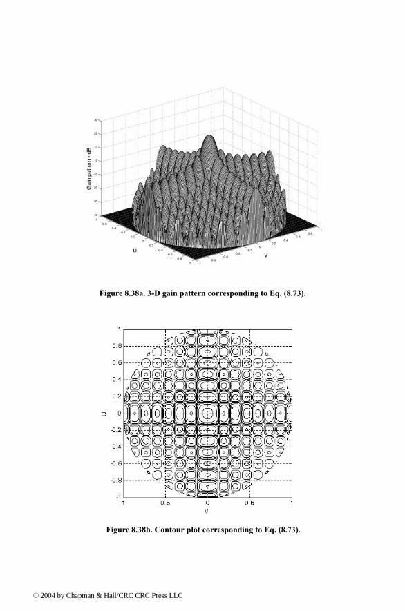
[pattern] = rect_array(15, 15, 0.5, 0.5, 20, 30, -1, -1, -3) (8.74)
[pattern] = rect_array(15, 15, 0.5, 0.5, 30, 30, 1, Hamming, -3) (8.75)
[pattern] = rect_array(15, 15, 0.5, 0.5, 30, 30, -1, -1, 3) (8.76)
[pattern] = rect_array(15, 15, 1, 0.5, 10, 30, -1, -1, -3) (8.77)
[pattern] = rect_array(15, 15, 1, 1, 0, 0, -1, -1, -3) (8.78)
1. This GUI was developed by Mr. David J. Hall, Consultant to Decibel Research, Inc., Huntsville, Alabama.
Figure 8.37. MATLAB GUI workspace array.m.
4 by Chapman & Hall/CRC CRC Press LLC
© 200
Figure 8.38a. 3-D gain pattern corresponding to Eq. (8.73).
Figure 8.38b. Contour plot corresponding to Eq. (8.73).
4 by Chapman & Hall/CRC CRC Press LLC
© 200
Figure 8.38c. Three-dimensional plot ( space) corresponding to Eq. (8.73).θ φ,
Figure 8.39a. 3-D gain pattern corresponding to Eq. (8.74).
4 by Chapman & Hall/CRC CRC Press LLC

© 200
Figure 8.39b. Contour plot corresponding to Eq. (8.74).
Figure 8.39c. 3-D plot ( space) corresponding to Eq. (8.74).θ φ,
4 by Chapman & Hall/CRC CRC Press LLC

© 200
Figure 8.40a. 3-D gain pattern corresponding to Eq. (8.75).
Figure 8.40b. Contour plot corresponding to Eq. (8.75).
4 by Chapman & Hall/CRC CRC Press LLC

© 200
Figure 8.41a. 3-D gain pattern corresponding to Eq. (8.76).
Figure 8.41b. Contour plot corresponding to Eq. (8.76).
4 by Chapman & Hall/CRC CRC Press LLC

© 200
Figure 8.41c. 3-D plot ( space) corresponding to Eq. (8.76).θ φ,
Figure 8.42a. 3-D gain pattern corresponding to Eq. (8.77).
4 by Chapman & Hall/CRC CRC Press LLC

© 200
Figure 8.42b. Contour plot corresponding to Eq. (8.77).
Figure 8.42c. 3-D plot ( space) corresponding to Eq. (8.77).θ φ,
4 by Chapman & Hall/CRC CRC Press LLC

© 200
Figure 8.43a. 3-D gain pattern corresponding to Eq. (8.78).
Figure 8.43b. Contour plot corresponding to Eq. (8.78).
4 by Chapman & Hall/CRC CRC Press LLC

© 200
MATLAB Function circ_array.m
The function circ_array.m computes and plots the rectangular grid with acircular array boundary antenna gain pattern in the visible U,V space. Thisfunction is given in Listing 8.6 in Section 8.8. The syntax is as follows:
[pattern, amn] = circ_array(N, dolxr, dolyr, theta0, phi0, winid, win, nbits);
where
Symbol Description Units Status
N number of elements along diameter none input
dolxr element spacing in lambda units along x wavelengths input
dolyr element spacing in lambda units along y wavelengths input
theta0 elevation steering angle degrees input
phi0 azimuth steering angle degrees input
winid -1: No weighting is used
1: Use weighting defined in win
none input
Figure 8.43c. 3-D plot ( space) corresponding to Eq. (8.78).θ φ,
4 by Chapman & Hall/CRC CRC Press LLC

© 200
Figs. 8.44 through 8.49 respectively show plots of the array gain pattern ver-sus steering for the following cases:
[pattern, amn] = circ_array(15, 0.5, 0.5, 0, 0, -1, -1, -3) (8.79)
[pattern, amn] = circ_array(15, 0.5, 0.5, 20, 30, -1, -1, -3) (8.80)
[pattern, amn] = circ_array(15, 0.5, 0.5, 30, 30, 1, Hamming, -3) (8.81)
[pattern, amn] = circ_array(15, 0.5, 0.5, 30, 30, -1, -1, 3) (8.82)
[pattern, amn] = circ_array(15, 1, 0.5, 10, 30, -1, -1, -3) (8.83)
[pattern, amn] = circ_array(15, 1, 1, 0, 0, -1, -1, -3) (8.84)
Note the function circ_array.m uses the function rec_to_circ.m, whichcomputes the array . It is given in Listing 8.7 in Section 8.8.
The MATLAB GUI workspace defined in array.m can be used to executethis function.
win window for sidelobe control none input
nbits negative #: perfect quantization
positive #: use quantization levels
none input
patterng gain pattern dB output
amn a(m,n) sequence defined in Eq. (8.68) none output
Symbol Description Units Status
2nbits
a m n,( )
4 by Chapman & Hall/CRC CRC Press LLC

© 200
Figure 8.44a. 3-D gain pattern corresponding to Eq. (8.79).
Figure 8.44b. Contour plot corresponding to Eq. (8.79).
4 by Chapman & Hall/CRC CRC Press LLC

© 200
Figure 8.44c. 3-D plot ( space) corresponding to Eq. (8.79).θ φ,
Figure 8.45a. 3-D gain pattern corresponding to Eq. (8.80).
4 by Chapman & Hall/CRC CRC Press LLC

© 200
Figure 8.45b. Contour plot corresponding to Eq. (8.80).
Figure 8.45c. 3-D plot ( space) corresponding to Eq. (8.80).θ φ,
4 by Chapman & Hall/CRC CRC Press LLC

© 200
Figure 8.46a. 3-D gain pattern corresponding to Eq. (8.81).
Figure 8.46b. Contour plot corresponding to Eq. (8.81).
4 by Chapman & Hall/CRC CRC Press LLC

© 200
Figure 8.47a. 3-D gain pattern corresponding to Eq. (8.82).
Figure 8.47b. Contour plot corresponding to Eq. (8.82).
4 by Chapman & Hall/CRC CRC Press LLC

© 200
Figure 8.47c. 3-D plot ( space) corresponding to Eq. (8.82).θ φ,
Figure 8.48a. 3-D gain pattern corresponding to Eq. (8.83).
4 by Chapman & Hall/CRC CRC Press LLC

© 200
Figure 8.48b. Contour plot corresponding to Eq. (8.83).
Figure 8.48c. 3-D plot ( space) corresponding to Eq. (8.83).θ φ,
4 by Chapman & Hall/CRC CRC Press LLC

© 200
Figure 8.49a. 3-D gain pattern corresponding to Eq. (8.84).
Figure 8.49b. Contour plot corresponding to Eq. (8.84).
4 by Chapman & Hall/CRC CRC Press LLC

© 200
The program array.m also plots the arrays element spacing pattern. Figs.8.50a and 8.50b show two examples. The xs indicate the location of actualactive array elements, while the os indicate the location of dummy or virtualelements created merely for computational purposes. More precisely, Fig.8.50a shows a rectangular grid with circular boundary as defined in Eqs. (8.67)and (8.68) with and . Fig. 8.50b shows a similarconfiguration except that an element spacing and .
8.6. Array Scan LossPhased arrays experience gain loss when the beam is steered away from the
array boresight, or zenith (normal to the face of the array). This loss is due tothe fact that the array effective aperture becomes smaller and consequently thearray beamwidth is broadened, as illustrated in Fig. 8.51. This loss in antennagain is called scan loss, , where
(8.85)
is effective aperture area at scan angle , and is effective array gain atthe same angle.
Figure 8.49c. 3-D plot ( space) corresponding to Eq. (8.84).θ φ,
dx dy 0.5λ= = a 0.35λ=dx 1.5λ= dy 0.5λ=
Lscan
LscanAAθ------ 2 G
Gθ------ 2
= =
Aθ θ Gθ
4 by Chapman & Hall/CRC CRC Press LLC

© 200
Figure 8.50a. A 15 element circular array made from a rectangular array with circular boundary. Element spacing .dx 0.5λ dy= =
Figure 8.50b. A 15 element circular array made from a rectangular array with circular boundary. Element spacing and .dy 0.5λ= dx 1.5λ=
4 by Chapman & Hall/CRC CRC Press LLC

© 200
The beamwidth at scan angle is
(8.86)
due to the increased scan loss at large scanning angles. In order to limit thescan loss to under some acceptable practical values, most arrays do not scanelectronically beyond about . Such arrays are called Full Field OfView (FFOV). FFOV arrays employ element spacing of or less to avoidgrating lobes. FFOV array scan loss is approximated by
(8.87)
Arrays that limit electronic scanning to under are referred to asLimited Field of View (LFOV) arrays. In this case the scan loss is
(8.88)
Fig. 8.52 shows a plot for scan loss versus scan angle. This figure can be repro-duced using MATLAB program fig8_52.m given in Listing 8.8.
maximum effective aperture
array boresight
effective aperture is reduced
effectiveaperture
effectiveaperture
Figure 8.51. Reduction in array effective aperture due to electronic scanning.
plane containingthe array
steeringangle
θ
ΘθΘbroadside
θcos------------------------=
θ 60°=0.6λ
Lscan θcos( )2.5≈
θ 60°=
Lscan
πdλ
------ θsin sin
πdλ
------ θsin-------------------------------
4
=
4 by Chapman & Hall/CRC CRC Press LLC

© 200
8.7. MyRadar Design Case Study - Visit 8
8.7.1. Problem Statement
Modify the MyRadar design case study such that we employ a phasedarray antenna. For this purpose, modify the design requirements such that thesearch volume is now defined by and . Assume X-band, ifpossible. Design an electronically steered radar (ESR). Non-coherent integra-tion of a few pulses may be used, if necessary. Size the radar so that it can ful-fill this mission. Calculate the antenna gain, aperture size, missile and aircraftdetection range, number of elements in the array, etc. All other design require-ments are as defined in the previous chapters.
8.7.2. A Design
The search volume is
(8.89)
Figure 8.52. Scan loss versus scan angle, based on Eq. (8.87).
Θe 10°= Θa 45°≤
Ω 10° 45°×
57.296( )2----------------------- 0.1371 steradian= =
4 by Chapman & Hall/CRC CRC Press LLC

© 200
For an X-band radar, choose , then
(8.90)
Assume an aperture size ; thus
(8.91)
Assume square aperture. It follows that the aperture 3-dB beamwidth is cal-culated from
(8.92)
The number of beams required to fill the search volume is
(8.93)
Note that the packing factor is used to allow for beam overlap in order toavoid gaps in the beam coverage. The search scan rate is 2 seconds. Thus, theminimum PRF should correspond to 200 beams per second (i.e., ).This PRF will allow the radar to visit each beam position only once during acomplete scan.
It was determined in Chapter 2 that 4-pulse non-coherent integration alongwith a cumulative detection scheme are required to achieve the desired proba-bility of detection. It was also determined that the single pulse energy for themissile and aircraft cases are respectively given by (see page 118)
(8.94)
(8.95)
However, these values were derived using and . Thenew wavelength is and the new gain is . Thus,the missile and aircraft single pulse energy, assuming the same single pulseSNR as derived in Chapter 2 (i.e., ) are
(8.96)
fo 9GHz=
λ 3 108×
9 109×----------------- 0.0333m= =
Ae 2.25m2=
G4πAe
λ2------------ 4 π 2.25××
0.0333( )2----------------------------- 25451.991 G⇒ 44dB= = = =
G 4πθ3db
2----------=
θ3dB⇒ 4 π 1802××
25451.991 π2×------------------------------------- 1.3°= =
nb kpΩ
1.3 57.296⁄( )2-----------------------------------
kp 1.5=
nb⇒ 399.5 choose nb⇒ 400= = =
kp
fr 200Hz=
Em 0.1147Joules=
Ea 0.1029Joules=
λ 0.1m= G 2827.4=λ 0.0333m= G 25451.99=
SNR 4dB=
Em 0.1147 0.12 2827.42×
0.03332 254522×------------------------------------------× 0.012765Joules= =
4 by Chapman & Hall/CRC CRC Press LLC

© 200
(8.97)
The single pulse peak power that will satisfy detection for both target typesis
(8.98)
where is used.
Note that since a 4-pulse non-coherent integration is adopted, the minimumPRF is increased to
(8.99)
and the total number of beams is . Consequently the unambiguousrange is
(8.100)
(1.101)
Since the effective aperture is , then by assuming an array effi-
ciency the actual array size is
(8.102)
It follows that the physical array sides are . Thus, by selectingthe array element spacing an array of size elements satis-fies the design requirements.
Since the field of view is less than , one can use element spacing aslarge as without introducing any grating lobes into the array FOV.Using this option yields an array of size elements. Hence, therequired power per element is less than .
8.8. MATLAB Program and Function ListingsThis section contains listings of all MATLAB programs and functions used
in this chapter. Users are encouraged to rerun this code with different inputs inorder to enhance their understanding of the theory.
Ea 0.1029 0.12 2827.42×
0.03332 254522×------------------------------------------× 0.01145Joules= =
Pt0.01276520 10 6×---------------------- 638.25W= =
τ 20µs=
fr 200 4× 800Hz= =
nb 1600=
Ru3 108×2 800×------------------≤ 187.5Km=
Ae 2.25m2=
ρ 0.8=
A 2.250.8---------- 2.8125m2= =
1.68m 1.68m×d 0.6λ= 84 84×
22.5°±d 1.5λ=
34 34× 1156=0.6W
4 by Chapman & Hall/CRC CRC Press LLC

© 200
Listing 8.1. MATLAB Program fig8_5.m% Use this code to produce figure 8.5a and 8.5b based on equation 8.34clear allclose alleps = 0.00001;k = 2*pi;theta = -pi : pi / 10791 : pi;var = sin(theta);nelements = 8;d = 1; % d = 1;num = sin((nelements * k * d * 0.5) .* var);
if(abs(num) <= eps) num = eps;endden = sin((k* d * 0.5) .* var);if(abs(den) <= eps) den = eps;end
pattern = abs(num ./ den);maxval = max(pattern);pattern = pattern ./ maxval;
figure(1)plot(var,pattern)xlabel('sine angle - dimensionless')ylabel('Array pattern')grid
figure(2)plot(var,20*log10(pattern))axis ([-1 1 -60 0])xlabel('sine angle - dimensionless')ylabel('Power pattern [dB]')grid;
figure(3)theta = theta +pi/2;polar(theta,pattern)title ('Array pattern')
figure(4)
4 by Chapman & Hall/CRC CRC Press LLC

© 200
polardb(theta,pattern)title ('Power pattern [dB]')
Listing 8.2. MATLAB Program fig8_7.m% Use this program to reproduce Fig. 8.7 of textclear allclose alleps =0.00001;N = 32;rect(1:32) = 1;ham = hamming(32);han = hanning(32);blk = blackman(32);k3 = kaiser(32,3);k6 = kaiser(32,6);RECT = 20*log10(abs(fftshift(fft(rect, 512)))./32 +eps);HAM = 20*log10(abs(fftshift(fft(ham, 512)))./32 +eps);HAN = 20*log10(abs(fftshift(fft(han, 512)))./32+eps);BLK = 20*log10(abs(fftshift(fft(blk, 512)))./32+eps);K6 = 20*log10(abs(fftshift(fft(k6, 512)))./32+eps);x = linspace(-1,1,512);figuresubplot(2,1,1)plot(x,RECT,'k--',x,HAM,'k',x,HAN,'k-.');xlabel('x')ylabel('Window')gridaxis tightlegend('Rectangular','Hamming','Hanning')subplot(2,1,2)plot(x,RECT,'k--',x,BLK,'k',x,K6,'K-.')xlabel('x')ylabel('Window')legend('Rectangular','Blackman','Kasier at \beta = 6')gridaxis tight
Listing 8.3. MATLAB Function linear_array.mfunction [theta,patternr,patterng] = linear_array(Nr,dolr,theta0,winid,win,nbits);% This function computes and returns the gain radiation pattern for a linear array
4 by Chapman & Hall/CRC CRC Press LLC

© 200
% It uses the FFT to compute the pattern%%%%%%%%% ********** INPUTS *********** %%%%%%%%%%% Nr ==> number of elements; dolr ==> element spacing (d) in lambda units divided by lambda% theta0 ==> steering angle in degrees; winid ==> use winid negative for no window, winid positive to enter your window of size(Nr)% win is input window, NOTE that win must be an NrX1 row vector; nbits ==> number of bits used in the phase shifters% negative nbits mean no quantization is used%%%%%% *********** OUTPUTS *********** %%%%%%%%%%%%% theta ==> real-space angle; patternr ==> array radiation pattern in dBs% patterng ==> array directive gain pattern in dBs%%%%%%%%%%%% **************** %%%%%%%%%%%%eps = 0.00001;n = 0:Nr-1;i = sqrt(-1);%if dolr is > 0.5 then; choose dol = 0.25 and compute new Nif(dolr <=0.5) dol = dolr; N = Nr;else ratio = ceil(dolr/.25); N = Nr * ratio; dol = 0.25;end% choose proper size fft, for minimum value choose 256Nrx = 10 * N; nfft = 2^(ceil(log(Nrx)/log(2)));if nfft < 256 nfft = 256;end% convert steering angle into radians; and compute the sine of angletheta0 = theta0 *pi /180.;sintheta0 = sin(theta0);% determine and compute quantized steering angleif nbits < 0 phase0 = exp(i*2.0*pi .* n * dolr * sintheta0);else % compute and add the phase shift terms (WITH nbits quantization) % Use formula thetal = (2*pi*n*dol) * sin(theta0) divided into 2^nbits % and rounded to the nearest qunatization level levels = 2^nbits; qlevels = 2.0 * pi / levels; % compute quantization levels
4 by Chapman & Hall/CRC CRC Press LLC

© 200
% compute the phase level and round it to the closest quantization level at each array element angleq = round(dolr .* n * sintheta0 * levels) .* qlevels; % vector of possi-ble angles phase0 = exp(i*angleq);end% generate array of elements with or without windowif winid < 0 wr(1:Nr) = 1;else wr = win';end% add the phase shift terms wr = wr .* phase0; % determine if interpolation is needed (i.e., N > Nr)if N > Nr w(1:N) = 0; w(1:ratio:N) = wr(1:Nr);else w = wr;end% compute the sine(theta) in real space that corresponds to the FFT index arg = [-nfft/2:(nfft/2)-1] ./ (nfft*dol);idx = find(abs(arg) <= 1);sinetheta = arg(idx);theta = asin(sinetheta);% convert angle into degreestheta = theta .* (180.0 / pi);% Compute fft of w (radiation pattern)patternv = (abs(fftshift(fft(w,nfft)))).^2;% convert radiationa pattern to dBspatternr = 10*log10(patternv(idx) ./Nr + eps);% Compute directive gain pattern rbarr = 0.5 *sum(patternv(idx)) ./ (nfft * dol);patterng = 10*log10(patternv(idx) + eps) - 10*log10(rbarr + eps);return
Listing 8.4. MATLAB Program circular_array.m% Circular Array in the x-y plane % Element is a short dipole antenna parallel to the z axis% 2D Radiation Patterns for fixed phi or fixed theta% dB polar plots uses the polardb.m file% Last modified: July 13, 2003
4 by Chapman & Hall/CRC CRC Press LLC

© 200
%%%%% Element expression needs to be modified if different%%%% than a short dipole antenna along the z axisclear allclf% close all% ==== Input Parameters ====a = 1.; % radius of the circleN = 20; % number of Elements of the circular arraytheta0 = 45; % main beam Theta directionphi0 = 60; % main beam Phi direction% Theta or Phi variations for the calculations of the far field patternVariations = 'Phi'; % Correct selections are 'Theta' or 'Phi' phid = 60; % constant phi plane for theta variationsthetad = 45; % constant theta plane for phi variations% ==== End of Input parameters section ====dtr = pi/180; % conversion factorsrtd = 180/pi;phi0r = phi0*dtr;theta0r = theta0*dtr;lambda = 1; k = 2*pi/lambda;ka = k*a; % Wavenumber times the radiusjka = j*ka;I(1:N) = 1; % Elements excitation Amplitude and Phasealpha(1:N) =0; for n = 1:N % Element positions Uniformly distributed along the circle phin(n) = 2*pi*n/N;endswitch Variationscase 'Theta' phir = phid*dtr; % Pattern in a constant Phi plane i = 0; for theta = 0.001:1:181 i = i+1; thetar(i) = theta*dtr; angled(i) = theta; angler(i) = thetar(i); Arrayfactor(i) = 0; for n = 1:N Arrayfactor(i) = Arrayfactor(i) + I(n)*exp(j*alpha(n)) ... * exp( jka*(sin(thetar(i))*cos(phir -phin(n))) ... -jka*(sin(theta0r )*cos(phi0r-phin(n))) ); end Arrayfactor(i) = abs(Arrayfactor(i));
4 by Chapman & Hall/CRC CRC Press LLC

© 200
Element(i) = abs(sin(thetar(i)+0*dtr)); % use the abs function to avoid endcase 'Phi' thetar = thetad*dtr; % Pattern in a constant Theta plane i = 0; for phi = 0.001:1:361 i = i+1; phir(i) = phi*dtr; angled(i) = phi; angler(i) = phir(i); Arrayfactor(i) = 0; for n = 1:N Arrayfactor(i) = Arrayfactor(i) + I(n)*exp(j*alpha(n)) ... * exp( jka*(sin(thetar )*cos(phir(i)-phin(n))) ... -jka*(sin(theta0r)*cos(phi0r -phin(n))) ); end Arrayfactor(i) = abs(Arrayfactor(i)); Element(i) = abs(sin(thetar+0*dtr)); % use the abs function to avoid end endangler = angled*dtr;Element = Element/max(Element);Array = Arrayfactor/max(Arrayfactor);ArraydB = 20*log10(Array);EtotalR =(Element.*Arrayfactor)/max(Element.*Arrayfactor);figure(1)plot(angled,Array)ylabel('Array pattern')gridswitch Variationscase 'Theta' axis ([0 180 0 1 ])% theta = theta +pi/2; xlabel('Theta [Degrees]') title ( 'phi = 90^o plane')case 'Phi'axis ([0 360 0 1 ]) xlabel('Phi [Degrees]') title ( 'Theta = 90^o plane')endfigure(2)plot(angled,ArraydB)%axis ([-1 1 -60 0])ylabel('Power pattern [dB]')grid;
4 by Chapman & Hall/CRC CRC Press LLC

© 200
switch Variationscase 'Theta' axis ([0 180 -60 0 ]) xlabel('Theta [Degrees]') title ( 'phi = 90^o plane')case 'Phi'axis ([0 360 -60 0 ]) xlabel('Phi [Degrees]') title ( 'Theta = 90^o plane')endfigure(3)polar(angler,Array)title ('Array pattern')figure(4)polardb(angler,Array)title ('Power pattern [dB]')% the plots provided above are for the array factor based on the circular % array plots for other patterns such as those for the antenna element % (Element)or the total pattern (Etotal based on Element*Arrayfactor) can % also be displayed by the user as all these patterns are already computed % above.figure(10)subplot(2,2,1) polardb (angler,Element,'b-'); % rectangular plot of element patterntitle('Element normalized E field [dB]')subplot(2,2,2)polardb(angler,Array,'b-')title(' Array Factor normalized [dB]')subplot(2,2,3)polardb(angler,EtotalR,'b-'); % polar plottitle('Total normalized E field [dB]')%%%%%%%%%%%%%%%%%%%%%%%%%%%%%%%%%%%%%%%%%%%%%%%%%%%%function polardb(theta,rho,line_style)% POLARDB Polar coordinate plot.% POLARDB(THETA, RHO) makes a plot using polar coordinates of% the angle THETA, in radians, versus the radius RHO in dB.% The maximum value of RHO should not exceed 1. It should not be% normalized, however (i.e., its max. value may be less than 1).% POLAR(THETA,RHO,S) uses the linestyle specified in string S.% See PLOT for a description of legal linestyles.if nargin < 1 error('Requires 2 or 3 input arguments.')elseif nargin == 2
4 by Chapman & Hall/CRC CRC Press LLC

© 200
if isstr(rho) line_style = rho; rho = theta; [mr,nr] = size(rho); if mr == 1 theta = 1:nr; else th = (1:mr)'; theta = th(:,ones(1,nr)); end else line_style = 'auto'; endelseif nargin == 1 line_style = 'auto'; rho = theta; [mr,nr] = size(rho); if mr == 1 theta = 1:nr; else th = (1:mr)'; theta = th(:,ones(1,nr)); endendif isstr(theta) | isstr(rho) error('Input arguments must be numeric.');endif ~isequal(size(theta),size(rho)) error('THETA and RHO must be the same size.');end% get hold statecax = newplot;next = lower(get(cax,'NextPlot'));hold_state = ishold;
% get x-axis text color so grid is in same colortc = get(cax,'xcolor');ls = get(cax,'gridlinestyle');% Hold on to current Text defaults, reset them to the% Axes' font attributes so tick marks use them.fAngle = get(cax, 'DefaultTextFontAngle');fName = get(cax, 'DefaultTextFontName');fSize = get(cax, 'DefaultTextFontSize');fWeight = get(cax, 'DefaultTextFontWeight');
4 by Chapman & Hall/CRC CRC Press LLC

© 200
fUnits = get(cax, 'DefaultTextUnits');set(cax, 'DefaultTextFontAngle', get(cax, 'FontAngle'), ... 'DefaultTextFontName', get(cax, 'FontName'), ... 'DefaultTextFontSize', get(cax, 'FontSize'), ... 'DefaultTextFontWeight', get(cax, 'FontWeight'), ... 'DefaultTextUnits','data')% make a radial grid hold on; maxrho =1; hhh=plot([-maxrho -maxrho maxrho maxrho],[-maxrho maxrho maxrho -maxrho]); set(gca,'dataaspectratio',[1 1 1],'plotboxaspectratiomode','auto') v = [get(cax,'xlim') get(cax,'ylim')]; ticks = sum(get(cax,'ytick')>=0); delete(hhh);% check radial limits and ticks rmin = 0; rmax = v(4); rticks = max(ticks-1,2); if rticks > 5 % see if we can reduce the number if rem(rticks,2) == 0 rticks = rticks/2; elseif rem(rticks,3) == 0 rticks = rticks/3; end end% only do grids if hold is offif ~hold_state% define a circle th = 0:pi/50:2*pi; xunit = cos(th); yunit = sin(th);% now really force points on x/y axes to lie on them exactly inds = 1:(length(th)-1)/4:length(th); xunit(inds(2:2:4)) = zeros(2,1); yunit(inds(1:2:5)) = zeros(3,1);% plot background if necessary if ~isstr(get(cax,'color')), patch('xdata',xunit*rmax,'ydata',yunit*rmax, ... 'edgecolor',tc,'facecolor',get(gca,'color'),... 'handlevisibility','off'); end% draw radial circles with dB ticks c82 = cos(82*pi/180); s82 = sin(82*pi/180); rinc = (rmax-rmin)/rticks;
4 by Chapman & Hall/CRC CRC Press LLC

© 200
tickdB=-10*(rticks-1); % the innermost tick dB value for i=(rmin+rinc):rinc:rmax hhh = plot(xunit*i,yunit*i,ls,'color',tc,'linewidth',1,... 'handlevisibility','off'); text((i+rinc/20)*c82*0,-(i+rinc/20)*s82, ... [' ' num2str(tickdB) ' dB'],'verticalalignment','bottom',... 'handlevisibility','off') tickdB=tickdB+10; end set(hhh,'linestyle','-') % Make outer circle solid% plot spokes th = (1:6)*2*pi/12; cst = cos(th); snt = sin(th); cs = [-cst; cst]; sn = [-snt; snt]; plot(rmax*cs,rmax*sn,ls,'color',tc,'linewidth',1,... 'handlevisibility','off')% annotate spokes in degrees rt = 1.1*rmax; for i = 1:length(th) text(rt*cst(i),rt*snt(i),int2str(i*30),... 'horizontalalignment','center',... 'handlevisibility','off'); if i == length(th) loc = int2str(0); else loc = int2str(180+i*30); end text(-rt*cst(i),-rt*snt(i),loc,'horizontalalignment','center',... 'handlevisibility','off') end% set view to 2-D view(2);% set axis limits axis(rmax*[-1 1 -1.15 1.15]);end% Reset defaults.set(cax, 'DefaultTextFontAngle', fAngle , ... 'DefaultTextFontName', fName , ... 'DefaultTextFontSize', fSize, ... 'DefaultTextFontWeight', fWeight, ... 'DefaultTextUnits', fUnits );% Transfrom data to dB scalermin = 0; rmax=1;
4 by Chapman & Hall/CRC CRC Press LLC

© 200
rinc = (rmax-rmin)/rticks;rhodb=zeros(1,length(rho));for i=1:length(rho) if rho(i)==0 rhodb(i)=0; else rhodb(i)=rmax+2*log10(rho(i))*rinc; end if rhodb(i)<=0 rhodb(i)=0; endend% transform data to Cartesian coordinates.xx = rhodb.*cos(theta);yy = rhodb.*sin(theta);% plot data on top of gridif strcmp(line_style,'auto') q = plot(xx,yy);else q = plot(xx,yy,line_style);endif nargout > 0 hpol = q;endif ~hold_state set(gca,'dataaspectratio',[1 1 1]), axis off; set(cax,'NextPlot',next);endset(get(gca,'xlabel'),'visible','on')set(get(gca,'ylabel'),'visible','on')
Listing 8.5. MATLAB Function rect_array.mfunction [pattern] = rect_array(Nxr,Nyr,dolxr,dolyr,theta0,phi0,winid,win,nbits);%%%%%%%%%% ************************ %%%%%%%%%%% This function computes the 3-D directive gain patterns for a planar array% This function uses the fft2 to compute its output%%%%%%%% ************ INPUTS ************ %%%%%%%%%% Nxr ==> number of along x-axis; Nyr ==> number of elements along y-axis% dolxr ==> element spacing in x-direction; dolyr ==> element spacing in y-direction Both are in lambda units% theta0 ==> elevation steering angle in degrees, phi0 ==> azimuth steering angle in degrees
4 by Chapman & Hall/CRC CRC Press LLC

© 200
% winid ==> window identifier; winid negative ==> no window ; winid posi-tive ==> use window given by win% win ==> input window function (2-D window) MUST be of size (Nxr X Nyr)% nbits is the number of nbits used in phase quantization; nbits negative ==> NO quantization%%%%% *********** OUTPUTS ************* %%%%%%%% pattern ==> directive gain pattern%%%%%%% ************************ %%%%%%%%%%%%eps = 0.0001;nx = 0:Nxr-1;ny = 0:Nyr-1;i = sqrt(-1);% check that window size is the same as the array size[nw,mw] = size(win);if winid >0 if nw ~= Nxr fprintf('STOP == Window size must be the same as the array') returnendif mw ~= Nyr fprintf('STOP == Window size must be the same as the array') returnendend
%if dol is > 0.5 then; choose dol = 0.5 and compute new Nif(dolxr <=0.5) ratiox = 1 ; dolx = dolxr ; Nx = Nxr ;else ratiox = ceil(dolxr/.5) ; Nx = (Nxr -1 ) * ratiox + 1 ; dolx = 0.5 ;endif(dolyr <=0.5) ratioy = 1 ; doly = dolyr ; Ny = Nyr ;else ratioy = ceil(dolyr/.5) ; Ny = (Nyr -1) * ratioy + 1 ; doly = 0.5 ;end
4 by Chapman & Hall/CRC CRC Press LLC

© 200
% choose proper size fft, for minimum value choose 256X256Nrx = 10 * Nx; Nry = 10 * Ny;nfftx = 2^(ceil(log(Nrx)/log(2)));nffty = 2^(ceil(log(Nry)/log(2)));if nfftx < 256 nfftx = 256;endif nffty < 256 nffty = 256;end% generate array of elements with or without windowif winid < 0 array = ones(Nxr,Nyr);else array = win;end% convert steering angles (theta0, phi0) to radianstheta0 = theta0 * pi / 180;phi0 = phi0 * pi / 180;% convert steering angles (theta0, phi0) to U-V sine-spaceu0 = sin(theta0) * cos(phi0);v0 = sin(theta0) * sin(phi0);% Use formula thetal = (2*pi*n*dol) * sin(theta0) divided into 2^m levels% and rounded to the nearest qunatization levelif nbits < 0 phasem = exp(i*2*pi*dolx*u0 .* nx *ratiox); phasen = exp(i*2*pi*doly*v0 .* ny *ratioy);else levels = 2^nbits; qlevels = 2.0*pi / levels; % compute quantization levels sinthetaq = round(dolx .* nx * u0 * levels * ratiox) .* qlevels; % vector of possible angles sinphiq = round(doly .* ny * v0 * levels *ratioy) .* qlevels; % vector of pos-sible angles phasem = exp(i*sinthetaq); phasen = exp(i*sinphiq); end% add the phase shift termsarray = array .* (transpose(phasem) * phasen);% determine if interpolation is needed (i.e., N > Nr)if (Nx > Nxr )| (Ny > Nyr) for xloop = 1 : Nxr temprow = array(xloop, :) ;
4 by Chapman & Hall/CRC CRC Press LLC

© 200
w( (xloop-1)*ratiox+1, 1:ratioy:Ny) = temprow ; end array = w;else w = array ;% w(1:Nx, :) = array(1:N,:);end% Compute array patternarrayfft = abs(fftshift(fft2(w,nfftx,nffty))).^2 ;%compute [su,sv] matrixU = [-nfftx/2:(nfftx/2)-1] ./(dolx*nfftx);indexx = find(abs(U) <= 1);U = U(indexx);V = [-nffty/2:(nffty/2)-1] ./(doly*nffty);indexy = find(abs(V) <= 1);V = V(indexy);%Normalize to generate gain paternrbar=sum(sum(arrayfft(indexx,indexy))) / dolx/doly/4./nfftx/nffty;arrayfft = arrayfft(indexx,indexy) ./rbar;[SU,SV] = meshgrid(V,U);indx = find((SU.^2 + SV.^2) >1);arrayfft(indx) = eps/10;pattern = 10*log10(arrayfft +eps);figure(1)mesh(V,U,pattern);xlabel('V')ylabel('U');zlabel('Gain pattern - dB')figure(2)contour(V,U,pattern)gridaxis imagexlabel('V')ylabel('U');axis([-1 1 -1 1])figure(3)x0 = (Nx+1)/2 ;y0 = (Ny+1)/2 ;radiusx = dolx*((Nx-1)/2) ;radiusy = doly*((Ny-1)/2) ;[xxx, yyy]=find(abs(array)>eps);xxx = xxx-x0 ;yyy = yyy-y0 ;plot(yyy*doly, xxx*dolx,'rx')
4 by Chapman & Hall/CRC CRC Press LLC

© 200
hold onaxis([-radiusy-0.5 radiusy+0.5 -radiusx-0.5 radiusx+0.5]);gridtitle('antenna spacing pattern');xlabel('y - \lambda units')ylabel('x - \lambda units')[xxx0, yyy0]=find(abs(array)<=eps);xxx0 = xxx0-x0 ;yyy0 = yyy0-y0 ;plot(yyy0*doly, xxx0*dolx,'co')axis([-radiusy-0.5 radiusy+0.5 -radiusx-0.5 radiusx+0.5]);hold offreturn
Listing 8.6. MATLAB Function circ_array.mfunction [pattern,amn] = circ_array(N,dolxr,dolyr,theta0,phi0,winid,win,nbits);%%%%%%%%% ************************ %%%%%%%%%%%% This function computes the 3-D directive gain patterns for a circular planar array% This function uses the fft2 to compute its output. It assumes that there are the same number of elements along the major x- and y-axes%%%%%%%% ************ INPUTS ************ %%%%%%%%% N ==> number of elements along x-aixs or y-axis% dolxr ==> element spacing in x-direction; dolyr ==> element spacing in y-direction. Both are in lambda units% theta0 ==> elevation steering angle in degrees, phi0 ==> azimuth steering angle in degrees% This function uses the function (rec_to_circ) which computes the circular array from a square % array (of size NXN) using the notation developed by ALLEN,J.L.,"The The-ory of Array Antennas % (with Emphasis on Radar Application)" MIT-LL Technical Report No. 323, July, 25 1965. % winid ==> window identifier; winid negative ==> no window ; winid posi-tive ==> use window given by win% win ==> input window function (2-D window) MUST be of size (Nxr X Nyr)% nbits is the number of nbits used in phase quantization; nbits negative ==> NO quantization%%%%%%% *********** OUTPUTS ************* %%%%%%%%% amn ==> array of ones and zeros; ones indicate true element location on the grid% zeros mean no elements at that location; pattern ==> directive gain pattern
4 by Chapman & Hall/CRC CRC Press LLC

© 200
%%%%%%%%% ************************ %%%%%%%%%%%%eps = 0.0001;nx = 0:N-1;ny = 0:N-1;i = sqrt(-1);% check that window size is the same as the array size[nw,mw] = size(win);if winid >0 if mw ~= N fprintf('STOP == Window size must be the same as the array') return end if nw ~= N fprintf('STOP == Window size must be the same as the array') return endend%if dol is > 0.5 then; choose dol = 0.5 and compute new Nif(dolxr <=0.5) ratiox = 1 ; dolx = dolxr ; Nx = N ;else ratiox = ceil(dolxr/.5) ; Nx = (N-1) * ratiox + 1 ; dolx = 0.5 ;endif(dolyr <=0.5) ratioy = 1 ; doly = dolyr ; Ny = N ;else ratioy = ceil(dolyr/.5); Ny = (N-1)*ratioy + 1 ; doly = 0.5 ;end% choose proper size fft, for minimum value choose 256X256Nrx = 10 * Nx; Nry = 10 * Ny;nfftx = 2^(ceil(log(Nrx)/log(2)));nffty = 2^(ceil(log(Nry)/log(2)));if nfftx < 256 nfftx = 256;end
4 by Chapman & Hall/CRC CRC Press LLC

© 200
if nffty < 256 nffty = 256;end% generate array of elements with or without windowif winid < 0 array = ones(N,N);else array = win;end% convert steering angles (theta0, phi0) to radianstheta0 = theta0 * pi / 180;phi0 = phi0 * pi / 180;% convert steering angles (theta0, phi0) to U-V sine-spaceu0 = sin(theta0) * cos(phi0);v0 = sin(theta0) * sin(phi0);% Use formula thetal = (2*pi*n*dol) * sin(theta0) divided into 2^m levels% and rounded to the nearest qunatization levelif nbits < 0 phasem = exp(i*2*pi*dolx*u0 .* nx * ratiox); phasen = exp(i*2*pi*doly*v0 .* ny * ratioy);else levels = 2^nbits; qlevels = 2.0*pi / levels; % compute quantization levels sinthetaq = round(dolx .* nx * u0 * levels * ratiox) .* qlevels; % vector of possible angles sinphiq = round(doly .* ny * v0 * levels *ratioy) .* qlevels; % vector of pos-sible angles phasem = exp(i*sinthetaq); phasen = exp(i*sinphiq); end% add the phase shift termsarray = array .* (transpose(phasem) * phasen) ;
% determine if interpolation is needed (i.e., N > Nr)if (Nx > N )| (Ny > N) for xloop = 1 : N temprow = array(xloop, :) ; w( (xloop-1)*ratiox+1, 1:ratioy:Ny) = temprow ; end array = w;else w(1:Nx, :) = array(1:N,:);end% Convert rectangular array into circular using function rec_to_circ
4 by Chapman & Hall/CRC CRC Press LLC

© 200
[m,n] = size(w) ;NC = max(m,n); % Use Allens algorithmif Nx == Ny temp_array = w;else midpoint = (NC-1)/2 +1 ; midwm = (m-1)/2 ; midwn = (n-1)/2 ; temp_array = zeros(NC,NC); temp_array(midpoint-midwm:midpoint+midwm, midpoint-midwn:mid-point+midwn) = w ;endamn = rec_to_circ(NC); % must be rectangular array (Nx=Ny)amn = temp_array .* amn ;
% Compute array patternarrayfft = abs(fftshift(fft2(amn,nfftx,nffty))).^2 ;%compute [su,sv] matrixU = [-nfftx/2:(nfftx/2)-1] ./(dolx*nfftx);indexx = find(abs(U) <= 1);U = U(indexx);V = [-nffty/2:(nffty/2)-1] ./(doly*nffty);indexy = find(abs(V) <= 1);V = V(indexy);[SU,SV] = meshgrid(V,U);indx = find((SU.^2 + SV.^2) >1);arrayfft(indx) = eps/10;%Normalize to generate gain patternrbar=sum(sum(arrayfft(indexx,indexy))) / dolx/doly/4./nfftx/nffty;arrayfft = arrayfft(indexx,indexy) ./rbar;[SU,SV] = meshgrid(V,U);indx = find((SU.^2 + SV.^2) >1);arrayfft(indx) = eps/10;pattern = 10*log10(arrayfft +eps);figure(1)mesh(V,U,pattern);xlabel('V')ylabel('U');zlabel('Gain pattern - dB')figure(2)contour(V,U,pattern)axis imagegridxlabel('V')
4 by Chapman & Hall/CRC CRC Press LLC

© 200
ylabel('U');axis([-1 1 -1 1])figure(3)x0 = (NC+1)/2 ;y0 = (NC+1)/2 ;radiusx = dolx*((NC-1)/2 + 0.05/dolx) ;radiusy = doly*((NC-1)/2 + 0.05/dolx) ;theta = 5 ;[xxx, yyy]=find(abs(amn)>0);xxx = xxx-x0 ;yyy = yyy-y0 ;plot(yyy*doly, xxx*dolx,'rx')axis equalhold onaxis([-radiusy-0.5 radiusy+0.5 -radiusx-0.5 radiusx+0.5]);gridtitle('antenna spacing pattern');xlabel('y - \lambda units')ylabel('x - \lambda units')[x, y]= makeellip( 0, 0, radiusx, radiusy, theta) ;plot(y, x) ;axis([-radiusy-0.5 radiusy+0.5 -radiusx-0.5 radiusx+0.5]);[xxx0, yyy0]=find(abs(amn)<=0);xxx0 = xxx0-x0 ;yyy0 = yyy0-y0 ;plot(yyy0*doly, xxx0*dolx,'co')axis([-radiusy-0.5 radiusy+0.5 -radiusx-0.5 radiusx+0.5]);axis equalhold off ;return
Listing 8.7. MATLAB Function rec_to_circ.mfunction amn = rec_to_circ(N)midpoint = (N-1)/2 + 1;amn = zeros(N);array1(midpoint,midpoint) = N;x0 = midpoint;y0 = x0;for i = 1:N for j = 1:N distance(i,j) = sqrt((x0-i)^2 + (y0-j)^2); endend
4 by Chapman & Hall/CRC CRC Press LLC

© 200
idx = find(distance < (N-1)/2 + .4);amn (idx) = 1;return
Listing 8.8. MATLAB Program fig8_52.m%Use this program to reproduce Fig. 8.40. Based on Eq. (8.87)clear allclose alld = 0.6; % element spacing in lambda unitsbetadeg = linspace(0,22.5,1000);beta = betadeg .*pi ./180;den = pi*d .* sin(beta);numarg = den;num = sin(numarg);lscan = (num./den).^-4;LSCAN = 10*log10(lscan+eps);figure (1)plot(betadeg,LSCAN)xlabel('scan angle in degrees')ylabel('Scan loss in dB')gridtitle('Element spacing is d = 0.6 \lambda ')
4 by Chapman & Hall/CRC CRC Press LLC
Related Documents