Essential Graduate Physics QM: Quantum Mechanics © K. Likharev Chapter 8. Multiparticle Systems This chapter provides a brief introduction to quantum mechanics of systems of similar particles, with special attention to the case when they are indistinguishable. For such systems, theory predicts (and experiment confirms) very specific effects even in the case of negligible explicit (“direct”) interactions between the particles. These effects notably include the Bose-Einstein condensation of bosons and the exchange interaction of fermions. 8.1. Distinguishable and indistinguishable particles The importance of quantum systems of many similar particles is probably self-evident; just the very fact that most atoms include several/many electrons is sufficient to attract our attention. There are also important systems where the total number of electrons is much higher than in one atom; for example, a cubic centimeter of a typical metal houses ~10 23 conduction electrons that cannot be attributed to particular atoms, and have to be considered as common parts of the system as the whole. Though quantum mechanics offers virtually no exact analytical results for systems of substantially interacting particles, 1 it reveals very important new quantum effects even in the simplest cases when particles do not interact, and least explicitly (directly). If non-interacting particles are either different from each other by their nature, or physically similar but still distinguishable because of other reasons, everything is simple – at least, conceptually. Then, as was already discussed in Sec. 6.7, a system of two particles, 1 and 2, each in a pure quantum state, may be described by a state vector which is a direct product, 2 1 ' , (8.1a) 1 As was emphasized in Sec. 7.3, for such systems of similar particles the powerful methods discussed in the last chapter, based on the separation of the whole Universe into a “system of our interest” and its “environment”, typically do not work well – mostly because the quantum state of the “particle of interest” may be substantially correlated (in particular, entangled) with those of similar particles forming its “environment” – see below. of single-particle vectors, describing their states and ’ defined in different Hilbert spaces. (Below, I will frequently use, for such direct product, the following convenient shorthand: ' , (8.1b) in which the particle’s number is coded by the state symbol’s position.) Hence the permuted state 2 1 ˆ ' ' ' P , (8.2) where P ˆ is the permutation operator defined by Eq. (2), is clearly different from the initial one. This operator may be also used for states of systems of identical particles. In physics, the last term may be used to describe: (i) the “really elementary” particles like electrons, which (at least at this stage of development of physics) are considered as structure-less entities, and hence are all identical; Distinguish- able particles

Welcome message from author
This document is posted to help you gain knowledge. Please leave a comment to let me know what you think about it! Share it to your friends and learn new things together.
Transcript
Essential Graduate Physics QM: Quantum Mechanics
© K. Likharev
Chapter 8. Multiparticle Systems
This chapter provides a brief introduction to quantum mechanics of systems of similar particles, with special attention to the case when they are indistinguishable. For such systems, theory predicts (and experiment confirms) very specific effects even in the case of negligible explicit (“direct”) interactions between the particles. These effects notably include the Bose-Einstein condensation of bosons and the exchange interaction of fermions.
8.1. Distinguishable and indistinguishable particles
The importance of quantum systems of many similar particles is probably self-evident; just the very fact that most atoms include several/many electrons is sufficient to attract our attention. There are also important systems where the total number of electrons is much higher than in one atom; for example, a cubic centimeter of a typical metal houses ~1023 conduction electrons that cannot be attributed to particular atoms, and have to be considered as common parts of the system as the whole. Though quantum mechanics offers virtually no exact analytical results for systems of substantially interacting particles,1 it reveals very important new quantum effects even in the simplest cases when particles do not interact, and least explicitly (directly).
If non-interacting particles are either different from each other by their nature, or physically similar but still distinguishable because of other reasons, everything is simple – at least, conceptually. Then, as was already discussed in Sec. 6.7, a system of two particles, 1 and 2, each in a pure quantum state, may be described by a state vector which is a direct product,
21
' , (8.1a)
1 As was emphasized in Sec. 7.3, for such systems of similar particles the powerful methods discussed in the last chapter, based on the separation of the whole Universe into a “system of our interest” and its “environment”, typically do not work well – mostly because the quantum state of the “particle of interest” may be substantially correlated (in particular, entangled) with those of similar particles forming its “environment” – see below.
of single-particle vectors, describing their states and ’ defined in different Hilbert spaces. (Below, I will frequently use, for such direct product, the following convenient shorthand:
' , (8.1b)
in which the particle’s number is coded by the state symbol’s position.) Hence the permuted state
21
ˆ '''P , (8.2)
where P is the permutation operator defined by Eq. (2), is clearly different from the initial one.
This operator may be also used for states of systems of identical particles. In physics, the last term may be used to describe:
(i) the “really elementary” particles like electrons, which (at least at this stage of development of physics) are considered as structure-less entities, and hence are all identical;
Distinguish- able
particles
Essential Graduate Physics QM: Quantum Mechanics
Chapter 8 Page 2 of 52
(ii) any objects (e.g., hadrons or mesons) that may be considered as a system of “more elementary” particles (e.g., quarks and gluons), but are placed in the same internal quantum state – most simply, though not necessarily, in the ground state.2
It is important to note that identical particles still may be distinguishable – say by their clear spatial separation. Such systems of similar but distinguishable particles (or subsystems) are broadly discussed nowadays in the context of quantum computing and encryption – see Sec. 5 below. This is why it is insufficient to use the term “identical particles” if we want to say that they are genuinely indistinguishable, so I below I will use the latter term, despite it being rather unpleasant grammatically.
It turns out that for a quantitative description of systems of indistinguishable particles we need to use, instead of direct products of the type (1), linear combinations of such products, for example of ’ and ’.3 To see this, let us discuss the properties of the permutation operator defined by Eq. (2). Consider an observable A, and a system of eigenstates of its operator:
jjj aAaA ˆ . (8.3)
If the particles are indistinguishable, the observable’s expectation value should not be affected by their
permutation. Hence the operators A and P have to commute and share their eigenstates. This is why
the eigenstates of the operator P are so important: in particular, they include the eigenstates of the
Hamiltonian, i.e. the stationary states of a system of indistinguishable particles.
Let us have a look at the action of the permutation operator squared, on an elementary ket-vector product:
'''' PPPP ˆˆˆˆ 2 , (8.4)
i.e. 2P brings the state back to its original form. Since any pure state of a two-particle system may be
represented as a linear combination of such products, this result does not depend on the state, and may be represented as the following operator relation:
.ˆ 2 IP (8.5)
Now let us find the possible eigenvalues Pj of the permutation operator. Acting by both sides of Eq. (5)
on any of eigenstates j of the permutation operator, we get a very simple equation for its eigenvalues:
12 jP , (8.6)
2 Note that from this point of view, even complex atoms or molecules, in the same internal quantum state, may be considered on the same footing as the “really elementary” particles. For example, the already mentioned recent spectacular interference experiments by R. Lopes et al., which require particle identity, were carried out with couples of 4He atoms in the same internal quantum state. 3 A very legitimate question is why, in this situation, we need to introduce the particles’ numbers to start with. A partial answer is that in this approach, it is much simpler to derive (or guess) the system Hamiltonians from the correspondence principle – see, e.g., Eq. (27) below. Later in this chapter, we will discuss an alternative approach (the so-called “second quantization”), in which particle numbering is avoided. While that approach is more logical, writing adequate Hamiltonians (which, in particular, would avoid spurious self-interaction of the particles) within it is more challenging – see Sec. 3 below.
Essential Graduate Physics QM: Quantum Mechanics
Chapter 8 Page 3 of 52
with two possible solutions: 1jP . (8.7)
Let us find the eigenstates of the permutation operator in the simplest case when each of the component particles can be only in one of two single-particle states – say, and ’. Evidently, none of the simple products ’ and ’, taken alone, does qualify for the eigenstate – unless the states and ’ are identical. This is why let us try their linear combination
, 'b'aj (8.8)
so that
'b'ajjj PP . (8.9)
For the case Pj = +1 we have to require the states (8) and (9) to be the same, so that a = b, giving the so-called symmetric eigenstate4
'' 2
1, (8.10)
where the front coefficient guarantees the orthonormality of the two-particle state vectors, provided that the single-particle vectors are orthonormal. Similarly, for Pj = –1 we get a = –b, i.e. an antisymmetric eigenstate
'' 2
1. (8.11)
These are the simplest (two-particle, two-state) examples of entangled states, defined as multiparticle system states whose vectors cannot be factored into a direct product (1) of single-particle vectors.
So far, our math does not preclude either sign of Pj, in particular the possibility that the sign would depend on the state (i.e. on the index j). Here, however, comes in a crucial fact: all indistinguishable particles fall into two groups: 5
(i) bosons, particles with integer spin s, for whose states Pj = +1, and
(ii) fermions, particles with half-integer spin, with Pj = –1.
In the non-relativistic theory we are discussing now, this key fact should be considered as an experimental one. (The relativistic quantum theory, whose elements will be discussed in Chapter 9, offers proof that the half-integer-spin particles cannot be bosons and the integer-spin ones cannot be fermions.) However, our discussion of spin in Sec. 5.7 enables the following handwaving interpretation of the difference between these two particle species. In the free space, the permutation of particles 1 and 2 may be viewed as a result of their pair’s common rotation by angle = about a properly selected z-
4 As in many situations we have met earlier, the kets given by Eqs. (10) and (11) may be multiplied by exp{i} with an arbitrary real phase . However, until we discuss coherent superpositions of various states , there is no good motivation for taking the phase different from 0; that would only clutter the notation. 5 Sometimes this fact is described as having two different “statistics”: the Bose-Einstein statistics of bosons and Fermi-Dirac statistics of fermions, because their statistical distributions in thermal equilibrium are indeed different – see, e.g., SM Sec. 2.8. However, this difference is actually deeper: we are dealing with two different quantum mechanics.
Symmetric entangled eigenstate
Anti- symmetric entangled eigenstate
Essential Graduate Physics QM: Quantum Mechanics
Chapter 8 Page 4 of 52
axis. As we have seen in Sec. 5.7, at the rotation by this angle, the state vector of a particle with a definite quantum number ms acquires an extra factor exp{ims}. As we know, the quantum number ms ranges from –s to +s, in unit steps. As a result, for bosons, with integer s, ms can take only integer values, so that exp{ims} = 1, so that the product of two such factors in the state product ’ is equal to +1. On the contrary, for the fermions with their half-integer s, all ms are half-integer as well, so that exp{ims} = i so that the product of two such factors in vector ’ is equal to (i)2 = –1.
The most impressive corollaries of Eqs. (10) and (11) are for the case when the partial states of the two particles are the same: = ’. The corresponding Bose state +, defined by Eq. (10), is possible; in particular, at sufficiently low temperatures, a set of non-interacting Bose particles condenses on the ground state – the so-called Bose-Einstein condensate (“BEC”).6 The most fascinating feature of the condensates is that their dynamics is governed by quantum mechanical laws, which may show up in the behavior of their observables with virtually no quantum uncertainties7 – see, e.g., Eqs. (1.73)-(1.74).
On the other hand, if we take = ’ in Eq. (11), we see that state - becomes the null-state, i.e. cannot exist at all. This is the mathematical expression of the Pauli exclusion principle:8 two indistinguishable fermions cannot be placed into the same quantum state. (As will be discussed below, this is true for systems with more than two fermions as well.) Probably, the key importance of this principle is self-evident: if it was not valid for electrons (that are fermions), all electrons of each atom would condense on in their ground (1s-like) state, and all the usual chemistry (and biochemistry, and biology, including dear us!) would not exist. The Pauli principle makes fermions implicitly interacting even if they do not interact directly, i.e. in the usual sense of this word.
8.2. Singlets, triplets, and the exchange interaction
Now let us discuss possible approaches to quantitative analyses of identical particles, starting from a simple case of two spin-½ particles (say, electrons), whose explicit interaction with each other and the external world does not involve spin. The description of such a system may be based on factorable states with ket-vectors 1212 so , (8.12)
with the orbital state vector o12 and the spin vector s12 belonging to different Hilbert spaces. It is frequently convenient to use the coordinate representation of such a state, sometimes called the spinor:
122112122121 ),(,, sso rrrrrr . (8.13)
Since the spin-½ particles are fermions, the particle permutation has to change the sign:
6 For a quantitative discussion of the Bose-Einstein condensation see, e.g., SM Sec. 3.4. Examples of such condensates include superfluids like helium, Cooper-pair condensates in superconductors, and BECs of weakly interacting atoms. 7 For example, for a coherent condensate of N >> 1 particles, Heisenberg’s uncertainty relation takes the form xp = x(Nmv) /2, so that its coordinate x and velocity v may be measured simultaneously with much higher precision than those of a single particle. 8 It was first formulated for electrons by Wolfgang Pauli in 1925, on the background of less general rules suggested by Gilbert Lewis (1916), Irving Langmuir (1919), Niels Bohr (1922), and Edmund Stoner (1924) for the explanation of experimental spectroscopic data.
2-particle spinor
Essential Graduate Physics QM: Quantum Mechanics
Chapter 8 Page 5 of 52
122121121221 ),(),(),(ˆ sss rrrrrr P , (8.14)
of either the orbital factor or the spin factor.
In particular, in the case of symmetric orbital factor,
),,(),( 2112 rrrr (8.15)
the spin factor has to obey the relation
.1221 ss (8.16)
Let us use the ordinary z-basis (where z, in the absence of an external magnetic field, is an arbitrary spatial axis) for both spins. In this basis, the ket-vector of any two spins-½ may be represented as a linear combination of the following four basis vectors:
and,,, . (8.17)
The first two kets evidently do not satisfy Eq. (16), and cannot participate in the state. Applying to the remaining kets the same argumentation as has resulted in Eq. (11), we get
. -2
112 ss (8.18)
Such an orbital-symmetric and spin-antisymmetric state is called the singlet.
The origin of this term becomes clear from the analysis of the opposite (orbital-antisymmetric and spin-symmetric) case: .),,(),( 21122112 ss rrrr (8.19)
For the composition of such a symmetric spin state, the first two kets of Eq. (17) are completely acceptable (with arbitrary weights), and so is an entangled spin state that is the symmetric combination of the two last kets, similar to Eq. (10):
2
1s , (8.20)
so that the general spin state is a triplet:
. 2
1012 cccs (8.21)
Note that any such state (with any values of the coefficients c satisfying the normalization condition), corresponds to the same orbital wavefunction and hence the same energy. However, each of these three states has a specific value of the z-component of the net spin – evidently equal to, respectively, +, –, and 0. Because of this, even a small external magnetic field lifts their degeneracy, splitting the energy level in three; hence the term “triplet”.
In the particular case when the particles do not interact at all, for example
2,1with ),(ˆ2
ˆˆ,ˆˆˆ2
21 kum
phhhH k
kk r , (8.22)
Triplet state
Singlet state
Essential Graduate Physics QM: Quantum Mechanics
Chapter 8 Page 6 of 52
the two-particle Schrödinger equation for the symmetrical orbital wavefunction (15) is obviously satisfied by the direct products,
),()(),( 2121 rrrr n'n (8.23)
of single-particle eigenfunctions, with arbitrary sets n, n’ of quantum numbers. For the particular but very important case n = n’, this means that the eigenenergy of the (only acceptable) singlet state,
)()( -2
121 rr nn , (8.24)
is just 2n, where n is the single-particle energy level.9 In particular, for the ground state of the system, such singlet spin state gives the lowest energy Eg = 2g, while any triplet spin state (19) would require one of the particles to be in a different orbital state, i.e. in a state of higher energy, so that the total energy of the system would be also higher.
Now moving to the systems in which two indistinguishable spin-½ particles do interact, let us consider, as their simplest but important10 example, the lower energy states of a neutral atom11 of helium – more exactly, 4He. Such an atom consists of a nucleus with two protons and two neutrons, with the total electric charge q = +2e, and two electrons “rotating” about the nucleus. Neglecting the small relativistic effects that were discussed in Sec. 6.3, the Hamiltonian describing the electron motion may be expressed as
210
2
int0
22
int21 4ˆ,
4
2
2
ˆˆ,ˆˆˆˆrr
eU
r
e
m
phUhhH
k
kk . (8.25)
As with most problems of multiparticle quantum mechanics, the eigenvalue/eigenstate problem for this Hamiltonian does not have an exact analytical solution, so let us carry out its approximate analysis considering the electron-electron interaction Uint as a perturbation. As was discussed in Chapter 6, we have to start with the “0th-order” approximation in which the perturbation is ignored, so that the Hamiltonian is reduced to the sum (22). In this approximation, the ground state of the atom is the singlet (24), with the orbital factor )()(),( 2100110021g rrrr , (8.26)
and energy 2g. Here each factor 100(r) is the single-particle wavefunction of the ground (1s) state of the hydrogen-like atom with Z = 2, with quantum numbers n = 1, l = 0, and m = 0 – hence the wavefunctions’ indices. According to Eqs. (3.174) and (3.208),
2
with ,2
4
1)(),()( BB
00
2/30
0,10
0100
/ r
Z
rre
rrY
rr
Rr , (8.27)
and according to Eqs. (3.191) and (3.201), in this approximation the total ground state energy is
9 In this chapter, I try to use lower-case letters for all single-particle observables (in particular, for their energies), in order to distinguish them as clearly as possible from the system’s observables (including the total energy E of the system), which are typeset in capital letters. 10 Indeed, helium makes up more than 20% of all “ordinary” matter of our Universe. 11 Note that the positive ion He+1 of this atom, with just one electron, is fully described by the hydrogen-like atom theory with Z = 2, whose ground-state energy, according to Eq. (3.191), is -Z2EH/2 = -2EH -55.4 eV.
Essential Graduate Physics QM: Quantum Mechanics
Chapter 8 Page 7 of 52
eV. 10942
22
22 H
2
H2
2,12
0(0)g
(0)g
EEZ
nE
ZZn
(8.28)
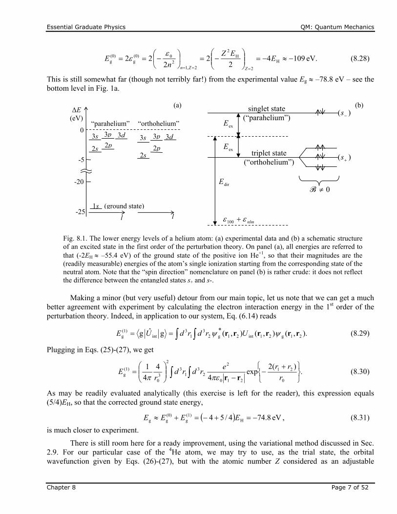
This is still somewhat far (though not terribly far!) from the experimental value Eg –78.8 eV – see the bottom level in Fig. 1a.
Making a minor (but very useful) detour from our main topic, let us note that we can get a much better agreement with experiment by calculating the electron interaction energy in the 1st order of the perturbation theory. Indeed, in application to our system, Eq. (6.14) reads
).,(),(),(gˆg 21g21int21g23
13
int(1)g
* rrrrrr UrdrdUE (8.29)
Plugging in Eqs. (25)-(27), we get
.)(2
exp4
4
4
1
0
21
210
2
23
13
2
30
(1)g
r
rrerdrd
rE
rr (8.30)
As may be readily evaluated analytically (this exercise is left for the reader), this expression equals (5/4)EH, so that the corrected ground state energy,
eV 8.744/54 H(1)g
(0)gg EEEE , (8.31)
is much closer to experiment.
There is still room here for a ready improvement, using the variational method discussed in Sec. 2.9. For our particular case of the 4He atom, we may try to use, as the trial state, the orbital wavefunction given by Eqs. (26)-(27), but with the atomic number Z considered as an adjustable
(a) (b)
Fig. 8.1. The lower energy levels of a helium atom: (a) experimental data and (b) a schematic structure of an excited state in the first order of the perturbation theory. On panel (a), all energies are referred to that (-2EH –55.4 eV) of the ground state of the positive ion He+1, so that their magnitudes are the (readily measurable) energies of the atom’s single ionization starting from the corresponding state of the neutral atom. Note that the “spin direction” nomenclature on panel (b) is rather crude: it does not reflect the difference between the entangled states s+ and s-.
nlm 100
dirE
exE
exE
singlet state (“parahelium”)
triplet state (“orthohelium”)
0B
-25 1s (ground state)
2s
3s
2s
0
2p
3p
ΔE (eV)
-5
-20
3s 3p
2p
3d 3d
l l
“parahelium” “orthohelium”
)( s
)( s
Essential Graduate Physics QM: Quantum Mechanics
Chapter 8 Page 8 of 52
parameter Zef < Z = 2 rather than a fixed number. The physics behind this approach is that the electric charge density (r) = –e(r)2 of each electron forms a negatively charged “cloud” that reduces the effective charge of the nucleus, as seen by the other electron, to Zefe, with some Zef < 2. As a result, the single-particle wavefunction spreads further in space (with the scale r0 = rB/Zef > rB/Z), while keeping its functional form (27) nearly intact. Since the kinetic energy T in the system’s Hamiltonian (25) is proportional to r0
-2 Zef2, while the potential energy is proportional to r0
-1 Zef1, we can write
2g
ef
2g
2
efefg 22
)(
ZZU
ZT
ZZE . (8.32)
Now we can use the fact that according to Eq. (3.212), for any stationary state of a hydrogen-like atom (just as for the classical circular motion in the Coulomb potential), U = 2E, and hence T = E – U = –E. Using Eq. (30), and adding the correction (31) to the potential energy, we get
.24
58
24)( H
ef
2
efefg E
ZZZE
(8.33)
This expression allows an elementary calculation of the optimal value of Zef, and the corresponding minimum of the function Eg(Zef):
eV 5.7785.2,6875.132
512)( Hmingoptef
EEZ . (8.34)
Given the trial state’s crudeness, this number is in surprisingly good agreement with the experimental value cited above, with a difference of the order of 1%.
Now let us return to the main topic of this section – the effects of particle (in this case, electron) indistinguishability. As we have just seen, the ground-level energy of the helium atom is not affected directly by this fact, but the situation is different for its excited states – even the lowest ones. The reasonably good precision of the perturbation theory, which we have seen for the ground state, tells us that we can base our analysis of wavefunctions (e) of the lowest excited state orbitals, on products like 100(rk)nlm(rk’), with n > 1. To satisfy the fermion permutation rule, Pj = –1, we have to take the orbital factor of the state in either the symmetric or the antisymmetric form:
)()()()(2
1),( 21001211002e rrrrrr1 nlmnlm , (8.35)
with the proper total permutation asymmetry provided by the corresponding spin factor (18) or (21), so that the upper/lower sign in Eq. (35) corresponds to the singlet/triplet spin state. Let us calculate the expectation values of the total energy of the system in the first order of the perturbation theory. Plugging Eq. (35) into the 0th-order expression
21e2121e23
13)0(
e ,ˆˆ,* rrrr hhrdrdE , (8.36)
we get two groups of similar terms that differ only by the particle index. We can merge the terms of each pair by changing the notation as (r1 r, r2 r’ ) in one of them, and (r1 r’, r2 r) in the counterpart term. Using Eq. (25), and the mutual orthogonality of the wavefunctions 100(r) and nlm(r), we get the following result:
Orthohelium and parahelium: orbital wavefunctions
Essential Graduate Physics QM: Quantum Mechanics
Chapter 8 Page 9 of 52
.1with ,
)(4
2
2)()(
4
2
2)(
100
3
0
2223
1000
222
100
)0(
e**
n
r'd'r'
e
m'rd
r
e
mE
nlm
nlm'
nlm
rrrr rr
(8.37)
It may be interpreted as the sum of eigenenergies of two separate single particles, one in the ground state 100, and another in the excited state nlm – although actually the electron states are entangled. Thus, in the 0th order of the perturbation theory, the electron entanglement does not affect their energy.
However, the potential energy of the system also includes the interaction term Uint, which does not allow such separation. Indeed, in the 1st approximation of the perturbation theory, the total energy Ee of the system may be expressed as 100 + nlm + Eint
(1), with
),(),(),( 21e21int21e23
13
int)1(
int* rrrrrr UrdrdUE , (8.38)
Plugging Eq. (35) into this result, using the symmetry of the function Uint with respect to the particle number permutation, and the same particle coordinate re-numbering as above, we get
,exdir)1(
int EEE (8.39)
with the following, deceivingly similar expressions for the two components of this sum/difference:
,)()(),()()( 100int10033
dir** ''U'r'drdE nlmnlm rrrrrr (8.40)
.)()(),()()( 100int10033
ex** ''U'r'drdE nlmnlm rrrrrr (8.41)
Since the single-particle orbitals can be always made real, both components are positive – or at least non-negative. However, their physics and magnitude are different. The integral (40), called the direct interaction energy, allows a simple semi-classical interpretation as the Coulomb energy of interacting electrons, each distributed in space with the electric charge density (r) = –e*(r)(r):12
,)()()()(4
)()( 3
100
3100
0
10033dir rdrd
'
'r'drdE nlmnlm
nlm rrrrrr
rr
(8.42)
where (r) are the electrostatic potentials created by the electron “charge clouds”:13
'
'r'd
'
'r'd nlm
nlm rr
rr
rr
rr
)(
4
1)(,
)(
4
1)( 3
0
1003
0100
. (8.43)
However, the integral (41), called the exchange interaction energy, evades a classical interpretation, and (as it is clear from its derivation) is the direct corollary of electrons’ indistinguishability. The magnitude of Eex is also very much different from Edir because the function under the integral (41) disappears in the regions where the single-particle wavefunctions 100(r) and nlm(r) do not overlap. This is in full agreement with the discussion in Sec. 1: if two particles are identical but well separated, i.e. their wavefunctions do not overlap, the exchange interaction disappears,
12 See, e.g., EM Sec. 1.3, in particular Eq. (1.54). 13 Note that the result for Edir correctly reflects the basic fact that a charged particle does not interact with itself, even if its wavefunction is quantum-mechanically spread over a finite space volume. Unfortunately, this is not true for some popular approximate theories of multiparticle systems – see Sec. 4 below.
Exchange interaction
energy
Direct interaction
energy
Essential Graduate Physics QM: Quantum Mechanics
Chapter 8 Page 10 of 52
i.e. measurable effects of particle indistinguishability vanish. (In contrast, the integral (40) decreases with the growing electron separation only slowly, due to the long-range Coulomb interaction.)
Figure 1b shows the structure of an excited energy level, with certain quantum numbers n > 1, l, and m, given by Eqs. (39)-(41). The upper, so-called parahelium14 level, with the energy
,100exdir100para nlmnlm EEE (8.44)
corresponds to the symmetric orbital state and hence to the singlet spin state (18), while the lower, orthohelium level, with ,paraexdir100orth EEEE nlm (8.45)
corresponds to the degenerate triplet spin state (21).
This degeneracy may be lifted by an external magnetic field, whose effect on the electron spins15 is described by the following evident generalization of the Pauli Hamiltonian (4.163),
B
ee21field 2with ˆˆˆˆ
m
eH ,BBB Sss , (8.46)
where
21 ˆˆˆ ssS , (8.47)
is the operator of the (vector) sum of the system of two spins.16 To analyze this effect, we need first to make one more detour, to address the general issue of spin addition. The main rule17 here is that in a full analogy with the net spin of a single particle, defined by Eq. (5.170), the net spin operator (47) of any
system of two spins, and its component zS along the (arbitrarily selected) z-axis, obey the same commutation relations (5.168) as the component operators, and hence have the properties similar to those expressed by Eqs. (5.169) and (5.175):
SMSMSMMSSMSSSMSS SSSSzSS with ,,,ˆ,,1,ˆ 22 , (8.48)
where the ket vectors correspond to the coupled basis of joint eigenstates of the operators of S2 and Sz (but not necessarily all component operators – see again the Venn shown in Fig. 5.12 and its discussion, with the replacements S, L s1,2 and J S). Repeating the discussion of Sec. 5.7 with these replacements, we see that in both coupled and uncoupled bases, the net magnetic number MS is simply expressed via those of the components
14 This terminology reflects the historic fact that the observation of two different hydrogen-like spectra, corresponding to the opposite signs in Eq. (39), was first taken as evidence for two different species of 4He, which were called, respectively, the “orthohelium” and the “parahelium”. 15 As we know from Sec. 6.4, the field also affects the orbital motion of the electrons, so that the simple analysis based on Eq. (46) is strictly valid only for the s excited state (l = 0, and hence m = 0). However, the orbital effects of a weak magnetic field do not affect the triplet level splitting we are analyzing now. 16 Note that similarly to Eqs. (22) and (25), here the uppercase notation of the component spins is replaced with their lowercase notation, to avoid any possibility of their confusion with the total spin of the system. 17 Since we already know that the spin of a particle is physically nothing more than a (specific) part of its angular momentum, the similarity of the properties (48) of the sum (47) of spins of different particles to those of the sum (5.170) of different spin components of the same particle it very natural, but still has to be considered as a new fact – confirmed by a vast body of experimental data.
Essential Graduate Physics QM: Quantum Mechanics
Chapter 8 Page 11 of 52
21 ssS mmM . (8.49)
However, the net spin quantum number S (in contrast to the Nature-given spins s1,2 of its elementary components) is not universally definite, and we may immediately say only that it has to obey the following analog of the relation l – s j (l + s) discussed in Sec. 5.7:
2121 ssSss . (8.50)
What exactly S is (within these limits), depends on the spin state of the system.
For the simplest case of two spin-½ components, each with s = ½ and ms = ½, Eq. (49) gives three possible values of MS, equal to 0 and 1, while Eq. (50) limits the possible values of S to just either 0 or 1. Using the last of Eqs. (48), we see that the possible combinations of the quantum numbers are
.1,0
,1 and
,0
,0
SS M
S
M
S (8.51)
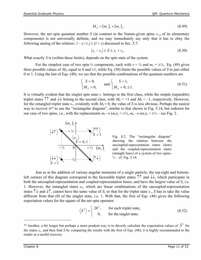
It is virtually evident that the singlet spin state s– belongs to the first class, while the simple (separable) triplet states and belong to the second class, with MS = +1 and MS = –1, respectively. However, for the entangled triplet state s+, evidently with MS = 0, the value of S is less obvious. Perhaps the easiest way to recover it18 to use the “rectangular diagram”, similar to that shown in Fig. 5.14, but redrawn for our case of two spins, i.e., with the replacements ml (ms)1 = ½, ms (ms)2 = ½ – see Fig. 2.
Just as at the addition of various angular momenta of a single particle, the top-right and bottom-left corners of this diagram correspond to the factorable triplet states and , which participate in both the uncoupled-representation and coupled-representation bases, and have the largest value of S, i.e. 1. However, the entangled states s, which are linear combinations of the uncoupled-representation states and , cannot have the same value of S, so that for the triplet state s+, S has to take the value different from that (0) of the singlet state, i.e. 1. With that, the first of Eqs. (48) gives the following expectation values for the square of the net spin operator:
state.singlet for the0,
state,et each triplfor ,2
22
S (8.52)
18 Another, a bit longer but perhaps a more prudent way is to directly calculate the expectation values of 2S for the states s, and then find S by comparing the results with the first of Eqs. (48); it is highly recommended to the reader as a useful exercise.
Fig. 8.2. The “rectangular diagram” showing the relation between the uncoupled-representation states (dots) and the coupled-representation states (straight lines) of a system of two spins-½ – cf. Fig. 5.14.
2sm
½½ 0 1sm
½
½
1S
1S
1,0Ss
Essential Graduate Physics QM: Quantum Mechanics
Chapter 8 Page 12 of 52
Note that for the entangled triplet state s+, whose ket-vector (20) is a linear superposition of two kets of states with opposite spins, this result is highly counter-intuitive, and shows how careful we should be interpreting entangled quantum states. (As will be discussed in Chapter 10, the entanglement brings even more surprises for quantum measurements.)
Now we may return to the particular issue of the magnetic field effect on the triplet state of the 4He atom. Directing the z-axis along the field, we may reduce Eq. (46) to
zz
SSH
ˆ2 Befield
ˆˆ BB . (8.53)
Since all three triplet states (21) are eigenstates, in particular, of the operator zS , and hence of the Hamiltonian (53), we may use the second of Eqs. (48) to calculate their energy change simply as
. state triplet factorable for the,1
, state triplet entangled for the,0
, state triplet factorable for the,1
2 BBfield 2 sME S BB (8.54)
This splitting of the “orthohelium” level is schematically shown in Fig. 1b.19
8.3. Multiparticle systems
Leaving several other problems on two-particle systems for the reader’s exercise, let me proceed to the discussion of systems with N > 2 indistinguishable particles, whose list notably includes atoms, molecules, and condensed-matter systems. In this case, Eq. (7) for fermions is generalized as
Nk'kkk ,...,2,1, allfor ,ˆ' P , (8.55)
where the operator 'ˆ
kkP permutes particles with numbers k and k’. As a result, for systems with non-
directly-interacting fermions, the Pauli principle forbids any state in which any two particles have similar single-particle wavefunctions. Nevertheless, it permits two fermions to have similar orbital wavefunctions, provided that their spins are in the singlet state (18), because this satisfies the permutation requirement (55). This fact is of paramount importance for the ground state of the systems whose Hamiltonians do not depend on spin because it allows the fermions to be in their orbital single-particle ground states, with two electrons of the spin singlet sharing the same orbital state. Hence, for the limited (but very important!) goal of finding ground-state energies of multi-fermion systems with negligible direct interaction, we may ignore the actual singlet spin structure, and reduce the Pauli
19 It is interesting that another very important two-electron system, the hydrogen (H2) molecule, which was briefly discussed in Sec. 2.6, also has two similarly named forms, parahydrogen and orthohydrogen. However, their difference is due to two possible (respectively, singlet and triplet) states of the system of two spins of the two hydrogen nuclei – protons, which are also spin-½ particles. The resulting energy of the parahydrogen is lower than that of the orthohydrogen by only ~45 meV per molecule – the difference comparable with kBT at room temperature (~26 meV). As a result, at the ambient conditions, the equilibrium ratio of these two spin isomers is close to 3:1. Curiously, the theoretical prediction of this minor effect by W. Heisenberg (together with F. Hund) in 1927 was cited in his 1932 Nobel Prize award as the most noteworthy application of quantum theory.
Essential Graduate Physics QM: Quantum Mechanics
Chapter 8 Page 13 of 52
exclusion principle to the simple picture of single-particle orbital energy levels, each “occupied with two fermions”.
As a very simple example, let us find the ground energy of five fermions, confined in a hard-wall, cubic-shaped 3D volume of side a, ignoring their direct interaction. From Sec. 1.7, we know the single-particle energy spectrum of the system:
,...2,1,, and,2
with ,2
22
0222
0,, zyxzyxnnn nnnma
nnnzyx
(8.56)
so that the lowest-energy states are:
- one ground state with {nx,ny,nz} = {1,1,1}, and energy 111= (12+12+12)0 = 30, and
- three excited states, with {nx,ny,nz} equal to either {2,1,1}, or {1,2,1}, or {1,1,2}, with equal energies 211= 121 = 112 = (22+12+12)0 = 60.
According to the above simple formulation of the Pauli principle, each of these orbital energy levels can accommodate up to two fermions. Hence the lowest-energy (ground) state of the five-fermion system is achieved by placing two of them on the ground level 111 = 30, and the remaining three particles, in any of the degenerate “excited” states of energy 60, so that the ground-state energy of the system is
.12
2463322
22
000g maE
(8.57)
Moreover, in many cases, relatively weak interaction between fermions does not blow up such a simple quantum state classification scheme qualitatively, and the Pauli principle allows tracing the order of single-particle state filling. This is exactly the simple approach that has been used in our discussion of atoms in Sec. 3.7. Unfortunately, it does not allow for a more specific characterization of the ground states of most atoms, in particular the evaluation of the corresponding values of the quantum numbers S, L, and J that characterize the net angular momenta of the atom, and hence its response to an external magnetic field. These numbers are defined by relations similar to Eqs. (48), each for the corresponding vector operator of the net angular momenta:
N
kk
N
kk
N
kk
111
ˆˆ,ˆˆ,ˆˆ jJlLsS ; (8.58)
note that these definitions are consistent with Eq. (5.170) applied both to the angular momenta sk, lk, and jk of each particle, and to the full vectors S, L, and J. When the numbers S, L, and J for a state are known, they are traditionally recorded in the form of the so-called Russell-Saunders symbols:20
,12J
S L (8.59)
where S and J are the corresponding values of these quantum numbers, while L is a capital letter, encoding the quantum number L – via the same spectroscopic notation as for single particles (see Sec. 3.6): L = S for L = 0, L = P for L = 1, L = D for L = 2, etc. (The reason why the front superscript of the Russel-Saunders symbol lists 2S + 1 rather than just S, is that according to the last of Eqs. (48), it
20 Named after H. Russell and F. Saunders, whose pioneering (circa 1925) processing of experimental spectral-line data has established the very idea of vector addition of the electron spins, described by the first of Eqs. (58).
Essential Graduate Physics QM: Quantum Mechanics
Chapter 8 Page 14 of 52
shows the number of possible values of the quantum number MS, which characterizes the state’s spin degeneracy, and is called its multiplicity.)
For example, for the simplest, hydrogen atom (Z = 1), with its single electron in the ground 1s state, L = l = 0, S = s = ½, and J = S = ½, so that its Russell-Saunders symbol is 2S1/2. Next, the discussion of the helium atom (Z = 2) in the previous section has shown that in its ground state L = 0 (because of the 1s orbital state of both electrons), and S = 0 (because of the singlet spin state), so that the total angular momentum also vanishes: J = 0. As a result, the Russell-Saunders symbol is 1S0. The structure of the next atom, lithium (Z = 3) is also easy to predict, because, as was discussed in Sec. 3.7, its ground-state electron configuration is 1s22s1, i.e. includes two electrons in the “helium shell”, i.e. on the 1s orbitals (now we know that they are actually in a singlet spin state), and one electron in the 2s state, of higher energy, also with zero orbital momentum, l = 0. As a result, the total L in this state is evidently equal to 0, and S is equal to ½, so that J = ½, meaning that the Russell-Saunders symbol of lithium is 2P1/2. Even in the next atom, beryllium (Z = 4), with the ground state configuration 1s22s2, the symbol is readily predictable, because none of its electrons has non-zero orbital momentum, giving L = 0. Also, each electron pair is in the singlet spin state, i.e. we have S = 0, so that J = 0 – the quantum number set described by the Russell-Saunders symbol 1S0 – just as for helium.
However, for the next, boron atom (Z = 5), with its ground-state electron configuration 1s22s22p1 (see, e.g., Fig. 3.24), there is no obvious way to predict the result. Indeed, this atom has two pairs of electrons, with opposite spins, on its two lowest s-orbitals, giving zero contributions to the net S, L, and J. Hence these total quantum numbers may be only contributed by the last, fifth electron with s = ½ and l = 1, giving S = ½, L = 1. As was discussed in Sec. 5.7 for the single-particle case, the vector addition of the angular momenta S and L enables two values of the quantum number J: either L + S = ³/2 or L – S = ½. Experiment shows that the difference between the energies of these two states is very small (~2 meV), so that at room temperature (with kBT 26 meV) they are both occupied, with the genuine ground state having J = ½, so that its Russell-Saunders symbol is 2P1/2.
Such energy differences, which become larger for heavier atoms, are determined both by the Coulomb and spin-orbit21 interactions between the electrons. Their quantitative analysis is rather involved (see below), but the results tend to follow simple phenomenological Hund rules, with the following hierarchy:
Rule 1. For a given electron configuration, the ground state has the largest possible S, and hence the largest multiplicity 2S + 1.
Rule 2. For a given S, the ground state has the largest possible L.
Rule 3. For given S and L, J has its smallest possible value, L – S , if the given sub-shell {n, l} is filled not more than by half, while in the opposite case, J has its largest possible value, L + S.
Let us see how these rules work for the boron atom we have just discussed. For it, the Hund Rules 1 and 2 are satisfied automatically, while the sub-shell {n = 2, l = 1}, which can house up to 2(2l + 1) = 6 electrons, is filled with just one 2p electron, i.e. by less than a half of the maximum value. As a result, the Hund Rule 3 predicts the ground state’s value J = ½, in agreement with experiment.
21 In light atoms, the spin-orbit interaction is so weak that it may be reasonably well described as an interaction of the total momenta L and S of the system – the so-called LS (or “Russell-Saunders”) coupling. On the other hand, in very heavy atoms, the interaction is effectively between the net momenta jk = lk + sk of the individual electrons – the so-called jj coupling. This is the reason why in such atoms the Hund rule 3 may be violated.
Essential Graduate Physics QM: Quantum Mechanics
Chapter 8 Page 15 of 52
Generally, for lighter atoms, the Hund rules are well obeyed. However, the lower down the Hund rule hierarchy, the less “powerful” the rules are, i.e. the more often they are violated in heavier atoms.
Now let us discuss possible approaches to a quantitative theory of multiparticle systems – not only atoms. As was discussed in Sec. 1, if fermions do not interact directly, the stationary states of the system have to be the antisymmetric eigenstates of the permutation operator, i.e. satisfy Eq. (55). To understand how such states may be formed from the single-electron ones, let us return for a minute to the case of two electrons, and rewrite Eq. (11) in the following compact form:
2,number particle
1,number particle
2
1
2
1
2 state 1 state
'β
'β''
(8.60a)
where the direct product signs are just implied. In this way, the Pauli principle is mapped on the well-known property of matrix determinants: if any of two columns of a matrix coincide, its determinant vanishes. This Slater determinant approach22 may be readily generalized to N fermions occupying any N (not necessarily the lowest-energy) single-particle states , ’, ’’, etc:
list
particle
!
1
list state
2/1N
N
"'β
"'β
"'β
N
(8.60b)
The Slater determinant form is extremely nice and compact – in comparison with direct writing of a sum of N! products, each of N ket factors. However, there are two major problems with using it for practical calculations:
(i) For the calculation of any bra-ket product (say, within the perturbation theory) we still need to spell out each bra- and ket-vector as a sum of component terms. Even for a limited number of electrons (say N ~ 102 in a typical atom), the number N! ~ 10160 of terms in such a sum is impracticably large for any analytical or numerical calculation.
(ii) In the case of interacting fermions, the Slater determinant does not describe the eigenvectors of the system; rather the stationary state is a superposition of such basis functions, i.e. of the Slater determinants – each for a specific selection of N states from the full set of single-particle states – that is generally larger than N.
For atoms and simple molecules, whose filled-shell electrons may be excluded from an explicit analysis (by describing their effects, approximately, with effective pseudo-potentials), the effective number N may be reduced to a smaller number Nef of the order of 10, so that Nef! < 106, and the Slater determinants may be used for numerical calculations – for example, in the Hartree-Fock theory – see the next section. However, for condensed-matter systems, such as metals and semiconductors, with the
22 It was suggested in 1929 by John C. Slater.
Slater determinant
Essential Graduate Physics QM: Quantum Mechanics
Chapter 8 Page 16 of 52
number of free electrons is of the order of 1023 per cm3, this approach is generally unacceptable, though with some smart tricks (such as using the crystal’s periodicity) it may be still used for some approximate (also mostly numerical) calculations.
These challenges make the development of a more general theory that would not use particle numbers (which are superficial for indistinguishable particles to start with) a must for getting any final analytical results for multiparticle systems. The most effective formalism for this purpose, which avoids particle numbering at all, is called the second quantization.23 Actually, we have already discussed a particular version of this formalism, for the case of the 1D harmonic oscillator, in Sec. 5.4. As a reminder, after the definition (5.65) of the “creation” and “annihilation” operators via those of the particle’s coordinate and momentum, we have derived their key properties (5.89),
11ˆ,1ˆ 2/12/1 † nnnannna , (8.61)
where n are the stationary (Fock) states of the oscillator. This property allows an interpretation of the operators’ actions as the creation/annihilation of a single excitation with the energy 0 – thus justifying the operator names. In the next chapter, we will show that such excitation of an electromagnetic field mode may be interpreted as a massless boson with s = 1, called the photon.
In order to generalize this approach to arbitrary bosons, not appealing to a specific system, we may use relations similar to Eq. (61) to define the creation and annihilation operators. The definitions look simple in the language of the so-called Dirac states, described by ket-vectors
,...,..., 21 jNNN , (8.62)
where Nj is the state occupancy, i.e. the number of bosons in the single-particle state j. Let me emphasize that here the indices 1, 2, …j,… number single-particle states (including their spin parts) rather than particles. Thus the very notion of an individual particle’s number is completely (and for indistinguishable particles, very relevantly) absent from this formalism. Generally, the set of single-particle states participating in the Dirac state may be selected arbitrarily, provided that it is full and orthonormal in the sense
......2211
2121 ,,,,jj
j'j'
''
N'NN'NN'N...N...,NN...N...,NN , (8.63)
though for systems of non- (or weakly) interacting bosons, using the stationary states of individual particles in the system under analysis is almost always the best choice.
Now we can define the particle annihilation operator as follows:
.,...1,...,,...,...,ˆ 212/1
21 jjjj NNNNNNNa (8.64)
Note that the pre-ket coefficient, similar to that in the first of Eqs. (61), guarantees that any attempt to annihilate a particle in an initially unpopulated state gives the non-existing (“null”) state:
0,...0,...,ˆ 21 jj NNa , (8.65)
23 It was invented (first for photons and then for arbitrary bosons) by P. Dirac in 1927, and then modified in 1928 for fermions by E. Wigner and P. Jordan. Note that the term “second quantization” is rather misleading for the non-relativistic applications we are discussing here, but finds certain justification in the quantum field theory.
Dirac state
Boson annihilation operator
Essential Graduate Physics QM: Quantum Mechanics
Chapter 8 Page 17 of 52
where the symbol 0j means zero occupancy of the jth state. According to Eq. (63), an equivalent way to write Eq. (64) is
...,...,..,,.ˆ,...,...,, 1...,2211
2/12121
jjjjj
'j
''
NN'N'NN'NNNNNaNNN (8.66)
According to the general Eq. (4.65), the matrix element of the Hermitian conjugate operator †ˆ ja is
,...1
...,...1,...,,...,...,,
,...,...,ˆ,...,...,,,...,...,ˆ,...,...,
,2211
2/1
,2211
2/1
21
2/1
21
21212121
1...
1...
*†
jjj
jj
'j
'j
'''jj
'j
''jjjj
'j
''
N'NN'NN'N
N'NN'NN'N
N
NN,NNNNNN
N,NNaNNNNNNaN,NN
(8.67)
meaning that
,,...1,...,,1,...,...,,ˆ 212/1
21† jjjj NNNNNNNa (8.68)
in total compliance with the second of Eqs. (61). In particular, this particle creation operator allows the description of the generation of a single particle from the vacuum (not null!) state 0, 0, …:
,0,...1,...,0,00,...,0,...,0,0ˆ†jjja (8.69)
and hence a product of such operators may create, from the vacuum, a multiparticle state with an arbitrary set of occupancies: 24
.,...,!...!,...0,0 ...ˆ...ˆˆˆ...ˆˆ 212/1
21
222
111
times
†††
times
†††
21
NNNNaaaaaa
NN
(8.70)
Next, combining Eqs. (64) and (68), we get
,,...,...,,,...,...,ˆˆ 2121†
jjjjj NNNNNNNaa (8.71)
so that, just as for the particular case of harmonic oscillator excitations, the operator
jjj aaN ˆˆˆ † (8.72)
“counts” the number of particles in the jth single-particle state, while preserving the whole multiparticle state. Acting on a state by the creation-annihilation operators in the reverse order, we get
.,...,...,,1,...,...,,ˆˆ 2121†
jjjjj NNNNNNNaa (8.73)
Eqs. (71) and (73) show that for any state of a multiparticle system (which may be represented as a linear superposition of Dirac states with all possible sets of numbers Nj), we may write
,ˆˆ,ˆˆˆˆˆ ††† Iaaaaaa jjjjjj
(8.74)
24 The resulting Dirac state is not an eigenstate of every multiparticle Hamiltonian. However, we will see below that for a set of non-interacting particles it is a stationary state, so that the full set of such states may be used as a good basis in perturbation theories of systems of weakly interacting particles.
Boson creation operator
Number- counting operator
Essential Graduate Physics QM: Quantum Mechanics
Chapter 8 Page 18 of 52
again in agreement with what we had for the 1D oscillator – cf. Eq. (5.68). According to Eqs. (63), (64), and (68), the creation and annihilation operators corresponding to different single-particle states do commute, so that Eq. (74) may be generalized as
''ˆˆ,ˆ †
jjjj Iaa
, (8.75)
while the similar operators commute, regardless of which states do they act upon:
0ˆ,ˆˆ,ˆ ††
j'jj'j aaaa . (8.76)
As was mentioned earlier, a major challenge in the Dirac approach is to rewrite the Hamiltonian of a multiparticle system, that naturally carries particle numbers k (see, e.g., Eq. (22) for k = 1, 2), in the second quantization language, in which there are no these numbers. Let us start with single-particle components of such Hamiltonians, i.e. operators of the type
N
kkfF
1
ˆˆ . (8.77)
where all N operators kf are similar, besides that each of them acts on one specific (kth) particle, and N
is the total number of particles in the system, which is evidently equal to the sum of single-particle state occupancies: .
jjNN (8.78)
The most important examples of such operators are the kinetic energy of N similar single particles, and their potential energy in an external field:
N
k
k
m
pT
1
2
2
ˆˆ , .)(ˆˆ1
N
kkuU r (8.79)
For bosons, instead of the Slater determinant (60), we have to write a similar expression, but without the sign alternation at permutations:
P N
jj "'
N
NNNN
operands
2/1
11 ......
!
!...!...,...,... , (8.80)
sometimes called the permanent. Note again that the left-hand side of this relation is written in the Dirac notation (that does not use particle numbering), while on its right-hand side, just in relations of Secs. 1 and 2, the particle numbers are coded with the positions of the single-particle states inside the state vectors, and the summation is over all different permutations of the states in the ket – cf. Eq. (10). (According to the basic combinatorics,25 there are N!/(N1!...Nj!...) such permutations, so that the front coefficient in Eq. (80) ensures the normalization of the Dirac state, provided that the single-particle states , ’, …are normalized.) Let us use Eq. (80) to spell out the following matrix element for a system with (N –1) particles:
25 See, e.g., MA Eq. (2.3).
Bosonic operators: commutation relations
Single- particle operator
Essential Graduate Physics QM: Quantum Mechanics
Chapter 8 Page 19 of 52
,......ˆ......)!1(
)!...1)!...(1!...(
,...,...1...ˆ,...1,......
1 1
1
1
2/1'
'1
NP NP
N
kkjj
jj
j'jj'j
"'f"'NNN
NNN
NNFNN
(8.81)
where all non-specified occupation numbers in the corresponding positions of the bra- and ket-vectors
are equal to each other. Each single-particle operator kf participating in the operator sum, acts on the
bra- and ket-vectors of states only in one (kth) position, giving the following result, independent of the position number:
jj'j'jj'kj fffkk
ˆˆposition in position n ththi
. (8.82)
Since in both permutation sets participating in Eq. (81), with (N – 1) state vectors each, all positions are equivalent, we can fix the position (say, take the first one) and replace the sum over k with the multiplication by of the bracket by (N – 1). The fraction of permutations with the necessary bra-vector (with number j) in that position is Nj/(N – 1), while that with the necessary ket-vector (with number j’) in the same position is Nj’/(N – 1). As the result, the permutation sum in Eq. (81) reduces to
,............11
)1(2 2
''
NP NPjj
jj "'"'fN
N
N
NN (8.83)
where our specific position k is now excluded from both the bra- and ket-vector permutations. Each of these permutations now includes only (Nj – 1) states j and (Nj’ – 1) states j’, so that, using the state orthonormality, we finally arrive at a very simple result:
.
)!...1)!...(1!...(
)!2(
11)1(
)!1(
)!...1)!...(1!...(
,...,...1...ˆ,...1,......
2/1
'1'
'2/11
jj'j'j
jjjj
jjj'j
j'j
j'jj'j
fNN
NNN
Nf
N
N
N
NNNN
N
NNN
NNFNN
(8.84)
On the other hand, let us calculate matrix elements of the following operator:
',
ˆ†ˆjj
j'jjj' aaf . (8.85)
A direct application of Eqs. (64) and (68) shows that the only non-vanishing of the elements are
'2/1
''''' ,...,...,1...ˆ†ˆ,...1,...... jjjjjjjjjjjj fNNNNaafNN . (8.86)
But this is exactly the last form of Eq. (84), so that in the basis of Dirac states, the operator (77) may be represented as
j'j
j'jjj' aafF,
ˆˆˆ † . (8.87)
This beautifully simple relation is the key formula of the second quantization theory, and is essentially the Dirac-language analog of Eq. (4.59) of the single-particle quantum mechanics. Each term of the sum (87) may be described by a very simple mnemonic rule: for each pair of single-particle states
Single- particle
operator in Dirac
language
Essential Graduate Physics QM: Quantum Mechanics
Chapter 8 Page 20 of 52
j and j’, annihilate a particle in the state j’, create one in the state j, and weigh the result with the corresponding single-particle matrix element. One of the corollaries of Eq. (87) is that the expectation value of an operator whose eigenstates coincide with the Dirac states is
,,......ˆ,...... j
jjjjj NfNFNF (8.88)
with an evident physical interpretation as the sum of single-particle expectation values over all states, weighed by the occupancy of each state.
Proceeding to fermions, which have to obey the Pauli principle, we immediately notice that any occupation number Nj may only take two values, 0 or 1. To account for that, and also make the key relation (87) valid for fermions as well, the creation-annihilation operators are defined by the following relations:
,,...0,...,,)1(,...1,...,,ˆ,0,...0,...,,ˆ 212121)1,1(
jjjjj NNNNaNNa j (8.89)
,0,...1,...,,ˆ,,...1,...,,)1(,...0,...,,ˆ 212121†)1,1(†
jjjjj NNaNNNNa j (8.90)
where the symbol (J, J’) means the sum of all occupancy numbers in the states with numbers from J to J’, including the border points:
,),(
J'
JjjNJ'J (8.91)
so that the sum participating in Eqs. (89)-(90) is the total occupancy of all states with the numbers below j. (The states are supposed to be numbered in a fixed albeit arbitrary order.) As a result, these relations may be conveniently summarized in the following verbal form: if an operator replaces the jth state’s occupancy with the opposite one (either 1 with 0, or vice versa), it also changes the sign before the result if (and only if) the total number of particles in the states with j’ < j is odd.
Let us use this (perhaps somewhat counter-intuitive) sign alternation rule to spell out the ket-vector 11 of a completely filled two-state system, formed from the vacuum state 00 in two different ways. If we start by creating a fermion in the state 1, we get
1,11,1)1(0,1ˆ0,0ˆˆ,0,10,1)1(0,0ˆ 1212
01
†††† aaaa , (8.92a)
while if the operator order is different, the result is
,1,11,1)1(1,0ˆ0,0ˆˆ,1,01,0)1(0,0ˆ 0121
02
†††† aaaa (8.92b)
so that
00,0ˆˆˆˆ ††††1221
aaaa . (8.93)
Since the action of any of these operator products on any initial state rather than the vacuum one also gives the null ket, we may write the following operator equality:
.0ˆ,ˆˆˆˆˆ ††††††211221
aaaaaa (8.94)
It is straightforward to check that this result is valid for Dirac vectors of an arbitrary length, and does not depend on the occupancy of other states, so that we may generalize it as
Fermion creation-annihilation operators
Essential Graduate Physics QM: Quantum Mechanics
Chapter 8 Page 21 of 52
0ˆ,ˆˆ,ˆ ††
j'jj'j aaaa ; (8.95)
these equalities hold for j = j’ as well. On the other hand, an absolutely similar calculation shows that the mixed creation-annihilation commutators do depend on whether the states are different or not:26
jj'j'j Iaa ˆ,ˆ †
. (8.96)
These equations look very much like Eqs. (75)-(76) for bosons, “only” with the replacement of commutators with anticommutators. Since the core laws of quantum mechanics, including the operator compatibility (Sec. 4.5) and the Heisenberg equation (4.199) of operator evolution in time, involve commutators rather than anticommutators, one might think that all the behavior of bosonic and fermionic multiparticle systems should be dramatically different. However, the difference is not as big as one could expect; indeed, a straightforward check shows that the sign factors in Eqs. (89)-(90) just compensate those in the Slater determinant, and thus make the key relation (87) valid for the fermions as well. (Indeed, this is the very goal of the introduction of these factors.)
To illustrate this fact on the simplest example, let us examine what does the second quantization formalism say about the dynamics of non-interacting particles in the system whose single-particle properties we have discussed repeatedly, namely two nearly-similar potential wells, coupled by tunneling through the separating potential barrier – see, e.g., Figs. 2.21 or 7.4. If the coupling is so small that the states localized in the wells are only weakly perturbed, then in the basis of these states, the single-particle Hamiltonian of the system may be represented by the 22 matrix (5.3). With the energy reference selected at the middle between the energies of unperturbed states, the coefficient b vanishes, this matrix is reduced to
,with ,h yxz
z iccccc
cc
σc (8.97)
and its eigenvalues to
.with ,2/1222
zyx ccccc c (8.98)
Now following the recipe (87), we can use Eq. (97) to represent the Hamiltonian of the whole system of particles in terms of the creation-annihilation operators:
,ˆ†ˆˆ†ˆˆ†ˆˆ†ˆˆ22122111 aacaacaacaacH zz (8.99)
where †2,1a and 2,1a are the operators of creation and annihilation of a particle in the corresponding
potential well. (Again, in the second quantization approach the particles are not numbered at all!) As Eq. (72) shows, the first and the last terms of the right-hand side of Eq. (99) describe the particle energies 1,2 = cz in uncoupled wells,
,ˆˆˆˆ,ˆˆˆˆ 2222211111†† NNcaacNNcaac zzzz (8.100)
26 A by-product of this calculation is proof that the operator defined by Eq. (72) counts the number of particles Nj (now equal to either 1 or 0), just at it does for bosons.
Fermionic operators:
commutation relations
Essential Graduate Physics QM: Quantum Mechanics
Chapter 8 Page 22 of 52
while the sum of the middle two terms is the second-quantization description of tunneling between the wells.
Now we can use the general Eq. (4.199) of the Heisenberg picture to spell out the equations of motion of the creation-annihilation operators. For example,
.ˆ†ˆ,ˆˆ†ˆ,ˆˆ†ˆ,ˆˆ†ˆ,ˆˆ,ˆˆ 22112121111111
aaacaaacaaacaaacHaai zz
(8.101)
Since the Bose and Fermi operators satisfy different commutation relations, one could expect the right-hand side of this equation to be different for bosons and fermions. However, it is not so. Indeed, all commutators on the right-hand side of Eq. (101) have the following form:
.ˆˆˆˆˆˆˆˆ,ˆ †††jj"j'j"j'jj"j'j aaaaaaaaa
(8.102)
As Eqs. (74) and (94) show, the first pair product of operators on the right-hand side may be recast as
,ˆˆˆˆˆ ††jj'jj'j'j aaIaa (8.103)
where the upper sign pertains to bosons and the lower one to fermions, while according to Eqs. (76) and (95), the very last pair product in Eq. (102) is
,ˆˆˆˆ j"jjj" aaaa (8.104)
with the same sign convention. Plugging these expressions into Eq. (102), we see that regardless of the particle type, there is a universal (and generally very useful) commutation relation
jj'j"j"j'j aaaa ˆˆˆ,ˆ †
, (8.105)
valid for both bosons and fermions. As a result, the Heisenberg equation of motion for the operator 1a ,
and the equation for 2a (which may be obtained absolutely similarly), are also universal:27
.ˆˆˆ
,ˆˆˆ
212
211
acacai
acacai
z
z
(8.106)
This is a system of two coupled, linear differential equations, which is similar to the equations for the c-number probability amplitudes of single-particle wavefunctions of a two-level system – see, e.g., Eq. (2.201) and the model solution of Problem 4.25. Their general solution is a linear superposition
.expˆ)(ˆ )(2,12,1
tta (8.107)
As usual, to find the exponents , it is sufficient to plug in a particular solution tta expˆ)(ˆ 2,12,1
into Eq. (106) and require that the determinant of the resulting homogeneous, linear system for the “coefficients” (actually, time-independent operators) 2,1 equals zero. This gives us the following
characteristic equation
27 Equations of motion for the creation operators †ˆ 2,1a are just the Hermitian-conjugates of Eqs. (106), and do not
add any new information about the system’s dynamics.
Essential Graduate Physics QM: Quantum Mechanics
Chapter 8 Page 23 of 52
0
icc
cic
z
z , (8.108)
with two roots = i/2, where 2c/ – cf. Eq. (5.20). Now plugging each of the roots, one by one, into the system of equations for 2,1 , we can find these operators, and hence the general solution of
system (98) for arbitrary initial conditions.
Let us consider the simple case cy = cz = 0 (meaning in particular that the wells are exactly aligned, see Fig. 2.21), so that /2 c = cx; then the solution of Eq. (106) is
.2
cos)0(ˆ2
sin)0(ˆ)(ˆ,2
sin)0(ˆ2
cos)0(ˆ)(ˆ 212211
ta
taita
tai
tata
(8.109)
Multiplying the first of these relations by its Hermitian conjugate, and ensemble-averaging the result, we get
.
2cos
2sin)0(ˆ)0(ˆ)0(ˆ)0(ˆ
2sin)0(ˆ)0(ˆ
2cos)0(ˆ)0(ˆ)(ˆ)(ˆ
1221
222
211111
††
†††
ttaaaai
taa
taatataN
(8.110)
Let the initial state of the system be a single Dirac state, i.e. have a definite number of particles in each well; in this case, only the two first terms on the right-hand side of Eq. (110) are different from zero, giving:28
.2
sin)0(2
cos)0( 22
211
tN
tNN
(8.111)
For one particle, initially placed in either well, this gives us our old result (2.181) describing the usual quantum oscillations of the particle between two wells with the frequency . However, Eq. (111) is valid for any set of initial occupancies; let us use this fact. For example, starting from two particles, with initially one particle in each well, we get N1 = 1, regardless of time. So, the occupancies do not oscillate, and no experiment may detect the quantum oscillations, though their frequency is still formally present in the time evolution equations. This fact may be interpreted as the simultaneous quantum oscillations of two particles between the wells, exactly in anti-phase. For bosons, we can go on to even larger occupancies by preparing the system, for example, in the state with N1(0) = N, N2(0) = 0. The result (111) says that in this case, we see that the quantum oscillation amplitude increases N-fold; this is a particular manifestation of the general fact that bosons can be (and evolve in time) in the same quantum state. On the other hand, for fermions we cannot increase the initial occupancies beyond 1, so that the largest oscillation amplitude we can get is if we initially fill just one well.
The Dirac approach may be readily generalized to more complex systems. For example, Eq. (99) implies that an arbitrary system of potential wells with weak tunneling coupling between the adjacent wells may be described by the Hamiltonian
j j'j
j'jjj'jjj aaaaH ,h.c. ˆˆˆ,
†† (8.112)
28 For the second well’s occupancy, the result is complementary, N2(t) = N1(0)sin2t + N2(0)cos2t , giving in particular a good sanity check: N1(t) + N2(t) = N1(0) + N2(0) = const.
Quantum oscillations:
second quantization
form
Essential Graduate Physics QM: Quantum Mechanics
Chapter 8 Page 24 of 52
where the symbol {j, j’} means that the second sum is restricted to pairs of next-neighbor wells – see, e.g., Eq. (2.203) and its discussion. Note that this Hamiltonian is still a quadratic form of the creation-annihilation operators, so the Heisenberg-picture equations of motion of these operators are still linear, and its exact solutions, though possibly cumbersome, may be studied in detail. Due to this fact, the Hamiltonian (112) is widely used for the study of some phenomena, for example, the very interesting Anderson localization effects, in which a random distribution of the localized-site energies j prevents tunneling particles, within a certain energy range, from spreading to unlimited distances.29
8.4. Perturbative approaches
The situation becomes much more difficult if we need to account for direct interactions between the particles. Let us assume that the interaction may be reduced to that between their pairs (as it is the case at their Coulomb interaction and most other interactions30), so that it may be described by the following “pair-interaction” Hamiltonian
,),(ˆ2
1ˆ
' 1',
intint
N
kkkk
k'kuU rr (8.113)
with the front factor of ½ compensating the double-counting of each particle pair. The translation of this operator to the second-quantization form may be done absolutely similarly to the derivation of Eq. (87), and gives a similar (though naturally more involved) result
,ˆˆˆˆ2
1ˆ,,,
int††
l'lj'jll'j'jjj'll' aaaauU (8.114)
where the two-particle matrix elements are defined similarly to Eq. (82):
.ˆint l'lj'jjj'll' uu (8.115)
The only new feature of Eq. (114) is a specific order of the indices of the creation operators. Note the mnemonic rule of writing this expression, similar to that for Eq. (87): each term corresponds to moving a pair of particles from states l and l’ to states j’ and j (in this order!) factored with the corresponding two-particle matrix element (115).
However, with the account of such term, the resulting Heisenberg equations of the time evolution of the creation/annihilation operators are nonlinear, so that solving them and calculating observables from the results is usually impossible, at least analytically. The only case when some general results may be obtained is the weak interaction limit. In this case, the unperturbed Hamiltonian contains only single-particle terms such as (79), and we can always (at least conceptually :-) find such a basis of orthonormal single-particle states j in which that Hamiltonian is diagonal in the Dirac representation:
29 For a review of the 1D version of this problem, see, e.g., J. Pendry, Adv. Phys. 43, 461 (1994). 30 A simple but important example from the condensed matter theory is the so-called Hubbard model, in which particle repulsion limits their number on each of localized sites to either 0, or 1, or 2, with negligible interaction of the particles on different sites – though the next-neighbor sites are still connected by tunneling – as in Eq. (112).
Pair- interaction Hamiltonian: two forms
Essential Graduate Physics QM: Quantum Mechanics
Chapter 8 Page 25 of 52
j
jjj aaH ˆˆˆ †)0()0( . (8.116)
Now we can use Eq. (6.14), in this basis, to calculate the interaction energy as a first-order perturbation:
.,...,ˆˆˆˆ,...,2
1
,...,ˆˆˆˆ,...,2
1,...,ˆ,...,
2121,,,
21,,,
2121int21)1(
int
††
††
NNaaaaNNu
NNaaaauNNNNUNNE
ll'j'jl'lj'j
jj'll'
ll'lj'j
l'j'jjj'll'
(8.117)
Since, according to Eq. (63), the Dirac states with different occupancies are orthogonal, the last long bracket is different from zero only for three particular subsets of its indices:
(i) j j’, l = j, and l’ = j’. In this case, the four-operator product in Eq. (117) is equal to
,ˆˆˆˆ ††jj'j'j aaaa and applying the commutation rules twice, we can bring it to the so-called normal ordering,
with each creation operator standing to the right of the corresponding annihilation operator, thus forming the particle number operator (72):
j'jj'j'jjj'j'jjj'jj'jjj'j'j NNaaaaaaaaaaaaaaaa ˆˆˆˆˆˆˆˆˆˆˆˆˆˆˆˆˆˆ ††††††††
, (8.118)
with a similar sign of the final result for bosons and fermions.
(ii) j j’, l = j’, and l’ = j. In this case, the four-operator product is equal to j'jj'j aaaa ˆˆˆˆ †† , and
bringing it to the form j'j NN ˆˆ requires only one commutation:
j'jj'j'jjj'j'jjj'jj'j NNaaaaaaaaaaaa ˆˆˆˆˆˆˆˆˆˆˆˆˆˆ ††††††
, (8.119)
with the upper sign for bosons and the lower sign for fermions.
(iii) All indices are equal to each other, giving jjjjll'j'j aaaaaaaa ˆˆˆˆˆˆˆˆ †††† . For fermions, such an
operator (that “tries” to create or to kill two particles in a row, in the same state) immediately gives the null-vector. In the case of bosons, we may use Eq. (74) to commute the internal pair of operators, getting
)ˆˆ(ˆˆˆˆˆˆˆˆˆˆ †††† INNaIaaaaaaa jjjjjjjjjj
. (8.120)
Note, however, that this expression formally covers the fermion case as well (always giving zero). As a result, Eq. (117) may be rewritten in the following universal form:
.)1(2
1
2
1
',
)1(int jjjj
jjj
jjj'j
jj'j'jjj'jj'j'j uNNuuNNE
(8.121)
The corollaries of this important result are very different for bosons and fermions. In the former case, the last term usually dominates, because the matrix elements (115) are typically the largest when all basis functions coincide. Note that this term allows a very simple interpretation: the number of the diagonal matrix elements it sums up for each state (j) is just the number of interacting particle pairs residing in that state.
Particle interaction:
1st-order energy
correction
Essential Graduate Physics QM: Quantum Mechanics
Chapter 8 Page 26 of 52
In contrast, for fermions the last term is zero, and the interaction energy is proportional to the difference of the two terms inside the first parentheses. To spell them out, let us consider the case when there is no direct spin-orbit interaction. Then the vectors j of the single-particle state basis may be represented as direct products o j m j of their orbital and spin-orientation parts. (Here, for the brevity of notation, I am using m instead of ms.) For spin-½ particles, including electrons, mj may equal only either +½ or –½; in this case the spin part of the first matrix element, proportional to ujj’jj’, equals
m'mm'm , (8.122)
where, as in the general Eq. (115), the position of a particular state vector in each direct product is encoding the particle’s number. Since the spins of different particles are defined in different Hilbert spaces, we may move their state vectors around to get
121 m'm'mmm'mm'm , (8.123)
for any pair of j and j’. On the other hand, the second matrix element, ujj’j’j, is factored by
mm'mm'm'mmm'm'm 21
. (8.124)
In this case, it is convenient to rewrite Eq. (121) in the coordinate representation, using single-particle wavefunctions called spin-orbitals
jjj mo rrr )( . (8.125)
They differ from the spatial parts of the usual orbital wavefunctions of the type (4.233) only in that their index j should be understood as the set of the orbital-state and the spin-orientation indices.31 Also, due to the Pauli-principle restriction of numbers Nj to either 0 or 1, Eq. (121) may be also rewritten without the explicit occupancy numbers, with the understanding that the summation is extended only over the pairs of occupied states. As a result, it becomes
.)()(),()()(
)()(),()()(
2
1
int
int
',
33)1(int
*
**
''u'
''u'r'drdE
jj'j'j
j'jj'j
j'jjj * rrrrrr
rrrrrr
(8.126)
In particular, for a system of two electrons, we may limit the summation to just two states (j, j’ = 1, 2). As a result, we return to Eqs. (39)-(41), with the bottom (minus) sign in Eq. (39), corresponding to the triplet spin states. Hence, Eq. (126) may be considered as the generalization of the direct and exchange interaction balance picture to an arbitrary number of orbitals and an arbitrary total number N of electrons. Note, however, that this formula cannot correctly describe the energy of the singlet spin states, corresponding to the plus sign in Eq. (39), and also of the entangled triplet states.32 The reason is
31 The spin-orbitals (125) are also close to spinors (13), besides that the former definition takes into account that the spin s of a single particle is fixed, so that the spin-orbital may be indexed by the spin’s orientation m ms only. Also, if an orbital index is used, it should be clearly distinguished from j, i.e. the set of the orbital and spin indices. This is why I believe that the frequently met notation of spin-orbitals as j,s(r) may lead to confusion. 32 Indeed, due to the condition j’ j, and Eq. (124), the calculated negative exchange interaction is limited to electron state pairs with the same spin direction – such as the factorable triplet states ( and ) of a two-electron system, in which the contribution of Eex, given by Eq. (41), to the total energy is also negative.
Spin- orbital
Energy correction due to fermion interaction
Essential Graduate Physics QM: Quantum Mechanics
Chapter 8 Page 27 of 52
that the description of entangled spin states, given in particular by Eqs. (18) and (20), requires linear superpositions of different Dirac states. (A proof of this fact is left for the reader’s exercise.)
Now comes a very important fact: the approximate result (126), added to the sum of unperturbed energies j
(0), equals the sum of exact eigenenergies of the so-called Hartree-Fock equation:33
),()()(),()()()(),()(
)()(2
3intint
22
* rrrrrrrrrrr
rr
jjjj'
jj'j'j'jj'
j
r'd'u'''u'
um
*
(8.127)
where u(r) is the external-field potential acting on each particle separately – see the second of Eqs. (79). An advantage of this equation in comparison with Eq. (126) is that it allows the (approximate) calculation of not only the energy spectrum of the system, but also the corresponding spin-orbitals, taking into account their electron-electron interaction. Of course, Eq. (127) is an integro-differential rather than just a differential equation. There are, however, efficient methods of numerical solution of such equations, typically based on iterative methods. One more important practical trick is the exclusion of the filled internal electron shells (see Sec. 3.7) from the explicit calculations, because the shell states are virtually unperturbed by the valence electron effects involved in typical atomic phenomena and chemical reactions. In this approach, the Coulomb field of the shells, described by fixed, pre-calculated, and tabulated pseudo-potentials, is added to that of the nuclei. This approach dramatically cuts the computing resources necessary for systems of relatively heavy atoms, enabling a pretty accurate simulation of electronic and chemical properties of rather complex molecules, with thousands of electrons.34 As a result, the Hartree-Fock approximation has become the de-facto baseline of all so-called ab-initio (“first-principle”) calculations in the very important field of quantum chemistry.35
In departures from this baseline, there are two opposite trends. For larger accuracy (and typically smaller systems), several “post-Hartree-Fock methods”, notably including the configuration interaction method,36 that are more complex but may provide higher accuracy, have been developed.
There is also a strong opposite trend of extending such ab initio (“first-principle”) methods to larger systems while sacrificing some of the results’ accuracy and reliability. The ultimate limit of this trend is applicable when the single-particle wavefunction overlaps are small and hence the exchange interaction is negligible. In this limit, the last term in the square brackets in Eq. (127) may be ignored, and the multiplier j(r) taken out of the integral, which is thus reduced to a differential equation – formally just the Schrödinger equation for a single particle in the following self-consistent effective potential:
33 This equation was suggested in 1929 by Douglas Hartree for the direct interaction and extended to the exchange interaction by Vladimir Fock in 1930. To verify its compliance with Eq. (126), it is sufficient to multiply all terms of Eq. (127) by *j(r), integrate them over all r-space (so that the right-hand side would give j), and then sum these single-particle energies over all occupied states j. 34 For condensed-matter systems, this and other computational methods are applied to single elementary spatial cells, with a limited number of electrons in them, using cyclic boundary conditions. 35 See, e.g., A. Szabo and N. Ostlund, Modern Quantum Chemistry, Revised ed., Dover, 1996. 36 That method, in particular, allows the calculation of proper linear superpositions of the Dirac states (such as the entangled states for N = 2, discussed above) which are missing in the generic Hartree-Fock approach – see, e.g., the just-cited monograph by Szabo and Ostlund.
Hartree- Fock
equation
Essential Graduate Physics QM: Quantum Mechanics
Chapter 8 Page 28 of 52
jj'
j'j r'd''u'uuuu 3int'dirdiref )(),()()(),()()( * rrrrrrrr . (8.128)
This is the so-called Hartree approximation – that gives reasonable results for some systems,37 especially those with low electron density.
However, in dense electron systems (such as typical atoms, molecules, and condensed matter) the exchange interaction, described by the second term in the square brackets of Eqs. (126)-(127), may be as high as ~30% of the direct interaction, and frequently cannot be ignored. The tendency of taking this interaction in the simplest possible form is currently dominated by the Density Functional Theory,38 universally known by its acronym DFT. In this approach, the equation solved for each eigenfunction j(r) is a differential, Schrödinger-like Kohn-Sham equation
)()()()()(2 xc
KSdir
22
rrrrr jjjuuum
, (8.129)
where
),()(,)(
4
1)(),()( 3
0
KSdir rr
rr
rrrr en
'
'r'deu
(8.130)
and n(r) is the total electron density in a particular point, calculated as
.)()()( *j
jjn rrr (8.131)
The most important feature of the Kohn-Sham Hamiltonian is the simplified description of the exchange and correlation effects by the effective exchange-correlation potential uxc(r). This potential is calculated in various approximations, most of them valid only in the limit when the number of electrons in the system is very high. The simplest of them (proposed by Kohn et al. in the 1960s) is the Local Density Approximation (LDA) in which the effective exchange potential at each point is a function only of the electron density n at the same point r, taken from the theory of a uniform gas of free electrons.39 However, for many tasks of quantum chemistry, the accuracy given by the LDA is insufficient, because inside molecules the density n typically changes very fast. As a result, DFT has become widely accepted in that field only after the introduction, in the 1980s, of more accurate, though more cumbersome models for uxc(r), notably the so-called Generalized Gradient Approximations (GGAs). Due to its relative simplicity, DFT enables the calculation, with the same computing resources and reasonable precision, some properties of much larger systems than the methods based on the Hartree-Fock theory. As the result, is has become a very popular tool of ab initio calculations. This popularity is enhanced by the availability of several advanced DFT software packages, some of them in the public domain.
37 An extreme example of the Hartree approximation is the Thomas-Fermi model of heavy atoms (with Z >> 1), in which atomic electrons, at each distance r from the nucleus, are treated as an ideal, uniform Fermi gas, with a certain density n(r) corresponding to the local value uef(r), but a global value of their highest full single-particle energy, = 0, to ensure the equilibrium. (The analysis of this model is left for the reader’s exercise.) 38 It had been developed by Walter Kohn and his associates (notably Pierre Hohenberg) in 1965-66, and eventually (in 1998) was marked with a Nobel Prize in Chemistry for W. Kohn. 39 Just for the reader’s reference: for a uniform, degenerate Fermi-gas of electrons (with the Fermi energy F >> kBT), the most important, exchange part ux of uxc may be calculated analytically: ux = -(3/4)e2kF/40, where the Fermi momentum kF = (2meF)1/2/ is defined by the electron density: n = 2(4/3)kF
3/(2)3 kF3/32.
Hartree approximation
Kohn- Sham equation
Essential Graduate Physics QM: Quantum Mechanics
Chapter 8 Page 29 of 52
Please note, however, that despite this undisputable success, this approach has its problems. From my personal point of view, the most offensive of them is the implicit assumption of the unphysical Coulomb interaction of an electron with itself (by dropping, on the way from Eq. (128) to Eq. (130), the condition j’ j at the calculation of KS
diru ). As a result, for a reasonable description of some effects, the
available DFT packages are either inapplicable at all or require substantial artificial tinkering.40
Unfortunately, because of lack of time/space, for details I have to refer the interested reader to specialized literature.41
8.5. Quantum computation and cryptography
Now I have to review the emerging fields of quantum computation and encryption. (Since these fields are much related, they are often referred to under the common title of “quantum information science”, though this term is somewhat misleading, de-emphasizing physical aspects of the topic.) These fields are currently the subject of intensive research and development efforts, which has already brought, besides an enormous body of hype, some results of general importance. My coverage, by necessity short, will focus on these results, referring the reader interested in details to special literature.42 Because of the very active stage of the fields, I will also provide quite a few references to recent publications, making the style of this section closer to a brief literature review than to a textbook’s section.
Presently, most work on quantum computation and encryption is based on systems of spatially separated (and hence distinguishable) two-level systems – in this context, universally called qubits.43
Due to this distinguishability, the issues that were the focus of the first sections of this chapter, including the second quantization approach, are irrelevant here. On the other hand, systems of qubits have some interesting properties that have not been discussed in this course yet.
First of all, a system of N >> 1 qubits may contain much more information than the same number of N classical bits. Indeed, according to the discussions in Chapter 4 and Sec. 5.1, an arbitrary pure state of a single qubit may be represented by its ket vector (4.37) – see also Eq. (5.1):
22111uu
N
, (8.132)
where {uj} is any orthonormal two-state basis. It is natural and common to employ, as uj, the eigenstates aj of the observable A that is eventually measured in the particular physical implementation of the qubit – say, a certain Cartesian component of spin-½. It is also common to write the kets of these base states as 0 and 1, so that Eq. (132) takes the form
40 As just a few examples, see N. Simonian et al., J. Appl. Phys. 113, 044504 (2013); M. Medvedev et al., Science 335, 49 (2017); A. Hutama et al., J. Phys. Chem. C 121, 14888 (2017). 41 See, e.g., either the monograph by R. Parr and W. Yang, Density-Functional Theory of Atoms and Molecules, Oxford U. Press, 1994, or the later textbook J. A. Steckel and D. Sholl, Density Functional Theory: Practical Introduction, Wiley, 2009. For a popular review and references to more recent work in this still-developing field, see A. Zangwill, Phys. Today 68, 34 (July 2015). 42 Despite the recent flood of new books on the field, one of its first surveys, by M. Nielsen and I. Chuang, Quantum Computation and Quantum Information, Cambridge U. Press, 2000, is perhaps still the best one. 43 In some texts, the term qubit (or “Qbit”, or “Q-bit”) is used instead for the information contents of a two-level system – very much like the classical bit of information (in this context, frequently called “Cbit” or “C-bit”) describes the information contents of a classical bistable system – see, e.g., SM Sec. 2.2.
Essential Graduate Physics QM: Quantum Mechanics
Chapter 8 Page 30 of 52
1,0
10 101j
jaaa jN . (8.133)
(Here, and in the balance of this section, the letter j is used to denote an integer equal to either 0 or 1.) According to this relation, any state of a qubit is completely defined by two complex c-numbers aj, i.e. by 4 real numbers. Moreover, due to the normalization condition a12 + a22 = 1, we need just 3 independent real numbers – say, the Bloch sphere coordinates and (see Fig. 5.3), plus the common phase , which becomes important only when we consider coherent states of a several-qubit system.
This is a good time to note that a qubit is very much different from any classical bistable system used to store single bits of information – such as two possible voltage states of the usual SRAM cell (essentially, a positive-feedback loop of two transistor-based inverters). Namely, the stationary states of a classical bistable system, due to its nonlinearity, are stable with respect to small perturbations, so that they may be very robust to unintentional interaction with their environment. In contrast, the qubit’s state may be disturbed (i.e. its representation point on the Bloch sphere shifted) by even minor perturbations, because it does not have such an internal state stabilization mechanism.44 Due to this reason, qubit-based systems are rather vulnerable to environment-induced drifts, including the dephasing and relaxation discussed in the previous chapter, creating major experimental challenges – see below.
Now, if we have a system of 2 qubits, the vectors of its arbitrary pure state may be represented as a sum of 22 = 4 terms,45
1,0, 21
2121
11100100211100100
jjjj jjaaaaa
N , (8.134)
with four complex coefficients, i.e. eight real numbers, subject to just one normalization condition, which follows from the requirement = 1:
12
2,1211,0
j
jja . (8.135)
The evident generalization of Eqs. (133)-(134) to an arbitrary pure state of an N-qubit system is a sum of 2N terms:
1,0,
...,..21
2121
...N
NNN
jjjjjj jjja , (8.136)
including all possible combinations of 0s and 1s for indices j, so that the state is fully described by 2N complex numbers, i.e. 22N 2N+1 real numbers, with only one constraint, similar to Eq. (135), imposed by the normalization condition. Let me emphasize that this exponential growth of the information contents would not be possible without the qubit state entanglement. Indeed, in the particular case when qubit states are not entangled, i.e. are factorable:
44 In this aspect as well, the information processing systems based on qubits are closer to classical analog computers (which were popular once, but nowadays are used for a few special applications only) rather than classical digital ones. 45 Here and in most instances below I use the same shorthand notation as was used at the beginning of this chapter – cf. Eq. (1b). In this short form, qubit’s number is coded by the order of its state index inside a full ket-vector, while in the long form, such as in Eq. (137), it is coded by the order of its single-qubit vector in a full direct product.
Single qubit state’: representation
Two-qubit state’s representation
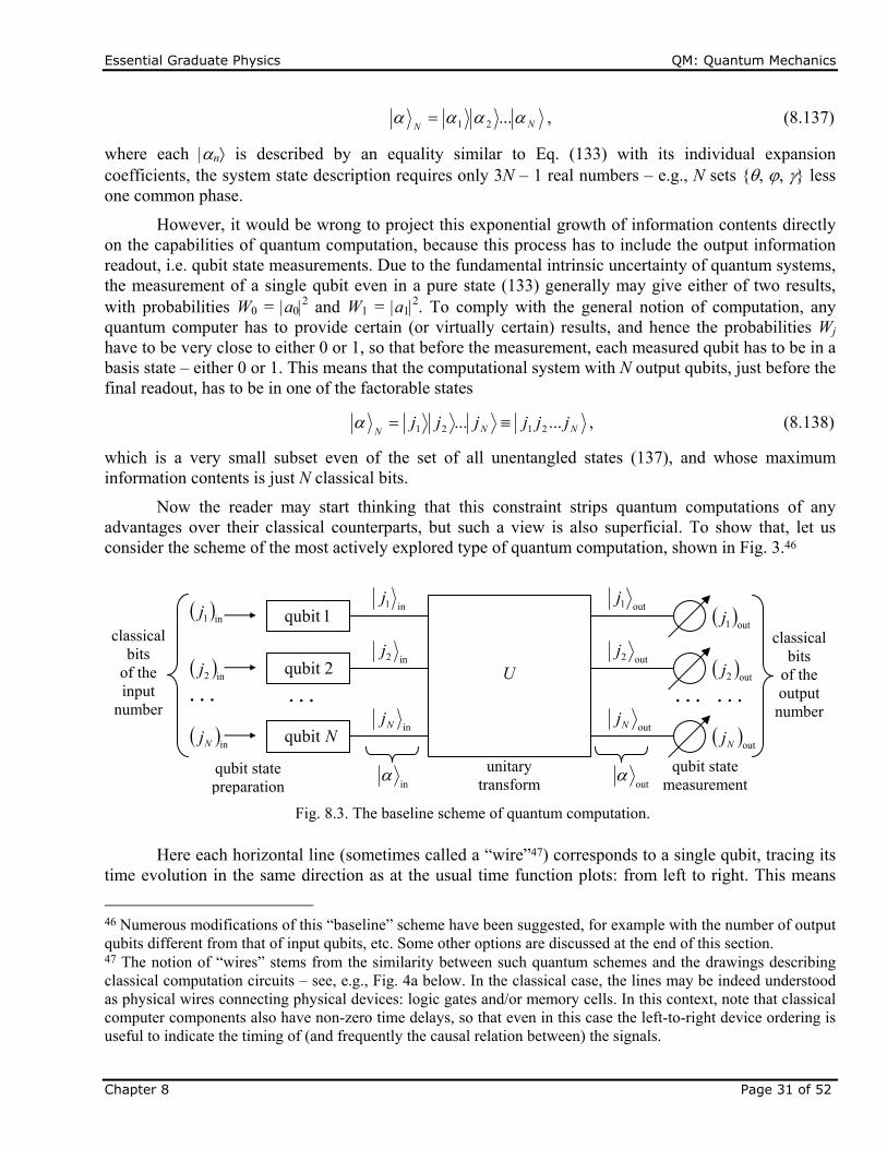
Essential Graduate Physics QM: Quantum Mechanics
Chapter 8 Page 31 of 52
NN ...21 , (8.137)
where each n is described by an equality similar to Eq. (133) with its individual expansion coefficients, the system state description requires only 3N – 1 real numbers – e.g., N sets {, , } less one common phase.
However, it would be wrong to project this exponential growth of information contents directly on the capabilities of quantum computation, because this process has to include the output information readout, i.e. qubit state measurements. Due to the fundamental intrinsic uncertainty of quantum systems, the measurement of a single qubit even in a pure state (133) generally may give either of two results, with probabilities W0 = a02 and W1 = a12. To comply with the general notion of computation, any quantum computer has to provide certain (or virtually certain) results, and hence the probabilities Wj have to be very close to either 0 or 1, so that before the measurement, each measured qubit has to be in a basis state – either 0 or 1. This means that the computational system with N output qubits, just before the final readout, has to be in one of the factorable states
NNNjjjjjj ...... 2121 , (8.138)
which is a very small subset even of the set of all unentangled states (137), and whose maximum information contents is just N classical bits.
Now the reader may start thinking that this constraint strips quantum computations of any advantages over their classical counterparts, but such a view is also superficial. To show that, let us consider the scheme of the most actively explored type of quantum computation, shown in Fig. 3.46
Here each horizontal line (sometimes called a “wire”47) corresponds to a single qubit, tracing its time evolution in the same direction as at the usual time function plots: from left to right. This means
46 Numerous modifications of this “baseline” scheme have been suggested, for example with the number of output qubits different from that of input qubits, etc. Some other options are discussed at the end of this section. 47 The notion of “wires” stems from the similarity between such quantum schemes and the drawings describing classical computation circuits – see, e.g., Fig. 4a below. In the classical case, the lines may be indeed understood as physical wires connecting physical devices: logic gates and/or memory cells. In this context, note that classical computer components also have non-zero time delays, so that even in this case the left-to-right device ordering is useful to indicate the timing of (and frequently the causal relation between) the signals.
Fig. 8.3. The baseline scheme of quantum computation.
in1j
in2jU
inNj
in
outunitary
transform
classical bits
of the output number
1qubit
qubit state preparation
classical bits
of the input
number
in1j
2qubit
Nqubit
in2j
inNj
out1j
out2j
outNj
out1j
out2j
outNj
qubit state measurement
Essential Graduate Physics QM: Quantum Mechanics
Chapter 8 Page 32 of 52
that the left column in of ket-vectors describes the initial state of the qubits,48 while the right column out describes their final (but pre-measurement) state. The box labeled U represents the qubit evolution in time due to their specially arranged interactions between each other and/or external drive “forces”. Besides these forces, during this evolution the system is supposed to be ideally isolated from the dephasing and energy-dissipating environment, so that the process may be described by a unitary operator defined in the 2N-dimensional Hilbert space of N qubits:
inout
ˆ U . (8.139)
With the condition that the input and output states have the simple form (138), this equality reads
inin2in1outout2out1 ... ˆ... NN jjjUjjj . (8.140)
The art of quantum computer design consists of selecting such unitary operators U that would:
- satisfy Eq. (140),
- be physically implementable, and
-enable substantial performance advantages of the quantum computation over its classical counterparts with similar functionality, at least for some digital functions (algorithms).
I will have time/space to demonstrate the possibility of such advantages on just one, perhaps the simplest example – the so-called Deutsch problem,49 on the way discussing several common notions and issues of this field. Let us consider the family of single-bit classical Boolean functions jout = f(jin). Since both j are Boolean variables, i.e. may take only values 0 and 1, there are evidently only 4 such functions – see the first four columns of the following table:
(8.141)
Of them, the functions f1 and f4, whose values are independent of their arguments, are called constants, while the functions f2 (called “YES” or “IDENTITY”) and f3 (“NOT” or “INVERSION”) are called balanced. The Deutsch problem is to determine the class of a single-bit function, implemented in a “black box”, as being either constant or balanced, using just one experiment.
48 As was discussed in Chapter 7, the preparation of a pure state (133) is (conceptually :-) straightforward. Placing a qubit into a weak contact with an environment of temperature T << /kB, where is the difference between energies of the eigenstates 0 and 1, we may achieve its relaxation into the lowest-energy state. Then, if the qubit must be set into a different pure state, it may be driven there by the application of a pulse of a proper external classical “force”. For example, if an actual spin-½ is used as the qubit, a pulse of a magnetic field, with proper direction and duration, may be applied to arrange its precession to the required Bloch sphere point – see Fig. 5.3c. However, in most physical implementations of qubits, a more practicable way for that step is to use a proper part of the Rabi oscillation period – see Sec. 6.5. 49 It is named after David Elieser Deutsch, whose 1985 paper (motivated by an inspirational but not very specific publication by Richard Feynman in 1982) launched the whole field of quantum computation.
f f(0) f(1) class F f(1)-f(0)
f1 0 0 constant 0 0
f2 0 1 balanced 1 1
f3 1 0 balanced 1 -1
f4 1 1 constant 0 0
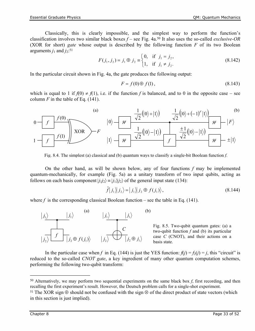
Essential Graduate Physics QM: Quantum Mechanics
Chapter 8 Page 33 of 52
Classically, this is clearly impossible, and the simplest way to perform the function’s classification involves two similar black boxes f – see Fig. 4a.50 It also uses the so-called exclusive-OR (XOR for short) gate whose output is described by the following function F of its two Boolean arguments j1 and j2:51
. if1,
, if0,),(
21
212121 jj
jjjjjjF (8.142)
In the particular circuit shown in Fig. 4a, the gate produces the following output:
)1()0( ffF , (8.143)
which is equal to 1 if f(0) f(1), i.e. if the function f is balanced, and to 0 in the opposite case – see column F in the table of Eq. (141).
On the other hand, as will be shown below, any of four functions f may be implemented quantum-mechanically, for example (Fig. 5a) as a unitary transform of two input qubits, acting as follows on each basis component j1j2 j1j2 of the general input state (134):
)(ˆ12121 jfjjjjf , (8.144)
where f is the corresponding classical Boolean function – see the table in Eq. (141).
In the particular case when f in Eq. (144) is just the YES function: f(j) = f2(j) = j, this “circuit” is reduced to the so-called CNOT gate, a key ingredient of many other quantum computation schemes, performing the following two-qubit transform:
50 Alternatively, we may perform two sequential experiments on the same black box f, first recording, and then recalling the first experiment’s result. However, the Deutsch problem calls for a single-shot experiment. 51 The XOR sign should not be confused with the sign of the direct product of state vectors (which in this section is just implied).
(a) (b)
Fig. 8.5. Two-qubit quantum gates: (a) a two-qubit function f and (b) its particular case C (CNOT), and their actions on a basis state.
f
1j
2j )( 12 jfj
1j
2j 12 jj
C
1j1j
(a) (b)
f
f
0
1
)0(f
)1(fF
Fig. 8.4. The simplest (a) classical and (b) quantum ways to classify a single-bit Boolean function f.
H
f
0
1
102
1
102
1 10
2
1
XOR
1102
1 F
F
1H
H
H
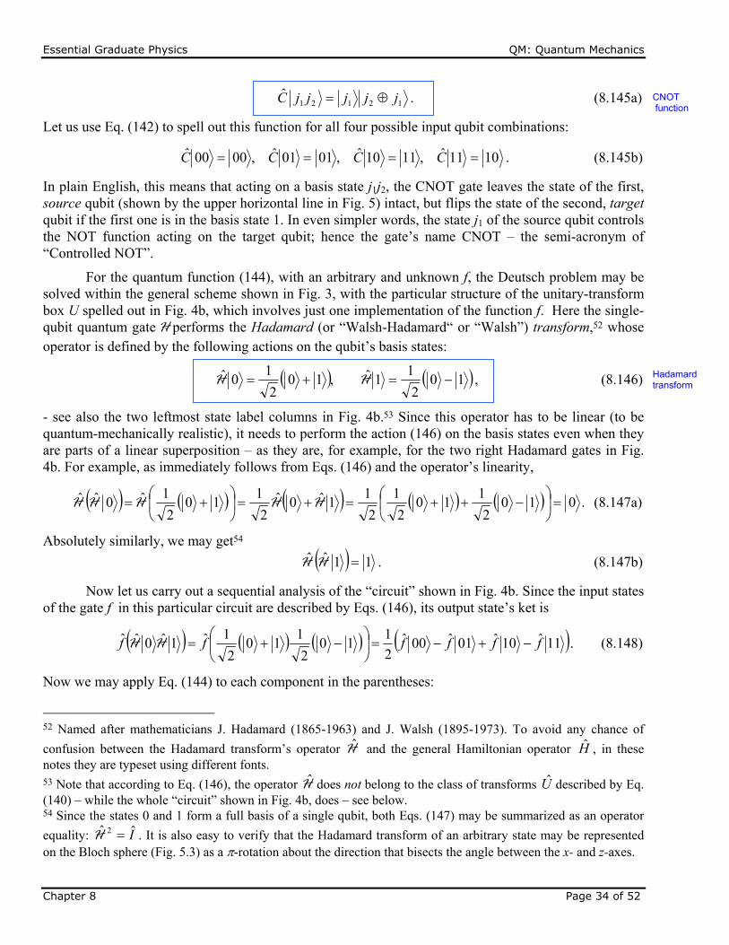
Essential Graduate Physics QM: Quantum Mechanics
Chapter 8 Page 34 of 52
12121ˆ jjjjjC . (8.145a)
Let us use Eq. (142) to spell out this function for all four possible input qubit combinations:
1011ˆ,1110ˆ,0101ˆ,0000ˆ CCCC . (8.145b)
In plain English, this means that acting on a basis state j1j2, the CNOT gate leaves the state of the first, source qubit (shown by the upper horizontal line in Fig. 5) intact, but flips the state of the second, target qubit if the first one is in the basis state 1. In even simpler words, the state j1 of the source qubit controls the NOT function acting on the target qubit; hence the gate’s name CNOT – the semi-acronym of “Controlled NOT”.
For the quantum function (144), with an arbitrary and unknown f, the Deutsch problem may be solved within the general scheme shown in Fig. 3, with the particular structure of the unitary-transform box U spelled out in Fig. 4b, which involves just one implementation of the function f. Here the single-qubit quantum gate H performs the Hadamard (or “Walsh-Hadamard“ or “Walsh”) transform,52 whose operator is defined by the following actions on the qubit’s basis states:
102
11ˆ,10
2
10ˆ HH , (8.146)
- see also the two leftmost state label columns in Fig. 4b.53 Since this operator has to be linear (to be quantum-mechanically realistic), it needs to perform the action (146) on the basis states even when they are parts of a linear superposition – as they are, for example, for the two right Hadamard gates in Fig. 4b. For example, as immediately follows from Eqs. (146) and the operator’s linearity,
.0102
110
2
1
2
11ˆ0ˆ
2
110
2
1ˆ0ˆˆ
HHHHH (8.147a)
Absolutely similarly, we may get54
11ˆˆ HH . (8.147b)
Now let us carry out a sequential analysis of the “circuit” shown in Fig. 4b. Since the input states of the gate f in this particular circuit are described by Eqs. (146), its output state’s ket is
11ˆ10ˆ01ˆ00ˆ2
110
2
110
2
1ˆ1ˆ0ˆˆ ffffff
HH . (8.148)
Now we may apply Eq. (144) to each component in the parentheses:
52 Named after mathematicians J. Hadamard (1865-1963) and J. Walsh (1895-1973). To avoid any chance of
confusion between the Hadamard transform’s operator H and the general Hamiltonian operator H , in these notes they are typeset using different fonts. 53 Note that according to Eq. (146), the operator H does not belong to the class of transforms U described by Eq. (140) – while the whole “circuit” shown in Fig. 4b, does – see below. 54 Since the states 0 and 1 form a full basis of a single qubit, both Eqs. (147) may be summarized as an operator
equality: Iˆ 2 H . It is also easy to verify that the Hadamard transform of an arbitrary state may be represented on the Bloch sphere (Fig. 5.3) as a -rotation about the direction that bisects the angle between the x- and z-axes.
CNOT function
Hadamard transform
Essential Graduate Physics QM: Quantum Mechanics
Chapter 8 Page 35 of 52
.)1(1)1(01)0(1)0(00
)1(11)1(01)0(10)0(00
11ˆ01ˆ10ˆ00ˆ11ˆ10ˆ01ˆ00ˆ
ffff
ffff
ffffffff
(8.149)
Note that the contents of the first parentheses of the last expression, characterizing the state of the target qubit, is equal to (0 – 1) (-1)0 (0 – 1) if f(0) = 0 (and hence 0f(0) = 0 and 1f(0) = 1), and to (1 – 0) (-1)1(0 – 1) in the opposite case f(0) = 1, so that both cases may be described in one shot by rewriting the parentheses as (-1)f(0)(0 – 1). The second parentheses is absolutely similarly controlled by the value of f(1), so that the outputs of the gate f are unentangled:
,102
11)1(0
2
1101)1(0)1(
2
11ˆ0ˆˆ )1()0( Ffff HH (8.150)
where the last step has used the fact that the classical Boolean function F, defined by Eq. (142), is equal to [f(1) – f(0)] – please compare the last two columns in Eq. (141). The front sign in Eq. (150) may be prescribed to any of the component ket-vectors – for example to that of the target qubit, as shown by the third column of state labels in Fig. 4b.
This intermediate result is already rather remarkable. Indeed, it shows that, despite the superficial impression one could get from Fig. 5, the gates f and C, being “controlled” by the source qubit, may change that qubit’s state as well! This fact (partly reflected by the vertical direction of the control lines in Figs. 4 and 5, symbolizing the same stage of the system’s time evolution) shows how careful one should be interpreting quantum-computational “circuits”, thriving on qubits’ entanglement, because the “signals” on different sections of a “wire” may differ – see Fig. 4b again.
At the last stage of the circuit shown in Fig. 4b, the qubit components of the state (150) are fed into one more pair of Hadamard gates, whose outputs therefore are
0ˆ1ˆ2
110
2
1ˆ and,1ˆ)1(0ˆ2
11)1(0
2
1ˆ HHHHHH
FF . (8.151)
Now using Eqs. (146) again, we see that the output state ket-vectors of the source and target qubits are, respectively,
1 and,12
)1(10
2
)1(1
FF
. (8.152)
Since, according to Eq. (142), the Boolean function F may take only values 0 or 1, the final state of the source qubit is always one of its basis states j, namely the one with j = F. Its measurement tells us whether the function f, participating in Eq. (144), is constant or balanced – see Eq. (141) again.55
Thus, the quantum circuit shown in Fig. 4b indeed solves the Deutsch problem in one shot. Reviewing our analysis, we may see that this is possible because the unitary transform performed by the quantum gate f is applied to the entangled states (146) rather than to the basis states. Due to this trick, the quantum state components depending on f(0) and f(1) are processed simultaneously, in parallel. This
55 Note that the last Hadamard transform of the target qubit (i.e. the Hadamard gate shown in the lower right corner of Fig. 4b) is not necessary for the Deutsch problem’s solution – though it should be included if we want the whole circuit to satisfy the condition (140).
Essential Graduate Physics QM: Quantum Mechanics
Chapter 8 Page 36 of 52
quantum parallelism may be extended to circuits with many (N >> 1) qubits and, for some tasks, provide a dramatic performance increase – for example, reducing the necessary circuit component number from O(2N) to O(N p), where p is a finite (and not very big) number.
However, this efficiency comes at a high price. Indeed, let us discuss the possible physical implementation of quantum gates, starting from the single-qubit case, on an example of the Hadamard gate (146). With the linearity requirement, its action on the arbitrary state (133) should be
,12
10
2
110
2
110
2
11ˆ0ˆˆ
10101010 aaaaaaaa HHH (8.153)
meaning that the state probability amplitudes in the end (t = T) and in the beginning (t = 0) of the qubit evolution in time have to be related as
.2
)0()0()(,
2
)0()0()( 10
110
0
aaa
aaa
TT (8.154)
This task may be again performed using the Rabi oscillations, which were discussed in Sec. 6.5, i.e. by applying to the qubit (a two-level system), for a limited time period T, a weak sinusoidal external
signal of frequency equal to the intrinsic quantum oscillation frequency nn’ defined by Eq. (6.85). The analysis of the Rabi oscillations was carried out in Sec. 6.5, even for non-vanishing (though small) detuning = – nn, but only for the particular initial conditions when at t = 0 the system was fully in one on the basis states (there labeled as n’), i.e. the counterpart state (there labeled n) was empty. For our current purposes we need to find the amplitudes a0,1(t) for arbitrary initial conditions a0,1(0), subject only to the time-independent normalization condition a02 + a12 = 1. For the case of exact tuning, = 0, the solution of the system (6.94) is elementary,56 and gives the following solution:57
,sin)0(cos)0()(
,sin)0(cos)0()(
011
100
teiatata
teiatatai
i
(8.155)
where is the Rabi oscillation frequency (6.99), in the exact-tuning case proportional to the amplitude A of the external ac drive A = Aexp{i} – see Eq. (6.86). Comparing these expressions with Eqs. (154), we see that for t = T = /4 and = /2 they “almost” coincide, besides the opposite sign of
a1(T). Conceptually the simplest way to correct this deficiency is to follow the ac “/4-pulse”, just
discussed, by a short dc “-pulse” of the duration T’ = /, which temporarily creates a small additional
energy difference between the basis states 0 and 1. According to the basic Eq. (1.62), such difference creates an additional phase difference T’/ between the states, equal to for the “-pulse”.
Another way (that may be also useful for two-qubit operations) is to use another, auxiliary energy level E2 whose distances from the basic levels E1 and E0 are significantly different from the difference (E1 – E0) – see Fig. 6a. In this case, the weak external ac field tuned to any of the three potential quantum transition frequencies nn’ (En- En’)/ initiates such transitions between the corresponding states only, with a negligible perturbation of the third state. (Such transitions may be
56 An alternative way to analyze the qubit evolution is to use the Bloch equation (5.21), with an appropriate function (t) describing the control field. 57 To comply with our current notation, the coefficients an’ and an of Sec. 6.5 are replaced with a0 and a1.
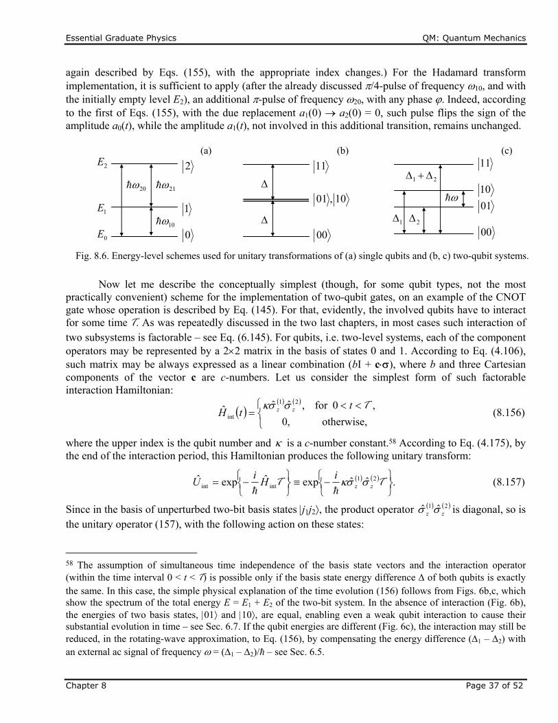
Essential Graduate Physics QM: Quantum Mechanics
Chapter 8 Page 37 of 52
again described by Eqs. (155), with the appropriate index changes.) For the Hadamard transform implementation, it is sufficient to apply (after the already discussed /4-pulse of frequency 10, and with the initially empty level E2), an additional -pulse of frequency 20, with any phase . Indeed, according to the first of Eqs. (155), with the due replacement a1(0) a2(0) = 0, such pulse flips the sign of the amplitude a0(t), while the amplitude a1(t), not involved in this additional transition, remains unchanged.
Now let me describe the conceptually simplest (though, for some qubit types, not the most practically convenient) scheme for the implementation of two-qubit gates, on an example of the CNOT gate whose operation is described by Eq. (145). For that, evidently, the involved qubits have to interact for some time T. As was repeatedly discussed in the two last chapters, in most cases such interaction of two subsystems is factorable – see Eq. (6.145). For qubits, i.e. two-level systems, each of the component operators may be represented by a 22 matrix in the basis of states 0 and 1. According to Eq. (4.106), such matrix may be always expressed as a linear combination (bI + c), where b and three Cartesian components of the vector c are c-numbers. Let us consider the simplest form of such factorable interaction Hamiltonian:
otherwise, ,0
,0for ,ˆˆˆ21
int
TttH zz
(8.156)
where the upper index is the qubit number and is a c-number constant.58 According to Eq. (4.175), by the end of the interaction period, this Hamiltonian produces the following unitary transform:
.ˆˆexpˆexpˆ 21intint
TT zz
iH
iU
(8.157)
Since in the basis of unperturbed two-bit basis states j1j2, the product operator 21 ˆˆ zz is diagonal, so is the unitary operator (157), with the following action on these states:
58 The assumption of simultaneous time independence of the basis state vectors and the interaction operator (within the time interval 0 < t < T) is possible only if the basis state energy difference of both qubits is exactly the same. In this case, the simple physical explanation of the time evolution (156) follows from Figs. 6b,c, which show the spectrum of the total energy E = E1 + E2 of the two-bit system. In the absence of interaction (Fig. 6b), the energies of two basis states, 01 and 10, are equal, enabling even a weak qubit interaction to cause their substantial evolution in time – see Sec. 6.7. If the qubit energies are different (Fig. 6c), the interaction may still be reduced, in the rotating-wave approximation, to Eq. (156), by compensating the energy difference (1 – 2) with an external ac signal of frequency = (1 – 2)/ – see Sec. 6.5.
Fig. 8.6. Energy-level schemes used for unitary transformations of (a) single qubits and (b, c) two-qubit systems.
0
1
2
0E
20 21
101E
2E
00
10,01
11
(a) (b) (c)
00
01
11
21
1021
Essential Graduate Physics QM: Quantum Mechanics
Chapter 8 Page 38 of 52
,expˆ21
)2()1(21int jjijjU zz (8.158)
where –T/, and z are the eigenvalues of the Pauli matrix z for the basis states of the
corresponding qubit: z = +1 for j = 0, and z = –1 for j = 1. Let me, for clarity, spell out Eq. (158) for the particular case = –/4 (corresponding to the qubit coupling time T = /4):
1111ˆ,1010ˆ,0101ˆ,0000ˆ 4/4/4/4/intintintint
iiii eUeUeUeU . (8.159)
In order to compensate the undesirable parts of this joint phase shift of the basis states, let us now apply similar individual “rotations” of each qubit by angle ’ = +/4, using the following product of two independent operators, plus (just for the result’s clarity) a common, and hence inconsequential, phase shift ” = –/4:59
4/2121com ˆ
4expˆ
4expˆˆexpˆ ieii"i'iU zzzz
. (8.160)
Since this operator is also diagonal in the j1j2 basis, it is easy to calculate the change of the basis states
by the total unitary operator intcomtotˆˆˆ UUU :
1111ˆ,1010ˆ,0101ˆ,0000ˆtottottottot UUUU . (8.161)
This result already shows the main “miracle action” of two-qubit gates, such as the one shown in Fig. 4b: the source qubit is left intact (only if it is in one of the basis states!), while the state of the target qubit is altered. True, this change (of the sign) is still different from the CNOT operator’s action (145), but may be readily used for its implementation by sandwiching of the transform Utot between two Hadamard transforms of the target qubit alone:
2tot
2 ˆˆˆ2
1ˆ HH UC . (8.162)
So, we have spent quite a bit of time on the discussion of the CNOT gate,60 and now I can reward the reader for their effort with a bit of good news: it has been proved that an arbitrary unitary transform that satisfies Eq. (140), i.e. may be used within the general scheme outlined in Fig. 3, may be decomposed into a set of CNOT gates, possibly augmented with simpler single-qubit gates – for example, the Hadamard gate plus the /2 rotation discussed above.61 Unfortunately, I have no time for a
59 As Eq. (4.175) shows, each of the component unitary transforms }ˆ'exp{ zi may be created by applying to
each qubit, for time interval T’ = ’/’, a constant external field described by Hamiltonian z'H ˆˆ . We
already know that for a charged, spin-½ particle, such Hamiltonian may be created by applying a z-oriented external dc magnetic field – see Eq. (4.163). For most other physical implementations of qubits, the organization of such a Hamiltonian is also straightforward – see, e.g., Fig. 7.4 and its discussion. 60 As was discussed above, this gate is identical to the two-qubit gate shown in Fig. 5a for f = f3, i.e. f(j) = j. The implementation of the gate of f for 3 other possible functions f requires straightforward modifications, whose analysis is left for the reader’s exercise. 61 This fundamental importance of the CNOT gate was perhaps a major reason why David Wineland, the leader of the NIST group that had demonstrated its first experimental implementation in 1995 (following the theoretical suggestion by J. Cirac and P. Zoller), was awarded the 2012 Nobel Prize in Physics – shared with Serge Haroche, the leader of another group working towards quantum computation.
Essential Graduate Physics QM: Quantum Mechanics
Chapter 8 Page 39 of 52
detailed discussion of more complex circuits.62 The most famous of them is the scheme for integer number factoring, suggested in 1994 by Peter Winston Shor.63 Due to its potential practical importance for breaking broadly used communication encryption schemes such as the RSA code,64 this opportunity has incited much enthusiasm and triggered experimental efforts to implement quantum gates and circuits using a broad variety of two-level quantum systems. By now, the following experimental options have given the most significant results:65
(i) Trapped ions. The first experimental demonstrations of quantum state manipulation (including the already mentioned first CNOT gate) have been carried out using deeply cooled atoms in optical traps, similar to those used in frequency and time standards. Their total spins are natural qubits, whose states may be manipulated using the Rabi transfers excited by suitably tuned lasers. The spin interactions with the environment may be very weak, resulting in large dephasing times T2 – up to a few seconds. Since the distances between ions in the traps are relatively large (of the order of a micron), their direct spin-spin interaction is even weaker, but the ions may be made effectively interacting either via their mechanical oscillations about the potential minima of the trapping field, or via photons in external electromagnetic resonators (“cavities”).66 Perhaps the main challenge of using this approach for quantum computation is poor “scalability”, i.e. the enormous experimental difficulty of creating and managing large ordered systems of individually addressable qubits. So far, only a-few-qubit systems have been demonstrated.67
(ii) Nuclear spins are also typically very weakly connected to their environment, with dephasing times T2 exceeding 10 seconds in some cases. Their eigenenergies E0 and E1 may be split by external dc magnetic fields (typically, of the order of 10 T), while the interstate Rabi transfers may be readily achieved by using the nuclear magnetic resonance, i.e. the application of external ac fields with frequencies = (E1 – E0)/ – typically, of a few hundred MHz. The challenges of this option include the weakness of spin-spin interactions (typically mediated through molecular electrons), resulting in a very slow spin evolution, whose time scale / may become comparable with T2, and also very small level separations E1 – E0, corresponding to a few K, i.e. much smaller than the room temperature, creating a challenge of qubit state preparation.68 Despite these challenges, the nuclear spin option was used for the first implementation of the Shor algorithm for factoring of a small number (15 = 53) as early as 2001.69 However, the extension of this success to larger systems, beyond the set of spins inside one molecule, is extremely challenging.
62 For that, the reader may be referred to either the monographs by Nielsen-Chuang and Reiffel-Polak, cited above, or to a shorter (but much more formal) textbook by N. Mermin, Quantum Computer Science, Cambridge U. Press, 2007. 63 A clear description of this algorithm may be found in several accessible sources, including Wikipedia – see the article Shor’s Algorithm. 64 Named after R. Rivest, A. Shamir, and L. Adleman, the authors of the first open publication of the code in 1977, but actually invented earlier (in 1973) by C. Cocks. 65 For a discussion of other possible implementations (such as quantum dots and dopants in crystals) see, e.g., T. Ladd et al., Nature 464, 45 (2010), and references therein. 66 A brief discussion of such interactions (so-called Cavity QED) will be given in Sec. 9.4 below. 67 See, e.g., S. Debnath et al., Nature 536, 63 (2016). Note also the related work on arrays of trapped, optically-coupled neutral atoms – see, e.g., J. Perczel et al., Phys. Rev. Lett. 119, 023603 (2017) and references therein. 68 This challenge may be partly mitigated using ingenious spin manipulation techniques such as refocusing – see, e.g., either Sec. 7.7 in Nielsen and Chuang, or the J. Keeler’s monograph cited at the end of Sec. 6.5. 69 B. Lanyon et al., Phys. Rev. Lett. 99, 250505 (2001).
Essential Graduate Physics QM: Quantum Mechanics
Chapter 8 Page 40 of 52
(iii) Josephson-junction devices. Much better scalability may be achieved with solid-state devices, especially using superconductor integrated circuits including weak contacts – Josephson junctions (see their brief discussion in Sec. 1.6). The qubits of this type are based on the fact that the energy U of such a junction is a highly nonlinear function of the Josephson phase difference – see Sec. 1.6. Indeed, combining Eqs. (1.73) and (1.74), we can readily calculate U() as the work W of an external circuit increasing the phase from, say, zero to some value :
cos1
2sin
20 cc
0'00
eIdt
dt
'd'
eIIVdtdUU
''
'
'
'W . (8.163)
There are several options of using this nonlinearity for creating qubits;70 currently the leading option, called the phase qubit, is using two lowest eigenstates localized in one of the potential wells of the periodic potential (163). A major problem of such qubits is that at the very bottom of this well the potential U() is almost quadratic, so that the energy levels are nearly equidistant – cf. Eqs. (2.262), (6.16), and (6.23). This is even more true for the so-called “transmons” (and “Xmons”, and “Gatemons”, and several other very similar devices71) – the currently used phase qubits versions, where a Josephson junction is made a part of an external electromagnetic oscillator, making its relative total nonlineartity (anharmonism) even smaller. As a result, the external rf drive of frequency = (E1 – E0)/, used to arrange the state transforms described by Eq. (155), may induce simultaneous undesirable transitions to (and between) higher energy levels. This effect may be mitigated by a reduction of the ac drive amplitude, but at a price of the proportional increase of the operation time and hence of dephasing – see below. (I am leaving a quantitative estimate of such an increase for the reader’s exercise.)
Since the coupling of Josephson-junction qubits may be most readily controlled (and, very importantly, kept stable if so desired), they have been used to demonstrate the largest prototype quantum computing systems to date, despite quite modest dephasing times T2 – for purely integrated circuits, in the tens of microseconds at best, even at operating temperatures in tens of mK. By the time of this writing (mid-2019), several groups have announced chips with a few dozen of such qubits, but to the best of my knowledge, only their smaller subsets could be used for high-fidelity quantum operations.72
(iv) Optical systems, attractive because of their inherently enormous bandwidth, pose a special challenge for quantum computation: due to the virtual linearity of most electromagnetic media at reasonable light power, the implementation of qubits (i.e. two-level systems), and interaction Hamiltonians such as the one given by Eq. (156), is problematic. In 2001, a very smart way around this
70 The “most quantum” option in this technology is to use Josephson junctions very weakly coupled to their dissipative environment (so that the effective resistance shunting the junction is much higher than the quantum
resistance unit RQ (/2) /e2 ~ 104 ). In this case, the Josephson phase variable behaves as a coordinate of a 1D quantum particle, moving in the 2-periodic potential (163), forming the energy band structure E(q) similar to those discussed in Sec. 2.7. Both theory and experiment show that in this case, the quantum states in adjacent Brillouin zones differ by the charge of one Cooper pair 2e. (This is exactly the effect responsible for the Bloch oscillations of frequency (2.252).) These two states may be used as the basis states of charge qubits. Unfortunately, such qubits are rather sensitive to charged impurities, randomly located in the junction’s vicinity, causing uncontrollable changes of its parameters, so that currently, to the best of my knowledge, this option is not actively pursued. 71 For a recent review of these devices see, e.g., G. Wendin, Repts. Progr. Phys. 80, 106001 (2017), and references therein. 72 See, e.g., C. Song et al., Phys. Rev. Lett. 119, 180511 (2017) and references therein.
Essential Graduate Physics QM: Quantum Mechanics
Chapter 8 Page 41 of 52
hurdle was invented.73 In this KLM scheme (also called the “linear optical quantum computing”), nonlinear elements are not needed at all, and quantum gates may be composed just of linear devices (such as optical waveguides, mirrors, and beam splitters), plus single-photon sources and detectors. However, estimates show that this approach requires a much larger number of physical components than those using nonlinear quantum systems such as usual qubits,74 so that right now it is not very popular.
So, despite more than two decades of large-scale efforts, the progress of quantum computing development has been rather modest. The main culprit here is the unintentional coupling of qubits to their environment, leading most importantly to their state dephasing, and eventually to errors. Let me discuss this major issue in detail.
Of course, some error probability exists in classical digital logic gates and memory cells as well.75 However, in this case, there is no conceptual problem with the device state measurement, so that the error may be detected and corrected in many ways. Conceptually,76 the simplest of them is the so-called majority voting logic – using several similar logic circuits working in parallel and fed with identical input data. Evidently, two such devices can detect a single error in one of them, while three devices in parallel may correct such error, by taking two coinciding output signals for the genuine one.
For quantum computation, the general idea of using several devices (say, qubits) for coding the same information remains valid; however, there are two major complications. First, as we know from Chapter 7, the environment’s dephasing effect may be described as a slow random drift of the probability amplitudes aj, leading to the deviation of the output state fin from the required form (140), and hence to a non-vanishing probability of wrong qubit state readout – see Fig. 3. Hence the quantum error correction has to protect the result not against possible random state flips 0 1, as in classical digital computers, but against these “creeping” analog errors.
Second, the qubit state is impossible to copy exactly (clone) without disturbing it, as follows from the following simple calculation.77 Cloning some state of one qubit to another qubit that is initially in an independent state (say, the basis state 0), without any change of , means the following transformation of the two-qubit ket: 0 . If we want such transform to be performed by a real quantum system, whose evolution is described by a unitary operator u , and to be correct for an arbitrary state , it has to work not only for both basis states of the qubit:
,1110ˆ,0000ˆ uu (8.164)
but also for their arbitrary linear combination (133). Since the operator u has to be linear, we may use that relation, and then Eq. (164) to write
73 E. Knill et al., Nature 409, 46 (2001). 74 See, e.g., Y. Li et al., Phys. Rev. X 5, 041007 (2015). 75 In modern integrated circuits, such “soft” (runtime) errors are created mostly by the high-energy neutron component of cosmic rays, and also by the -particles emitted by radioactive impurities in silicon chips and their packaging. 76 Practically, the majority voting logic increases circuit complexity and power consumption, so that it is used only in most critical points. Since in modern digital integrated circuits the bit error rate is very small (< 10-5), in most of them, less radical but also less penalizing schemes are used – if used at all. 77 Amazingly, this simple no-cloning theorem was discovered as late as 1982 (to the best of my knowledge, independently by W. Wooters and W. Zurek, and by D. Dieks), in the context of work toward quantum cryptography – see below.
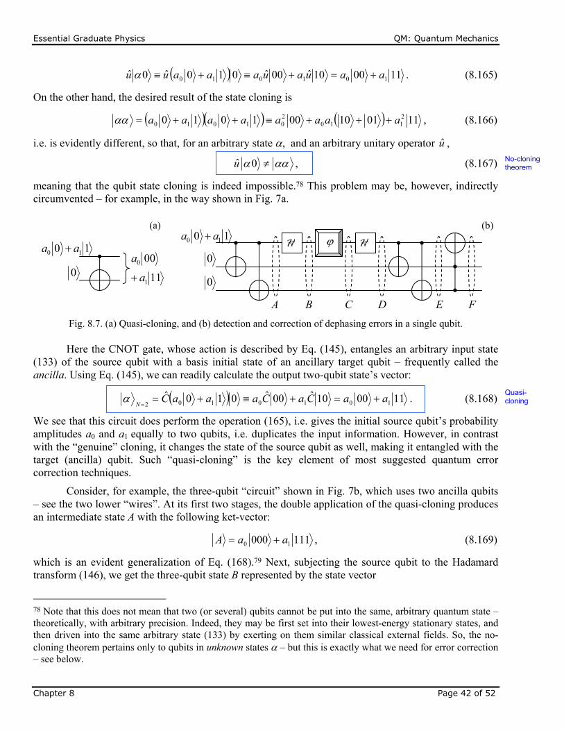
Essential Graduate Physics QM: Quantum Mechanics
Chapter 8 Page 42 of 52
110010ˆ00ˆ010ˆ0ˆ 101010 aauauaaauu . (8.165)
On the other hand, the desired result of the state cloning is
110110001010 2110
201010 aaaaaaaa , (8.166)
i.e. is evidently different, so that, for an arbitrary state , and an arbitrary unitary operator u ,
0u , (8.167)
meaning that the qubit state cloning is indeed impossible.78 This problem may be, however, indirectly circumvented – for example, in the way shown in Fig. 7a.
Here the CNOT gate, whose action is described by Eq. (145), entangles an arbitrary input state (133) of the source qubit with a basis initial state of an ancillary target qubit – frequently called the ancilla. Using Eq. (145), we can readily calculate the output two-qubit state’s vector:
110010ˆ00ˆ010ˆ1010102
aaCaCaaaCN
. (8.168)
We see that this circuit does perform the operation (165), i.e. gives the initial source qubit’s probability amplitudes a0 and a1 equally to two qubits, i.e. duplicates the input information. However, in contrast with the “genuine” cloning, it changes the state of the source qubit as well, making it entangled with the target (ancilla) qubit. Such “quasi-cloning” is the key element of most suggested quantum error correction techniques.
Consider, for example, the three-qubit “circuit” shown in Fig. 7b, which uses two ancilla qubits – see the two lower “wires”. At its first two stages, the double application of the quasi-cloning produces an intermediate state A with the following ket-vector:
111000 10 aaA , (8.169)
which is an evident generalization of Eq. (168).79 Next, subjecting the source qubit to the Hadamard transform (146), we get the three-qubit state B represented by the state vector
78 Note that this does not mean that two (or several) qubits cannot be put into the same, arbitrary quantum state – theoretically, with arbitrary precision. Indeed, they may be first set into their lowest-energy stationary states, and then driven into the same arbitrary state (133) by exerting on them similar classical external fields. So, the no-cloning theorem pertains only to qubits in unknown states – but this is exactly what we need for error correction – see below.
Quasi- cloning
No-cloning theorem
Fig. 8.7. (a) Quasi-cloning, and (b) detection and correction of dephasing errors in a single qubit.
(a) (b)
10 10 aa
0 11
00
1
0
a
a
0
0
H 10 10 aa
FEDCBA
H
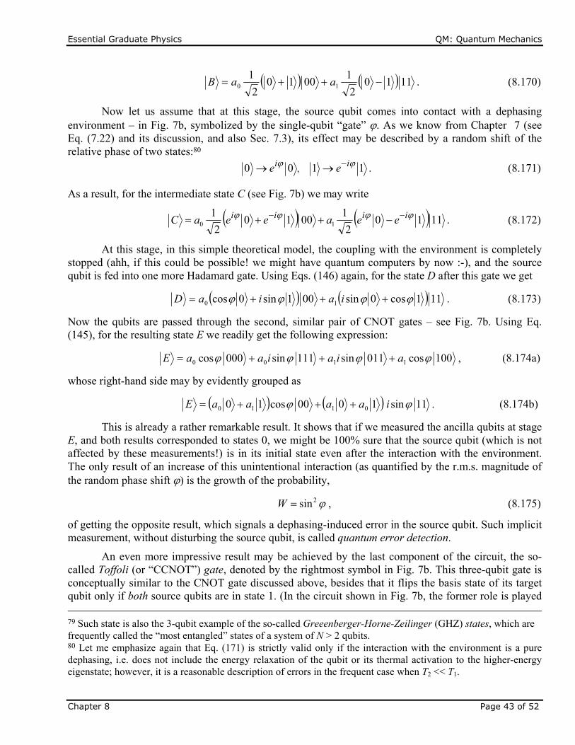
Essential Graduate Physics QM: Quantum Mechanics
Chapter 8 Page 43 of 52
11102
10010
2
110 aaB . (8.170)
Now let us assume that at this stage, the source qubit comes into contact with a dephasing environment – in Fig. 7b, symbolized by the single-qubit “gate” . As we know from Chapter 7 (see Eq. (7.22) and its discussion, and also Sec. 7.3), its effect may be described by a random shift of the relative phase of two states:80
1100 , ii ee . (8.171)
As a result, for the intermediate state C (see Fig. 7b) we may write
11102
10010
2
110
iiii eeaeeaC . (8.172)
At this stage, in this simple theoretical model, the coupling with the environment is completely stopped (ahh, if this could be possible! we might have quantum computers by now :-), and the source qubit is fed into one more Hadamard gate. Using Eqs. (146) again, for the state D after this gate we get
111cos0sin001sin0cos 10 iaiaD . (8.173)
Now the qubits are passed through the second, similar pair of CNOT gates – see Fig. 7b. Using Eq. (145), for the resulting state E we readily get the following expression:
100cos011sin111sin000cos 1100 aiaiaaE , (8.174a)
whose right-hand side may by evidently grouped as
11sin1000cos10 0110 iaaaaE . (8.174b)
This is already a rather remarkable result. It shows that if we measured the ancilla qubits at stage E, and both results corresponded to states 0, we might be 100% sure that the source qubit (which is not affected by these measurements!) is in its initial state even after the interaction with the environment. The only result of an increase of this unintentional interaction (as quantified by the r.m.s. magnitude of the random phase shift ) is the growth of the probability,
2sinW , (8.175)
of getting the opposite result, which signals a dephasing-induced error in the source qubit. Such implicit measurement, without disturbing the source qubit, is called quantum error detection.
An even more impressive result may be achieved by the last component of the circuit, the so-called Toffoli (or “CCNOT”) gate, denoted by the rightmost symbol in Fig. 7b. This three-qubit gate is conceptually similar to the CNOT gate discussed above, besides that it flips the basis state of its target qubit only if both source qubits are in state 1. (In the circuit shown in Fig. 7b, the former role is played
79 Such state is also the 3-qubit example of the so-called Greeenberger-Horne-Zeilinger (GHZ) states, which are frequently called the “most entangled” states of a system of N > 2 qubits. 80 Let me emphasize again that Eq. (171) is strictly valid only if the interaction with the environment is a pure dephasing, i.e. does not include the energy relaxation of the qubit or its thermal activation to the higher-energy eigenstate; however, it is a reasonable description of errors in the frequent case when T2 << T1.
Essential Graduate Physics QM: Quantum Mechanics
Chapter 8 Page 44 of 52
by our source qubit, while the latter role, by the two ancilla qubits.) According to its definition, the Toffoli gate does not affect the first parentheses in Eq. (174b), but flips the source qubit’s states in the second parentheses, so that for the output three-qubit state F we get
11sin1000cos10 1010 iaaaaF . (8.176a)
Obviously, this result may be factored as
11sin00cos10 10 iaaF , (8.176b)
showing that now the source qubit is again fully unentangled from the ancilla qubits. Moreover, calculating the norm squared of the second operand, we get
1sincos11sin00cos11sin00cos 22 ii , (8.177)
so that the final state of the source qubit exactly coincides with its initial state. This is the famous miracle of quantum state correction, taking place “automatically” – without any qubit measurements, and for any random phase shift .
The circuit shown in Fig. 7b may be further improved by adding Hadamard gate pairs, similar to that used for the source qubit, to the ancilla qubits as well. It is straightforward to show that if the dephasing is small in the sense that the W given by Eq. (175) is much less than 1, this modified circuit may provide a substantial error probability reduction (to ~W2) even if the ancilla qubits are also subjected to a similar dephasing and the source qubits, at the same stage – i.e. between the two Hadamard gates. Such perfect automatic correction of any error (not only of an inner dephasing of a qubit and its relaxation/excitation, but also of the mutual dephasing between qubits) of any used qubit needs even more parallelism. The first circuit of that kind, based on nine parallel qubits, which is a natural generalization of the circuit discussed above, was invented in 1995 by the same P. Shor. Later, five-qubit circuits enabling similar error correction were suggested. (The further parallelism reduction has been proved impossible.)
However, all these results assume that the error correction circuits as such are perfect, i.e. completely isolated from the environment. In the real world, this cannot be done. Now the key question is what maximum level Wmax of the error probability in each gate (including those in the used error correction scheme) can be automatically corrected, and how many qubits with W < Wmax would be required to implement quantum computers producing important practical results – first of all, factoring of large numbers.81 To the best of my knowledge, estimates of these two related numbers have been made only for some very specific approaches, and they are rather pessimistic. For example, using the so-called surface codes, which employ many physical qubits for coding an informational one, and hence increase its fidelity, Wmin may be increased to a few times 10-3, but then we would need ~108 physical qubits for the Shor’s algorithm implementation.82 This is very far from what currently looks doable using the existing approaches.
Because of this hard situation, the current development of quantum computing is focused on finding at least some problems that could be within the reach of either the existing systems, or their immediate extensions, and simultaneously would present some practical interest – a typical example of a
81 In order to compete with the existing classical factoring algorithms, such numbers should have at least 103 bits. 82 A. Fowler et al., Phys. Rev. A 86, 032324 (2012).
Quantum error correction
Essential Graduate Physics QM: Quantum Mechanics
Chapter 8 Page 45 of 52
technology in the search for applications. Currently, to the best of my knowledge, all suggested problems of this kind address either specially crafted mathematical problems,83 or properties of some simple physical systems – such as the molecular hydrogen84 or the deuteron (the deuterium’s nucleus, i.e. the proton-neutron system).85 In the latter case, the interaction between the qubits of the computational system is organized so that the system’s Hamiltonian is similar to that of the quantum system of interest. (For this work, quantum simulation is a more adequate name than “quantum computation”.86)
Such simulations are pursued by some teams using schemes different from that shown in Fig. 3. Of those, the most developed is the so-called adiabatic quantum computation,87 which drops the hardest requirement of negligible interaction with the environment. In this approach, the qubit system is first prepared in a certain initial state, and then is let evolve on its own, with no effort to couple-uncouple qubits by external control signals during the evolution.88 Due to the interaction with the environment, in particular the dephasing and the energy dissipation it imposes, the system eventually relaxes to a final incoherent state, which is then measured. (This reminds the scheme shown in Fig. 3, with the important difference that the transform U should not necessarily be unitary.) From numerous runs of such an experiment, the outcome statistics may be revealed. Thus, at this approach the interaction with the environment is allowed to play a certain role in the system evolution, though every effort is made to reduce it, thus slowing down the relaxation process – hence the word “adiabatic” in the name of this approach. This slowness allows the system to exhibit some quantum properties, in particular quantum tunneling89 through the energy barriers separating close energy minima in the multi-dimensional space of states. This tunneling creates a substantial difference in the finite state statistics from that in purely classical systems, where such barriers may be overcome only by thermally-activated jumps over them.90
Due to technical difficulties of the organization and precise control of long-range interaction in multi-qubit systems, the adiabatic quantum computing demonstrations so far have been limited to a few simple arrays described by the so-called extended quantum Ising (“spin-glass”) model
j
jzj
jj
jz
jz σhσσJH ˆˆˆˆ
}',{
' , (8.178)
where the curly brackets denote the summation over pairs of close (though not necessarily closest) neighbors. Though the Hamiltonian (178) is the traditional playground of phase transitions theory (see,
83 F. Arute et al., Nature 574, 505 (2019). Note that the claim of the first achievement of “quantum supremacy”, made in this paper, refers only to an artificial, specially crafted mathematical problem, and does not change my assessment of the current status of this technology. 84 P. O’Malley et al., Phys. Rev. X 6, 031007 (2016). 85 E. Dumitrescu et al., Phys. Lett. Lett. 120, 210501 (2018). 86 To the best of my knowledge, this idea was first put forward by Yuri I. Malin in his book Computable and Incomputable published in 1980, i.e. before the famous 1982 paper by Richard Feynman. Unfortunately, since the book was in Russian, this suggestion was acknowledged by the international community only much later. 87 Note that the qualifier “quantum” is important in this term, to distinguish this research direction from the classical adiabatic (or “reversible”) computation – see, e.g., SM Sec. 2.3 and references therein. 88 Recently, some hybrids of this approach with the “usual” scheme of quantum computation have been demonstrated, in particular, using some control of inter-bit coupling during the relaxation process – see, e.g., R. Barends et al., Nature 534, 222 (2016). 89 As a reminder, this process was repeatedly discussed in this course, starting from Sec. 2.3. 90 A quantitative discussion of such jumps may be found in SM Sec. 5.6.
Essential Graduate Physics QM: Quantum Mechanics
Chapter 8 Page 46 of 52
e.g., SM Chapter 4), to the best of my knowledge there are not many practically important tasks that could be achieved by studying the statistics of its solutions. Moreover, even for this limited task, the speed of the largest experimental adiabatic quantum “computers”, with several hundreds of Josephson-junction qubits91 is still comparable with that of classical, off-the-shelf semiconductor processors (with the dollar cost lower by many orders of magnitude), and no dramatic change of this comparison is predicted for realistic larger systems.
To summarize the current (circa mid-2019) situation with the quantum computation development, it faces a very hard challenge of mitigating the effects of unintentional coupling with the environment. This problem is exacerbated by the lack of algorithms, beyond Shor’s factoring, that would give quantum computation a substantial advantage over the classical competition in solving real-world problems, and hence a much broader potential customer base that would provide the field with the necessary long-term motivation and resources. So far, even the leading experts in this field abstain from predictions on when quantum computation may become a self-supporting commercial technology.92
There seem to be somewhat better prospects for another application of entangled qubit systems, namely to telecommunication cryptography.93 The goal here is more modest: to replace the currently dominating classical encryption, based on the public-key RSA code mentioned above, that may be broken by factoring very large numbers, with a quantum encryption system that would be fundamentally unbreakable. The basis of this opportunity is the measurement postulate and the no-cloning theorem: if a message is carried over by a qubit, it is impossible for an eavesdropper (in cryptography, traditionally called Eve) to either measure or copy it faithfully, without also disturbing its state. However, as we have seen from the discussion of Fig. 7a, state quasi-cloning using entangled qubits is possible, so that the issue is far from being simple, especially if we want to use a publicly distributed quantum key, in some sense similar to the classical public key used at the RSA encryption. Unfortunately, I would not have time/space to discuss various options for quantum encryption, but cannot help demonstrating how counter-intuitive they may be, on the famous example of the so-called quantum teleportation (Fig. 8).94
Suppose that some party A (in cryptography, traditionally called Alice) wants to send to party B (Bob) the full information about the pure quantum state of a qubit, unknown to either party. Instead of sending her qubit directly to Bob, Alice asks him to send her one qubit () of a pair of other qubits, prepared in a certain entangled state, for example in the singlet state described by Eq. (11); in our current notation
10012
1' . (8.179)
The initial state of the whole three-qubit system may be represented in the form
91 See, e.g., R. Harris et al., Science 361, 162 (2018). Similar demonstrations with trapped-ion systems so far have been on a smaller scale, with a few tens of qubits – see, e.g., J. Zhang et al., Nature 551, 601 (2017). 92 See the publication Quantum Computing: Progress and Prospects, The National Academies Press, 2019. 93 This field was pioneered in the 1970s by S. Wisener. Its important theoretical aspect (which I, unfortunately, also will not be able to cover) is the distinguishability of different but close quantum states – for example, of an original qubit set, and that slightly corrupted by noise. A good introduction to this topic may be found, for example, in Chapter 9 of the monograph by Nielsen and Chuang, cited above. 94 This procedure had been first suggested in 1993 by Charles Henry Bennett, and then repeatedly demonstrated experimentally – see, e.g., L. Steffen et al., Nature 500, 319 (2013), and literature therein.
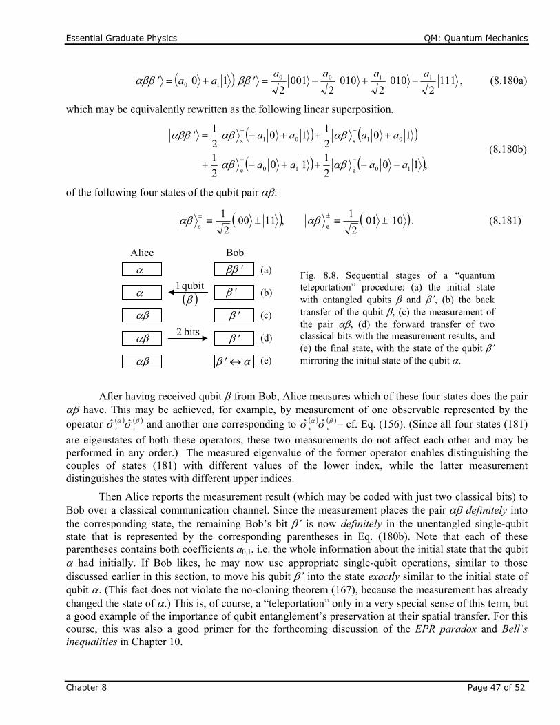
Essential Graduate Physics QM: Quantum Mechanics
Chapter 8 Page 47 of 52
1112
0102
0102
0012
10 110010
aaaa'aa' , (8.180a)
which may be equivalently rewritten as the following linear superposition,
,102
110
2
1
102
110
2
1
10e10e
01s01s
aaaa
aaaa'
(8.180b)
of the following four states of the qubit pair :
10012
1,1100
2
1es
. (8.181)
After having received qubit from Bob, Alice measures which of these four states does the pair have. This may be achieved, for example, by measurement of one observable represented by the operator zz ˆˆ and another one corresponding to xx ˆˆ – cf. Eq. (156). (Since all four states (181)
are eigenstates of both these operators, these two measurements do not affect each other and may be performed in any order.) The measured eigenvalue of the former operator enables distinguishing the couples of states (181) with different values of the lower index, while the latter measurement distinguishes the states with different upper indices.
Then Alice reports the measurement result (which may be coded with just two classical bits) to Bob over a classical communication channel. Since the measurement places the pair definitely into the corresponding state, the remaining Bob’s bit ’ is now definitely in the unentangled single-qubit state that is represented by the corresponding parentheses in Eq. (180b). Note that each of these parentheses contains both coefficients a0,1, i.e. the whole information about the initial state that the qubit had initially. If Bob likes, he may now use appropriate single-qubit operations, similar to those discussed earlier in this section, to move his qubit ’ into the state exactly similar to the initial state of qubit . (This fact does not violate the no-cloning theorem (167), because the measurement has already changed the state of .) This is, of course, a “teleportation” only in a very special sense of this term, but a good example of the importance of qubit entanglement’s preservation at their spatial transfer. For this course, this was also a good primer for the forthcoming discussion of the EPR paradox and Bell’s inequalities in Chapter 10.
'
'
'
'bits 2
'
Fig. 8.8. Sequential stages of a “quantum teleportation” procedure: (a) the initial state with entangled qubits and ’, (b) the back transfer of the qubit , (c) the measurement of the pair , (d) the forward transfer of two classical bits with the measurement results, and (e) the final state, with the state of the qubit ’ mirroring the initial state of the qubit .
(a)
(b)
(c)
(d)
(e)
Alice Bob
qubit 1
Essential Graduate Physics QM: Quantum Mechanics
Chapter 8 Page 48 of 52
Returning for just a minute to quantum cryptography: since its most common quantum key distribution protocols95 require just a few simple quantum gates, whose experimental implementation is not a large technological challenge, the main focus of the current effort is on decreasing the single-photon dephasing in long electromagnetic-wave transmission channels,96 with sufficiently high qubit transfer fidelity. The recent progress was rather impressive, with the demonstrated transfer of entangled qubits over landlines longer than 100 km,97 and over at least one satellite-based line longer than 1,000 km;98 and also the whole quantum key distribution over a comparable distance, though for now at a very low rate yet.99 Let me hope that if not the author of this course, then its readers will see this technology used in practical secure telecommunication systems.
8.6. Exercise problems
8.1. Prove that Eq. (30) indeed yields Eg(1) = (5/4)EH.
8.2. For a dilute gas of helium atoms in their ground state, with n atoms per unit volume, calculate its:
(i) electric susceptibility e, and (ii) magnetic susceptibility m,
and compare the results.
Hint: You may use the model solution of Problems 6.8 and 6.14, and the results of the variational description of the helium atom’s ground state in Sec. 2. 8.3. Calculate the expectation values of the following observables: s1s2, S
2 (s1 + s2)2, and Sz
s1z + s2z, for the singlet and triplet states of the system of two spins-½, defined by Eqs. (18) and (21), directly, without using the general Eq. (48). Compare the results with those for the system of two classical geometric vectors of length /2 each. 8.4. Discuss the factors 1/2 that participate in Eqs. (18) and (20) for the entangled states of the system of two spins-½, in terms of Clebsh-Gordan coefficients similar to those discussed in Sec. 5.7. 8.5.* Use the perturbation theory to calculate the contribution into the so-called hyperfine splitting of the ground energy of the hydrogen atom,100 due to the interaction between the spins of its nucleus (proton) and electron.
95 Two of them are the BB84 suggested in 1984 by C. Bennett and G. Brassard, and the EPRBE suggested in 1991 by A. Ekert. For details, see, e.g., either Sec. 12.6 in the repeatedly cited monograph by Nielsen and Chuang, or the review by N. Gizin et al., Rev. Mod. Phys. 74, 145 (2002). 96 For their quantitative discussion see, e.g., EM Sec. 7.8. 97 See, e.g., T. Herbst et al., Proc. Nath. Acad. Sci. 112, 14202 (2015), and references therein. 98 J. Yin et al., Science 356, 1140 (2017). 99 H.-L. Yin et al., Phys. Rev. Lett. 117, 190501 (2016). 100 This effect was discovered experimentally by A. Michelson in 1881 and explained theoretically by W. Pauli in 1924.
Essential Graduate Physics QM: Quantum Mechanics
Chapter 8 Page 49 of 52
Hint: The proton’s magnetic moment operator is described by the same Eq. (4.115) as the electron, but with a positive gyromagnetic factor p = gpe/2mp 2.675108 s-1T-1, whose magnitude is much smaller than that of the electron (e 1.7611011 s-1T-1), due to the much higher mass, mp 1.67310-27 kg 1,835 me. (The g-factor of the proton is also different, gp 5.586.101) 8.6. In the simple case of just two similar spin-interacting particles, distinguishable by their spatial location, the famous Heisenberg model of ferromagnetism102 is reduced to the following Hamiltonian:
2121 ˆˆˆˆ ssss BJH ,
where J is the spin interaction constant, is the gyromagnetic ratio of each particle, and B is the external magnetic field. Find the stationary states and energies of this system for spin-½ particles. 8.7. Two particles, both with spin-½ but different gyromagnetic ratios 1 and 2, are placed to external magnetic field B. In addition, their spins interact as in the Heisenberg model:
21int ˆˆˆ ss JH .
Find the eigenstates and eigenenergies of the system. 8.8. Two similar spin-½ particles, with gyromagnetic ratio , localized at two points separated by distance a, interact via the field of their magnetic dipole moments. Calculate stationary states and energies of the system.
8.9. Consider the permutation of two identical particles, each of spin s. How many different symmetric and antisymmetric spin states can the system have?
8.10. For a system of two identical particles with s = 1:
(i) List all spin states forming the uncoupled-representation basis. (ii) List all possible pairs {S, MS} of the quantum numbers describing the states of the coupled- representation basis – see Eq. (48). (iii)Which of the {S, MS} pairs describe the states symmetric, and which the states antisymmetric, with respect to the particle permutation? 8.11. Represent the operators of the total kinetic energy and the total orbital angular momentum of a system of two particles, with masses m1 and m2, as combinations of terms describing the center-of-mass motion and the relative motion. Use the results to calculate the energy spectrum of the so-called
101 The anomalously large value of the proton’s g-factor results from the composite quark-gluon structure of this particle. (An exact calculation of gp remains a challenge for quantum chromodynamics.) 102 It was suggested in 1926, independently by W. Heisenberg and P. Dirac. A discussion of thermal motion effects on this and other similar systems (especially the Ising model of ferromagnetism) may be found in SM Chapter 4.
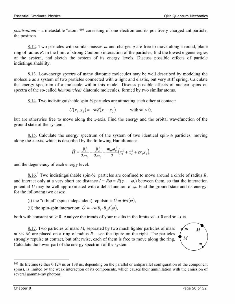
Essential Graduate Physics QM: Quantum Mechanics
Chapter 8 Page 50 of 52
positronium – a metastable “atom”103 consisting of one electron and its positively charged antiparticle, the positron. 8.12. Two particles with similar masses m and charges q are free to move along a round, plane ring of radius R. In the limit of strong Coulomb interaction of the particles, find the lowest eigenenergies of the system, and sketch the system of its energy levels. Discuss possible effects of particle indistinguishability. 8.13. Low-energy spectra of many diatomic molecules may be well described by modeling the molecule as a system of two particles connected with a light and elastic, but very stiff spring. Calculate the energy spectrum of a molecule within this model. Discuss possible effects of nuclear spins on spectra of the so-called homonuclear diatomic molecules, formed by two similar atoms. 8.14. Two indistinguishable spin-½ particles are attracting each other at contact:
0,with ,, 2121 WW xxxxU
but are otherwise free to move along the x-axis. Find the energy and the orbital wavefunction of the ground state of the system.
8.15. Calculate the energy spectrum of the system of two identical spin-½ particles, moving
along the x-axis, which is described by the following Hamiltonian:
2122
21
200
0
22
0
21
22
ˆ
2
ˆˆ xxxxm
m
p
m
pH
,
and the degeneracy of each energy level. 8.16.* Two indistinguishable spin-½ particles are confined to move around a circle of radius R, and interact only at a very short arc distance l = R R(1 – 2) between them, so that the interaction potential U may be well approximated with a delta function of . Find the ground state and its energy, for the following two cases:
(i) the “orbital” (spin-independent) repulsion: WU ,
(ii) the spin-spin interaction: 21 ˆˆˆ ss WU ,
both with constant W > 0. Analyze the trends of your results in the limits W 0 and W . 8.17. Two particles of mass M, separated by two much lighter particles of mass m << M, are placed on a ring of radius R – see the figure on the right. The particles strongly repulse at contact, but otherwise, each of them is free to move along the ring. Calculate the lower part of the energy spectrum of the system.
103 Its lifetime (either 0.124 ns or 138 ns, depending on the parallel or antiparallel configuration of the component spins), is limited by the weak interaction of its components, which causes their annihilation with the emission of several gamma-ray photons.
M
M
m
m
Essential Graduate Physics QM: Quantum Mechanics
Chapter 8 Page 51 of 52
8.18. N indistinguishable spin-½ particles move in a spherically-symmetric quadratic potential U(r) = m0
2r2/2. Neglecting the direct interaction of the particles, find the ground-state energy of the system. 8.19. Use the Hund rules to find the values of the quantum numbers L, S, and J in the ground states of the atoms of carbon and nitrogen. Write down the Russell-Saunders symbols for these states. 8.20. N >> 1 indistinguishable, non-interacting quantum particles are placed in a hard-wall, rectangular box with sides ax, ay, and az. Calculate the ground-state energy of the system, and the average forces it exerts on each face of the box. Can we characterize the forces by certain pressure P?
Hint: Consider separately the cases of bosons and fermions. 8.21.* Explore the Thomas-Fermi model104 of a heavy atom, with the nuclear charge Q = Ze >> e, in which the interaction between electrons is limited to their contribution to the common electrostatic potential (r). In particular, derive the ordinary differential equation obeyed by the radial distribution of the potential, and use it to estimate the effective radius of the atom. 8.22.* Use the Thomas-Fermi model, explored in the previous problem, to calculate the total binding energy of a heavy atom. Compare the result with that for the simpler model, in that the Coulomb electron-electron interaction is completely ignored. 8.23. A system of three similar spin-½ particles is described by the Heisenberg Hamiltonian (cf. Problems 6 and 7):
133221 ˆˆˆˆˆˆˆ ssssss JH ,
where J is the spin interaction constant. Find the stationary states and energies of this system, and give an interpretation of your results. 8.24. For a system of three spins-½, find the common eigenstates and eigenvalues of the
operators zS and 2S , where
321 ˆˆˆˆ sssS
is the vector operator of the total spin of the system. Do the corresponding quantum numbers S and MS obey Eqs. (48)? 8.25. Explore basic properties of the Heisenberg model (which was the subject of Problems 6, 7, and 23), for a 1D chain of N spins-½:
,0with ,ˆˆˆˆ
',' JJH
jj
jjjj sss B
where the summation is over all N spins, with the symbol {j, j’} meaning that the first sum is only over the adjacent spin pairs. In particular, find the ground state of the system and its lowest excited states in the absence of external magnetic field B, and also the dependence of their energies on the field.
104 It was suggested in 1927, independently, by L. Thomas and E. Fermi.
Essential Graduate Physics QM: Quantum Mechanics
Chapter 8 Page 52 of 52
Hint: For the sake of simplicity, you may assume that the first sum includes the term 1ˆˆ ss N as
well. (Physically, this means that the chain is bent into a closed loop. 105) 8.26. Compose the simplest model Hamiltonians, in terms of the second quantization formalism,
for systems of indistinguishable particles moving in the following external potentials:
(i) two weakly coupled potential wells, with on-site particle interactions (giving additional energy J per each pair of particles in the same potential well), and (ii) a periodic 1D potential, with the same particle interactions, in the tight-binding limit.
8.27. For each of the Hamiltonians composed in the previous problem, derive the Heisenberg
equations of motion for particle creation/annihilation operators:
(i) for bosons, and (ii) for fermions.
8.28. Express the ket-vectors of all possible Dirac states for the system of three indistinguishable
(i) bosons, and (ii) fermions,
via those of the single-particle states , ’, and ” they occupy. 8.29. Explain why the general perturbative result (8.126), when applied to the 4He atom, gives the correct106 expression (8.29) for the ground singlet state, and correct Eqs. (8.39)-(8.42) (with the minus sign in the first of these relations) for the excited triplet states, but cannot describe these results, with the plus sign in Eq. (8.39), for the excited singlet state. 8.30. For a system of two distinct qubits (i.e. two-level systems), introduce a reasonable uncoupled-representation z-basis, and write in this basis the 44 matrix of the operator that swaps their states.
8.31. Find a time-independent Hamiltonian that can cause the qubit evolution described by Eqs. (155). Discuss the relation between your result and the time-dependent Hamiltonian (6.86).
105 Note that for dissipative spin systems, differences between low-energy excitations of open-end and closed-end 1D chains may be substantial even in the limit N – see, e.g., SM Sec. 4.5. However, for our Hamiltonian (and hence dissipation-free) system, the differences are relatively small. 106 Correct in the sense of the first order of the perturbation theory.
Related Documents