CHAPTER 8 FACTOR EXTRACTION BY MATRIX …rcm/book/ch8.pdf · 180 CHAPTER 8 FACTOR EXTRACTION BY MATRIX FACTORING TECHNIQUES From Exploratory Factor Analysis Ledyard R Tucker and Robert

180

CHAPTER 8FACTOR EXTRACTION BY MATRIX FACTORING TECHNIQUES

FromExploratory Factor Analysis

Ledyard R Tuckerand

Robert C. MacCallum

©1997

181

CHAPTER 8

FACTOR EXTRACTION BY MATRIX FACTORING TECHNIQUES

In this chapter we delve into a number of intricacies of factor extraction by matrix

factoring techniques. These methods are the older ones followed in many early studies when

there were considerable computation limitations. These methods were developed prior to the

advent of large scale computers. However, some of the techniques were not utilized due to the

computing requirements but were considered as highly desirable. With modern computers these

methods are quite feasible. For a general framework in considering the factor extraction

techniques we refer to Guttman's (1944) general theory and methods for matrix factoring which

provides a theoretic foundation for the matrix factoring techniques which had been in use or had

been being considered for some time. The methods to be considered in this chapter maximize

some function of the obtained factor loadings. Consideration of residuals is only tangential. Two

areas of problems are closely related to the factor extraction procedures, these are: the problem of

"guessed communalities" and the problem of number of factors to be extracted. After

presentation of the general theory of matrix factoring, a section will discuss the subject of

"guessed communalities". Determination of the number of factors appears to be closely related to

the method of factor extraction and will be discussed with each such technique.

Before discussion of details of matrix factoring techniques there are several preliminary

matters to be considered. These techniques are not scale free when applied to covariance matrices

in general in that results vary with scaling of the attributes. The property of a factor extraction

technique being scale free may be explained in reference to the following equations. Let be an�

original covariance matrix to which a scaling diagonal matrix is applied, being finite,� �

positive, non-singular. Let be the rescaled covariance matrix.��

� � ��

� �

A selected factor extraction technique is applied to to yield a common factor matrix which� ��

is scaled back to for the original covariance matrix by:�c

� � ��

For the factor extraction technique to be scale free, matrix must be invariant with use of�c

different scaling matrices . As is well known, a correlation matrix is independent of the�

scaling of a covariance matrix.

� � � ��

��

where

182

� ��

� � ��

�

Note that:

� � ��

A common factor matrix obtained from may be scaled back to and by:� � ��

��

� � � ��

� � ��

In order to avoid scaling problems we follow the tradition of applying these techniques to

correlation matrices. In a sense, this usage does make these techniques scale free when the

obtained factor matrix may be scaled back to apply to the original attribute scales.

For notational convenience, the subscripts of the observed correlation matrix are��

dropped so that the observed correlation matrix is indicated by . Also, matrix will be� ��

indicated by . Equation (7.17) becomes:�

� ��

This is the basic equation considered in this chapter. An alternative equation is obtained by

defining matrix with adjusted diagonal entries with "guessed communalities" by:��

� � � � ��

From equation (8.1):

� � ��

� ��

Matrix contains residual correlations. Several letters used in transformations of factors will be�

used in the present context on a temporary basis to designate other matrices in this chapter.

8.1. General Theory of Matrix Factoring

Guttman (1944) developed a general theory of matrix factoring with which he described

several existing methods of factor extraction. This theory applies, strictly in the present context,

to Gramian matrices. These matrices need not be of full rank; however, for the present purposes

they must not have imaginary dimensions (the least eigenvalue must be non-negative). A

correlation matrix satisfies these conditions since it is the product of a score matrix times its

transpose, an original definition of a Gramian matrix. Usually, however, matrix with adjusted��

183

diagonal entries containing "guessed communalities" is not Gramian. Nevertheless, the theory of

matrix factoring is applied to matrix In practice, with a few exceptions, this use appears to�� .

work satisfactorily.

The general procedure starts from a Gramian matrix which is and of rank ,G� n n r�

greater than 0 and equal to or less than A matrix , with greater than 0 and equaln n m. � � m

to or less than . is to contain real numbers and satisfy a restriction stated later. Matrix isn � �

defined by:

� � � ��

Note that is . Matrix , , is defined by:� n m m m� ��

� � � � � ��

Matrix is Gramian and must be of full rank; this is the restriction on matrix . A square� �

decomposition matrix is determined such that:�

��

Any of several techniques may be used to determine . A section of a factor matrix, , on� n m�

orthogonal axes is defined by:

� � ��

and a residual matrix is defined by:��

� � � ��

� ��

There is a dual problem of proof. First, that the rank of is ( - ) . Second, that is a�� r m ��

section with columns of a complete, orthogonal factor matrix of .m ��

The required proofs are expedited by considering a complete decomposition of to a��

matrix , , such that:� n r�

��

� is a factor matrix on orthogonal axes and can be obtained by any of a number of procedures

such as the procedure developed by Commandant A. L. Cholesky of the French Navy around

1915 and described by Dwyer (1944) as the square root method. There are many other possible

procedures to obtain this decomposition. With equation (8.9), matrices and become:� �

� � ��

� � ��

184

Then, matrix becomes:.��

� � ��

Define a matrix , :�� r � m

� � � ��

Then, matrix �� becomes:

� � ��

Matrix is column wise orthonormal as shown by the following:��

� � � � ��

� � ��

� ��

�

� �

� ��

��

��

�

�

�

� ��

Matrix , orthonormal, is completed by adjoining section , to .� � �r r r� �� ( )r m�

� � ��

� �� is column wise orthonormal and orthogonal by columns to . Matrix is rotated�

orthogonally by to yield matrix with sections and � � � �� .

��

Since is an orthonormal rotation and from equation (8.9):�

� � ��

� ��

Then with equation (8.8):

� � ��

��

Matrix is of rank ( ). The derivation of has removed this section from the complete�� r m� ��

matrix . This completes the needed proof.�

A point of interest is that is orthogonal to as shown as follows.� ��

� � ��

� �

Note, from equation (8.7), that:

� � � ��

� ��

185

With the results of equation (8.21), equation (8.20) becomes:

� � � � ��

� ��

�

� ��

��

� �

� �

� ��

A second point of interest is the relation between matrix and the obtained factor weight�

matrix From equations (8.5), (8.6), and (8.7)�� .

�

�

��

�

�

�

� ��

��

��

��

��

��

�

�

� ��

This result is important in the factor extraction methods.

Equations (8.4) through (8.8) are the bases of major steps in the factor extraction

techniques to be considered in this chapter. These methods differ in the determination of matrix

� �. Each of these techniques starts with a correlation matrix , having adjusted diagonal�1

entries, determines a weight matrix , computes a section of a factor matrix then computes� �� ,

a residual matrix by equation (8.8). This process is repeated with the residual matrix to��2

obtain the next section of the extracted factor matrix. This process is repeated with the

succession of residual matrices until the full extracted factor matrix is obtained. As indicated

earlier, the number of factors to be extracted is a decision frequently made from information

obtained during the factor extraction process. The basis of this decision depends on the factor

extraction technique employed.

8.2. The "Guessed Communalities" Problem

A preliminary operation in matrix factoring is to establish entries in the diagonals of the

correlation matrix. The theory of common factor analysis presented in the preceding chapters

establishes a basis for this operation. Note that the principal components procedure ignores the

issue of common vs. unique variance and leaves unities in the diagonal of the correlation matrix.

An early operational procedure using communality type values was the "Highest R" technique

developed by Thurstone (1947) and was used in many of his studies as well as by many other

individuals following Thurstone's lead. However, early in applications of digital computers there

was a proposal to use principal components as an easy approximation to factor analysis. Kaiser

(1960) described such a technique followed by VARIMAX transformation of the weight matrix.

This procedure, which became known as the "Little Jiffy" after a suggestion by Chester Harris, is

retained as an alternative in a number of computer packages. We can not recommend this

186

procedure and are concerned that many unwary individuals have been misled by the ease of

operations. Serious problems exist.

A very simple example is presented in Table 8.1 with the constructed correlation matrix

being given at the upper left. This correlation matrix was computed from a single common factor

with uniqueness so that the theoretic communalities were known and have been inserted into the

matrix on the upper right. There are neither sampling nor lack of fit discrepancies. A principal

components analysis is given on the left and a principal factors analysis is given on the right. The

principal factors procedure will be considered later in detail. For the principal components

analysis an eigen solution (see Appendix A on matrix algebra for a discussion of the eigen

problem) was obtained of the correlation matrix having unities in the diagonal. The series of

eigenvalues are given on the left along with the component weights for one dimension. These

weights are the entries in the first eigenvector times the square root of the first eigenvalue. The

matrix of residuals after removing this first component is given at the bottom left. The principal

factors analysis followed the same procedure as the principal components analysis but is applied

to the correlation matrix having communalities in the diagonal. For the principal factors, both the

weights for one factor and the uniqueness are given. These are the values used in constructing the

correlation matrix.

There are a number of points to note. First, the eigenvalues for the principal components

after the first value do not vanish as do the corresponding eigenvalues for the principal factors

analysis. If one followed the procedure for the principal components of retaining only dimensions

for which eigenvalues were greater than unity, only the first principal component would be used,

this being the number of dimensions used in this example. For the principal factors analysis, only

one factor existed since there was only one eigenvalue that did not vanish. A more important

comparison concerns the obtained weights. All of the principal component weights are greater

than the corresponding principal factor weights. This is especially true for the low to medium

sized weights. Use of the principal components procedure exaggerates the values of the obtained

weights. A further comparison is provided by the residual matrices. For the principal components

analysis on the left, the diagonal values might be taken to be unique variances (a common

interpretation). However, note the negative residuals. The component weights have removed too

much from the correlations leaving a peculiar residual structure. For the principal factors

analysis, all of the residual entries vanish in this example. The principal factors analysis yields a

proper representation of the correlation matrix. A conclusion from this example is that leaving

unities in the diagonals of a correlation matrix leads to a questionable representation of the

structure of the correlation matrix.

Tables 8.2 and 8.3 provide a comparison when lack of fit is not included and is included

in a constructed correlation matrix. The correlation matrix in Table 8.2 was computed from the

187

Table 8.1

Comparison of factor Extraction from a Correlation Matrix with Unities in the Diagonal

versus Communalities in the Diagonal

Correlation Matrices

Unities in Diagonal (RW1) Communalities in Diagonal (RWH)1 2 3 4 1 2 3 4

1 1.00 .35 .21 .07 1 .49 .35 .21 .072 .35 1.00 .15 .05 2 .35 .25 .15 .053 .21 .15 1.00 .03 3 .21 .15 .09 .034 .07 .05 .03 1.00 4 .07 .05 .03 .01

Eigenvalues of (RW1) Eigenvalues of (RWH)1 1.50 1 .842 .99 2 .003 .87 3 .004 .64 4 .00

Principal Components Principal FactorsWeights Weights Uniqueness

1 .78 1 .70 .512 .73 2 .50 .753 .56 3 .30 .914 .22 4 .10 .99

Residual Matrix from (RW1) Residual Matrix from (RWH)1 2 3 4 1 2 3 4

1 .40 -.22 -.23 -.10 1 .00 .00 .00 .002 -.22 .46 -.26 -.11 2 .00 .00 .00 .003 -.23 -.26 .69 -.09 3 .00 .00 .00 .004 -.10 -.11 -.09 .95 4 .00 .00 .00 .00

188

Table 8.2Illustration of “Communality” Type Values

Simulated Correlation matrix without Discrepancies of Fit

Major Domain Matrix Variance Components1 2 Major Unique Minor

1 .8 .0 .64 .36 .002 .6 .0 .36 .64 .003 .5 .1 .26 .74 .004 .2 .3 .13 .87 .005 .0 .2 .04 .96 .006 .0 .6 .36 .64 .00

Simulated Population Correlation Matrix1 2 3 4 5 6

1 1.002 .48 1.003 .40 .30 1.004 .16 .12 .13 1.005 .00 .00 .02 .06 1.006 .00 .00 .06 .18 .12 1.00

“Communality” Type Values

Attribute Method 1 2 3 4 5 6Major Domain Variance .64 .36 .26 .13 .04 .36Highest R .48 .48 .40 .18 .12 .18Squared Multiple Correlation .31 .25 .18 .07 .02 .05Iterated Centroid Factors .64 .36 .26 .13 .04 .36Iterated Principal Factors .64 .36 .26 .13 .04 .36Alpha Factor Analysis .64 .36 .26 .13 .04 .36Unrestricted Maximum Likelihood .64 .36 .26 .13 .04 .36

189

Table 8.3Illustration of “Communality” Type Values

simulated Correlation matrix without Discrepancies of Fit

Major Domain Matrix Variance Components1 2 Major Unique Minor

1 .8 .0 .64 .36 .102 .6 .0 .36 .54 .103 .5 .1 .26 .64 .104 .2 .3 .13 .77 .105 .0 .2 .04 .86 .106 .0 .6 .36 .54 .10

Simulated Population Correlation Matrix1 2 3 4 5 6

1 1.002 .49 1.003 .37 .28 1.004 .17 .16 .15 1.005 -.04 -.02 .03 .02 1.006 -.03 .02 .07 .21 .10 1.00

“Communality” Type Values

Attribute Method 1 2 3 4 5 6Major Domain Variance .64 .36 .26 .13 .04 .36Highest R .49 .49 .37 .21 .10 .21Squared Multiple Correlation .31 .25 .16 .09 .01 .06Iterated Centroid Factors .67 .36 .23 .12 .01 .73Iterated Principal Factors .65 .37 .23 .15 .02 .50Alpha Factor Analysis .69 .37 .23 .11 .02 .63Unrestricted Maximum Likelihood .65 .37 .23 .16 .02 .45

190

major domain matrix and the listed uniqueness. This is a perfect population correlation matrix. In

contrast, the technique described in Chapter 3, section 3.9, was used to add lack of fit

discrepancies to the generated correlation matrix given in Table 8.3. The bottom section of each

of these tables presents communality type values determined by a number of techniques.

Discussion will compare results by these techniques between the cases when there are no

discrepancies of fit and when there are discrepancies of fit.

Consider the case in Table 8.2 when no discrepancies of fit were included. The first row

in the bottom section contains the major domain variances which may be considered as theoretic

communalities. The second and third rows contain communality type values used in factor

extraction techniques. These will be discussed in subsequent paragraphs. The last four rows give

results from four methods of factor extraction which should result in ideal communalities in the

population. These methods will be discussed in detail in subsequent sections. All four of these

techniques utilize iterative computing methods to arrive at stable determinations of

communalities. Note that all four techniques are successful in arriving at the theoretic values

given in the row for the major domain variances. If a correlation matrix were determined from a

sample of individuals from a population characterized by a given population matrix which does

not include discrepancies of fit, an objective of factor extraction from this sample correlation

matrix would be to arrive at estimates of the major domain variances.

Consider the case in Table 8.3 when discrepancies of fit were included. As before, the

first row in the bottom section contains the major domain variances which, as will be

demonstrated, no longer can be considered as theoretic communalities. As before, the second and

third rows contain communality type values used in factor extraction techniques and will be

discussed subsequently. The last four rows give results for this case from four methods of factor

extraction which will be discussed in detail in subsequent sections. The values in these rows not

only vary from the values in Table 8.2 but also differ between methods of factor extraction. Note,

especially the values for attribute 6 for which the communality type values for the four methods

of factor extraction vary from .73 to .45 and are all greater than the .36 in Table 8.2. Inclusion of

the discrepancies of fit has had an effect on these values which is different for different methods

of factor extraction. There no longer is a single ideal solution. The population communalities

differ by method of factor extraction and provide different objectives to be estimated from

sample correlation matrices. This conclusion poses a considerable problem for statistical

modeling which ignores discrepancies of fit. We conclude that ignoring discrepancies of fit is

quite unrealistic and raises questions concerning several factoring techniques. This is an

illustration of the discussion in Chapter 3 of the effects of lack of fit on results obtained by

different methods of fitting the factor model.

8.2.1. Highest R Procedure

191

Thurstone developed the highest R procedure during the analyses of large experimental

test batteries such as in his study of Primary Mental Abilities (1938). Computations were

performed using mechanical desk calculators so that a simple procedure was needed which

would yield values in the neighborhood of what might be considered as the most desirable

values. The highest R technique is based on intuitive logic; there is no overall developmental

justification.

Application of the highest R technique involves, for each attribute, , finding the otherj

attribute, , which correlates most highly in absolute value with . This correlation, in absolute i j

value, is taken as a communality type value for attribute This procedure is illustrated in Tablej.

8.4. The correlation matrix in this table is the same as in Table 8.3 with reversals of directions of

attributes 3 and 5. In making these reversals of directions, algebraic signs are reversed in rows

and columns for these two attributes. Note that there are double reversals for the diagonal entries

and the correlation between the two attributes which results in no sign changes for these entries.

Consider the column for attribute 1. Ignore the diagonal entry and find the largest other entry in

absolute value. This value is .49 in row 2 and is recorded in the "Highest R" row. Note that for

column 3 the highest value in absolute value is .37, this is the -.37 in row 1. The foregoing

procedure is followed for each of the attributes. Note that the sign changes in the correlation

matrix between Tables 8.3 and 8.4 did not change the values of the highest R's.

Justification of the highest R technique rests mostly on the idea that attributes for which

communality type values should be high should correlate more highly with other attributes in a

battery than would be true for attributes for which the communality type values should be low.

This relation should be more nearly true for larger sized batteries of attributes than for smaller

sized batteries such as used in the illustration.

There are a few algebraic relations to be considered. Consider two attributes, and .i j

From equation (8.1) when there are no discrepancies of fit the correlation between these two

attributes is:

� � � � ��

This correlation can be expressed in trigonometric terms as the scalar product between two

vectors.

� � � � ��

where h and h are the lengths of these two vectors and is the cosine of the angle between� � ��

these two vectors. When the absolute value of the correlation is considered, as required in the

highest R procedure:

192

Table 8.4Illustration of “Highest R”

Correlation Matrix 1 2 3 4 5 6

1 1.002 .49 1.003 -.37 -.28 1.004 .17 .16 -.15 1.005 .04 .02 .03 -.02 1.006 -.03 .02 -.07 .21 -.10 1.00

Highest R .49 .49 .37 .21 .10 .21

193

� � � ��

When the two attribute vectors are collinear

� ��

so that

� ��

If the two attribute vectors have equal length,

� � ��

and

� ��

Thus, in this special case would yield the desired communality type values. In case the two� ��

vectors are not of equal length, such as:

� � ��

then:

� � � � ��

��

so that is too low for one of the h 's and too high for the other. When the two attribute� ��

vectors are not collinear

� ��

and there is a tendency for to be less the desired communality type values. The selection of� ��

attribute value will tend toward having a value1 to have a high correlation in absolute � ��

approaching unity.

8.2.2. Squared Multiple Correlations (SMC)'s

The "squared multiple correlation", or SMC, is the most commonly used communality

type value used in factor extraction procedures. This coefficient is the squared multiple

correlation for an attribute in a multiple, linear regression of that attribute with all otherj

attributes in a battery. Roff (1936) followed by Dwyer (1939) and Guttman (1940) showed that,

in perfect cases, the communality of an attribute was equal to or greater than the SMC for that

attribute. These developments presumed that the common factor model fit the correlation matrix

precisely (there was no lack of fit) and that a population matrix was considered (there were no

sampling discrepancies). Dwyer used a determinantal derivation while Guttman used super

194

matrices. We follow the Guttman form in our developments of this proposition. Guttman (1956)

described the SMC's as the "best possible" systematic estimates of communalities; a conclusion

justified in terms of a battery of attributes increasing indefinitely without increasing the number

of common factors. Following this development, the SMC became widely adopted and

incorporated into computer packages.

Standard procedures for computation of the SMC will be considered first. Initially, the

case is to be considered when the correlation matrix is nonsingular. This case should cover the

majority of factor analytic studies. Each attribute is considered in turn as a dependent variable

with the remaining ( - 1) attributes being considered as a battery of independent attributes. An

linear regression is considered relating attribute to the battery of independent attributes with thej

smc being the squared multiple correlation in this regression. The variance of the discrepancies�

between the observed values of and regressed values is designated by s . From regressionj ��

theory:

��

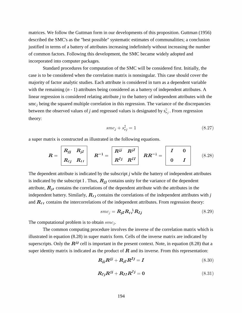
a super matrix is constructed as illustrated in the following equations.

� � ��

� � � �

� �

� �

� �

��

The dependent attribute is indicated by the subscript while the battery of independent attributesj

is indicated by the subscript I . Thus, unity for the variance of the dependent� contains

attribute, contains the correlations of the dependent attribute with the attributes in the�

independent battery. Similarly, contains the correlations of the independent attributes with � j

and contains the intercorrelations of the independent attributes. From regression theory:�

��

The computational problem is to obtain .��

The common computing procedure involves the inverse of the correlation matrix which is

illustrated in equation (8.28) in super matrix form. Cells of the inverse matrix are indicated by

superscripts. Only the cell is important in the present context. Note, in equation (8.28) that a�

super identity matrix is indicated as the product of and its inverse. From this representation:�

� � � � � � � ��

� � � � � � � ��

195


� � � � ��

� �

which yields which may be substituted into equation (8.30) to obtain:�

� � � � � � ��

� �

This equation may be solved to yield the desired equation for :�

� � � � � ��

� � � � ��

Equations for other cells of the inverse matrix may be obtained by similar solutions when

desired. With equation (8.29) equation (8.32) becomes:

� ��

��

so that:

��

An alternative involves :��

� � � � ��

This equation is obtained from (8.27) and (8.34) with being substituted for its equivalent�

unity in (8.27).

Equation (8.34) is extended to involving all attributes in the battery by defining diagonal

matrix containing the as the diagonal elements. Equation (8.34) may be expanded to:��

� ��

� ��

� ��

To adjust the diagonal elements of to having the SMC's , matrix must be subtracted from� ��

�

� in accordance to equation (8.27). Let be the correlation matrix with the SMC's in the��

diagonal cells.

� � ��

��

The two preceding equation provide the basis for computations.

There is trouble in applying the preceding procedure when the correlation matrix is

singular since, in this case, the inverse does not exist. A simple modification of this procedure

was suggested by Finkbeiner and Tucker (1982). A small positive number, k , is to be added to

each diagonal entry of to yield a matrix � ��

.

� � � ��

��

196

Define:

� ��

� ��

� ��

and compute by:��

� �

� ��

� � ��

�

� � �8.39

Two statements of approximation follow. As k approaches zero:

� ��

� approaches �

�;

approaches � ��

� � � � .

Finkbeiner and Tucker suggested a value of k = .000001 with which discrepancies in the

approximations were in the fourth decimal place.

The advantage of the Finkbeiner and Tucker modification is that when is a true�

Gramian matrix but is singular due to inclusion of dependent attributes in the battery, matrix ��

is not singular so that its inverse is possible. However, use of this modification does not remove

the dependency; the procedure permits determination of which attributes form a dependent

group. For example, if all scores of a multiple part test are included in the battery along with the

total score, all part scores and the total score will be dependent so that their squared multiple

correlations will be unity. Other attributes in the battery may not have unit multiple correlations.

Use of the Finkbeiner and Tucker procedure will yield, within a close approximation, the unit

squared multiple correlations and those that are not unity. Such dependencies should be

eliminated from the battery by removing dependent measures such as the total score. These

dependencies make what otherwise would be unique factors into common factors thus enlarging

the common factor space as well as distorting this space.

There are several types of situations for which the correlation matrix may not be

Gramian. One such type of situation is when the individual correlations are based on different

samples. Missing scores can produce this situation. Another type situation is when tetrachoric

correlations are used in the correlation matrix. The Finkbeiner and Tucker procedure usually will

not correct for these situations. A possibility is to use the highest R technique.

The stated inequality between the communality and the squared multiple correlation is

considered next. In the development here, the use of super matrices is continued. Assume that a

population correlation matrix is being considered without discrepancies of fit so that the

following equation holds:

� � �� ` `� �

197

where is an factor matrix on orthogonal axes. This equation may be expressed in super�̀ n r�

matrix form for the correlation matrix in equation (8.28):

� �

� �

�

�

� � � �

�

� �

�

�

� �`

`

` `

��

A convenient transformation is considered next. For this transformation all uniquenesses for the

attributes in battery I must be greater than zero. Let matrix contain eigenvectors and diagonal� �

matrix contain eigenvalues of the following matrix so that:�

� � �` `�

� ��

Matrix is square, orthonormal. Following is the transformation.� �

� �

� � �

� �

��

� �`

`

� ��

This transformation rescales the attributes in battery I to having unit uniquenesses and applies an

orthogonal transformation on the common factor space. Then:

��

and:

� � � �

� � � �

� � � �

� �

��

� ��

Note that the resealing of attributes in battery I results in covariances for these attributes;

however, attribute is not rescaled. Also, the orthogonal transformation leaves the formula forj

the communality of attribute at:j

� � ��

��

The transformation is applied to the uniquenesses by:

� � � �

� �

� �

�

� �

� � ��

�

��

�

� ��

The result of this transformation is that:

198

� �

� �

�

�

� �

� �

� � �

�

��

��

This transformation leads to a simple form for the inverse of which is used in the regression�

of attribute on the battery I . Regression weights for the attributes in battery I have to be scaledj

accordingly; however, the squared multiple correlation is not altered by the scaling of battery I .

From multiple regression theory the normal equations relating attribute to battery I arej

given by:

� � � � ��

where is a column vector of regression weights. The inverse of is given by the� �

following equation:

� � � ��

��

so that the solution for is:�

� � � � � � ��

� � � ��

� � ��

��

� ��

��

I I

��

The variance of the regressed values of on battery I is designated by given by:j !�� and

!��

� �

With equations (8.44) and (8.47):

!��

� ��

� ��

��

��

��

�

�

]

��

Let diagonal matrix be defined in the present context by:�

� ��

Equation (8.48) becomes:

! ��

� ��

��

�� " ��

where is the k'th diagonal entry in . The value of this entry can be expressed as:"� �

199

" � # � # �# � �� #� � � � ��

which becomes with algebraic manipulation:

" � # $�# � ��

With the variance of standardized measures of attribute being unity, equaling unity, thej �jj

variance, , of the regressed values of attribute , equals the squared multiple correlation of!�� j

attribute on battery I .j

�� !��

The important relation with which this development is concerned compares the

communality of attribute with the squared multiple correlation of this attribute. For thisj

comparison a difference is taken:

� � �� " � � �� " ��

� � ��


�� " � � �$�# � ��

Note that the diagonal entries, d of matrix are the sums of squares of the entries in columns� �

of factor matrix , as per equation (8.40), so that these d 's must be positive. The possibility of�I �

a zero value of a is discarded since this would imply a column of zero factor loadings which is#�

ruled out by the definition that the factor matrix have a rank equal to its column order. Then, for

all = 1, :% r

# � ��

and from equation (8.54)

� � �� " � � � ��

The possibility of (1 - ) equaling 0 will be discussed later. Equations (8.53) and (8.55) lead to"�

the following important inequality:

� � ��

� ��

An illustration of the squared multiple correlations for the perfect case is given in Table 8.2 . The

smc's for all six attributes are markedly less than the major domain variances which are the

theoretic communalities for this case. The relation between the communalities and the squared

multiple correlations is dependent on the values of the d 's . An important effect is the relation of�

the d 's to the battery size. Since each d is the sum of squares of scaled factor weights, as the� �

200

battery size increases without increasing the number of factors, each d will increase which will�

lead to a decrease in the value of (1 - ) This will lead to a reduction in the differences between" ��

the communalities and the squared multiple correlations so that the squared multiple correlations

will become better estimates of the communalities as the battery size is increased. A limiting

condition pointed out by Guttman (1956) is for the battery size to approach infinite; then the d 's�

will approach infinity and (1 - )'s will approach zero so that the difference between the"�

communalities and the squared multiple correlations also will approach zero.

Application of the foregoing inequality in practice is accompanied by some uncertainties.

First, inclusion of lack of fit of the model has unknown effects on squared multiple correlations.

This is in addition to the idea that no longer are there fixed ideal communalities. Analyses of

correlation matrices obtained from samples introduce further uncertainties. A well known effect

is that the squared multiple correlation obtained from a sample of observations is biased

upwards. This might lead to a violation of the inequality in case the communality is not biased

similarly, the possible bias of the communality not being well known. However, use of squared

multiple correlations has yielded satisfactory to good results in many practical applications.

8.2.3. Iterated Communalities

A procedure followed sometimes is to iterate the communality values. Such a procedure

starts with trial communality values, extracts a factor matrix by one of the factor extraction

techniques and computes output communalities from this matrix which are substituted into the

diagonal entries of the correlation matrix as the next trial communalities. Each iteration starts

with trial communalities and ends with output communalities which become next trial

communalities. This procedure is continued until there are minimal changes from trial

communalities to output communalities. Results of this type procedure for several methods of

factor extraction are illustrated in Tables 8.2 and 8.3. The general idea is that these iterations lead

to communality values with which the extracted factor matrix better fits the input correlation

matrix.

As seen in Table 8.2 for the perfect case in the population, the iterated communalities

settle to equaling the theoretic values of the major domain variances. The scheme of iterating the

communalities works in this case. However, consider Table 8.3 which presents illustrations of

iterated communalities when discrepancies of fit have been included in the correlation matrix.

The output communalities do not equal the major domain variances nor do the communalities

obtained by different methods of factor extraction equal each other. Introduction of sampling

discrepancies will produce even more differences between obtained communality values and any

theoretic values and among the obtained values from different methods of factor extraction.

Considerable problems are raised for practical applications. Information concerning these

problems might be obtained from extensive simulation, Monte Carlo type studies. Use of the

201

Tucker, Koopman, Linn simulation procedure (1966 and described in Chapter 3) is

recommended so that obtained results may be compared with input major domain matrices.

Preliminary results of such studies indicate that the iterated communalities procedure works

better than more approximate procedures only for large samples and few factors compared with

the battery sizes.

Convergence of the iteration procedure may be a problem. Often convergence is slow so

that some techniques to speed convergence could be advisable. For methods of factor extraction,

including the principal factors technique and the maximum likelihood factor analysis method,

alternate computing routines have been developed for which the computing time is greatly

reduced. Of the factor extraction methods illustrated in Tables 8.2 and 8.3, proof of convergence

exists only for the principal factors technique and the maximum likelihood method. However,

experience indicates that convergence does occur for the other techniques.

Another area of problems with iterated communalities consists of generalized Heywood

cases. Initial work in this area was by H. B. Heywood (1931) who indicated that the rank of a

correlation matrix using a limited number of common factors may imply either a communality

greater than unity or a negative communality. The concern for iterated communalities is that one

or more of the communalities becomes greater than unity which is not permissible since such a

communality implies a negative uniqueness. Special procedures, to be discussed subsequently,

are required to avoid this situation. Unfortunately, this case is ignored some times.

8.3. Centroid Method of Factor Extraction

The centroid method of factor extraction is presented partly for its historical value and

partly for some very useful techniques used in special situations. Thurstone (1935, 1947)

developed the centroid method of factor extraction in the 1930's for his major factor analytic

studies. This time was prior to the age of electronic computers and used mechanical desk

calculators to perform the needed computations. There was a need for simple procedures and the

centroid method filled this need. Today, with the availability of electronic computers, much more

computationally complex procedures are readily available. However, the sign change procedure

and criterion L, to be described later, are very useful in obtaining a measure of complexity of

relations in a covariance or correlation matrix.

Thurstone developed the centroid method using a geometric view involving a

configuration of vectors to represent the attributes. The centroid vector is the mean vector

through which a centroid axis is passed. This is a centroid factor with the orthogonal projections

of attribute vectors on it being the factor weights. One factor is extracted at a time and a residual

correlation matrix is computed. The next factor is extracted from the residual matrix and a

further residual matrix is computed. Thus, there is a series of residual correlation matrices with a

202

centroid factor extracted from each residual matrix. One problem is that the configuration of

vectors frequently has vectors splayed out in many directions. This is true of many correlation

matrices among personality traits and is almost always true of residual correlation matrices. As a

consequence there is a need to reverse some of vectors to obtain a more stable centroid. This is

the sign change procedure. Factor extraction is continued until the residual correlations become

small enough to be ignored and resulting factors have only quite small factor weights (in absolute

value).

Rather than Thurstone's geometric approach, an algebraic approach is used here involving

the general theory of matrix factoring presented earlier in this chapter. Let matrix be any of the�

original correlation matrix and residual correlation matrices. One centroid factor is to be

extracted from and a new matrix of residual correlations is to be computed. A major�

restriction is that weights, , in the single column of matrix are to be either +1 or -1. The"� �

sign change procedure is used to reverse signs of weights for selected attributes. The signs are

changed so as to maximize coefficient defined in equation (8.5). After the sign change�

procedure, the sum of the absolute values of factor weights equals , the square root of .� �

Thus, the centroid method combined with the sign change procedure tends to maximize the sum

of absolute values of the factor weights. However, there may be several maxima and there is no

guarantee that an absolute maximum is obtained. If an absolute maximum is not obtained in one

factor extracted, a factor related to the absolute maximum is likely to be obtained from the next

matrix of residual correlations.

There are several matters to be considered when the weights are restricted to +1 or -1 .

First, it will be seen subsequently that the sign of the weight for an attribute has no effect on the

contribution of the diagonal entry on coefficient . As a result, the diagonal entries in are� �

eliminated from the sign change computations. Table 8.5 presents a correlation matrix with zeros

in the diagonal. Such a matrix may be symbolized by and defined by:��

� � ��

��

so that

g g for and� � & ' %��

g� � ��

Then:

� � � ��

��

203

Table 8.5Illustration of Determination of Centroid Factor with Sign Change

Correlation Matrix with Zeros in Diagonal 1 2 3 4 5 6

1 -- .49 -.37 .17 .04 -.032 .49 -- -.28 .16 .02 .023 -.37 -.28 -- -.15 .03 -.074 .17 .16 -.15 -- -.02 .215 .04 .02 .03 -.02 -- -.106 -.03 .02 -.07 .21 -.10 --

D(R) .49 .49 .37 .21 .10 .21 sum=1.87W1’ +1 +1 +1 +1 +1 +1Q~

1’ .30 .41 -.84 .37 -.03 .03 p~ 1=.24

c1 -2W2’ +1 +1 -1 +1 +1 +1Q~

2’ 1.04 .97 -.84 .67 -.09 .17 P~

2=3.60

c2 -2W3’ +1 +1 -1 +1 -1 +1Q~

3’ .96 .93 -.90 .71 -.09 .37 p~ 3=3.96

Q’ 1.45 1.42 -1.27 .92 -.19 .58 p=5.83

A’ .60 .59 -.53 .38 -.08 .24

F= P =2.4145.

∑K

kkwa =2.42.

204

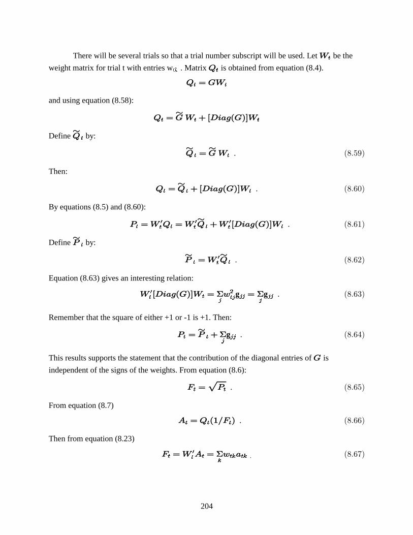
There will be several trials so that a trial number subscript will be used. Let be the��

weight matrix for trial with entries w . Matrix is obtained from equation (8.4).t � ��

� � ��

and using equation (8.58):

� � ��

� � �

Define ��

� by:

� � ��

� � . ��

Then:

� � � � ��

� � � . ��

By equations (8.5) and (8.60):

� ��

� � � �� . ��

Define ��

� by:

� ��

� �� . ��

Equation (8.63) gives an interesting relation:

� ��

� � �g g . ��

Remember that the square of either +1 or -1 is +1. Then:

� � � ��

� � �g . ��

This results supports the statement that the contribution of the diagonal entries of is�

independent of the signs of the weights. From equation (8.6):

� � �� . ��

From equation (8.7)

� � � ��!� �� . ��

Then from equation (8.23)

� ��

�� . ��

205

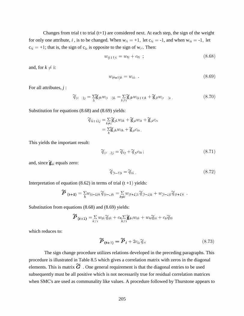
Changes from trial t to trial ( +1) are considered next. At each step, the sign of the weightt

for only one attribute, , is to be changed. When + let c - , and when w - let i w � �i � ��

c + ; that is, the sign of c is opposite to the sign of w . Then:� � ��

" � " � � �� ;

and, for i:k '

" � " �� .

For all attributes, :j

( � " � " � "� � � ��

� ��

�� g g g ��

Substitution for equations (8.68) and (8.69) yields:

( � " � " � ��

� �" � �

��

��

� ��

�

�

g g g

g g�

This yields the important result:

( ( (� � �� ) ��

and, since g�� equals zero:

( (� �� .

Interpretation of equation (8.62) in terms of trial (t +1 yields:�

��

�� " � " � "� �

��

( ( (� � � .

Substitution from equations (8.68) and (8.69) yields:

��

�� " � � " � " � ��

� � � �� ( ( (� � ��g

which reduces to:

� � ��

�� (��

The sign change procedure utilizes relations developed in the preceding paragraphs. This

procedure is illustrated in Table 8.5 which gives a correlation matrix with zeros in the diagonal

elements. This is matrix . One general requirement is that the diagonal entries to be used��

subsequently must be all positive which is not necessarily true for residual correlation matrices

when SMC's are used as communality like values. A procedure followed by Thurstone appears to

206

work very satisfactorily; that is, to use the highest R values for every correlation matrix and

residual correlation matrix. Row D(R) of Table 8.5 contains the highest R (in absolute value) for

the given correlation matrix. The sum of the entries in this row is given at the right. At trial 1, the

weights in row W are all taken to be +1 and the first trial contains the column sums of�

� ��

1�

matrix . Coefficient is the sum of the entries in row . These are the preliminary steps� � ��

1 1 �

before starting the sign change procedure.

Since, by equation (8.64), coefficient is plus the sum of the entries to be inserted� ��

� �

in the diagonal of and this sum is necessarily positive, increasing necessarily increases � � ��

� �

. The objective of the sign change procedure is to increase as much as possible. In each step,��

�

or trial, the attribute is selected whereby is increased most to . By equation (8.73), the� ��

� � ( +1)

change from equals 2c . For this change to be an increase, c and must have� ��

� � to ( +1) � �( (� ��

the same algebraic sign. Note that c is defined to have the opposite sign to w . Therefore, w� � �

and must have opposite signs. The strategy is to select that attribute for which w and (�� (~

have opposite signs and is the largest in absolute value satisfying the signs condition. In the(��

example in Table 8.5, since all weights in row W are positive, the attribute with the most�

�

negative value in row is attribute 3 with an entry of -.84 . Consequently, attribute 3 was��

1�

chosen and a change coefficient c was set at -2 , the sign being opposite to the sign of weight��

w��

After having established rows W , and selected the attribute for the sign change, the�

� *�

1�

next series of steps is to make the changes accompanying this first sign change. In row W the2�

signs of the weights for all attributes except attribute 3 remain unchanged at +1. The weight for

selected attribute 3 is changed to -1 . These weights in row W are the results of application of2�

equations (8.68) and (8.69). Next, row is established as per equations (8.71) and (8.72). For*�

2�

an example consider the first entry in row value of 1.04 equals plus c times* ( (� � �

2� , 21 21. The ��

g��; that is:

1.04 30� � � ��

These computations are continued for all attributes except the selected attribute 3 for which (��

equals a value of -.84 . Coefficient can be computed two ways: one by obtaining the(�� , ��

2

sum of products of entries in rows W and as per equation (8.62); and by equation (8.73).�

� ��

2 ,

For the second method:

3.60 .24 + 2( )( .84)� � �

When using hand computing with the aid of a desk calculator, this value should be computed

both ways to provide a check.

207

A selection is made next of the second attribute to have the sign of its weight changed.

Rows W and are inspected for those attributes having entries with opposite signs and that�

� ��

2�

attribute is selected for which the absolute value of the entry in row is largest. In the��

2�

example, only for attribute 5 are the entries in rows W and opposite in sign; consequently,�

� ��

2�

this attribute is selected to have its sign changed and a -2 is inserted into line c for attribute 5.�

Computations for trial 3 from the results in trial 2 are similar to those carried out in going

from trial 1 to trial 2. The signs of weights in row W are the same as those in row W with3� �

�

exception of w , this being the weight having its sign changed. Entries in row are obtained�5 ��

3�

from row 5 of , the weights in row W , and the entries in row Coefficient is obtained� � ��

�

��

2� . 3

from as well as from the sum of products between entries in rows W and .� ��

2 , c , �5 3(��

25 �

� �

Inspection of rows W and reveals that the signs of the entries in these two rows are�

� ��

3�

in agreement. There are no more signs to be changed. Row W is the final weight vector. A final�

�

row is to be computed by adding in the diagonal entries of with the proper signs, see*� �

equation (8.60). The entry in row of Table 8.5 for the first attribute is:��

1.45 .96 .49 1 � � � ��

For attribute 3:

�� .

For the final coefficient see equation (8.64). The final equals the final plus the sum of� � ��

�

the diagonal entries as well as equaling the sum of the products of the entries in the final and�

�. The value for the example is:

�� .

Factor weights in row are obtained by dividing the entries in row by which equals the�� +

square root of . For the example the factor weight for attribute 1 is:�

�� $�� .

As indicated in equation (8.67), equals the sum of products between the weights in the final�

row of the example and the factor weights in row .� � ��

The example in Table 8.5 is too small to illustrate one kind of difficulty encountered with

larger correlation matrices. Sometimes when the sign has been changed for one attribute and after

a number of further changes the for that attribute becomes positive which is, now, opposite to(�

the sign of the weight. The sign of the weight has to be changed back to a +1 . In this case the

change coefficient, c , is a +2 . Then equations (8.62), (8.71), (8.72), and (8.73) provide the

means for making this reverse change.

208

It is of interest to note now that the use of vectors without the diagonal entries provides��

a more effective sign change than would the use of vectors which includes the diagonal�

entries. For example, in trial 2 of the example in Table 8.5, adding in the diagonal entry of .10 to

(�25 of -.09 yields a value of .01 which agrees in sign with the weight w If this value of .01 is��.

compared with the weight of +1 , then the sign for attribute 5 would not be changed and the

increase in would have been missed.�

We return to the maximization proposition for coefficient . With each trial resulting in�

an increase in , a maximum should be reached since the value can not exceed the sum of�

absolute values of entries in the correlation matrix. However, there is no guarantee that there is

only one maximum nor that an obtained result yields the largest maximum. There is one

statement possible using the vectors without the diagonal entries: it is not possible to increase��

� further after reaching a solution by changing the sign of the weight for only one attribute. To

go from one maximum to another must involve the changing of the weight signs for two or more

attributes. Each solution, thus, involves at least a local maximum. We observe that when a major

maximum has been missed, a solution involving the factor for this maximum is likely to appear

in the results for the next factor extracted from the ensuing residual matrix.

Extraction of centroid factors from the correlation matrix among nine mental tests is

given in Table 8.6 . This correlation matrix was given in Chapter 1, Table 1.1, which includes the

names of tests. For the original correlation matrix given at the top of the first page of this table,

row D(R) contains the highest correlation for each attribute. These values will be substituted for

the unities in the diagonal. Since all correlations are positive, all sign change weights are +1 and

the entries in row are the column sums of the correlation matrix, the diagonal unity having��

been replaced by the entry in row D(R) . Coefficients and are given along with the factor� �

weights in row for the first centroid factor. Coefficient L is a very useful criterion to measureA�

�

the structure indicated in the correlation matrix. In general:

, � � ��

$��

� �g��

This criterion may be used in decisions on the number of factors to be extracted from a

correlation matrix, more about this later. Since all original correlations are positive in the

example, L for this matrix is unity.

The first factor residual matrix is given at the bottom of the first page of Table 8.6. The

diagonal entries are residuals from the substituted diagonals of the correlation matrix. The

column sums including these residual diagonals are zero within rounding error. These sums

provide an excellent check on hand computations. Revised diagonal entries are given in row

D(R) . The signs were changed for attributes 4, 5 , 6, and 8 after which row was obtained��

209

Table 8.6Extraction of Centroid Factors from

Correlation Matrix among Nine Mental Tests

Original Correlation Matrix 1 2 3 4 5 6 7 8 9

1 1.000 2 .499 1.000 3 .394 .436 1.000 4 .097 .007 .292 1.000 5 .126 .023 .307 .621 1.000 6 .085 .083 .328 .510 .623 1.000 7 .284 .467 .291 .044 .114 .086 1.000 8 .152 .235 .309 .319 .376 .337 .393 1.000 9 .232 .307 .364 .213 .276 .271 .431 .489 1.000

D(R)* .499 .499 .436 .621 .623 .623 .467 .489 .489

Q’ 2.368 2.556 3.157 2.724 3.089 2.946 2.577 3.099 3.072

P=25.588 F=5.058 L=1.000

A1’ .468 .505 .624 .539 .611 .582 .509 .613 .607

First Residual Correlation Matrix 1 2 3 4 5 6 7 8 9

1 .290 2 .262 .244 3 .102 .121 .046 4 -.155 -.265 -.044 .331 5 -.160 -.286 -.074 .292 .250 6 -.188 -.211 -.035 .196 .267 .284 7 .046 .210 -.027 -.230 -.197 -.211 .207 8 -.135 -.075 -.073 -.011 .002 -.020 .081 .114 9 -.052 .000 -.015 -.114 -.095 -.083 .122 .117 .120

Sum .000 .000 .001 .000 -.001 -.001 .001 .000 .000

D(R)* .262 .286 .121 .292 .292 .267 .230 .135 .122

Q’ 1.257 1.715 .528 -1.578 -1.665 -1.439 1.137 -.191 .351

P=9.862 F=3.140 L=.859

A2’ .400 .546 .168 -.503 -.530 -.458 .362 -.061 .112

* Hi ghest R.

210

Table 8.6 (Continued)Extraction of Centroid Factors from

Correlation Matrix among Nine Mental Tests

Second Residual Correlation Matrix 1 2 3 4 5 6 7 8 9

1 .102 2 .044 -.013 3 .034 .029 .092 4 .046 .009 .040 .040 5 .052 .004 .015 .026 .011 6 -.004 .039 .042 -.034 .024 .057 7 -.099 .012 -.088 -.048 -.005 -.045 .099 8 -.110 -.041 -.063 -.041 -.030 -.048 .103 .131 9 -.097 -.061 -.034 -.058 -.036 -.032 .081 .124 .109

WeightedSum .000 .000 -.001 -.002 -.001 .001 .000 .001 .000

D(R)* .110 .061 .088 .058 .052 .048 .103 .124 .124

Q’ -.590 -.276 -.433 -.293 -.245 -.238 .561 .685 .645

P=3.967 F=1.992 L=.941

A1’ -.296 -.139 -.217 -.147 -.123 -.120 .281 .344 .324

Third Residual Correlation Matrix 1 2 3 4 5 6 7 8 9

1 .023 2 .003 .042 3 -.030 -.001 .041 4 .003 -.011 .008 .036 5 .016 -.013 -.012 .008 .037 6 -.040 .022 .016 -.052 .010 .033 7 -.016 .051 -.027 -.007 .030 -.011 .024 8 -.009 .006 .012 .009 .012 -.006 .006 .006 9 -.001 -.016 .037 -.010 .004 .007 -.010 .012 .019

WeightedSum -.001 -.001 .000 .000 .000 .001 .000 .000 .000

D(R)* .040 .051 .037 .052 .030 .052 .051 .012 .037

Q’ -.119 .108 .082 -.109 .037 .180 .113 .054 .082

P=.883 F=.940 L=.483

A1’ -.126 .115 .088 -.116 .039 .192 .120 .057 .088

* Hi ghest R.

211

along with coefficients , , and L . For this matrix the sign change did not result in all� �

positive contributions by the off-diagonal entries so that L is less than unity. Factor weights for

the second factor in row A are obtained from row and coefficient .�

� � ��

The second factor residual correlation matrix is given at the top of the second page of

Table 8.6. This matrix is obtained from the first factor residual correlation matrix with

substituted diagonal entries and the second factor weights. The row of weighted sums uses the

just preceding sign change weights as multipliers of the residual correlations. Again, these sums

should equal zero within rounding error which provides a check on hand computations. See

equation (8.22) for the basis for these zero weighted sums. Computation of the third factor

weights progresses in the same manner as the computations for preceding factors.

The third factor residual correlation matrix is given at the bottom of the second page of

Table 8.6. Computations for this matrix and the fourth factor weights are similar to the

computations for preceding factors.

Decisions as to the number of factors to extract by the centroid method had only sketchy

bases to support these decisions. Residual matrices were inspected for the magnitudes of the

entries and factor extraction was stopped when these residuals were small so that they might be

ignored. Table 8.7 gives three coefficients which might be used including the largest residual

correlation in each residual matrix. For the example of nine mental tests the largest third factor

residual was .052 and a decision might be made that this was small enough to be ignored. By this

reason, the three factor solution would be accepted. Another coefficient which might be

considered is the criterion L . Note in the example this coefficient is relatively high for the first

three matrices and factors but drops substantially for the third factor residuals. In this example

the low value of L for the third factor residuals could be taken as an indication to accept the three

factor solution. A third criterion used by some analysts was the magnitude of the factor weights

obtained. Frequently, when the largest factor weight was less than a value such as .2, a factor was

not accepted. In the example this criterion would, again, indicate a three factor solution. Beyond

such criteria as the foregoing, trial transformations of factors was considered and that number of

factors accepted which led to the most meaningful solution. Some individuals advocated using an

extra "residual" factor to help clean up transformed factors.

The centroid method of factor extraction has been presented partly for its historic value

and partly to provide some useful techniques. For example, the sign change technique with

criterion L has been found useful in testing the simplicity of special covariance matrices in

research on the dimensionality of binary data such as item responses. Undoubtedly, there may be

other cases of special covariance matrices for which a simple criterion related to complexity of

the matrix would be helpful.

212

Table 8.7

Illustration of Indices used for Number of Factors

in Centroid Factor Extraction

LargestCorrelation

CriterionL

LargestFactor Loading*

Original Correlation matrix, Factor 1 .623 1.000 .624First Residual Matrix, Factor 2 .292 .859 .546Second Residual Matrix, Factor 3 .124 .941 .344Third residual Matrix, Factor 4 .052 .483 .192

* In absolute value

213

8.4. Group Centroid Method of Factor Extraction

The group centroid method of factor extraction provides a simple technique which may

be applied in special situations. In particular, a partitioning of the attributes into clusters with

high within cluster correlations should be possible. The correlations between clusters should be

low. For an example consider the correlation matrix in Table 8.8. Attributes 1, 2, and 4

intercorrelate relatively highly and have low correlations with the remaining attributes. These

attributes are listed first in Table 8.9. Ignore the diagonal entries for the present. Attributes 5 and

6 have a high correlation while attribute 3 correlates negatively with them. A sign reversal of the

correlations of attribute 3 produces moderately high, positive correlations with attributes 5 and 6.

In making such a sign reversal, the signs of the correlations in both the rows and the columns are

reversed for the attribute. Note that the diagonal entry remains positive since its sign is reversed

twice. This operation yields the second cluster in Table 8.9. As seen in this table, there are two

clusters of attributes with relatively high intercorrelations within the clusters and relatively low

correlations between clusters. This is the type of situation for which the group centroid method of

factor extraction could be appropriate.

For the operation of the group centroid method of factor extraction return to the original

correlation matrix in Table 8.8; the clustered correlation matrix provided a guiding step but will

not be used in the computations. A first consideration is the diagonal entries. The extracted

factors will depend on the intercorrelations of the attributes in the clusters, these intercorrelations

forming relatively small matrices. There is a problem in using SMC's as diagonal entries. As

shown earlier, the SMC's tend to be smaller than desired for small matrices. For example, the

SMC for attribute 1 in our example is .274 which appears small for the intercorrelations of the

attributes in the example. In contrast, the "highest R" of .44 appears appropriate. Further, for

computations using a desk calculator, the "highest R" technique is much more convenient. Thus,

in general with the group centroid method of factor extraction, the "highest R" would be the

preferred value to be inserted into the diagonal of the correlation matrix. This has been done for

the middle matrix of Table 8.8 and were given in Table 8.9. Computations of the factor matrix

will progress from the middle matrix of Table 8.8.

Equations used in the group centroid method of factor analysis method are repeated here

for convenience. Matrix is the correlation matrix with desired diagonal entries such as the��

middle matrix of Table 8.8.

� � � �� . ��

� �� . ��

214

Table 8.8

Correlation matrices for

Illustration of Group Centroid Method of Factor Extraction

Correlation Matrix with Unities in Diagonal

1 2 3 4 5 61 1.00 .44 -.04 .43 .04 .052 .44 1.00 -.06 .38 .07 .093 -.04 -.06 1.00 -.06 -.33 -.354 .43 .38 -.06 1.00 .09 .085 .04 .07 -.33 .09 1.00 .406 .05 .09 -.35 .08 .40 1.00

Correlation Matrix with Highest R’s in Diagonal

1 2 3 4 5 61 .44 .44 -.04 .43 .04 .052 .44 .44 -.06 .38 .07 .093 -.04 -.06 .35 -.06 -.33 -.354 .43 .38 -.06 .43 .09 .085 .04 .07 -.33 .09 .40 .406 .05 .09 -.35 .08 .40 .40

Residual Correlation Matrix

1 2 3 4 5 61 -.01 .01 -.01 .01 -.01 .002 .01 .02 .00 -.03 -.01 .013 -.01 .00 .03 .01 .02 .014 .01 -.03 .01 .03 .01 -.015 -.01 -.01 .02 .01 .01 .016 .00 .01 .01 -.01 .01 .00

215

Table 8.9

Clustered Correlation Matrix for

Illustration of Group Centroid Method of Factor Extraction

Correlation Matrix with Highest R’s in Diagonal

1 2 4 5 6 -31 .44 .44 .43 .04 .05 .042 .44 .44 .38 .07 .09 .064 .43 .38 .43 .09 .08 .06

5 .04 .07 .09 .40 .40 .336 .05 .09 .08 .40 .40 .35-3 .04 .06 .06 .33 .35 .35

216

�� . ��

� � �� . ��

� � � ��

where is the matrix of residual correlations.��

� �� . ��

Reference will be made to these equations during the discussion of the computing procedures.

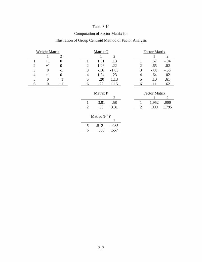
Computations for the example are given in Table 8.10. Weight matrix is the starting�

point. This matrix reflects the clusters which have been determined during inspection of the

correlation matrix. There is a column of for each cluster, or group, and contains weights of�

+1 or -1 for attributes in the cluster and weights of 0 for attributes not in the cluster. Weights of

+1 are assigned to attributes which are not reflected in sign and weights of -1 for attributes

reflected in sign. In the example, the first cluster was composed of attributes 1, 2, and 4 without

any reflections in sign. Consequently, the first column of weight matrix in Table 8.10 has +1's

for these three attributes and 0's for the other attributes. The second column of the weight matrix

is for the second cluster with +1's for attributes 5 and 6 and a -1 for attribute 3 since this attribute

was reflected in sign to form the cluster. The weight of -1 performs this reflection. In this second

column of weights, 0's are recorded for attributes 1, 2 , and 4 which are not in the second cluster.

In general, the weight matrix reflects the clusters found during inspection of the correlation

matrix.

Once the weight matrix has been established, computations follow the given equations.

Matrix is computed by equation (8.4). Since the weight matrix contains only +1's , -l's , and�

0's, this matrix multiplication involves only addition, or subtraction, of entries in the correlation

matrix and may be accomplished quite readily with a desk calculator. Matrix is obtained by�

equation (8.5) which, again, involves only addition or subtraction of entries in . Matrix is a� �

decomposition of as indicated by equation (8.6). A Cholesky decomposition of to triangular� �

matrix is most convenient. At this point note a requirement that matrix must be of full rank.� �

This reflects on the composition of the weight matrix and the correlation matrix. Having matrix

� � its inverse is obtained, this being a simple solution when is triangular. The matrix of factor

weights is obtained by equation (8.7). Equation (8.23) gives an interesting relation.

Once the factor matrix has been determined, a matrix of residual correlations should be

computed by equation (8.8). For the example, the matrix of residual correlations is given at the

bottom of Table 8.8. For our example, these residuals are all quite tiny indicating that the

217

Table 8.10

Computation of Factor Matrix for

Illustration of Group Centroid Method of Factor Analysis

Weight Matrix Matrix Q Factor Matrix 1 2 1 2 1 2

1 +1 0 1 1.31 .13 1 .67 -.042 +1 0 2 1.26 .22 2 .65 .023 0 -1 3 -.16 -1.03 3 -.08 -.564 +1 0 4 1.24 .23 4 .64 .025 0 +1 5 .20 1.13 5 .10 .616 0 +1 6 .22 1.15 6 .11 .62

Matrix P Factor Matrix 1 2 1 2

1 3.81 .58 1 1.952 .0002 .58 3.31 2 .000 1.795

Matrix (F-1)’ 1 2

5 .512 -.0856 .000 .557

218

obtained factor matrix provides an excellent fit to the input correlation matrix. When the fit is not

as good, further factors could be extracted from the residual matrix and added to the factor

matrix by adjoining these new factors to those already obtained. New attribute clusters could be

determined in the residual matrix and the group centroid method used to establish these new

factors. An alternative is to apply the centroid method to the matrix of residual correlations.

The group centroid method of factor extraction appears to be a simple technique which

could be useful in less formal analyses such as for pilot studies and analyses. For more formal

studies more precise methods would be advisable.

8.5. Principal Factors Method of Factor Extraction

With the development of digital computers the principal factors method has become the

most popular method for factor extraction. Prior to the large computer the calculation labor was

prohibitively extensive to use this method on any but the most trivial sized matrices. The key to

use of principal factors is the availability of solutions for eigenvalues and eigenvectors of real,

symmetric matrices. Now, these solutions may be obtained quite readily for all but very large

correlation and covariance matrices. The principal factors method has a number of desirable

properties including a maximization of the sum of squares of factor weights on the extracted

factors. Minimization of the sum of squares of residual correlations will be discussed in detail in

the next chapter.

A numerical example is discussed before a presentation of mathematical properties of

principal factors. Table 8.11 gives the correlation matrix for the nine mental tests example with

SMC's in the diagonal. The eigenvalues and eigenvectors were computed for this matrix and are

presented in Table 8.12. Note that all eigenvalues after the first three are negative. Use of SMC's

in the diagonal of a correlation matrix must result in a number of negative eigenvalues. At the

bottom of Table 8.12 is the principal factors matrix, each column of which being obtained by

multiplying the entries in an eigenvector by the square root of corresponding eigenvalue. There

are only three columns in the principal factors matrix since the square roots of the eigenvalues

beyond the first three present problems with imaginary numbers. However, in some studies, the

factor extraction may stop short of number of positive eigenvalues, this being a problem as to

the number of factors which will be discussed subsequently.

Mathematical relations for principal factors are considered next. Let be a square,�

symmetric matrix with real numbers. There is no restriction that be Gramian as was stated in�

the general theory of matrix factoring; however, a number of the relations given in the general

theory will be used. There must be considerable care in this usage to avoid violating several

restrictions. For example, matrix could be a correlation matrix with SMC's in the diagonal�

such as given for the nine mental tests in Table 8.11. As seen in Table 8.12, there are a number of

219

Table 8.11

Correlation and Residual Matrices for

Principal Factors for Nine Mental tests

Correlation Matrix with SMC’s in Diagonal

1 2 3 4 5 6 7 8 91 .297 .499 .394 .097 .126 .085 .284 .152 .2322 .499 .424 .436 .007 .023 .083 .467 .235 .3073 .394 .436 .356 .292 .307 .328 .291 .309 .3644 .097 .007 .292 .428 .621 .510 .044 .319 .2135 .126 .023 .307 .621 .535 .623 .114 .376 .2766 .085 .083 .328 .510 .623 .440 .086 .337 .2717 .284 .467 .291 .044 .114 .086 .350 .393 .4318 .152 .235 .309 .319 .376 .337 .393 .361 .4899 .232 .307 .364 .213 .276 .271 .431 .489 .349

First Residual Correlation Matrix

1 2 3 4 5 6 7 8 91 .123 .303 .140 -.128 -.137 -.159 .083 -.101 -.0142 .303 .204 .150 -.247 -.273 -.191 .241 -.050 .0303 .140 .150 -.014 -.037 -.078 -.028 -.002 -.060 .0054 -.128 -.247 -.037 .136 .280 .194 -.216 -.009 -.1065 -.137 -.273 -.078 .280 .136 .254 -.190 -.007 -.0976 -.159 -.191 -.028 .194 .254 .098 -.196 -.018 -.0747 .083 .241 -.002 -.216 -.190 -.196 .118 .101 .1478 -.101 -.050 -.060 -.009 -.007 -.018 .101 -.007 .1319 -.014 .030 .005 -.106 -.097 -.074 .147 .131 .001

Second Residual Correlation Matrix

1 2 3 4 5 6 7 8 91 -.009 .108 .083 .037 .038 -.011 -.064 -.102 -.0722 .108 -.085 .066 -.001 -.014 .028 .024 -.051 -.0553 .083 .066 -.039 .035 -.002 .036 -.066 -.061 -.0204 .037 -.001 .035 -.071 .060 .008 -.032 -.008 -.0345 .038 -.014 -.002 .060 -.096 .057 .004 -.006 -.0206 -.011 .028 .036 .008 .057 -.069 -.031 -.017 -.0107 -.064 .024 -.066 -.032 .004 -.031 -.045 .100 .0838 -.102 -.051 -.061 -.008 -.006 -.017 .100 -.007 .1319 -.072 -.055 -.020 -.034 -.020 -.010 .083 .131 -.024

220

Table 8.11(Continued)

Third Residual Correlation Matrix

1 2 3 4 5 6 7 8 91 -.086 .064 .029 .012 .023 -.028 -.006 -.020 -.0022 .064 -.110 .035 -.015 -.022 .019 .056 -.005 -.0163 .029 .035 -.077 .017 -.012 .024 -.025 -.004 .0294 .012 -.015 .017 -.079 .056 .002 -.013 .019 -.0115 .023 -.022 -.012 .056 -.098 .054 .015 .009 -.0076 -.028 .019 .024 .002 .054 -.073 -.018 .001 .0067 -.006 .056 -.025 -.013 .015 -.018 -.088 .039 .0318 -.020 -.005 -.004 .019 .009 .001 .039 -.093 .0579 -.002 -.016 .029 -.011 -.007 .006 .031 .057 -.087

221

Table 8.12

Computation of Principal Factors Matrix for Nine Mental Tests Example from

Correlation Matrix with SMC’s in Diagonal

Eigenvalues

1 2 3 4 5 6 7 8 92.746 1.241 .346 -.048 -.064 -.125 -.153 -.175 -.255

Eigenvectors

1 2 3 4 5 6 7 8 91 .252 .326 .472 .265 -.213 .511 .259 .052 .4012 .283 .483 .266 .094 .305 -.267 .190 .228 -.5953 .367 .141 .331 -.557 -.258 -.279 -.272 -.447 .0844 .326 -.409 .154 .311 -.444 -.437 -.082 .456 .0575 .381 -.433 .087 .349 .146 .349 -.213 -.440 -.3946 .353 -.366 .106 -.355 .629 .035 .178 .263 .3267 .291 .362 -.353 .393 .292 -.214 -.448 -.084 .4078 .366 .002 -.499 .019 -.184 -.146 .684 -.305 .0309 .356 .14 -.425 -.334 -.249 .456 -.265 .418 -.214

Principal Factor Matrix

1 2 31 .417 .363 .2782 .469 .538 .1563 .609 .157 .1954 .540 -.456 .0905 .632 -.482 .0516 .585 -.408 .0627 .481 .404 -.2088 .607 .003 -.2939 .590 .159 -.250

222

negative eigenvalues for this matrix so that this matrix is not Gramian. Further, residual

correlation matrices must have as many eigenvalues equal to zero as the number of factors that

have been extracted. Allowance must be made for zero and negative eigenvalues in the

development.

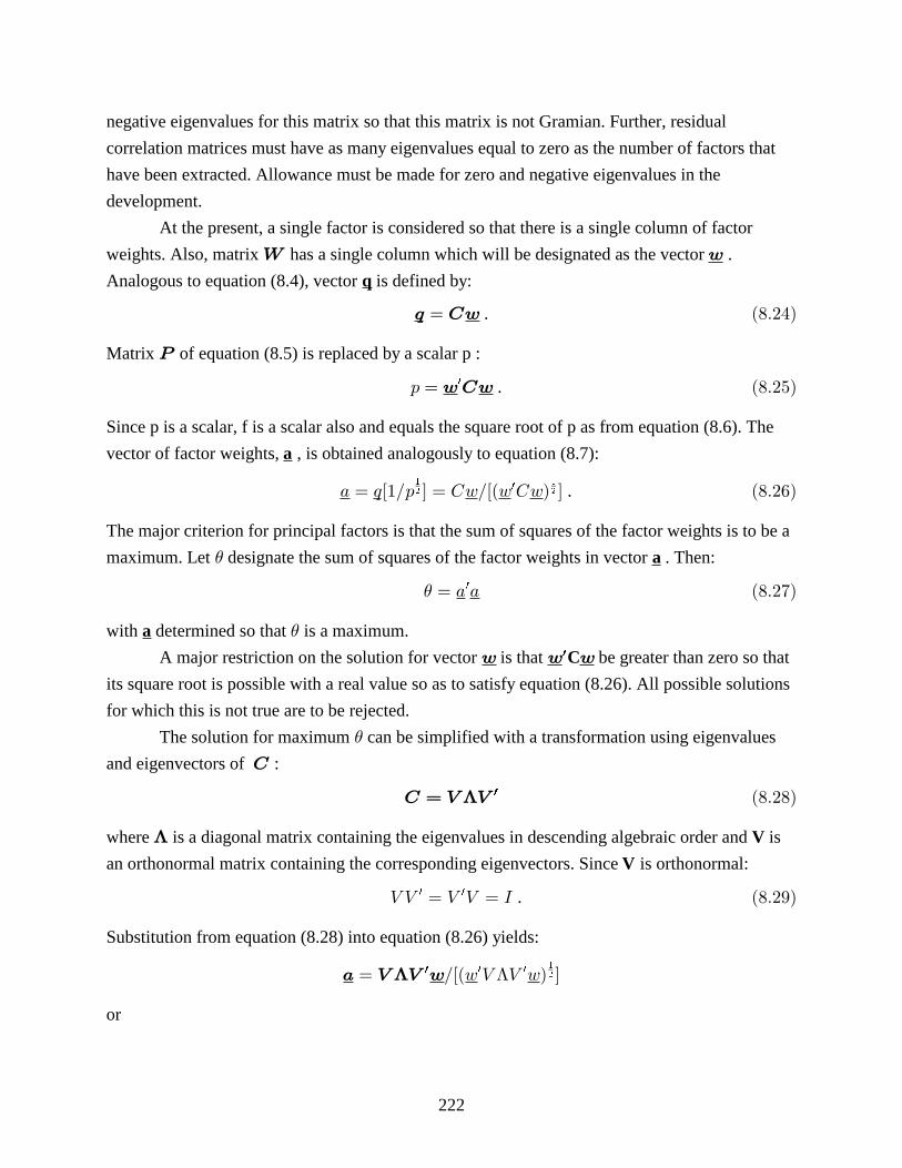
At the present, a single factor is considered so that there is a single column of factor

weights. Also, matrix has a single column which will be designated as the vector .�

Analogous to equation (8.4), vector is defined by:q

" � � . ��

Matrix of equation (8.5) is replaced by a scalar p :�

- � �� .

Since p is a scalar, f is a scalar also and equals the square root of p as from equation (8.6). The

vector of factor weights, , is obtained analogously to equation (8.7):a

� � ��$- � � . $�� . � � ��( " "� �

� �" � .

The major criterion for principal factors is that the sum of squares of the factor weights is to be a

maximum. Let designate the sum of squares of the factor weights in vector . Then:� a

� � ��

with determined so that is a maximum.a �

A major restriction on the solution for vector is that be greater than zero so that �C

its square root is possible with a real value so as to satisfy equation (8.26). All possible solutions

for which this is not true are to be rejected.

The solution for maximum can be simplified with a transformation using eigenvalues�

and eigenvectors of :�

� � # #� � ��

where is a diagonal matrix containing the eigenvalues in descending algebraic order and is� V

an orthonormal matrix containing the corresponding eigenvectors. Since is orthonormal:V

/ / � / / � 0 �� .

Substitution from equation (8.28) into equation (8.26) yields:

� $�� / / � �# #� � " "� ��

�

or

223

/ � / $�� / / � � �� " " "� ��

� .

Define vectors and by: � �

� � # � ; ��

� � # � . ��

Then:

� � � �� $��

�

� , ��

and from equation (8.27)

� � �� # # �� .

With equation (8.33)

� � �� !� �� .

To obtain a maximum a partial derivative with respect to the elements of vector is set equal� �

to zero. There may be several optima with the largest solution being chosen.

1

1� � � ��

�

�� !� � � ��

� � �� .

With the restriction that be finite and not equal to zero:� ��

� � � �� !� �� . ��

Using equation (8.35) with algebraic manipulations yields:

� ��

which is the equation for an eigen problem with eigenvalues and eigenvectors ( ) . Note that� � �

( ) is a vector with entries ( for 1, 2 n .� � � �" �� 2 � �3 �

Since is a diagonal matrix, the eigenvalues of equation (8.38) equal the diagonal� �

values of . Also, since the eigenvalues of are in descending algebraic order, the maximum� � �

� equals the first . Thus:�

�� . �$%&'�

The first eigenvector has an entry of unity for the first element and entries of zero for remaining

entries.

� ��" � � ��

224

� 2 � �4� 5 ��" � � �� for .

From (8.40)

" � �$��

so that

� � � �!� � ��

Unless all eigenvalues of are zero or negative, the obtained solution is acceptable.�

The first factor weights are considered next. A subscript 1 is used with vectors , � � ,

and to designate this first factor. From equations (8.33) and (8.43):

� � � � �� " " �� $��$ ��

�

�

�

� .


� � � �� # � # � ��

�

�

From equations (8.40) and (8.41) vector has a first entry of unity with all other entries��

equal to zero. Let matrix be partitioned as below:#

# � �# # ��

where is 1 containing the first column of and is ( -1) containing the# # #� �n n n� �

remaining columns of . With this construction and nature of vector ( ) :# ��

� � �� # �$%()��

�

which is the equation for the first factor weights.

The preceding paragraph concerned the first principal factor. Each of the eigenvalues �

greater than zero yields a principal factor. The sum of squares of the factor loadings on each of

these factors is :��

�� $%(*�

The 'th element of the eigenvector ( ) equals unity while the remaining elements equal zero.j � �

Following similar steps which led to equation (8.45), the vector of factor weights is:

� # �$%(+��

� .

As will be presented subsequently, each of these principal factors will be the first principal factor

for a matrix of residual covariances.

225

The preceding results may be combined to yield a factor matrix for r principal factors. Let

�� be a factor matrix for the first r principal factors. Also, let be an matrix containing#� n r�

the first r eigenvectors and be an diagonal matrix containing the first r eigenvalues of�� r r�

� . Then, equations (8.45) and (8.47) may be combined to:

�� # ��

� . ��

Since is a vertical section of an orthonormal matrix:#�

# # � ��

�� .

Then:

� � ��

�� . �$%('�

The columns of are orthogonal and their sums of squares equal the corresponding eigenvalues�r

of . For the nine mental tests example, three principal factors were extracted; thus, r = 3 . The�

principal factors matrix is given at the bottom of Table 8.12. Multipliers for the three columns of

eigenvectors are the square roots of the first three eigenvalues, these square roots being: 1.657,

1.114, and .588. The three columns of principal factors matrix are obtained by multiplying the

corresponding columns of eigenvectors by these multipliers.

Residual correlation matrices are considered next. When one principal factor is extracted

at a time there is a sequence of residual matrices with one factor being obtained from one such

matrix and a residual matrix being determined from the matrix used in determining the factor.

For the nine mental tests example, this series of residual correlation matrices is given in Table

8.11. The operations will be similar for each of these steps so that only the first factor residual

matrix will be considered explicitly. Let designate the first factor residual matrix. From�•�

equation (8.8):

� � � �•� � �

� . ��

Equations are written in this section with expanded matrices involving partitions of 1 factor and

( -1) factors similar to the expansion used previously for matrix . The eigenvalues andn #

eigenvectors of written as:� in equation (8.28) are

� ��

� �� # �#

� ##� �

�

�

�

�

�

�

�

��

where matrix in the present context, is an ( -1) ( -1) diagonal matrix containing the�� , n n�

eigenvalues after the first one. The matrix product is expressed as: � �

�

226

� �

��

�

�� .

with:

� � � � � �# # � �� ,

0� ��

� ��

� � ��

� � �

�

�

�� # � # �� #

#� �� 0

��

In the subtraction of from , as per equation (8.50), the eigenvectors on the left and right � �

� �

are factored out so that:

� � ��

��•� # �# �� #

#� �

�

�

�

�

��

��

Thus, the first eigenvalue of has been replaced by a zero for so that the largest eigenvalue� �•�

of is the second largest eigenvalue of . Note that the eigenvectors have not been changed.� �•�

As a consequence of the foregoing, the first principal factor of is the second principal factor�•�

of . In a similar manner going from the first factor residual matrix to the second factor residual�

matrix sets the second eigenvalue of to zero and the third principal factor of is the first� �

principal factor of the second residual matrix. These relations continue through as many factors

as are extracted.

Several types of information are used in judging the number of factors to be extracted.

However, not one criterion can be trusted completely so that an analyst must consider several

indications available before making a judgment as to the number of factors. This is in contrast to

a common procedure in computer packages which use a single criterion to automate this

judgment so that each analysis can be completed automatically in a single run. Several of the

types of information for number of factors will be discussed in following paragraphs.

An important point is that factor extraction is only the first part of a complete analysis.

After an original factor matrix has been established, there is factor transformation. The

transformed factors do not correspond directly, one to one, to the extracted factors but are

mixtures of the extracted factors. A final criterion for number of factors extracted is the validity

and interpretability of the transformed factor structure.

Major indicators for the number of factors are derived from the series of eigenvalues of

the correlation matrix with unities in the diagonal cells and with SMC's in the diagonal cells. A

procedure, called by some individuals as "root staring", involves inspection of the series of

227

eigenvalues, especially of the correlation matrix with SMC's in the diagonal cells. Table 8.13

lists the eigenvalues of the correlation matrix with unities in the diagonal cells and with SMC's in

the diagonal cells for the nine mental tests example. Figure 8.1 presents a graph of the

eigenvalues of the correlation matrix with SMC's in the diagonal. In this graph, the eigenvalues

are plotted against the number of the eigenvalue. This graph illustrates results frequently

obtained for well edited test batteries, the series of eigenvalues after a few large ones form an

almost straight line. This phenomena may be interpreted as indicating that there are two

influences in the formation of the data: first, a relevant factor structure and a second influence of

random noise. Cattell (1966) described his "Scree Test" for the number of common factors based

on the foregoing observation. The points in an eigenvalue graph are not to be interpreted as

goodness of fit measures. If they were so interpreted, factor extraction would continue until a

satisfactory goodness of fit is obtained. In contrast, factor extraction should be continued as long

as eigenvalues are above the random noise line. Thus, for the nine mental tests example a three

factor solution would be accepted. However, Thurstone as well as Cattell advocated extracting

one or more extra factors which might be used in the factor transformation process to "clean up"

the meaningful transformed factors. Such an operation should be followed only with great care.

An alternative to making an eigenvalue graph is illustrated in Table 8.13. On the right of

the section for the eigenvalues of the correlation matrix with SMC's in the diagonal is a column

of differences. These values are the differences between consecutive eigenvalues. Geometrically,

for a straight line of points, such differences would be equal. Since the eigenvalues are ordered in

descending algebraic value, all of the differences between consecutive eigenvalues must be equal

to or greater than zero. Then, a series of points which approximate a straight line would have

almost equal, positive differences. For the nine mental tests series of differences in Table 8.13,

starting with the difference between the fourth and fifth eigenvalue, the values of the differences

are quite small with little variation when compared with preceding differences. The last large

difference is between the third and fourth eigenvalue indicating that the third eigenvalue is the

last one above the random noise line.

Guttman (1964) developed three lower bounds for the number of common factors for a

correlation matrix. In this development he considered only cases for population correlation

matrices for which the common factor model fitted exactly. Guttman's strongest lower bound for

the number of common factors is the number of non-negative eigenvalues of the correlation

matrix with SMC's in the diagonal cells. That is, the number of common factors is equal to or

greater than the number of these eigenvalues which are positive, including those equal to zero.

As can be seen from Table 8.13 for the nine mental tests example, by this criterion there are at

least 3 common factors for this matrix. However, as shown by Kaiser and Hunka (1973) from

analyses of 64 correlation matrices found in the literature, this criterion leads to the extraction of

228

Table 8.13

Information for Number of Factors from

Eigenvalues of Correlation Matrix for Nine Mental Tests Example

Correlation Matrix with

Unities in Diagonal SMC’s in Diagonal Eigenvalues Eigenvalues Differences

1 3.347 1 2.7461.505

2 1.820 2 1.241.894

3 .997 3 .346.395

4 .580 4 -.048.016

5 .549 5 -.064.061

6 .497 6 -.125.028

7 .476 7 -.153.022

8 .412 8 -.175.050

9 .322 9 -.225

Parallel Analysis for Eigenvalues

Real DataApproximateRandom Data Differences

1 2.746 .189 2.5572 1.241 .127 1.1143 .346 .087 .2594 -.048 .049 -.097

229

Eigenvalue Number

0 2 4 6 8 10

Eig

enva

lue

-1.0

0.0

1.0

2.0

3.0

Figure 8.1: Eigenvalue graph for correlation matrix with SMC's in the diagonal, nine mental tests example

230

a large number of factors. They conclude that this "lower bound is not of practical use in

determining the effective number of common factors." An illustration of this stronger lower

bound leading to an undesirably large number of extracted factors is given in a second example

presented subsequently.

Guttman's weaker lower bound for the number of common factors is the number of

eigenvalues of the correlation matrix with unities in the diagonal cells equal to or greater than

one. This is a very commonly used value in computer packages for the number of factors to be

extracted. Following considerable experience in analyzing a variety of correlation matrices,

Kaiser (1960) suggested a simple, approximate procedure using principal components analysis

and extracting the number of components equal to Guttman's weaker lower bound. Later, this

procedure became called "Little Jiffy" after a remark by Chester Harris. Use of this weaker lower

bound has been carried over to computer packages. Analysts, however, must remember that this

is a and may lead to extracting too few factors. See the first column of values inlower bound

Table 8.13 for the nine mental tests example, these are the eigenvalues of the correlation matrix

with unities in the diagonal cells. There are two eigenvalues greater than 1.000 so that Guttman's

weaker lower bound for the number of factors would indicate that there are at least two common

factors. The third eigenvalue is just less than 1.000; however, a computer output from a number

of computer packages would extract only two factors.

Table 8.14 presents results from transformations of the two factor solution and the three

factor solution for the nine mental tests example. The two factor solution was indicated by a

blind following of the procedure based on Guttman's weaker lower bound. The three factor

solution was indicated by the series of eigenvalues of the correlation matrix with SMC's in the

diagonal. These results illustrate the types of difficulties which may be encountered when too few

factors are extracted. For the three factor solution the three transformed factors are the previously

identified numerical operations factor, the spatial factor, and the perceptual speed factor. For the

two factor solution, the perceptual speed factor has been collapsed into the numerical operations

factor. The spatial factor representation in the two factor solution was OK. Limiting the common

factor space by extracting too few factors causes a loss of some weaker factors with the attributes

then having improper weights on other factors. As a result, the transformed factor solution is

defective. As Kaiser has put it (personal communication) "it's a sin to extract too few factors."

Remember that eigenvalues (roots) greater than one of the correlation matrix with unities in the

diagonal is a to the number of factors. Analysts should inspect computer outputs tolower bound

see if too few factors were extracted. If more factors are indicated, a computer parameter should

be set for a rerun to use a larger number of factors.

Humphreys with Ilgen and Montanelli (see Humphreys and Ilgen (1959), Humphreys and

Montanelli (1975), Montanelli and Humphreys (1976)) developed a different type of information

231

Table 8.14Transformed Factor Weight Matrices from

Principal Factors for Nine Mental Tests Example

Factor Weights

Two Factor Solution Three Factor Solution Test 1 2 1 2 3Addition 1 .55 .02 1 .66 .05 -.09Multiplication 2 .72 -.07 2 .67 -.05 .11Three-Higher 3 .50 .31 3 .52 .32 .01Figures 4 -.03 .71 4 .00 .72 -.04Cards 5 .00 .79 5 -.02 .80 .03Flags 6 .03 .71 6 .02 .71 .02Identical Numbers 7 .62 .04 7 .24 .03 .49Faces 8 .38 .42 8 -.06 .40 .53Mirror Reading 9 .49 .30 9 .08 .28 .52

Factor Intercorrelations

Two Factor Solution Three Factor Solution 1 2 1 2 3

1 1.00 .16 1 1.00 .15 .572 .16 1.00 2 .15 1.00 .11

3 .57 .11 1.00

232

relevant to the number of factors to be extracted. Their suggestion was to compare results

obtained from the real data with results obtained from random data. Paralleling the real data

score matrix, they drew a matrix of random normal deviates (mean = 0, SD = 1) having the same

number of rows and columns as the real data matrix. They, then obtained a correlation matrix for

the random data and found the eigenvalues of this matrix with SMC's in the diagonal. Their idea

was to continue factor extraction until the eigenvalues for the real data were not larger than the

eigenvalues for the random data. See the bottom section of Table 8.13 for an example. The first

column for "Real Data" is a copy of the first four eigenvalues given above for the correlation

matrix having SMC's in the diagonal. The middle column for "Approximate Random Data" was

computed by a procedure to be given later. The third column gives the differences between the

real data eigenvalues and the approximate random data eigenvalues. Note that the first three real

data eigenvalues are materially greater than the approximate random data eigenvalues while there

is a switch at the fourth pair of eigenvalues. The parallel analysis criterion indicates that three

factors should be extracted from this correlation matrix. In general, Humphreys and associates

suggest that when the real data eigenvalues are not greater than the random data eigenvalues the

real data eigenvectors and factors contain no more real information than exists for the random

data. Consequently, factor extraction can be stopped.

To implement the parallel analysis procedure Montanelli and Humphreys (1976) ran a

large Monte Carlo study involving replications of random data analyses for a selection of matrix

sizes. The numbers of statistical individuals were 25 , 96 , 384 . or 1533 . They used a total of 21

battery sizes ranging from 6 to 90 . The number of replications per cell varied from 10 to 40 with

the cells having fewer replications being those for the larger sample sizes. For each matrix order,

N , a series of mean eigenvalues across replications was computed, each of these mean� n

values being for the 'th eigenvalue. Montanelli and Humphreys provided a system to2

approximate such series of eigenvalues using tabled weights. The data of means was provided to

Tucker who developed a system for use with a computer to approximate the mean eigenvalues. A

first point is that the eigenvalues for random data become negative after eigenvalues wherem

m= n n n�

�5 for even and ( - 1) for odd. As a consequence, the series of eigenvalues is truncated�

�

after the 'th eigenvalue. Following are the equations for Tucker's system.�

5 � 5�6 � ��$6 ��

7 � 8596 � � � ��6 � �5�$6�6 � �5�: ��

7 � 859 5 �5 � �� 52 � ��5$9� � �85� �2$5�� :: ��

��

� � �

233

� � �� 85�2 � � �� •

; � �� 85�2 � �� •

; � �� 85�2 � �� •

where N is the sample size, is the battery size, and is the eigenvalue number. Then, then i

approximation to the random data eigenvalue is :�<��

�< � =7-�� ; 7 � ; 7 � ��

The approximate random data eigenvalues in Table 8.13 were computed by this system. Tucker

used an empirical, trial and error procedure. Measures of goodness of fit to the Montanelli and

Humphreys data indicated a satisfactory level for practical use.

A second example of principal factor extraction is presented in Tables 8.15 through 8.17

and Figure 8.2. This example uses 18 verbal and numerical tests selected from a 66 test battery

by Thurstone and Thurstone (1941). Table 8.15 gives the correlation matrix with the test names

being given in Table 8.17. First consideration is given to the number of factors to be extracted.

For the roots greater than one from the correlation matrix with unities in the diagonal, the fourth

eigenvalue is 1.122 while the fifth eigenvalue is .741. By this criterion there are four common

factors. Figure 8.2 presents the eigenvalue plot for the correlation matrix with SMC's in the

diagonal. There are four eigenvalues above a well defined line for random noise eigenvalues. By

this criterion there appear to be four common factors to be extracted. The parallel analysis is

given in Table 8.16. The first four real data eigenvalues are distinctly greater than the

corresponding approximate random data eigenvalues while there is a switch at eigenvalue 5 for

which the real data eigenvalue is less than the approximate random data eigenvalue. By this

criterion, also, there appears to be four common factors. From the convergence of these three

criteria for the number of factors to be extracted, a decision to consider a four factor solution is

well justified.

A second look at the Guttman stronger lower bound for the number of factors is provided

in Table 8.16. The first 9 real data eigenvalues are listed for the correlation matrix with SMC's in

the diagonal. Guttman's stronger lower bound states that there are at least as many common

factors as the number of these eigenvalues that are non-negative. For the 18 verbal and numerical

test example, this criterion indicates that there are at least 8 common factors. This is an

undesirable answer when compared with the number of factors indicated by the criteria discussed

in the preceding paragraph. The Kaiser and Hunka (1973) conclusion appears to be upheld that

the Guttman stronger lower bound is not usable for real world data. Table 8.17 contains the

principal factors matrix for the 18 verbal and numerical tests example.

234

Table 8.15

Correlation Matrix among 18 Verbal and Numerical Tests Example

1 2 3 4 5 6 7 8 91 1.000 2 .264 1.000 3 .232 .231 l.000 4 .276 .465 .311 1.000 5 .221 .248 .378 .460 1.000 6 .284 .034 .431 .221 .237 1.000 7 .234 .243 .377 .367 .357 .286 1.000 8 .207 .395 .378 .439 .400 .154 .437 1.000 9 .499 .208 .307 .328 .281 .467 .295 .203 1.000 10 .160 .092 .294 .236 .254 .299 .294 .321 .24211 .195 .444 .220 .476 .384 .054 .237 .308 .18312 .126 .403 .307 .420 .349 .116 .341 .473 .12613 .159 .430 .209 .497 .454 -.008 .226 .335 .13314 .184 .420 .206 .511 .455 .026 .l87 .342 .17215 .168 .365 .240 .486 .497 .126 .258 .326 .21016 .165 .329 .331 .342 .256 .238 .396 .473 .16317 .394 .454 .364 .411 .341 .291 .334 .376 .43618 .217 .230 .385 .490 .541 .407 .291 .303 .356

10 11 12 13 14 15 16 17 1812345678910 l.000 11 .112 1.000 12 .218 .385 l.000 13 .048 .624 .396 1.000 14 .090 .623 .4l8 .769 1.000 15 .112 .550 .396 .730 .661 1.000 16 .296 .239 .459 .212 .241 .223 1.000 17 .274 .324 .313 .281 .331 .310 .330 1.000 18 .224 .418 .387 .439 .479 .500 .277 .364 1.000

* Selected from 66 test study by Thurstone and Thurstone (1941), Factorial studies ofintelligence; samole size=710.

235

Table 8.16

Eigenvalues and Parallel Analysis for 18 Verbal and Numerical Tests Example

Real DataApproximateRandom Data Differences

1 6.031 .316 5.7152 1.649 .254 1.3953 .764 .209 .5544 .532 .175 .3575 .112 .146 -.0356 .054 .120 -.0667 .020 .094 -.0748 .011 .065 -.0549 -.013 .017 -.030

236

Table 8.17

Principal Factors Matrix for 18 Verbal and Numerical Tests Example

Test 1 2 3 4Addition 1 .39 .28 .22 .31Arithemetic (Word Problems) 2 .57 -.12 -.17 .36Mirror Reading 3 .52 .33 -.03 -.14Directions 4 .71 -.04 -.01 .06Disarranged Sentences 5 .65 .01 .09 -.22Identical Numbers 6 .35 .53 .24 -.16Letter Grouping 7 .52 .27 -.18 -.06Letter Series 8 .61 .12 -.36 .00Multiplication 9 .45 .41 .34 .19Number Patterns 10 .34 .34 -.12 -.11Paragraph Recall 11 .64 -.32 .05 .07Pedigrees 12 .60 -.05 -.31 -.06Vocabulary 13 .70 -.52 .10 -.02Sentences (Completion) 14 .70 -.45 .11 .00Same or Opposite 15 .69 -.35 .16 -.11Secret Writing 16 .51 .20 -.37 -.03Three-Higher 17 .60 .23 .03 .26Verbal Enumeration 18 .67 .05 .23 -.26

237

Eigenvalue Number

0 2 4 6 8 10 12 14 16 18 20

Eig

enva

lue

-1

0

1

2

3

4

5

6

7

Figure 8.2: Eigenvalue graph for correlation matrix with SMC's in diagonal, 18 verbal & numerical test example.

238

8.6. Alpha Factor Analysis

Kaiser and Caffrey (1965) presented alpha factor analysis as a psychometric approach to

factor analysis in contrast to what they termed statistical factor analysis. They emphasized, in a

population of individuals, the generalization of results to a universe of content from observations

on a battery of attributes which they considered to be a sample (usually nonrandom) from the

universe of content. They contrasted this conception with statistical analysis generalization to a

population of individuals from an observed sample (usually random) of individuals. Alpha factor

analysis considers relations in a population of individuals and does not consider the sampling of

individuals problem. The argument is that this sampling of attributes and generalization to a

universe of content is an extremely important psychometric problem not considered in statistical

factor analysis.

Alpha factor analysis considers the common parts of observed attribute measures. In

accordance with the factor analysis model presented in Chapter 3 and outlined in Chapter 7, the

vector of common parts scores is related to a vector of common factor scores for uncorrelated

factors by:

, -� �� Å� ��

This equation is an interpretation of equation (7.11) in terms of uncorrelated factors (Remember

that score vectors are taken as row vectors.). In the present context, reference to uncorrelated

common factors is a matter of convenience. Problems with transformations to correlated

common factors are to be discussed subsequently. A basic relation in alpha factor analysis

involves an inverse from equation (8.61) which expresses common factor scores as weighted

linear combinations of the common part scores. For a given battery, the common factor score

for an individual on factor is expressed as:k

7 � " > ��

��

�

�

where refers to attributes in the battery. This relation pertains to a given battery since thej

common factor scores and common part scores may, and probably will change with a change in

the battery. In comparison, the common factor score for the individual as related to the universe

of content is related to the common part scores by:

��

��

�

� " > ��

where p refers to attributes in the universe of content. The correlation between and is7� ��

used as a measure of generalizability from the given battery to the universe of content. Following

239

the work by Kuder and Richardson (1937) on test reliability which was extended by Cronbach

(1951) and with Rajaratnam and Glesser (1963), an adaptation of coefficient alpha was

developed for generalizability in the present situation.

� � � � ��5 " ? "

5 � � " ��

� �

� � �

where is a column vector of weights for a given factor. In factor extraction this measure is tow

be maximized for successive factors. Solution for the maximum is facilitated by defining:

� � ��

.

� �

� ��

Setting the partial derivative of with respect to equal to zero leads, with algebraic� w

operations, to:

�� . � � ��

With column vector defined by:v

! � ?" ��

Equation (8.66) can be written as follows.

�? �� . � ��/ � ��

� vis an eigenvalue of and is the corresponding unit eigenvector. ? �� .� �� From

equations (8.64) and (8.65) the 'th value of is:% �

�� 5 �

5 � ��

��

Note that the maximum corresponds to the maximum .� �

Matrix ( ) has the communalities, diagonal entries of , in its diagonal and,� � .� �

thus, is the correlation matrix of the common parts of the observed attributes. Premultiplication

and postmultiplication of this matrix by scales the attribute measures to unit communalities,?��

thus, yielding the correlation matrix among the common parts. The eigensolution of equation

(8.68) may be used to yield principal factors of this correlation matrix. For r factors (the number

of factors to be extracted will be discussed in subsequent paragraphs.) the principal factors

matrix of is:? �� .� ��

Å�� #� ��

�

� ��

240

To obtain the factor matrix for the attributes in terms of the original scale, it is necessary to

perform an inverse scaling:

Å Å� ? ��

.

Combining equations (8.70) and (8.71):

Å � .#��

�

� . ��

To this point the communalties in have been taken to be known. However, these.�

values are not known so that a solution for them is necessary. For convenience, repeating

equation (3.49):

. �� ÅÅ ��

Also, from equation (3.34):

� � �.� � ��

An iterative solution involves starting with an initial following steps..� and performing the

1. Obtain as per equation (8.73). �

2. Form matrix ? �� .� ��.

3. Obtain and from an eigensolution of �� # �.�� ? �� .

4. Obtain matrix as per equation (8.72).Å

5. Obtain as per equation (3.49)..�

6. Return to step 1 until there is a minimal change of ..�

Kaiser and Caffrey (1965) outlined an efficient program to implement this solution incorporating

some short cuts to speed up the computations. While there is no proof that this system will

converge, experience indicates that a converged solution will be obtained in almost all cases.

The ALPHA factor analysis of the correlation matrix in Table 1.1 for the nine mental

tests example is given in Table 8.18 for two factors. The eigenvalues of are? �� .� ��

given in the first row and the corresponding values of are given in the second row. Only the�

first three 's are given for reasons to be described later. The iterated factor matrix and�

communalities are presented in the lower section of the table.

Kaiser and Caffrey (1965) suggest that the number, r , of factors to be extracted from a

correlation matrix equals the number of positive 's ; that is, all factors, and only those factors,�

are to be extracted for which the generalizability is positive. Thus, the number of ALPHA factors

to be extracted for the nine mental tests example is two, this being the number of positive 's .�

Note from equation (8.69) that for a positive the eigenvalue must be greater than one. This��

relation supports a commonly used principal that the number of factors to be extracted from a

241

Table 8.18

Alpha Factor Analysis for Nine Mental Tests Example

Two Factors Extracted

Dimension1 2 3 4 5 6 7 8 9

Eigenvalue 6.38 2.62 .99 .06 .03 -.07 -.27 -.34 -.41Alpha .95 .70 -.01

Factor Matrix1 2 Communality

1 .44 -.29 .282 .58 -.55 .643 .63 -.09 .404 .48 .53 .515 .58 .60 .706 .53 .49 .527 .54 -.32 .398 .60 .09 .379 .62 -.07 .38

242

correlation matrix equals the number of eigenvalues of the correlation matrix which are greater

than one. To support the transition from eigenvalues of to eigenvalues of? �� .� ��

the correlation matrix consider the following development. From equation (8.73):�

? �� ? �� ? �� . � � �. �. � ��. � �� .

Equation (8.68) becomes:

�? � �� . � � � �� # � �� ]

Several logical steps follow.

1. For any to be positive, the corresponding ( - 1) must be positive.� �

2. Since ( sitive 's�-1) is an eigenvalue of , the number of po? �� .��

equals the number of positive eigenvalues of ? �� .�� .

3. By Sylvester's Law of Inertia (see: Guttman, 1954 and Bôcher, 1907) the number of

positive eigenvalues of value of ? �� .�� is independent of the value of

. .

4. A possible to be considered is an identity matrix so that the number of positive?

eigenvalues of ( ) equals the number of positive eigenvalues of� � I

for any other value of .? � ?�� .��

5. Each eigenvalue of ( ) equals the corresponding eigenvalue of decreased by 1.� � �I

6. The number of positive eigenvalues of ( ) equals the number of eigenvalues of � � �I

which are greater than one.

7. The number of positive 's equals the number of eigenvalues of greater than one.� �

From the preceding, the number of factors, r , may be set from the eigenvalues of the correlation

matrix and not changed with different approximations of the communalties.

Kaiser and Caffrey (1965) did not consider the topic of transformations of factors from

the obtained ALPHA factors. For the nine mental tests example, Table 8.19 presents a

transformation to correlated factors of the two factor ALPHA factor matrix. The Alpha

coefficients for the transformed factors were obtained by entering the transformed factor weights

into equation (8.64). The results in Table 8.19 differ from the solution given in Table 1.2 which

included three factors. The first transformed ALPHA factor in Table 8.19 appears to be a

combination of a numbers factor and a perceptual speed factor, that is, a combination of factors 1

and 3 of Table 1.2. This inspection suggests that too few factors had been extracted using the

principle of positive generalizability.

Consider the series of eigenvalues in Table 8.18, the third eigenvalue is only slightly less

than one and the corresponding is only slightly negative. There is a distinct break in the�

eigenvalue series between the third and fourth eigenvalue which suggests that a three factor

243

Table 8.19

Transformed Alpha factors for Nine Mental Tests Example

Two Factor Solution

Factor WeightsAttribute 1 2

1. Addition .52 .042. Multiplication .80 -.083. Three-Higher .51 .324. Figures -.03 .715. Cards .00 .846. Flags .03 .727. Ident. Numbers .61 .078. Faces .37 .449. Mirror Reading .49 .33

Factor Correlations1 1 22 .52 .04

Alpha for Transformed Factors1 2

.80 .86

244

solution might be appropriate. Table 8.20 presents a three factor ALPHA solution and Table 8.21

presents the transformed solution. Note that the transformed factors correspond to the three

factors in Table 1.2 . A point of interest is that, while the third ALPHA factor had slightly

negative generalizability, all three transformed factors had positive 's .�

The preceding material suggests a distinction between two views: that of factors being

determined from the observed scores and the view of factor analytic studies being conducted to

obtain indications of major internal attributes, or latent variables which are characteristics in a

domain of mental behavior. Use of the generalizability of factors provides no mechanism to

distinguish between major dimensions and possible trivial dimensions due to lack of fit. As noted

by Kaiser and Caffrey, enlarging a battery of measures will lead to increasing numbers of factors.

A small battery such as the nine mental tests example may lead to extraction of too few factors

some of which are combinations of major factors which might be obtained with a larger battery.

An argument may be made that this small battery is not adequate to determine the common factor

space. This is a question of battery adequacy. However, extraction of three factors, ignoring the

negative generalizability of the third factor, does lead to a quite interpretable transformed

solution. This battery appears to be adequate to provide indications of three major internal

attributes. There appears to be a contrast between two opinions as to the purpose of factor

analytic studies. One opinion is that factor analytic studies are conducted to provide information

about the structure of the dynamics of mental behavior by identifying internal attributes. The

other opinion appears to be that factor analytic studies are conducted to determine factors,

including factor scores, from the observed attributes. ALPHA factor analysis appears to be a

representative of a procedure to determine factors.

8.7. Image Factor Analysis

Jöreskog (1963) described a most interesting but little used factor analysis model and

analytic procedure which, subsequently, became known as Image Factor Analysis due to

mathematical relations to Guttman's (1953) image theory. However, Jöreskog (1969) commented

that Image Factor Analysis was a model in its own right. In Jöreskog's notation, his model for

uncorrelated factors is:

� � ��

where is the population dispersion (covariance) matrix among the observed attributes, is the� �

factor weights matrix, and is the diagonal matrix of unique variances. Note that Jöreskog does�

not incorporate a term for lack of fit of the model. For Image Factor Analysis, Jöreskog

specializes this model by assuming that:

245

Table 8.20

Alpha Factor Analysis for Nine Mental Tests Example

Three Factors Extracted

Dimension1 2 3 4 5 6 7 8 9

Eigenvalue 5.53 2.48 .99 .14 .10 .03 -.03 -.10 -.14Alpha .92 .67 -.01

Factor Matrix1 2 3 Communality

1 .46 -.35 .32 .432 .54 -.56 .20 .643 .63 -.11 .21 .454 .51 .51 .12 .535 .61 .57 .09 .716 .55 .46 .08 .527 .52 -.37 -.25 .478 .63 .06 -.36 .539 .62 -.11 -.29 .47

246

Table 8.21

Transformed Alpha factors for Nine Mental Tests Example

Three Factor Solution

Factor WeightsAttribute 1 2 3

1. Addition .70 .06 -.122. Multiplication .76 -.06 .083. Three-Higher .53 .34 .024. Figures .01 .73 -.045. Cards -.01 .84 .026. Flags .02 .72 .037. Ident. Numbers .24 .02 .538. Faces -.09 .41 .629. Mirror Reading .08 .28 .56

Factor Correlations1 2 3

1 1.00 .12 .522 .12 1.00 .083 .52 .08 1.00

Alpha for Transformed Factors1 2 3

.24 .85 .72

247

� � �� #2�@� ��

where is a constant parameter of the model.�

A translation from Jöreskog's notation to that used in this book is needed. Our matrix Å

replaces Jöreskog's matrix and replaces . Our is taken to be zero so that:� � � � �

� � �� %ÅÅ

Equation (8.35) gives the squares of the standard errors of estimating the attributes from the

remaining attributes in a battery in a sample. The equivalent relation for the population and

involving the covariance matrix is:�

� �� #2�@� ��

with diagonal entries which are the error variances in estimating scores on attribute from�� j

the remaining attributes in the battery. With these translations of notation and equations (8.76)

and (8.78), Jöreskog's model becomes:

� �� ÅÅ ��

Understanding of the Image Factor Analysis model is facilitated by consideration of the

inequality of equation (8.56). This equation may be revised to apply to covariance matrices

instead of correlation matrices so as to yield with algebraic operations an inequality between

uniqueness and error of estimate variances:

�� 0 ��

Usually this inequality includes possible equality; however, this equality occurs only for very

special situations and is ignored here. With a positive constant between zero and one, � ��

might be approximated by . This would be especially true when both and are nearly��

constant over the attributes in the battery. With this approximation, the Image Factor Analysis

model may be written as:

� � � � �� ÅÅ

In this form, use of appears to provide a solution to the communality problem. There��

remains to be the solution for an appropriate value for . This will be discussed in terms of�

analysis for a sample. The factor matrix could be determined by the principal factors procedure.

In a sample: is replaced by , by and by with, per equation (8.35),� �� Å � ��A

A � �#2�@��

248

With the addition of a residual term, the model of equation (8.81) may be written for the sample

as:

� ��

��

Jöreskog considers ( to be the residual in representing by In the computing��

�� .

procedure Jöreskog described in 1963 he performed a scaling transformation instead of directly

factoring to obtain:��

�

A � A � A BB A � A A� � � � � �

��

��

so that

�A A � 0� � A BB A � A A ��

��

With the following definitions:

� � ��

A A ��

��

� ��

A B ��

��

� �� A A ��

� �

��

equation (8.83) yields:

� � ��

��

��

An important point is that can be shown to be invariant within reflection of the attributes for��

any rescaling of the attribute scores. The form of equation (8.87) is very convenient: the

eigenvectors of are invariant with changes in and the eigenvalues change by an��

� �

additive procedure. The eigensolution for is (the eigenvalues are in descending algebraic�

order):

� ��

# #� � ��

so that the eigensolution for is:��

�

� �� # ��

� � �� # � .

This is in accord with the general theory of eigensolutions. A principal factors solution to r

factors of yields:��

�

� � # ��

� � ��

� ��

249

where contains the first eigenvectors, is a diagonal matrix containing the first V� r r��

eigenvalues, and is an identity matrix. Then the factor matrix in terms of the original0� r r� �

scaling may be obtained from equation (8.85) as:

� � � �� . ��

Jöreskog's suggested solution for was to set it equal to the mean of the (n - r) discarded�

eigenvalues of ��

� � �$%'1��

�

��!�2� 3�

With this value of the sum of the discarded eigenvalues of equals zero, that is:� ��

��

�

�� !�2� 3� � � ��

A major problem is the choice of the number of factors to be extracted. Fortunately, the solution

for and the eigensolution do not depend upon the choice of r so that several choices may be��

considered. Jöreskog suggested a statistical coefficient for testing for significant departure of a

chosen model (number of factors) from the number for the population. Subsequently, he found

that this coefficient did not follow an expected chi-square distribution so that he advised

(personal communication) that this coefficient would not be useful. Consequently, this

coefficient will not be presented here. Choice of the number of factors remains a matter of

judgment. Information from the series of eigenvalues might be useful; also, the size of residuals

could be used.

Jöreskog (1969) described a maximum likelihood method for estimating the parameters

in the Image Factor Analysis model and presented a measure of goodness of fit. The method

described in the preceding paragraphs sacrifices some efficiency in the parameter estimates for

the sake of speed. The maximum likelihood estimates are fully efficient in large samples.

However, this procedure is relatively slow involving an iterative solution. In this respect it is very

similar to the maximum likelihood factor analysis to be discussed in Chapter 9. While the

maximum likelihood solution for image factor analysis is of theoretic interest it is very seldom

used.

250

Reference notes for :Sylvester's "Law of Inertia"

Guttman, L. Some necessary conditions for common-factor analysis. .Psychometrika

1954, 19, 149-161.

Bôcher, Maxime. . New York, Macmillan, 1907.Introduction to higher algebra

(Sixteenth printing, 1952).

Kaiser, Henry F. & Caffrey. Alpha factor analysis. . 1965, 30, 1-14.Psychometrika

251

References for Image Factor Analysis

Guttman, L. Image theory for the structure of quantitative variates. , 1953,Psychometrika

18, 277-296.

Jöreskog, K. G. . Stockholm: Almqvist & Wiksell,Statistical estimation in factor analysis

1963.

Jöreskog, K. G. Efficient estimation in image factor analysis. , 1969, 34,Psychometrika

51-75.

CHAPTER 8 FACTOR EXTRACTION BY MATRIX …rcm/book/ch8.pdf · 180 CHAPTER 8 FACTOR EXTRACTION BY MATRIX FACTORING TECHNIQUES From Exploratory Factor Analysis Ledyard R Tucker and Robert

Documents